On semiclassical dispersion relations of Harper-like operators

Konstantin Pankrashkin

Institut für Mathematik, Humboldt-Universität zu Berlin
Rudower Chaussee 25, Berlin 12489 Germany
E-mail: const@mathematik.hu-berlin.de

Abstract. We describe some semiclassical spectral properties of Harper-like operators, i. e. of one-dimensional quantum Hamiltonians periodic in both momentum and position. The spectral region corresponding to the separatrices of the classical Hamiltonian is studied for the case of integer flux. We derive asymptotic formula for the dispersion relations, the width of bands and gaps, and show how geometric characteristics and the absence of symmetries of the Hamiltonian influences the form of the energy bands.

1. Introduction

In the present work we are going to describe certain asymptotic spectral properties of the Harper-like operators. Such operators appear as follows. Let $H(p,x)$ be a real-valued real-analytic one-dimensional classical Hamiltonian periodic in both momentum and position:

$$H(p+2\pi,x)\equiv H(p,x+2\pi)\equiv H(p,x),\quad p,x\in\mathbb{R}.$$

The operator $\hat{H}_{h}$ obtained from $H$ through the Weyl quantization,

$$\big{(}\hat{H}_{h}f\big{)}(x)=\frac{1}{2\pi h}\int_{\mathbb{R}}\int_{\mathbb{R}}e^{ip(x-y)/h}H\big{(}p,\frac{x+y}{2}\big{)}f(y)\,dp\,dy,$$

will be called the Harper-like operator associated with $H$. In one of the simplest cases, when $H(p,x)=2\cos p+2\alpha\cos x$, one has $\big{(}\hat{H}_{h}f\big{)}(x)=f(x+h)+f(x-h)+2\alpha\cos x\ f(x)$, i. e. $\hat{H}_{h}$ is the Harper operator on the real line.

Such operators appear in the study of the motion of electrons in a two-dimensional periodic potential subjected to a uniform perpendicular magnetic field [1, 2], and the parameter $h$ may be expressed through the parameters of the system differently in the cases of strong and weak magnetic fields [3]. The periodic magnetic systems show a rich spectral structure depending on $h$, which in general expresses a relationship between the magnetic and electric fields; for example, in the strong magnetic field one can put $h=(l_{M}/L)^{2}$, where $l_{M}$ is the magnetic length, and $L$ is the characteristic size of the period lattice [4]. The Hamiltonian $\hat{H}_{h}$ commutes with operators $T_{j}$, $j=1,2$, defined by

$$(T_{1}f)(x)=e^{-2\pi ix/h}f(x),\quad(T_{2}f)(x)=f(x+2\pi);$$

they obey the equality $T_{1}T_{2}=\exp(4\pi^{2}i/h)T_{2}T_{1}$ and commute iff $\eta:=2\pi/h\in\mathbb{Z}$; this number $\eta$ is usually referred to as the number of magnetic flux quanta through an elementary cell or simply flux. In the case of integer $\eta$ one can apply the usual Bloch theory and show that the spectrum consists of $\eta$ bands [5], so that each band is the value set of the corresponding dispersion relation $E(\mathbf{k},h)$, where $\mathbf{k}=(k_{1},k_{2})\in[-\pi,\pi)\times[-\pi,\pi)$ is the (vector) quasimomentum, and for any $\mathbf{k}$ there exists a (generalized) eigenfunction $\Psi(x,\mathbf{k},h)$ of $\hat{H}_{h}$, $\hat{H}_{h}\Psi(x,\mathbf{k},h)=E(\mathbf{k},h)\Psi(x,\mathbf{k},h)$, satisfying the Bloch-periodicity conditions

$$T_{j}\Psi(x,\mathbf{k},h)=e^{ik_{j}}\Psi(x,\mathbf{k},h),\quad j=1,2.$$ (1)

The situation with non-integer but rational $\eta=N/M$ ($N$ and $M$ are mutually prime integers) can be reduced to the previous case by enlarging the unit cell of the period lattice $(2\pi,2\pi)\rightarrow(2\pi M,2\pi)$. For irrational $\eta$ the spectrum is rather complicated and can include parts of Cantor structure as was predicted in [2, 6] and then analytically justified for the Harper operator in [7, 8].

We will study the asymptotics of the spectrum for $\hat{H}_{h}$ for large integer $\eta$, which corresponds to the semiclassical limit ($h\to 0$). Spectral bands in different parts of the spectrum have then different asymptotic behavior [5, 11]. To illustrate this, we consider first the Harper operator. To be more definite, assume $0<\alpha<1$, then, for any $\delta>0$, the bands lying below $(-1+\alpha-\delta)$ and over $(1-\alpha+\delta)$ correspond to finite classical motion and have the width $o(h^{\infty})$, while the bands inside the segment $[-1+\alpha+\delta,1-\alpha-\delta]$ correspond to open classical trajectories and have the width $\sim h$ with $o(h^{\infty})$-gaps between them [9]. These estimates are non-uniform with respect to $\delta$, and they do not describe the bandwidth asymptotics near the critical points $\pm(1-\alpha)$, where the eigenfunctions undergo a transition from localized to extended behavior [10]. For Hamiltonians of a more general form the spectral structure is suitably described by the Bohr-Sommerfeld quantization rule and can be illustrated with the help of the so-called Reeb graph technique [11, 5], so that critical values of $H$ divide the spectrum into parts with different asymptotic behavior (we illustrate this in section 2), and the transitions between these parts semiclassically correspond to the separatrices of the classical Hamiltonian.

This transient region was earlier studied from different point of view [8, 12, 7] for the Harper operator and some closed to it Hamiltonians with high-order symmetry. From the other side, the absence of symmetries appears to be the generic situation, which influences the structure of spectral gaps and dispersion relations, which are very different from the ideal model of the Harper operator; this leads to new phenomena in the transport properties of the periodic magnetic systems, see the review [15]. (This covers not only the Harper-like operators, but also the periodic Schrödinger operators, where symmetry properties are in connection with the absolute continuity of the spectrum [16].) Our aim here is to provide a uniform approach to studying the band- and gapwidth transition and construction of the dispersion relations. In particular, we are interested in the way how the shape of the classical trajectories influences the shape of the energy bands. We study in details only some basic cases (sections 4 and 5), but even these simple examples show a rich structure of the dispersion relations; in particular, it turns out that the shape of the energy bands as well as the ratio bandwidth/gapwidth in non-symmetric cases is very sensitive to the parameters of the system; this is discussed in section 6.

It is worthwhile to emphasize that even the spectral problem for a single two-dimensional periodic system can lead to a number of Harper-like operators with essentially different spectral properties. We illustrate this with the example of the two-dimensional Landau operator with a periodic electric potential $v$; in the case of strong magnetic field the Schrödinger operator is

$$\hat{L}:=\frac{1}{2}\Big{(}-ih\frac{\partial}{\partial x_{1}}+x_{2}\Big{)}^{2}-\frac{h^{2}}{2}\frac{\partial^{2}}{\partial x_{2}}+\varepsilon v(x_{1},x_{2}),$$ (2)

with small $h$ and $\varepsilon$ [4]. The spectral problem for $\hat{L}$ is reduced to a series of spectral problems for the Harper-like operators associated with the classical Hamiltonians

$$L_{n}(Y_{1},Y_{2})=(n+\frac{1}{2})h+\varepsilon J_{0}(\sqrt{-(2n+1)h\,\Delta_{Y}})v(Y_{1},Y_{2})+O(\varepsilon^{2}),\qquad n\in\mathbb{Z}_{+},$$ (3)

where $J_{0}$ is the Bessel function of order zero, $\Delta_{Y}=\partial^{2}/\partial Y_{1}^{2}+\partial^{2}/\partial Y_{2}^{2}$ (we explain this reduction in Appendix), and $(Y_{1},Y_{2})$ are canonically conjugate. The Hamiltonians $L_{n}$ have, generally speaking, trajectories of different kind for different $n$, which results in a difference between their spectra.

2. Regular Bohr-Sommerfeld rules and the asymptotics of the dispersion relations

In this section, we recall some simple constructions which are useful for estimating the dispersion relations [11, 5].

2.1. Reeb graph

(a)

(b)

Figure 1. Space of trajectories as the Reeb graph. (a) Level curves of the Hamiltonian $H$ in the unit cell. (b) The corresponding Reeb graph. Separatrices are bold and correspond to the branching points of the Reeb graph.

Throughout the paper we assume that all the critical points of $H$ are non-degenerate. Define on the torus $\mathbb{T}^{2}_{px}:=\mathbb{R}^{2}_{px}/(2\pi,2\pi)$, which will be called the reduced phase space, an equivalence relation $\sim$ by $x_{1}\sim x_{2}\Longleftrightarrow\{x_{1}$ and $x_{2}$ lie in a connected component of a level set of $H\}$, then the set $G:=\mathbb{T}_{px}^{2}/\sim$ is a certain finite graph called the Reeb graph of $H$. The end points of the graph correspond to extremum points of the Hamiltonian while the branching points correspond to saddle points and separatrices (see illustration in figure 1). It is natural to distinguish between edges corresponding to open trajectories on $\mathbb{R}^{2}_{px}$ and, respectively, to non-contractible trajectories on $\mathbb{T}^{2}_{px}$ (these edges of the Reeb graph will be referred to as edges of infinite motion) and to closed ones on the plane and contractible ones on the torus (edges of finite motion). This graph provides a good illustration for the structure of the trajectory space of $H$ as well as for the semiclassical spectral asymptotics.

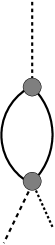
(a)

(b)

Figure 2. Spectrum obtained with the help of the regular Bohr-Sommerfeld rules. (a) Point of the Reeb graph, which correspond to the trajectories satisfying the quantization condition; (b) Semiclassical dispersion relations outside the separatrix region

2.2. Finite motion

Consider a spectral interval $\Delta=[E^{\prime},E^{\prime\prime}]$ such that for each $E\in\Delta$ the level set $H=E$ on the reduced phase space $\mathbb{T}^{2}_{px}$ consists of a single closed trajectory. In other word, the corresponding part of the Reeb graph must be an edge of finite motion; in the example shown in figure 1 the interval $[H_{+}+\delta,\max H]$, $\delta>0$, satisfies this condition; the corresponding edge is $e_{1}$. The regular Bohr-Sommerfeld rules select from the family of all these closed trajectories a discrete family of trajectories satisfying the quantization condition

$$\frac{1}{2\pi h}\oint p\,dx-\frac{1}{2}\in\mathbb{Z}.$$

(The construction of these trajectories can be interpreted as a selection of a certain discrete subset on all the edges of finite motion of the Reeb graph, see figure 2a). Each of these trajectories, $\Lambda$, implies a quasimode $(E,\psi)$, $E\in\mathbb{R}$, $\psi(x,h)\in L^{2}_{x}(\mathbb{R})$, with $\psi$ microlocally supported by $\Lambda$, $E=H|_{\Lambda}+O(h^{2})$, and $\big{\|}(\hat{H}_{h}-E)\psi\big{\|}/\|\psi\|=o(h^{\infty})$, which means that $\operatorname{dist}(\operatorname{spec}\hat{H}_{h},E)=o(h^{\infty})$. Clearly, to each of such $E$ there corresponds a whole family of quasimodes. Namely, if $\Lambda$ is a closed trajectory satisfying the quantization condition and $(E,\psi)$ is the corresponding quasimode, then the trajectory $\Lambda_{\mathbf{j}}:=\Lambda+(2\pi j_{1},2\pi j_{2})$, $\mathbf{j}=(j_{1},j_{2})\in\mathbb{Z}^{2}$, also satisfies the quantization condition and produces the quasimode $(E,\psi_{\mathbf{j}})$ with the same value $E$ and $\psi_{\mathbf{j}}(x,h)=\exp(2\pi ij_{1}x/h)\psi(x-2\pi j_{2},h)\equiv T_{1}^{-j_{1}}T_{2}^{-j_{2}}\psi(x,h)$. Let us try to satisfy the Bloch conditions by a function of the form

$$\Psi(x,\mathbf{k},h)=\sum_{\mathbf{j}=(j_{1},j_{2})\in\mathbb{Z}^{2}}C_{\mathbf{j}}(\mathbf{k},h)\psi_{\mathbf{j}}(x,h)=\sum_{\mathbf{j}=(j_{1},j_{2})\in\mathbb{Z}^{2}}C_{\mathbf{j}}(\mathbf{k},h)T_{1}^{-j_{1}}T_{2}^{-j_{2}}\psi(x,h).$$ (4)

Clearly, the coefficients $C_{\mathbf{j}}$ must solve a linear system: $C_{j_{1}+1,j_{2}}=C_{j_{1},j_{2}}e^{ik_{1}}$, $C_{j_{1},j_{2}+1}=C_{j_{1},j_{2}}e^{ik_{2}}$, $j_{1},j_{2}\in\mathbb{Z}$, therefore, $C_{\mathbf{j}}=ce^{i\langle\mathbf{j}|\mathbf{k}\rangle}$ for some constant $c$, and the corresponding Bloch quasimodes have the form

$$\Psi(x,\mathbf{k},h)=c\sum_{\mathbf{j}=(j_{1},j_{2})\in\mathbb{Z}^{2}}e^{i\langle\mathbf{j}|\mathbf{k}\rangle}e^{2\pi ij_{1}x/h}\psi(x-2\pi j_{2},h).$$ (5)

Therefore, to construct a Bloch quasimode in the form (4) we do not need to satisfy any additional conditions about relationship between $E$ and $\mathbf{k}$, which results in semiclassically constant dispersion relations.

If for each $E\in\Delta$ the level set $H$ contains several closed trajectories (and intersect several edges of finite motion (for example, it is the interval $[\min H,H_{-}-\delta]$ in the example of figure 1), the procedure described above is still applicable and gives the asymptotics of the spectrum up to $o(h^{\infty})$, but, in the case of some symmetries between families of trajectories degeneracies of the eigenvalues may occur; computation of their splitting is much more delicate [17, 5].

2.3. Infinite motion

Now consider the spectrum in the interval $\Delta=[E^{\prime},E^{\prime\prime}]$ assuming that the corresponding region of the Reeb graph consists of two edges of infinite motion (the interval $[H_{-}+\delta,H_{+}-\delta]$ and the edges $e_{2}$ and $e_{3}$ in the example of figure 1), i.e. for any $E\in\Delta$ the level set $H=E$ on $\mathbb{T}^{2}_{px}$ consists of two non-contractible trajectories, and in $\mathbb{R}^{2}_{px}$ there are two families of open periodic trajectories. Clearly, there exists a vector $\mathbf{d}=(d_{1},d_{2})\in\mathbb{Z}^{2}$, non-divisible by any other vector with integer-values components, such that for any of these trajectories, $\Lambda=\big{(}p=P(t),\ x=X(t)\big{)}$, there exists a nonzero number $T=T(\Lambda)$ satisfying $(P,X)(t+T)=(P,X)(t)+2\pi\mathbf{d}$ for all $t\in\mathbb{R}$. To simplify the calculation we assume that $\mathbf{d}=(1,0)$ (otherwise one can choose new canonical coordinates on the phase plane, such that $\mathbf{d}=(1,0)$ in these new coordinates). Obviously, there are two families of trajectories corresponding to different edges of the Reeb graph: for the first family, the number $T$ can be chosen positive, while for the another one it must be negative; we denote these families by $e^{+}$ and $e^{-}$ respectively.

Each trajectory $\Lambda^{\pm}=\big{(}p=P(t),x=X(t)\big{)}\in e^{\pm}$ implies a quasimode $(E^{\pm},\psi^{\pm})$, $E^{\pm}=H|_{\Lambda^{\pm}}+O(h^{2})$, satisfying $T_{2}\psi^{\pm}(x,h)\equiv\psi^{\pm}(x+2\pi,h)=\exp(iS^{\pm}(\Lambda^{\pm})/h)\psi^{\pm}(x,h)$, where

$$S^{\pm}(\Lambda^{\pm})=\int_{0}^{T}P^{\pm}(t)\,dX^{\pm}(t).$$ (6)

Clearly, the correspondence $E^{\pm}=H|_{\Lambda^{\pm}}\leftrightarrow\Lambda^{\pm}$ is one-to-one. Therefore, $S^{\pm}$ can be considered as a function of $E^{\pm}$, $S^{\pm}=S^{\pm}(E^{\pm})$. As this dependence is continuous and monotonic, it can be inverted: $E^{\pm}=E^{\pm}(S^{\pm})$; $E^{+}$ is an increasing function, while $E^{-}$ is a decreasing one.

Each $\Lambda^{\pm}$ implies a periodic family of trajectories $\Lambda^{\pm}_{j}:=\Lambda^{\pm}+(2\pi j,0)$ and corresponding quasimodes $(E^{\pm},\psi^{\pm}_{j})$ with $\psi^{\pm}_{j}(x,h)=\exp(2\pi ijx/h)\psi^{\pm}(x,h)\equiv T_{1}^{-j}\psi^{\pm}(x,h)$. To construct a Bloch quasimode we use an ansatz similar to that we use in the previous subsection,

$$\Psi^{\pm}(x,\mathbf{k},h)=\sum_{j\in\mathbb{Z}}C^{\pm}_{j}\psi^{\pm}_{j}(x,h)=\sum_{j\in\mathbb{Z}}C^{\pm}_{j}T_{1}^{-j}\psi^{\pm}(x,h).$$

Therefore, $C^{\pm}_{j+1}=C^{\pm}e^{2\pi ijk_{1}}$ ($C^{\pm}$ is a normalizing constant), and $S^{\pm}(E^{\pm})=h(n\mp k_{2}),\quad n\in\mathbb{Z}$. Denote $E^{\pm}_{n}(k_{2},h):=E^{\pm}\big{(}S^{\pm}=h(n\mp k_{2})\big{)}$; these functions can be viewed as semiclassical dispersion relations. Clearly, the functions $E^{+}_{n}$ are decreasing functions of $k_{2}$, while $E^{-}_{\pm}$ are increasing ones, therefore, in some critical points $k_{2}^{*}$ one has $E^{*}:=E^{-}_{n}(k_{2}^{*},h)=E^{+}_{m}(k_{2}^{*},h)$, as illustrated in figure 2b. The corresponding points $E^{*}$ are usually treated as approximations of gaps, more precisely, one expects that in $o(h^{\infty})$-neighborhood of each such value there is a gap, whose width is also $o(h^{\infty})$ [5]. The asymptotics of the true dispersion relations can be combined from pieces of $E^{+}_{n}$ and $E^{-}_{m}$ (figure 2b).

As we see, we have $o(h^{\infty})$-narrow bands in the first case and $o(h^{\infty})$-narrow gaps in the second case. Our aim is to describe the transition between two these two extremal cases, which correspond to the semiclassical asymptotics near separatrices. To obtain at least the first non-trivial term in the asymptotics of the width of $O(h^{\infty})$-small bands and gaps one should take into account the interaction between neighboring cells, which is an extremely different problem [17]. Such a calculation involves topological characteristics of the Hamiltonian, which results in a description of the quantized Hall conductance [13]. It is interesting to emphasize that the resulting topological numbers come from index-like characteristics of a certain path on the Reeb graph [5]; tjis provides an additional path index-like interpretation of the Chern classes, related to their their description through the cycle related to edges states on the Riemann surface of the Bloch functions [19].

3. Singular Bohr-Sommerfeld rules and their modification for the periodic problem

In this section, we give a short description of the semiclassical asymptotics near separatrices; this technique was developed in [14].

Let $H(p,x)$ be an arbitrary classical Hamiltonian (not necessary a Harper-like one) with non-degenerate critical points and $\hat{H}_{h}$ be the corresponding quantum Hamiltonian. Let $E$ be a critical value of $H$ in the sense that the level set $\Lambda:=\{(p,x)\in\mathbb{R}^{2}:H(p,x)=E\}$ contains a saddle point of $H$; our aim is to study the asymptotics of the spectrum of $\hat{H}_{h}$ in the interval $[E-Ah,E+Ah]$, $A>0$. We assume that $\Lambda$ is a compact connected set.

3.1. Preliminary constructions

Near the critical energy it is more convenient to use the scaled energy, i. e. we are going to solve the equation

$$(\hat{H}_{h}-E-\lambda h)\Psi=o(h^{\infty}),$$ (7)

where $\lambda$ is a new spectral value to be found; we consider the situation when $\lambda$ runs through some finite interval $[-A,A]$, $A>0$. The conditions which guarantee the existence of such solutions are called the singular Bohr-Sommerfeld rules.

Figure 3. Enumeration of edges near vertices

Due to the non-degeneracy of the saddle points, $\Lambda$ is a tetravalent graph embedded into the plane $\mathbb{R}^{2}_{px}$, and the saddle points are point of branching. The edges of the graph are smooth curves; each of these curves, $v$, delivers a part of solution by means of the usual WKB-asymptotics [18]; we denote this function by $\psi_{v}$. Our aim is to glue these contributions together near saddle points (vertices of the separatrix graph) in order to obtain a requested solution. Let us introduce a enumeration of the edges of the separatrix near each vertex in the following manner: the direct cyclic order is $v_{1},v_{4},v_{2},v_{3}$, and the quadrant formed by the edges $v_{1}$ and $v_{3}$ is pointed to the top, see figure 3. Near each vertex $\mathbf{V}$ we try to construct the requested solution in the form $\Psi=x_{1}^{\mathbf{V}}\psi_{v_{1}}\oplus x_{2}^{\mathbf{V}}\psi_{v_{2}}\oplus x_{3}^{\mathbf{V}}\psi_{v_{3}}\oplus x_{3}^{\mathbf{V}}\psi_{v_{3}}$, where $x_{j}^{\mathbf{V}}\in\mathbb{C}$, $j=1,2,3,4$. (Sometimes we omit the superscript $\mathbf{V}$ and write simply $x_{j}$.) Therefore, an edge can have different numbers near different vertices. To any vertex $\mathbf{V}$ of the graph we assign a so-called semiclassical invariant $\varepsilon^{\mathbf{V}}$ which is a formal power series in $h$,

$$\varepsilon^{\mathbf{V}}(\lambda,h)=\sum_{j=0}^{\infty}\varepsilon^{\mathbf{V}}_{j}(\lambda)h^{j},\quad\text{where}\quad\varepsilon^{\mathbf{V}}_{0}(\lambda)=\pm\frac{\lambda}{\sqrt{|\det H^{\prime\prime}(\mathbf{V})|}},\quad H^{\prime\prime}=\begin{pmatrix}H_{pp}&H_{px}\\ H_{xp}&H_{xx}\end{pmatrix}$$

and the sign $\pm$ coincides with the sign of $H$ in the quadrants formed by the edges 1 and 3.

Each cycle $\gamma$ on the graph $\Lambda$ will be accompanied by the following three characteristics (see [14] for details):

• Principal action $A_{\gamma}$,

  $$A_{\gamma}=\oint_{\gamma}p\ dx,$$

• Renormalized time $I_{\gamma}$. For cycles $\gamma$ crossing critical points with corners, we put

  $$I_{\gamma}=\operatorname{v.~{}p.}\oint_{\gamma}dt:=\sum_{j=1}^{n}\int_{\mathbf{c}_{j}}^{\mathbf{c}_{j+1}}dt,\quad\mathbf{c}_{j}\in\gamma,\quad\mathbf{c}_{1}=\mathbf{c}_{n+1},$$

  where the points $\mathbf{c}_{j}$ are chosen in such a way that each of the pieces $(\mathbf{c}_{j},\mathbf{c}_{j+1})\subset\gamma$ contains exactly one corner $\mathbf{V}_{j}$, and the integrals are calculated as

  $$\int_{\mathbf{c}_{j}}^{\mathbf{c}_{j+1}}dt:=\lim_{\mathbf{a},\mathbf{b}\to\mathbf{V}_{j}}\bigg{(}\int_{\mathbf{c}_{j}}^{\mathbf{a}}dt+\int_{\mathbf{b}}^{\mathbf{c}_{j+1}}dt+s_{j}\log\Big{|}\int_{R_{\mathbf{ab}}}dp\wedge dx\Big{|}\bigg{)},$$

  where $s_{j}:=\mp\lambda/\sqrt{|\det H^{\prime\prime}(\mathbf{V}_{j})|}$, and $R_{\mathbf{ab}}$ is a parallelogram spanned by the points $\mathbf{a}$, $\mathbf{V}_{j}$, and $\mathbf{b}$, and the sign $\mp$ is ”–” if the direction of integration corresponds to $dt$ and ”+” otherwise. By $dt$ we denote the Hamiltonian time, $dt(\operatorname{sgrad}H)=1$. This definition of $I_{\gamma}$ is then extended by additivity to all cycles (not necessary with corners).

• Maslov index $m_{\gamma}$. If none of the tangent to $\gamma$ at the corners is parallel to the $p$-axis, the index $m_{\gamma}$ is calculated as the sum of the indices of all the turning points in which $\gamma$ is smooth. If there are tangents parallel to the $p$-axis, one can destroy them by small variation; this must be reflected in the enumeration of edges near all the vertices.

3.2. Singular Bohr-Sommerfeld rules

The singular Bohr-Sommerfeld rules, which finally will result in conditions for $\lambda$, come from the following procedure.

Near each saddle point $\mathbf{V}$ there exist a canonical transformation $\chi(q,y)=(p,x)$, $\chi(\mathbf{O})=\mathbf{V}$, such that $H(p,x)=W(qy)qy$ with a certain smooth function $W$. This implies an elliptic Fourier integral operator $\hat{U}$ and a pseudodifferential operator $\hat{W}$, elliptic at the origin, such that $\hat{H}\hat{U}=\hat{U}\hat{W}(\widehat{yq}-h\varepsilon^{\mathbf{V}})$. Using this representation one can construct a microlocal basis $\psi_{j}$, $j=1,2,3,4$, of semiclassical solutions near $\mathbf{V}$. More precisely, we put

$$\varphi_{1}(y) =B^{\mathbf{V}}\frac{Y(y)}{\sqrt{|y|}}\ e^{i\varepsilon\log|y|}, \varphi_{2}(y) =B^{\mathbf{V}}\frac{Y(-y)}{\sqrt{|y|}}\ e^{i\varepsilon\log|y|},$$ (8)

$$\varphi_{3}(y) =B^{\mathbf{V}}\frac{e^{-i\pi/4}}{\sqrt{2\pi h}}\int_{\mathbb{R}}\frac{Y(t)}{\sqrt{|t|}}\ e^{iyt/h}\ e^{-\varepsilon\log|t|}dt, \varphi_{4}(y) =B^{\mathbf{V}}\frac{e^{-i\pi/4}}{\sqrt{2\pi h}}\int_{\mathbb{R}}\frac{Y(-t)}{\sqrt{|t|}}\ e^{iyt/h}\ e^{-\varepsilon\log|t|}dt,$$

where $Y$ is the Heaviside function, and then $\psi_{j}=\hat{U}\varphi_{j}$ is a basis element corresponding to the edge $j$, $j=1,2,3,4$. Here $B^{\mathbf{V}}$ is a normalizing constant.

A linear combination $x_{1}\psi_{1}\oplus x_{2}\psi_{2}\oplus x_{3}\psi_{3}\oplus x_{4}\psi_{4}$, $x_{j}\in\mathbb{C}$, $j=1,2,3,4$, which extends the WKB-solution to the saddle point, defines a function near $\mathbf{V}$ iff $x_{j}$’s satisfy the linear system

$$\begin{pmatrix}x_{3}\\ x_{4}\end{pmatrix}=\mathcal{E}\begin{pmatrix}1&ie^{-\varepsilon\pi}\\ ie^{-\varepsilon\pi}&1\end{pmatrix}\begin{pmatrix}x_{1}\\ x_{2}\end{pmatrix},\qquad\mathcal{E}:=\frac{1}{\sqrt{1+e^{-2\pi\varepsilon}}}e^{i\arg\Gamma(\frac{1}{2}+i\varepsilon)+i\varepsilon\log h},\qquad\varepsilon=\varepsilon^{\mathbf{V}}.$$ (9)

Clearly, $x_{j}$’s corresponding to different vertices must be connected with each other in a certain sense. To describe this correspondence we cut several edges in order to get a maximal tree on the separatrix. Now consider an arbitrary edge $v$ between two vertices $\mathbf{V}^{\prime}$ and $\mathbf{V}^{\prime\prime}$. Denote the corresponding $x$-coefficients by $x^{\prime}_{j}$ and $x^{\prime\prime}_{j}$ respectively, $j=1,2,3,4$, and assume that $v$ has index $j$ with respect to $\mathbf{V}^{\prime}$ and index $k$ with respect to $\mathbf{V}^{\prime\prime}$. We put

$$x^{\prime}_{j}=x^{\prime\prime}_{k},\quad\text{ if $v$ is not cut,}\qquad x^{\prime}_{j}=\operatorname{hol}\gamma\ x^{\prime\prime}_{k},\quad\text{ if $v$ is cut},$$ (10)

where $\operatorname{hol}\gamma$ is the so-called holonomy of the cycle $\gamma$ formed by the edge $e$ and the edges of the maximal tree (this cycle is unique). For the holonomy holds the estimate $|\operatorname{hol}\gamma|=1$, $\operatorname{Arg}\operatorname{hol}\gamma=A_{\gamma}/h+\lambda I_{\gamma}+\pi m_{\gamma}/2+O(h)$. Note that the first equality in (10) fix the constants $B^{\mathbf{V}}$ uniquely (up to a common multiplicator).

The equations (9) and (10) written for all the vertices and all the cycles respectively compose a linear system for the coefficients $x^{\mathbf{V}}_{j}$, $j=1,2,3,4$. The condition for the existence of non-trivial solutions (non-vanishing determinant) is called the singular Bohr-Sommerfeld rules.

3.3. Periodic problem

Our aim is to apply the singular Bohr-Sommerfeld rules to the Harper-like operators. The problem is that the level set of $E$ is always periodic and, respectively, unbounded. To apply this technique to the problem in question we take into account the Bloch conditions already at the stage of the construction of the solution (in contrast to the smooth case), in other words, we are going to apply the procedure described above for constructing the quasimode $\big{(}\Psi(x,\mathbf{k},h),E(\mathbf{k},h)\big{)}$ such that $\Psi$ satisfies (1) and (7). Clearly, this condition can be rewritten as the set of equalities $B^{\mathbf{V}+2\pi\mathbf{l}}=B^{\mathbf{V}}$, and $x_{j}^{\mathbf{V}+2\pi\mathbf{l}}=e^{i\langle\mathbf{l}|\mathbf{k}\rangle}x^{\mathbf{V}}_{j}$, $j=1,2,3,4$, for all vertices $\mathbf{V}$ and $\mathbf{l}\in\mathbb{Z}^{2}$, where $B^{\mathbf{V}}$ are constants from (8). This clarifies the meaning of the maximal tree in the periodic case: Instead of constructing a maximal tree in the whole plane it is sufficient to find a maximal tree on the reduced phase space $\mathbb{T}^{2}_{px}$; all the cycles will be viewed then as cycles on the torus.

4. Transition between finite and infinite motions

In this section, we consider spectral regions corresponding to the transition between closed and open trajectories. In this case the separatrices are non-compact in one direction only, and we assume that they are directed along the $x$-axis. Clearly, one can proceed first exactly in the same way as in the case of open trajectories, which will result in the following ansatz for the requested solution:

$$\Psi(x,\mathbf{k},h)=c\sum_{j\in\mathbb{Z}}e^{ijk_{1}}T_{1}^{-j}\psi(x,k_{2},h),$$

where $\psi$ must be a quasimode associated with the separatrix, $(\hat{H}_{h}-E-\lambda h)\psi=o(h^{\infty})$, and satisfying $T_{2}\psi=e^{ik_{2}}\psi$. It is clear that the corresponding semiclassical dispersion relations will not depend on $k_{1}$.

4.1. Two edges of infinite motion and one edge of finite motion

In this subsection, we consider probably the simplest structure of the separatrix. More precisely, we assume that the energy level $H=E$ on the reduced phase space $\mathbb{T}^{2}_{px}$ contains exactly one critical point, to be denoted by $\mathbf{V}$. The corresponding separatrix on the plane $\mathbb{R}^{2}_{px}$ has then the shape showed in figure 4. In terms of the Reeb graph this situation means that we consider a transition between two edges of infinite motions and one edge of finite motion. Near the corresponding branching point the Reeb graph has a $Y$-like shape. (We assume that the closed trajectories lie under the critical energy level.) Denote the semiclassical invariant of $\mathbf{V}$ by $\varepsilon(\lambda,h)$. Clearly,

$$\varepsilon(\lambda,h)=\lambda/w+O(h),\qquad w:=\sqrt{|\det H^{\prime\prime}(\mathbf{V})|}.$$ (11)

The separatrix on $\mathbb{T}^{2}_{px}$ is a graph with one vertex and two edges, $\gamma_{1}$ and $\gamma_{2}$, which are cycles on the torus, see figure 4. In order to obtain a maximal tree one has to cut both edges. Denote $\operatorname{hol}\gamma_{j}=:e^{i\alpha_{j}}$, $j=1,2$, where

$$\alpha_{j}=\frac{A_{j}}{h}+\lambda I_{j}+\frac{\pi m_{j}}{2}+O(h),\qquad A_{j}:=\oint_{\gamma_{j}}p\ dx,\quad I_{j}=\operatorname{v.~{}p.}\int_{\gamma_{j}}dt,\quad m_{j}=\operatorname{ind}\gamma_{j},\quad j=1,2.$$

To simplify the notation we put $x_{j}:=x^{\mathbf{V}}_{j}$, $y_{j}:=x^{\mathbf{V}+(0,2\pi)}_{j}$, $j=1,2,3,4$. The singular Bohr-Sommerfeld rules and the Bloch conditions lead us to the following equations:

$$\text{Bloch-periodicity conditions: }\quad y_{j}=e^{ik_{2}}x_{j},\quad j=1,2,3,4,$$

$$\text{Matching at $\mathbf{V}$: }\left\{\begin{aligned} x_{3}&=\mathcal{E}x_{1}+ie^{-\varepsilon\pi}\mathcal{E}x_{2}\\ x_{4}&=ie^{-\varepsilon\pi}\mathcal{E}x_{1}+\mathcal{E}x_{2},\end{aligned}\right.\qquad\text{Holonomy equations: }\left\{\begin{aligned} y_{3}&=e^{i\alpha_{1}}x_{1},&\text{ for }\gamma_{1},\\ x_{4}&=e^{i\alpha_{2}}y_{2},&\text{ for }\gamma_{2}.\end{aligned}\right.$$

where

$$\mathcal{E}:=\frac{1}{\sqrt{1+e^{-2\pi\varepsilon}}}e^{i\arg\Gamma(\frac{1}{2}+i\varepsilon)+i\varepsilon\log h},\\$$

The condition of existence of non-zero solutions is equivalent then to the equation

$$\cos\Big{(}\arg\Gamma\big{(}\frac{1}{2}+i\varepsilon\big{)}+\varepsilon\log h-\frac{\alpha_{1}+\alpha_{2}}{2}\Big{)}=\frac{1}{\sqrt{1+e^{-2\pi\varepsilon}}}\cos\Big{(}k_{2}-\frac{\alpha_{2}-\alpha_{1}}{2}\Big{)}.$$

The spectral parameter $\lambda$ enters this equation through $\varepsilon$, $\alpha_{1}$ and $\alpha_{2}$. One has obviously

$$\arg\Gamma\big{(}\frac{1}{2}+i\varepsilon\big{)}+\varepsilon\log h-\frac{\alpha_{1}+\alpha_{2}}{2}=\pm\arccos\frac{1}{\sqrt{1+e^{-2\pi\varepsilon}}}\,\cos\Big{(}k_{2}-\frac{\alpha_{2}-\alpha_{1}}{2}\Big{)}+2\pi n,\quad n\in\mathbb{Z}.$$

(a)

(b)

Figure 4. Transition between one edge of finite motion and two edges of infinite motion: (a) Structure of the separatrix, (b) The corresponding part of the Reeb graph

To find approximate solutions we represent $\lambda$ as $\lambda=\lambda_{0}+\mu$ with $\mu=o(1)$; in this way we can solve the equation near each $\lambda_{0}$. Taking into account Eq. (11) one can write

$$\arg\Gamma\Big{(}\frac{1}{2}+\frac{i\lambda_{0}}{w}\Big{)}+\frac{\lambda_{0}}{w}\log h+\frac{\mu}{w}\log h-\frac{(A_{1}+A_{2})}{2h}-\frac{I_{1}+I_{2}}{2}\lambda_{0}-\frac{\pi(m_{1}+m_{2})}{2}\\ {}=\pm\arccos\frac{1}{\sqrt{1+e^{-2\pi\lambda_{0}/w}}}\cos\Big{(}k_{2}-\frac{A_{2}-A_{1}}{2h}-\frac{I_{2}-I_{1}}{2}\lambda_{0}\Big{)}+2\pi n+O(\lambda)+O(h\log h),\quad n\in\mathbb{Z}$$

(one can show easily that $m_{1}-m_{2}=0$), or, finally,

$$\begin{gathered}\mu=\mu^{\pm}_{n}(k_{2},\lambda_{0},h)=\frac{w}{\log h}\,\bigg{\{}N(\lambda_{0},h)\pm\arccos\dfrac{\cos\big{(}k_{2}-\Delta(\lambda_{0},h)\big{)}}{\sqrt{1+e^{-2\pi\lambda_{0}/w}}}+2\pi n\bigg{\}}\,\bigg{[}1+O\Big{(}\frac{1}{\log h}\Big{)}\bigg{]}+O(h)\\ {}=\frac{w}{\log h}\times\bigg{\{}N(\lambda_{0},h)\pm\arccos\dfrac{\cos\Big{(}k_{2}-\Delta(\lambda_{0},h)\Big{)}}{\sqrt{1+e^{-2\pi\lambda_{0}/w}}}+2\pi n\bigg{\}}+o\Big{(}\frac{1}{\log h}\Big{)},\end{gathered}$$ (12)

where

$$N(\lambda_{0},h)=\frac{A_{1}+A_{2}}{2h}+\frac{\lambda_{0}(I_{1}+I_{2})+\pi(m_{1}+m_{2})}{2}-\frac{\lambda_{0}\log h}{w}-\arg\Gamma\Big{(}\frac{1}{2}+\frac{i\lambda_{0}}{w}\Big{)},$$

$$\Delta(\lambda_{0},h)=\dfrac{A_{2}-A_{1}}{2h}+\lambda_{0}\dfrac{I_{2}-I_{1}}{2}$$

and $n$ are integers such that the expression in the curly brackets in (12) is $o(\log h)$. Returning to the original spectral parameter we obtain a series of semiclassical dispersion relations: in a $o(h)$-neighborhood of $E+\lambda_{0}h$ they take the form $E^{\pm}_{n}(k_{1},k_{2},\lambda_{0},h)=E+\lambda_{0}h+h\mu^{\pm}_{n}(k_{2},\lambda_{0},h)$. The expression obtained can be used for estimating the band- and the gapwidth. More precisely, the bands and the gaps in a $o(h)$-neighborhood of $E+\lambda_{0}h$ have the width

$$B(\lambda_{0},h)=\frac{2wh}{|\log h|}\arcsin\frac{1}{\sqrt{1+e^{-2\pi\lambda_{0}/w}}}+o\Big{(}\frac{h}{\log h}\Big{)},$$ (13)

$$G(\lambda_{0},h)=\frac{2wh}{|\log h|}\arccos\frac{1}{\sqrt{1+e^{-2\pi\lambda_{0}/w}}}+o\Big{(}\frac{h}{\log h}\Big{)}$$ (14)

respectively. In particular, for $\lambda_{0}=0$ the bands and the gaps have approximately the same width $\pi wh/(2|\log h|)$.

4.2. Two edges of infinite motion and two edges of finite motion

We consider now another structure of the separatrix. Let us assume that the energy level $H=E$ on the reduced phase space is a connected set containing two critical points, which we denote by $\mathbf{V}$ and $\tilde{\mathbf{V}}$. The separatrix has the shape sketched in figure 5. The Reeb graph has near the corresponding branching point a $X$-like shape, where the two upper edges correspond to open trajectories.

(a)

(b)

Figure 5. Transition between two edges of finite motion and two edges of infinite motion: (a) Structure of the separatrix, (b) The corresponding part of the Reeb graph.

Denote the semiclassical invariants of $\mathbf{V}$ and $\tilde{\mathbf{V}}$ by $\varepsilon$ and $\tilde{\varepsilon}$ respectively,

$$\varepsilon(\lambda,h)=\lambda/w+O(h),\quad\tilde{\varepsilon}=\lambda/\tilde{w}+O(h),\qquad w:=\sqrt{\big{|}\det H^{\prime\prime}(\mathbf{V})\big{|}},\quad\tilde{w}:=\sqrt{\big{|}\det H^{\prime\prime}(\tilde{\mathbf{V}})\big{|}},$$ (15)

and put

$$\mathcal{E}:=\frac{\exp\left[i\arg\Gamma\Big{(}\frac{1}{2}+i\varepsilon\Big{)}+i\varepsilon\log h,\right]}{\sqrt{\displaystyle 1+e^{-2\pi\varepsilon}}},\qquad\tilde{\mathcal{E}}:=\frac{\exp\left[i\arg\Gamma\Big{(}\frac{1}{2}+i\tilde{\varepsilon}\Big{)}+i\tilde{\varepsilon}\log h,\right]}{\sqrt{\displaystyle 1+e^{-2\pi\tilde{\varepsilon}}}}$$ (16)

In order to obtain a maximal tree on the reduced phase space we cut all the edges but $\gamma_{1}$, then one get three cycles: $\tilde{\gamma}_{1}=\gamma_{1}+\gamma_{2}$, $\tilde{\gamma}_{2}=\gamma_{4}-\gamma_{1}$, and $\tilde{\gamma}_{3}=\gamma_{1}+\gamma_{3}$; put $\alpha_{j}:=\arg\operatorname{hol}\tilde{\gamma}_{j}$, $j=1,2,3$.

Denote $x_{j}:=x^{\mathbf{V}}_{j}$, $y_{j}:=x^{\tilde{\mathbf{V}}}_{j}$, $z_{j}:=x^{\mathbf{V}+(0,2\pi)}_{j}$, $j=1,2,3,4$, then the quantization conditions are:

$$\text{Bloch-periodicity conditions:}\quad z_{j}=e^{ik_{2}}x_{j},\quad j=1,2,3,4,$$

$$\text{Matching conditions at $\mathbf{V}$: }\left\{\begin{aligned} x_{3}&=\mathcal{E}x_{1}+ie^{-\varepsilon\pi}\mathcal{E}x_{2},\\ x_{4}&=ie^{-\varepsilon\pi}\mathcal{E}x_{1}+\mathcal{E}x_{2},\end{aligned}\right.\quad\text{at $\tilde{\mathbf{V}}$: }\left\{\begin{aligned} y_{3}&=\tilde{\mathcal{E}}y_{1}+ie^{-\tilde{\varepsilon}\pi}\tilde{\mathcal{E}}y_{2},\\ y_{4}&=ie^{-\tilde{\varepsilon}\pi}\tilde{\mathcal{E}}y_{1}+\tilde{\mathcal{E}}y_{2},\end{aligned}\right.$$

$$\text{Holonomy equations: }y_{2}=x_{4},\quad y_{3}=e^{i\alpha_{1}}x_{1},\quad z_{3}=e^{i\alpha_{2}}y_{1},\quad y_{4}=e^{i\alpha_{3}}z_{2}.$$

The condition of the existence of non-trivial solutions leads to the equation

$$\cos\bigg{(}\arg\Gamma\Big{(}\frac{1}{2}+i\varepsilon\Big{)}+\arg\Gamma\Big{(}\frac{1}{2}+i\tilde{\varepsilon}\Big{)}+(\varepsilon+\tilde{\varepsilon})\log h-\frac{\alpha_{1}+\alpha_{2}+\alpha_{3}}{2}\bigg{)}\\ {}=\dfrac{1}{\displaystyle\sqrt{(1+e^{-\varepsilon\pi})(1+e^{-\tilde{\varepsilon}\pi})}}\bigg{(}\cos\Big{(}k_{2}-\frac{\alpha_{1}+\alpha_{2}-\alpha_{3}}{2}\Big{)}-e^{-(\varepsilon+\tilde{\varepsilon})\pi}\cos\frac{\alpha_{1}-\alpha_{2}-\alpha_{3}}{2}\bigg{)}.$$ (17)

The parameter $\lambda$ enters this equation through $\varepsilon$, $\tilde{\varepsilon}$, and $\alpha_{j}$, $j=1,2,3$.

To obtain a more clear picture, let us introduce holonomies of the edges as solutions of the following equalities: $\alpha_{1}=\beta_{1}+\beta_{2}$, $\alpha_{2}=\beta_{4}-\beta_{1}$, $\alpha_{3}=\beta_{1}+\beta_{3}$, $\arg\operatorname{hol}(\tilde{\gamma}_{2}+\tilde{\gamma}_{4})=\beta_{2}+\beta_{4}$; these solutions can be represented as

$$\beta_{j}=\frac{B_{j}}{h}+\lambda J_{j}+\frac{\pi m_{j}}{2}+O(h),\quad B_{j}=\int_{\gamma_{j}}p\ dx,\quad m_{j}=\operatorname{ind}\gamma_{j},\quad j=1,2,3,4,$$

then (17) takes the form

$$\arg\Gamma\Big{(}\frac{1}{2}+i\varepsilon\Big{)}+\arg\Gamma\Big{(}\frac{1}{2}+i\tilde{\varepsilon}\Big{)}+(\varepsilon+\tilde{\varepsilon})\log h-\frac{\beta_{1}+\beta_{2}+\beta_{3}+\beta_{4}}{2}\\ {}\quad=\pm\arccos\dfrac{\cos\Big{(}k_{2}-\frac{(\beta_{2}+\beta_{4})-(\beta_{1}+\beta_{3})}{2}\Big{)}-e^{-(\varepsilon+\tilde{\varepsilon})\pi}\cos\frac{(\beta_{1}+\beta_{2})-(\beta_{3}+\beta_{4})}{2}}{\displaystyle\sqrt{(1+e^{-\varepsilon\pi})(1+e^{-\tilde{\varepsilon}\pi})}}+2\pi n,\quad n\in\mathbb{Z}.$$ (18)

The quantities $\beta_{j}$ can be viewed as “weights” of the separatrice edges, then Eq. (18) shows how the relationship between them influences the dispersion relations.

Like in the previous case we represent $\lambda$ as $\lambda_{0}+\mu$, $\mu=o(1)$, and solve (approximately) the equation for $\mu$. The solutions take the form

$$\begin{gathered}\mu=\mu_{n}^{\pm}(k_{2},\lambda_{0},h)=\frac{w\tilde{w}}{(w+\tilde{w})\log h}\times\bigg{\{}N(\lambda_{0},h)\\ {}\pm\arccos\frac{\cos\big{(}k_{2}-\Delta_{2}(\lambda_{0},h)\big{)}-e^{-(1/w+1/\tilde{w})\lambda_{0}\pi}\cos\Delta_{1}(\lambda_{0},h)}{\sqrt{(1+e^{-2\pi\lambda_{0}/w})(1+e^{-2\pi\lambda_{0}/\tilde{w}})}}+2\pi n\bigg{\}}\times\bigg{(}1+O\Big{(}\frac{1}{\log h}\Big{)}\bigg{)}+O(h),\end{gathered}$$ (19)

where

$$N(\lambda_{0},h) :=\frac{B_{1}+B_{2}+B_{3}+B_{4}}{2h}+\lambda_{0}\frac{J_{1}+J_{2}+J_{3}+J_{4}}{2}+\frac{\pi(m_{1}+m_{2}+m_{3}+m_{4})}{2}$$

$$\qquad{}-\arg\Gamma\Big{(}\frac{1}{2}+\frac{i\lambda_{0}}{w}\Big{)}-\arg\Gamma\Big{(}\frac{1}{2}+\frac{i\lambda_{0}}{\tilde{w}}\Big{)}-\lambda_{0}\Big{(}\frac{1}{w}+\frac{1}{\tilde{w}}\big{)}\log h,$$

$$\Delta_{1}(\lambda_{0},h) :=\dfrac{(B_{1}+B_{2})-(B_{3}+B_{4})}{2h}+\lambda_{0}\dfrac{(J_{1}+J_{2})-(J_{3}+J_{4})}{2},$$

$$\Delta_{2}(\lambda_{0},h) :=\frac{(B_{2}+B_{4})-(B_{1}+B_{3})}{2h}+\lambda_{0}\frac{(J_{2}+J_{4})-(J_{1}+J_{3})}{2}$$

and $n\in\mathbb{Z}$, $n=[N(\lambda_{0},h)]+o(\log h)$. The dispersion relations are $E(k_{1},k_{2},h)=E+h\lambda_{0}+h\mu^{\pm}_{n}(k_{2},\lambda_{0},h)$. In contrast to the previous situation, band and gaps have, generally speaking, different width. More precisely, near the point $E+\lambda_{0}h$ one has bands having the width

$$B(\lambda_{0},h)=\frac{w\tilde{w}h}{(w+\tilde{w})|\log h|}\bigg{[}\arcsin\frac{1+e^{-(1/w+1/\tilde{w})\lambda_{0}\pi}\cos\ \Delta_{1}(\lambda_{0},h)}{\sqrt{(1+e^{-2\pi\lambda_{0}/w})(1+e^{-2\pi\lambda_{0}/\tilde{w}})}}\\ {}+\arcsin\frac{1-e^{-(1/w+1/\tilde{w})\lambda_{0}\pi}\cos\ \Delta_{1}(\lambda_{0},h)}{\sqrt{(1+e^{-2\pi\lambda_{0}/w})(1+e^{-2\pi\lambda_{0}/\tilde{w}})}}\bigg{]}+o\Big{(}\frac{h}{\log h}\Big{)},$$ (20)

and two groups of gaps having the width

$$G_{1}(\lambda_{0},h)=\frac{2w\tilde{w}h}{(w+\tilde{w})|\log h|}\arccos\frac{1+e^{-(1/w+1/\tilde{w})\lambda_{0}\pi}\cos\ \Delta_{1}(\lambda_{0},h)}{\sqrt{(1+e^{-2\pi\lambda_{0}/w})(1+e^{-2\pi\lambda_{0}/\tilde{w}})}}+o\Big{(}\frac{h}{\log h}\Big{)},$$ (21)

$$G_{2}(\lambda_{0},h)=\frac{2w\tilde{w}h}{(w+\tilde{w})|\log h|}\arccos\frac{1-e^{-(1/w+1/\tilde{w})\lambda_{0}\pi}\cos\ \Delta_{1}(\lambda_{0},h)}{\sqrt{(1+e^{-2\pi\lambda_{0}/w})(1+e^{-2\pi\lambda_{0}/\tilde{w}})}}+o\Big{(}\frac{h}{\log h}\Big{)},$$ (22)

and they come in groups $\dots,B,G_{1},B,G_{2},\dots$, The formulas clearly show the fast decaying of the bandwidth for negative $\lambda_{0}$ and of the gapwidth for positive $\lambda_{0}$. From the other side, the ratio bandwidth/gapwidth depends crucially on the relationship between $B_{j}$, $J_{j}$, $\lambda_{0}$, and $h$.

5. Transition between topologically different finite motions (degenerate case)

(a)

(b)

Figure 6. Transition between two edges of finite motion: (a) Structure of the separatrix, (b) The corresponding part of the Reeb graph.

In this section we consider a situation when all the smooth trajectories of the classical Hamiltonian are closed. This situation takes place if, for example, $H$ is invariant under linear transformation having no real eigenvectors (rotation by $\pi/2$, for example). More precisely, we assume that the level set $H=E$ on the reduced space contains two critical points, which we denote by $\mathbf{V}$ and $\tilde{\mathbf{V}}$, and the corresponding separatrix in the plane is non-compact in all directions. This situation is illustrated in figure 6. We can expect that the semiclassical dispersion relations in this case depend on both quasimomenta $k_{1}$ and $k_{2}$. Denote by $\varepsilon$ and $\tilde{\varepsilon}$ the semiclassical invariants of $\mathbf{V}$ and $\tilde{\mathbf{V}}$ respectively, and use the notation of (16). Clearly,

$$\varepsilon=\lambda/w+O(h),\quad\tilde{\varepsilon}=-\lambda/\tilde{w}+O(h),\qquad w=\sqrt{\big{|}\det H^{\prime\prime}(\mathbf{V})\big{|}},\quad\tilde{w}=\sqrt{\big{|}\det H^{\prime\prime}(\tilde{\mathbf{V}})\big{|}}.$$

An essential point is that the main terms of $\varepsilon$ and $\tilde{\varepsilon}$ have opposite signs.

We fix a maximal tree by cutting all the edges but $\gamma_{1}$, then three cycles appear: $\tilde{\gamma}_{1}=\gamma_{4}+\gamma_{1}$, $\tilde{\gamma}_{2}=\gamma_{3}-\gamma_{1}$, and $\tilde{\gamma}_{2}=\gamma_{2}+\gamma_{1}$ with holonomies $e^{i\alpha_{j}}$, $j=1,2,3$, respectively. Put $x_{j}:=x^{\mathbf{V}}_{j}$, $y_{j}:=x^{\tilde{\mathbf{V}}}_{j}$, $z_{j}:=x^{\mathbf{V}+(0,2\pi)}_{j}$, $w_{j}:=x^{\tilde{\mathbf{V}}+(2\pi,0)}_{j}$, $j=1,2,3,4$, then we come to the following set of equalities:

$$\text{Bloch-periodicity conditions: }w_{j}=e^{ik_{1}}y_{j},\quad z_{j}=e^{ik_{2}}x_{j},\quad j=1,2,3,4,$$

$$\text{Matching conditions at $\mathbf{V}$:}\left\{\begin{aligned} x_{3}&=\mathcal{E}x_{1}+ie^{-\varepsilon\pi}\mathcal{E}x_{2},\\ x_{4}&=ie^{-\varepsilon\pi}\mathcal{E}x_{1}+\mathcal{E}x_{2},\end{aligned}\right.\quad\text{at $\tilde{\mathbf{V}}$: }\left\{\begin{aligned} y_{3}&=\tilde{\mathcal{E}}y_{1}+ie^{-\tilde{\varepsilon}\pi}\tilde{\mathcal{E}}y_{2},\\ y_{4}&=ie^{-\tilde{\varepsilon}\pi}\tilde{\mathcal{E}}y_{1}+\tilde{\mathcal{E}}y_{2},\end{aligned}\right.$$

$$\text{Holonomy equations: }x_{4}=y_{3},\quad w_{2}=e^{i\alpha_{1}}x_{1},\quad z_{3}=e^{i\alpha_{2}}w_{4},\quad y_{1}=e^{i\alpha_{3}}z_{2}.$$

After some algebra one arrives at a $2\times 2$ linear system,

$$\begin{pmatrix}\mathcal{E}-\tilde{\mathcal{E}}e^{i(\alpha_{1}+\alpha_{2}-k_{2})}&ie^{-\varepsilon\pi}\mathcal{E}-ie^{-\tilde{\varepsilon}\pi}\tilde{\mathcal{E}}e^{i(k_{1}+\alpha_{2}+\alpha_{3})}\phantom{\bigg{|}}\\ ie^{-\varepsilon\pi}\mathcal{E}-ie^{-\tilde{\varepsilon}\pi}\tilde{\mathcal{E}}e^{i(\alpha_{1}-k_{1})}&\mathcal{E}-\tilde{\mathcal{E}}e^{i(k_{2}+\alpha_{3})}\end{pmatrix}\begin{pmatrix}x_{1}\\ x_{2}\end{pmatrix}=0.$$

The condition for the last system to have non-trivial solutions comes from the vanishing of its determinant and has the form

$$\cos\bigg{[}\arg\Gamma\Big{(}\frac{1}{2}+i\varepsilon\Big{)}-\arg\Gamma\Big{(}\frac{1}{2}+i\tilde{\varepsilon}\Big{)}+(\varepsilon-\tilde{\varepsilon})\log h-\frac{\alpha_{1}+\alpha_{2}+\alpha_{3}}{2}\bigg{]}\\ =\frac{1}{\sqrt{\big{(}1+e^{-2\varepsilon\pi}\big{)}\big{(}1+e^{-2\tilde{\varepsilon}\pi}\big{)}}}\bigg{[}e^{-(\varepsilon+\tilde{\varepsilon})\pi}\cos\Big{(}k_{1}-\frac{\alpha_{1}-\alpha_{2}-\alpha_{3}}{2}\Big{)}+\cos\Big{(}k_{2}-\frac{\alpha_{1}+\alpha_{2}-\alpha_{3}}{2}\Big{)}\bigg{]}.$$ (23)

Introducing again the weights $\beta_{j}$ of the edges $\gamma_{j}$, $j=1,2,3,4$, by the rule

$$\alpha_{1}=\beta_{4}+\beta_{1},\quad\alpha_{2}=\beta_{3}-\beta_{1},\quad\alpha_{3}=\beta_{2}-\beta_{1},\quad\arg\operatorname{hol}(\gamma_{2}+\gamma_{3})=\beta_{2}+\beta_{3},$$

$$\beta_{j}=\frac{B_{j}}{h}+\lambda J_{j}+\frac{\pi m_{j}}{2}+O(h),\quad B_{j}=\int_{\gamma_{j}}p\ dx,\quad m_{j}=\operatorname{ind}\gamma_{j},\quad j=1,2,3,4.$$

we rewrite (23) as

$$\cos\bigg{[}\arg\Gamma\Big{(}\frac{1}{2}+i\varepsilon\Big{)}-\arg\Gamma\Big{(}\frac{1}{2}+i\tilde{\varepsilon}\Big{)}+(\varepsilon-\tilde{\varepsilon})\log h-\frac{\beta_{1}+\beta_{2}+\beta_{3}+\beta_{4}}{2}\bigg{]}\\ =\frac{e^{-(\varepsilon+\tilde{\varepsilon})\pi}\cos\Big{(}k_{1}-\frac{(\beta_{1}+\beta_{4})-(\beta_{2}+\beta_{3})}{2}\Big{)}+\cos\Big{(}k_{2}-\frac{(\beta_{3}+\beta_{4})-(\beta_{1}+\beta_{2})}{2}\Big{)}}{\sqrt{\big{(}1+e^{-2\varepsilon\pi}\big{)}\big{(}1+e^{-2\tilde{\varepsilon}\pi}\big{)}}}.$$ (24)

Representing again $\lambda=\lambda_{0}+\mu$, $\mu=o(1)$, we come to the following expression for $\mu$:

$$\begin{gathered}\mu=\mu^{\pm}_{n}(k_{1},k_{2},\lambda_{0},h)=\frac{w\tilde{w}}{(w+\tilde{w})\log h}\\ {\times}\bigg{\{}N(\lambda_{0},h)\pm\arccos\frac{e^{-\pi\lambda_{0}/w}\cos\big{(}k_{1}-\Delta_{1}(\lambda_{0},h)\big{)}+e^{-\pi\lambda_{0}/\tilde{w}}\cos\big{(}k_{2}-\Delta_{2}(\lambda_{0},h)\big{)}}{\sqrt{(1+e^{-2\pi\lambda_{0}/w})(1+e^{-2\pi\lambda_{0}/\tilde{w}})}}+2\pi n\bigg{\}}\\ {}\times\Big{(}1+O\big{(}\frac{1}{\log h}\big{)}\Big{)}+O(h),\end{gathered}$$ (25)

where

$$N(\lambda_{0},h) =\frac{B_{1}+B_{2}+B_{3}+B_{4}}{2h}+\frac{J_{1}+J_{2}+J_{3}+J_{4}}{2}\ \lambda_{0}+\frac{\pi(m_{1}+m_{2}+m_{3}+m_{4})}{2}$$

$$\quad{}-(\frac{1}{w}+\frac{1}{\tilde{w}})\lambda_{0}\log h-\arg\Gamma\Big{(}\frac{1}{2}+\frac{i\lambda_{0}}{w}\Big{)}+\arg\Gamma\Big{(}\frac{1}{2}-\frac{i\lambda_{0}}{\tilde{w}}\Big{)},$$

$$\Delta_{1}(\lambda_{0},h) =\frac{(B_{1}+B_{4})-(B_{2}+B_{3})}{2h}+\lambda_{0}\frac{(J_{1}+J_{4})-(J_{2}+J_{3})}{2},$$

$$\Delta_{2}(\lambda_{0},h) =\frac{(B_{3}+B_{4})-(B_{1}+B_{2})}{2h}+\lambda_{0}\frac{(J_{3}+J_{4})-(J_{1}+J_{2})}{2}.$$

The bandswidth $B(\lambda_{0},h)$ and the gapwidth $G(\lambda_{0},h)$ in a $o(h)$-neighborhood of the point $E+\lambda_{0}h$ admit a simple estimate

$$B(\lambda_{0},h)=\frac{2w\tilde{w}h}{(w+\tilde{w})|\log h|}\arcsin\frac{e^{-\pi\lambda_{0}/w}+e^{-\pi\lambda_{0}/\tilde{w}}}{\sqrt{(1+e^{-2\pi\lambda_{0}/w})(1+e^{-2\pi\lambda_{0}/\tilde{w}})}}+o\Big{(}\frac{h}{\log h}\Big{)},$$ (26)

$$G(\lambda_{0},h)=\frac{2w\tilde{w}h}{(w+\tilde{w})|\log h|}\arccos\frac{e^{-\pi\lambda_{0}/w}+e^{-\pi\lambda_{0}/\tilde{w}}}{\sqrt{(1+e^{-2\pi\lambda_{0}/w})(1+e^{-2\pi\lambda_{0}/\tilde{w}})}}+o\Big{(}\frac{h}{\log h}\Big{)},$$ (27)

so that the bands clearly show an exponential decay with respect to $|\lambda_{0}|$.

6. Discussion

In this section, we discuss in greater detail the influence of characteristics of the Hamiltonian $H$ on the dispersion relation.

In the case of subsection 4.1 the picture is quite simple. The semiclassical dispersion relations depend on one of the quasimomenta only, and the extremum points (with respect to this quasimomentum $k_{2}$) is determined by the difference between the upper and the lower part of the separatrix, $\gamma_{1}$ and $\gamma_{2}$; the width of the bands and the gaps, which is given by Eqs. (13) and  (14) respectively, depends on the determinant of the second derivatives at the critical point; these formulas present a generalization of a similar estimate for the periodic Sturm-Liouville problem (see, for example, [14, Sec. 10]).

The example considered in subsection 4.2 and figure 5 differs from the previous one. The position of the extremum point with respect to $k_{2}$ is, like in the previous case, determined by the relationship between the upper $\gamma_{2}+\gamma_{4}$ and the lower $\gamma_{1}+\gamma_{3}$ parts of the separatrix. But the band- and the gapwidths, as can be seen from (20), (21), and (22), crucially depend on $\Delta_{1}$; the quantity $\Delta_{1}$ can be interpreted as a “difference” between the cycles $\gamma_{1}+\gamma_{2}$ and $\gamma_{3}+\gamma_{4}$. For example, if the areas of these two cycles do not coincide, the ratio bandwidth/gapwidth has no limit for $h\to 0$. Examples with more complicated separatrices will show a more curious picture.

$\lambda_{0}>0$

$\lambda_{0}=0$

$\lambda_{0}<0$

Figure 7. Levels curves of the dispersion relations lying near $E+\lambda_{0}h$

The example of section 5 shows a regular behavior of the band and the gaps; the main term in the asymptotic of their width, Eqs. (26) and (27), like in the first example, is determined by the second derivatives at the critical points only. From the other side, this example is suitable for discussing the form of the energy bands. The dispersion relations lying in a neighborhood of $E+\lambda_{0}h$ have maxima at the points

$$\mathbf{k}=\mathbf{k}_{\mathrm{max}}(\lambda_{0},h):=\bigg{(}2\pi\times\Big{\{}\frac{\Delta_{1}(\lambda_{0},h)}{2\pi}+\frac{1}{2}\Big{\}}-\pi,2\pi\times\Big{\{}\frac{\Delta_{2}(\lambda_{0},h)}{2\pi}+\frac{1}{2}\Big{\}}-\pi\bigg{)}$$ (28)

(here $\{x\}$ denotes the fractional part of $x$). In the generic situation, when all the holonomies $\beta_{j}$ are different, these points depend crucially on $\lambda_{0}$, $B_{j}$, $I_{j}$, and $h$, so that a small variation of them can change $\mathbf{k}_{\mathrm{max}}$ significantly. Near the critical energy $E$ (i.e. for $\lambda_{0}=0$), the quasimomenta have “equal rights”, i. e. the coefficients before $\cos$-terms in (25) are approximately equal to $1$. In the non-symmetric case, when $w\neq\tilde{w}$, the situation changes for non-zero $\lambda_{0}$. So, if $w>\tilde{w}$, the quasimomentum $k_{1}$ dominates if $\lambda_{0}>0$ and $k_{2}$ dominates for $\lambda_{0}<0$, and, at the same time the maxima of the dispersion relations moves according to (28), see illustration in figure 7. This gives a rather rough (but at the same time generic) impression about the dispersion relation structure near the critical point.

Appendix. The periodic Landau Hamiltonian with a strong magnetic field and Harper-like operators

In this appendix, we briefly describe the relationship between the periodic Landau operator and Harper-like operators as it was established and studied in [4, 11, 20].

The periodic Landau Hamiltonian has the form

$$\hat{L}:=\frac{1}{2}\Big{(}-ih\frac{\partial}{\partial x_{1}}+x_{2}\Big{)}^{2}-\frac{h^{2}}{2}\frac{\partial^{2}}{\partial x_{2}}+\varepsilon v(x_{1},x_{2}),$$

where $v$ is a two-periodic function with periods $\mathbf{a}$ and $\mathbf{b}$. If $\varepsilon=0$, the spectrum of $\hat{L}$ consists of infinitely degenerate eigenvalues $I_{n}=(n+1/2)h$, $n\in\mathbb{Z}_{+}$, called Landau levels. The presence of non-zero $\varepsilon$ leads to a broadening of these numbers into a certain sets called Landau bands. We are going to show, under assumption that both $h$ and $\varepsilon$ are small, that the broadening of each Landau level is described by a certain Harper-like operator.

The corresponding to $\hat{L}$ classical Hamiltonian is $L(p,x,\varepsilon)=(p_{1}+x_{2})^{2}/2+p_{2}^{2}/2+\varepsilon v(x_{1},x_{2})$. If $\varepsilon=0$, then $L$ defines an integrable system whose trajectories on the $(x_{1},x_{2})$-plane are cyclotron orbits. For non-zero $\varepsilon$ the Hamiltonian is non-integrable, but, for small $\varepsilon$, one can interpret the classical dynamics as a cyclotron motion around a guiding center. We introduce new canonical coordinates connected the motion of the center: $p_{1}=-y_{2}$, $p_{2}=-q$, $x_{1}=q+y_{1}$, $x_{2}=p+y_{2}$, considering $(p,y_{1})$ as generalized momenta and $(q,y_{2})$ as generalized positions ($p,q$ describe the motion around the center with the coordinates $y_{1},y_{2}$), then $H$ takes the form $L=(p^{2}+q^{2})/2+\varepsilon v(q+y_{1},p+y_{2})$. Introduce the averaged Hamiltonian

$$\bar{L}(I,y_{1},y_{2},\varepsilon)=I+\frac{1}{2\pi}\oint v(\sqrt{2I}\sin\varphi+y_{1},\sqrt{2I}\cos\varphi+y_{2})\,d\varphi\equiv I+J_{0}(\sqrt{-2I\Delta_{y}})v(y_{1},y_{2}),$$

where $J_{0}$ is the Bessel function of order zero and $\Delta_{y}=\partial^{2}/\partial y_{1}^{2}+\partial^{2}/\partial y_{2}^{2}$. One can show that there exists a canonical change of variables $(p,y_{1},q,y_{2})=(\bar{p},\bar{y}_{1},\bar{q},\bar{y}_{2})+O(\varepsilon)$, periodic in $y_{1},y_{2}$ with periods $\mathbf{a}$ and $\mathbf{b}$, such that $L=\bar{L}\big{(}({\bar{p}}^{2}+{\bar{q}}^{2})/2,\bar{y}_{1},\bar{y}_{2},\varepsilon\big{)}+O(\varepsilon^{2})$. The averaging procedure can be iterated, so that one constructs an averaged Hamiltonian $\mathcal{L}=\mathcal{L}(J,Y_{1},Y_{2},\varepsilon)$ and a canonical change of variables $(p,y_{1},q,y_{2})=(P,Y_{1},Q,Y_{2})+O(\varepsilon)$, both periodic in $y_{1},y_{2}$, such that $L=\mathcal{L}\big{(}(P^{2}+Q^{2})/2,Y_{1},Y_{2},\varepsilon\big{)}+O(\varepsilon^{\infty})$. Therefore, neglecting the last term and using the canonicity of all the transformations one reduces the spectral problem for $\hat{L}$ to that for $\hat{\mathcal{L}}$ obtained from $\mathcal{L}$ by the Weyl quantization ($P=-ih\partial/\partial Q$, $Y_{1}=-ih\partial/\partial Y_{2}$):

$$\hat{\mathcal{L}}\Psi(Q,Y_{2})=E\Psi(Q,Y_{2}).$$ (29)

Clearly, $\hat{\mathcal{L}}$ commutes with the harmonic oscillator $\hat{I}:=(-h^{2}\partial^{2}/\partial Q^{2}+Q^{2})/2$, which means that the eigenfunction $\Psi$ in (29) can be represented as $\Psi(Q,Y_{2})=\psi_{n}(Q)\Phi(Y_{2})$, where $\psi_{n}$ is an eigenfunction of $\hat{I}$ with the eigenvalue $I_{n}$, and $\Phi$ must be an eigenfunction of the operator $\hat{L}_{n}$ obtained by quantizing the classical Hamiltonian $L_{n}(Y_{1},Y_{2})=\mathcal{L}(I_{n},Y_{1},Y_{2},\varepsilon)$ considering $Y_{1}$ as a momentum and $Y_{2}$ as a position. All these Hamiltonians $L_{n}$ are periodic in $Y_{1}$ and $Y_{2}$, therefore, after a linear symplectic transformation $\hat{L}_{n}$ becomes a certain Harper-like operator which can be treated as a Hamiltonian describing the broadening of Landau level under the presence of the electric potential $v$.

(a)

(b)

(c)

Figure 8. Level curves in the elementary cell $[0,2\pi)\times[0,\pi)$: (a) of the potential $v$, (b) of the averaged Hamiltonian for $I\approx 0.5$, (c) of the averaged Hamiltonian for $I\approx 1.5$

An essential point in our considerations is the dependence of $L_{n}$ on $n$: one has $L_{n}(Y_{1},Y_{2})=I_{n}+\varepsilon J_{0}(\sqrt{-2I_{n}\Delta_{Y}})v(Y_{1},Y_{2})+O(\varepsilon^{2}).$ In general, the topology of the trajectories of $L_{n}$ depends on $n$, and a given potential $v$ can produce a number of operators $\hat{L}_{n}$ defining the structures of different Landau bands. Considering a simple example $v=\cos^{2}(x_{1}/2)\cos^{2}x_{2}$ one arrives at $\mathcal{L}(I,Y_{1},Y_{2},\varepsilon)=I+\varepsilon\big{(}1+J_{0}(\sqrt{2I})\cos x_{1}+J_{0}(\sqrt{8I})\cos 2x_{2}+J_{0}(\sqrt{10I})\cos x_{1}\cos 2x_{2})\big{)}/4+O(\varepsilon^{2})$. The level curves of the potential $v$ and of the averaged Hamiltonian are sketched in figure 8; obviously, they are different, which implies differences in the structure of the corresponding Landau bands.

References

- [1] P. G. Harper, Proc. Phys. Soc. London A68, 874 (1955).
- [2] M. Ya. Azbel, Zh. Exp. Teoret. Fiz. 46, 929 (1964) [Sov. Phys. JETP 19, 634 (1964)].
- [3] D. Langbein, Phys. Rev. II 180, 633 (1969).
- [4] J. Brüning, S. Yu. Dobrokhotov, V. A. Geyler, and K. V. Pankrashkin, Pis’ma Zh. Exp. Teoret. Fiz. 77, 743 (2003) [JETP Lett. 77, 616 (2003)]
- [5] F. Faure, J. Phys. A: Math. Gen. 33, 531 (2000).
- [6] D. Hofstadter, Phys. Rev. B 14, 2239 (1976).
- [7] M. Wilkinson, Proc. R. Soc. Lond. A 391, 305 (1984).
- [8] B. Helffer and J. Sjöstrand, Semi-classical analysis for Harper’s equation III: Cantor structure of the spectrum, Mem. Soc. Math. Fr. 39 (1989).
- [9] G. I. Watson, J. Phys. A: Math. Gen. 24, 4999 (1991).
- [10] S. Aubry and G. André, Ann. Isr. Phys. Soc. 3, 133 (1980).
- [11] J. Brüning, S. Yu. Dobrokhotov, and K. V. Pankrashkin, Russ. J. Math. Phys. 9, 14 and 400 (2002).
- [12] Y. Last and M. Wilkinson, J. Phys. A: Math. Gen. 25, 6123 (1992); D. J. Thouless, Commun. Math. Phys. 127, 187 (1990).
- [13] D. J. Thouless, M. Kohmoto, M. P. Nightingale, and M. den Nijs, Phys. Rev. Lett. 49, 405 (1982).
- [14] Y. Colin de Verdière and B. Parisse, Commun. Math. Phys. 205, 459 (1999).
- [15] V. Ya. Demikhovskii, Pis’ma Zh. Exp. Teoret. Fiz. 78, 1177 (2003) [JETP Lett. 78, 680–690 (2003)]
- [16] N. Filonov, Probl. Mat. Anal. 22, 246 (2001) [J. Math. Sci. (NY) 106, 3078 (2001)]; L. Friedlander, Commun. Math. Phys. 229, 49 (2002).
- [17] F. Faure and B. Parisse, J. Math. Phys. 41, 62 (2000).
- [18] V. P. Maslov and M. V. Fedoryuk, Semi-classical approximation in quantum mechanics. (Math. Phys. Appl. Math., vol. 7), Reidel, Dordrecht–Boston–London, 1981.
- [19] Y. Hatsugai, Phys. Rev. B 48, 11851 (1993); Y. Hatsugai, Phys. Rev. Lett. 71, 3697 (1993).
- [20] J. Brüning, S. Yu. Dobrokhotov, and K. V. Pankrashkin, Teoret. Matem. Fiz. 131, 304 (2002) [Theor. Math. Phys. 131, 705 (2002)].