Surface modes and multi-power law structure in the early-time electromagnetic response of magnetic targets

Abstract

It was recently demonstrated [P. B. Weichman, Phys. Rev. Lett. 91, 143908 (2003)] that the scattered electric field from highly conducting targets following a rapidly terminated electromagnetic pulse displays a universal $t^{-1/2}$ power law divergence at early time. It is now shown that for strongly permeable targets, $\mu_{c}/\mu_{b}\gg 1$, where $\mu_{b}$ is the background magnetic permeability, the early time regime separates into two distinct power law regimes, with the early-early time $t^{-1/2}$ behavior crossing over to $t^{-3/2}$ at late-early time, reflecting a spectrum of magnetic surface modes. The latter is confirmed by data from ferrous targets where $\mu_{c}/\mu_{b}={\cal O}(10^{2})$, and for which the early-early time regime is invisibly narrow.

Remote characterization of buried targets is a key goal in many environmental geophysical applications, such as landmine and unexploded ordnance (UXO) remediation serdp . A tool of choice is the time-domain electromagnetic (TDEM) method, in which an inductive coil transmits low frequency [typically ${\cal O}(100\ {\rm Hz})$] EM pulses into the ground. Following each pulse [terminated rapidly on a ramp timescale $\tau_{r}={\cal O}(10^{2}\mu{\rm s})$], the voltage $V(t)$ induced by the scattered field is detected by a receiver coil. Standard TDEM sensors are capable of resolving signals from very small (of order 1 gram) metal targets NH01 , and are therefore well suited to UXO detection.

Low frequency yields increased sensitivity to conducting targets, and increased exploration depth (below 5 m) but leads to nearly complete loss in spatial resolution. Lacking direct spatial imaging capability (enabling straightforward identification), one is reduced to seeking such information indirectly via a careful analysis of the full time dependence of $V(t)$. As described in Refs. WL03 ; W03 , this signal is affected by both intrinsic (target size, shape, geometry, and other physical characteristics) and extrinsic (relative target-sensor position and orientation, transmitter and receiver coil geometries, pulse waveform, etc.) properties, and the key to discrimination is the extraction of the former from the “background” of the latter. The aim of this letter is to further develop such formalism for the early time part of $V(t)$ W03 .

Conductor electrodynamics are essentially diffusive, and the basic time scale $\tau_{c}=L_{c}^{2}/D_{c}$ is determined by the target diameter $L_{c}$, and diffusion constant $D_{c}=c^{2}/4\pi\mu_{c}\sigma_{c}$ (in Gaussian units) depending on the (relative) target permeability $\mu_{c}$ and conductivity $\sigma_{c}$. Ferrous targets (e.g., steel) are typically modelled as paramagnetic targets with very large permeability $\mu_{c}={\cal O}(10^{2})$, and (MKS) conductivity $\sigma_{c}={\cal O}(10^{7}\,{\rm S/m})$ . Thus, even for targets as small as $L_{c}=1$ cm, one finds decay times $\tau_{c}={\cal O}(10^{2}\,{\rm ms})$, much larger than typical pulse periods. Larger UXO-like targets, which are usually ferrous, have even larger $\tau_{c}$. It will often be the case, therefore, that the full measured range of $V(t)$ will lie in the early time regime, $t\ll\tau_{c}$. On the other hand, for a nonmagnetic (e.g., aluminum) target of similar size one obtains $\tau_{c}={\cal O}(1\ {\rm ms})$, and the measured signal will cover a much broader dynamical range.

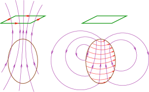
Figure 1: (COLOR) Schematic diagram of measurement and early time dynamics. Left: prior to pulse termination, transmitter coil currents generate a magnetic field in the neighborhood of the target. Right: just after pulse termination, the target interior has not had time to adjust to the absence of the transmitted field, and screening surface currents are generated to enforce the correct EM boundary conditions.

The early time response is governed by the dynamics of the screening currents, induced in response to the rapid quenching of the transmitted magnetic field immediately following pulse termination (see Fig. 1). The initial diffusion of these currents inward from the target surface generates a $t^{-1/2}$ power law in $V(t)$, with coefficient reflecting the surface properties of the target W03 . However, underlying this power law is the assumption that $t/\tau_{c}$ is the smallest parameter in the problem. It will now be shown that the background-target permeability contrast $\mu_{b}/\mu_{c}$ can generate a new small parameter that greatly limits the its range of validity. Specifically, an extended calculation is described that divides the early time regime $t<\tau_{e}$, where $\tau_{e}\ll\tau_{c}$ is the point at which bulk effects first begin to enter (see further below), into an early-early time regime, $0<t\ll\tau_{\rm mag}$, where the $V(t)\sim t^{-1/2}$ remains valid, and a late-early time regime $\tau_{\rm mag}\ll t\ll\tau_{e}$, where a new power law $V(t)\sim t^{-3/2}$ obtains. In the neighborhood of the magnetic crossover time,

$$\tau_{\rm mag}=\tau_{c}(\mu_{b}/\mu_{c})^{2},$$ (1)

an interpolation between the two power laws occurs (that is visible only if $\tau_{\rm mag}\ll\tau_{e}$), for which the full functional form is provided. For ferrous targets $\tau_{\rm mag}/\tau_{e}={\cal O}(10^{-4})$, and the early-early time regime is essentially invisible, and only the $t^{-3/2}$ behavior is seen, consistent with measured data: see Fig. 2.

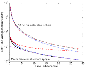
Figure 2: (COLOR) Geonics EM61-3D data (black curves) from nonmagnetic (aluminum) and ferrous (steel) targets, together with predicted exact solutions Jackson (blue curves). Asymptotic early-time power laws (red curves) are seen, with $t^{-1/2}$ for aluminum, $t^{-3/2}$ for steel. The former shows a crossover to multi-exponential decay behavior (magenta curve—the first 60 slowest decaying modes), consistent with $\tau_{e}={\cal O}(10^{-2}{\rm s})$, $\tau_{c}={\cal O}(10^{-1}{\rm s})$. The latter covers essentially the entire observed range, consistent with $\tau_{e}={\cal O}(10^{-5}{\rm s})$, $\tau_{c}={\cal O}(1\ {\rm s})$.

At low frequencies the dielectric function in the ground and in the target is dominated by the its imaginary part, $\epsilon=4\pi i\sigma/\omega$, where $\sigma({\bf x})$ is the dc conductivity, and the Maxwell equations may be reduced to a single equation for the vector potential,

$$\nabla\times\left(\frac{1}{\mu}\nabla\times{\bf A}\right)+\frac{4\pi\sigma}{c^{2}}\partial_{t}{\bf A}=\frac{4\pi}{c}{\bf j}_{S},$$ (2)

with magnetic induction ${\bf B}=\nabla\times{\bf A}$, field ${\bf H}={\bf B}/\mu$, and gauge chosen so that the electric field is ${\bf E}=-(1/c)\partial_{t}{\bf A}$. The transmitter loop generates the source current density ${\bf j}_{S}({\bf x},t)$. The conductivity and permeability are separated into background [$\sigma_{b}({\bf x})$, $\mu_{b}({\bf x})$] and conducting target [$\sigma_{c}({\bf x})$, $\mu_{c}({\bf x})$] components, where $\sigma_{c}$, $\mu_{c}$ vanish outside the target volume $V_{c}$. High conductivity contrast, $\sigma_{b}/\sigma_{c}\ll 1$, is required, but $\mu_{b}/\mu_{c}$ is arbitrary.

Equation (2) is a vector diffusion equation, with contrast $D_{b}/D_{c}={\cal O}(10^{7}\mbox{--}10^{9})$. The “background communication time” between instrument and target separated by distance $R$ is $\tau_{b}=R^{2}/D_{b}$. For representative values $\sigma_{b}=0.1$ S/m, $\mu_{b}=1$, $R=3$ m, one obtains $\tau_{b}={\cal O}(10^{-6}{\rm s})$, instantaneous even on the scale of $\tau_{r}$. Thus, the electrodynamics of the background may be treated as quasistatic: outside the target one may drop the $\partial_{t}{\bf A}$ term in (2). Further, following pulse termination ($t>0$) one has ${\bf j}_{S}\equiv 0$, hence $\nabla\times{\bf H}=0$, and one may derive ${\bf H}=-\nabla\Phi$ from a scalar potential $\Phi$, which in turn satisfies $\nabla\cdot(\mu_{b}\nabla\Phi)=0$. The external field is therefore entirely determined by the internal field through the boundary condition Jackson ${\bf\hat{n}}\cdot[\mu_{b}{\bf H}_{b}-\mu_{c}{\bf H}_{c}]=0$, where ${\bf H}_{b}$, ${\bf H}_{c}$ are the fields just outside and inside the target surface, and ${\bf\hat{n}}$ is the local surface normal. Thus, one obtains a Neumann-type boundary condition, $-{\bf\hat{n}}\cdot\nabla\Phi=(\mu_{c}/\mu_{b}){\bf\hat{n}}\cdot{\bf H}_{c}$, and hence the formal solution

$$\Phi({\bf x})=\int_{\partial V_{c}}d^{2}rg_{N}({\bf x},{\bf r})\frac{\mu_{c}}{\mu_{b}}{\bf\hat{n}}\cdot{\bf H}_{c}({\bf r}),$$ (3)

where $\partial V_{c}$ is the target surface, and $g_{N}$ is the Neumann Green function satisfying $-\mu_{b}^{-1}\nabla\cdot(\mu_{b}\nabla g_{N})=\delta({\bf x}-{\bf x}^{\prime})$ with boundary condition ${\bf\hat{n}}\cdot\nabla g_{N}=0$.

The initial surface screening current appears in the transverse magnetic boundary condition Jackson ; W03 : ${\bf K}({\bf r})=(c/4\pi){\bf\hat{n}}\times[{\bf H}_{b}({\bf r})-{\bf H}_{c}({\bf r})]$. As indicated in Fig. 1, ${\bf H}_{c}$ is the same as that prior to pulse termination, while ${\bf H}_{b}$ is given by (3):

$${\bf K}=-\frac{c}{4\pi}{\bf\hat{n}}\times(\nabla\Phi-{\bf H}_{c})_{t=0},$$ (4)

which, via (3), determines ${\bf K}$ entirely in terms of ${\bf H}_{c}$.

To investigate the evolution of ${\bf K}$ for $t>0$, we take advantage of the rapid variation of the fields near the surface with the local vertical coordinate $z$. Thus, $z$-derivatives dominate (2), and to leading order in the small parameter $\epsilon(t)=\sqrt{D_{c}t/L_{c}^{2}}$ foot1 , one obtains

$$-\partial_{Z}^{2}{\bf A}^{\perp}+\partial_{t}{\bf A}=0,\ z<0,$$ (5)

with initial condition ${\bf E}(0)=-(1/c)\partial_{t}{\bf A}(0)=\sigma_{c}^{-1}{\bf K}\delta(z)$. Here $Z=z/\sqrt{D_{c}}$, ${\bf A}^{\perp}={\bf A}-{\bf\hat{n}}({\bf\hat{n}}\cdot{\bf A})$ is the tangential part of ${\bf A}$, and $\mu,\sigma,D$ are treated as constants on either side of the boundary. One may choose $\Delta{\bf A}=0$ for $t=0$, and it follows immediately that ${\bf\hat{n}}\cdot\Delta{\bf A}\equiv 0$: $\Delta{\bf A}$ is purely transverse.

One requires now the boundary condition for (5) at $Z=0^{-}$. For $t>0$ let ${\bf A}={\bf A}(0)+\Delta{\bf A}(t)$ and $\Phi=\Phi(0)+\Delta\Phi(t)$, where one treats $|\Delta{\bf A}|/|{\bf A}(0)|,|\Delta\Phi|/|\Phi(0)|={\cal O}(\epsilon)$ and $|\partial_{Z}\Delta{\bf A}|/|\Delta{\bf A}|={\cal O}(1/\epsilon)$. Keeping only leading terms foot1 , continuity of ${\bf\hat{n}}\times{\bf H}$ (the surface current sheet now has finite thickness) and (4) imply that

$$\sqrt{\frac{4\pi\mu_{c}}{\sigma_{c}}}{\bf K}=-\partial_{Z}\Delta{\bf A}^{\perp}|_{Z=0^{-}}+\mu_{c}\sqrt{D_{c}}{\bf\hat{n}}\times\nabla\Delta\Phi|_{Z=0^{+}},$$ (6)

in which $\Delta\Phi$ is given by $\Delta{\bf A}(Z=0^{-})$ via (3). In fact, estimating $\partial_{Z}={\cal O}[D_{c}^{1/2}/\epsilon(t)L_{c}]$, $g_{N}={\cal O}(1/L_{c})$, and ${\bf\hat{n}}\times\nabla={\cal O}(1/L_{c})$, the ratio of the second term on the right hand side to the first is ${\cal O}[\epsilon(t)\mu_{c}/\mu_{b}]$. Their relative order is therefore time-dependent foot2 . In particular, at early-early time $\epsilon(t)\ll\mu_{b}/\mu_{c}$ (i.e., $t\ll\tau_{\rm mag}$) one may drop the second term. Lack of time dependence in ${\bf K}$ then leads to the simple homogeneous Neumann boundary condition $\partial_{z}{\bf E}=0$ for the electric field. This is the limit in which the early time analysis in Ref. W03 was carried out and the $t^{-1/2}$ behavior of $V(t)$ derived.

Thus, for $\mu_{c}/\mu_{b}={\cal O}(1)$ one gains nothing by including the $\Delta\Phi$ term: it is of the same order as other ${\cal O}[\epsilon(t)]$ terms previously dropped from (6) foot1 . However, if $\mu_{c}/\mu_{b}\gg 1$ this term dominates for $\tau_{\rm mag}<t<\tau_{e}$, which now comprises a large fraction of the early time regime. The remainder of this paper is concerned with extending the theory into this regime.

With the $\Delta\Phi$ term, (6) is nonlocal, coupling $\Delta{\bf A}(Z=0^{-})$ over the surface. In order to decouple (6) we diagonalize it by seeking transverse vector eigenfunctions ${\bm{\alpha}}_{n}$, $n=1,2,3,\ldots$, satisfying

$$\kappa_{n}{\bm{\alpha}}_{n}({\bf r})=-\mu_{c}\sqrt{D_{c}}{\bf\hat{n}}\times\nabla\psi_{n}({\bf r})$$ (7)

where $\kappa_{n}$ is the corresponding eigenvalue, and ${\bf r}$ is the surface coordinate. The scalar $\psi_{n}$ is defined by

$$\psi_{n}=\hat{\cal L}^{N}_{g}\mu_{b}^{-1}{\bf\hat{n}}\cdot\nabla\times{\bm{\alpha}}_{n},$$ (8)

where, to condense the notation, we define the Neumann Green function operator via $\hat{\cal L}^{N}_{g}\phi({\bf r})=\int_{\partial V_{c}}d^{2}r^{\prime}g_{N}({\bf r},{\bf r}^{\prime})\phi({\bf r}^{\prime})$. Substituting (7) into (8), one obtains a scalar eigenvalue problem,

$$\kappa_{n}\psi_{n}=\hat{\cal L}\psi_{n},\ \ \hat{\cal L}\equiv-\hat{\cal L}^{N}_{g}\mu_{b}^{-1}\hat{\cal L}_{\Delta},$$ (9)

where the generalized surface Laplacian is $\hat{\cal L}_{\Delta}\phi({\bf r})={\bf\hat{n}}\cdot\nabla\times\left[\mu_{c}\sqrt{D_{c}}{\bf\hat{n}}\times\nabla\phi({\bf r})\right]$. On a sphere one obtains $\hat{\cal L}_{\Delta}=-\mu_{c}\sqrt{D_{c}}L_{c}^{-2}{\bf L}^{2}$, where $L_{c}$ is now the radius, and ${\bf L}=-i{\bf x}\times\nabla$ is the angular momentum operator Jackson .

As the ${\bm{\alpha}}_{n}$ are derived from the scalar $\psi_{n}$ via (7), they do not form a complete set of 2D vector fields. The missing fields consist of the kernel of (7) (the space of functions $\kappa_{n}=0$), spanned by all fields ${\bm{\beta}}$ with vanishing normal magnetic field, ${\bf\hat{n}}\cdot\nabla\times{\bm{\beta}}=0$. It follows that ${\bm{\beta}}=-\nabla^{\perp}\phi\equiv{\bf\hat{n}}\times{\bf\hat{n}}\times\nabla\phi$ for some other scalar $\phi$. Let $\phi_{n}$, ${\bm{\beta}}_{n}$ be chosen as eigenfunctions of the generalized transverse Laplace equation,

$$\lambda_{n}\phi_{n}({\bf r}) = -{\bf\hat{n}}\cdot\nabla\times\left[\mu_{c}^{-1}D_{c}^{-1/2}{\bf\hat{n}}\times\nabla\phi_{n}({\bf r})\right]$$

$${\bm{\beta}}_{n}({\bf r}) = -\nabla^{\perp}\phi_{n},$$ (10)

with a new set of eigenvalues $\lambda_{n}$.

The set $\{{\bm{\alpha}}_{n},{\bm{\beta}}_{n}\}$ forms a complete basis, and we perform the magnetic surface mode expansion

$$\Delta{\bf A}({\bf x},t) = \sum_{n=1}^{\infty}\left[A^{(1)}_{n}(Z,t){\bm{\alpha}}({\bf r})+A^{(2)}_{n}(Z,t){\bm{\beta}}({\bf r})\right]$$

$$\sqrt{\frac{4\pi\mu_{c}}{\sigma_{c}}}{\bf K}({\bf r}) = \sum_{n=1}^{\infty}\left[K^{(1)}_{n}{\bm{\alpha}}({\bf r})+K^{(2)}_{n}{\bm{\beta}}({\bf r})\right].$$ (11)

From (7), $\hat{\cal L}_{g}^{N}\mu_{b}^{-1}{\bf\hat{n}}\cdot\nabla\times\Delta{\bm{A}}=\sum_{n}A^{(1)}_{n}\psi_{n}$, and from (10), ${\bf\hat{n}}\cdot\nabla\times(\mu_{c}^{-1}D_{c}^{-1/2}\Delta{\bf A})=\sum_{n}\lambda_{n}A^{(2)}_{n}\phi_{n}$ (and similarly for ${\bf K}$), hence appropriate orthogonality relations for $\psi_{n},\phi_{n}$ may be used to determine $A_{n}^{(i)},K_{n}^{(i)}$.

Substituting (11) into (5) and (6), complete separation of the surface modes is achieved:

$$(\partial_{t}-\partial_{Z}^{2})A^{(i)}_{n}=0,\ Z<0,$$ (12)

with initial and boundary conditions

$$-\partial_{t}A^{(i)}_{n}|_{t=0^{+}} = K^{(i)}_{n}\delta(Z)$$

$$(\partial_{Z}+\kappa_{n}\delta_{i1})A^{(i)}_{n}|_{Z=0^{-}} = -K^{(i)}_{n}.$$ (13)

The solutions are $A^{(i)}_{n}(Z,t)=-K^{(i)}_{n}H(Z,t;\kappa_{n}\delta_{i1})$, where

$$H(Z,t;\kappa) = \textstyle\frac{1}{\kappa}\left[{\rm erfc}\left(\frac{|Z|}{\sqrt{4t}}\right)-e^{\kappa^{2}t-\kappa Z}{\rm erfc}\left(\frac{2\kappa t-Z}{\sqrt{4t}}\right)\right]$$

$$H(Z,t;0) = \textstyle\sqrt{\frac{4t}{\pi}}e^{-Z^{2}/4t}-|Z|{\rm erfc}\left(\frac{|Z|}{\sqrt{4t}}\right),$$ (14)

where ${\rm erfc}(x)$ is the complementary error function.

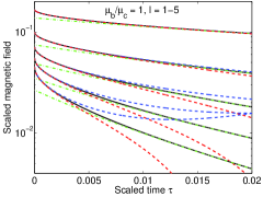
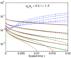
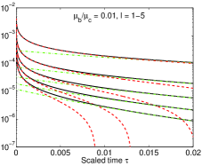
Figure 3: (COLOR) Comparison between exact and early time results for spheres in a homogeneous background. Plotted is $H_{l}(\tau\equiv t/\tau_{c})$ for $1\leq l\leq 5$ (curves for higher values of $l$ lie lower on the plots). Left: $\mu_{c}/\mu_{b}=1$. Blue (dashed) lines show the asymptotic early-early-time form (19); red (dashed) lines show the full early time solution; black (solid) lines show exact results; and green (dash-dotted) lines show (21) truncated at the first 3 terms (an approximation that might emerge from a late time perturbative approach WL03 ). The two early time curves, though differing in detail, exhibit roughly the same accuracy, with interval of validity shrinking as $L_{lm}/L_{c}=1/l^{2}$, as predicted. In realistic applications, the transmitted field in the target region will be fairly uniform, and one may expect $l=1$ to dominate, with small corrections from higher $l$. The union of early and late time approximations then provide a rather accurate description of the full signal. Center: $\mu_{c}/\mu_{b}=5$. The full early time form now clearly exhibits greatly extended accuracy over the early-early time power law. Right: $\mu_{c}/\mu_{b}=100$. The full early-time form is indistinguishable from the late-early time form (19), the early-early time interval being invisibly narrow.

Fields external to the target are obtained by extending ${\bm{\alpha}}_{n},{\bm{\beta}}_{n}$ into the exterior space. First, let

$$\psi_{n}({\bf x}) = -\frac{1}{\kappa_{n}}\int_{\partial V_{c}}d^{2}r^{\prime}g_{N}({\bf x},{\bf r}^{\prime})\frac{1}{\mu_{b}}\hat{\cal L}_{\Delta}\psi_{n}({\bf r}^{\prime})$$

$$\phi_{n}({\bf x}) = \int_{\partial V_{c}}d^{2}r^{\prime}g_{D}({\bf x},{\bf r}^{\prime})\phi_{n}({\bf r}^{\prime}),$$ (15)

in which $g_{D}({\bf x},{\bf x}^{\prime})$ is the Dirichlet Green function satisfying $-\sigma_{b}^{-1}\nabla\cdot(\sigma_{b}\nabla g_{D})=\delta({\bf x}-{\bf x}^{\prime})$ and vanishing on $\partial V_{c}$, and ${\bf x}$ is no longer restricted to the surface. These definitions guaranteed continuity at the boundary. The vector eigenfunctions are now extended by solving

$$\mu_{b}\nabla\times{\bm{\alpha}}_{n}({\bf x})=-\nabla\psi_{n}({\bf x}),\ \nabla\cdot(\sigma_{b}{\bm{\alpha}}_{n})=0,$$ (16)

while imposing continuity of ${\bm{\alpha}}^{\perp}_{n}$ at the surface, and

$${\bm{\beta}}_{n}({\bf x})=-\nabla\phi_{n}({\bf x}).$$ (17)

Since $\nabla\times{\bm{\beta}}_{n}=0$ it does not contribute to the external magnetic field, and hence to any inductive measurement. The external field is now simply

$$\Delta{\bf A}({\bf x},t)=\sum_{n=1}^{\infty}\left[A^{(1)}_{n}(0^{-},t){\bm{\alpha}}_{n}({\bf x})+A^{(2)}_{n}(0^{-},t){\bm{\beta}}_{n}({\bf x})\right],$$ (18)

with time-dependence given by the internal field on the boundary, hence governed by the function

$$H(0,t;\kappa)=\frac{1}{\kappa}\left[1-e^{\kappa^{2}t}{\rm erfc}\left(\kappa\sqrt{t}\right)\right]$$ (19)

$$\to\begin{cases}\sqrt{\frac{4t}{\pi}}\left[1-\frac{1}{2}(\pi\kappa^{2}t)^{1/2}+{\cal O}(\kappa^{2}t)\right],&\kappa^{2}t\ll 1\\ \frac{1}{\kappa}\left\{1-(\pi\kappa^{2}t)^{-1/2}+{\cal O}[(\kappa^{2}t)^{-3/2}]\right\}&\kappa^{2}t\gg 1.\end{cases}$$

The time derivative, entering the electric field and voltage, displays the promised $t^{-1/2}$ and $t^{-3/2}$ power laws in the two limits. If $\psi_{n}$ varies on scale $L_{n}\leq L_{c}$, one may estimate from (9) $\kappa_{n}={\cal O}[\tau_{\rm mag}^{-1/2}(L_{c}/L_{n})]$, hence crossover point $\tau_{{\rm mag},n}\equiv 1/\kappa_{n}^{2}={\cal O}[\tau_{\rm mag}(L_{n}/L_{c})^{2}]$. One expects $L_{n}=L_{c}$ only for the fundamental mode, hence (1) actually represents an upper bound on the spectrum of crossover times $\tau_{{\rm mag},n}$.

The exact solution for a homogeneous sphere in a homogeneous background serves to clarify all of the above concepts. The operators $\hat{\cal L}_{g}^{N}$ and $\hat{\cal L}_{\Delta}$ now commute and may be simultaneously diagonalized using spherical harmonics: $\hat{\cal L}_{g}^{N}Y_{lm}=Y_{lm}/(l+1)L_{c}$, $\hat{\cal L}_{\Delta}Y_{lm}=-[\mu_{c}\sqrt{D_{c}}l(l+1)/L_{c}^{2}]Y_{lm}$. Thus, using $\psi_{lm}=\phi_{lm}=L_{c}^{-2}Y_{lm}$ one obtains $\kappa_{lm}=l\tau_{\rm mag}^{-1/2}$ (hence mode length scale $L_{lm}=L_{c}/l$), and $\lambda_{lm}=l(l+1)/L_{c}^{2}\mu_{c}\sqrt{D_{c}}$. The vector functions are ${\bm{\alpha}}_{lm}({\bf x})=-i\mu_{b}\sqrt{(l+1)/l}(L_{c}^{l}/x^{l+1}){\bf X}_{lm}$, ${\bm{\beta}}_{lm}({\bf x})=-i\sqrt{(l+1)/l}\nabla\times[(L_{c}^{l}/x^{l+1}){\bf X}_{lm}]$, where ${\bf X}_{lm}=[l(l+1)]^{-1/2}{\bf\hat{L}}Y_{lm}$ are the vector harmonics Jackson . The exact solution associated with the magnetic modes ${\bm{\alpha}}_{lm}$ is governed by the usual bulk exponentially decaying mode expansion WL03 ; W03 , from which one obtains $A_{lm}^{(1)}(t)=K^{(1)}_{lm}\sqrt{4\tau_{c}}[H_{l}(0)-H_{l}(t/\tau_{c})]$, where

$$H_{l}(\tau)=\sum_{n=1}^{\infty}\frac{j_{l}(\zeta_{ln})^{2}}{j_{l}(\zeta_{ln})^{2}-j_{l+1}(\zeta_{ln})j_{l-1}(\zeta_{ln})}\frac{e^{-\zeta_{ln}^{2}\tau}}{\zeta_{ln}^{2}},$$ (20)

where $j_{l}(x)$ are the spherical Bessel functions, and the scaled decay rates are given by the roots of

$$0=\frac{\mu_{b}}{\mu_{c}}\zeta_{ln}j_{l-1}(\zeta_{ln})+l\left(1-\frac{\mu_{c}}{\mu_{b}}\right)j_{l}(\zeta_{ln}).$$ (21)

In Fig. 3 $H_{l}(t/\tau_{c})$ is compared to the early time prediction $H_{l}(t/\tau_{c})\approx H_{l}(0)-(4\tau_{c})^{-1/2}H(0^{-},t;\kappa_{lm})$, with $H_{l}(0)=(\mu_{b}/2\mu_{c})/[l+(l+1)\mu_{b}/\mu_{c}]$, for various $l$, $\mu_{c}/\mu_{b}$.

The author is indebted to E. M. Lavely for numerous discussions. The support of SERDP, through contract No. DACA 72-02-C-0029, is gratefully acknowledged.

References

(1) See, e.g.,
http://www.serdp.org/research/research.html for a list of ongoing
projects in these areas.
(2) See, e.g., C. V. Nelson and
T. B. Huynh, “Wide bandwidth time decay responses from low metal
mines and ground voids,” in Proc. SPIE Vol. 4394
Detection and Remediation Technologies for Mines and
Minelike Targets VI, (SPIE, Bellingham, WA, 2001), p. 55.
(3) P. B. Weichman and E. M. Lavely in Detection
and Remediation Technologies for Mines and Minelike Targets VIII,
SPIE Proc. Vol. 5089 (SPIE–International Society for Opitcal
Engineering, Bellingham, WA, 2003), p. 1189.
(4) P. B. Weichman, Phys. Rev. Lett. 91, 143908
(2003).
(5) See, e.g., J. D. Jackson, Classical
Electrodynamics (John Wiley and Sons, New York, 1975).
(6) Specifically transverse derivative terms in
, as well as
derivatives of with respect to that arise in
the change of variable from to , all estimated to be of
rather than , are
dropped in both (5) and (6).
(7) Establishing that there are no other terms
contributing to (6) at leading order for arbitrary values of
is nontrivial, and requires a very careful estimate
of all possible higher order terms [P. B. Weichman, unpublished].