Phase Shifts and Resonances in the Dirac Equation

CUQM-103
                                                                                                             math-ph/0401015
                                                                                                             January 2004

Phase Shifts and Resonances in the Dirac Equation
Piers Kennedy ^∗a, Richard L. Hall ^+b, and Norman Dombey ^†a

^aCentre for Theoretical Physics, University of Sussex, Brighton BN1 9QJ, UK
            ^bDepartment of Mathematics and Statistics, Concordia University, Montreal, Quebec, H3G 1M8, Canada
            ^∗email: kapv4@sussex.ac.uk   ⁺email: rhall@mathstat.concordia.ca   ^†email: normand@sussex.ac.uk

Abstract

We review the analytic results for the phase shifts $\delta_{l}(k)$ in non-relativistic scattering from a spherical well. The conditions for the existence of resonances are established in terms of time-delays. Resonances are shown to exist for p-waves (and higher angular momenta) but not for s-waves. These resonances occur when the potential is not quite strong enough to support a bound p-wave of zero energy. We then examine relativistic scattering by spherical wells and barriers in the Dirac equation. In contrast to the non-relativistic situation, s-waves are now seen to possess resonances in scattering from both wells and barriers. When s-wave resonances occur for scattering from a well, the potential is not quite strong enough to support a zero momentum s-wave solution at $E=m$. Resonances resulting from scattering from a barrier can be explained in terms of the ‘crossing’ theorem linking s-wave scattering from barriers to p-wave scattering from wells. A numerical procedure to extract phase shifts for general short range potentials is introduced and illustrated by considering relativistic scattering from a Gaussian potential well and barrier.

Introduction

The question of what does or does not constitute a resonance in potential scattering still seems to cause some confusion. Many authors who consider scattering in simple systems such as the one-dimensional square well in the Schrödinger equation talk of transmission ‘resonances’ when the transmission coefficient $T=1$ with little or no justification as to why these might be resonances. It would seem on the surface that a resonance exists on account of a maximum or peak in a measure of the scattering (for example the transmission coefficient in one dimension or the cross-section for a particular partial wave in three dimensions). But Wigner [1] pointed out nearly 50 years ago that in order to have a true physical resonance the scattered particle must be captured in some way by the scattering centre. So in addition to the peak in the scattering probability function, there must also be a delay in the transition time of the particle through the target: this requirement is fulfilled by demanding that the Wigner time delay is positive. This implies that the phase shift associated with the peak must increase through an odd multiple of $\frac{\pi}{2}$ as the particle energy increases through the resonance energy.

We will begin this paper by looking at the phase shifts for the simple case of scattering from a spherical well in the Schrödinger equation in order to illustrate resonant behaviour and distinguish it from cases where the cross-section peaks but there is no resonance. The argument and results closely follow those given by Newton [2]. It will be seen that, using Wigner’s criteria, the spherical well does not give rise to s-wave resonances. Resonances do exist, however, for scattered p-waves and waves of higher angular momenta. This comes about because of the centrifugal term in the Schrödinger equation for partial waves $l>0$.

The relationship between bound states and continuum states for non-relativistic systems is well documented. Schiff [3] noted that ‘a potential well that has an energy level nearly at zero exhibits a resonance in the low-energy scattering of particles with the same $l$ value as the energy level’. Newton [2] later studied this more carefully and showed that one can go smoothly from a zero energy solution to a real resonance by weakening the potential slightly. This idea is crucial to the the procedure we will adopt. First the condition on the potential to support a zero energy solution must be established. This condition can then be relaxed slightly to push the solution into a continuum state. Finally the phase shift corresponding to the resulting peak in cross-section is checked to see if it fulfils the criterion of positive time delay necessary for a real resonance.

In this paper we generalise these results to the relativistic Dirac equation in three dimensions. We begin by reproducing the results for the phase shift in the spherical potential well and analyse whether resonant behaviour exists. In contrast to the non-relativistic results it will be shown that scattered s-waves do now give rise to resonances. It will be shown that these arise because of the presence of a centrifugal term in the original coupled equations which does not disappear even for s-waves. But we cannot stop there: in the Dirac equation we must consider the zero momentum solutions which exist at both $E=m$ and $E=-m$. We refer to these as critical solutions and in particular it is conventional to refer to the solution at $E=-m$ as supercritical. It will be shown that a ‘crossing theorem’ exists which connects scattering of particles by potential barriers to the supercritical state at $E=-m.$ This phenomenon was first illustrated in a previous paper by two of us [4] in the context of positron-heavy nuclei scattering. We use this theorem to show that resonances exist in s-wave Dirac scattering from spherical barriers as well as spherical wells. Resonances also occur in higher partial waves as expected.

We then investigate resonant scattering by general short range spherically-symmetric potential wells and barriers in the Dirac equation. A numerical procedure for the extraction of the phase shifts is demonstrated in the case of a Gaussian potential wells and barriers, and the results are analysed. We demonstrate that s-wave resonances can exist in scattering by both barriers and wells.

The Schrödinger equation

The phase shifts $\delta_{l}(k)$ for the spherical well $V(r)=-V$ $r\leq a;$ $V(r)=0$ $r>a$ are well known [3], [5]:

$$\tan\delta_{l}=\frac{k\,j_{l}^{\prime}(ka)j_{l}(pa)-p\,j_{l}(ka)j_{l}^{\prime}(pa)}{k\,n_{l}^{\prime}(ka)j_{l}(pa)-p\,n_{l}(ka)j_{l}^{\prime}(pa)}$$ (1)

where $j_{l}$ and $n_{l}$ are the regular and irregular spherical Bessel functions respectively, $k^{2}=2mE$ and $p^{2}=2m(E+V)$. So for s-wave scattering when $l=0$ this becomes:

$$\tan\delta_{0}=\frac{k\tan pa-p\tan ka}{p+k\tan ka\tan pa}$$ (2)

while for p-wave scattering when $l=1$ this gives:

$$\tan\delta_{1}=\frac{akp^{2}\tan pa-ak^{2}p\tan ka+(k^{2}-p^{2})\tan ka\tan pa}{ak^{2}p+(p^{2}-k^{2})\tan pa+akp^{2}\tan ka\tan pa}$$ (3)

The potential wells of the greatest interest are those which are not quite deep enough to support a bound state. The critical values of the potential well which support states of zero energy (these may or may not be bound - this will be discussed later) are well established [3]. For $l=0$ we have

$$j_{0}(pa)=pa\,j_{1}(pa)\\ \Rightarrow\quad\cos\,pa=0\quad\Rightarrow V_{c}=\frac{(2n-1)^{2}\pi^{2}}{8ma^{2}}$$ (4)

and for $l>0$ we have

$$j_{l-1}(pa)=0$$ (5)

For $l=1$ this leads to

$$\sin\,pa=0\quad\Rightarrow\quad V_{c}=\frac{n^{2}\pi^{2}}{2ma^{2}}$$ (6)

We are now in a position to examine the low energy phase shift behaviour in order to see if resonances occur. In the case of the s-wave, if the potential is not quite strong enough to bind the first state, the phase shift $\delta_{0}(k)$ will be seen to rise from zero but never quite reach the value $\frac{\pi}{2}$ before it decreases for larger energies. If we continue to increase the strength of the potential well there will be a value at which the phase shift at zero energy $\delta_{0}(0)$ flips from zero to $\frac{\pi}{2}$. The strength at this point is exactly the critical value $V=V_{c}$ from Eq. (4), required for the potential to just support the first $l=0$ critical state. As soon as we just increase the strength of the potential from $V_{c}$, $\delta_{0}(0)$ flips to the value $\pi$ and decreases for increasing energy. This behaviour is illustrated in the following figure:

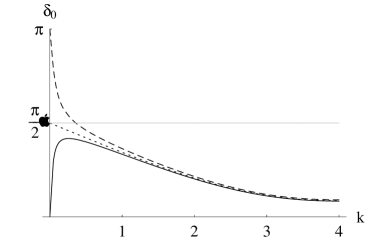
FIG. 1.: The s-wave phase shifts for the spherical well. A zero-energy state exists for a potential of strength $V_{c}=0.25\pi^{2}\approx 2.47$ (dotted line). The solid line represents a potential of strength $V=2.4$ which almost binds whilst the dashed line is the potential of strength $V=2.6$ which contains a loosely bound state. ($a=1$ and $m=0.5$).

The process repeats with every additional bound state, so $\delta_{0}(0)$ increases by $\pi$ each time and we have Levinson’s theorem:

$$\delta_{0}(0)=n_{0}\pi$$ (7)

where $n_{0}$ tells us the number of $l=0$ bound states. For critical values of the potential when it is just strong enough to possess a zero-energy state, Levinson’s theorem must be modified to

$$\delta_{0}(0)=(n_{0}+\displaystyle\frac{1}{2})\pi$$ (8)

Although it is not obvious, the critical state is not actually bound but instead forms part of the continuum. In order to see this consider the Schrödinger equation with for a potential well:

$$\Psi^{\prime\prime}(r)-\left[\frac{l(l+1)}{r^{2}}+2mV(r)-k^{2}\right]\Psi(r)=0$$ (9)

If the potential vanishes faster than $1/r^{2}$ at large distances, the zero-energy solution for large $r$ is found from

$$\Psi^{\prime\prime}(r)\approx\frac{l(l+1)}{r^{2}}\Psi(r)$$ (10)

Consequently $\Psi$ behaves as $1/r^{l}$ at infinity and the particle will only be normalisable, hence bound, for $l>0$. This means that for the first critical value of the potential, $V=V_{c}=\pi^{2}/4$ when $l=0$, the state is not bound, $n_{0}=0$ and $\delta_{0}(0)=\frac{\pi}{2}$ from (8). These states are often referred to as half-bound states [2].

In order for a resonance to exist the Wigner time delay must be positive. This is defined as

$$\tau_{l}=2\frac{d\delta_{l}}{dE}=\frac{2}{v}\frac{d\delta_{l}}{dk}$$ (11)

So the phase shift must increase through $\pi/2$. A decrease in the phase shift as the energy increases through $\pi/2$ gives rise to a negative time delay - a time advancement [6]. This does not constitute a resonance. Hence there are no s-wave resonances for a spherical well.

The results for p-waves (and other higher angular momentum waves) are distinctly different. If the potential is not quite strong enough to bind the first state, the phase shift $\delta_{1}(k)$ rises from zero but it now increases through the value $\frac{\pi}{2}$ at some positive value of the energy up to a maximum value ($<\pi$) before decreasing for larger energies. If we continue to increase the strength of the potential, the maximum of the phase shift approaches the value $\pi$ for decreasing values of the energy until the phase shift at zero energy $\delta_{1}(0)$ flips from zero to $\pi$. The strength of the potential at this point is exactly the critical value $V_{c}=\pi^{2}$ from (6), required for the potential to just support the first $l=1$ bound state. It should be noted that, contrary to the s-wave case, the critical wave functions are bound states.

To illustrate that there are p-wave resonances but no s-wave resonances, we can consider the effective potential $V_{eff}(r)=V(r)+l(l+1)/r^{2}$ shown in figure 2.

FIG. 2.: The effective potential for a spherical well.

For $l=0$ there is no centrifugal barrier to trap the particle for small positive energies and consequently low momentum resonances do not occur. At zero energy there is nothing to stop the particle escaping the well - it is not bound and forms part of the continuum. For angular momenta $l>0$, there is now a barrier which can momentarily trap particles giving rise to a resonance in the physical region $E>0$. If we scatter a particle of energy $E<l(l+1)/a^{2}$ (i.e. below the lip of the repulsive centrifugal barrier - see figure 2), it can tunnel into the target and once there eventually leak back out. If we deepen the potential the particle becomes increasingly trapped as the strength of the barrier through which it must tunnel increases and the resonance becomes more pronounced as it is retarded for greater lengths of time. We finally arrive at the critical value of the potential for which $E=0$ and the particle is completely trapped provided $l>0.$

As we continue to increase the strength of the potential beyond this critical value $\delta_{l}(0)$ jumps by $\pi$ for each additional bound state as is the case for $l=0$. For $l>0$ there are no half-bound states so Eq. (8) is no longer applicable and Eq. (7) can be modified to

$$\delta_{l}(0)=n_{l}\pi$$ (12)

where $n_{l}$ now tells us the number of bound states with angular momentum $l$. From figure (3) we can see that the phase shift associated with potentials which almost contain a bound state will increase through an odd multiple of $\frac{\pi}{2}$. As we get closer to criticality the phase shift increases more and more rapidly through this value and will peak at values that tend to $0$ (mod $\pi$). This manifests itself as an increasingly more pronounced peak in the cross-section.

This behaviour is illustrated in figure 3. The solid line represents a potential of strength $V=9$ and the dashed line represents a potential of strength $V=9.7$, where both potentials are just too weak to have a bound state. The dotted line is a potential of strength $V=10$ which contains a loosely bound state. A zero-energy $l=1$ bound state exists for a potential well of strength $V_{c}=\pi^{2}\approx 9.87$. ($a=1$ and $m=0.5$).

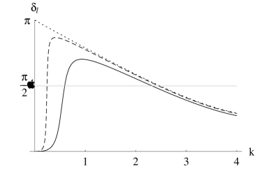
FIG. 3.: The spherical well for p-wave phase shifts.

The Dirac Equation : Scattering Solutions

We will now consider the problem of scattering from a spherical well in the relativistic Dirac equation. Following Greiner, Müller and Rafelski [7], which we refer to as GMR, the coupled radial equations for an electron of mass $m$ and energy $E$ in the presence the spherical well $V(r)=-V$ $r\leq a;$ $V(r)=0$ $r>a$ can be written

$$f^{\prime}(r) = -\frac{\chi}{r}f(r)+(E+m+V)g(r)$$ (13)

$$g^{\prime}(r) = -(E-m+V)f(r)+\frac{\chi}{r}g(r)$$ (14)

where the Dirac wave function $\Psi(r)$ for the radial equation is given by $r\Psi(r)=\left(\begin{array}[]{c}f\\ g\end{array}\right)$ The variable $\chi=\pm(j+\frac{1}{2})=\pm 1,\pm 2,...$ with the orbital angular momentum $l=j+\frac{1}{2}\frac{\chi}{|\chi|}=${$0,1,2,..$} corresponding to {$s,p,d,..$} waves. When $r<a$, the solutions are

$$f(r) = a_{1}rj_{l_{\chi}}(pr)$$ (15)

$$g(r) = a_{1}\frac{\chi}{|\chi|}\frac{pr}{E+V+m}j_{l_{-\chi}}(pr)$$ (16)

where the well momentum $p$ is

$$p^{2}=(E+V)^{2}-m^{2}$$ (17)

and

$$l_{\chi}=\left\{\begin{array}[]{lr}\chi&\qquad\chi>0\\ -\chi-1&\qquad\chi<0\end{array}\right.\qquad,\qquad l_{-\chi}=\left\{\begin{array}[]{lr}-\chi&\qquad-\chi>0\\ \chi-1&\qquad-\chi<0\end{array}\right.$$ (18)

When $r>a$, the free particle solutions are:

$$f(r) = b_{1}rj_{l_{\chi}}(kr)+b_{2}rn_{l_{\chi}}(kr)$$ (19)

$$g(r) = \frac{\chi}{|\chi|}\frac{kr}{E+m}[b_{1}j_{l_{-\chi}}(kr)+b_{2}n_{l_{-\chi}}(kr)]$$ (20)

where $k^{2}=E^{2}-m^{2}$. When $r\to\infty$ the following asymptotic forms for the spherical Bessel functions are required:

$$x\,j_{n}(x)\sim \sin\left(x-\frac{n\pi}{2}\right)\qquad\qquad x\,n_{n}(x)\sim -\cos\left(x-\frac{n\pi}{2}\right)$$ (21)

The components can therefore be written as

$$f(r) \to \frac{1}{k}\left[b_{1}\sin\left(kr-\frac{l_{\chi}\pi}{2}\right)-b_{2}\cos\left(kr-\frac{l_{\chi}\pi}{2}\right)\right]$$ (22)

$$g(r) \to \frac{\chi}{|\chi|}\frac{1}{E+m}\left[b_{1}\sin\left(kr-\frac{l_{-\chi}\pi}{2}\right)-b_{2}\cos\left(kr-\frac{l_{-\chi}\pi}{2}\right)\right]$$ (23)

Therefore

$$f(r) \to \frac{b_{1}}{|b_{1}|}\frac{A}{k}\sin\left(kr-\frac{l_{\chi}\pi}{2}+\delta_{l_{\chi}}\right)$$ (24)

$$g(r) \to \frac{b_{1}}{|b_{1}|}\frac{\chi}{|\chi|}\frac{A}{E+m}\sin\left(kr-\frac{l_{-\chi}\pi}{2}+\delta_{l_{\chi}}\right)$$ (25)

where

$$A\cos\delta_{l_{\chi}}=b_{1}\qquad\qquad A\sin\delta_{l_{\chi}}=-b_{2}$$ (26)

So

$$\tan\delta_{l_{\chi}}=-\frac{b_{2}}{b_{1}}\qquad\qquad A^{2}=b_{1}^{2}+b_{2}^{2}$$ (27)

This relationship between the phase shifts and the coefficients $b_{1}$ and $b_{2}$ was shown for s-waves by GMR. Depending on the sign of $\chi$ we have

$$l_{-\chi}=\left\{\begin{array}[]{l}l_{\chi}+1\qquad\chi<0\\ l_{\chi}-1\qquad\chi>0\end{array}\right.\qquad\qquad l_{\chi}-l_{-\chi}=\frac{\chi}{|\chi|}$$ (30)

Using the above together with Eqs. (24 and 25), the two components are found to be

$$f(r) \to \frac{b_{1}}{|b_{1}|}\frac{A}{k}\sin\left(kr-\frac{l_{\chi}\pi}{2}+\delta_{l_{\chi}}\right)$$ (31)

$$g(r) \to \frac{b_{1}}{|b_{1}|}\frac{A}{E+m}\cos\left(kr-\frac{l_{\chi}\pi}{2}+\delta_{l_{\chi}}\right)$$ (32)

The asymptotic forms are clearly dependent on the sign of $\chi$:

$$r\Psi(r)=\left(\begin{array}[]{c}f(r)\\ g(r)\end{array}\right)\to\frac{b_{1}}{|b_{1}|}A\left(\begin{array}[]{c}\frac{\displaystyle 1}{\displaystyle k}\cos\left(kr+\frac{\chi\pi}{2}+\delta_{l_{\chi}}\right)\\[5.69046pt] -\frac{\displaystyle 1}{\displaystyle E+m}\sin\left(kr+\frac{\chi\pi}{2}+\delta_{l_{\chi}}\right)\end{array}\right)\qquad\qquad\chi<0$$ (33)

$$r\Psi(r)=\left(\begin{array}[]{c}f(r)\\ g(r)\end{array}\right)\to\frac{b_{1}}{|b_{1}|}A\left(\begin{array}[]{c}\frac{\displaystyle 1}{\displaystyle k}\sin\left(kr-\frac{\chi\pi}{2}+\delta_{l_{\chi}}\right)\\[5.69046pt] \frac{\displaystyle 1}{\displaystyle E+m}\cos\left(kr-\frac{\chi\pi}{2}+\delta_{l_{\chi}}\right)\end{array}\right)\qquad\qquad\chi>0$$ (34)

These results are consistent with Barthélémy [8], [9]. We can combine Eqs. (20) and (27) to incorporate the phase shift into the free-particle wave components of the wave function:

$$f(r) = b_{1}r[j_{l_{\chi}}(kr)-\tan\delta_{l_{\chi}}n_{l_{\chi}}(kr)]$$ (35)

$$g(r) = \frac{\displaystyle\chi}{\displaystyle|\chi|}\frac{\displaystyle kr}{\displaystyle E+m}b_{1}[j_{l_{-\chi}}(kr)-\tan\delta_{l_{\chi}}n_{l_{-\chi}}(kr)]$$ (36)

The solutions for $r<a$ from Eqs. (14) and $r>a$ from Eqs. (36) must be joined smoothly; by dividing the top component by the bottom component and equating the two solutions at $r=a$ we arrive at

$$\frac{a_{1}j_{l_{\chi}}(pa)}{\frac{\chi}{|\chi|}\frac{p}{E+V+m}a_{1}j_{l_{-\chi}}(pa)}=\frac{b_{1}[j_{l_{\chi}}(ka)-\tan\delta_{l_{\chi}}n_{l_{\chi}}(ka)]}{\frac{\chi}{|\chi|}\frac{k}{E+m}b_{1}[j_{l_{-\chi}}(ka)-\tan\delta_{l_{\chi}}n_{l_{-\chi}}(ka)]}$$ (37)

After re-arrangement this becomes

$$\frac{k}{p}\,\frac{E+V+m}{E+m}\,\frac{j_{l_{\chi}}(pa)}{j_{l_{-\chi}}(pa)}=\frac{j_{l_{\chi}}(ka)-\tan\delta_{l_{\chi}}n_{l_{\chi}}(ka)}{j_{l_{-\chi}}(ka)-\tan\delta_{l_{\chi}}n_{l_{-\chi}}(ka)}$$ (38)

Taking $p=\sqrt{(E+V)^{2}-m^{2}}$ we find that the kinematic term $\gamma$ is given by

$$\gamma=\frac{p}{k}\,\frac{E+m}{E+V+m}$$ (39)

Solving for $\tan\delta_{l_{\chi}}$ we find that the relativistic equivalent of the Schrödinger result (1) is

$$\tan\delta_{l_{\chi}}=\frac{\gamma j_{l_{\chi}}(ka)j_{l_{-\chi}}(pa)-j_{l_{\chi}}(pa)j_{l_{-\chi}}(ka)}{\gamma j_{l_{-\chi}}(pa)n_{l_{\chi}}(ka)-j_{l_{\chi}}(pa)n_{l_{-\chi}}(ka)}$$ (40)

The Dirac Equation : Zero Momentum Solutions

In this section we establish the critical solutions for the spherical well. Unlike the previous non-relativistic situation, the Dirac equation has two critical solutions corresponding to $E=m$ and $E=-m$; the analysis which follows allows us to consider both of these critical solutions. For the spherical well potential the coupled radial Eqs. (14) have the solutions inside the well:

$$f(r) = r[a_{1}j_{l_{\chi}}(pr)+a_{2}n_{l_{\chi}}(pr)]$$ (41)

$$g(r) = \frac{\chi}{|\chi|}\frac{pr}{E+V+m}[a_{1}j_{l_{-\chi}}(pr)+a_{2}n_{l_{-\chi}}(pr)]$$ (42)

and the solutions outside the well are

$$f(r) = r\sqrt{\frac{2\kappa r}{\pi}}[b_{1}K_{l_{\chi}+\frac{1}{2}}(\kappa r)+b_{2}I_{l_{\chi}+\frac{1}{2}}(\kappa r)]$$ (43)

$$g(r) = \frac{\kappa r}{E+m}\sqrt{\frac{2\kappa r}{\pi}}[-b_{1}K_{l_{-\chi}+\frac{1}{2}}(\kappa r)+b_{2}I_{l_{-\chi}+\frac{1}{2}}(\kappa r)]$$ (44)

where $\kappa^{2}=m^{2}-E^{2}$. $K_{n+\frac{1}{2}}(\kappa r)$ and $I_{n+\frac{1}{2}}(\kappa r)$ are the modified spherical Bessel functions. In order to establish the bound states the internal wave function must be normalisable at the origin therefore $a_{2}=0$. The external wave function must also be normalisable at infinity which imposes the condition $b_{2}=0$. By matching the top and bottom components at $r=a$ the following conditions are obtained:

$$a_{1}j_{l_{\chi}}(pa) = \sqrt{\frac{2\kappa a}{\pi}}b_{1}K_{l_{\chi}+\frac{1}{2}}(\kappa a)$$ (45)

$$\frac{\chi}{|\chi|}\frac{p}{E+V+m}a_{1}j_{l_{-\chi}}(pa) = -\frac{\kappa}{E+m}\sqrt{\frac{2\kappa a}{\pi}}b_{1}K_{l_{-\chi}+\frac{1}{2}}(\kappa a)$$ (46)

Dividing the first equation by the second gives:

$$\frac{\chi}{|\chi|}(E+V+m)\frac{j_{l_{\chi}}(pa)}{p\,j_{l_{-\chi}}(pa)}=-(E+m)\frac{K_{l_{\chi}+\frac{1}{2}}(\kappa a)}{\kappa\,K_{l_{-\chi}+\frac{1}{2}}(\kappa a)}$$ (47)

Upon re-arrangement this becomes

$$\frac{j_{l_{\chi}}(pa)}{j_{l_{-\chi}}(pa)}=-\frac{\chi}{|\chi|}\,\frac{p}{\kappa}\,\frac{E+m}{E+V+m}\frac{K_{l_{\chi}+\frac{1}{2}}(\kappa a)}{K_{l_{-\chi}+\frac{1}{2}}(\kappa a)}$$ (48)

The critical limits $E\to\pm m$ imply $\kappa\to 0$, which together with the following identity from reference [10]

$$\lim_{z\to 0}\left[\sqrt{\frac{2}{\pi z}}K_{n+\frac{1}{2}}(z)\right]\to(2n-1)!!z^{-n-1},$$ (49)

allow us to find the zero momentum limit of Eq. (48). Using Eq. (17) with $E=\pm m$ it is easy to see that $p\to p_{\pm}=\sqrt{V(V\pm 2m)}$. Eq. (48) becomes

$$\frac{j_{l_{\chi}}(p_{\pm}a)}{j_{l_{-\chi}}(p_{\pm}a)}\to\left.-\frac{\chi}{|\chi|}\,\frac{p_{\pm}}{\kappa}\frac{E+m}{E+V+m}\frac{(2l_{\chi}-1)!!}{(2l_{-\chi}-1)!!}(\kappa a)^{-(l_{\chi}-l_{-\chi})}\right|_{E\to\pm m,\,\kappa\to 0}$$ (50)

We now consider $\chi<0$ and $\chi>0$ separately.

Case I : $\chi<0$

When $\chi<0$ this simplifies to

$$\frac{j_{-\chi-1}(p_{\pm}a)}{j_{-\chi}(p_{\pm}a)}\to\left.-\frac{p_{\pm}a}{1+2\chi}\frac{E+m}{E+V+m}\right|_{E\to\pm m,\,\kappa\to 0}$$ (51)

For critical states at $E=m$, the above can be written as

$$\frac{j_{-\chi-1}(p_{+}a)}{j_{-\chi}(p_{+}a)}=-\frac{2ma}{1+2\chi}\sqrt{\frac{V}{V+2m}}$$ (52)

The supercritical states at $E=-m$ satisfy

$$j_{-\chi-1}(p_{-}a)=0$$ (53)

In particular for critical s-waves ($\chi=-1$, $l_{\chi}=0$, $l_{-\chi}=1$) at $E=m$, Eq. (52) is

$$\frac{j_{0}(p_{+}a)}{j_{1}(p_{+}a)}=2ma\sqrt{\frac{V}{V+2m}}$$ (54)

Upon simplification this reduces to the transcendental equation

$$\tan a\sqrt{V(V+2m)}=-2ma\sqrt{\frac{V+2m}{V}}$$ (55)

Supercritical s-waves satisfy $j_{0}(p_{-}a)=0\Rightarrow\sin(p_{-}a)=0$ from Eq. (53). This imposes the following condition on the well depth:

$$a\sqrt{V(V-2m)}=n\pi$$ (56)

Case II : $\chi>0$

When $\chi>0$, Eq. (49) simplifies to

$$\frac{j_{\chi}(p_{\pm}a)}{j_{\chi-1}(p_{\pm}a)}=\left.-\frac{p_{\pm}(2\chi-1)}{a}\frac{1}{(m-E)(E+V+m)}\right|_{E\to\pm m,\,\kappa\to 0}$$ (57)

The critical solutions $E=m$ give

$$j_{\chi-1}(p_{+}a)=0$$ (58)

while the supercritical solutions at $E=-m$ are

$$\frac{j_{\chi}(p_{-}a)}{j_{\chi-1}(p_{-}a)}=-\frac{2\chi-1}{2ma}\sqrt{\frac{V-2m}{V}}$$ (59)

For critical p-waves ($\chi=1$, $l_{\chi}=1$, $l_{-\chi}=0$) at $E=m$, Eq. (58) imposes the condition $j_{0}(p_{+}a)=0\Rightarrow\sin(p_{+}a)=0$. The potential depth must therefore satisfy

$$a\sqrt{V(V+2m)}=n\pi$$ (60)

p-waves become supercritical when

$$\frac{j_{1}(p_{-}a)}{j_{0}(p_{-}a)}=-\frac{1}{2ma}\sqrt{\frac{V-2m}{V}}$$ (61)

Upon simplification this becomes

$$\tan a\sqrt{V(V-2m)}=2ma\sqrt{\frac{V-2m}{V}}$$ (62)

These conditions can also be derived from the bound state eigenvalue equations provided in GMR.

Phase Shift Behaviour : The Spherical Well

In this section we start by considering the conditions on the potential for a resonance to exist when low-momentum electrons are scattered on a spherical well. These conditions will then be shown to be related to the results for the critical solutions derived in the previous section. Finally the s-wave phase shift is explicitly derived and both s- and p-wave phase shifts are illustrated for spherical wells which nearly support an s or p zero momentum solution at $E=m$.

A necessary condition for the existence of a resonance is that the phase shift is $\delta_{l_{\chi}}=\frac{\pi}{2}$. Further analysis is required to establish if this position corresponds to an increasing phase shift to give a resonance. In order to ensure this the denominator on the right hand side of Eq. (40) must be zero which gives the condition

$$\frac{j_{l_{\chi}}(pa)}{j_{l_{-\chi}}(pa)}=\gamma\frac{n_{l_{\chi}}(ka)}{n_{l_{-\chi}}(ka)}$$ (63)

For low momentum scattering $E\to m$ on the spherical well $p\to p_{+}$ and

$$\lim_{x\to 0}[x^{l+1}n_{l}(x)]\to-(2l-1)!!$$ (64)

Eq. (63) becomes

$$\frac{j_{l_{\chi}}(p_{+}a)}{j_{l_{-\chi}}(p_{+}a)}=ka\gamma\frac{(2l_{\chi}-1)!!}{(2l_{-\chi}-1)!!}(ka)^{-(l_{\chi}-l_{-\chi}+1)}$$ (65)

Using Eq. (39)

$$ka\gamma=ap_{+}\frac{E+m}{E+V+m}\to 2ma\sqrt{\frac{V}{V+2m}}$$ (66)

Eq. (65) becomes

$$\frac{j_{l_{\chi}}(p_{+}a)}{j_{l_{-\chi}}(p_{+}a)}=2ma\sqrt{\frac{V}{V+2m}}\,\frac{(2l_{\chi}-1)!!}{(2l_{-\chi}-1)!!}(ka)^{-(l_{\chi}-l_{-\chi}+1)}$$ (67)

When $\chi<0$, this is

$$\frac{j_{-\chi-1}(p_{+}a)}{j_{-\chi}(p_{+}a)}=-\frac{2ma}{1+2\chi}\sqrt{\frac{V}{V+2m}}$$ (68)

which is identical to Eq. (52), the condition for $\chi<0$ critical states to be at $E=m$. When $\chi>0$, the right hand side of Eq. (67) is infinite leading to the condition

$$j_{\chi-1}(p_{+}a)=0$$ (69)

which is identical to Eq. (58), the condition for $\chi>0$ critical states to be at $E=m$. The implications of these results will now be highlighted for s- and p-wave scattering.

For s-waves Eq. (40) simplifies to

$$\tan\delta_{0}=\frac{\gamma j_{0}(ka)j_{1}(pa)-j_{0}(pa)j_{1}(ka)}{\gamma j_{1}(pa)n_{0}(ka)-j_{0}(pa)n_{1}(ka)}$$ (70)

Using standard identities for $j_{l}(x)$ and $n_{l}(x)$ with $l=0,1$ we find:

$$\tan\delta_{0}=\frac{(\gamma k-1)\tan ka\tan pa-\gamma kpa\tan ka-ka\tan pa}{akp\tan ka\tan pa+(1-\gamma k)\tan pa+\gamma kpa}$$ (71)

If we compare this to the non-relativistic case it can be seen that this more closely resembles the p-wave phase shift (Eq. 3) than the corresponding s-wave phase shift (Eq. 2). The difference in behaviour of this s-wave phase shift is clear in the figure below:

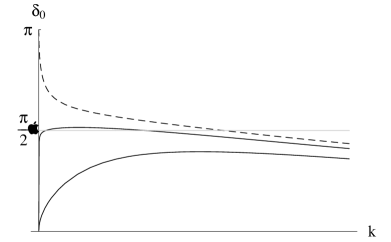
FIG. 4.: The s-wave phase shifts for a Dirac particle in a spherical well. The critical potential $V_{c}=4.20m$. The solid lines represent potentials of strength $V=4.195m$ (middle line) and $V=4m$ (lowest line). The dashed line is a potential well of strength $V=4.3m$ which contains a bound state. ($a=1/m$).

It can be seen that the s-wave phase shift now just increases through $\frac{\pi}{2}$ for values of the potential that are weaker than a critical value $V_{c}$ and thus we have a very weak resonance by our definition above. As will be shown below, the width of this resonance is large compared to that for the p-wave. This is a new result - we would not expect to obtain resonances for s-waves in a spherical potential well.

The p-wave phase shifts are very similar to those obtained for p-waves in the Schrödinger case and are illustrated below.

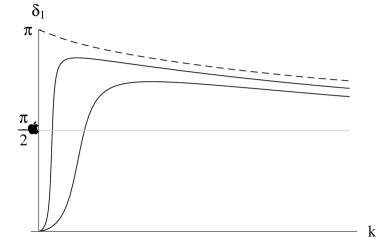
FIG. 5.: The p-wave phase shifts for a Dirac particle in a spherical well. The critical potential $V_{c}=2.30m$. The solid lines represent potentials of strength $V=2m$ (lowest line) and $V=2.2m$ (middle line). The dashed line is a potential well of strength $V=2.4m$ which contains a bound state. ($a=1/m$).

For energies close to the resonant energy position, $E_{R}$, the resonance has the Breit-Wigner form:

$$\tan\delta_{l_{\chi}}\simeq\frac{\Gamma_{l_{\chi}}/2}{E_{R}-E}$$ (72)

where $\Gamma_{l_{\chi}}$ is the width. This width is related to the time delay [11] by

$$\Gamma_{l_{\chi}}\simeq\frac{1}{\tau_{l_{\chi}}}$$ (73)

By taking the ratio of the widths of the s-wave resonance for $V=4.195m$ and the p-wave wave resonance for $V=2.25m$, the s-wave resonance is seen to be approximately $230$ times wider.

For a very clear illustration of the existence of s-wave resonances for the relativistic spherical well, we use the values for the well width $a$ and depth $V$ of Pieper and Greiner [12] in their discussion of superheavy nuclei. In that paper they establish the supercritical values for s states but do not consider scattering phase shifts. Here we choose $a$ to $8$ fm and then the first three critical values at $E=m$ and $E=-m$ for s and p states are easily calculated using Eqs. (59, 60, 64 and 66) and are tabulated below:

s (E=m)	s (E=-m)	p (E=m)	p (E=-m)
75.947	77.997	76.975	79.012
153.434	155.480	154.458	156.498
230.919	232.964	231.942	233.983

Table 1: The critical well depths in MeV for s- and p- states at $E=\pm m$.

The critical well for the $1s_{\frac{1}{2}}$ state is now weakened slightly by 1% to make the depth $V=75.187$ MeV. The phase shift is seen to be:

FIG. 6.: The $1s_{\frac{1}{2}}$ phase shift and energy dependence of $\sin^{2}\delta_{0}$ for the spherical well ($a=8$ fm and $V=75.187$ MeV).

The phase shift is clearly seen to increase through $\frac{\pi}{2}$ corresponding to a resonance. The energy dependence of $\sin^{2}\delta_{0}$ is plotted beside the phase shift and the width is found to be $\Gamma_{0}=41.83$ keV.

Similarly the critical well for the $2p_{\frac{1}{2}}$ state is weakened slightly by 1% to make the depth $V=76.205$ MeV. The phase shift and energy dependence of $\sin^{2}\delta_{1}$ is seen to be:

FIG. 7.: The $2p_{\frac{1}{2}}$ phase shift and energy dependence of $\sin^{2}\delta_{1}$ for the spherical well ($a=8$ fm and $V=76.205$ MeV).

The width of the $2p_{\frac{1}{2}}$ resonance is seen to be $\Gamma_{1}=11.5$ keV. The $2p_{\frac{1}{2}}$ phase shift is seen to increase more rapidly through $\frac{\pi}{2}$ than the $1s_{\frac{1}{2}}$ phase shift and consequently the $1s_{\frac{1}{2}}$ resonance is wider than the $2p_{\frac{1}{2}}$ resonance by a factor of approximately $3.6$.

In order to understand why s-wave resonances occur for relativistic particles we de-couple the large, $f$, and small, $g$, components of Eqs. (14) to form two second order equations. In the case of a general short-range potential the equations for solutions outside the potential are:

$$g^{\prime\prime}-\left[E^{2}-m^{2}-\frac{\chi(\chi+1)}{r^{2}}\right]g(r) = 0$$ (74)

$$f^{\prime\prime}-\left[E^{2}-m^{2}-\frac{\chi(\chi-1)}{r^{2}}\right]f(r) = 0$$ (75)

What happens is that the angular momentum barrier for the large component vanishes for $s_{\frac{1}{2}}$-waves when $\chi=-1$ but the small component still has an angular momentum term. In contrast for $p_{\frac{1}{2}}$-waves ($\chi=1$), the barrier remains for the large component but disappears for the small component so the centrifugal barrier never vanishes for both $f$ and $g$. With this angular momentum term in one or more of the components we are considering cases analogous to the $l>0$ type scattering in the Schrödinger equation and hence this gives rise to real resonances.

Phase Shift Behaviour : The Spherical Barrier

In the case of low momentum scattering $E\to m$ on the spherical barrier, the analysis of the previous section can be repeated with $V\to-V$. The barrier momentum is now $p\to q=\sqrt{(E-V)^{2}-m^{2}}$. In the limit $E\to m$ this becomes $q\to p_{-}$. The corresponding form of Eq. (68) for scattering from barriers is

$$\frac{j_{-\chi-1}(p_{-}a)}{j_{-\chi}(p_{-}a)}=\frac{2ma}{1+2\chi}\sqrt{\frac{V}{V-2m}}$$ (76)

which is the supercritical result for $\chi>0$ given by Eq. (59). Similarly Eq. (69) becomes

$$j_{\chi-1}(p_{-}a)=0$$ (77)

which is the supercritical result for particles with $\chi<0$ given by Eq. (53).

In the previous section we showed that the conditions for s-wave resonance scattering at low momenta off a spherical well agreed with the critical conditions at $E=m$ calculated from the bound s state spectrum of that well. The same is true for p waves. However when s-waves are incident on a barrier this occurs for critical potentials which correspond to the supercritical values for p-waves in the spherical well (i.e. when the p-wave is at $E=-m$). Similarly scattering p-waves are in resonance when the s-wave is supercritical. This phenomenon is known as crossing and was first discussed by two of us [4] in a discussion of positron scattering from heavy nuclei. Under the transformation $E\to-E$, $V\to-V$, $\chi\to-\chi$, $f\to g$, the coupled equations (14) are seen to be invariant. Consequently a supercritical $2p_{\frac{1}{2}}$ state for a well corresponds to a resonant $1s_{\frac{1}{2}}$ state at $E=m$ on a barrier.

In order to calculate the $1s_{\frac{1}{2}}$ phase shift for scattering from a barrier we must use this result to calculate the supercritical condition for $2p_{\frac{1}{2}}$ particles. By strengthening the supercritical well slightly by $1$%, which, through crossing, increases the height of the barrier, the $1s_{\frac{1}{2}}$ phase shift and partial cross-section are seen to be:

FIG. 8.: The $1s_{\frac{1}{2}}$ phase shift and energy dependence of $\sin^{2}\delta_{0}$ for the spherical barrier ($a=8$ fm and $V=79.802$ MeV) .

We see a very clear s-wave resonance with width $\Gamma_{0}=43.1$ keV. Similarly if the supercritical well for the $1s_{\frac{1}{2}}$ state is strengthened by 1% the phase shift for scattering from the barrier $V=78.777$ MeV is:

FIG. 9.: The $2p_{\frac{1}{2}}$ phase shift and energy dependence of $\sin^{2}\delta_{1}$ for the spherical barrier ($a=8$ fm and $V=78.777$ MeV).

The width of the $1s_{\frac{1}{2}}$ resonance is seen to be $\Gamma_{1}=11.8$ keV and the ratio of widths of the $1s_{\frac{1}{2}}$-wave to the $2p_{\frac{1}{2}}$-wave is found to be $3.7$.

General Potentials

The reasoning we have used to understand the analytical results obtained for the spherical well applies equally to monotone short-range potentials with more general shapes that vanish at infinity. We shall suppose that the potential $V(r)$ is spherically symmetric and is given by

$$V(r)=\pm\ vw(r/a)$$ (78)

where $v>0$ is a depth parameter, $a$ is a range parameter, $x=r/a>0$ is a dimensionless distance, and $w(x)$ is a dimensionless shape function. Thus $\ w(x)=e^{-x^{2}}$ represents a Gaussian potential and $w(x)=1,\ x<1;\ w(x)=0,\ x\geq 1$ is the spherical well which we have already studied analytically. Clearly we cannot always expect to find exact analytical solutions. Numerical methods are flexible and powerful but involve arbitrary features, such as iteration method, step size, and boundary at ‘infinity’, which introduce corresponding uncertainties. Our approach is therefore to build a programme, a kind of ‘virtual laboratory’, to test it on the spherical well, and then to apply it to the Gaussian potential. For $V(r)<0,$ this programme would have to be able to find discrete eigenvalues; for potentials of either sign, it would need to be able to compute the wave-function amplitudes at the origin resulting from spherical waves of unit amplitude which are directed towards the origin from far away. Since the scattering process is, in principle, reversible, we shall actually start waves with amplitude $C$ at the origin, and then adjust $C$ so that the waves at distant points have unit amplitude. In addition, we shall need to define and compute a ‘numerical phase (shift)’. This question has been discussed in detail in reference [13].

We shall now explain more fully what we mean in this discussion by the terms ‘amplitude’ and ‘numerical phase’. For very small values of $r,$ the potentials we study are essentially indistinguishable from spherical wells or barriers. Hence the boundary conditions at the origin are the same as those for the exact spherical well solutions (Eq. 16). We shall find it convenient to separate the sign and the magnitude of $\chi$ by use also of the symbols $k=|\chi|=j+\frac{1}{2},$ and $\tau=\chi/|\chi|=\chi/k.$ In the small-$r$ region we may write for $\chi>0$

$$f = Cr^{k+1}$$ (79)

$$g = C^{\prime}r^{k}=\sigma Cr^{k}$$ (80)

$$\frac{rg}{f} = \frac{2k+1}{E+m-V}=\frac{C^{\prime}}{C}=\sigma$$ (81)

$$\sqrt{f^{2}+g^{2}} = |C|r^{k}\sqrt{r^{2}+\sigma^{2}}\approx\sigma|C|r^{k},\quad r\ll 1$$ (82)

and for $\chi<0$

$$f = Cr^{k}$$ (83)

$$g = C^{\prime}r^{k+1}=\sigma Cr^{k+1}$$ (84)

$$\frac{g}{rf} = \frac{V-E+m}{2k+1}=\frac{C^{\prime}}{C}=\sigma$$ (85)

$$\sqrt{f^{2}+g^{2}} = |C|r^{k}\sqrt{1+r^{2}\sigma^{2}}\approx|C|r^{k},\quad r\ll 1.$$ (86)

Ignoring the $fg$-ratio factor $\sigma,$ we shall say of these cases that the amplitude at the origin is $C.$ We therefore seek the value of $C$ which yields $\sqrt{f^{2}+g^{2}}=1$ as $r\rightarrow\infty.$ We recall that the ‘radial functions’ $f(r)=r\psi(r)$ and $g(r)=r\phi(r)$ each have in their definitions a factor $r;$ for bound states we have (omitting the angular factor $4\pi)$ the corresponding normalisations,

$$\int_{0}^{\infty}\sqrt{f^{2}(r)+g^{2}(r)}dr=\int_{0}^{\infty}\sqrt{\psi^{2}(r)+\phi^{2}(r)}r^{2}dr=1.$$ (87)

If we consider the case $j=1/2\Rightarrow k=1,$ then we have for $\chi>0$ $\sqrt{\psi^{2}(0)+\phi^{2}(0)}=\sigma|C|,$ and for $\chi<0$ $\sqrt{\psi^{2}(0)+\phi^{2}(0)}=|C|.$ This example explains our use of the phrase ’amplitude at the origin’ to describe $C.$

At large distances the asymptotic scattering solutions are essentially sinusoidal, like those of the spherical barrier (Eqs. 31,32). In this region, we choose a certain node $\nu$ in $g$, thus $g(r_{\nu})=0,$ and the amplitude $\sqrt{f^{2}+g^{2}}$ at this point is given by $|f(r_{\nu})|.$ Since for the Gaussian potential, the potential value $V(r)$ is never zero, we must choose a sufficiently far node that the ‘sinusoidal’ asymptotic region has essentially been reached. For the spherical well and Gaussian potential we have found $\nu=20$ to be satisfactory. Our task then is to fix $\nu$ and then determine $C$ so that $|f(r_{\nu})|=1.$ Equivalently, we can set $C=1,$ and then use the resulting $|f(r_{\nu})|^{-1}$ as the value of $C$ sought. It may be helpful at this point to see the wave functions in a particular case: they are shown in Figure 10 for the scattering of $s_{\frac{1}{2}}$-state waves of momentum $p=0.1$ by a Gaussian barrier.

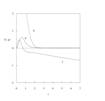
(a) The large ($f$) and small ($g$) components for $r\leq 7$.

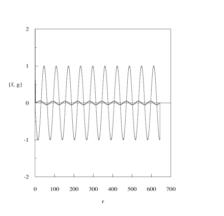
(b) The ‘large component’ $f$ has a maximum of $1$ near the 20th node $r_{20}=635.2$ of the ‘small component’ $g$.

FIG. 10.: Resonant s-wave wave function components for a particle with incident momentum $p=0.1$ scattering from a Gaussian barrier $V(r)=v\,\exp(-r^{2})$, $v=6.8$.

The node $r_{20}$ of $g$ has been detected at $r_{20}=635.2$, and the corresponding maximum of $f$ has the value $1$ with the choice $C=12.8.$ The final determination of the maximum is achieved by fitting a sine function to $f(r)$ locally, as will now be explained.

The position of the maximum allows us at the same time to determine what we shall call the ‘numerical phase’ $\delta.$ We use a modular function to compare the position of the peak with respect to a grid. The details of our function have some arbitrary elements which have been designed to yield a suitably scaled indicator of the phase. We start with an explicit model of the wave function for the large-$r$ asymptotic region. The step size of our numerical integration procedure is represented by $h.$ The $\nu^{\rm th}$ node $r=r_{\nu}$ of $g$ indicates the approximate position of the maximum in $f.$ We write

$$f(r)=\alpha=D\sin(pr+\delta^{\prime}),\quad\beta=f(r+h),\quad\theta=pr+\delta^{\prime}.$$ (88)

Provided $\alpha\neq\beta$ and $\sin(\theta)\neq 0$ (special equations are required for the rare cases of equality), we find

$$\theta=\tan^{-1}\left(\frac{\sin(ph)}{\cos(ph)-\beta/\alpha}\right),\quad D=\frac{\alpha}{\sin(\theta)}.$$ (89)

We now define $\delta$ by the equations

$$\delta_{1}=\theta-pr+(1-\tau)\frac{\pi}{4},\quad\delta=\delta_{1}-\pi\lfloor\delta{{}_{1}}/\pi\rfloor+\frac{\pi}{2},$$ (90)

where we have used $\lfloor x\rfloor$ to represent the integer part of $x$ (often written as ${\rm int}(x)$ in computer languages). This definition of $\delta$ yields a number in the range $\delta\in[-\frac{\pi}{2},\frac{\pi}{2}].$ We have added a plot of $\delta(v)$ to the top of our resonance graphs of $C(v),$ presented below. Eq. (89) also indicates explicitly how $C(v)$ is found: the value of $v$ is chosen; the value of $C$ in Eq. (86) is set to 1; the value of $D$ is determined by Eq. (89); then we have $C(v)=D^{-1}.$ In order to plot Figure 2b, the value of $C$ in Eq. (86) is now set to $C(v)$ just found, and this leads to $D=1,$ as the graph shows. All this computational activity is packaged in the form of a C++ class called ‘dirac’. An instance ‘dc’ of dirac is created and messages are sent to dc to set the potential and the coupling $v$ and the initial conditions etc; dc is then requested to compute eigenvalues and to perform scattering ‘experiments’, and to report the results.

This scattering quantity can be written in a closed form for the spherical potential. We start by looking at the asymptotic form of the wave function for very large values of $r$ given by Eqs. (31 to 36), it is possible to find a value of $r=R$ where the wave function has a peak (or node) in the top component and a corresponding node (or peak peak) in the bottom component. One such set of values is given by

$$R=\frac{1}{k}\left(N\pi+l_{\chi}\frac{\pi}{2}-\delta_{l_{\chi}}\right)$$ (91)

where $N$ is an arbitrarily large integer. From this choice the $f$ component will exhibit a node whilst the $g$ component will be at a peak or trough of the sinusoidal wave. The modulus of the wave function at $r=R$ from Eqs. (31 and 32) is seen to be

$$|\Psi(R)|=\frac{A}{E+m}=\frac{\sqrt{b_{1}^{2}+b_{2}^{2}}}{E+m}$$ (92)

$\rho$ is a measure of the amplitude of the wave function at the origin when the modulus of the incident wave at great distances is unity. It is therefore important to examine the form of the wave function very close to the origin. The components of the wave function inside the potential have the form given by Eqs. (16). Using the following identity for the limiting value of the spherical Bessel function for small arguments

$$\lim_{x\to 0}\left[x^{-n}j_{n}(x)\right]=\frac{1}{(2n+1)!!}$$ (93)

$$\Psi(r)=\left(\begin{array}[]{c}f(r)\\ g(r)\end{array}\right)\to a_{1}\left(\begin{array}[]{c}\frac{r(pr)^{l_{\chi}}}{(2l_{\chi}+1)!!}\\ \frac{\chi}{|\chi|}\frac{1}{E-V+m}\frac{(pr)^{l_{-\chi}+1}}{(2l_{-\chi}+1)!!}\end{array}\right)$$ (94)

The modulus of the wave function at the origin is therefore

$$|\Psi(0)|=\sqrt{f^{2}(0)+g^{2}(0)}\simeq\left\{\begin{array}[]{cl}a_{1}\displaystyle{\frac{p^{\chi}}{E-V+m}}\displaystyle{\frac{1}{(2\chi-1)!!}}r^{\chi}&\qquad\chi>0\\[8.5359pt] a_{1}\displaystyle{\frac{p^{-\chi-1}}{(-2\chi-1)!!}}r^{-\chi}&\qquad\chi<0\end{array}\right.$$ (97)

In particular for s-waves

$$|\Psi(0)|\simeq a_{1}r$$ (98)

whilst for p-waves

$$|\Psi(0)|\simeq a_{1}\frac{pr}{E-V+m}$$ (99)

in agreement with Eqs. (82 and 86). Following the argument given above we can set $a_{1}=1$ and the quantity $C(\pm)$ - where the sign indicates a barrier (+) or well (-) - is found by

$$C(\pm)=\left|\frac{1}{\Psi(R)}\right|$$ (100)

This can be established upon substitution of Eqs. (92, 26 and 27) into the above. $C(-)$ can be established from the above by the transformation $V\to-V$.

For $m=1$ we decided first to study three resonance curves, that is to say, graphs of $C(v)$ for a range of $v>0$ large enough to reach just beyond the third resonance (this is illustrated for the Gaussian potential). We kept $j=\frac{1}{2}$ constant and studied the four cases: $\tau=-1$ ($s_{\frac{1}{2}}$), $\tau=1$ ($p_{\frac{1}{2}}$), repulsive barrier $(+),$ and attractive well $(-).$ For both of the potentials we found that the resonances associated with the attractive wells corresponded exactly to the critical eigenvalues at $E=m$ in the same sector, $s$ or $p;$ whereas, for scattering from barriers, the resonances corresponded, in agreement with our crossing theorem, to the eigenvalues $E=-m$ in the ‘other’ sector, $s$ to $p,$ and $p$ to $s.$ For the spherical potential, the exact critical couplings are given by the following formulas in the $p$–sector:

$$p_{\frac{1}{2}}(-)\quad \Rightarrow \quad v=\left(1+(n\pi)^{2}\right)^{\frac{1}{2}}-1,\quad n=1,2,3,\dots$$ (101)

$$p_{\frac{1}{2}}(+)\quad \Rightarrow \quad v=\left(1+(n\pi)^{2}\right)^{\frac{1}{2}}+1,\quad n=1,2,3,\dots$$ (102)

which can be established from Eqs. (56 and 60) with $a=1$. The corresponding values in the $s$-sector are found as solutions (Eqs. 55 and 62) to a quasi-bound state problem in which the spinor is not normalised since $\phi(r)$ approaches a constant non-zero value as $r\rightarrow\infty.$ The numerical values relevant to the resonance curves are shown in Table 1.

$s_{\frac{1}{2}}(+)$	$s_{\frac{1}{2}}(-)$	$p_{\frac{1}{2}}(+)$	$p_{\frac{1}{2}}(-)$
5.27	1.11	4.30	2.30
8.40	4.20	7.36	5.36
11.54	7.33	10.48	8.48

Table 2: Critical couplings for scattering from spherical barriers $(+)$ and wells $(-)$.

As we have explained, these critical couplings correspond to $(V<0)$ eigenvalues $E=\pm m$ by the rules:

$$s_{\frac{1}{2}}(+) \leftrightarrow (E=-m)p_{\frac{1}{2}},$$ (103)

$$p_{\frac{1}{2}}(+) \leftrightarrow (E=-m)s_{\frac{1}{2}},$$ (104)

$$s_{\frac{1}{2}}(-) \leftrightarrow (E=m)s_{\frac{1}{2}},$$ (105)

$$p_{\frac{1}{2}}(-) \leftrightarrow (E=m)p_{\frac{1}{2}}.$$ (106)

The corresponding $C(p)$ resonance curves are shown in Figure 11.

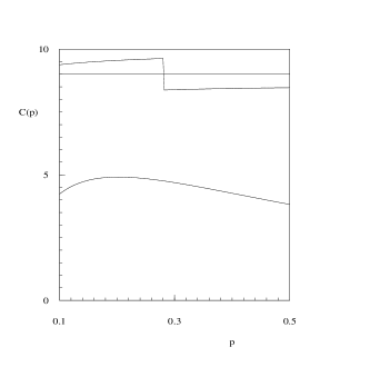
(a) $C(p)$ for s-wave scattering from a spherical barrier of height $U=5.29$.

(b) $C(p)$ for p-wave scattering from a spherical barrier of height $U=4.4$.

(c) $C(p)$ for s-wave scattering from a spherical well of depth $U=-4.195$.

(d) $C(p)$ for p-wave scattering from a spherical well of depth $U=-2.2$.

FIG. 11.: These plots show the scattering measurement $C(p)$ plotted against the incident momentum $p$ for $s$ and $p$ waves incident on supercritical spherical barriers and subcritical wells.

By repeating the analysis for the Gaussian potential, we obtain the resonance peaks and corresponding eigenvalues $E=\pm\ m$ at the critical couplings shown in Table 2.

$s_{\frac{1}{2}}(+)$	$s_{\frac{1}{2}}(-)$	$p_{\frac{1}{2}}(+)$	$p_{\frac{1}{2}}(-)$
6.75	1.26	5.62	2.96
10.42	4.37	9.23	6.11
14.04	7.70	12.83	9.44

Table 3: Critical couplings for Gaussian barriers $(+)$ and wells $(-).$

The resonance curves $C(v)$ for an incident momentum of $p=0.1$ for the Gaussian potential are shown in Figure 12. We have also computed the critical couplings corresponding to $s$ and $p$ states with $E=-m=-1$ and $E=m=1.$ Allowing for $s\leftrightarrow p$ crossing in the $E=-m$ cases, these values agree with the scattering results reported in Table 1. The heights of the peaks in these resonance curves are somewhat arbitrary: they depend on the choice of $p,$ and, more randomly, on the number of $v$ values used in the plot. Ideally we should have $p\rightarrow 0:$ the barrier peaks are sharper for smaller $p,$ and their heights become unbounded; these effects can be ‘seen’ numerically by fine explorations of $C(v)$ for $v$ near critical values. However, as $p$ is reduced, the scale of the relevant part of the wave function expands, and the numerical integration must be carried out to greater and greater distances. The choice $p=0.1$ and its implications are therefore arbitrary. Moreover, the plots we exhibit were made with $n_{v}=400$ points in the abscissae: the closeness to which the resulting values of $v$ lie to critical values is therefore a matter of chance. The resulting numerical maxima have these arbitrary aspects, which, of course, emphasise, by comparison, the great importance of the study of exact analytical solutions when such are available.

(a) s-wave resonances and phase shift for the Gaussian barrier.

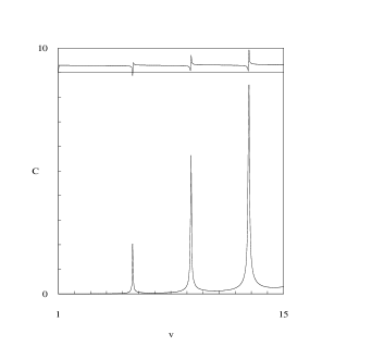
(b) p-wave resonances and phase shift for the Gaussian barrier.

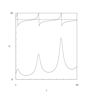
(c) s-wave resonances and phase shift for the Gaussian well.

(d) p-wave resonances and phase shift for the Gaussian well.

FIG. 12.: These plots show the scattering measurement $C(p)$ plotted against the incident momentum $p$ for $s$ and $p$ waves incident on supercritical Gaussian barriers and subcritical wells.

We have found similar results for other short-range potential shapes, such as the exponential potential $w(x)=e^{-x}$ and the Wood-Saxon potential $w(x)=1/(1+e^{x-1}).$

Conclusions

We have reviewed the concept of a resonance in potential scattering in quantum mechanics in terms of the Wigner criterion that not only must the phase shift pass through $\pi/2$ but there must also be a positive time delay in the scattering process. In non-relativistic scattering from a monotone spherically-symmetric potential well that implies that s-wave resonances do not exist, but that p-wave and higher angular momentum resonances do exist. The zero energy solutions of the Schrödinger equation provide a starting point for the study of resonances for scattering off a well: resonances are obtained by slightly weakening the potential needed to obtain a zero energy solution.

In the case of relativistic potential scattering using the Dirac equation, the zero energy solutions are replaced by zero momentum or critical solutions at $E=m$ and $E=-m$. Now resonances are obtained by slightly weakening the critical potential well giving $E=m$ or slightly strengthening the supercritical well giving $E=-m.$ In the case where a critical solution at $E=m$ exists for a potential well, slightly weakening the potential will give rise to resonances in s-waves as well as in higher waves. Slightly increasing the strength of the the supercritical well will give rise to resonances in scattering from a potential barrier using the crossing theorem, which relates positive energy solutions of the Dirac equation for a potential barrier to negative energy solutions for a potential well. We thus find that resonances exist for scattering from barriers in s-waves and higher waves. In particular crossing relates s-wave solutions for a well to p-wave solutions for a barrier and vice versa.

REFERENCES

- [1] Wigner, E. P., Phys. Rev. 98, 145 (1955).
- [2] Newton, R. G., Scattering Theory of Waves and Particles, (Springer-Verlag, Berlin 1982).
- [3] Schiff, L., Quantum Mechanics, (McGraw Hill, New York, 1949).
- [4] Dombey, N. and Hall, R. L., Phys. Lett. B474, 1 (2000).
- [5] Joachain, C. J., Quantum Collision Theory, (North-Holland, Amsterdam, 1983).
- [6] Kamke, D., Am. J. Phys. 53, 274 (1985).
- [7] Greiner, W., Müller, B. and Rafelski, J., Quantum Electrodynamics of Strong Fields, (Springer-Verlag, Berlin, 1985).
- [8] Barthélémy, M-C., Ann. Inst. Henri Poincaré 6, 365 (1967).
- [9] Barthélémy, M-C., Ann. Inst. Henri Poincaré 7, 115 (1967).
- [10] Arfken, G., Mathematical Methods for Physicists, (Academic Press, Inc., 1985).
- [11] Landau, R. H., Quantum Mechanics II: A Second Course in Quantum Theory, (Wiley & Sons, 1996).
- [12] Pieper, W. and Greiner, W., Z. Physik 218, 327 (1969).
- [13] Iwinsky, Z. R., Rosenberg, L. and Spruch, L., Phys. Rev. A31, 1229 (1985).