Kink manifolds in a three-component scalar field theory

Abstract

In this work we identify the manifold of solitary waves arising in a three-component scalar field model using the Bogomol’nyi arrangement of the energy functional. A rich structure of topological and non-topological kinks exists in the different sub-models contained in the theory.

1 Introduction

The search for solitary waves is an ongoing topic in both Mathematics and Physics because this kind of quasi-soliton plays an important r$\hat{{\rm o}}$le in a huge number of branches of non-linear science. In Field Theory, they usually appear in models that support spontaneous symmetry breaking, the most prominent examples being kinks/domain walls, vortices, and monopoles [1]. Starting with theories that involve a high number of fields, the usual procedure followed to investigate the existence of solitary waves -topological defects- is to obtain an effective scalar field theory, imposing severe restrictions on the original theory. In most cases, one is compelled to pursue an effective theory that will correspond to a single scalar field model, where the existence of topological defects can be checked easily. The reason for this is the good-understanding of this kind of system; as paradigmatic examples, the well-known kink and soliton in the one-dimensional $\phi^{4}$ and sine-Gordon models should be noted. Both kinds of solitary wall can be thought of as thick walls, the topological defects in a three-dimensional perspective. Nevertheless, the general framework is that the effective theory depends on several scalar fields and thus the truncation may involve an important loss of information concerning the presence of topological defects and the structure of spontaneous symmetry breaking. It is therefore desirable to investigate the general properties of domain wall solutions in a multi-scalar field theory.

In (1+1)-dimensional field theory, solitary waves are non-singular solutions of the non-linear coupled field equations of finite energy such that their energy density has a spacetime dependence of the form: $\varepsilon(x,t)=\varepsilon(x-vt)$, where $v$ is the velocity of propagation. In relativistic theories, Lorentz (or Galilean) invariance provides all the kink solutions from the purely static ones. The search for finite-energy static solutions in one-dimensional field theories is tantamount to the search for finite action trajectories in a natural dynamical system where, the $x$-coordinate plays the r$\hat{{\rm o}}$le of time; the field components transmute to positions in the configuration space, and the field theoretical density energy becomes minus the mechanical potential energy. No wonder the difficulties involved in finding kinks in multi-component scalar field theories: one faces multi-dimensional mechanical systems where integrability is not ensured.

At a very early stage in the (pre-)history of the subject, a (1+1)-dimensional field theoretical model with two real scalar fields became relevant. Montonen and Sarker-Trullinger-Bishop proposed the deformation of the $O(2)$-linear sigma model with a potential energy density of $U(\phi_{1},\phi_{2})={1\over 2}[(\phi_{1}^{2}+\phi_{2}^{2}-1)^{2}+\sigma^{2}\phi_{2}^{2}]$, see [2]. It was clear that the zeroes of the potential are two points and hence the hunt for kinks started immediately. Using a trial orbit method in the associated two-dimensional mechanical system, Rajaraman identified two different topological kinks joining the two vacua of the system that live on a straight line and half-ellipses respectively. Only one component of the scalar field is non-zero in the first case, but the two-components differ from zero in the second kind of solution; for this reason, these solitary waves are referred to as TK1 (straight line) and TK2/TK2* (upper/lower half-ellipse) kinks in the literature that appeared later. Rajaraman also found one kink associated to a closed trajectory starting from and ending at the same point of the the vacuum orbit. Magyari and Thomas [3] realized that the mechanical system associated with the MSTB model is integrable -there is a second invariant in involution with the mechanical energy- and used this fact to show that there exists a whole family of two-component non-topological kinks (NTK2), all of them degenerated in energy with Rajaraman’s NTK2 kink; explicit kink form factors were only described by numerical methods.

The main breakthrough in analytically finding all the solitary waves of the MSTB model emerged in Reference [4]. Ito discovered that the mechanical problem was not only integrable but that it was Hamilton-Jacobi separable by using elliptic coordinates. In this setting, he showed the analytic formulas for the kink orbits and the kink form factors, unveiling the mathematical reasons for the previously observed striking kink sum rule. Immediately, the stability of this degenerate kink family was questioned; application of the Morse index theorem solved this problem in [5]. A parallel with the Morse theory of geodesics was established somewhat later in Reference [6]. Thus, a clear connection arose between solitary waves, their stability, and dynamical systems. In Reference [7], several of us showed that the MSTB model is not unique in this respect; two (1+1)-dimensional field theoretical models with two real scalar fields -referred to as model A and B in that paper- have manifolds of solitary waves with similar structures. To find the analytic expression for the kinks of model A, we were prompted to solve an integrable dynamical system classified as Liouville Type I, see [8]. The system belongs to the same class as that found in the MSTB model -the two-dimensional Garnier system [9]- but there are three differences: (a) the potential energy density is a polynomial of sixth order in the fields (instead of fourth); (b) the vacuum orbit has five points (instead of 2), and (c) there are many more stable kinks than in the MSTB model. Model B is characterized by a fourth-order potential energy density in the two scalar fields. The main feature, however, is the need to solve a Liouville integrable system of Type III, i.e. Hamilton-Jacobi separable in parabolic coordinates. The vacuum orbit has four points and there are manifolds of stable and unstable kinks.

In recent years, all this work has proved to be fruitful in the framework of supersymmetric theories. In the dimensional reduction of a generalized Wess-Zumino model with two chiral superfields, Bazeia-Nascimento-Ribeiro-Toledo (henceforth referred to as the BNRT model) [10] found one one-component topological kink (TK1) and one two-component topological kink (TK2). In this case, the vacuum orbit has four points and the potential energy density is a polynomial in the fields of order four. Understanding the BNRT model as a deformation of model B, some of us discovered the whole manifold of kink orbits [11]. There is kink degeneracy, also found slightly earlier by Shifman and Voloshin in one of the topological sectors [12], and, for two critical values of the coupling constant, analytic formulas for the kink form factors are available. One of them corresponds exactly to model B; the other one leads to a Liouville system of Type IV, Hamilton-Jacobi separable in Cartesian coordinates. Interesting consequences have been translated to the dynamics of intersecting branes [13]. How thick walls grow from one-component kinks is well known. Composite kinks give rise to a non-trivial low energy dynamics for intersecting walls as geodesic motion in the kink moduli space (the space of the integration constants with a metric inherited from the field theoretic kinetic energy). Another supersymmetric model that shows a rich pattern of kink solutions is the Wess-Zumino model itself. The BPS kink states of this ${\cal N}=2$ supersymmetric $(1+1)D$ model with a complex scalar field and holomorphic superpotential were discovered by Vafa et al. in [14]. In [15], two of us studied this system from the point of view of the real-analytic structure. The vacuum orbit having been identified, the flow between the vacuum points was determined as the gradient of the real(imaginary) part of the superpotential. Thus, kink orbits are identified with real algebraic curves.

Here, we continue to struggle with the extension of these studies to field theoretical models with three real scalar fields. In [16], some of us explored the generalization of the MSTB model. The solution of the three-dimensional Garnier system using three-dimensional Jacobi coordinates revealed the existence of an extremely complex variety of kinks. Nevertheless, the structure of the kink manifold and its stability was completely unraveled in [17]. The main goal of the present paper is to identify the kink manifold arising in a family of three-component relativistic field models with a vacuum manifold that contains several elements or points. This family can be interpreted as the natural generalization of the generalized MSTB model studied in [16][17] in the sense of Stäckel-type systems. The most interesting feature of this generalization is that the number of elements in the vacuum manifold depends on the range of relative values of the coupling constants. Therefore, we can find different submodels of our system, which have a very rich structure of kink manifolds. When the energy density of these kinks or solitary waves is studied we find that several families of these solutions are degenerate, which allows us to claim that some kink families indeed consist of more basic kinks, such that their energy density displays several lumps associated with the basic kinks. In our model, we are able to find solutions with two, three or four lumps.

The organization of the paper is as follows: In Section 2 we introduce the model, writing the expressions in Stäckel form and describing the different spontaneous symmetry-breaking scenarios. Section 3 is divided into four sub-sections. In 3.1, we identify first-order differential equations satisfied by the kink solutions, reproducing the Bogomol’nyi procedure in this context. Sub-section 3.2 contains the resolution of these equations. In 3.3, we determine the regions where the solutions live and, finally, in Sub-section 3.4, some general comments about the determination of the stability of the kink solutions are offered. In Section 4 we describe the behaviour of solitary wave families in one of the regimes of the model, at the same time discussing their stability properties. Finally, in Section 5 we address some points concerning the different extensions of the model.

2 The model

We focus our attention on the search for kink solutions arising in three-component scalar field models in a (1+1) Minkowskian space-time, whose dynamics is governed by the action functional

$$S[\phi]=\int d^{2}x\left[\frac{1}{2}\sum_{j=1}^{3}\partial_{\mu}\phi_{j}\partial^{\mu}\phi_{j}-U(\phi)\right]\quad,$$

where we use Einstein’s convention for Greek indices with the usual metric $\eta_{11}=-\eta_{22}=1$, $\eta_{12}=\eta_{21}=0$, and where $U(\phi)$ is a smooth non-negative function that depends on the three-component scalar field $\phi=(\phi_{1},\phi_{2},\phi_{3})$. We use natural units, hence $c=1$, and we shall henceforth denote $x^{0}\equiv t$ and $x^{1}\equiv x$. The Euler-Lagrange equations in this case are written as the following system of second-order partial differential equations

$$\frac{\partial^{2}\phi_{i}}{\partial t^{2}}-\frac{\partial^{2}\phi_{i}}{\partial x^{2}}=-\frac{\partial U}{\partial\phi_{i}}(\phi_{1},\phi_{2},\phi_{3})\hskip 14.22636pti=1,2,3\,.$$ (1)

Kinks are finite-energy solutions of (1), such that the time dependence is dictated by the Lorentz invariance: $\phi_{K}(t,x)=\phi(\frac{x-vt}{\sqrt{1-v^{2}}})$, and they can be interpreted as extremals of the positive semi-definite energy functional

$${\cal E}[\phi]=\int dx\,\varepsilon(x)=\int dx\left\{\frac{1}{2}\sum_{i=1}^{3}\frac{\partial\phi_{i}}{\partial x}\frac{\partial\phi_{i}}{\partial x}+U(\phi_{1},\phi_{2},\phi_{3})\right\}\quad,$$ (2)

which maintains this functional finite: ${\cal E}[\phi]<+\infty$, see [1]. Therefore, solitary waves must comply with the asymptotic conditions

$$a)\hskip 14.22636pt\lim_{x\to\pm\infty}\phi\in{\cal M}\hskip 56.9055ptb)\hskip 14.22636pt\lim_{x\to\pm\infty}\frac{d\phi}{dx}=0\quad,$$ (3)

where ${\cal M}$ is the set of zeroes or absolute minima of the potential term -that is, ${\cal M}=\{(\phi_{1},\phi_{2},\phi_{3})\in{\mathbb{R}}^{3}/U(\phi_{1},\phi_{2},\phi_{3})=0\}$- which are usually referred to as vacua of the theory because the elements of ${\cal M}$ play this r$\hat{\rm o}$le in the corresponding quantum theory.

The usual procedure for tackling the search for kinks in this kind of theory is to interpret (2) as the action functional of a mechanical system in which we think of the variable $x$ as “time”; $\phi$ as the coordinates of a unit-mass point particle, and $V=-U$ as the potential function. From this point of view, (1) are merely equations of motion in the new system. In reference [16], the authors deal with the model involving the potential function

$$U(\phi_{1},\phi_{2},\phi_{3})=\frac{1}{2}(\phi_{1}^{2}+\phi_{2}^{2}+\phi_{3}^{2}-1)^{2}+\frac{1}{2}\sigma_{2}^{2}\phi_{2}^{2}+\frac{1}{2}\sigma_{3}^{2}\phi_{3}^{2}$$ (4)

and show that the mechanical analogue is not only completely integrable but also Hamilton-Jacobi separable by using a system of three-dimensional elliptic coordinates. In [17], the stability properties of kinks are analyzed and a new approach to search for kinks based on the Bogomol’nyi decomposition are given in the above system. The authors prove the equivalence between the Hamilton-Jacobi equation and the Bogomol’nyi approach. The potential function (4) has two zeroes, $v^{-}=(-1,0,0),\,v^{+}=(1,0,0)$. Therefore, the kinks in this model can be classified into topological and non-topological kinks according to whether the solution connects two different vacua (open orbits) or the solution departs and arrives at a vacuum (closed orbits).

The search for new integrable models is not an easy task. In this sense, we would remark the following quotation from Jacobi in his “Vorlesungen über Dynamik”, which allows us to see the issue from a different perspective: “The main difficulty in integrating given differential equations is to introduce suitable variables which cannot be found by a general rule. Therefore, we must go in the opposite direction and, after finding some remarkable substitution, look for problems to which it could be successfully applied”.

The goal of this paper is to generalize the above model, focusing our attention on models with a greater-than-two number of elements in ${\cal M}$, such that we can find a more sophisticated symmetry-breaking scenario and a richer plethora of solitary waves than before.

Using the same notation as in the reference [16], we now introduce a system of Jacobi elliptic coordinates ${\bf\lambda}=(\lambda_{1},\lambda_{2},\lambda_{3})$, with constants $\bar{\sigma}_{3}^{2}=1-\sigma_{3}^{2}$, $\bar{\sigma}_{2}^{2}=1-\sigma_{2}^{2}$ and $1$, which is defined as:

$$\phi_{1}^{2} = \frac{1}{\sigma_{2}^{2}\sigma_{3}^{2}}(1-\lambda_{1})(1-\lambda_{2})(1-\lambda_{3})$$

$$\phi_{2}^{2} = \frac{-1}{\sigma_{2}^{2}(\sigma_{3}^{2}-\sigma_{2}^{2})}(\bar{\sigma}_{2}^{2}-\lambda_{1})(\bar{\sigma}_{2}^{2}-\lambda_{2})(\bar{\sigma}_{2}^{2}-\lambda_{3})$$ (5)

$$\phi_{3}^{2} = \frac{-1}{\sigma_{3}^{2}(\sigma_{2}^{2}-\sigma_{3}^{2})}(\bar{\sigma}_{3}^{2}-\lambda_{1})(\bar{\sigma}_{3}^{2}-\lambda_{2})(\bar{\sigma}_{3}^{2}-\lambda_{3})\,,$$

in which the range of the coordinates is:

$$-\infty<\lambda_{1}<\bar{\sigma}_{3}^{2}<\lambda_{2}<\bar{\sigma}_{2}^{2}<\lambda_{3}<1\ .$$ (6)

It should be noted that this coordinate transformation is invariant under the group $G=\mathbb{Z}_{2}^{\times 3}$ generated by $\phi_{a}\to(-1)^{\delta_{ab}}\phi_{a};\,b=1,2,3$.

Invoking (5), the energy functional can be written as

$${\cal E}[\phi]=\int dx\left\{\frac{1}{2}\sum_{j=1}^{3}g_{jj}(\lambda)\frac{\partial\lambda_{j}}{\partial x}\frac{\partial\lambda_{j}}{\partial x}+U(\lambda_{1},\lambda_{2},\lambda_{3})\right\}\ ,$$ (7)

where the metric coefficients $g_{jj}(\lambda)=-\frac{1}{4}\frac{f_{j}(\lambda)}{(\lambda_{j}-1)(\lambda_{j}-\bar{\sigma}_{2}^{2})(\lambda_{j}-\bar{\sigma}_{3}^{2})}$ have been introduced. Here, we set $\displaystyle f_{j}(\lambda)=\prod_{k=1,k\neq j}^{3}(\lambda_{j}-\lambda_{k})$.

In the new variables, the potential (4) is written as:

$$U(\lambda)=\frac{1}{2}\sum_{i=1}^{3}\frac{\lambda_{i}^{2}(\lambda_{i}-\overline{\sigma}_{2}^{2})(\lambda_{i}-\overline{\sigma}_{3}^{2})}{f_{i}(\lambda)}\ ,$$ (8)

and their zeroes $v^{-}$ y $v^{+}$ are mapped to one point $v\equiv(\lambda_{1}^{v},\lambda_{2}^{v},\lambda_{3}^{v})=(0,\bar{\sigma}_{3}^{2},\bar{\sigma}_{2}^{2})$ in the elliptic space because of the above-mentioned invariance.

In order to generalize expression (8), we introduce the following potential function

$$U(\lambda;\bar{\alpha}^{2})=\sum_{i=1}^{3}U_{i}(\lambda;\bar{\alpha}^{2})=\frac{1}{2}\sum_{i=1}^{3}\frac{\lambda_{i}^{2}(\lambda_{i}-\overline{\sigma}_{2}^{2})(\lambda_{i}-\overline{\sigma}_{3}^{2})(\lambda_{i}-\bar{\alpha}^{2})^{2}}{f_{i}(\lambda)}\ ,$$ (9)

which becomes a polynomial function of eighth degree in the original fields. Notice that we have added a new factor $(\lambda_{i}-\bar{\alpha}^{2})^{2}$ to each of the summands in (8). Thus, (9) introduces new degenerate vacua in ${\cal M}$, which for fixed $\overline{\sigma}_{2}^{2}$ and $\overline{\sigma}_{3}^{2}$ depend upon the value of the coupling constant $\bar{\alpha}^{2}=1-\alpha^{2}$. Therefore, new scenarios of spontaneous symmetry-breaking and a richer kink manifold arise in this model. Taking into account the range (6) for the elliptic coordinates and formula (9), we can observe that the new structure of the set ${\cal M}$ depends on the relative values between the constant $\bar{\alpha}^{2}$ and the fixed constants $\bar{\sigma}_{2}^{2}$, $\bar{\sigma}_{3}^{2}$ and $1$. For instance, for $\bar{\alpha}^{2}>1$ the new factor $(\lambda_{i}-\bar{\alpha}^{2})^{2}$ does not vanish for any value of $\lambda_{i}$ and therefore ${\cal M}$ has the same structure as that in model (8). However, for $\bar{\alpha}^{2}\in(\bar{\sigma}_{3}^{2},\bar{\sigma}_{2}^{2})$ we find new vacua located at the points $\lambda\equiv(\bar{\sigma}_{3}^{2},\bar{\alpha}^{2},\bar{\sigma}_{2}^{2})$ and $\lambda\equiv(0,\bar{\alpha}^{2},\bar{\sigma}_{2}^{2})$.

We shall now introduce different scenarios for our model depending on the value of the constant $\bar{\alpha}^{2}$. We shall distinguish the number of vacua in each case.

• Regime $E1$: As mentioned above, for $\bar{\alpha}^{2}\in\left(1,\infty\right)$ there exists only one vacuum in the elliptic space, minimizing the potential function: $\lambda^{v_{1}}=(0,\bar{\sigma_{3}}^{2},\bar{\sigma_{2}}^{2})$. We have a similar situation if the constant $\bar{\alpha}^{2}$ takes the discrete values $0$, $\overline{\sigma}_{3}^{2}$ or $\overline{\sigma}_{2}^{2}$. For this reason we define the set $L_{0}=\left\{0,\overline{\sigma}_{3}^{2},\overline{\sigma}_{2}^{2}\right\}\cup\left(1,\infty\right)$, taking into account that if $\bar{\alpha}^{2}\in L_{0}$ our model only has a vacuum, $\lambda^{v_{1}}$, in the elliptic space. In the Cartesian space, the vacuum manifold ${\cal M}$ can be regarded as the orbit generated by the action of the group $G/H_{1}$ over the vacuum $v_{1}$, where $H_{1}=\mathbf{1}\times\mathbb{Z}_{2}\times\mathbb{Z}_{2}$ is the group that leaves the coordinates of $v_{1}$ invariant. There are therefore two vacua in the Cartesian space ${\cal M}_{0}=\{\phi^{v^{1}}=(\pm 1,0,0)$}.

  The kink solutions in this model display the same behaviour as those of the model studied in [16], although the explicit expression of the equations of motion is more complicated because we have a polynomial of degree eight in the original fields. Owing to this similarity, we shall not deal with this regime in our study.

• Regime $E2$: We now consider the range $\bar{\alpha}^{2}\in L_{1}=\left(0,\overline{\sigma}_{3}^{2}\right)$ for the coupling constant. In this regime, new zeroes of the potential arise on the plane $\lambda_{1}=\bar{\alpha}^{2}$, in the elliptic space that corresponds to the ellipsoid $\frac{\phi_{1}^{2}}{1-\bar{\alpha}^{2}}+\frac{\phi_{2}^{2}}{\bar{\sigma}_{2}^{2}-\bar{\alpha}^{2}}+\frac{\phi_{3}^{2}}{\bar{\sigma}_{3}^{2}-\bar{\alpha}^{2}}=1$ in the Cartesian space. In fact, two vacua arise in the elliptic space, $\lambda^{v^{1}}=(0,\bar{\sigma_{3}}^{2},\bar{\sigma_{2}}^{2})$ and $\lambda^{v^{2}}=(\bar{\alpha}^{2},\bar{\sigma_{3}}^{2},\bar{\sigma_{2}}^{2})$, both invariant under the subgroup $H_{2}=H_{1}$. Correspondingly, there are four vacua in the Cartesian space that correspond to the orbit $\bigsqcup_{i=1}^{2}(G/H_{i})v_{i}$. Therefore, we have ${\cal M}_{1}=\{\phi^{v_{1}}=(\pm 1,0,0),\phi^{v_{2}}=(\pm\alpha,0,0)$}, as depicted in Figure 1.

  It is interesting to remark that the range of values $\bar{\alpha}^{2}\in(-\infty,0)$ is formally analogous to that in which $\bar{\alpha}^{2}\in L_{1}$, interchanging the r$\hat{\rm o}$les of the ellipsoids $\lambda_{1}=0$ and $\lambda_{1}=\bar{\alpha}^{2}$ in the previous reasoning. We shall therefore focus our attention on the range of values $L_{1}$.

  

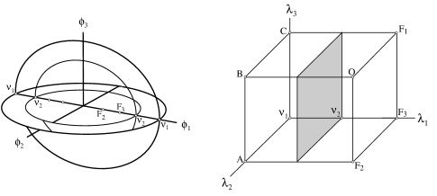
  Figure 1: Vacuum manifold in the Cartesian and elliptic spaces: Regime $E2$. F₁, F₂ and F₃ stand for the foci of the ellipsoid; B and C are the extremes of the minor semi-axis, and A represents the umbilical points.

• Regime $H1$: In this case, $\bar{\alpha}^{2}\in L_{2}=\left(\overline{\sigma}_{3}^{2},\overline{\sigma}_{2}^{2}\right)$. From the values of $\bar{\alpha}^{2}$ and the range of the elliptic coordinates, the zeroes of the potential term (9) arise on the plane $\lambda_{2}=\bar{\alpha}^{2}$, which is equivalent to the hyperboloid of one sheet $\frac{\phi_{1}^{2}}{1-\bar{\alpha}^{2}}+\frac{\phi_{2}^{2}}{\bar{\sigma}_{2}^{2}-\bar{\alpha}^{2}}=1+\frac{\phi_{3}^{2}}{\bar{\alpha}^{2}-\bar{\sigma}_{3}^{2}}$ in the Cartesian space. We find three vacua located at the points $\lambda^{v^{1}}=(0,\bar{\sigma}_{3}^{2},\bar{\sigma}_{2}^{2})$, $\lambda^{v^{2}}=(\bar{\sigma}_{3}^{2},\bar{\alpha}^{2},\bar{\sigma}_{2}^{2})$ and $\lambda^{v^{3}}=(0,\bar{\alpha}^{2},\bar{\sigma}_{2}^{2})$. The vacua $v_{1}$ and $v_{2}$ remain invariant under $H_{1}$, whereas $v_{3}$ is invariant under $H_{3}=\mathbf{1}\times\mathbb{Z}_{2}\times\mathbf{1}$. There are eight vacua in the Cartesian space corresponding to the orbit $\bigsqcup_{i=1}^{3}(G/H_{i})v_{i}$, with coordinates ${\cal M}_{2}=\{\phi^{v_{1}}=(\pm 1,0,0),\phi^{v_{2}}=(\pm\alpha,0,0),\phi^{v_{3}}=(\pm\frac{\alpha}{\sigma_{3}},0,\pm\frac{\bar{\sigma}_{3}}{\sigma_{3}}\sqrt{\bar{\alpha}^{2}-\bar{\sigma}_{3}^{2}})\}$, as shown in Figure 2. In section 4, for the sake of clarity we shall focus on this regime in order to describe in detail a particular kink manifold of the model instead of discussing it in each single regime.

  

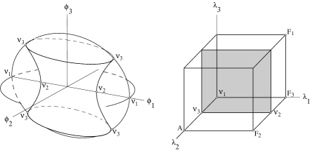
  Figure 2: Vacuum manifold in the Cartesian and elliptic spaces: Regime $H1$.

• Regime $H2$: This case is characterized by $\bar{\alpha}^{2}\in L_{3}=\left(\overline{\sigma}_{2}^{2},1\right)$. Applying the same reasoning as before, we find that new vacua arise on the plane $\lambda_{3}=\bar{\alpha}^{2}$; that is, the hyperboloid of two sheets $\frac{\phi_{1}^{2}}{1-\bar{\alpha}^{2}}=1+\frac{\phi_{2}^{2}}{\bar{\alpha}^{2}-\bar{\sigma}_{2}^{2}}+\frac{\phi_{3}^{2}}{\bar{\alpha}^{2}-\bar{\sigma}_{3}^{2}}$ in Cartesian coordinates. In particular, the potential has four minima: $\lambda^{v_{1}}=(0,\bar{\sigma}_{3}^{2},\bar{\sigma}_{2}^{2})$; $\lambda^{v_{2}}=(\bar{\sigma}_{3}^{2},\bar{\sigma}_{2}^{2},\bar{\alpha}^{2})$; $\lambda^{v_{3}}=(0,\bar{\sigma}_{2}^{2},\bar{\alpha}^{2})$, and $\lambda^{v_{4}}=(0,\bar{\sigma}_{3}^{2},\bar{\alpha}^{2})$. The vacuum $v_{4}$ is invariant under $H_{4}=\mathbf{1}\times\mathbf{1}\times\mathbb{Z}_{2}$, and the Cartesian vacuum manifold is the orbit $\bigsqcup_{i=1}^{4}(G/H_{i})v_{i}$; namely,

  $${\cal M}_{3} = \left\{\phi^{v_{1}}=(\pm 1,0,0),\phi^{v_{2}}=(\pm\alpha,0,0),\right.$$

  $$\left.\phi^{v_{3}}=\left(\pm\frac{\alpha}{\sigma_{3}},0,\pm\frac{\bar{\sigma}_{3}}{\sigma_{3}}\sqrt{\bar{\alpha}^{2}-\bar{\sigma}_{3}^{2}}\right),\phi^{v_{4}}=\left(\pm\frac{\alpha}{\sigma_{2}},\pm\frac{\bar{\sigma}_{2}}{\sigma_{2}}\sqrt{\bar{\alpha}^{2}-\bar{\sigma}_{2}^{2}},0\right)\right\}.$$

  

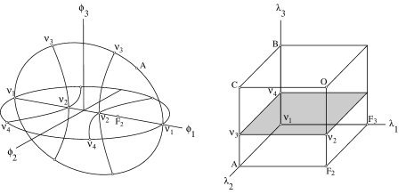
  Figure 3: Vacuum manifold in the Cartesian and elliptic spaces: Regime $H2$.

• Regime $H2\,^{\prime}$: In this case, the coupling constant $\bar{\alpha}^{2}$ is set equal to unity. In the internal elliptic space we can read the minima as $\lambda^{v_{1}}=(0,\bar{\sigma}_{3}^{2},\bar{\sigma}_{2}^{2})$, $\lambda^{v_{2}}=(\bar{\sigma}_{3}^{2},\bar{\sigma}_{2}^{2},1)$, $\lambda^{v_{3}}=(0,\bar{\sigma}_{2}^{2},1)$ and $\lambda^{v_{4}}=(0,\bar{\sigma}_{3}^{2},1)$, which correspond to eight minima in the Cartesian space: ${\cal M}_{3}^{\,{}^{\prime}}=\displaystyle\lim_{\bar{\alpha}^{2}\to 1}{\cal M}_{3}=\{\phi^{v_{1}}=(\pm 1,0,0),\phi^{v_{2}}=(0,0,0),\phi^{v_{3}}=(0,0,\pm\bar{\sigma}_{3}),\phi^{v_{4}}=(0,\pm\bar{\sigma}_{2},0)\}$.

  In this latter case, the plane $\lambda_{3}=1$ is introduced into the elliptic space. Unlike the previously introduced planes, this is no longer a regular one, and this can be readily seen in the degeneracy exhibited by the $H$2 vacuum manifold at the limit $\bar{\alpha}^{2}\to 1$; this singular plane corresponds to the plane $\phi_{1}=0$ in Cartesian coordinates. Regarding the kink manifold, this is basically the same as that of the $H$2 model, except that the kink solutions existing on the two sheets of the hyperboloid and in between them now degenerate into kink solutions on the plane $\phi_{1}=0$. This situation is the 3D analogue of model A in [7].

3 First-order equations and Kink Manifolds

3.1 The superpotential and the Bogomol’nyi arrangement

We notice that the potential (9) determines a Stäckel system [8]. Therefore, the Hamilton-Jacobi equation of the mechanical analogue is separable using the system of Jacobi elliptic coordinates. However, here we shall make use of the Bogomol’nyi arrangement in order to obtain the kink manifold of our model. The two procedures are equivalent (see [17]) but the second one allows us to identify the supersymmetric extension of our field theory, given that if the energy functional (7) can be written as

$${\cal E}[\phi]=\int dx\frac{1}{2}\sum_{j=1}^{3}g_{jj}\left(\frac{\partial\lambda_{j}}{\partial x}\pm\frac{1}{g_{jj}}\frac{\partial W(\lambda)}{\partial\lambda_{j}}\right)^{2}\mp\int dx\frac{dW(\lambda)}{dx}$$ (10)

for some function $W(\lambda_{i})$, then the underlying field theory has a supersymmetric extension in which the function $W$ plays the r$\hat{\rm o}$le of superpotential in the supersymmetric field theory, see [18]. Therefore, the superpotential $W$ must comply with

$$2U(\lambda)=g_{11}^{-1}(\lambda)\left(\frac{\partial W}{\partial\lambda_{1}}\right)^{2}+g_{22}^{-1}(\lambda)\left(\frac{\partial W}{\partial\lambda_{2}}\right)^{2}+g_{33}^{-1}(\lambda)\left(\frac{\partial W}{\partial\lambda_{3}}\right)^{2}\ .$$

Plugging the expression of the potential function (9) and the metric coefficients into the above equation, we have

$$\sum_{i=1}^{3}\frac{\lambda_{i}^{2}(\lambda_{i}-\bar{\alpha}^{2})^{2}\prod_{j=2}^{3}(\lambda_{i}-\overline{\sigma}_{j}^{2})}{f_{i}(\lambda)}=\sum_{i=1}^{3}\frac{-4(\lambda_{i}-1)\prod_{j=2}^{3}(\lambda_{i}-\overline{\sigma}_{j}^{2})}{f_{i}(\lambda)}\left(\frac{\partial W}{\partial\lambda_{i}}\right)^{2}\ ,$$

which can be solved easily by the ansatz $W=W_{1}(\lambda_{1})+W_{2}(\lambda_{2})+W_{3}(\lambda_{3})$. The three resulting decoupled ordinary differential equations

$$\left(\frac{dW_{i}}{d\lambda_{i}}\right)^{2}=\frac{\lambda_{i}^{2}(\lambda_{i}-\bar{\alpha}^{2})^{2}}{4(1-\lambda_{i})}\quad,\quad i=1,2,3$$

lead us to the expression of the superpotential function $W$

$$W^{(\beta_{1},\beta_{2},\beta_{3})}(\lambda)=\sum_{i=1}^{3}W^{\beta_{i}}_{i}(\lambda_{i})=\frac{1}{15}\sum_{i=1}^{3}(-1)^{\beta_{i}}P_{2}(\lambda_{i})\sqrt{1-\lambda_{i}}\ \quad,\quad\beta_{i}=0,1\ ,$$

where $P_{2}(\lambda_{i})=2d+d\lambda_{i}-3\lambda_{i}^{2}$, with $d=(5\bar{\alpha}^{2}-4)$.

Extremal trajectories for the energy functional (10) arise if the following system of first-order differential equations

$$\frac{d\lambda_{i}}{dx} = (-1)^{\beta_{i}}g_{ii}^{-1}(\lambda)\frac{dW_{i}}{d\lambda_{i}}$$ (11)

$$= (-1)^{\beta_{i}}2\frac{\lambda_{i}(\lambda_{i}-\bar{\alpha}^{2})(\lambda_{i}-\overline{\sigma}_{2}^{2})(\lambda_{i}-\overline{\sigma}_{3}^{2})}{f_{i}(\lambda)}\sqrt{1-\lambda_{i}}$$

where $\beta_{i}=0,1$ and $i=1,2,3$ is satisfied, because the squared terms in (10) are always positive and the last one is a constant. Due to the indeterminacy of the signs $\beta_{1}$, $\beta_{2}$ and $\beta_{3}$, (11) constitutes eight systems of ordinary differential equations. Nevertheless, this set of systems is easier to solve than second-order (Euler-Lagrange) equations. In order to obtain a complete kink solution we have to join solutions from the first-order differential equations with different choices of the signs $(-1)^{\beta_{i}}$ in different intervals covering the real line. The reason for this is that the first-order differential equations inherit the information of the second-order equations defined piecewise. Assuming that we search for continuous and differentiable solutions, the sequence of signs $(-1)^{\beta_{i}}$ corresponding to the different pieces that constitutes a solution is prescribed. In section 4 we shall illustrate this approach in several cases. From (10) it is readily seen that the energy of a solitary wave, solution of (11) with only one piece, depends only on the topological charge of the solution. In this case, it is said that the Bogomol’nyi bound is saturated. However, if the orbit $\lambda$ is given by $\lambda=\cup_{j=1}^{J}\lambda^{j}$, where $J$ is the number of pieces of $\lambda$ and $\lambda^{j}$ stands for the $j^{\rm th}$ piece, we have:

$${\cal E}[\lambda] = \sum_{\mbox{\footnotesize pieces of }\lambda}\int dx\frac{dW(\lambda)}{dx}=\sum_{j}\int\sum_{i=1}^{3}\frac{\partial W^{\{\beta_{i}\}_{j}}}{\partial\lambda_{i}}\,d\lambda_{i}$$ (12)

$$= \sum_{j}^{J}(W^{\{\beta_{i}\}_{j}}(\lambda^{j}_{\mbox{\footnotesize final}})-W^{\{\beta_{i}\}_{j}}(\lambda^{j}_{\mbox{\footnotesize initial}}))\ ,$$

where $\{\beta_{i}\}_{j}$ represents the values of the $\beta_{i}$ parameters for the $j^{\rm th}$ piece of the solution.

3.2 Solutions via quadratures

In order to solve system (11), we rewrite it in the form:

$$\frac{d\lambda_{i}}{(-1)^{\beta_{i}}2\sqrt{1-\lambda_{i}}\prod_{j=1}^{4}(\lambda_{i}-c_{j})}=\frac{dx}{f_{i}(\lambda)}\quad,\quad i=1,2,3\ ,$$ (13)

where we have defined $c=(\bar{\alpha}^{2},\bar{\sigma}_{2}^{2},\bar{\sigma}_{3}^{2},\bar{\sigma}_{4}^{2})$ and $\bar{\sigma}_{4}^{2}=0$ for future convenience. The sum of these equations gives

$$\sum_{i=1}^{3}\frac{d\lambda_{i}}{(-1)^{\beta_{i}}2\sqrt{1-\lambda_{i}}\prod_{j=1}^{4}(\lambda_{i}-c_{j})}=0$$ (14)

Multiplying each side of (13) by $\lambda_{i}$ and summing over $i$, we obtain:

$$\sum_{i=1}^{3}\frac{\lambda_{i}d\lambda_{i}}{(-1)^{\beta_{i}}2\sqrt{1-\lambda_{i}}\prod_{j=1}^{4}(\lambda_{i}-c_{j})}=0\ .$$ (15)

Also, multiplying (13) by $\lambda_{i}^{2}$ and summing again over $i$ we reach the equation that establishes the dependence of the kink components on $x$

$$\sum_{i=1}^{3}\frac{\lambda_{i}^{2}d\lambda_{i}}{(-1)^{\beta_{i}}2\sqrt{1-\lambda_{i}}\prod_{j=1}^{4}(\lambda_{i}-c_{j})}=dx\ .$$ (16)

We shall now determine the kink orbits and the form factor by invoking (14), (15), and (16). Integration of the first two equations,

$$\sum_{i=1}^{3}\frac{(-1)^{\beta_{i}}}{2}\int\frac{d\lambda_{i}}{\sqrt{1-\lambda_{i}}\prod_{j=1}^{4}(\lambda_{i}-c_{j})}=\gamma_{2}$$

$$\sum_{i=1}^{3}\frac{(-1)^{\beta_{i}}}{2}\int\frac{\lambda_{i}d\lambda_{i}}{\sqrt{1-\lambda_{i}}\prod_{j=1}^{4}(\lambda_{i}-c_{j})}=\gamma_{3}$$

leads us to the expression of the generic kink orbits:

$$e^{2\gamma_{2}}=\prod_{j=1}^{4}\textstyle\left|\frac{\sqrt{1-\lambda_{1}}-\sqrt{1-c_{j}}}{\sqrt{1-\lambda_{1}}+\sqrt{1-c_{j}}}\right|^{\frac{(-1)^{\beta_{1}}}{F_{j}(c)}}\cdot\displaystyle\prod_{j=1}^{4}\textstyle\left|\frac{\sqrt{1-\lambda_{2}}-\sqrt{1-c_{j}}}{\sqrt{1-\lambda_{2}}+\sqrt{1-c_{j}}}\right|^{\frac{(-1)^{\beta_{2}}}{F_{j}(c)}}\cdot\displaystyle\prod_{j=1}^{4}\textstyle\left|\frac{\sqrt{1-\lambda_{3}}-\sqrt{1-c_{j}}}{\sqrt{1-\lambda_{3}}+\sqrt{1-c_{j}}}\right|^{\frac{(-1)^{\beta_{3}}}{F_{j}(c)}}$$

$$e^{2\gamma_{3}}=\prod_{j=1}^{3}\textstyle\left|\frac{\sqrt{1-\lambda_{1}}-\sqrt{1-c_{j}}}{\sqrt{1-\lambda_{1}}+\sqrt{1-c_{j}}}\right|^{\frac{(-1)^{\beta_{1}}c_{j}}{F_{j}(c)}}\cdot\displaystyle\prod_{j=1}^{3}\textstyle\left|\frac{\sqrt{1-\lambda_{2}}-\sqrt{1-c_{j}}}{\sqrt{1-\lambda_{2}}+\sqrt{1-c_{j}}}\right|^{\frac{(-1)^{\beta_{2}}c_{j}}{F_{j}(c)}}\cdot\displaystyle\prod_{j=1}^{3}\textstyle\left|\frac{\sqrt{1-\lambda_{3}}-\sqrt{1-c_{j}}}{\sqrt{1-\lambda_{3}}+\sqrt{1-c_{j}}}\right|^{\frac{(-1)^{\beta_{3}}c_{j}}{F_{j}(c)}},$$ (17)

where $F_{j}(c)=\sqrt{1-c_{j}}\prod_{l=1,l\neq j}^{4}(c_{j}-c_{\,l})$, and $\gamma_{2}$ and $\gamma_{3}$ are arbitrary real constants that specify a particular kink orbit.

The integration of (16)

$$\sum_{i=1}^{3}\frac{(-1)^{\beta_{i}}}{2}\int\frac{\lambda_{i}^{2}d\lambda_{i}}{\sqrt{1-\lambda_{i}}\prod_{j=1}^{4}(\lambda_{i}-c_{j})}=\gamma_{1}+x$$

gives us the form factor of the kink:

$$e^{2(\gamma_{1}+x)}=\prod_{j=1}^{3}\textstyle\left|\frac{\sqrt{1-\lambda_{1}}-\sqrt{1-c_{j}}}{\sqrt{1-\lambda_{1}}+\sqrt{1-c_{j}}}\right|^{\frac{(-1)^{\beta_{1}}c_{j}^{2}}{F_{j}(c)}}\cdot\displaystyle\prod_{j=1}^{3}\textstyle\left|\frac{\sqrt{1-\lambda_{2}}-\sqrt{1-c_{j}}}{\sqrt{1-\lambda_{2}}+\sqrt{1-c_{j}}}\right|^{\frac{(-1)^{\beta_{2}}c_{j}^{2}}{F_{j}(c)}}\cdot\displaystyle\prod_{j=1}^{3}\textstyle\left|\frac{\sqrt{1-\lambda_{3}}-\sqrt{1-c_{j}}}{\sqrt{1-\lambda_{3}}+\sqrt{1-c_{j}}}\right|^{\frac{(-1)^{\beta_{3}}c_{j}^{2}}{F_{j}(c)}},$$ (18)

$\gamma_{1}$ being an integration constant associated with the translational invariance of the system. Expressions (3.2), (17) and (18) provide us with the whole manifold of solitary waves.

3.3 Frontiers and barriers. Basic kinks

We shall now prove that the set of solitary waves is confined to living in a bounded region of the internal space, which in fact corresponds to a parallelepiped in the elliptic space. For the sake of clarity, we shall restrict our study to the range $\bar{\alpha}^{2}\in L$, where $L=\bigcup_{i=1}^{3}L_{i}$ is the set in which the kink manifold is richest, see Section 2. This include the regimes $E$2, $H$1, and $H$2. Squaring the first equation in (13), and defining the generalized momentum $\pi_{1}=g_{11}(\lambda)\frac{d\lambda_{1}}{dx}$, we have:

$$\frac{1}{2}\pi_{1}^{2}-\frac{\lambda_{1}^{2}(\lambda_{1}-\bar{\alpha}^{2})^{2}}{8(1-\lambda_{1})}=0.$$ (19)

Equation (19) can be regarded as that governing the motion of a particle moving under the influence of the potential function

$${\cal U}(\lambda_{1})=\left\{\begin{array}[]{cl}-\displaystyle\frac{\lambda_{1}^{2}\left(\lambda_{1}-\bar{\alpha}^{2}\right)^{2}}{8\left(1-\lambda_{1}\right)}&,\quad-\infty<\lambda_{1}<\bar{\sigma}_{3}^{2}\\ \\ \infty&,\quad\bar{\sigma}_{3}^{2}<\lambda_{1}<\infty\end{array}\right.$$

The function has at least one minimum in $\lambda_{1}=0$ and a second one in $\lambda_{1}=\bar{\alpha}^{2}$ if $\bar{\alpha}^{2}\in L_{1}$. Furthermore, the function ${\cal U}(\lambda_{1})$ goes to $-\infty$ as $\lambda_{1}$ tends to $-\infty$. Thus the bounded motion can only occur in the interval $[0,\bar{\sigma}_{3}^{2}]$. This, combined with the boundary conditions, leads us to the conclusion that the kink solutions lie in the parallelepiped $\bar{P}_{3}(0)=[0,\bar{\sigma}_{3}^{2}]\times[\bar{\sigma}_{3}^{2},\bar{\sigma}_{2}^{2}]\times[\bar{\sigma}_{2}^{2},1]$.

There is still more information that can be extracted following this procedure, owing to the appearance of a second minimum. Let us first fix a value $\bar{\alpha}^{2}$ in $L$, and let us set $\bar{\alpha}^{2}\in L_{i}$ for some $i$ that depends on $\bar{\alpha}^{2}$. Squaring the $i^{\rm th}$ equation of the system (13) and defining the generalized momentum $\pi_{i}=g_{ii}(\lambda)\frac{d\lambda_{i}}{dx}$, we arrive at a similar one-dimensional dynamics:

$$\frac{1}{2}\pi_{i}^{2}-\frac{\lambda_{i}^{2}(\lambda_{i}-\bar{\alpha}^{2})^{2}}{8(1-\lambda_{i})}=0.$$ (20)

Accordingly the corresponding potential function is now defined by ${\cal U}(\lambda_{1})$ if $i=1$ and

$${\cal U}(\lambda_{i})=\left\{\begin{array}[]{cl}-\displaystyle\frac{\lambda_{i}^{2}\left(\lambda_{i}-\bar{\alpha}^{2}\right)^{2}}{8\left(1-\lambda_{i}\right)}&,\quad\textrm{min}\{L_{i}\}<\lambda_{i}<\textrm{max}\{L_{i}\}\\ \\ \infty&,\quad\lambda_{i}\notin L_{i}\end{array}\right.$$

for $i=2,3$. The minimum $\lambda_{i}=\bar{\alpha}^{2}$ now separates the bounded motion of the one-dimensional system into two intervals - the $\lambda_{i}\in L_{i}^{-}=[\textrm{min}\{L_{i}\},\bar{\alpha}^{2}]$ interval and the $\lambda_{i}\in L_{i}^{+}=[\bar{\alpha}^{2},\textrm{max}\{L_{i}\}]$ interval -, and into the trivial motion $\lambda_{i}=L_{i}^{0}=\bar{\alpha}^{2}$. This, together with the asymptotic conditions, leads us to conclude that, besides living in $\bar{P}_{3}(0)$, the kink solutions lie entirely in the sets

$$\bar{P}_{3}(0)^{-,0,+}=\{\lambda\in\bar{P}_{3}(0)\quad\textnormal{with}\quad\lambda_{i}\in L_{i}^{-,0,+}\}.\newline$$

This decomposition of the parallelepiped $\bar{P}_{3}(0)$ is, for the case we shall study in detail, regime $H1$, as follows (see Figure 2):

$$\bar{P}_{3}(0) = \bar{P}_{3}(0)^{-}\cup\bar{P}_{3}(0)^{0}\cup\bar{P}_{3}(0)^{+}=[0,\bar{\sigma}_{3}^{2}]\times[\bar{\sigma}_{3}^{2},\bar{\alpha}^{2}]\times[\bar{\sigma}_{2}^{2},1]\,\cup$$

$$\cup\,[0,\bar{\sigma}_{3}^{2}]\times\{\bar{\alpha}^{2}\}\times[\bar{\sigma}_{2}^{2},1]\,\cup\,[0,\bar{\sigma}_{3}^{2}]\times[\bar{\alpha}^{2},\bar{\sigma}_{2}^{2}]\times[\bar{\sigma}_{2}^{2},1]\ .$$

The parallelepipeds $\bar{P}_{3}(0)^{-}$ and $\bar{P}_{3}(0)^{+}$ contain families of solutions that depend on two and three parameters, whereas the plane $\bar{P}_{3}(0)^{0}$ only contains two-parametric solutions.

Thus, introduction of the factor $(\lambda_{i}-\bar{\alpha}^{2})^{2}$ into the potential function $U(\lambda)$ leads us (within our range of study) to a new confinement of kink solutions in the parallelepiped $\bar{P}_{3}(0)$. The generic kink solutions divide into two sectors and, in addition to this, a new kind of two-parametric solutions arises: those satisfying $\lambda_{i}=\bar{\alpha}^{2}$. Consequently, the kink manifold can be decomposed as follows:

$${\cal C}={\cal C}_{i}^{-}\sqcup{\cal C}_{i}^{0}\sqcup{\cal C}_{i}^{+}\,,$$ (21)

where ${\cal C}_{i}^{-,0,+}$ represent the class of kink solutions with $\lambda_{i}\leq\bar{\alpha}^{2}$, $\lambda_{i}=\bar{\alpha}^{2}$ and $\lambda_{i}\geq\bar{\alpha}^{2}$ respectively.

3.4 Stability

In this sub-section we discuss how to determine the stability properties of the kink solutions. For the whole variety of kink solutions in this system, it is not possible to solve $\lambda_{1},\lambda_{2}$ and $\lambda_{3}$ in terms of elementary functions of $x$. Therefore, it is not possible to explicitly write out the Hessian operator for any kink in the model and, hence, the stability properties cannot be studied through analysis of its spectrum.

To determine the stability of the solutions, we use instead the arguments developed in Ref. [16] based on the Jacobi fields along kink solutions. Although the treatment depicted in that paper is for a deformed Sigma $O(3)$ model, the extension to this model can be readily carried out. Following this procedure, a rule establishing the stability (instability) of the solutions is obtained: each solution crossing either the edge $F_{1}F_{3}\equiv\{\bar{\sigma}_{3}^{2},\bar{\sigma}_{3}^{2},\lambda_{3}\}$ or the edge $AF_{2}\equiv\{\lambda_{1},\bar{\sigma}_{2}^{2},\bar{\sigma}_{2}^{2}\}$ becomes an unstable solution, since these two edges constitute lines of conjugate points of each vacuum of the theory.

The key point is that the superpotential function is not differentiable over either of these two edges and, consequently, the energy of the kink (12) is not a topological quantity since it depends on the value of the superpotential at the crossing points.

In what follows, and bearing this remark in mind, we shall only mention the character of each of the kinks described.

4 Description of the Kink manifold in the H1 regime

The description of the kink manifold in the different regimes arising in our model is a long and tedious task. We shall therefore focus our attention on a particular example: the $H1$ regime. Nevertheless, this case will suffice to illustrate the general features that also arise in other regimes of our model. We shall now describe the behaviour of the kinks that arise in the $H1$ regime of our model. We can find basic kinks, similar to the solutions $TK1$ and $TK2$ in MSTB model, that are placed on the edges of the characteristic parallelepiped in the elliptic space (see figures 4,5 and 6). These solutions are the simplest kinks in our model and they consist of a single lump, such that they can be interpreted as an extended particle. We shall show that the kink manifold includes other kink solutions involving several lumps associated with the basic kinks.

We recall some remarkable points of the $H$1 regime from the previous sections: The number of minima is three in the “elliptic” space, and eight in the Cartesian one (see Figure 2): ${\cal M}_{2}=\left\{\phi^{v_{1}}=(\pm 1,0,0),\phi^{v_{2}}=(\pm\alpha,0,0),\phi^{v_{3}}=(\pm\frac{\alpha}{\sigma_{3}},0,\pm\frac{\bar{\sigma}_{3}}{\sigma_{3}}\sqrt{\bar{\alpha}^{2}-\bar{\sigma}_{3}^{2}})\right\}$. The ellipsoid $E\equiv\phi_{1}^{2}+\frac{\phi_{2}^{2}}{\bar{\sigma}_{2}^{2}}+\frac{\phi_{3}^{2}}{\bar{\sigma}_{3}^{2}}=1$ (that is, $\lambda=(0,\lambda_{2},\lambda_{3})$), the one-sheet hyperboloid $H\equiv\frac{\phi_{1}^{2}}{1-\bar{\alpha}^{2}}+\frac{\phi_{2}^{2}}{\bar{\sigma}_{2}^{2}-\bar{\alpha}^{2}}-\frac{\phi_{3}^{2}}{\bar{\alpha}^{2}-\bar{\sigma}_{3}^{2}}=1$ (or $\lambda_{2}=\bar{\alpha}^{2}$), and the planes $\phi_{2,3}=0$ are distinguished surfaces in the internal space. In 3.3, we have proved that all the topological solutions are confined within the above-mentioned ellipsoid $E$. From this point of view, these surfaces play the role of separatrices among three-parameter families of solutions, as proved above. These solutions are associated with finite values of the integration constants, $\gamma_{i}$. It is usual in the literature [16] to refer to this class of solutions as generic solutions. On the other hand, these surfaces also contain the trajectories of two-parameter families of solitary waves, which correspond to asymptotic values of the constants $\gamma_{i}$. Accordingly, they are called non-generic solutions.

Finally, we describe the kink manifold in these cases. We can distinguish: A, Non-generic, two-parametric families, and B, Generic, three-parametric families of solitary waves:

• Two-Parametric families of solutions:

  • Solutions on the ellipsoid $E$.

    The potential term $U_{1}$ vanishes on this surface. Accordingly, the superpotential function is:

    $$W^{(\beta_{2},\beta_{3})}(\lambda_{2},\lambda_{3})=\sum_{i=2}^{3}W^{\beta_{i}}_{i}(\lambda_{i})=\frac{1}{15}\sum_{i=2}^{3}(-1)^{\beta_{i}}P_{2}(\lambda_{i})\sqrt{1-\lambda_{i}}\ \quad,\quad\beta_{i}=0,1.$$

    The orbit of these solutions is given by

    $$e^{2\gamma_{2}}=\prod_{j=1}^{3}\left|\frac{\sqrt{1-\lambda_{2}}-\sqrt{1-c_{j}}}{\sqrt{1-\lambda_{2}}+\sqrt{1-c_{j}}}\right|^{\frac{(-1)^{\beta_{2}}c_{j}}{F_{j}(c)}}\prod_{j=1}^{3}\left|\frac{\sqrt{1-\lambda_{3}}-\sqrt{1-c_{j}}}{\sqrt{1-\lambda_{3}}+\sqrt{1-c_{j}}}\right|^{\frac{(-1)^{\beta_{3}}c_{j}}{F_{j}(c)}},$$

    $\gamma_{2}$ being an arbitrary real constant. We have two kind of solutions:

    • $\,T^{v_{1},v_{3}}_{E}\,$: Stable topological solutions that connect the minima $v^{1}$ and $v^{3}$ after having crossed the plane $\phi_{1}=0$.

    • $\,N^{v_{3}}_{E}\,$: Unstable non-topological solutions that join the minimum $v^{3}$ with itself. The trajectory of these solutions starts from $v_{3}$, reaches the plane $\phi_{1}=0$, and -after crossing the umbilical point $A$- returns to the same point $v^{3}$; see Figure 4.

      

      

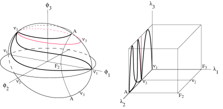
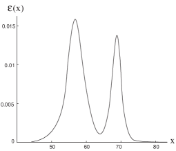
      Figure 4: Solitary waves on $E$ in the Cartesian (left) and elliptic (middle) spaces. Energy density of a kink of the family $T_{E}^{v_{1},v_{3}}$ (right).

    The energy of these solutions can easily be calculated by integrating $dW$ along their respective orbits:

    $$E[T^{v_{1},v_{3}}_{E}] = \int_{T^{v_{1},v_{3}}_{E}}dW=\int dW^{(0,0)}+\int dW^{(0,1)}$$

    $$= \int_{\bar{\sigma}_{3}^{2}}^{\bar{\alpha}^{2}}dW^{0}_{2}+2\int_{\bar{\sigma}_{2}^{2}}^{1}dW^{0}_{3}=\frac{1}{15}\left(\alpha P_{2}(\bar{\alpha}^{2})-\sigma_{3}P_{2}(\bar{\sigma}_{3}^{2})-2\sigma_{2}P_{2}(\bar{\sigma}_{2}^{2})\right)$$

    $$= \frac{2}{3}\left[\left(\frac{\alpha^{5}}{5}-\alpha^{3}\right)-\left(\frac{\sigma_{3}^{5}}{5}-\sigma_{3}^{3}\right)-2\left(\frac{\sigma_{2}^{5}}{5}-\sigma_{2}^{3}\right)\right]$$

    $$E[N^{v_{3}}_{E}] = \int_{N^{v_{3}}_{E}}dW=\int dW^{(0,0)}+\int dW^{(0,1)}+\int dW^{(1,0)}+\int dW^{(1,1)}$$

    $$= 2\int_{\bar{\alpha}^{2}}^{\bar{\sigma}_{2}^{2}}dW_{2}^{0}+4\int_{\bar{\sigma}_{2}^{2}}^{1}dW_{3}^{0}=\frac{1}{15}\left(-2\sigma_{2}P_{2}(\bar{\sigma}_{2}^{2})-2\alpha P_{2}(\bar{\alpha}^{2})\right)$$

    $$= \frac{4}{3}\left[\left(\sigma_{2}^{3}-\frac{\sigma_{2}^{5}}{5}\right)+\left(\alpha^{3}-\frac{\alpha^{5}}{5}\right)\right]$$

  • Solutions on the plane $\phi_{3}=0$.

    In this case, the terms $U_{2}$ and $U_{1}$ of the potential vanish, but not simultaneously. The former vanishes over $\lambda_{2}=\bar{\sigma}_{3}^{2}$, and the latter over $\lambda_{1}=\bar{\sigma}_{3}^{2}$. Because of this, two superpotential functions appear, and hence two systems of differential equations must be involved in order to determine this solution. Nevertheless, we can synthesize $W$ as follows:

    $$W^{(\beta_{k},\beta_{3})}(\lambda_{k},\lambda_{3})=\frac{1}{15}\sum_{i=k,3}(-1)^{\beta_{i}}P_{2}(\lambda_{i})\sqrt{1-\lambda_{i}}\quad,\quad\beta_{i}=0,1,$$

    where $k=1$ for $\lambda_{2}=\bar{\sigma}_{3}^{2}$, and $k=2$ for $\lambda_{1}=\bar{\sigma}_{3}^{2}$. The equations of the orbit on the plane $\lambda_{k}=\bar{\sigma}_{3}^{2}$ are:

    $$e^{2\gamma_{2}}=\prod_{j=1\atop{j\neq 3}}^{4}\left|\frac{\sqrt{1-\lambda_{k}}-\sqrt{1-c_{j}}}{\sqrt{1-\lambda_{k}}+\sqrt{1-c_{j}}}\right|^{\frac{(-1)^{\beta_{k}}(c_{j}-c_{3})}{F_{j}(c)}}\prod_{j=1\atop{j\neq 3}}^{4}\left|\frac{\sqrt{1-\lambda_{3}}-\sqrt{1-c_{j}}}{\sqrt{1-\lambda_{3}}+\sqrt{1-c_{j}}}\right|^{\frac{(-1)^{\beta_{3}}(c_{j}-c_{3})}{F_{j}(c)}}.$$

    Again we have two kinds of solutions:

    • $\,T^{v_{1},v_{2}}_{\sigma_{3}}\,$: Unstable topological solutions linking the vacua $v^{1}$ and $v^{2}$. These solutions leave $v^{1}$, intersect the axis $\phi_{2}$ and the segment $F_{1}F_{3}$ consecutively, and finally arrive at $v^{2}$, as depicted in Figure 5.

    • $\,N^{v_{2}}_{\sigma_{3}}\,$: Unstable non-topological solutions connecting $v^{2}$. The solutions go from $v^{2}$, intersect the axis $\phi_{2}=0$, cross the focus $F_{2}$, and return to the initial point $v^{2}$.

      

      

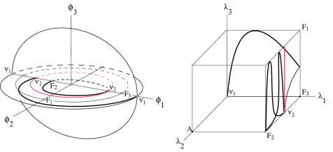
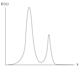
      Figure 5: Solitary waves on $\phi_{3}=0$ in the Cartesian (left) and elliptic (middle) spaces. Energy density of a kink of these families (right).

      The computation of the energies is as follows:

      $$E[T^{v_{1},v_{2}}_{\sigma_{3}}] = \frac{2}{3}\left[\left(\frac{\alpha^{5}}{5}-\alpha^{3}\right)-\left(\frac{1}{5}-\alpha^{2}\right)-2\left(\frac{\sigma_{2}^{5}}{5}-\sigma_{2}^{3}\right)\right]$$

      $$E[N^{v_{2}}_{\sigma_{3}}] = \frac{4}{3}\left[\left(\alpha^{3}-\frac{\alpha^{5}}{5}\right)+\left(\sigma_{2}^{3}-\frac{\sigma_{2}^{5}}{5}\right)\right]\,.$$

  • Solutions on the plane $\phi_{2}=0$, see Figure 6.

    Now, the terms $U_{3}$ and $U_{2}$ of the potential vanish over $\lambda_{3}=\bar{\sigma}_{2}^{2}$ and $\lambda_{2}=\bar{\sigma}_{2}^{2}$, respectively. The two superpotential functions that appear can be synthesized in a similar way:

    $$W^{(\beta_{1},\beta_{k})}(\lambda_{1},\lambda_{k})=\frac{1}{15}\sum_{i=1,k}(-1)^{\beta_{i}}P_{2}(\lambda_{i})\sqrt{1-\lambda_{i}}\ \quad,\quad\beta_{i}=0,1,$$

    where $k=2$ for $\lambda_{3}=\bar{\sigma}_{2}^{2}$ and $k=3$ for $\lambda_{2}=\bar{\sigma}_{2}^{2}$. The equations of the orbit on the plane $\lambda_{k}=\bar{\sigma}_{2}^{2}$ are:

    $$e^{2\gamma_{2}}=\prod_{j=1\atop{j\neq 2}}^{4}\left|\frac{\sqrt{1-\lambda_{1}}-\sqrt{1-c_{j}}}{\sqrt{1-\lambda_{1}}+\sqrt{1-c_{j}}}\right|^{\frac{(-1)^{\beta_{1}}(c_{j}-c_{2})}{F_{j}(c)}}\prod_{j=1\atop{j\neq 2}}^{4}\left|\frac{\sqrt{1-\lambda_{k}}-\sqrt{1-c_{j}}}{\sqrt{1-\lambda_{k}}+\sqrt{1-c_{j}}}\right|^{\frac{(-1)^{\beta_{k}}(c_{j}-c_{2})}{F_{j}(c)}}\,.$$

    We now have three classes of solutions:

    • $T^{v_{1},v_{2}}_{\sigma_{2}}\,$: Stable topological solutions that join the minima $v^{1}$ and $v^{2}$, as can be observed in Figure 6.

    • $T^{v_{3}}_{\sigma_{2}}$: Unstable topological solutions that connect the point $v^{3}$ with the minimum, which is its reflection by the transformation $\phi_{3}\rightarrow-\phi_{3}$, previously crossing the focus $F_{3}$.

    • $T^{v_{2},v_{3}}_{\sigma_{2}}$: Unstable topological solutions that link the points $v^{2}$ and $v^{3}$. In this case, the solutions depart from $v^{2}$, and finally arrive at $v^{3}$ after intersecting the axis $\phi_{3}$.

      

      

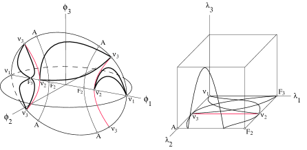
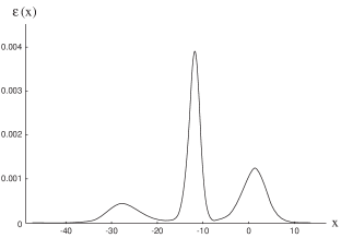
      Figure 6: Solitary waves on $\phi_{2}=0$ in the Cartesian (left) and elliptic (middle) spaces. Energy density of a concrete kink of the family $T_{\sigma_{2}}^{v_{3}}$ (right).

      The energies for these solutions are:

      $$E[T^{v_{1},v_{2}}_{\sigma_{2}}] = \frac{2}{3}\left[\left(\frac{1}{5}-\alpha^{2}\right)-\left(\frac{\alpha^{5}}{5}-\alpha^{3}\right)\right]$$

      $$E[T^{v_{3}}_{\sigma_{2}}] = \frac{4}{3}\left[\left(\frac{1}{5}-\alpha^{2}\right)-\left(\frac{\alpha^{5}}{5}-\alpha^{3}\right)\right],$$

      providing a simple kink energy sum rule: $2E[T^{v_{1},v_{2}}_{\sigma_{2}}]=E[T^{v_{3}}_{\sigma_{2}}]$. The remaining energy is:

      $$E[T^{v_{2},v_{3}}_{\sigma_{2}}]=\frac{2}{3}\left[\left(\frac{\sigma_{3}^{5}}{5}-\sigma_{3}^{3}\right)-2\left(\frac{\alpha^{5}}{5}-\alpha^{3}\right)-\left(\frac{1}{5}-\alpha^{2}\right)\right].$$

    In figure 6(right), we have depicted the energy density $\varepsilon(x)$ of a member of the family $T_{\sigma_{2}}^{v_{3}}$. We notice that the kinks of this family consist of three basic lumps.

  • Solutions on the hyperboloid.

    The term $U_{2}$ vanishes over $\lambda_{2}=\bar{\alpha}^{2}$ and hence the superpotential function is:

    $$W^{(\beta_{1},\beta_{3})}(\lambda_{1},\lambda_{3})=\frac{1}{15}\sum_{i=1,3}(-1)^{\beta_{i}}P_{2}(\lambda_{i})\sqrt{1-\lambda_{i}}\ \quad,\quad\beta_{i}=0,1.$$

    The equation of the orbit is:

    $$e^{2\gamma_{2}}=\prod_{j=2}^{4}\left|\frac{\sqrt{1-\lambda_{1}}-\sqrt{1-c_{j}}}{\sqrt{1-\lambda_{1}}+\sqrt{1-c_{j}}}\right|^{\frac{(-1)^{\beta_{1}}(c_{j}-c_{1})}{F_{j}(c)}}\prod_{j=2}^{4}\left|\frac{\sqrt{1-\lambda_{3}}-\sqrt{1-c_{j}}}{\sqrt{1-\lambda_{3}}+\sqrt{1-c_{j}}}\right|^{\frac{(-1)^{\beta_{3}}(c_{j}-c_{1})}{F_{j}(c)}}.$$

    In this case, only one family is found.

    • $T^{v_{2},v_{3}}_{H}\,$: The trajectories of these stable solutions connect the points $v^{2}$ and $v^{3}$, previously intersecting the plane $\phi_{1}=0$, as is shown in Figure 7. Notice that the energy density in this case comprises two basic lumps.

    The energy is:

    $$E[T^{v_{2},v_{3}}_{H}]=\frac{2}{3}\left[\left(\frac{\sigma_{3}^{5}}{5}-\sigma_{3}^{3}\right)-\left(\frac{1}{5}-\alpha^{2}\right)-2\left(\frac{\sigma_{2}^{5}}{5}-\sigma_{2}^{3}\right)\right]\,.$$

    

    

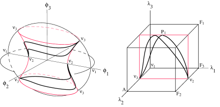
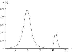
    Figure 7: Solitary waves on $H$ in the Cartesian (left) and elliptic (middle) spaces. Energy density of a kink of this family (right).

• Three-Parametric families of solutions. We find three kinds of solutions:

  • Solutions located inside the ellipsoid and outside the hyperboloid, see Figure 8:

    • $T^{v_{1},v_{2}}\,$: Stable topological solutions that join $v^{1}$ and $v^{2}$. The solutions emerge from $v^{1}$, later cross the plane $\phi_{1}=0$, and finally arrive at $v^{2}$.

    • $T^{v_{3}}\,$: Unstable topological solutions, which start from a minimum $v^{3}$, consecutively cross the planes $\phi_{1}=0$ and $\phi_{3}=0$, intersecting the $F_{1}F_{3}$ edge, and finally arrive at $v^{3}$. Notice that the energy density in this case comprises four basic lumps.

      

      

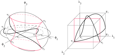
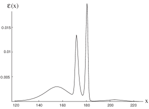
      Figure 8: Generic solitary waves in the Cartesian (left) and elliptic (middle) spaces. Energy density of a kink of the family $T^{v_{3}}$ (right).

      Their energies are:

      $$E[T^{v_{1},v_{2}}] = \frac{2}{3}\left[\left(\frac{\alpha^{5}}{5}-\alpha^{3}\right)-\left(\frac{1}{5}-\alpha^{2}\right)-2\left(\frac{\sigma_{2}^{5}}{5}-\sigma_{2}^{3}\right)\right]$$

      $$E[T^{v_{3}}] = \frac{4}{3}\left[\left(\frac{\alpha^{5}}{5}-\alpha^{3}\right)-\left(\frac{1}{5}-\alpha^{2}\right)-\left(\frac{\sigma_{2}^{5}}{5}-\sigma_{2}^{3}\right)\right]$$

  • Solutions located inside the hyperboloid:

    • $T^{v_{2},v_{3}}\,$: These are unstable solutions. They leave $v^{2}$, cross the plane $\phi_{1}=0$, later intersect the hyperbola $AF_{2}$, cross the plane $\phi_{1}=0$ again, and finally arrive at the point $v^{3}$; see Figure 9.

    

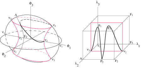
    Figure 9: Generic solitary waves in the Cartesian (left) and elliptic (right) spaces.

    The energy in this case is:

    $$E[T^{v_{2},v_{3}}]=\frac{2}{3}\left[\left(\frac{\sigma_{3}^{5}}{5}-\sigma_{3}^{3}\right)-\left(\frac{1}{5}-\alpha^{2}\right)-2\left(\frac{\sigma_{2}^{5}}{5}-\sigma_{2}^{3}\right)-2\left(\frac{\alpha^{5}}{5}-\alpha^{3}\right)\right]$$

  To complete the previous energy calculations, the kink energy sum rules satisfied by the generic solutions are offered:

  • $E[T^{v_{1},v_{2}}]=E[T^{v_{1},v_{2}}_{\sigma_{3}}]$

  • $2E[T^{v_{2},v_{3}}]=E[N^{v_{3}}_{E}]+E[T^{v_{2},v_{3}}_{H}]+E[T^{v_{2},v_{3}}_{\sigma_{2}}]$

  • $2E[T^{v_{3}}]=E[T^{v_{1},v_{3}}_{E}]+E[T^{v_{2},v_{3}}_{H}]-3E[T^{v_{1},v_{2}}_{\sigma_{2}}]$.

  See Sub-section 3.1 of Reference [16] for an explanation of the origin of these rules in a simpler setting. We stress that the decomposition of the kink energy density in several lumps is due to the kink energy sum rules.

Finally, as an example we depict the kink form factor (Fig. 10 and Fig. 11) for the two unstable generic solutions.

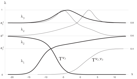
Figure 10: Factor form for the $T^{v_{2},v_{3}}$ and $T^{v_{3}}$ solutions. For the $T^{v_{3}}$ solution, we have taken $\gamma_{1}=0$, $\gamma_{2}=5$ and $\gamma_{3}=-5$, whereas for the $T^{v_{2},v_{3}}$ solution the constants are $\gamma_{1}=\gamma_{2}=\gamma_{3}=0$.

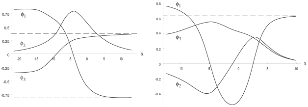
Figure 11: Form factors in the Cartesian space for the $T^{v_{3}}$ and $T^{v_{2},v_{3}}$ solutions

5 Further Comments

It is possible to generalize this kind of model in two senses; we enlarge the internal space with $N$ scalar fields and we include a greater number of coupling constants $\bar{\alpha}_{i}^{2}$.

1. To study the generalization of this kind of system to $N$ dimensions, it is first necessary to introduce $N$-dimensional Jacobi elliptic coordinates. An appropriate explanation of these can be seen in [16]. The potential function we propose for the system is as follows:

$$U(\lambda;\bar{\alpha}^{2})=\sum_{i=1}^{N}U_{i}(\lambda;\bar{\alpha}^{2})=\frac{1}{2}\sum_{i=1}^{N}\frac{\lambda_{i}^{2}(\lambda_{i}-\bar{\alpha}^{2})^{2}\prod_{j=2}^{N}(\lambda_{i}-\bar{\sigma}_{j}^{2})}{f_{i}(\lambda)}\,,$$

where the coupling constants together with the coordinates satisfies the chain

$$-\infty<\lambda_{1}<\bar{\sigma}_{N}^{2}<\lambda_{2}<\ldots<\lambda_{N-1}<\bar{\sigma}_{2}^{2}<\lambda_{N}<1=\bar{\sigma}_{1}^{2}.$$

The denominator is $f_{i}(\lambda)=\prod_{j\neq i}^{N}(\lambda_{i}-\lambda_{j})$, and $\bar{\alpha}^{2}$ is a real positive constant. The function $U(\lambda;\bar{\alpha}^{2})$ is positive semi-definite and presents a number of zeroes, depending on $\bar{\alpha}^{2}$. The most interesting kink manifold appears when $\bar{\alpha}^{2}\in L_{i}\,,\,i=1,\ldots,N$, and becomes richer as $i$ increases, the $L_{i}$ intervals being the trivial generalization of those appearing in the three-dimensional potential.

We shall now briefly study the vacuum manifold in all the $N$ different cases at once. Let us set $\bar{\alpha}^{2}$ such that $\bar{\alpha}^{2}\in L_{j}$ for some $j$ between $1$ and $N$. To find a zero of the function $U(\lambda;\bar{\alpha}^{2})$, we must make every term $U_{i}(\lambda;\bar{\alpha}^{2})$ vanish. To visualize the process, we shall seek help from the following graphic

Each circle in the $\lambda_{k}$ block represents a value that $\lambda_{k}$ can take to make the term $U_{k}(\lambda;\bar{\alpha}^{2})$ null. Each value appearing in the vacuum coordinates will be represented by a full circle, and hence each vacuum in the elliptic space is represented by $N$ full circles. To fill the $N-j$ circles to the right of $\bar{\alpha}^{2}$, there is only one possibility, as seen in the figure, but to fill the remaining $j$ circles we have a number of different ways equal to the number of permutations of $j+1$ elements, $j$ of them being repeated. Therefore, we have $P^{(j+1)}_{j,1}=j+1$ zeroes of the $U(\lambda;\bar{\alpha}^{2})$ function, $j$ of them being on the plane $\lambda_{j}=\bar{\alpha}^{2}$. To figure out the number of corresponding Cartesian vacua, we only need to take into account the multiplicity of each elliptic vacuum. By doing this, we conclude that by introducing a regular plane $\lambda_{j}=\bar{\alpha}^{2}$ there are ${\cal V}=4+(j-1)2^{N-1}$ Cartesian vacua. The kink manifold thus decomposes into ${\cal V}^{\,2}$ disconnected sectors [7].

2. The second generalization considers not only one parameter, $\bar{\alpha}^{2}$, but several of them. The generalized potential is constructed as follows.

Let us consider numbers $n_{i}=0,1,2,\ldots$ with $i=1,\ldots,N$, and let us define $(n_{1}+\ldots+n_{N})$ different parameters $\bar{\alpha}^{2}_{ij}$, such that for each $n_{i}\neq 0$, $\bar{\alpha}^{2}_{ij}\in L_{i}$ and $j=1,\ldots,n_{i}$. We can therefore construct the $N$-dimensional potential:

$$U=\sum_{i=1}^{N}U_{i}(\lambda,\bar{\alpha}_{ij}^{2})=\frac{1}{2}\sum_{i=1}^{N}\frac{\lambda_{i}^{2}(\lambda_{i}-\bar{\sigma}_{2}^{2})(\lambda_{i}-\bar{\sigma}_{3}^{2})}{f_{i}(\lambda)}\prod_{j=1\atop{n_{i}\neq 0}}^{n_{i}}(\lambda_{i}-\bar{\alpha}^{2}_{ij})^{2}\,.$$ (22)

The case in which $\sum_{i=1}^{N}n_{i}=0$ corresponds to the deformed $O(N)$ linear sigma model [16] and the case $\sum_{i=1}^{N}n_{i}=1$, with $N=3$, is precisely the model studied in the previous sections.

As $\sum_{i=1}^{N}n_{i}$ increases, the vacuum manifold becomes more and more abundant owing to the appearance of an increasing number of roots in the potential. An easy way to account for the vacuum manifold ${\cal V}$ is through the corresponding generalization of the previous graphic

In this picture $(n_{1}+\dots+n_{N})$ additional circles appear, $\alpha$-holes for short, since every $\bar{\alpha}_{ij}^{2}$ is easily seen to be a root of the $U_{i}$ term in (22). Computation of the number of vacua now proves to be an easy task given that, as before, each vacuum point is represented by $N$ filled circles. It happens that the number of vacua -including $v_{1}$, which corresponds to all the $\alpha$-holes emptied- is given by:

$$\textnormal{Card}({\cal V})=1+\sum_{q=1}^{N}N_{q}\,,$$

where $N_{q}$ is the number of vacuum points with $q$ filled $\alpha$-holes, which can be calculated readily using combinatorial techniques.

Regarding the kink manifold, and looking at the corresponding first-order equations, for each $\bar{\alpha}^{2}_{ij}$ we can deduce a confinement of the solutions in $\bar{P}_{3}(0)$ similar to that obtained in section 3. Therefore, a number of $2^{(n_{1}+\ldots+n_{N})}$ subsets of $\bar{P}_{3}(0)$ that host general kink solutions appear.

The purpose of this construction is now clear. Recalling the stability criterion and the confinement of the solutions due to the factors $(\lambda_{i}-\bar{\alpha}^{2}_{ij})^{2}$, we can isolate the edges $F_{1}F_{3}=\{\bar{\sigma}_{3}^{2},\bar{\sigma}_{3}^{2},\lambda_{3}\}$ and $AF_{2}=\{\lambda_{1},\bar{\sigma}_{2}^{2},\bar{\sigma}_{2}^{2}\}$. Proceeding in this way, we can find subsets of the configuration space in which only stable solutions emerge.

Acknowledgements

The authors warmly acknowledge many discussions with J. Mateos Guilarte. A.A.I. thanks the Secretaria de Estado de Educación y Universidades of Spain for financial support.

References

References

- [1] R. Rajaraman, Solitons and instantons. An introduction to solitons and instantons in quantum field theory, North-Holland Publishing Co., Amsterdam, 1982
- [2] C. Montonen, Nucl. Phys. B112 (1976) 349–357 S. Sarker, S.E. Trullinger and A.R. Bishop, Phys. Lett. A59 (1976) 255-258 K.R. Subbaswamy and S.E. Trullinger, Physica D2 (1981) 379-388
- [3] E. Magyari and H. Thomas, Phys. Lett. A100 (1984) 11–14
- [4] H. Ito, Phys. Lett. A112 (1985) 119-123
- [5] H. Ito and H. Tasaki, Phys. Lett. A113 (1985) 179-182
- [6] J. Mateos Guilarte, Lett. Math. Phys. 14 (1987) 169–176 J. Mateos Guilarte, Ann. Phys. 188 (1988) 307–346
- [7] A. Alonso Izquierdo, M.A. González León and J. Mateos Guilarte, J. Phys. A31 (1998) 209-229
- [8] A. Perelomov, “Integrable Systems of Classical Mechanics and Lie Algebras”, Birkhäuser, Boston MA., 1990
- [9] R. Garnier, Ren. Circ. Mat. Palermo 43 (1919) 155–191
- [10] D. Bazeia, J.R.S. Nascimento, R.F. Ribeiro and D. Toledo, J. Phys. A30 (1997) 8157-8166 D. Bazeia, H. Boschi-Filho and F.A. Brito, JHEP 9904 (1999) 028
- [11] A. Alonso Izquierdo, M.A. González León and J. Mateos Guilarte, Phys. Rev. D65 (2002) 085012
- [12] M. Shifman and M. Voloshin, Phys. Rev. D 57 (1998) 2590
- [13] A. Alonso Izquierdo, M.A. González León, J. Mateos Guilarte and M. de la Torre Mayado, Phys. Rev. D66 (2002) 105022
- [14] S. Cecotti, C. Vafa, Comm. Math. Phys. 158 (1993) 569–644 P. Fendley, S.D. Mathur, C. Vafa, and N.P. Warner, Phys. Lett. B243 (1990) 257–264
- [15] A. Alonso Izquierdo, M.A. González León and J. Mateos Guilarte, Phys. Lett. B480 (2000) 373-380
- [16] A. Alonso Izquierdo, M.A. González León and J. Mateos Guilarte, Nonlinearity, 13 (2000) 1137-1169
- [17] A. Alonso Izquierdo, M.A. González León and J. Mateos Guilarte, Nonlinearity, 15 (2002) 1097-1125
- [18] A. Alonso Izquierdo, M.A. González León and J. Mateos Guilarte and M. de la Torre Mayado, Ann. Phys. 308 (2003) 664-691