Modelling of quantum networks

Abstract

Mathematical design of a quantum network with prescribed transport properties is equivalent to the Inverse Scattering Problem for Schrödinger equation on a composite domain consisting of quantum wells and finite or semi-infinite quantum wires attached to them. An alternative approach to study of transport properties of networks, based on solution of the direct Scattering problem, is also possible, but optimization of design requires scanning over the multi-dimensional space of essential physical and geometrical parameters of the network. We propose a quantitatively consistent description of one-particle transport in the network based on observation that the transmission of an electron across the wells, from one quantum wire to the other, happens due to the excitation of oscillatory modes in the well. This approach permits us to obtain an approximate formula for the transmission coefficients based on numerical data for eigenvalues and eigenfunctions of the discrete spectrum of some intermediate Schrödinger operator on the network in certain range of energy. The obtained approximate formula for the transmission coefficients permits to reduce the region of search in the space of parameters in course of optimization of the design. We interpret the corresponding approximate Scattering matrix as a Scattering matrix of the relevant solvable model which can be used when modelling the network by a quantum graph.

I Introduction

Modern interest to quantum networks is inspired by the engineering of quantum electronic devices and oriented to manufacturing of networks with prescribed transport properties. In simplest case of a single-particle, single-mode processes transport properties can be described in terms of Scattering. Quantum conductance was related to Scattering Processes in pioneering papers by Landauer and Büttiker, see Landauer70 ; Buttiker85 , and the role of the resonance scattering in mathematical design of quantum electronic devices was clearly understood by the beginning of the nineties, see Adamyan ; BH91 ; Buttiker93 .Nevertheless practical design of devices up to now, see for instance Compano , was based on the formal resonance of energy levels rather than on resonance properties of the corresponding wave functions. At the same time importance of interference in mathematical design of devices was noticed in Exner88 ; Alamo and intensely studied in PalmThil92 ; Exner96 ; Interf1 ; Interf2 , see also recent papers Safi99 ; Aver_Xu01 ; ScattXu02 ; Kouw2002 .

Experimental technique already permits to observe resonance effects caused by the shape of the resonance wave functions, see B1 ; B2 ; Carbon01 . In our previous papers, see for instance Helsinki2 ; PRB ; boston , we proposed using the shape resonance effects as a tool for manipulation of the quantum current. In particular, we considered the process of resonance transmission of an electron in the switch across the quantum well from one quantum wire to another based on excitation of resonance modes inside the vertex domain- a phenomenon which was first mathematically described in Opening .

In actual paper we apply this basic idea to description of one-electron transmission in general quantum networks which can be formed on the surface of a semiconductor of quantum wells and quantum wires joining them or connecting them to infinity. The depth of the wires and the wells with respect to the potential on the complement of the network is assumed large enough to replace the matching boundary conditions on the boundary of the network by homogeneous Dirichlet conditions for electrons with energy close to the Fermi level $E_{{}_{F}}=\Lambda$ in the wires, see Madelung . The limitations we impose on the width $\delta$ of the wires are practically not too strict. They are defined from comparison of the non-dimensional wave-number of electron in the wires on Fermi level $\Lambda$ and the non-dimensional inverse spacing between eigenvalues of an intermediate operator on the resonance level $\lambda\approx\Lambda$. The numerical analysis of the circular quantum switch, see boston , shows that our approximation is applicable to the network constructed of a circular vertex domain with diameter $d$ and quantum wired width $\delta$ submitted to the condition $d\geq 4\delta$. Hence our further assumptions on the width of the wires do not mean actually that the wires are “thin” or the connection of the wires to the quantum wells is weak, though we include below, lemma 3.1, also analysis of this case. We assume that the dynamics of the electrons in the wires is single-mode and ballistic on large intervals of the wires compared with the size of geometric details of the construction (the width of the wire or the size of the contacts). Our methods in this paper are based on analysis of the one-body scattering problem for the relevant Schrödinger equation on the network.

A general Quantum network which is studied in this paper is a composite domain of a sophisticated form, a sort of a “fattened graph”, see for instance KZ01 . It is impossible to obtain an explicit solution of the Schrödinger equation on this domain in analytic form. On the other hand, the direct computation is not efficient for optimization of the construction of the network with prescribed transport properties, because the resonance transmission effect is observed only at a multiple point in the space of geometrical and physical parameters.

Substitution of the network by proper one-dimensional graph with special boundary conditions at the vertices looks like an attractive program aimed to obtaining explicit formulae for solutions of the Schrödinger equation on the network, see Gerasimenko ; Novikov ; Schrader ; MP00 . Really, analysis of the one-dimensional Schrödinger equation on the graph , or even on some hybrid domain as in MP01 ; MPP02 is a comparatively simple mathematical alternative, but estimation of the error appearing from the substitution of the network by a corresponding graph is difficult. Asymptotic behavior of discrete spectrum in composite domains with shrinking channels was studied in Jimbo see also references therein. Simultaneous shrinking joining channels and vertex domains of a realistic compact network was studied in extended series of papers on the edge of last century. In particular in KZ01 ; RS01 the authors develop, based on Schat96 , a variational technique for discrete spectrum of Schrödinger operator on a “fattened graph”. They noticed that the (discrete) spectrum of the Laplacian on a system of finite length shrinking wave-guides, width $\varepsilon$, attached to the shrinking vertex domain diameter $\varepsilon^{\alpha},\,0<\alpha<1$ tends to the spectrum of the Laplacian on the corresponding one-dimensional graph but with different boundary conditions at vertices depending on speed of shrinking. In case of “small protrusion” $1/2<\alpha<1$ the spectrum in the corresponding composite domain tends to the spectrum on a graph with Kirchhoff boundary conditions at vertices; for the intermediate case $\alpha=1/2$ the boundary condition becomes energy-dependent, and for “large protrusion”, $0<\alpha<1/2$, the spectrum on a system of wave-guides, when shrinking, tends to the spectrum on the graph with zero boundary conditions at the points of contact so the vertices play the role of “black holes” according to KZ01 .

In distinction from the papers KZ01 ; RS01 quoted above, our theoretical analysis of the Schrödinger equation on the “fattened graph” P02 was based on a single-mode one-body scattering problem in the corresponding composite domain with several semi-infinite wires. The aim of actual paper is: an “approximate” description of transport properties of the network. We achieve this aim via derivation of an explicit formula for the Scattering Matrix in terms of the Dirichlet-to-Neumann map of a specific intermediate operator obtained via proper splitting ( see Glazman ) of the relevant Schrödinger operator ${\cal L}$ on the whole network in a certain interval of energy. Construction of the system of intermediate operators $\left\{L_{{}_{\Lambda}}\right\}$ is defined by the band structure of the absolutely continuous spectrum $\sigma_{{}_{a}}$ of the Schrödinger operator on the network the following way.

The multiplicity $n=n_{{}_{\lambda}}$ of the absolutely continuous spectrum of the Schrödinger operator on the network is finite on each finite interval. If the Fermi level $E_{{}_{F}}=\Lambda$ is sitting on the spectral band $\Delta_{n}=\left[T_{n},\,\,T_{n+1}\right]$ with the spectral multiplicity $n=n(\Lambda)$, then the specific splitting ${\cal L}\longrightarrow{\cal L}_{{}_{\Lambda}}={L}_{{}_{\Lambda}}\oplus l_{{}_{\Lambda}}$ is applied to the Schrödinger operator on the whole network to create the Intermediate operator ${L}_{{}_{\Lambda}}$, defined in the orthogonal complement of “open channels” in the wires, see section 2. When matching the outgoing solutions of the corresponding intermediate Schrödinger equation with exponentials in the chopped-off open channels, we obtain scattered waves of the Schrödinger operator on the whole quantum network and calculate the corresponding Scattering matrix. The eigenvalues of the intermediate operators $L_{{}_{\Lambda}}$ below the threshold $T_{n+1}$ generically give rise to resonances of the Schrödinger operator on the whole network, see the formulae (23) and (36) below, or become embedded eigenvalues. In simplest case,when just one quantum well with four equivalent wires attached is involved, see boston , and only one simple resonance eigenvalue $\lambda_{{}_{0}}^{{}^{\Lambda}}$ of the Intermediate operator is sitting on the first spectral band $\Delta_{4}$, close to the Fermi-level $\Lambda$, the Scattering matrix is presented approximately by the corresponding resonance factor (1). This factor contains the pole of the ${\cal D}{\cal N}$-map at the resonance eigenvalue and the normal derivatives of the corresponding eigenfunction $\varphi_{0}$ projected onto the corresponding four-dimensional entrance subspace $E^{{}^{\Lambda}}_{{}_{+}}=E_{{}_{+}}$ of the open channels,- the linear hull of the corresponding cross-section eigenfunctions in the wires:

$$S(\lambda)=-\frac{{\cal D}{\cal N}^{{}^{\Lambda}}+iK_{+}}{{\cal D}{\cal N}^{{}^{\Lambda}}-iK_{+}}\approx$$

$$-\frac{\frac{P_{+}\frac{\partial\varphi_{{}_{0}}(x)}{\partial n_{x}}\rangle\,\,\langle P_{+}\frac{\partial\varphi_{{}_{0}}(s)}{\partial n_{s}}}{\lambda-\lambda^{{}^{\Lambda}}_{{}_{0}}}+iK_{+}(\lambda^{{}^{\Lambda}}_{0})}{\frac{P_{+}\frac{\partial\varphi_{{}_{0}}(x)}{\partial n_{x}}\rangle\,\,\langle P_{+}\frac{\partial\varphi_{{}_{0}}(s)}{\partial n_{s}}}{\lambda-\lambda^{\Lambda}_{0}}-iK_{+}(\lambda^{{}^{\Lambda}}_{0})}.$$ (1)

Here $K_{{}_{+}}$ is the exponent obtained from oscillatory solutions in semi-infinite quantum wires and $P_{+}\frac{\partial\varphi_{{}_{0}}(x)}{\partial n_{x}}\rangle\,\,\langle P_{+}\frac{\partial\varphi_{0}(s)}{\partial n_{s}}$ is the resonance term associated with the resonance eigenvalue $\lambda^{{}^{\Lambda}}_{{}_{0}}$ and the corresponding eigenfunction $\varphi_{0}$. It can be presented in standard form $\parallel P_{+}\frac{\partial\varphi_{0}}{\partial n}\parallel^{2}P_{0}$ with the orthogonal projection $P_{0}$ onto the one-dimensional subspace $E^{{}^{0}}_{+}$ in $E_{+}$ spanned by $P_{+}\frac{\partial\varphi_{0}}{\partial n}$.

The above “one-pole” approximation (1) of the Scattering matrix near the resonance eigenvalue $\lambda^{{}^{\Lambda}}_{{}_{0}}$ is obtained via substitution of the Dirichlet-to-Neumann map of the intermediate operator by the resonance term only, neglecting all non-resonance terms and the contribution from the continuous spectrum. In case of the resonance triadic Quantum Switch, see boston , similar neglecting was possible in a small neighborhood of the resonance eigenvalue. The size of the neighborhood was defined by the “natural” small parameter $\approx 1/20$ which appears from above mentioned comparison of the inverse spacing of eigenvalues of the intermediate operator on the resonance level and the wave-number of the electron in the wire on the resonance energy. We derive also a “few-pole approximation” of the Scattering matrix and interpret it as a Scattering matrix of some solvable model of the network in certain range of energy.

Actual paper has the following plan: after the formal description of the quantum network and introduction of an intermediate operator in the next section 2, we prove in section 3 that the intermediate operator $L_{\Lambda}$ is self-adjoint, hence possess a resolvent kernel which has usual properties.Based on these properties we introduce the corresponding Dirichlet-to-Neumann map of the Intermediate operator and connect it with the Dirichlet-to-Neumann map of the Schrödinger operator on the Quantum well. The following section 4 contains the calculation of the Scattering matrix and derivation of the corresponding “one-pole approximation”. Then in section 5 we suggest an interpretation of the “one-pole approximation”of the Scattering matrix on Quantum network as a Scattering matrix of a solvable model presented as a star-shaped graph with a single resonance node. In the last section we discuss briefly some historic details of the perturbation theory on the continuous spectrum.

The aim of our paper is the description of an approach to the transport problem on the network based on the idea of the intermediate operator. This approach is demonstrated in details. But the total volume of this paper is not sufficient to discuss all subtle mathematical details of each technical step. Hence in couple of places, which are clearly indicated, see for instance discussion of the singular spectrum in Theorem 3.1, we supply just a sketch of the corresponding proof. We plan to return to these questions soon in following publications.

II Intermediate Operators

Consider a network on a plane manufactured of several non-overlapping quantum wells (vertex domains) $\Omega_{t},\,\,t=1,2,\dots T$ and a few straight finite or semi-infinite wires $\omega^{m},\,\,l=1,2,\dots M$ of constant width $\delta_{m}$ and length $d_{m}\leq\infty$ attached to the domains $\Omega_{t_{1}},\,\,\Omega_{t_{2}},\dots$ such that the bottom sections $\gamma^{m}_{t_{1}},\,\gamma^{m}_{t_{2}}$ of the wire $\omega^{m}$ are parts of the piece-wise smooth boundaries $\partial\Omega_{t_{1}},\,\,\partial\Omega_{t_{2}},\dots$ of the domains $\Omega_{t_{1}},\,\,\Omega_{t_{2}},\dots$ respectively. Each wire is attached to one (if the wire is semi-infinite ) or two domains (if it is finite), so that the function $m\to t$ or $m\to t_{1},t_{2}$ is defined although the inverse function may not be defined, since there may be a few wires $\omega^{m}$ connecting two given domains $\Omega_{t_{1}},\,\Omega_{t_{2}}$. In our further construction we use slightly extended vertex domains with small “cut-off’s” $\delta\omega^{{}^{m}}$ of the wires $\omega^{{}^{m}}$ attached to them: $\delta\omega^{{}^{m}}=\left\{0<x<\varepsilon^{{}^{m}}\right\}$, to avoid a discussion of the subtle question of Sobolev smoothness of restrictions of elements from the domain of the operator onto the bottom sections of channels joining the inner angles. Denote by $\gamma^{{}^{m}}_{{}_{t}}$ the orthogonal bottom sections of the “shortened” wires with cut-off’s removed (from both ends,if the wire is finite) and attached to the corresponding vertex domains. We will use further former notations $\Omega_{{}_{t}},\,\omega^{{}^{m}}$ for extended vertex domains and for the shortened wires respectively. The previously described vertex domains and wires will not be used in the following text. We consider the spectral problem for the Schrödinger operator

$${\cal L}u=-\bigtriangleup_{\mu}u+V(x)u=\lambda u$$ (2)

on the network $\Omega=\cup_{t}\Omega_{t}\cup_{m}\omega^{m}$ with zero boundary condition on $\partial\Omega$. The kinetic term $-\bigtriangleup_{\mu}$ containing the tensor $\mu$ of effective mass is defined as

$$-\bigtriangleup_{\mu}=\left\{\begin{array}[]{cc}-(2\mu_{t})^{-1}\bigtriangleup,&\mbox{if}\,\in\Omega_{t}\\ -\frac{1}{2\mu^{{}^{\parallel}}_{{}_{m}}}\frac{\partial^{2}}{\partial x^{2}}-\frac{1}{2\mu^{{}^{\bot}}_{{}_{m}}}\frac{\partial^{2}}{\partial y^{2}}&\mbox{if}\,\in\omega^{m}\end{array}\right.,$$

where $\mu_{t}$ plays the role of the average effective mass in the well $\Omega_{t}$, $x,y$ are the coordinates along and across the wire $\omega^{m}$ and $\mu^{{}^{\bot}}_{{}_{m}},\,\mu^{{}^{\parallel}}_{{}_{m}}$ are positive numbers playing the roles of effective masses across and along the wire $\omega^{m}$ respectively. We impose the Meixner condition at the inner corners of the boundary of the domain in form $D({\cal L})\subset W_{2}^{1}(\Omega)$. We assume that the potential $V$ is constant on the wires $V\bigg{|}_{\omega^{{}^{m}}}=V_{m}$ and is a real bounded measurable function $V_{t}$ on each (extended) vertex domain $\Omega_{t}$. Without loss of generality we may assume that the overlapping wires do not interact, otherwise we may treat the overlapping as an additional quantum well. The absolutely-continuous spectrum of the operator ${\cal L}$ coincides with the absolutely- continuous spectrum of the restriction $\sum_{m=m(t)}\oplus l_{m}$ of the operator ${\cal L}$ onto the sum of all semi-infinite wires $\omega^{m},\,\,m=m(t)$ with zero boundary conditions on the boundary $\cup_{m}\partial\omega^{m}$. This fact follows from the Glazman’s splitting technique, Glazman , see a discussion in the proof of theorem 3.1 in the next section. The spectrum of the restriction $l_{m}$ consists of a countable number of branches $\cup_{m=1}^{\infty}\left[\left.V_{{}_{m}}+\frac{s^{2}\pi^{2}}{2\mu^{{}^{\bot}}_{{}_{m}}\delta^{2}_{m}},\,\infty\right.\right)$ which correspond to the oscillating modes $\displaystyle e^{m}_{s}(y)\,\,\mbox{exp}\pm i\,\sqrt{2\mu^{{}^{\parallel}}_{{}_{m}}}\sqrt{\lambda-\left[V_{{}_{m}}+\frac{s^{2}\pi^{2}}{2\mu^{{}^{\bot}}_{{}_{m}}\delta^{2}_{m}}\right]}\,\,\,x,\,\,\,V_{{}_{m}}+\frac{s^{2}\pi^{2}}{2\mu^{{}^{\bot}}_{{}_{m}}\delta^{2}_{m}}\,\,\,<\,\lambda\,$ spanned by the eigenfunctions of the cross-section $\displaystyle e^{m}_{s}(y)=\sqrt{\frac{2}{\sqrt{2\mu^{{}^{\bot}}_{{}_{m}}}\delta_{m}}}\sin\frac{s\pi y}{\sqrt{2\mu^{{}^{\bot}}_{{}_{m}}}\delta_{m}},\,\,s=1,2,\dots$. If the Fermi-level $\Lambda$ does not coincide with any threshold, $\Lambda\neq V_{{}_{m}}+\frac{s^{2}\pi^{2}}{2\mu^{{}^{\bot}}_{{}_{m}}\delta^{2}_{m}},\,\,s=1,2,\dots$, then the linear hulls of eigenfunctions of the cross-sections corresponding to the open channels $V_{{}_{m}}+\frac{s^{2}\pi^{2}}{2\mu^{{}^{\bot}}_{{}_{m}}\delta^{2}_{m}}<{\Lambda}$ are considered as entrance subspaces of “open (lower) channels”: $E^{m}_{+}(\Lambda)=\bigvee_{s\pi\leq\sqrt{2\mu^{{}^{\bot}}_{{}_{m}}(\Lambda-V_{{}_{m}})}\,\delta_{m}}e^{m}_{s}$. The entrance subspaces of “closed (upper) channels” $E^{m}_{-}(\Lambda)=\bigvee_{s\pi>\sqrt{2\mu^{{}^{\bot}}_{{}_{m}}(\Lambda-V_{{}_{m}})}\,\delta_{m}}e^{m}_{s}=L_{2}(\gamma^{m})\ominus E^{m}_{+}(\Lambda)$, correspond to the upper thresholds: $\frac{s^{2}\pi^{2}}{2\mu^{{}^{\bot}}_{{}_{m}}\delta^{2}_{m}}+V_{{}_{m}}>\Lambda$. Denote by $P^{m}_{\pm}(\Lambda)$ the orthogonal projections onto the subspaces $E^{m}_{\pm}(\Lambda)\subset L_{2}(\gamma^{m}_{t})$ on the bottom sections of the finite and/or infinite wires $\omega^{m}$ lying on the border of the (extended) vertex domain $\Omega_{t}$.

An important feature of the above quantum network is the “step-wise” structure of the continuous spectrum of the operator ${\cal L}$ with spectral bands of different spectral multiplicities separated by thresholds, see Kopilevich . This property permits us to introduce the corresponding structure of intermediate operators.

Note that elements from the domain of the Schrödinger operator ${\cal L}$ on the whole network $\Omega$ belong locally (outside a small neighborhood of inner corners) to the proper Sobolev class $D({\cal L})\subset W_{{}_{2}}^{{}^{2}}(\Omega_{t},loc)$, see KL88 . For given Fermi level $\Lambda>0$ we define an intermediate operator,   following Helsinki2 ; boston ; PRB where the suggested construction was introduced for star-shaped Quantum Switch. The intermediate operator is defined by the same differential expression as the Schrödinger operator ${\cal L}$ defined on $W^{{}^{2}}_{{}_{2}}$-smooth functions in the orthogonal sum of spaces of all square-integrable functions on the components $\left\{\omega^{m},\,\Omega_{t}\right\}$ of the network with special boundary conditions at the bottom sections $\gamma^{m}\in\partial\Omega_{t},\,t=1,2,\dots$ of the wires $\omega^{m}$:

$$P^{m}_{+}(\Lambda)u_{t}\bigg{|}_{\gamma^{m}_{t}}=0,\,\,\,\,\,P^{m}_{+}(\Lambda)u^{m}\bigg{|}_{\gamma^{m}_{t}}=0$$

$$P^{m}_{-}(\Lambda)\left[u^{m}\bigg{|}_{\gamma^{m}_{t}}-u_{t}\bigg{|}_{\gamma^{m}_{t}}\right]=0,\,\,\,\,\,P^{m}_{-}(\Lambda)\left[\frac{1}{2\mu_{m}^{{}^{\parallel}}}\frac{\partial u^{m}}{\partial n}\bigg{|}_{\gamma^{m}_{t}}-\frac{1}{2\mu_{{}_{t}}}\frac{\partial u_{t}}{\partial n}\bigg{|}_{\gamma^{m}_{t}}\right]=0.$$ (3)

These boundary conditions are meaningful due to Embedding theorems, see Embedding , because functions from both $W_{2}^{2}(\Omega_{t},loc),\,\,W_{2}^{2}(\omega^{m})$ have boundary values in proper sense on the elements of the common boundary $\partial\omega^{m}\cap\partial\Omega_{t}$ - on the bottom sections $\gamma_{{}_{t}}^{{}^{m}}$ of the (shortened) wires. We also assume that the Meixner conditions are fulfilled at the inner corners for the component $u_{{}_{t}}$ of the element in the vertex domains. The obtained split operator is denoted further in this section by $\hat{\cal L}_{{}_{\Lambda}}$, and the whole domain of it in $\cup_{{}_{t}}W_{2}^{2}(\Omega_{t},loc)\oplus\cup_{{}_{m}}W_{2}^{2}(\omega^{m})$ is denoted by $D\left(\hat{\cal L}_{{}_{\Lambda}}\right)$. The Meixner condition can be presented as $D\left(\hat{\cal L}_{{}_{\Lambda}}\right)\subset W_{{}_{2}}^{{}^{1}}(\Omega)$.

To present the above boundary conditions in a more compact form we can introduce orthogonal sums of upper (closed) and lower (open) entrance spaces $\sum_{m}\oplus\left(E^{m}_{t}\right)_{{}_{\pm}}:=E_{t,\pm}$ on the wires attached to the domain $\Omega_{t}$. We introduce also similar notations for the corresponding projections $P_{t,\pm}{\bf u}^{\omega}$ of the vectors $\sum_{m}u^{m}:={\bf u}_{t}^{\omega}$ obtained via restriction of functions defined on the wires attached to the given domain $\Omega_{t}$ onto the bottom sections $\gamma_{t}^{m}\in\partial\Omega_{t}\cap\partial\omega^{m}$. Similarly we can introduce the restrictions of the functions $u_{t}$ defined in $\Omega_{t}$ onto the sum $\Gamma_{t}=\cup_{m}\gamma_{t}^{m}$ of all bottom sections $\gamma_{t}^{m}$ of the wires $\omega^{m}$ attached to the domain $\Omega_{t}$:

$${\bf u}_{{}_{{}_{\Omega_{t}}}}=u_{t}\bigg{|}_{{}_{{}_{\Gamma_{t}}}}$$

and the corresponding projections $\sum_{{}_{m}}P^{{}^{m}}_{{}_{t,\,\pm}}=P_{{}_{t,\,\pm}}$, and then form an orthogonal sum:

$${\bf u}_{{}_{{}_{\Omega}}}=\sum_{t}\oplus u_{{}_{\Omega_{t}}},\,\,P_{\pm}{\bf u}_{{}_{{}_{\Omega}}}=\sum_{t,m}\oplus P^{{}^{m}}_{{}_{t,\pm}}{\bf u}_{{}_{\Omega_{t}}}.$$

Now the above boundary conditions can be re-written in a compact form as

$$P_{+}{\bf u}_{{}_{{}_{\Omega}}}=P_{+}{\bf u}^{\omega}=0,\,\,P_{-}\left[{\bf u}_{{}_{{}_{\Omega}}}-{\bf u}^{\omega}\right]=0,\,\,P_{-}\left[\frac{1}{2{\bf\mu}_{{}_{\Omega}}}\frac{\partial{\bf u}_{{}_{{}_{\Omega}}}}{\partial n}-\frac{1}{2{\bf\mu}^{{}^{\parallel}}}\frac{\partial{\bf u}^{\omega}}{\partial n}\right]=0.$$ (4)

Here $\mu_{\Omega},\,\mu^{\parallel}$ are diagonal tensors composed of values of the average effective masses in domains $\Omega_{t}$ and along the wires $\omega^{m}$ respectively. The boundary condition 4 may be interpreted as a “chopping-off” condition in all open (lower) channels $\frac{s^{2}\,\pi^{2}}{2\mu^{\bot}_{{}_{\omega}}\delta_{m}^{2}}+V_{{}_{m}}<\Lambda$ and a “partial matching condition” in all closed (upper) channels $\frac{s^{2}\,\pi^{2}}{2\mu^{\bot}_{{}_{\omega}}\delta_{m}^{2}}+V_{{}_{m}}>\Lambda$. The restrictions $\hat{l}^{m}(\Lambda)$ of the split operator $\hat{\cal L}$ onto the invariant subspaces ${\cal H}^{m}_{+}=\bigvee_{\frac{s^{2}\,\pi^{2}}{2\mu^{\bot}_{{}_{\omega}}\delta_{m}^{2}}+V_{{}_{m}}<\Lambda}e^{m}_{s}\times L_{2}(0,\,d_{m})=E^{m}_{+}\times L_{2}(0,\,d_{m})$ which correspond to the (open) channels $\frac{s^{2}\,\pi^{2}}{2\mu^{\bot}_{{}_{\omega}}\delta^{2}_{m}}+V_{{}_{m}}<\Lambda$, are self-adjoint operators and admit spectral analysis in explicit form. We denote by $\hat{l}_{{}_{\Lambda}}$ the orthogonal sum of all operators $\hat{l}^{{}^{m}}_{{}_{s}}(\Lambda)$ in all open channels. The restriction $\hat{L}_{\Lambda}$ of $\hat{\cal L}$ onto the complementary invariant subspace is also a self-adjoint operator :

$$\hat{L}_{\Lambda}=\hat{\cal L}\,\ominus\,\left\{\sum_{\frac{s^{2}\,\pi^{2}}{2\mu^{\bot}_{{}_{\omega}}\delta^{2}_{m}}+V_{{}_{m}}<\Lambda}\,\,\,{\oplus}\,\,\,\hat{l}^{{}^{m}}_{{}_{s}}(\Lambda)\right\}:=\hat{\cal L}\,\ominus\,\hat{l}_{{}_{\Lambda}}.$$

The above chopping-off construction can be applied either to open channels in all wires, both finite and infinite, resulting in the above operators $\hat{L}_{{}_{\Lambda}}$ and $\hat{l}_{{}_{\Lambda}}$, or applied to the semi-infinite open channels only, resulting in corresponding operators $L_{{}_{\Lambda}},\,\,\,l_{{}_{\Lambda}}$ respectively, ${\cal L}_{{}_{\Lambda}}=L_{{}_{\Lambda}}\,\oplus\,l_{{}_{\Lambda}}$. One of the intermediate operators : $\hat{L}_{\Lambda}$ or $L_{{}_{\Lambda}}$ can be more convenient for calculating the Scattering matrix, depending on the architecture of the network. In the remaining part of this paper we choose $L_{{}_{\Lambda}}$ as an intermediate operator, chopping off only the open channels in semi-infinite wires.

Some useful modification of the above chopping-off construction is also convenient: for given value $\Lambda$ of the Fermi level one can choose the number $\Lambda_{{}_{1}}>\Lambda$ and split the operator ${\cal L}$ as $L_{{}_{\Lambda_{{}_{1}}}}\oplus l_{{}_{\Lambda_{{}_{1}}}}$ with $l_{{}_{\Lambda_{{}_{1}}}}$, containing several closed channels, for given Fermi level, in the finite lower group. The formulae which are derived for the Scattering matrix in this case look slightly less elegant because of excessive number of matching conditions. But an essential gain of this modification of the intermediate operator is the shift of the lover border of the continuous spectrum of the intermediate operator beyond the level $\Lambda_{{}_{1}}$, at the minor price of appearance of a finite number of eigenvalues the intermediate operator $L_{{}_{\Lambda_{1}}}$ below $\Lambda_{{}_{1}}$. This modification of the construction of the intermediate operator will be used in course of the proof of the Theorem 3.1 and further in section 5, see also a relevant “physical” motivation in the beginning of section $5$. We postpone the standard derivation of the corresponding formulae for the Scattering matrix to the following publication, but concentrate further mainly on the contribution to the Scattering matrix from the discrete spectrum of $L_{{}_{\Lambda}}.$

III Dirichlet-to-Neumann map

When studying Scattering on one-dimensional Quantum Networks one obtains the Scattered waves of the operator ${\cal L}$ on the network via matching solutions of the split Schrödinger operator ${\cal L}_{{}_{\Lambda}}$ with elementary exponentials, or, generally, Jost functions, in the semi-infinite wires at infinity, see for instance Carlson98 ; Gerasimenko ; Harmer02 ; Solomyak . In case of more realistic two-dimensional wires matching of solutions from neighboring domains on common boundary is also an initial step of the perturbation procedure.

Now we focus on the multi-dimensional techniques of matching based on a special version of the Dirichlet-to-Neumann map SU2 ; DN01 modified for the intermediate operator on the Quantum Network. We need, first of all, the self-adjointness of the intermediate operator, the corresponding Green function and the Poisson map. Then, based on them, we suggest an algorithm for the construction of the Dirichlet-to-Neumann map of the intermediate operator which gives eventually the corresponding Scattering matrix.

Most of facts collected in the following statement are very well known, but scattered in literature, beginning from Rellich . Lot’s of important analytic facts we need, and even in stronger form, can be found in Kopilevich ; KL88 .

Theorem III.1

Consider the operators ${\cal L}_{{}_{\Lambda}},\,L_{{}_{\Lambda}},l_{{}_{\Lambda}},\,\,{\cal L}_{{}_{\Lambda}}=L_{{}_{\Lambda}}\oplus l_{{}_{\Lambda}},$ defined by the differential expression (2), the above boundary conditions (4),or just matching conditions on $\Gamma$, and Meixner condition at the inner corners of the boundary of the whole network. The domains of the operators consist of all properly smooth functions defined on the sum of all open semi-infinite channels ${\cal H}_{+}(\Lambda)=\sum_{m}{\cal H}^{m}_{+}(\Lambda)$ and in the orthogonal complement ${\cal H}_{-}(\Lambda)=L_{2}(\Omega)\ominus\sum_{m}{\cal H}^{m}_{+}(\Lambda)$ respectively. The absolutely-continuous spectra $\sigma(l_{{}_{\Lambda}}),\,\sigma({\cal L}_{{}_{\Lambda}})$ of the operators $l_{{}_{\lambda}},{\cal L}_{{}_{\lambda}}$ coincide with the joining of all lower and upper branches in semi-infinite wires, respectively:

$$\sigma(l_{{}_{\Lambda}})=\cup_{{}_{\left\{\frac{s^{2}\,\pi^{2}}{2\mu^{\bot}_{{}_{m}}\delta^{2}_{m}}<\Lambda-V_{{}_{m}}\right\}}}\left[\left.\frac{s^{2}\,\pi^{2}}{2\mu^{\bot}_{{}_{m}}\delta^{2}_{m}}+V_{{}_{m}},\,\infty\right.\right),$$

$$\sigma(L_{{}_{\Lambda}})=\cup_{{}_{\left\{\frac{s^{2}\,\pi^{2}}{2\mu^{\bot}_{{}_{m}}\delta^{2}_{m}}>\Lambda-V_{{}_{m}}\right\}}}\left[\left.\frac{s^{2}\,\pi^{2}}{2\mu^{\bot}_{{}_{m}}\delta^{2}_{m}}+V_{{}_{m}},\,\infty\right.\right).$$

The absolutely-continuous spectrum $\sigma({\cal L})$ of the operator ${\cal L}$ coincides with the absolutely-continuous spectrum of the the orthogonal sum ${\cal L}_{{}_{\Lambda}}=L_{{}_{\Lambda}}\oplus l_{{}_{\Lambda}}$ :

$$\sigma({\cal L})=\sigma({\cal L}_{{}_{\Lambda}})=\sigma(l_{{}_{\Lambda}})+\sigma(L_{{}_{\Lambda}})$$

Besides the absolutely continuous spectrum, the operators ${\cal L}$ and $L_{{}_{\Lambda}}$ may have a finite number of eigenvalues below the threshold of the absolutely-continuous spectrum and a countable sequence of embedded eigenvalues accumulating at infinity. The singular continuous spectrum of both ${\cal L},\,{\cal L}_{{}_{\Lambda}}$ is absent.

The original operator ${\cal L}$ on the whole network is obtained from the split operator ${\cal L}_{{}_{\Lambda}}=L_{{}_{\Lambda}}\oplus{l_{{}_{\Lambda}}}$ via the finite-dimensional perturbation replacing the first of the boundary conditions (4) by the corresponding partial matching boundary condition in the lower channels.

Proof     To verify the self-adjointness of the operator ${\cal L}_{{}_{\Lambda}}$ it is sufficient to prove that the operator ${\cal L}_{{}_{\Lambda}}$ is symmetric on the domain consisting of all properly smooth functions satisfying the above boundary conditions and it’s adjoint is symmetric too. Then the operator $L_{{}_{\Lambda}}$ is self-adjoint as a difference of self-adjoint operators ${\cal L}\ominus l_{{}_{\Lambda}}$.

We introduce the notation $\cup_{m,s}\gamma^{m}_{s}:=\Gamma$ and consider the decomposition of the network $\Omega=\left(\cup_{m}\omega^{m}\right)\,\cup\,\left(\cup_{s}\Omega_{s}\right)$. Then integrating by parts with functions continuously differentiable on each component of the above decomposition we may present the boundary form of the Schrödinger operator $L$ without boundary conditions in terms of jumps $\displaystyle\left[{\bf u}\right]=u^{\omega}-u^{\Omega},\,\,\left[\frac{\partial{\bf u}}{\partial n}\right]=\frac{1}{2\mu^{{}^{\parallel}}_{{}_{m}}}\frac{\partial{u}^{\omega}}{\partial n}-\frac{1}{2\mu_{{}_{t}}}\frac{\partial{u}_{\Omega}}{\partial n}$ of the functions, and ones of the normal derivatives on bottom sections of the wires and the corresponding mean values $\left\{{\bf u}\right\}\,=\frac{1}{2}\left\{u^{\omega}+u_{{}_{{}_{\Omega}}}\,\right\},\left\{\frac{\partial{\bf u}}{\partial n}\right\}=\frac{1}{2}\left\{\frac{1}{2\mu^{{}^{\parallel}}_{{}_{m}}}\frac{\partial{u}^{\omega}}{\partial n}+\frac{1}{2\mu_{{}_{t}}}\frac{\partial{u}_{{}_{{}_{\Omega}}}}{\partial n}\right\}$:

$$\langle{\cal L}{\bf u},\,{\bf v}\rangle-\langle u,\,{\cal L}{\bf v}\rangle=$$

$$\int_{\Gamma}\left(\left[\frac{\partial{\bf u}}{\partial n}\right]\left\{\bar{{\bf v}}\right\}-\left\{{\bf u}\right\}\left[\frac{\partial\bar{{\bf v}}}{\partial n}\right]\right)d\Gamma+$$

$$\int_{\Gamma}\left(\left\{\frac{\partial{\bf u}}{\partial n}\right\}\left[\bar{{\bf v}}\right]-\left[{\bf u}\right]\left\{\frac{\partial\bar{{\bf v}}}{\partial n}\right\}\right)d\Gamma.$$

Denote by $P^{{}^{\Lambda}}_{+}$ the orthogonal sum of orthogonal projections onto the sum $E^{{}^{\Lambda}}_{{}_{+}}$ of the entrance subspaces of the lower (open) channels in $L_{2}(\Gamma)$ and by $P^{{}^{\Lambda}}_{{}_{-}}$ the complementary projection , $I=P^{{}^{\Lambda}}_{+}+P^{{}^{\Lambda}}_{-}$. Inserting this decomposition of unity into the integration over $\Gamma=\cup_{m,t}\gamma^{m}_{t}$ we can see that the above boundary form is equal to

$$\int_{\Gamma}\left(P^{{}^{\Lambda}}_{+}\left[\frac{\partial{\bf u}}{\partial n}\right]\,P^{{}^{\Lambda}}_{+}\left\{\bar{{\bf v}}\right\}-P^{{}^{\Lambda}}_{+}\left\{{\bf u}\right\}P^{{}^{\Lambda}}_{+}\left[\frac{\partial\bar{{\bf v}}}{\partial n}\right]\right)d\Gamma+$$

$$\int_{\Gamma}\left(P^{{}^{\Lambda}}_{-}\left[\frac{\partial{\bf u}}{\partial n}\right]\,P^{{}^{\Lambda}}_{-}\left\{\bar{{\bf v}}\right\}-P^{{}^{\Lambda}}_{-}\left\{{\bf u}\right\}P^{{}^{\Lambda}}_{-}\left[\frac{\partial\bar{{\bf v}}}{\partial n}\right]\right)d\Gamma+$$

$$\int_{\Gamma}\left(P^{{}^{\Lambda}}_{+}\left\{\frac{\partial{\bf u}}{\partial n}\right\}\,P^{{}^{\Lambda}}_{+}\left[\bar{{\bf v}}\right]-P^{{}^{\Lambda}}_{+}\left[{\bf u}\right]P^{{}^{\Lambda}}_{+}\left\{\frac{\partial\bar{{\bf v}}}{\partial n}\right\}\right)d\Gamma+$$

$$\int_{\Gamma}\left(P^{{}^{\Lambda}}_{-}\left\{\frac{\partial{\bf u}}{\partial n}\right\},P^{{}^{\Lambda}}_{-}\left[\bar{{\bf v}}\right]-P^{{}^{\Lambda}}_{-}\left[{\bf u}\right]\,P^{{}^{\Lambda}}_{-}\left\{\frac{\partial\bar{{\bf v}}}{\partial n}\right\}\right)d\Gamma.$$

One can see from (3) that the operator $L$ supplied with the above boundary conditions is symmetric. Vice versa, if $L^{+}$ is the adjoint operator then the boundary form with ${\bf u}\in D(L),\,{\bf v}\in D(L^{+})$ vanishes. Then $P^{{}^{\Lambda}}_{+}\left\{{\bf v}\right\}=0,\,P^{{}^{\Lambda}}_{+}\left[{\bf u}\right]=0$ follows from arbitrariness of values of the normal derivatives of the function $P^{{}^{\Lambda}}_{+}{\bf v}$ on both sides of $\gamma^{m}_{t}$. Similarly another two boundary conditions (3) for elements ${\bf v}\in D(L^{+})$ may be verified based on the arbitrariness of values of $P^{{}^{\Lambda}}_{-}\left\{{\bf u}\right\}$ and $P^{{}^{\Lambda}}_{-}\left\{\frac{\partial{\bf u}}{\partial n}\right\}$. Hence the adjoint operator is symmetric and thus self-adjoint.

The restriction $l_{{}_{\Lambda}}$ of the operator ${\cal L}_{\Lambda}$ onto the lower channels is obviously a self-adjoint operator. We call it the trivial component of ${\cal L}_{{}_{\Lambda}}$ Hence the restriction $L_{\Lambda}$ of it onto the orthogonal complement of lower channels- the nontrivial component of ${\cal L}_{{}_{\Lambda}}$ - is a self-adjoint operator too. The absolutely continuous spectrum $\sigma(L_{\Lambda})$ coincides with the absolutely-continuous spectrum of the restriction of the original operator ${\cal L}$ on the upper channels $\sigma(L_{{}_{\Lambda}})=\left[\lambda_{{}_{min}}^{{}^{\Lambda}},\,\infty\right)$,

$$\lambda^{{}^{\Lambda}}_{{}_{min}}=\mbox{min}_{{}_{{}_{\frac{\pi^{2}\,l^{2}}{2\mu^{\bot}_{{}_{m}}\delta^{2}_{m}}+V_{{}_{m}}>\Lambda}}}\,\,\,\,\frac{\pi^{2}\,l^{2}}{2\mu^{\bot}_{{}_{m}}\delta^{2}_{m}}+V_{{}_{m}}.$$

Here is a sketch of the proof of this elementary statement. Consider a splitting of ${\cal L}$ with higher “formal Fermi level” $\Lambda_{{}_{1}}>>\Lambda$. The absolutely - continuous spectrum of the operator ${\cal L}$ is the same as an absolutely-continuous spectrum of the split operator, due to the finite-dimensionality of the perturbation: it is a sum $\sigma(l_{{}_{\Lambda_{{}_{1}}}})$ of absolutely continuous lower branches corresponding to the trivial component and the absolutely continuous spectrum of $L_{{}_{\Lambda_{{}_{1}}}}$. Hence it suffice to prove, that the spectrum of $L_{{}_{\Lambda_{{}_{1}}}}$ below the threshold $\lambda^{{}^{\Lambda}}_{{}_{\min}}$ is discrete.

Consider inside the wires a solution of the homogeneous equation $L_{{}_{\Lambda_{{}_{1}}}}u=\lambda u$ with $\lambda<\Lambda<\Lambda_{{}_{1}}$. This equation admits separation of variables inside the wires

$$-\frac{1}{2\mu^{{}^{\parallel}}}\frac{\partial^{{}^{2}}u}{\partial x^{{}^{2}}}-\frac{1}{2\mu^{{}^{\bot}}}\frac{\partial^{{}^{2}}u}{\partial y{{}^{2}}}+V_{{}_{m}}u=\lambda u,$$

$$u=\sum_{{}_{\frac{1}{2\mu^{{}^{\bot}}}\,\,\frac{\pi^{{}^{2}}l^{{}^{2}}}{\delta^{{}^{2}}}+V_{{}_{m}}\geq\Lambda_{{}_{1}}}}c_{{}_{l}}\sin\frac{\pi l}{\delta\,\sqrt{2\mu^{{}^{\bot}}}}e^{{}^{-\sqrt{2\mu^{{}^{\parallel}}}\sqrt{\frac{\pi^{{}^{2}}l^{{}^{2}}}{\delta^{{}^{2}}\,{2\mu^{{}^{\bot}}}}+V_{{}_{m}}-\lambda}\,\,\,x}}.$$

Then each locally smooth solution of this equation is exponentially decreasing in the wires $|u|(x,y)\leq C_{{}_{u}}e^{{}^{-\sqrt{2\mu^{{}^{\parallel}}}|\Lambda_{{}_{1}}-\Lambda|^{{}^{1/2}}\,\,x}}$. In particular, the Green-function of the operator $L_{{}_{\Lambda}}$ is square-integrable,hence defines a bounded operator, if exists for given $\lambda<\Lambda_{{}_{1}}$. Hence the spectrum of the operator $L_{{}_{\Lambda_{{}_{1}}}}$ does not have a purely continuous component on the interval $(-\infty,\Lambda_{{}_{1}})$. Assume that there exist an infinite sequence of eigenvalues $\left\{\lambda_{{}_{r}}\right\}$ which is convergent to $\Lambda_{{}_{2}}\leq\Lambda$. Without loss of generality one may assume that $\lambda_{{}_{r}}\leq\frac{\Lambda+\Lambda_{{}_{1}}}{2}$ for each $r$. The (normalized) eigenfunctions are continuous due to embedding theorems,

$$\sup|\varphi_{{}_{r}}|\leq C\Lambda,$$

with some dimensional constant $C$, hence they are exponentially decreasing in the wires:

$$|\varphi_{{}_{r}}|(x,y)\leq C\,\Lambda\,e^{{}^{-\sqrt{2\mu^{{}^{\parallel}}}\sqrt{\frac{\Lambda_{{}_{1}}-\Lambda}{2}}x}},$$

due to maximum principle, and admit an uniform estimate of “the tail” in the wires $\int_{{}_{M}}^{{}^{\infty}}|\varphi_{{}_{r}}|^{{}^{2}}(x,y)dm\leq C^{{}^{2}}\,\frac{\Lambda^{{}^{2}}}{\sqrt{\mu^{{}^{\parallel}}\,\,(\Lambda_{{}_{1}}-\Lambda)}}$. Then any linear combination $\varphi=\sum_{{}_{r}}c_{{}_{r}}\varphi_{{}_{r}}$ of the eigenfunctions at least admits the estimate

$$|\varphi|^{{}^{2}}_{{}_{Lip2/5}}<C^{{}^{2}}|L\varphi|^{{}^{2}}_{{}_{L_{{}_{2}}}}=C^{{}^{2}}\sum_{{}_{r}}c^{{}^{2}}_{{}_{r}}|L\varphi_{{}_{r}}|_{{}_{L_{{}_{2}}}}^{{}^{2}}\leq C^{{}^{2}}\,\left(\frac{\Lambda_{{}_{1}}+\Lambda}{2}\right)^{{}^{2}}|\varphi|^{{}^{2}}_{{}_{L_{{}_{2}}}}$$

due to the Parseval identity, and the estimation of the tail

$$\int_{{}_{M}}^{{}^{\infty}}|\varphi|^{{}^{2}}(x,y)\,\,dx\,dy\leq C^{{}^{2}}\,\frac{\Lambda^{{}^{2}}}{\sqrt{\mu^{{}^{\parallel}}\,\,(\Lambda_{{}_{1}}-\Lambda)}}.$$

Now compactness of the unit ball in the subspace of all linear combinations of eigenfunctions $\varphi_{{}_{r}}$ follows from embedding theorems on the compact part $\Omega_{{}_{M}}=\Omega\cup\left\{x^{{}^{2}}+y^{{}^{2}}\leq M\right\}$ of the network and the uniform estimation of the tails. The compactness implies the finiteness of the number of the eigenvalues of $L_{{}_{\Lambda_{{}_{1}}}}$ below $\Lambda$.

The absolutely-continuous spectrum of the operator $l_{{}_{\Lambda}}$ has constant multiplicity dim$E_{{}_{+}}^{{}^{\Lambda}}$ on semi-infinite interval $(\lambda_{{}_{max}}^{{}^{\Lambda}},\,\infty)$, where

$$\lambda_{{}_{max}}^{{}^{\Lambda}}=\mbox{max}_{{}_{{}_{\frac{\pi^{2}\,l^{2}}{2\mu^{\bot}_{{}_{m}}\delta^{2}_{m}}+V_{{}_{m}}<\Lambda}}}\,\,\,\,\frac{\pi^{2}\,l^{2}}{2\mu^{\bot}_{{}_{m}}\delta^{2}_{m}}+V_{{}_{m}}.$$

On the spectral band $\Delta_{{}_{\Lambda}}=\left(\lambda_{{}_{max}}^{{}^{\Lambda}},\,\lambda_{{}_{min}}^{{}^{\Lambda}}\right)$ the spectral multiplicity of the absolutely continuous spectra of both operators ${\cal L}_{\Lambda},\,{\cal L}$ is equal to dim$E_{{}_{+}}^{{}^{\Lambda}}$. In our case embedded eigenvalues are possible, but only a finite number of them on any finite sub-interval of the continuous spectrum, see for instance Eastham ; Parnovski .

Singular spectrum of the Schrödinger operator with compactly supported potential on a finite joining of standard domains, is, generically, absent, see the discussion in simon , but the proof of this fact in special cases needs an accurate investigation. In our special case absence of the singular continuous spectrum may be derived from the fact that the partial boundary conditions imposed on the bottom sections of semi-infinite wires define the finite-dimensional perturbation of the operator ${\cal L}$. Recently absence of singular spectrum in wave-guiding systems was discussed in Krej6_03 ; Krej7_03 by the method which may be applied in our situation too. Neverteless we supply below a sketch of possible proof based on classical ideas.

Basic definition of $H$-smoothness in simon , volume 4, XXXIII.7 admits a local formulation for the operator $A,\,\,R_{{}_{\lambda}}{\cal H}\subset D(A)$ in Hilbert space ${\cal H}$ with respect to the operator $H,\,R_{{}_{\lambda}}=\left(H-\lambda I\right)$, see Yafaev . Conditions of local smoothness are actually derived in the theorem XXXIII.25 of simon . They imply the corresponding local conditions of absence of the singular spectrum of $H+A$ on the interval $(a,b)$, if we know that operator $H$ does not have singular spectrum on the interval and succeed to verify the local smoothness of the perturbation $A$. The deficiency elements used in course of the construction of the split operator for real $\lambda$ below the threshold $\lambda^{{}^{\Lambda}}_{{}_{min}}$ of the absolutely continuous spectrum of ${\cal L}$ satisfy the Helmholtz equation in the wires and hence decrease exponentially at infinity as $\exp\left(-[\lambda^{{}^{\Lambda}}_{{}_{min}}-\lambda]^{{}^{1/2}}x\right)$. Hence the finite-dimensional perturbation of ${\cal L}_{{}_{\Lambda}}={L}_{{}_{\Lambda}}\oplus{l}_{{}_{\Lambda}}\to{\cal L}$ is relatively smooth below the threshold $\lambda^{{}^{\Lambda}}_{{}_{min}}$ , which implies absence of the singular spectrum of $H$.

The last statement of the theorem is obvious, see the corresponding calculations below in course of derivation the formula (24) for the Scattering matrix in terms of the DN-map of the intermediate operator. This accomplishes the proof of the theorem.

Note that accumulation of embedded eigenvalues of the operator ${\cal L}$ to a finite point is discussed in Edward , where also an example of the Schrödiner operator with exponentially decreasing electric field and accumulation of eigenvalues to the threshold is suggested. Note that presence of slowly-decreasing potentials in the wires implies, generally, an accumulation of the embedded eigenvalues to thresholds. This general fact was discovered recently in KNP . In our case accumulation of eigenvalues on any finite interval of the spectral parameter is impossible because potentials on the semi-infinite wires are constant ( the electric field is compactly supported).

Assume that the eigenfunctions of the absolutely-continuous spectrum of the operator $L_{\Lambda}$ and it’s Green function $G_{\Lambda}(x,s)$ are already constructed:

$$-\bigtriangleup_{\mu}G+VG=\lambda G+\delta(x-s).$$

Then we can construct the Dirichlet-to-Neumann map (DN-map) of the operator $L_{\Lambda}$. The standard DN-map is described in SU2 ; DN01 . The modified DN-map of the operator $L_{\Lambda}$ can be obtained via projection onto the lower channels of the boundary current $\frac{1}{2\mu_{{}_{\Omega}}}P^{{}^{\Lambda}}_{+}\frac{\partial u}{\partial n}\bigg{|}_{{}_{\Gamma}}$ of the solution of the homogeneous equation $lu-\lambda u=0$ with the boundary condition $u\bigg{|}_{\Gamma}=u_{\Gamma}\in E_{+}^{{}^{\Lambda}}$, for regular values of the spectral variable $\lambda$. The solution $u$ tends to zero at infinity if $\Im\lambda\neq 0$. It may be constructed using the resolvent kernel $G_{{}_{\Lambda}}(x,x^{\prime},\lambda)$ of the operator $L_{{}_{\Lambda}}$. The corresponding Poisson map is given by the formula:

$${\cal P}^{{}^{\Lambda}}u_{\gamma}(x)=-\int_{\Gamma}\frac{1}{2\mu_{{}_{\Omega}}}\frac{\partial G_{\Lambda}(x,s,\lambda)}{\partial n_{s}}u_{{}_{\Gamma}}(s)ds.$$

Then the corresponding DN-map of the operator $L_{\Lambda}$ is

$$\frac{1}{2\mu_{{}_{\Omega}}}\frac{\partial{\cal P}^{{}^{\Lambda}}u_{\gamma}}{\partial n}=-\int_{\Gamma}\frac{1}{(2\mu_{{}_{\Omega}})^{2}}\frac{\partial^{2}G_{\Lambda}(x,s,\lambda)}{\partial n_{x}\,\,\partial n}u_{{}_{\Gamma}}(s)ds:={\cal D}{\cal N}^{{}^{\Lambda}}u_{\Gamma}.$$

The normal current $\frac{\partial{\cal P}^{{}^{\Lambda}}u_{\gamma}}{\partial n}$ belongs to $W_{2}^{1/2-\varepsilon},\,\varepsilon>0$, hence the formal integral operator $\int_{\Gamma}\frac{\partial^{2}G_{\Lambda}(x,s,\lambda)}{\partial n_{x}\,\,\partial n}u_{\Gamma}(s)ds$ is unbounded in $W_{2}^{3/2-\varepsilon}(\Gamma)$. However, since $E^{{}^{\Lambda}}_{+}\subset W_{2}^{3/2-\varepsilon}(\Gamma)$ the projection of the normal current onto $E^{{}^{\Lambda}}_{{}_{+}}$ is bounded from $W_{2}^{3/2-\varepsilon}(\Gamma)$ to $W_{2}^{3/2-\varepsilon}(\Gamma)$, hence

$${\cal D}{\cal N}^{{}^{\Lambda}}u_{{}_{\Gamma}}=-P^{{}^{\Lambda}}_{+}\int_{\Gamma}\frac{\partial^{2}G_{\Lambda}(x,s,\lambda)}{\partial n_{x}\,\,\partial n}u_{\Gamma}(s)ds\in W_{2}^{3/2-\varepsilon}(\Gamma),$$

$${\cal D}{\cal N}^{{}^{\Lambda}}:W_{2}^{3/2-\varepsilon}(\Gamma)\longrightarrow W_{2}^{3/2-\varepsilon}(\Gamma).$$

According to the previous theorem 3.1 there are only a finite number of eigenvalues $\lambda_{r}^{\Lambda}$ of the operator $L_{\Lambda}$ in any compact domain of the complex plane $\left\{\lambda\right\}$. Then the following spectral representation is valid for the corresponding DN-map:

$${\cal D}{\cal N}^{{}^{\Lambda}}(\lambda)=\sum_{r}\frac{1}{(2\mu_{{}_{\Omega}})^{{}^{2}}}\frac{P^{{}^{\Lambda}}_{+}\frac{\partial\varphi_{r}(x)}{\partial n_{x}}\rangle\,\,\langle P^{{}^{\Lambda}}_{+}\frac{\partial\varphi_{r}(s)}{\partial n_{r}}}{\lambda-\lambda^{{}^{\Lambda}_{r}}}+$$

$$\sum_{V_{m}+\frac{\pi^{2}\,l^{2}}{2\mu^{\bot}_{m}\delta^{2}_{m}}>\Lambda}\int_{\frac{\pi^{2}\,l^{2}}{\delta^{2}_{m}}}^{\infty}\frac{1}{(2\mu_{{}_{\Omega}})^{{}^{2}}}\frac{P^{{}^{\Lambda}}_{+}\frac{\partial\varphi_{\rho,l}(x)}{\partial n_{x}}\rangle\,\,\langle P^{{}^{\Lambda}}_{+}\frac{\partial\varphi_{\rho,l}(s)}{\partial n_{s}}}{\lambda-\rho}d\rho,$$ (5)

where the normal derivatives are calculated on $\Gamma$ and the integration is extended over all branches of the absolutely-continuous spectrum of the operator $L_{\Lambda}$ emerging from the upper thresholds $\frac{\pi^{2}\,l^{2}}{2\mu_{{}_{m}}\delta^{2}_{m}}+V_{{}_{m}}>\Lambda$. The tensor $\mu_{{}_{\Omega}}$ of the effective mass is diagonal, as defined in the previous section. Based on above analysis one can prove that $P^{{}^{\Lambda}}_{{}_{+}}\frac{\partial\varphi}{\partial n}\bigg{|}_{{}_{\Gamma}}\in W_{{}_{2}}^{{}^{3/2-\varepsilon}}$ and the integral and the series (5) are convergent in proper sense due to the presence of the finite-dimensional projection $P^{{}^{\Lambda}}_{{}_{+}}$ onto the entrance subspace $E^{{}^{\Lambda}}_{+}\subset W_{2}^{3/2-\varepsilon}$, see a similar reasoning in P02 . The whole finite-dimensional matrix-function ${\cal D}{\cal N}^{{}^{\Lambda}}(\lambda)$ is bounded in $W_{2}^{3/2-\varepsilon}$ with poles of first order at the eigenvalues $\lambda^{{}^{r}}_{{}_{s}}$ of the operator $L_{{}_{\Lambda}}$ and cuts along the upper branches $\left[\frac{\pi^{2}\,l^{2}}{2\,\mu^{{}^{\bot}}_{{}_{m}}\delta^{{}^{2}}_{{}_{m}}}+V_{{}_{m}}\right.,\left.\infty\right)$ of the absolutely-continuous spectrum.

Practical calculation of the DN-map ${\cal D}{\cal N}^{{}^{\Lambda}}(\lambda)$ by the above formula (5) requires knowing of eigenvalues and eigenfunctions of discrete and absolutely-continuous spectrum of the intermediate operator $L_{\Lambda}$.

Another expression for the DN-map may be also useful. This expression for ${\cal D}{\cal N}^{{}^{\Lambda}}$ is obtained in terms of matrix elements of the DN-map ${\cal D}{\cal N}$ of the compact part $\Omega_{0}$ of the network with all semi-infinite wires having zero boundary condition on their bottom sections.

The spectrum of the Schrödinger operator $L_{0}$ on the “extended” compact part $\Omega_{0}$ of the network with zero boundary conditions on the bottom sections of the semi-infinite channels is discrete. The DN-map of $L_{0}$ is an operator with the generalized kernel

$${\cal D}{\cal N}(x,s,\lambda)=-\frac{1}{(2\mu_{{}_{\Omega}})^{{}^{2}}}\frac{\partial^{2}G_{{}_{0}}(x,s,\lambda)}{\partial n_{x}\,\,\partial n_{s}}$$

$${\cal D}{\cal N}(\lambda):W_{2}^{3/2-\varepsilon}(\partial\Omega_{0})\longrightarrow W_{2}^{1/2-\varepsilon}(\partial\Omega_{0}).$$

We consider the restricted ${\cal D}{\cal N}$-map framed by projections on $E=L_{{}_{2}}(\Gamma)$:

$$P_{{}_{E}}{\cal D}{\cal N}(\lambda)P_{{}_{E}}.$$

Denoting by $\phi_{r}(x)$ the orthogonal projections onto $E$ of the boundary currents $\frac{\partial\varphi_{r}(x)}{\partial n_{x}}$ of eigenfunctions of the operator $L_{0}$ we obtain the spectral representation of the framed DN-map of the operator $L_{0}$ by the formal series

$$P_{{}_{E}}{\cal D}{\cal N}(\lambda)P_{{}_{E}}=\sum_{r}\frac{1}{(2\mu_{{}_{\Omega}})^{{}^{2}}}\frac{\frac{P_{{}_{E}}\partial\varphi_{r}(x)}{\partial n_{x}}\rangle\,\,\langle P_{{}_{E}}\frac{\partial\varphi_{r}(s)}{\partial n_{r}}}{\lambda-\lambda^{0}_{r}}:=\sum_{r}\frac{1}{(2\mu_{{}_{\Omega}})^{{}^{2}}}\frac{\phi_{r}(x)\rangle\,\,\langle\phi_{r}(s)}{\lambda-\lambda^{0}_{r}},$$

which is convergent in weak sense on smooth elements from $E_{{}_{+}}$.

To derive the formula connecting the DN-maps of the operator $L_{{}_{0}}$ and one of the intermediate operator we present the framed DN-map of $L_{0}$ as a matrix with respect to the orthogonal decomposition $L_{2}(\Gamma)=E^{{}^{\Lambda}}_{+}\oplus E^{{}^{\Lambda}}_{-}$ into entrance subspaces of the open and closed channels. Based on the observation $E_{+}\in W_{2}^{3/2-\varepsilon}$, we see that the matrix elements ${\cal D}{\cal N}_{{}_{+-}}(\lambda)$ are operators mapping $E_{\pm}\dots$ into $E_{\pm}\dots$ respectively (for regular $\lambda$)

$$P_{{}_{E}}{\cal D}{\cal N}P_{{}_{E}}=\left(\begin{array}[]{cc}P^{{}^{\Lambda}}_{+}\left({\cal D}{\cal N}\right)P^{{}^{\Lambda}}_{+}&P^{{}^{\Lambda}}_{+}\left({\cal D}{\cal N}\right)P^{{}^{\Lambda}}_{-}\\ P^{{}^{\Lambda}}_{-}\left({\cal D}{\cal N}\right)P^{{}^{\Lambda}}_{+}&P^{{}^{\Lambda}}_{-}\left({\cal D}{\cal N}\right)P^{{}^{\Lambda}}_{-}\end{array}\right):=\left(\begin{array}[]{cc}{\cal D}{\cal N}_{{}_{++}}&{\cal D}{\cal N}_{{}_{+-}}\\ {\cal D}{\cal N}_{{}_{-+}}&{\cal D}{\cal N}_{{}_{--}}\end{array}\right).$$ (6)

Consider the basis $\left\{e^{m}_{l}\right\}$ of all entrance vectors of closed channels, $\frac{\pi^{2}l^{2}}{2\mu^{\bot}_{{}_{m}}\delta_{m}^{2}}+V_{{}_{m}}>\Lambda$, and introduce the diagonal matrix $K_{{}_{-}}^{{}^{\Lambda}}$ with elements $k^{m}_{l}=-\sqrt{2\mu^{{}^{\parallel}}}_{{}_{m}}\,\sqrt{\frac{\pi^{2}l^{2}}{2\mu^{\bot}_{{}_{m}}\delta_{m}^{2}}+V_{{}_{m}}-\lambda},\,\,$ on the entrance subspaces $E_{{}_{l},-}^{{}^{m}}$ of closed channels $\frac{\pi^{2}l^{2}}{2\mu^{\bot}_{{}_{m}}\delta_{m}^{2}}+V_{{}_{m}}>\Lambda$. The corresponding operator $K_{{}_{-}}^{{}^{\Lambda}}(\lambda):=K_{{}_{-}}(\lambda)$ has a bounded inverse $\left(K_{{}_{-}}\right)^{{}^{-1}}:W_{2}^{1/2-\varepsilon}\to W_{2}^{3/2-\varepsilon},\,\,\varepsilon\geq 0$ for $\lambda$ below the minimal upper threshold ${\lambda}^{{}^{\Lambda}}_{{}_{min}}$.

Let ${\bf u}=\left\{u_{t},\,u^{m}\right\}$ be a solution of the Schrödinger equation on the network with the boundary data $u_{{}_{\Gamma}}\in E_{{}_{+}}$ on the sum $\Gamma$ of bottom sections of the semi-infinite open channels and matching boundary conditions in the upper channels

$$P^{{}^{\Lambda}}_{+}{\bf u}_{\Omega}=u_{{}_{\Gamma}},\,\,P^{{}^{\Lambda}}_{-}\left[{\bf u}_{\Omega}-{\bf u}_{\omega}\right]=0,\,\,P^{{}^{\Lambda}}_{-}\left[\frac{1}{2\mu_{{}_{\Omega}}}\,\frac{\partial{\bf u}_{\Omega}}{\partial n}-\frac{1}{2\mu^{{}^{\parallel}}_{{}_{\omega}}}\frac{\partial{\bf u}^{\omega}}{\partial n}\right]=0$$

and standard matching boundary conditions on all bottom sections of the finite wires. Denote by $u_{-}$ the projection of the solution onto the entrance subspace $E_{-}$ in the upper channels in the semi-infinite wires.

We calculated above the DN-map of the operator $L_{\Lambda}$ as a projection onto $E_{+}$ of the boundary current

$${\cal D}{\cal N}^{{}^{\Lambda}}u_{\Gamma}=\frac{1}{2\mu_{{}_{\Omega}}}P_{+}\frac{\partial{\bf u}}{\partial n}$$

of the outgoing Lax solution $u$ of the homogeneous equation ${\cal L}_{{}_{\Lambda}}u=\lambda u$ with the boundary condition $u\big{|}_{\Gamma}=u_{{}_{\Gamma}}\in E_{{}_{+}}$ and the matching conditions in upper channels:

$$P_{-}\left[{\bf u}_{\Omega}-{\bf u}_{\omega}\right]=0,\,\,P_{-}\left[\frac{1}{2\mu_{{}_{\Omega}}}\,\frac{\partial{\bf u}_{\Omega}}{\partial n}-\frac{1}{2\mu^{{}^{\parallel}}_{{}_{\omega}}}\frac{\partial{\bf u}^{\omega}}{\partial n}\right]=0.$$

Due to (6) his gives the following system of equations:

$$P_{+}\left({\cal D}{\cal N}\right)P_{+}u_{\Gamma}+P_{+}\left({\cal D}{\cal N}\right)P_{+}u_{-}={\cal D}{\cal N}^{{}^{\Lambda}}u_{\Gamma},$$

$$P_{-}\left({\cal D}{\cal N}\right)P_{+}u_{\Gamma}+P_{-}\left({\cal D}{\cal N}\right)P_{-}u_{-}=K_{-}u_{-}.$$

Eliminating $u_{-}$ we obtain the following statement:

Theorem III.2

The DN-map ${\cal D}{\cal N}^{{}^{\Lambda}}$ of the intermediate operator $L_{\Lambda}$ is connected with the DN-map $\left({\cal D}{\cal N}\right)$ of the operator $L_{0}$ on the compact part $\Omega_{0}$ of the network $\Omega$ by the formula

$${\cal D}{\cal N}^{{}^{\Lambda}}=P^{{}^{\Lambda}}_{+}\left({\cal D}{\cal N}\right)P^{{}^{\Lambda}}_{+}-P^{{}^{\Lambda}}_{+}\left({\cal D}{\cal N}\right)P^{{}^{\Lambda}}_{{}_{-}}\frac{I}{P^{{}^{\Lambda}}_{-}\left({\cal D}{\cal N}\right)P^{{}^{\Lambda}}_{-}-K_{-}}P^{{}^{\Lambda}}_{-}\left({\cal D}{\cal N}\right)P^{{}^{\Lambda}}_{+}.$$ (7)

The obtained formula for ${\cal D}{\cal N}^{{}^{\Lambda}}$ can be convenient when considering an independent shrinking Kuch02 of vertex domains and the quantum wires of the network, if the local geometry of the network permits it. The DN-map of the Schrödinger operator on the system of channels is contained in (7) in explicit form, i.e. as diagonal matrices of square roots: the negative on the real axis matrix $K_{{}_{-}}=$ diag $\left\{-\sqrt{2\mu^{\parallel}_{{}_{m}}}\,\,\sqrt{\frac{\pi^{2}l^{2}}{2\mu^{\bot}_{{}_{m}}\delta_{m}^{2}}+V_{{}_{m}}-\lambda}\right\}$ and purely imaginary matrix with a positive imaginary part (on real axis)    $iK_{{}_{+}}=$   i  diag $\left\{\sqrt{2\mu^{\parallel}_{{}_{m}}}\,\,\sqrt{\lambda-\frac{\pi^{2}l^{2}}{2\mu^{\bot}_{{}_{m}}\delta_{m}^{2}}-V_{{}_{m}}}\right\}$. Matrix elements of the DN-map of the Schrödinger operator $L_{{0}}$ in the domain $\Omega_{0}$ are rational functions of the spectral parameter with singularities at the eigenvalues of the operator $L_{0}$.

Remark Note that the denominator $\left({\cal D}{\cal N}\right)_{{}_{-}}-K_{-}:={\bf D}(\lambda)$ in the above formula (7) can be conveniently transformed due to the invertibility of $K_{-}=-|K_{-}|$ on the Fermi-level:

$${\bf D}(\lambda)=P^{{}^{\Lambda}}_{-}\left({\cal D}{\cal N}\right)P^{{}^{\Lambda}}_{-}-K_{-}=|K_{-}|^{{}^{1/2}}\left[I+|K_{-}|^{{}^{-1/2}}\left({\cal D}{\cal N}\right)_{{}_{-}}|K_{-}|^{{}^{-1/2}}\right]|K_{-}|^{{}^{1/2}},$$

where the operator in the bracket is is acting in $W^{3/4-\varepsilon}_{2}$ and may be extended onto $L_{2}$ by continuity.

Our nearest aim is investigation of its structure and establishing conditions of invertibility of the denominator ${\bf D}(\lambda)$.

We can present the operator ${\cal D}{\cal N}$ via Hilbert identity, see DN01 , with the corresponding Poisson kernels $P_{{}_{H}}$ for large positive $H$:

$${\cal D}{\cal N}(\lambda)={\cal D}{\cal N}(-H)-(\lambda+H){\cal P}^{{}^{+}}_{{}_{H}}{\cal P}_{{}_{H}}-(\lambda+H)^{2}{\cal P}^{{}^{+}}_{{}_{H}}\left(L_{{}_{0}}-\lambda I\right)^{{}^{-1}}{\cal P}_{{}_{H}}.$$ (8)

The first summand acts as an operator from $W^{3/2-\varepsilon}_{2}$ to $W^{1/2-\varepsilon}_{2}$. Hence, substituting (8) into the preceding formula for the denominator we notice, due to $E_{+}\subset W^{3/2-\varepsilon}_{2}$, and invertibility of $K_{{}_{-}}:W^{1/2-\varepsilon}_{2}\to W^{3/2-\varepsilon}_{2}$, that the operator $|K_{-}|^{{}^{-1/2}}\left({\cal D}{\cal N}\right)_{{}_{-}}|K_{-}|^{{}^{-1/2}}$ is presented as

$$|K_{-}|^{{}^{-1/2}}P^{{}^{\Lambda}}_{{}_{-}}{\cal D}{\cal N}(-H)P^{{}^{\Lambda}}_{{}_{-}}|K_{-}|^{{}^{-1/2}}-$$

$$-(\lambda+H)|K_{-}|^{{}^{-1/2}}P^{{}^{\Lambda}}_{{}_{-}}{\cal P}^{{}^{+}}_{{}_{-H}}{\cal P}_{{}_{-H}}P^{{}^{\Lambda}}_{{}_{-}}|K_{-}|^{{}^{-1/2}}-$$

$$(\lambda+H)^{2}|K_{-}|^{{}^{-1/2}}P^{{}^{\Lambda}}_{{}_{-}}{\cal P}^{{}^{+}}_{{}_{H}}\left(L_{{}_{0}}-\lambda I\right)^{{}^{-1}}{\cal P}_{{}_{H}}P^{{}^{\Lambda}}_{{}_{-}}|K_{-}|^{{}^{-1/2}}.$$ (9)

The first term in this expression is a bounded operator in $W^{3/2-0}_{2}$, and may be extended as a bounded operator onto $E=L_{2}(\Gamma)$. Others terms are compact in $E$. Moreover, one can prove, following similar reasoning in P02 , that the operator $|K_{-}|^{{}^{-1/2}}P_{{}_{-}}P^{{}^{+}}_{{}_{H}}\left(L_{{}_{0}}-\lambda I\right)^{{}^{-1}}P_{{}_{H}}P_{{}_{-}}|K_{-}|^{{}^{-1/2}}$ is trace-class operator in $E=L_{2}(\Gamma)$.

We will use the decomposition of the last term into the series of polar summands, and separate the resonance term $\frac{\phi_{0}\rangle\langle\phi_{0}}{\lambda-\lambda_{0}}$, with $\phi_{0}=P_{{}_{-}}\frac{\partial\varphi_{{}_{0}}}{\partial n}$, obtained as a projection of the boundary current of the resonance eigenfunction $\varphi_{{}_{0}}$ onto the entrance subspace $E^{{}^{\Lambda}}_{{}_{-}}$ of the closed channels. Then, omitting the factors $|K|^{{}^{-1/2}}_{{}_{-}}$ we may arrange the summands according to the decomposition

$${\cal D}{\cal N}=\frac{1}{(2\mu_{{}_{\Omega}})^{2}}\frac{\phi_{0}\rangle\langle\phi_{0}}{{\lambda}-{\lambda^{0}_{0}}}+\sum_{s\neq 0}\frac{1}{(2\mu_{{}_{\Omega}})^{2}}\frac{\phi_{s}\rangle\langle\phi_{s}}{{\lambda}-{\lambda^{0}_{s}}}:=\frac{1}{(2\mu_{{}_{\Omega}})^{2}}\frac{\phi_{0}\rangle\langle\phi_{0}}{\lambda-\lambda^{0}_{0}}+{\cal K}_{{}_{0}},$$

where ${\cal K}_{{}_{0}}$ is the contribution to ${\cal D}{\cal N}$ from the non-resonance eigenvalues $\lambda^{0}_{s}\neq\lambda^{0}_{0}$. The norm of the contribution ${\cal K}_{{}_{0}}$, as an operator from $W_{2}^{3/2-\epsilon}$ to $W_{2}^{1/2-\epsilon}$ (for each $\epsilon>0$), may be estimated by the spacing $\rho(\lambda_{0})$ at the resonance level $\lambda_{0}\approx\Lambda$. We explore the invertibility of the denominator ${\bf D}(\lambda)$ in two special cases : for shrinking networks and for thin networks, see comments below.

Lemma III.1

If the wires are shrinking as $y\to\frac{y^{\prime}}{\varepsilon^{{}^{\omega}}}$ and the quantum wells are shrinking as $x\to\frac{x^{\prime}}{\varepsilon_{{}_{\Omega}}}$, but the Fermi level is kept constant during the shrinking, then the norm of the operator $K^{{}^{-1}}_{{}_{-}}\,\,{\cal K}$ on functions of the variables $x^{\prime},\,y^{\prime}$ is estimated in $L_{2}(\Gamma)$ as

$$\parallel K^{{}^{-1}}_{{}_{-}}\,\,{\cal K}_{{}_{0}}\parallel\leq C_{0}\left(\frac{\varepsilon^{{}^{\omega}}}{\varepsilon_{{}_{\Omega}}}\right)^{{}^{2}}.$$ (10)

Proof    Notice that in course of shrinking the role of the resonance eigenvalue is being played by various eigenvalues of the Schrödinger operator on the quantum well. Generically the resonance eigenvalue is simple and the operator $K^{{}^{-1}}_{{}_{-}}\,\,{\cal K}_{{}_{0}}$ is a bounded operator at the resonance value of the spectral parameter. Since the DN-map is homogeneous of degree $-1$ and $K^{{}^{\Lambda}}_{{}_{-}}=K_{{}_{-}}$ admits an estimate by $\varepsilon_{{}_{\omega}}$ from above, see (12) below, the estimate of the non-resonance term is obvious if the distance of the corresponding eigenvalue $\lambda_{{}_{s}}$ from the Fermi level $E_{\Lambda}$ remains strictly positive in course of shrinking. This gives the required estimate of the contribution from all non-resonance terms with eigenvalues which do not approach the Fermi level $E_{\Lambda}$ in the course of the shrinking. The number of others non-resonance terms, which correspond to eigenvalues approaching the Fermi level in course of shrinking, is finite. It is sufficient to estimate the contribution from a single non-resonance term. Consider the term which corresponds to the eigenvalue $\frac{\lambda_{1}}{\varepsilon^{{}^{2}}_{{}_{\Omega}}}$ closest to the resonance eigenvalue $\lambda^{\prime}_{0}=\frac{\lambda_{0}}{\varepsilon^{{}^{2}}_{{}_{\Omega}}}\approx\Lambda$. Notice first that the shrinking of the normalized eigenfunction $\varphi_{{}_{1}}$ of the dimensionless Schrödinger operator is described by the formula

$$\varphi^{\prime}_{{}_{1}}(x^{\prime})=\frac{\varphi_{{}_{1}}\left(\frac{x^{\prime}}{\varepsilon_{{}_{\Omega}}}\right)}{\left[\int_{{}_{\Omega^{\prime}}}|\varphi_{{}_{1}}|^{{}^{2}}\left(\frac{x^{\prime}}{\varepsilon_{{}_{\Omega}}}\right)dx^{\prime}\right]^{{}^{1/2}}}\approx\varphi_{{}_{1}}\left(\frac{x^{\prime}}{\varepsilon_{{}_{\Omega}}}\right)\,\,\varepsilon^{{}^{-1}}_{{}_{\Omega}}.$$

Then the normal derivative of the shrinking eigenfunction is transformed as

$$\frac{\partial\varphi^{\prime}_{{}_{1}}}{\partial n}=\frac{\partial\varphi_{{}_{1}}}{\partial n}\,\,\frac{1}{\varepsilon^{{}^{2}}_{{}_{\Omega}}}.$$

If the Fermi-level $\Lambda$ is kept constant in course of shrinking, then the closest to the Fermi-level resonance eigenvalue is shifted to the spectral point $\lambda^{\prime}_{0}\approx\Lambda\varepsilon^{{}^{2}}_{{}_{\Omega}}$ of the “dimensionless” operator, with $\lambda^{\prime}_{0}$  dimension [mass]${}^{{}^{-1}}$. Then the spacing $\rho^{\prime}(\Lambda)$ on the resonance level is calculated as $\frac{\rho\left(E_{{}_{\Lambda}}\varepsilon^{{}^{2}}_{{}_{\Omega}}\right)}{\varepsilon^{{}^{2}}_{{}_{\Omega}}}$. The projection $P_{{}_{E}}$ is presented via multiplication by the indicator of the bottom-section, and the norm of it is homogeneous first degree, hence proportional to $\delta^{{}^{\omega}}$. Combining all these facts we obtain the following estimate for the contribution to the DN-map from on the resonance lever from a single non-resonance term

$$\parallel\frac{P_{{}_{E}}\frac{\partial\varphi^{\prime}_{{}_{1}}}{\partial n}\rangle\,\langle P_{{}_{E}}\frac{\partial\varphi^{\prime}_{{}_{1}}}{\partial n}}{\lambda^{\prime}_{{}_{1}}-\lambda^{\prime}_{{}_{0}}}\parallel\leq\frac{\sup_{\Gamma}|\bigtriangledown\varphi|^{2}}{\rho\left(\Lambda\varepsilon^{{}^{2}}_{{}_{\Omega}}\right)}\,\,\frac{\varepsilon^{{}^{\omega}}}{\varepsilon^{{}^{2}}_{{}_{\Omega}}}.$$ (11)

This result is in full agreement with the fact that the DN-map is homogeneous of order $-1$. Then we have $\parallel{\cal K}_{{}_{0}}\parallel\leq C\frac{\varepsilon^{{}^{\omega}}}{\varepsilon^{{}^{2}}_{{}_{\Omega}}}$.

One can easily obtain the estimate for $K_{{}_{-}}(\lambda)$ at the Fermi-level:

$$\parallel\left(K_{{}_{-}}(\lambda)\right)^{{}^{-1}}\parallel\approx\max_{m}\sqrt{\frac{\mu_{m}^{{}^{\bot}}}{\mu_{m}^{{}^{\parallel}}}}\,\,\frac{\varepsilon_{{}_{\omega}}}{\pi}$$ (12)

if $2\mu_{m}^{{}^{\bot}}\left(\varepsilon^{{}^{\omega}}\right)^{{}^{2}}\max_{{}_{m}}|E_{{}_{\Lambda}}-V_{m}|<<\pi$. Summarizing the estimates (11,12) we obtain the announced statement.

Remark Introducing the positive operator $|K_{{}_{-}}|:=-K_{{}_{-}}$ one can derive a similar estimate in symmetrized form:

$$|||K_{{}_{-}}|^{{}^{-1/2}}{\cal K}_{{}_{0}}|K_{{}_{-}}|^{{}^{-1/2}}||\leq C_{0}\left(\frac{\varepsilon^{{}^{\omega}}}{\varepsilon_{{}_{\Omega}}}\right)^{{}^{2}}$$

with some constant $C_{0}$.

The shrinking of the network, with the constant Fermi level $\Lambda$, can be applied to each quantum well and each quantum wire separately. Then the DN map on the joining of the wells is a direct sum of the DN-maps of quantum wells $\Omega_{t},\,\,t=1,2,\dots$, which implies:

$$\parallel{\cal K}_{{}_{0}}\parallel<\max_{{}_{s}}\frac{\sup_{\Gamma}|\bigtriangledown\varphi_{s}|^{2}}{\rho\left(\Lambda\varepsilon^{{}^{2}}_{{}_{\Omega}}\right)}\,\,\frac{\varepsilon^{{}^{\omega}}}{\varepsilon^{{}^{2}}_{{}_{\Omega}}},$$

and

$$\parallel|K_{{}_{-}}|^{{}^{-1/2}}{\cal K}_{{}_{0}}|K_{{}_{-}}|^{{}^{-1/2}}\parallel\leq\max_{{}_{s,m}}\sqrt{\frac{\mu_{m}^{{}^{\bot}}}{\mu_{m}^{{}^{\parallel}}}}\frac{\sup_{\Gamma}|\bigtriangledown\varphi_{s}|^{2}}{\pi\rho\left(\Lambda\varepsilon^{{}^{2}}_{{}_{\Omega}}\right)}\,\,\left(\frac{\varepsilon_{{}_{\omega}}}{\varepsilon_{{}_{\Omega}}}\right)^{{}^{2}}:=C_{0}\,\,\left(\frac{\varepsilon^{{}^{\omega}}}{\varepsilon_{{}_{\Omega}}}\right)^{{}^{2}},$$ (13)

with an absolute constant $C_{0}$ depending on the shape of the network. If the shrinking of details of the network (the finite and infinite wires and vertex domains) is independent, then max in the preceding formula is taken over all contacting pairs of details $\Omega_{t},\,\omega^{m}$ and the maximal value of the ratio appears in the right side.

Definition We say that the network is thin on the Fermi-level $\Lambda$, if the condition $\parallel|K_{{}_{-}}|^{{}^{-1/2}}{\cal K}_{{}_{0}}|K_{{}_{-}}|^{{}^{-1/2}}\parallel<1$ is fulfilled for resonance values of the spectral parameter near to the Fermi level: $\lambda\approx\Lambda$.

This condition is obviously fulfilled for shrinking networks, if $\frac{\varepsilon_{\omega}}{\varepsilon_{\Omega}}<<1$. But practically for given network and fixed $\Lambda$ this condition can be also verified sometimes, based on direct calculations. In particular for the quantum switch boston based a circular quantum well radius $1$ with $4$ quantum wires width $\delta$ attached to it (centered at the points $0,\,\pm\frac{2\pi}{3},\,\pi$) the condition is fulfilled if $\delta<1/2$, due to presence of some “natural” small parameter.

The following statement (Theorem 3.3) reveals the structure of singularities in the above representation (7) for thin (but non necessarily shrinking) networks.

To formulate and proof the statement we need more elaborated notations. Separate the resonance term in matrix elements of the DN-map of the operator $L_{0}$ presented as a matrix with respect to the basis $E_{\pm}$:

$$P^{{}^{\Lambda}}_{+}\left({\cal D}{\cal N}\right)P^{{}^{\Lambda}}_{+}=\frac{1}{\left(2\mu_{{}_{\Omega}}\right)^{{}^{2}}}\frac{{\phi}^{{}^{+}}_{0}\rangle\langle{\phi}^{{}^{+}}_{0}}{\lambda-\lambda^{0}_{0}}+\sum_{s\neq 0}\frac{1}{\left(2\mu_{{}_{\Omega}}\right)^{{}^{2}}}\frac{\hat{\phi}^{{}^{+}}_{s}\rangle\langle\hat{\phi}^{{}^{+}}_{s}}{\lambda-\lambda^{0}_{s}}:=\frac{1}{\left(2\mu_{{}_{\Omega}}\right)^{{}^{2}}}\frac{{\phi}^{{}^{+}}_{0}\rangle\langle{\phi}^{{}^{+}}_{0}}{\lambda-\lambda^{0}_{0}}+{{\cal K}}_{++}$$

$$P^{{}^{\Lambda}}_{+}\left({\cal D}{\cal N}\right)P^{{}^{\Lambda}}_{-}=\frac{1}{\left(2\mu_{{}_{\Omega}}\right)^{{}^{2}}}\frac{{\phi}^{{}^{+}}_{0}\rangle\langle{\phi}^{{}^{-}}_{0}}{{\lambda}-{\lambda_{0}}}+\sum_{s\neq 0}\frac{1}{\left(2\mu_{{}_{\Omega}}\right)^{{}^{2}}}\frac{{\phi}^{{}^{+}}_{s}\rangle\langle{\phi}^{{}^{-}}_{s}}{{\lambda}-{\lambda^{0}_{s}}}:=\frac{1}{\left(2\mu_{{}_{\Omega}}\right)^{{}^{2}}}\frac{{\phi}^{{}^{+}}_{0}\rangle\langle{\phi}^{{}^{-}}_{0}}{{\lambda}-{\lambda^{0}_{0}}}+{{\cal K}}_{+-}$$

$$P^{{}^{\Lambda}}_{-}\left({\cal D}{\cal N}\right)P^{{}^{\Lambda}}_{+}=\frac{1}{\left(2\mu_{{}_{\Omega}}\right)^{{}^{2}}}\frac{{\phi}^{{}^{-}}_{0}\rangle\langle{\phi}^{{}^{+}}_{0}}{{\lambda}-{\lambda^{0}_{0}}}+\sum_{s\neq 0}\frac{1}{\left(2\mu_{{}_{\Omega}}\right)^{{}^{2}}}\frac{{\phi}^{{}^{-}}_{s}\rangle\langle{\phi}^{{}^{+}}_{s}}{{\lambda}-{\lambda^{0}_{s}}}:=\frac{1}{\left(2\mu_{{}_{\Omega}}\right)^{{}^{2}}}\frac{{\phi}^{{}^{-}}_{0}\rangle\langle{\phi}^{{}^{+}}_{0}}{{\lambda}-{\lambda^{0}_{0}}}+{{\cal K}}_{-+}$$

with ${{\cal K}}_{-+}=\left({{\cal K}}_{+-}\right)^{{}^{+}}$, and

$$P^{{}^{\Lambda}}_{-}\left({\cal D}{\cal N}\right)P^{{}^{\Lambda}}_{-}=\frac{1}{\left(2\mu_{{}_{\Omega}}\right)^{{}^{2}}}\frac{{\phi}^{{}^{-}}_{0}\rangle\langle{\phi}^{{}^{-}}_{0}}{{\lambda}-{\lambda^{0}_{0}}}+\sum_{s\neq 0}\frac{{\phi}^{{}^{-}}_{s}\rangle\langle{\phi}^{{}^{-}}_{s}}{{\lambda}-{\lambda^{0}_{s}}}:=\frac{1}{\left(2\mu_{{}_{\Omega}}\right)^{{}^{2}}}\frac{{\phi}^{{}^{-}}_{0}\rangle\langle{\phi}^{{}^{-}}_{0}}{{\lambda}-{\lambda^{0}_{0}}}+{{\cal K}}_{--}.$$

Here ${\cal K}_{{}_{++}},\,{\cal K}_{{}_{\pm}},\,{\cal K}_{{}_{--}}\,$ are the matrix elements of the contribution ${\cal K}_{{}_{0}}$ to the DN-map from the non-resonance eigenvalues. The operators ${\cal K}_{{}_{++}},\,{\cal K}_{{}_{+-}}$ are bounded in $W_{2}^{3/2-0}(\Gamma)$,  ${\cal K}_{{}_{-+}}={\cal K}_{{}_{+-}}^{+}$ for real $\lambda$ and ${\cal K}_{{}_{--}}$ acts from $W_{2}^{3/2-0}(\Gamma)$ into $W_{2}^{1/2-0}(\Gamma)$ the same way as $K_{-}$ does. Then the expression (7) may be written as

$${\cal D}{\cal N}^{{}^{\Lambda}}=\frac{1}{\left(2\mu_{{}_{\Omega}}\right)^{{}^{2}}}\frac{{\phi}^{{}^{+}}_{0}\rangle\langle{\phi}^{{}^{+}}_{0}}{{\lambda}-{\lambda^{0}_{0}}}+{{\cal K}}_{+-}\,\,+$$

$$\left[\frac{1}{\left(2\mu_{{}_{\Omega}}\right)^{{}^{2}}}\frac{{\phi}^{{}^{+}}_{0}\rangle\langle{\phi}^{{}^{-}}_{0}}{{\lambda}-{\lambda^{0}_{0}}}+{{\cal K}}_{+-}\right]\frac{I}{\frac{1}{\left(2\mu_{{}_{\Omega}}\right)^{{}^{2}}}\frac{{\phi}^{{}^{-}}_{0}\rangle\langle{\phi}^{{}^{-}}_{0}}{{\lambda}-{\lambda^{0}_{0}}}+{{\cal K}}_{--}-K_{-}}\left[\frac{1}{\left(2\mu_{{}_{\Omega}}\right)^{{}^{2}}}\frac{{\phi}^{{}^{-}}_{0}\rangle\langle{\phi}^{{}^{+}}_{0}}{{\lambda}-{\lambda^{0}_{0}}}+{{\cal K}}_{-+}\right].$$ (14)

The positive operator $-K_{{}_{-}}=|K_{{}_{-}}|$ can be estimated from below by the distance from $\lambda$ to the lowest upper threshold

$$\rho_{{}_{-}}(\lambda)=\mbox{min}_{{}_{{}_{\frac{\pi^{2}l^{2}}{2\mu^{\bot}_{{}_{m}}\delta_{m}^{2}}+V_{{}_{m}}>\Lambda}}}\,\,\,\,\sqrt{2\mu^{{}^{\parallel}}_{m}}\,\,\,\sqrt{\frac{\pi^{2}l^{2}}{2\mu^{\bot}_{{}_{m}}\delta_{m}^{2}}+V_{{}_{m}}-\lambda},$$

$$\langle-K_{{}_{-}}u,\,u\rangle\geq\rho_{{}_{-}}\parallel u\parallel^{{}^{2}}_{{}_{L_{2}(\Gamma)}}.$$

Theorem III.3

If the network is thin on the Fermi-level $\Lambda$, then the pole of the DN-map ${\cal D}{\cal N}$ at the simple resonance eigenvalue $\lambda^{0}_{0}$ of the operator $L_{0}$ on the compact part $\Omega_{0}$ of the network (the singularity of the first addendum of (7)) is compensated by the pole of the second addendum and disappears as a singularity of the whole function ${\cal D}{\cal N}^{{}^{\Lambda}}$ so that the whole expression (7) is regular at the point $\lambda^{0}_{0}$. A new pole appears as a closest to $\Lambda$ zero eigenvalue of the denominator $\left[P^{{}^{\Lambda}}_{-}\left({\cal D}{\cal N}\right)P^{{}^{\Lambda}}_{-}-K_{{}_{-}}\right]\nu=0$.

Proof     If the network is thin, $\parallel|K_{{}_{-}}|^{{}^{-1/2}}{\cal K}_{{}_{0}}(\lambda_{0})|K_{{}_{-}}|^{{}^{-1/2}}\parallel<1$, then the operator

$${\cal K}_{{}_{--}}-K_{{}_{-}}:=k$$

is invertible: $k^{{}^{{}_{1}}}=|K_{{}_{-}}|^{{}^{-1/2}}\left(1-|K_{{}_{-}}|^{{}^{-1/2}}{\cal K}_{{}_{--}}|K_{{}_{-}}|^{{}^{-1/2}}\right)|K_{{}_{-}}|^{{}^{-1/2}}$. Then the middle term of the above product (14) can be found as a solution of the equation

$$\left[\frac{1}{\left(2\mu_{{}_{\Omega}}\right)^{{}^{2}}}\frac{{\phi}^{{}^{-}}_{0}\rangle\langle{\phi}^{{}^{-}}_{0}}{{\lambda}-{\lambda^{0}_{0}}}+{{\cal K}}_{--}-K_{{}_{-}}\right]u=f,$$

$$u=k^{{}^{-1}}\,\,f-\frac{1}{\cal D}\,\,\,k^{{}^{-1}}\,\,{\phi}^{{}^{-}}_{0}\rangle\,\,\langle{\phi}^{{}^{-}}_{0},\,k^{{}^{-1}}\,\,f\rangle,$$

where ${\cal D}=\left(2\mu_{{}_{\Omega}}\right)^{{}^{2}}\,\,\left({\lambda}-{\lambda}^{0}_{0}\right)+\langle{\phi}^{{}^{-}}_{0},\,k^{{}^{-1}}\,\,\,{\phi}^{{}^{-}}_{0}\rangle$. Zeroes of the function $D$ coincide with singularities of the middle term in the above formula (7) for the ${\cal D}{\cal N}^{{}^{\Lambda}}$ and hence coincide with the eigenvalues of the intermediate operator $L_{{}_{\Lambda}}$.

Substituting that expression into (14) we notice that all polar terms containing the factors $\left({\lambda}-{\lambda^{0}_{0}}\right)^{{}^{-1}}$ compensate each other so that the sum of them vanishes :

$${\cal D}{\cal N}^{{}^{\Lambda}}=\frac{1}{\left(2\mu_{{}_{\Omega}}\right)^{{}^{2}}}\frac{{\phi}^{{}^{+}}\rangle\,\langle{\phi}^{{}^{+}}}{{\lambda}-{\lambda}_{0}}\left[1-\frac{\langle{\phi}^{{}^{-}},\,k^{{}^{-1}}\,\,{\phi}^{{}^{-}}\rangle}{{\lambda}-{\lambda}_{0}}+\frac{1}{\left(2\mu_{{}_{\Omega}}\right)^{{}^{2}}}\frac{\langle{\phi}^{{}^{-}},\,k^{{}^{-1}}\,\,{\phi}^{{}^{-}}\rangle^{{}^{2}}}{{\cal}D\left(\hat{\lambda}-{\lambda}_{0}\right)}\right]-$$

$$\frac{1}{\left(2\mu_{{}_{\Omega}}\right)^{{}^{2}}}\frac{{\cal K}_{+-}k^{{}^{-1}}\,{\phi}^{{}^{-}}\rangle\,\langle{\phi}^{{}^{+}}}{{\lambda}-{\lambda}_{0}}\left[I-\frac{\langle{\phi}^{{}^{-}},\,k^{{}^{-1}}\,\,{\phi}^{{}^{-}}\rangle}{{\cal}D}\right]-$$

$$\frac{1}{\left(2\mu_{{}_{\Omega}}\right)^{{}^{2}}}\frac{{\phi}^{{}^{+}}\rangle\,\langle{\cal K}_{+-}k^{{}^{-1}}\,\,{\phi}^{{}^{-}}}{{\lambda}-{\lambda}_{0}}\left[I-\frac{\langle{\phi}^{{}^{-}},\,k^{{}^{-1}}\,\,{\phi}^{{}^{-}}\rangle}{{\cal}D}\right]+$$

$$\frac{1}{\left(2\mu_{{}_{\Omega}}\right)^{{}^{2}}}\frac{{\cal K}_{+-}k^{{}^{-1}}\,\,{\phi}^{{}^{-}}\rangle\,\langle{\cal K}_{+-}k^{{}^{-1}}\,\,{\phi}^{{}^{-}}}{{\cal D}}+\dots=$$

$$\frac{1}{\left(2\mu_{{}_{\Omega}}\right)^{{}^{2}}}\frac{{\phi}^{{}^{+}}-{\cal K}_{+-}k^{{}^{-1}}\,\,{\phi}^{{}^{-}}\rangle\,\,\langle{\phi}^{{}^{+}}-{\cal K}_{+-}k^{{}^{-1}}\,\,{\phi}^{{}^{-}}}{\cal D}+\dots,$$ (15)

where the dots stay for terms defining the regular summand of ${\cal D}{\cal N}^{{}^{\Lambda}}$ in a small neighborhood of the resonance.

Remark 1 One can see that on the first step of the approximation procedure we obtain the pole of ${\cal D}{\cal N}^{{}^{\Lambda}}$ at the simple zero of the denominator ${\cal D}$ with the same residue ${\phi}^{{}^{+}}\rangle\,\,\langle{\phi}^{{}^{+}}$ as ${\cal D}{\cal N}$, in full agreement with physical folklore. The residue, with a small correction obtained on the second step of the approximation procedure, is given by

$${\phi}^{{}^{+}}-{\cal K}_{+-}k\,\,{\phi}^{{}^{-}}\rangle\,\,\langle{\phi}^{{}^{+}}-{\cal K}_{+-}k\,\,{\phi}^{{}^{-}}.$$

In particular this means that the portions $P_{+}\frac{\partial\varphi^{r}_{0}}{\partial n}$ of resonance eigenfunctions of the intermediate operator $L{{}_{\Lambda}}$ in the entrance subspace can be found via the successive approximation procedure (on the second step) as:

$$P_{+}\frac{\partial\varphi^{r}_{0}}{\partial n}\approx{\phi}^{{}^{+}}-{\cal K}_{+-}\,\,k\,\,{\phi}^{{}^{-}},$$

if the network is thin. Similarly the shift of the resonance eigenvalue $\lambda^{{}^{0}}_{{}_{0}}$ to the zero $\lambda^{{}^{D}}_{{}_{0}}$ of the denominator $D$

$$D(\lambda^{{}^{D}}_{{}_{0}})=0$$

can be estimated in first order of the approximation procedure as

$$\lambda^{{}^{D}}_{{}_{0}}=\lambda^{{}^{0}}_{{}_{0}}-\frac{1}{(2\mu_{{}_{\Omega}})^{{}^{2}}}\,\,\langle\varphi_{{}_{0}},|K_{{}_{-}}|^{{}^{-1}}\varphi_{{}_{0}}\rangle+\dots,$$

where the dots stay for terms estimated by powers of

$$\frac{1}{(2\mu_{{}_{\Omega}})^{{}^{2}}}\,\,\langle\varphi_{{}_{0}},|K_{{}_{-}}|^{{}^{-1/2}}|{\cal K}_{{}_{--}}||K_{{}_{-}}|^{{}^{-1/2}}\varphi_{{}_{0}}\rangle$$

Remark 2 Note that the exponent $K_{{}_{-}}$ can be estimated from below in terms of the wave-number of the electron in the wires at the resonance energy $\lambda_{{}_{0}}^{{}^{0}}$

$$p_{{}_{{}_{min}}}(\lambda^{{}^{0}}_{{}_{0}})=\mbox{min}_{{}_{{}_{\frac{\pi^{2}l^{2}}{2\mu^{\bot}_{{}_{m}}\delta_{m}^{2}}+V_{{}_{m}}<\Lambda}}}\,\,\,\sqrt{2\mu^{{}^{\parallel}}_{{}_{m}}}\sqrt{\lambda_{0}-\frac{\pi^{2}l^{2}}{2\mu^{\bot}_{{}_{m}}\delta_{m}^{2}}-V_{{}_{m}}}.$$

In case of thin networks the wave-number exceeds the contribution to the matrix element ${\cal D}{\cal N}_{{}_{--}}$ of the DN-map of $L_{0}$ from the neighboring non-resonance eigenvalues.

The eigenvalues and the eigenfunctions of the discrete spectrum of the intermediate operator $L_{{}_{\Lambda}}$ can be found either by the minimizing of the corresponding Rayleigh ratio, or from the corresponding dispersion equation,

$$P^{{}^{\Lambda}}_{-}\left({\cal D}{\cal N}\right)P^{{}^{\Lambda}}_{-}-K_{-}\nu=0$$

involving the DN-map of the Schrödinger operator $L_{0}$ with zero boundary condition on the border of the compact part $\Omega_{0}$ of the network.

Theorem III.4

The eigenvalues of the operator $L_{{}_{\Lambda}}$ may be found as vector zeroes $(\lambda,\,\nu_{{}_{\lambda}})$ of the dispersion equation

$${\bf D}(\lambda)\nu_{{}_{\lambda}}={\cal D}{\cal N}_{--}(\lambda)\,\,\nu_{{}_{\lambda}}-K_{{}_{-}}(\lambda)\,\,\nu_{{}_{\lambda}}=0.$$

In particular for values of the spectral parameter between the maximal lower threshold $\lambda^{{}^{\Lambda}}_{{}_{max}}$ and minimal upper threshold $\lambda^{{}^{\Lambda}}_{{}_{min}}$ the dispersion equation takes the form

$$\nu={|K_{-}|}^{{}^{-{1/2}}}\,\,{\cal D}{\cal N}_{--}\,\,{|K_{-}|}^{{}^{-{1/2}}}\nu,$$ (16)

with the bounded operator-functions $|K_{-}|^{{}^{-1/2}}\,\,{\cal D}{\cal N}_{--}\,\,|K_{-}|^{{}^{-1/2}}$ in $L_{2}(\Gamma)$. It may be transformed to an equation

$$\nu-{\cal D}(H,\,\lambda)\nu=0,$$

with a trace class operator

$${\cal D}(H,\,\lambda):=(H+\lambda)^{{}^{2}}\,\,{\bf k}^{{}^{-1/2}}\,{\cal P}^{{}^{+}}_{{}_{H}}{\cal R}_{{}_{\lambda}}{\cal P}_{{}_{H}}{\bf k}^{{}^{-1/2}},$$

where

$${\bf k}=\left[|K_{{}_{-}}|+{\cal D}{\cal N}_{--}\,\,(-H)-(H+\lambda){\cal P}^{{}^{+}}_{{}_{H}}{\cal P}_{{}_{H}}\right]=$$

$$(|K_{{}_{-}}|)^{{}^{1/2}}\left[I+(|K_{{}_{-}}|)^{{}^{-1/2}}\left({\cal D}{\cal N}_{--}\,\,(-H)-(H+\lambda){\cal P}^{{}^{+}}_{{}_{H}}{\cal P}_{{}_{H}}\right)(|K_{{}_{-}}|)^{{}^{-1/2}}\right](|K_{{}_{-}}|)^{{}^{1/2}}$$

and ${\cal R}_{{}_{\lambda}},\,\,{\cal P}_{{}_{\lambda}}$ are respectively the resolvent and the Poisson map of the operator $L$ on the compact part of the network with zero boundary condition. The corresponding scalar equation may be presented in the form

$$\det\left[I-{\cal D}(H,\,\lambda)\right]=0.$$ (17)

Proof    The projections $u_{{}_{{}_{\Gamma}}}\in E_{{}_{-}}$ of the eigen-function $u,\,\,L_{{}_{\Lambda}}u=\lambda u$ of the operator $L_{{}_{\Lambda}}$ onto the cross-sections $\Gamma$ of the open channels should fulfill the condition $\frac{\partial u}{\partial n}\bigg{|}_{{}_{\Gamma}}=K_{{}_{-}}^{{}^{\Lambda}}(\lambda)u_{{}_{\Gamma}}$. On the other hand the restrictions of $u$ onto the compact part of the network fulfills the corresponding homogeneous equation, hence $\frac{\partial u}{\partial n}\bigg{|}_{{}_{\Gamma}}={\cal D}{\cal N}_{--}\,\,(\lambda)$. Matching both data with the boundary conditions (4) we obtain the dispersion equation:

$$\,\,\,K_{{}_{-}}^{{}^{\Lambda}}(\lambda)u_{{}_{\Gamma}}=\,\,\,P^{{}^{\Lambda}}_{{}_{-}}{\cal D}{\cal N}\,\,P^{{}^{\Lambda}}_{{}_{-}}\,\,(\lambda)\,\,u_{{}_{\Gamma}}.$$

Due to the invertibility of $K_{{}_{-}}^{{}^{\Lambda}}(\lambda)$ below $\lambda^{{}^{\Lambda}}_{{}_{min}}$ we obtain the first statement (16) of the theorem. The second statement requires the iterated Hilbert identity for the DN-map, see DN01 :

$${\cal D}{\cal N}\,\,(\lambda)={\cal D}{\cal N}\,\,(-H)-(H+\lambda){\cal P}^{{}^{+}}_{{}_{H}}{\cal P}_{{}_{H}}-(H+\lambda)^{{}^{2}}{\cal P}^{{}^{+}}_{{}_{H}}R_{{}_{\lambda}}{\cal P}_{{}_{H}}.$$

Both second and third terms of the sum in the right hand side are compact operators in $L_{2}(\Gamma)$, see the remark after the theorem 3.2, if the compact part $\Omega_{0}$ of the network has a piece-wise smooth boundary with Meixner boundary conditions at the inner corners. Moreover, the third term, after framing by factors $K_{{}_{-}}^{{}^{\Lambda}}$ is an operator with a finite trace. Then the operator ${\cal D}(H,\,\lambda)$ has a finite trace too and the dispersion equation may be presented in form

$$\det\left[I-{\cal D}(H,\,\lambda)\right]=0.$$

IV Scattering matrix

In this section we rephrase some results of previous section in terms of Scattering Matrix and then derive and interpret the corresponding “one-pole approximation”.

Components of the Scattered waves of the Schrödinger operator ${\cal L}$ in the lower channels on semi-infinite wires $\omega^{m}$ are presented by linear combination of modes: oscillating exponentials combined with eigenfunctions of cross-sections in open channels and decreasing exponentials combined with corresponding eigenfunctions of cross-sections in closed channels:

$$\psi_{+}=\sum_{\frac{\pi^{2}l^{2}}{2\mu_{m}^{\bot}\delta_{m}}+V_{m}<\Lambda}e_{m}^{l}\,\,\nu^{m}_{l}e^{-i\sqrt{2\mu_{m}^{\parallel}}\sqrt{\lambda-V_{m}\frac{\pi^{2}l^{2}}{2\mu_{m}^{\bot}\delta_{m}}}\,\,x}+$$

$$\sum_{\frac{\pi^{2}k^{2}}{2\mu_{m}^{\bot}\delta_{m}}+V_{m}<\Lambda}e^{m}_{l}\,\,S^{l,k}_{m,n}\nu_{k}^{n}\,\,e^{i\sqrt{2\mu_{m}^{\parallel}}\sqrt{\lambda-V_{m}-\frac{\pi^{2}l^{2}}{2\mu_{m}^{\bot}\delta_{m}}}\,\,x}+$$

$$\sum_{\frac{\pi^{2}k^{2}}{2\mu_{m}^{\bot}\delta_{m}}+V_{m}>\Lambda}e^{m}_{l}\,\,s^{l,k}_{m,n}\nu_{k}^{n}\,\,e^{-\sqrt{2\mu_{m}^{\parallel}}\sqrt{V_{m}+\frac{\pi^{2}l^{2}}{2\mu_{m}^{\bot}\delta_{m}}-\lambda}\,\,x},$$ (18)

where $\nu^{{}^{m}}_{{}_{l}}$ are the components of the incoming plane wave, and the finite matrix $S=\left\{S^{l,k}_{m,n}\right\}$ is a Scattering matrix—the main object of our search. We present the above Scattering Ansatz in the following short form (19) introducing the notations: $\sum_{ml}e^{m}_{l}\,\,\nu_{m}^{l}=\nu_{+}\in E_{+},\,\,\left\{S^{l,k}_{m,n}\right\}={\bf S},\,\,\left\{s^{l,k}_{m,n}\right\}={\bf s}$ and the diagonal matrices in $E^{\Lambda}_{+},\,E^{\Lambda}_{-}$:

$$K_{{}_{+}}=\left\{\sqrt{2\mu_{m}^{\parallel}}\,\,\sqrt{\lambda-V_{m}-\frac{\pi^{2}l^{2}}{2\mu_{m}^{\bot}\delta_{m}}}\right\}$$

for $\frac{\pi^{2}k^{2}}{2\mu_{m}^{\bot}\delta_{m}}+V_{m}<\Lambda$ and

$$K_{{}_{-}}=-\left\{\sqrt{2\mu_{m}^{\parallel}}\sqrt{V_{m}+\frac{\pi^{2}l^{2}}{2\mu_{m}^{\bot}\delta_{m}}-\lambda}\right\}$$

for $\frac{\pi^{2}k^{2}}{2\mu_{m}^{\bot}\delta_{m}}+V_{m}>\Lambda$, then the Scattering Ansatz in the wires is:

$$\psi_{+}:=e^{{}^{-iK_{{}_{+}}x}}\nu_{{}_{+}}+e^{{}^{iK_{{}_{+}}x}}{\bf S}\nu_{{}_{+}}+e^{{}^{K_{{}_{-}}x}}{\bf s}\nu_{{}_{+}}.$$ (19)

To derive the formula for the Scattering matrix of the operator ${\cal L}$ on the whole network $\Omega$ we should substitute the above Ansatz into the boundary conditions of matching with components $\psi_{{}_{\Omega}}$ of the Scattering Ansatz on the vertex domains

$$P_{\pm}\left[\psi\right]|_{\Gamma}=0,\,\,P_{\pm}\left[\frac{\partial\psi}{\partial n}\right]|_{\Gamma}=0,$$ (20)

where $\left[\psi\right]|_{\Gamma}=\left[\psi^{\omega}-\psi_{{}_{\Omega}}\right]|_{\Gamma}$ and $\left[\frac{\partial\psi}{\partial n}\right]|_{\Gamma}=\left[\frac{1}{\mu^{{}^{\parallel}}}\frac{\partial\psi^{{}^{\omega}}}{\partial n}-\frac{1}{{\bf\mu}_{{}_{\Omega}}}\frac{\partial\psi_{{}_{\Omega}}}{\partial n}\right]\bigg{|}_{\Gamma}$. The components $\left\{\psi^{\omega},\,\frac{\partial\psi^{{}^{\omega}}}{\partial n}\right\}$ of the above Ansatz in the wires are obtained by straightforward differentiation. However, the corresponding connection between the values of the components $\left\{\psi_{{}_{\Omega}},\,\frac{\partial\psi_{{}_{\Omega}}}{\partial n}\right\}$ of the Ansatz in the vertex domains $\Omega_{t}$ is given by the DN-map:

$${\cal D}{\cal N}\psi_{{}_{\Omega}}\bigg{|}_{{}_{\Gamma}}=\frac{1}{2\mu_{{}_{\Omega}}}\,\frac{\partial\psi_{{}_{\Omega}}}{\partial n}\,\bigg{|}_{{}_{\Gamma}}.$$

Combining these connections and using the boundary conditions (20), we obtain an equation for the undefined coefficients of the Ansatz (18).

In this section we follow this standard program assuming that the network consists of “extended” vertex domains constituting the compact part $\Omega_{0}$, see section 1, and several semi-infinite wires $\omega^{{}^{m}},\,m=1,2,\dots$ width $\delta_{m}$ attached orthogonally to $\Omega_{0}$ at the bottom sections $\gamma_{m}$, $\Gamma=\cup_{m}\gamma_{m}$. The potential $V(x)$ of the Schrödinger operator

$$Lu=-\bigtriangleup u+V(x)u$$

takes constant values $V_{m}$ on the wires $\omega^{{}^{m}}$ and is a real bounded measurable function on vertex domains. Assume that the DN-map of the operator $l_{0}$ on each vertex domain , and hence on $\Omega_{{}_{0}}$ is already constructed and presented (formally) by the spectral series in terms of the eigenfunctions $\varphi_{r}$ and eigenvalues $\lambda_{r}$ corresponding to zero boundary conditions on $\partial\Omega_{0}$:

$${\cal D}{\cal N}(x,x^{\prime})=\sum_{s}\frac{\frac{\partial\varphi_{r}(x)}{\partial n_{x}}\rangle\,\langle\frac{\partial\varphi_{r}(s)}{\partial n_{x^{\prime}}}}{\lambda-\lambda^{0}_{r}}.$$ (21)

Here ${\cal D}{\cal N}$ is a direct sum of DN-maps of vertex domains. As a result of this steps, we obtain below the explicit formula for Scattering matrix in terms of matrix elements of ${\cal D}{\cal N}$ with respect to the orthogonal decomposition of the entrance subspace $E=E_{{}_{+}}\oplus E_{{}_{-}}$, see (23).

On the other hand, choosing the Fermi level $\Lambda$ we can define the intermediate operator $L_{\Lambda}$ and construct the corresponding DN-map ${\cal D}{\cal N}^{{}^{\Lambda}}$ as described in the previous section. This object is more sophisticate, because it already contains an information on closed channels, where the partial matching is already achieved. Really in second case we calculate Scattering solutions of the operator $L$ matching limit values on real axis of the spectral parameter $\lambda$ of square-integrable solutions of homogeneous intermediate equations with boundary data from $E_{{}_{+}}$ on $\Gamma$ - with Scattering Ansatz in open challels only:

$$\psi^{\omega}=e^{-iK_{+}x}\nu+e^{iK_{+}x}{\bf S}\nu.$$ (22)

The boundary data of the solution of the intermediate equation are connected via the corresponding (intermediate) DN-map:

$${\cal D}{\cal N}^{{}^{\Lambda}}\psi_{0}\bigg{|}_{\Gamma}=\frac{1}{2\mu_{m}^{\parallel}}P_{{}_{+}}\frac{\partial\psi_{0}}{\partial n}\bigg{|}_{\Gamma}.$$

Assuming that $\nu=\sum_{m,l}\nu_{ml}e^{m}_{l}\in E_{{}_{+}}$ we obtain from the matching conditions the following equation:

$${\cal D}{\cal N}^{{}^{\Lambda}}\left[I+S\right]=\left[-iK_{+}+iK_{+}S\right]$$

and the corresponding representation for the Scattering matrix, see below (24). Summarizing two approaches to calculation of the Scattering matrix, described above, we obtain the following statement:

Theorem IV.1

The following two formulae are valid for the Scattering matrix on the Network:

a. The formula in terms of the standard DN-map ${\cal D}{\cal N}$ of the operator $L_{0}$ on the compact part $\Omega_{0}$ of the network:

$$S(\lambda)=-\frac{\left({\cal D}{\cal N}\right)_{++}-\left({\cal D}{\cal N}\right)_{+-}\frac{I}{\left({\cal D}{\cal N}\right)_{--}-K_{-}}\left({\cal D}{\cal N}\right)_{-+}+iK_{{}_{+}}}{\left({\cal D}{\cal N}\right)_{++}-\left({\cal D}{\cal N}\right)_{+-}\frac{I}{\left({\cal D}{\cal N}\right)_{--}-K_{-}}\left({\cal D}{\cal N}\right)_{-+}-iK_{{}_{+}}},$$ (23)

and

b. The formula for Scattering matrix in terms of the DN-map ${\cal D}{\cal N}^{{}^{\Lambda}}$ of the intermediate operator:

$${\bf S}(\lambda)=-\frac{{{\cal D}{\cal N}}^{{}^{\Lambda}}+iK_{+}}{{{\cal D}{\cal N}}^{{}^{\Lambda}}-iK_{+}}.$$ (24)

In both formulae the denominator is the first factor of the product.

Note that both above formulae are equivalent due to connection between the DN-maps of the intermediate operator and DN-map of Dirichlet problem on the compact part of the network, established in previous section. Though the formula (24) contains more sophisticate object ${\cal D}{\cal N}^{{}^{\Lambda}}$ compared with ${\cal D}{\cal N}$, it may be more convenient for calculating resonances, see Lax , and for the description of transition processes, because the Scattering matrix is presented as a combination of bounded operators.

One can notice that leading terms in the numerator and denominator of the above expression (24) for the Scattering matrix near the resonance eigenvalue $\lambda_{{}_{0}}$ are : the polar term

$$\frac{P_{+}\frac{\partial\varphi_{{}_{0}}(x)}{\partial n_{x}}\rangle\,\,\langle P_{+}\frac{\partial\varphi_{{}_{0}}(s)}{\partial n_{s}}}{\lambda-\lambda^{{}^{\Lambda}}_{{}_{0}}}:=\frac{\phi_{{}_{0}}(x)\rangle\,\,\langle\phi_{{}_{0}}(s)}{\lambda-\lambda^{{}^{\Lambda}}_{{}_{0}}}$$

and $iK_{{}_{+}}(\lambda)$, which is estimated from below on the spectral band $\Delta_{{}_{\Lambda}}=\left[\lambda^{{}^{\Lambda}}_{{}_{max}},\,\lambda^{{}^{\Lambda}}_{{}_{min}}\right]$:

$$\bigg{|}K^{{}^{-1}}_{{}_{+}}(\lambda)\bigg{|}\leq\frac{1}{\sqrt{2\mu_{m}^{\parallel}}\,\,\sqrt{\lambda-\lambda^{{}^{\Lambda}}_{{}_{max}}}}:=\frac{1}{\bf k}.$$ (25)

Assume that the remaining non-resonance part of DN-map

$$\left[{\cal D}{\cal N}^{{}^{\Lambda}}-\frac{P_{+}\frac{\partial\varphi_{{}_{0}}(x)}{\partial n_{x}}\rangle\,\,\langle P_{+}\frac{\partial\varphi_{{}_{0}}(s)}{\partial n_{s}}}{\lambda-\lambda^{{}^{\Lambda}}_{{}_{0}}}\right]:={\cal D}{\cal N}^{{}^{\Lambda}}_{{}_{0}}$$

is subordinated to $iK_{{}_{+}}$ in a small real neighborhood $(\lambda_{{}_{0}}-\varepsilon,\,\lambda_{{}_{0}}+\varepsilon):=\Delta_{{}_{\varepsilon}}$ of the resonance eigenvalue, that is : the operator $K_{{}_{+}}^{{}^{-1/2}}\,{\cal D}{\cal N}^{{}^{\Lambda}}_{{}_{0}}\,K_{{}_{+}}^{{}^{-1/2}}={\bf K}$ is estimated as

$$|{\bf K}|=\bigg{|}K_{{}_{+}}^{{}^{-1/2}}\,{\cal D}{\cal N}^{{}^{\Lambda}}_{{}_{0}}\,K_{{}_{+}}^{{}^{-1/2}}\bigg{|}\leq d<<1,$$ (26)

on thin or shrinking network, with $d=d(\varepsilon)$. This, in particular, means that the spacing on the resonance level is large comparing with $\varepsilon$. Note that, due to analyticity of both functions $K_{{}_{+}},\,{\cal D}{\cal N}^{{}^{\Lambda}}_{{}_{0}}$ at the resonance level the above subordination condition (26) can be extended to some complex neighborhood $U^{{}^{C}}_{{}_{\varepsilon}}$ of the resonance eigenvalue $\lambda^{{}^{\Lambda}}_{{}_{0}}$

Form the unitary on real axis $\lambda$ combination of the leading terms in the numerator and denominator

$$S_{{}_{{}_{0}}}(\lambda)=\frac{iK_{{}_{+}}+\frac{\phi_{{}_{0}}\rangle\,\,\langle\phi_{{}_{0}}}{\lambda-\lambda^{{}^{\Lambda}}_{{}_{0}}}}{iK_{{}_{+}}-\frac{\phi_{{}_{0}}\rangle\,\,\langle\phi_{{}_{0}}}{\lambda-\lambda^{{}^{\Lambda}}_{{}_{0}}}}.$$ (27)

Under certain conditions this combination may serve a “one-pole approximation ” of the Scattering matrix near the resonance eigenvalue. Zeroes of $S_{{}_{{}_{0}}}$ sit in upper half-plane and can be found from the algebraic equation $\lambda=\lambda^{{}^{\Lambda}}_{{}_{0}}+i\langle K^{{}^{-1}}_{{}_{+}}(\lambda)\,\phi_{{}_{0}},\,\phi_{{}_{0}}\rangle$. If

$$|\langle K_{{}_{+}}\phi_{{}_{0}},\phi_{{}_{0}}\rangle|<\varepsilon_{{}_{1}},\,\,\mbox{and}\,\,\,|\langle K^{\prime}_{{}_{+}}\phi_{{}_{0}},\phi_{{}_{0}}\rangle|\leq q,\,\,\frac{\varepsilon_{{}_{1}}}{1-q}<1,$$ (28)

then a single zero of it sits in the above complex neighborhood $U^{{}^{C}}_{{}_{\varepsilon}}$ and it can be found by successive approximations procedure.

Theorem IV.2

If both conditions (26,28) are fulfilled, with $d$ small enough, then on the some real neighborhood $U^{{}^{R}}_{{}_{\varepsilon}}$ of the resonance eigenvalue the following estimate is true

$$\sup_{{}_{\lambda\in}}\bigg{|}S(\lambda)-S_{{}_{0}}(\lambda)\bigg{|}_{{}_{U^{{}^{R}}_{{}_{\varepsilon}}}}\leq\frac{2d}{1-d}\,\frac{3}{2}\,|K^{{}^{1/2}}_{{}_{+}}(\lambda^{{}^{\Lambda}}_{{}_{0}})|\,\,\,|K^{{}^{-1/2}}_{{}_{+}}(\lambda^{{}^{\Lambda}}_{{}_{0}})|,$$ (29)

and there exist a singe zero of a Scattering matrix near to the above zero of a one-pole approximation.

Proof. With notations introduced above the expression (24) can be presented on $\Delta_{{}_{\varepsilon}}$ as

$$S_{{}_{{}_{0}}}(\lambda)=\frac{iK_{{}_{+}}+\frac{\phi_{{}_{0}}\rangle\,\,\langle\phi_{{}_{0}}}{\lambda-\lambda^{{}^{\Lambda}}_{{}_{0}}}+{\cal D}{\cal N}^{{}^{\Lambda}}_{{}_{0}}}{iK_{{}_{+}}-\frac{\phi_{{}_{0}}\rangle\,\,\langle\phi_{{}_{0}}}{\lambda-\lambda^{{}^{\Lambda}}_{{}_{0}}}-{\cal D}{\cal N}^{{}^{\Lambda}}_{{}_{0}}}=$$

$$=K^{{}^{-1/2}}_{{}_{+}}\frac{iI_{{}_{+}}+\frac{K^{{}^{-1/2}}_{{}_{+}}\phi_{{}_{0}}\rangle\,\,\langle K^{{}^{-1/2}}_{{}_{+}}\phi_{{}_{0}}}{\lambda-\lambda^{{}^{\Lambda}}_{{}_{0}}}+{\bf K}}{iI_{{}_{+}}-\frac{K^{{}^{-1/2}}_{{}_{+}}\phi_{{}_{0}}\rangle\,\,\langle K^{{}^{-1/2}}_{{}_{+}}\phi_{{}_{0}}}{\lambda-\lambda^{{}^{\Lambda}}_{{}_{0}}}-{\bf K}}K^{{}^{1/2}}_{{}_{+}},$$ (30)

with ${\bf K}=K_{{}_{+}}^{{}^{-1/2}}\,{\cal D}{\cal N}^{{}^{\Lambda}}_{{}_{0}}\,K_{{}_{+}}^{{}^{-1/2}},\,\,\bigg{|}{\bf K}\bigg{|}=d$. The formula (27) can be presented in a similar form

$$S_{{}_{0}}(\lambda)=K^{{}^{-1/2}}_{{}_{+}}\frac{iI_{{}_{+}}+\frac{K^{{}^{-1/2}}_{{}_{+}}\phi_{{}_{0}}\rangle\,\,\langle K^{{}^{-1/2}}_{{}_{+}}\phi_{{}_{0}}}{\lambda-\lambda^{{}^{\Lambda}}_{{}_{0}}}}{iI_{{}_{+}}-\frac{K^{{}^{-1/2}}_{{}_{+}}\phi_{{}_{0}}\rangle\,\,\langle K^{{}^{-1/2}}_{{}_{+}}\phi_{{}_{0}}}{\lambda-\lambda^{{}^{\Lambda}}_{{}_{0}}}}K^{{}^{1/2}}_{{}_{+}}:=K^{{}^{-1/2}}_{{}_{+}}\frac{D_{{}_{+}}(\lambda)}{D_{{}_{-}}(\lambda)}K^{{}^{1/2}}_{{}_{+}}.$$ (31)

Then

$$S(\lambda)-S_{{}_{0}}(\lambda)=$$

$$K^{{}^{-1/2}}_{{}_{+}}\,\,\frac{1}{D_{{}_{-}}(\lambda)}\left[\frac{{\bf K}}{I_{{}_{+}}-{\bf K}D^{{}^{-1}}_{{}_{-}}}\right]\left(D^{{}^{-1}}_{{}_{+}}-D^{{}^{-1}}_{{}_{-}}\right)D_{{}_{+}}(\lambda)\,\,K_{{}_{+}}^{{}^{1/2}}.$$ (32)

In above real neighborhood the whole expression is small if ${\bf K}$ is small. Really, denoting $\psi=K^{{}^{-1/2}}_{{}_{+}}\phi_{{}_{0}}$ and denoting by $P_{{}_{\psi}}$ the corresponding orthogonal projection,  $P_{{}_{\psi}}^{{}^{\bot}}=P_{{}_{+}}-P_{{}_{\psi}}$, we have :

$$D^{{}^{-1}}_{{}_{\pm}}=P_{{}_{\psi}}^{{}^{\bot}}+P_{{}_{\psi}}\frac{1}{i\pm\frac{\langle K^{{}^{-1}}_{{}_{+}}\phi_{{}_{0}},\,\phi_{{}_{0}}\rangle}{\lambda-\lambda^{{}^{\Lambda}}_{{}_{0}}}},$$

$$D^{{}^{-1}}_{{}_{+}}-D^{{}^{-1}}_{{}_{-}}=\frac{2\langle K^{{}^{-1}}_{{}_{+}}\phi_{{}_{0}},\,\phi_{{}_{0}}\rangle(\lambda-\lambda^{{}^{\Lambda}}_{{}_{0}})}{\langle K^{{}^{-1}}_{{}_{+}}\phi_{{}_{0}},\,\phi_{{}_{0}}\rangle^{{}^{2}}+(\lambda-\lambda^{{}^{\Lambda}}_{{}_{0}})^{{}^{2}}}\,\,P_{{}_{\psi}}$$

$$\left(D^{{}^{-1}}_{{}_{+}}-D^{{}^{-1}}_{{}_{-}}\right)D_{{}_{+}}=\frac{2\langle K^{{}^{-1}}_{{}_{+}}\phi_{{}_{0}},\,\phi_{{}_{0}}\rangle}{\langle K^{{}^{-1}}_{{}_{+}}\phi_{{}_{0}},\,\phi_{{}_{0}}\rangle-i(\lambda-\lambda^{{}^{\Lambda}}_{{}_{0}})}P_{{}_{\psi}}$$

In particular on real neighborhood $\bigg{|}D^{{}^{-1}}_{{}_{\pm}}\bigg{|}\leq 1,\,\,\bigg{|}D^{{}^{-1}}_{{}_{+}}-D^{{}^{-1}}_{{}_{1}}\bigg{|}\leq 1,\,\bigg{|}\left(D^{{}^{-1}}_{{}_{+}}-D^{{}^{-1}}_{{}_{-}}\right)D_{{}_{+}}\bigg{|}\leq 2$ and $\bigg{|}\left[I-{\bf K}D^{{}^{-1}}_{{}_{-}}\right]^{{}^{-1}}\bigg{|}<\frac{1}{1-d},$ hence on real axis we have the estimation of the inner bracket in (32) by $\frac{d}{1-d}$ and the estimation of the difference (32) on the real neighborhood $\Delta_{{}_{\varepsilon}}$

$$\bigg{|}S-S_{{}_{0}}\bigg{|}<\frac{d}{1-d}\sup_{{}_{\lambda\in\Delta_{{}_{\varepsilon}}}}|K^{{}^{1/2}}_{{}_{+}}(\lambda)|\sup_{{}_{\lambda\in\Delta_{{}_{\varepsilon}}}}|K^{{}^{-1/2}}_{{}_{+}}(\lambda)|.$$ (33)

For small $q$ and hence small $\varepsilon$, the above estimate can be replaced by the

$$\bigg{|}S-S_{{}_{0}}\bigg{|}<\frac{d}{1-d}\,B\,|K^{{}^{1/2}}_{{}_{+}}(\lambda^{{}^{\Lambda}}_{{}_{0}})|\,\,|K^{{}^{-1/2}}_{{}_{+}}(\lambda^{{}^{\Lambda}}_{{}_{0}})|,$$

with some coefficient $B$ greater then $1$, for instance $B=3/2$. Similar estimation may be obtained inside the corresponding complex neighborhood $U^{{}^{C}}_{{}_{\varepsilon}}$ on the small circle $C_{{}_{\varepsilon}}$ centered at the single zero $\lambda_{{}_{0}}=\lambda_{{}_{0}}^{{}^{\Lambda}}+i\langle K_{{}_{+}}(\lambda_{{}_{0}})\phi_{{}_{0}},\,\phi_{{}_{0}}\rangle$ of $S_{{}_{0}}$, with radius equal $\bigg{|}\langle K_{{}_{+}}(\lambda_{{}_{0}})\phi_{{}_{0}},\,\phi_{{}_{0}}\rangle\bigg{|}$. Then we have similar estimate,

$$|S-S_{{}_{0}}|\bigg{|}_{{}_{C_{{}_{\varepsilon}}}}<\frac{2d}{1-d}\sup_{{}_{\lambda\in C_{{}_{\varepsilon}}}}|K^{{}^{1/2}}_{{}_{+}}(\lambda)|\sup_{{}_{\lambda\in C_{{}_{\varepsilon}}}}|K^{{}^{-1/2}}_{{}_{+}}(\lambda^{{}^{\Lambda}}_{{}_{0}})|\approx$$

$$\frac{2d}{1-d}\,B\,|K^{{}^{1/2}}_{{}_{+}}(\lambda^{{}^{\Lambda}}_{{}_{0}})||K^{{}^{-1/2}}_{{}_{+}}(\lambda^{{}^{\Lambda}}_{{}_{0}})|$$ (34)

where we replaced maximal values of norms on the circle by values of norms at the resonance eigenvalue $\lambda_{{}_{0}}^{{}^{\Lambda}}$, assuming that $\varepsilon$ is small. If the condition

$$\frac{2d}{1-d}B|K^{{}^{1/2}}_{{}_{+}}(\lambda^{{}^{\Lambda}}_{{}_{0}})|\,\,|K^{{}^{-1/2}}_{{}_{+}}(\lambda^{{}^{\Lambda}}_{{}_{0}})|<1$$

is fulfilled, then there exist, due to the operator version of Rouchet theorem,Gohberg , an isolated zero of the Scattering matrix inside the circle $C_{{}_{\varepsilon}}$.

Summarizing results obtained in actual and previous sections we see that the step-wise structure of continuous spectrum on the quantum network permits us to reduce calculation of the Scattering matrix on the spectral band $\Delta_{{}_{\Lambda}}=\left[\lambda^{{}^{\Lambda}}_{{}_{max}},\,\lambda^{{}^{\Lambda}}_{{}_{min}}\right]$ to matching solutions in neighboring domains via proper Dirichlet-to-Neumann map. Hence the large-time asymptotic of corresponding non-stationary processes is defined by the shape of eigenfunctions of discrete spectrum of the intermediate operator. One can use the variational method for the construction both the eigenfunctions and eigenvalues of the intermediate operator below the threshold $\lambda^{{}^{\Lambda}}_{{}_{\min}}$, and thus obtain the Scattering matrix from the solution of the variational problem.

The derived estimation of the deviation of the one-pole approximation from the Scattering matrix and the estimation of positions of corresponding resonances are too crude. The following “physical” motivation shows, that possibly contribution from some non-resonance eigenvalues and from the continuous spectrum in the previous expression (24) for the Scattering matrix may be neglected under much wider conditions. This motivation shows that the one-pole, or possibly few-pole approximations, may give a reasonably complete physical picture of dynamical processes on the network.

Assume that $\Lambda$ is the Fermi level in the wires and $T$ is properly scaled temperature. Then one may obtain an approximate expression for the Scattering matrix in an essential interval $\left(\Lambda-T,\,\Lambda+T\right)$ of energy by substituting into (24) properly reduced expression for the DN-map ${\cal D}{\cal N}^{{}^{\Lambda}}_{{}_{T}}$ containing singularities only in that interval. Really, one usually estimate the number of excited modes in Fermi-systems with discrete spectrum , considering the corresponding essential interval, because dynamics of electrons outside the interval is suppressed due to the Fermi distribution. We just extend this principle to the case when continuous spectrum is present, and implement it via replacing of the DN-map of the intermediate operator by the “essential part” of it :

$${\cal D}{\cal N}^{{}^{\Lambda}}\to{\cal D}{\cal N}^{{}^{\Lambda}}_{{}_{T}}(\lambda)=\frac{1}{(2\mu_{{}_{\Omega}})^{{}^{2}}}\sum_{{}_{\left(\Lambda-T\,<\lambda^{\Lambda}_{r}\,<\Lambda+T\right)}}\frac{P_{+}\frac{\partial\varphi_{r}(x)}{\partial n_{x}}\rangle\,\,\langle P_{+}\frac{\partial\varphi_{r}(s)}{\partial n_{r}}}{\lambda-\lambda^{\Lambda}_{r}}+$$

$$\sum_{V_{m}+\frac{\pi^{2}\,l^{2}}{2\mu^{\bot}_{m}\delta^{2}_{m}}>\Lambda}\frac{1}{(2\mu_{{}_{\Omega}})^{{}^{2}}}\int_{{}_{\left(\Lambda-T\,<\rho\,<\Lambda+T\right)}}\frac{P_{+}\frac{\partial\varphi_{\rho,l}(x)}{\partial n_{x}}\rangle\,\,\langle P_{+}\frac{\partial\varphi_{\rho,l}(s)}{\partial n_{s}}}{\lambda-\rho}d\rho.$$ (35)

Substituting the the essential part of the DN-map into the expression (24) we obtain the corresponding “dynamical approximation” for the Scattering matrix on the essential interval of energy:

$$S(\lambda)\approx-\frac{{\cal D}{\cal N}^{{}^{\Lambda}}_{{}_{T}}+iK_{+}}{{\cal D}{\cal N}^{{}^{\Lambda}}_{{}_{T}}-iK_{+}}.$$ (36)

The reduced essential part ${\cal D}{\cal N}^{{}^{\Lambda}}_{{}_{T}}$ of the Dirichlet-to-Neumann map of the intermediate operator may contain one or several polar terms and an integral on an interval of the continuous spectrum. We will consider in further text the case when the essential interval does not overlap with continuous spectrum of the intermediate operator $\Lambda+T<\lambda^{{}^{\Lambda}}_{{}_{min}}$ and neglect the integral on the continuous spectrum. We call the essential interval of energy $\left[\Lambda-T,\,\Lambda+T\right]$ an essential spectral band and denote it by $\Delta_{{}_{\Lambda}}^{{}^{T}}$. One may assume, that for narrow wires the continuous spectrum does not overlap with essential spectral band. The resulting essential expression (36) for the Scattering matrix is actually a Scattering matrix of some solvable model, similar to one constructed in BF61 ; Opening ; Zero_range . In particular we again obtain the “one-pole approximation” (1) for the Scattering matrix near the resonance

$$S(\lambda)=-\frac{{\cal D}{\cal N}^{{}^{\Lambda}}+iK_{+}}{{\cal D}{\cal N}^{{}^{\Lambda}}-iK_{+}}\,\,\approx\,\,\displaystyle-\frac{\frac{P_{+}\frac{\partial\varphi_{{}_{0}}(x)}{\partial n_{x}}\rangle\,\,\langle P_{+}\frac{\partial\varphi_{{}_{0}}(s)}{\partial n_{s}}}{\lambda-\lambda^{{}^{\Lambda}}_{{}_{0}}}+iK_{+}(\lambda)}{\frac{P_{+}\frac{\partial\varphi_{{}_{0}}(x)}{\partial n_{x}}\rangle\,\,\langle P_{+}\frac{\partial\varphi_{{}_{0}}(s)}{\partial n_{s}}}{\lambda-\lambda^{\Lambda}_{0}}-iK_{+}(\lambda)}\,\,,$$

if only one resonance eigenvalue $\lambda^{{}^{\Lambda}}_{{}_{0}}\approx\Lambda$ of the the intermediate operator is sitting on the essential spectral band $\Delta^{{}^{T}}_{{}_{\Lambda}}$.

V Star-shape model of a Quantum Network

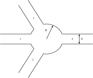
Figure 1: Three-terminal Quantum Switch

The aim of this section is: to construct a solvable model for general Quantum network with a finite number of semi-infinite wires. The model network will be constructed of a single vertex, where the essential part of the intermediate operator is substituted by some finite-dimensional operator, and several quasi-one-dimensional quantum wires attached to it, emulating the open channels. We will choose the parameters of the model such that the corresponding Scattering matrix will coincide with the essential Scattering matrix of the Quantum Network (36). Similar construction for the simplest Quantum Network - a three-terminal Quantum Switch - was developed in preprint MPP03 , see Fig.1 below. We will use in this section notations similar to ones introduced in section 2

$${U}_{{}_{{}_{\Omega}}}=\sum_{t}\oplus\,\,u_{{}_{\Omega_{t}}},\,\,{U}^{{}^{\omega}}=\sum_{{}_{t,m}}\oplus\,\,{u}^{{}^{\omega}}_{{}_{t,m}},$$

but we assume now that vector functions ${U}_{{}_{{}_{\Omega}}},\,{U}^{{}^{\omega}}$ present elements of functional spaces not on the bottom sections of channels, but on the vertex domains and wires respectively. With these notations we can present the basic Schrödinger equation on the vertex domains and on the wires in symbolic form

$$-\frac{1}{\mu_{{}_{\Omega}}}\bigtriangleup{U}_{{}_{\Omega}}+V_{{}_{\Omega}}{U}_{{}_{\Omega}}=E\,{U}_{{}_{\Omega}}$$

$$-\frac{1}{\mu^{{}^{\parallel}}}\frac{\partial^{{}^{2}}{U}^{{}^{\omega}}}{\partial x^{{}^{2}}}+\frac{1}{\mu^{{}^{\bot}}}\frac{\partial^{{}^{2}}{U}^{{}^{\omega}}}{\partial y^{{}^{2}}}+V^{{}^{\omega}}\,{U}^{{}^{\omega}}=E\,{U}^{{}^{\omega}},$$ (37)

with a bounded measurable potentials $V_{{}_{\Omega}}=\left\{V_{{}_{t}}\right\}$ on the wells and constant potentials $V^{{}^{\omega}}=\left\{V_{{}_{m}}\right\}$ on the wires. Consider the the entrance eigen-vectors $e^{{}^{m}}_{{}_{l}}$ of cross-section and corresponding orthogonal projections $p^{{}^{m}}_{{}_{l}}$ in spaces of square-integrable functions on bottom sections of the wires $\omega^{{}^{m}}$, see section 2, and form the entrance subspaces $E_{{}_{\pm}}$ for open and closed channels with corresponding projections

$$P_{{}_{\pm}}=\sum_{{}_{\pm}}\oplus p^{{}^{m}}_{{}_{l}},\,\,\mbox{dim}E_{{}_{+}}=N$$

with summation over the thresholds below and above the Fermi level $\Lambda$ respectively. For instance: we take for $E_{{}_{+}}$ the sum of all $p^{{}^{m}}_{{}_{l}}$ with indices satisfying the condition $\frac{1}{2\mu_{{}_{m}^{{}^{\bot}}}}\,\frac{\pi^{{}^{2}}l^{{}^{2}}}{\delta_{{}_{m}}^{{}^{2}}}+V_{{}_{m}}<\Lambda$ for $E_{{}_{+}}$. For values of the spectral parameter on the minimal spectral band $\left[\lambda_{{}_{min}}^{{}^{L}},\,\lambda_{{}_{max}}^{{}^{L}}\right]$ containing the Fermi level $\Lambda$, we introduce an operator-valued Wave-number ${\bf P}_{{}_{+}}$ for open channels as a positive square root from

$${\bf P}^{{}^{2}}_{{}_{+}}=\sum_{{}_{\left\{+\right\}}}\left\{\lambda-\frac{1}{2\mu_{{}_{m}^{{}^{\bot}}}}\,\frac{\pi^{{}^{2}}l^{{}^{2}}}{\delta_{{}_{m}}^{{}^{2}}}-V_{{}_{m}}\right\}p^{{}^{m}}_{{}_{l}}:=\lambda-{\bf V}^{{}^{\omega}},$$

with summation $\left\{+\right\}$ over all open channels, and the positive decrement $P_{{}_{-}}$ for closed channels:

$${\bf P}^{{}^{2}}_{{}_{-}}=\sum_{{}_{\left\{-\right\}}}\left\{\frac{1}{2\mu_{{}_{m}^{{}^{\bot}}}}\,\frac{\pi^{{}^{2}}l^{{}^{2}}}{\delta_{{}_{m}}^{{}^{2}}}+V_{{}_{m}}-\lambda\right\}p^{{}^{m}}_{{}_{l}}={\bf V}^{{}^{\omega}}-\lambda.$$

The introduced operators are connected with operators $K_{{}_{\pm}}$ from the previous section

$$K_{{}_{\pm}}=\sqrt{2\mu^{{}^{\parallel}}}{\bf P}_{{}_{\pm}}.$$

Corresponding exponential solutions of the Schrödinger equation in the wires are:

$$e^{{}^{\pm i\,K_{{}_{+}}\,x}}\,\,e,\,\,\mbox{with}\,\,e\in E_{{}_{+}}\,,\,\mbox{and}\,\,e^{{}^{\pm K_{{}_{-}}\,x}},\,\,e\,\,\mbox{with}\,\,e\in E_{{}_{-}}.$$

Depending on architecture of the Quantum Network one may construct the intermediate operator either blocking open channels in all wires, as suggested at the end of section 2, or blocking open channels only in semi-infinite wires. When constructing the solvable model of the network we also have a choice: either we present the whole network as a single star-shaped graph with a single resonance vertex, or as a joining of star-shaped graphs with resonance vertices, connected by finite quantum wires. In second case the parameters of the finite wires enter the model as explicit parameters. We guess that the second representation is more convenient for detailed engineering analysis of networks and especially for optimization of their transport properties. Nevertheless we choose now the former construction, firstly: as more elementary and, secondly: just to include in our construction non-trivial ( bent of periodic) internal finite wires. When analysis of the first construction is done, we can, at least in principle, develop analysis for the second one, with straight connecting wires, in algebraic way, based on star-shaped elements. Note that importance of star-shaped elements was noticed long ago and remains motivation of numerous recent papers, see for instance HarmerTh ; Exner03 . We prove here that the star- shaped graph with a “resonance vertex”, see our construction below, is an universal object in spectral theory of Quantum Graphs .

When chopping off the open channels in semi-infinite wires only, we obtain a self-adjoint intermediate operator $L_{{}_{\Lambda}}$ and construct the corresponding DN-map ${\cal D}{\cal N}^{{}^{\Lambda}}$ and the approximation of the Scattering matrix on the essential spectral band, (36). The corresponding Scattering Ansatz (22) in semi-infinite open channels satisfies the equation

$$-\frac{1}{\mu^{{}^{\bot}}}\,\frac{d^{{}^{2}}{U}^{{}^{\omega}}}{dx^{{}^{2}}}+{\bf V}^{{}^{\omega}}{U}^{{}^{\omega}}=\lambda\,\,{U}^{{}^{\omega}}.$$ (38)

We choose the outer (“trivial”) the part of the model - in open channels - in form of original matrix Schrödinger operator

$$l\,\,\,{U}^{{}^{\omega}}=-\frac{1}{\mu^{{}^{\bot}}}\,\frac{d^{{}^{2}}{U}^{{}^{\omega}}}{dx^{{}^{2}}}+{\bf V}^{{}^{\omega}}{U}^{{}^{\omega}}$$

in $L_{{}_{2}}(E,\,[0,\infty))$ and we will use the same Scattering Ansatz (22) in open wires as for the original problem. But the construction of the vertex part of the model will be done with a major change of the original intermediate operator.

Based on the above physical motivation we assume that only a finite number $N_{{}_{T}}$ of eigenvalues of the intermediate operator sits on the essential spectral band and no change of multiplicity of the continuous spectrum occurs. Then we will substitute the intermediate operator on the Network by some finite-dimensional positive hermitian matrix $A$ acting in an abstract space $E_{{}_{A}}$, dim$\,E_{{}_{A}}=\,N_{{}_{T}}$. The eigenvalues and normalized eigenvectors of the operator $A$ will be denoted by $k_{{}_{s}}^{{}^{2}},\,e_{{}_{s}}$ correspondingly, $\,s=1,2,\dots N_{{}_{T}}$. The eigenvalues and the boundary parameters of the model $\,\beta$, see below (43), will be defined later based on comparison of the Scattering matrix of the model with the essential Scattering matrix. The resulting operator ${\bf A}_{{}_{\beta}}$ we obtain is a simplest star-shaped model of the Quantum network with the compact part substituted by a sophisticate Quantum Dot. In our construction we follow the receipt of construction of zero-range potentials with inner structure described in Extensions ; Kurasov , see also references therein.

The corresponding model for the three-terminal Quantum Switch is used in PRB for estimation of the parameter regime of the switch.

Restrict both $l$ and $A$ to symmetric operators onto the corresponding domains: $l\to l_{{}_{0}}=l\bigg{|}_{{}_{D^{{}^{l}}_{{}_{0}}}}$ defined on functions vanishing near near $x=0$; the operator is restricted $A\to A_{{}_{0}}=A\bigg{|}_{{}_{D^{{}^{A}}_{{}_{0}}}}$ such that given subspace $N\in E_{{}_{A}}$ would play the role of deficiency subspace at the spectral point $i:N=N_{{}_{i}}$, dim $N=d$. Then dual deficiency subspace is ${N}_{-i}=\frac{A+iI}{A-iI}N$. Define the domain of the restricted operator $A_{{}_{0}}$ as $D^{{}^{A}}_{{}_{0}}=\frac{I}{A-iI}\,\,[E_{{}_{A}}\ominus N_{{}_{i}}]$ of $A_{{}_{0}}$. It is not dense, since $A$ is bounded. Nevertheless, under condition that the deficiency subspaces $N_{{}_{\pm}}=N_{{}_{\pm i}}$ do not have common elements, see for instance Krasn ; KP00 , the extension procedure for the orthogonal sum $l_{{}_{0}}\oplus A_{{}_{0}}$ can be developed with use of the symplectic formalism, see for instance Zero_range . The case dim$E_{{}_{A}}=1$ is not formally covered by the above condition, but the corresponding extension also was constructed in Shirokov79 ; Shirokov80 and the relevant formulae for the scattering matrix and scattered waves remain true.The extension of the restricted operator ${\bf A}_{{}_{0}}$ is reduced to selection of a Lagrangian plane of the sum of the corresponding boundary forms, see for instance Extensions ; KP00 , and below, see 43, where the Lagrangian plane is chose based on proper boundary condition. The same description of extensions remains valid in case dim$E_{{}_{A}}=1$. We will use this fact below, see 54.

The boundary form of the differential operator $l_{{}_{0}}^{{}^{+}}$ is obtained via standard integration by parts:

$${\cal J}_{{}_{l}}(U,\,V)=\langle l_{{}_{0}}^{{}^{+}}U,\,V\rangle-\langle U,\,l_{{}_{0}}^{{}^{+}}V\rangle=\langle U^{\prime}(0),\,V(0)\rangle-\langle U(0),\,V^{\prime}(0)\rangle,$$ (39)

where $U(0),\,V(0)\in E_{{}_{+}}$ and the derivatives are taken in positive direction.

We assume that the Hermitian operator $A:E_{{}_{A}}\to E_{{}_{A}}$, dim $E_{{}_{A}}=N_{{}_{T}}$, is defined by its spectral decomposition (on discrete spectrum)

$$A=\sum_{{}_{s}}^{{}^{N_{{}_{T}}}}k^{{}^{2}}_{{}_{s}}P_{{}_{s}},$$

where $k^{{}^{2}}_{{}_{s}}$ are positive eigenvalues and $P_{{}_{s}}$ are the corresponding spectral projections, $P_{{}_{s}}=e_{{}_{{}_{s}}}\rangle\langle e_{{}_{s}}$. Choose an ortho-normal basis in ${N}_{i}$ $\left\{f_{l}\right\}=\left\{f_{l,i}\right\},\,l=1,2,\dots,d,\,d=\dim{{N}_{i}}\leq N_{{}_{T}}$, as a set of deficiency vectors of the restricted operator $A_{0}$. Then vectors $\frac{A+iI}{A-iI}f_{l}$ form an ortho-normal basis in the dual deficiency subspace $N_{{}_{-i}}$. We assume that the subspaces ${N}_{i}$ and ${N}_{-i}$ do not overlap, hence their (direct) sum ${\cal N}={N}_{i}{+}{N}_{-i}$,- the defect of the operator $A_{{}_{0}}$, - has the dimension $2d=2$. Under this assumption the deficiency index of the restricted operator $A_{0}$ is equal to $(d,d)$. The defect contains elements from the domain $D_{0}$ of $A$, so the restricted operator $A_{0}=A\big{|}_{D_{0}}$ is not densely defined, and hence the adjoint operator does not exist. However, under the above condition one may use the formal adjoint $A_{0}^{+}$ defined on defect:

$$u=\sum_{l=1}^{d}[x_{l,i}\,e_{l,i}+x_{l,-i}\,e_{l,-i}]\,\in\,{\cal N},$$

by the von-Neumann formula, see for instance Glazman ,

$$A_{0}^{+}u=\sum_{l=1}^{d}[-i\,\,x_{l,i}\,f_{l,i}+i\,\,x_{l,-i}\,f_{l,-i}].$$

We will use the formal adjoint during the construction of extensions (see Krasn ; KP00 ) since, for closed operators with the finite deficiency indices, the construction of the extension is actually developed in the defect. In order to use the symplectic version of the operator-extension techniques we introduce in the defect ${\cal N}$ a new basis $w_{\pm,l}$, on which the formal adjoint $A_{0}^{+}$ is correctly defined due to the above assumption of non-overlapping:

$$w_{{}_{l,+}}=\frac{f_{{}_{l,i}}+f_{{}_{l,-i}}}{2}=\frac{A}{A-iI}f_{{}_{l}},\,\,w_{{}_{l,-}}=\frac{f_{{}_{l,i}}-f_{{}_{l,-i}}}{2i}=-\frac{I}{A-iI}f_{{}_{l}},$$

$$A_{0}^{+}w_{{}_{l,+}}=w_{{}_{l,-}},\,\,A_{0}^{+}w_{{}_{l,-}}=-w_{{}_{l,+}}.$$

The following formula of integration by parts with abstract operators was proved in (Zero_range ; Extensions ):

Lemma V.1

Consider elements from the domain of the (formal) adjoint operator $A_{0}^{+}:$

$$u=u_{0}+\sum_{l}[\xi^{{}^{u}}_{{}_{l,+}}w_{{}_{l,+}}+\xi^{{}^{u}}_{{}_{l,-}}w_{{}_{l,-}}]=u_{0}+\frac{A}{A-iI}\vec{\xi}^{{}^{u}}_{{}_{+}}-\frac{1}{A-iI}\vec{\xi}^{{}^{u}}_{{}_{-}},$$

$$v=v_{0}+\frac{A}{A-iI}\vec{\xi}^{{}^{v}}_{{}_{+}}-\frac{1}{A-iI}\vec{\xi}^{{}^{v}}_{{}_{-}}$$

with symplectic coordinates $\vec{\xi}^{u}_{\pm},\,\vec{\xi}^{v}_{\pm}$:

$$\vec{\xi}^{{}^{u}}_{{}_{\pm}}=\sum_{l}\xi^{{}^{u}}_{{}_{l,\pm}}f_{{}_{l,i}}\in{N},\,\,\vec{\xi}^{{}^{v}}_{{}_{\pm}}=\sum_{l}\xi^{{}^{v}}_{{}_{l,\pm}}f_{{}_{l,i}}\in{N}.$$

Then, the boundary form of the formal adjoint operator is equal to

$${\cal J}_{{}_{A}}(u,v)=\langle A_{0}^{+}u,v\rangle-\langle u,A_{0}^{+}v\rangle=\langle\vec{\xi}^{{}^{u}}_{{}_{+}},\vec{\xi}^{{}^{v}}_{{}_{-}}\rangle_{{}_{N}}-\langle\vec{\xi}^{{}^{u}}_{{}_{-}},\vec{\xi}^{{}^{v}}_{{}_{+}}\rangle_{{}_{N}}.$$ (40)

The fundamental Krein formula K ; MN for Generalized Resolvents of Symmetric Operators can be easily derived from the next statement proved inExtensions . It helps to solve the non-homogeneous equations with the adjoint operator $(A^{{}^{+}}_{{}_{0}}-\lambda I)u=f$. In our situation similar to Ad_Pav it is used in course of calculation of the scattering matrix , see below (44).

Lemma V.2

The symplectic coordinates $\vec{\xi}^{{}^{u}}_{{}_{\pm}}\in N$ of the vector-valued function

$$u=\frac{A+iI}{A-\lambda I}\,\,\,\vec{\xi}^{{}^{u}}_{{}_{+}}:=u_{0}+\frac{A}{A-iI}\vec{\xi}^{{}^{u}}_{{}_{+}}-\frac{1}{A-iI}\vec{\xi}^{{}^{u}}_{{}_{-}},$$ (41)

which satisfies the adjoint equation $[A_{0}^{+}-\lambda I]u=0$, are connected by the formula

$$\vec{\xi}^{{}^{u}}_{{}_{-}}=-P_{N}\frac{I+\lambda A}{A-\lambda}\vec{\xi}^{{}^{u}}_{{}_{+}}$$ (42)

The operator-function

$${\cal M}=P_{N}\frac{I+\lambda A}{A-\lambda I}P_{N}:{N}\to{N},$$

with a positive imaginary part in the upper half-plane $\Im\lambda>0$ coincides actually with “$Q$-function”, introduced by M. Krein (K ). It serves an abstract analog of the celebrated function used by H. Weyl in course of construction of self-adjoint extensions of the second order differential operator of Schrödinger type, see, for instance Titchmarsh , where the original construction by H.Weyl is presented. The operator-function ${\cal M}$ exists almost everywhere on real axis $\lambda$ and has a finite number of simple poles sitting at the eigenvalues $k_{{}_{l}}^{{}^{2}}$ of $A$. This function plays an important role in description of spectral properties of self-adjoint extensions of symmetric operators, see K ; Zero_range ; Gorbachuk .

The boundary form ${\bf J}({\bf U},{\bf V})$ of the orthogonal sum ${\bf A}_{0}^{+}=A_{0}^{+}\oplus{l}_{0}^{+}$ of the restricted matrix and the differential operator on elements $(U,u)={\bf U}$ on the orthogonal sum of the corresponding spaces is calculated as a sum of the forms (39,40). The self-adjoint extensions of the corresponding operator ${\bf A}_{0}=A_{0}\oplus{l}_{0}$ are obtained as restrictions of the adjoint operator ${\bf A}_{0}^{+}=A_{0}^{+}\oplus{l}_{0}^{+}$ onto Lagrangian planes of the form ${\bf J}({\bf U},{\bf V})$. These planes may be defined by the boundary conditions connecting the symplectic coordinates $U^{\prime}(0),\,U(0),\,\,\vec{\xi}^{u}_{+},\,\vec{\xi}^{u}_{-}$ of components of the corresponding elements in the deficiency subspaces. For instance, one may select a $d$-dimensional operator $\beta:E\to{\cal E}$ and define the Lagrangian plane ${\bf L}_{\beta}$ by the boundary condition

$$\left(\begin{array}[]{c}U^{\prime}(0)\\ -\vec{\xi}_{+}\end{array}\right)=\left(\begin{array}[]{cc}\beta_{{}_{00}}&\beta_{{}_{01}}\\ \beta_{{}_{01}}^{{}^{+}}&0\end{array}\right)\left(\begin{array}[]{c}U(0)\\ -\vec{\xi}_{-}\end{array}\right).$$ (43)

This condition defines a self-adjoint extension ${\bf A}_{\beta}$ of the restricted operators $A_{0}\oplus l_{0}$ in $L_{2}(R,{E_{{}_{+}}})\oplus E_{{}_{A}}$. The absolutely continuous of the operator ${\bf A}_{\beta}$ coincides with the spectrum of the exterior part of the model, hence - with the spectrum of the trivial component $l_{{}_{\Lambda}}$ of the split operator ${\cal L}_{{}_{\Lambda}}$ . The corresponding eigenfunctions of ${\bf A}_{{}_{\beta}}$ on the minimal spectral band $\lambda_{{}_{\max}}^{{}^{\Lambda}}\lambda_{{}_{min}}^{{}^{\Lambda}}$ containing the Fermi-level can be found via substitution into above boundary condition the column combined of Anzatzes (22) and (41)

$$\Psi=\left(\begin{array}[]{c}e^{-iK_{+}x}\nu+e^{iK_{+}x}{\bf S}\nu\\ \frac{A+iI}{A-\lambda I}\vec{\xi}^{u}_{+}\end{array}\right).$$

It gives the linear equation for Scattering matrix:

$$\left(\begin{array}[]{c}-iK_{{}_{+}}\left(\nu-S\nu\right)\\ -\vec{\xi}_{{}_{+}}\end{array}\right)=\left(\begin{array}[]{cc}\beta_{{}_{00}}&\beta_{{}_{01}}\\ \beta_{{}_{00}}^{{}^{+}}&0\end{array}\right)\,\,\left(\begin{array}[]{c}\nu+S\nu\\ {\cal M}\vec{\xi}_{{}_{+}}\end{array}\right).$$

Solving this equation we can obtain the Scattered waves and the formula we needed:

Lemma V.3

The Scattering matrix for the constructed model is an analytic function of the spectral parameter $\lambda$:

$${\bf S}(\lambda)=\frac{iK_{{}_{+}}+\left[\beta_{{}_{00}}-\beta_{{}_{01}}{\cal M}\beta_{{}_{10}}\right]}{iK_{{}_{+}}-\left[\beta_{{}_{00}}-\beta_{{}_{01}}{\cal M}\beta_{{}_{10}}\right]},$$ (44)

with denominator of the fraction preceding the numerator.

Now we will choose the parameter $\beta$ such that the operator-function $\left[\beta_{{}_{00}}-\beta_{{}_{01}}{\cal M}\beta_{{}_{10}}\right]$ acting in $E_{{}_{+}}$ coincides with the essential component ${\cal D}{\cal N}^{{}^{\Lambda}}_{{}_{T}}$ of the DN-map of the intermediate operator. Really, denote by $Q_{{}_{s}}$ the spectral projection onto the eigen-space of $A$ corresponding to the eigenvalue $k^{{}^{2}}_{{}_{s}}$ framed by projections onto the deficiency subspace $N_{{}_{i}}=N$

$$Q_{{}_{s}}=P_{{}_{i}}e_{{}_{s}}\rangle\langle P_{{}_{i}}e_{{}_{s}}.$$

Then the above expression takes the form :

$$\left[\beta_{{}_{00}}-\beta_{{}_{01}}{\cal M}\beta_{{}_{10}}\right]=$$

$$\left[\beta_{{}_{00}}+\sum_{{}_{s=1}}^{{}^{N_{{}_{T}}}}k_{{}_{s}}^{{}^{2}}\beta_{{}_{01}}Q_{{}_{s}}\beta_{{}_{10}}\right]+\sum_{{}_{s}}\frac{1+k_{{}_{s}}^{{}^{4}}}{k_{{}_{s}}^{{}^{2}}-\lambda}\beta_{{}_{01}}Q_{{}_{s}}\beta_{{}_{10}}.$$ (45)

We will define the boundary parameters $\beta_{{}_{10}},\,\,\beta_{{}_{01}}=\beta_{{}_{10}}^{{}^{+}}$ later, but once they are defined, we choose $\beta_{{}_{00}}$ such that the first summand in the right side of (45) vanishes: $\beta_{{}_{00}}+\sum_{{}_{s}}k_{{}_{s}}^{{}^{2}}\beta_{{}_{01}}Q_{{}_{s}}\beta_{{}_{10}}=0$. Then the Scattering matrix take the form:

$${\bf S}(k)=\frac{iK_{{}_{+}}-\sum_{{}_{s=1}}^{{}^{N_{{}_{T}}}\frac{1+k_{{}_{s}}^{{}^{4}}}{k_{{}_{s}}^{{}^{2}}-\lambda}\beta_{{}_{01}}Q_{{}_{s}}\beta_{{}_{10}}}}{iK_{{}_{+}}+\sum_{{}_{s}}\frac{1+k_{{}_{s}}^{{}^{4}}}{k_{{}_{s}}^{{}^{2}}-\lambda}\beta_{{}_{01}}Q_{{}_{s}}\beta_{{}_{10}}},$$ (46)

, which coincides with the essential Scattering matrix if and only if the corresponding Krein -function

$$\sum_{{}_{s=1}}^{{}^{N_{{}_{T}}}}\frac{1+k_{{}_{s}}^{{}^{4}}}{k_{{}_{s}}^{{}^{2}}-\lambda}\beta_{{}_{01}}Q_{{}_{s}}\beta_{{}_{10}}$$ (47)

coincides with with the essential part ${\cal D}{\cal N}^{{}^{\Lambda}}_{{}_{T}}$ of the $DN$-map of the intermediate operator - the finite sum of polar terms

$$\sum_{{}_{s=1}}^{{}^{N_{{}_{T}}}}\frac{P_{{}_{+}}\frac{\partial\varphi_{{}_{s}}}{\partial n}\rangle\langle P_{{}_{+}}\frac{\partial\varphi_{{}_{s}}}{\partial n}}{\lambda_{{}_{s}}-\lambda}.$$ (48)

Summarizing above results we obtain the following conditional statement statement for the extension constructed based on the boundary condition (43) in case when $N_{{}_{i}}\cap N_{{}_{-i}}=0$ or dim $E_{{}_{A}}=1$:

Theorem V.1

The constructed operator ${\bf A}_{{}_{\beta}}$ is a solvable model of the Quantum network on the essential interval of energy if and only if the dimension of the space $E_{{}_{A}}$ coincides with the number of eigenvalues on the essential interval of energy, the eigenvalues $k^{{}^{2}}_{{}_{s}}$ of the operator $A=\sum_{{}_{s=1}}^{{}^{N_{{}_{T}}}}k^{{}^{2}}_{{}_{s}}e_{{}_{s}}\rangle\,\langle e_{{}_{s}}$, with some ortho-normal basis $e_{{}_{s}}$, coincide with eigenvalues of the intermediate operator on essential interval of energy and there exist a subspace $N_{{}_{i}}=N$ and operator $\beta_{{}_{01}}:N_{{}_{i}}\to E_{{}_{+}}$ such that for that ortho-normal basis $\left\{e_{{}_{s}}\right\}_{{}_{s=1}}^{{}^{N_{{}_{T}}}}$ in $E_{{}_{A}}$

$$P_{{}_{+}}\frac{\partial\varphi_{{}_{s}}}{\partial n}=\beta_{{}_{01}}P_{{}_{i}}e_{{}_{s}}$$ (49)

for all $s,\,s=1,2,3,\dots,N_{{}_{T}}$.

In case when only one resonance eigen-value $k^{{}^{2}}_{{}_{0}}$ of the intermediate operator sits on the essential spectral band the obtained model Scattering matrix

$${\bf S}(p)=\frac{iK_{{}_{+}}-\frac{1+k_{{}_{0}}^{{}^{4}}}{k_{{}_{0}}^{{}^{2}}-\lambda}\beta_{{}_{01}}Q_{{}_{0}}\beta_{{}_{10}}}{iK_{{}_{+}}+\frac{1+k_{{}_{0}}^{{}^{4}}}{k_{{}_{0}}^{{}^{2}}-\lambda}\beta_{{}_{01}}Q_{{}_{0}}\beta_{{}_{10}}}$$ (50)

is a one-pole approximation of the Scattering matrix of the network. The condition of the above theorem are obviously fulfilled for one-pole approximation, when $P_{{}_{+}}\frac{\partial\varphi_{{}_{0}}}{\partial n}\neq 0$, $d=1,\,N_{{}_{T}}=1$, and $\beta_{{}_{0}}$ is one-dimensional operator mapping the one-dimensional subspace $N_{{}_{i}}$ onto the resonance entrance subspace in $E_{{}_{+}}$ spanned by $P_{{}_{+}}\frac{\partial\varphi_{{}_{0}}}{\partial n}$. For thin or shrinking networks one can estimate the deviation of the one-pole approximation from the exact Scattering matrix on the network based on material of section 3. It will be done elsewhere.

Note that there exist an intrinsic connection between the matrix model of the network we propose and method of derivation of the asymptotic of different series of eigenfunctions of Laplace operator on a composite domain with shrinking channels : both are actually based on a shape of eigenfunctions in limiting domain. We hope to develop a comparative analysis of both problems in a forthcoming publication.

The above one-pole approximation has also another important role in perturbation theory: as a sort of a “jump-start” in analytic perturbation procedure. This role may be clarified by the following observation. Consider a simplest network with only one semi-infinite wire and the Fermi level sitting on the first spectral band multiplicity $1$. Then the component of the corresponding solvable model in the open channel is presented by the Schrödinger equation

$$-u^{\prime\prime}=\lambda u:=p^{{}^{2}}u,\,\,0<x<\infty,$$

with one-dimensional entrance subspace $E_{{}_{+}}$. Construct the solvable model ${\bf A}_{{}_{\beta}}$ of the network assuming that the “inner Hamiltonian” $A$ in course of construction of the solvable model is restricted to a symmetric operator with one-dimensional deficiency subspace $N_{{}_{i}}:=N$ spanned by the vector $e$, and $\beta_{{}_{01}}:=\beta$ is the map of $N$ onto $E_{{}_{+}}$. Then the model Scattering matrix is scalar :

$${\bf S}_{\beta}(p)=\frac{ip-\beta^{{}^{2}}\sum_{{}_{s}}\frac{1+k_{{}_{s}}^{{}^{4}}}{k_{{}_{s}}^{{}^{2}}-p^{{}^{2}}}Q_{{}_{s}}}{ip+\beta^{{}^{2}}\sum_{{}_{s}}\frac{1+k_{{}_{s}}^{{}^{4}}}{k_{{}_{s}}^{{}^{2}}-p^{{}^{2}}}Q_{{}_{s}}}$$ (51)

with $Q_{{}_{s}}=|\langle e,e_{{}_{s}}\rangle|^{{}^{2}}$. Zeroes $k_{{}_{s}}(\beta)$ of the Scattering matrix (51) - resonances - sit in upper half-plane and approach the points $\pm k_{{}_{s}},\,k_{{}_{-s}}=-k_{{}_{s}}$, when $\beta\to 0$. They can be found approximately in form of branching continuous fractions, see Voevodin as solutions of a chain of algebraic equations. For instance the resonance $p_{{}_{0}}=k_{{}_{0}}(\beta)$ created from the eigenvalue $k^{{}^{2}}_{{}_{0}}$ of the operator $A$ ( more precise : from the point $+k_{{}_{0}}$ ) can be obtained as a solution $p=k_{{}_{0}}(\beta)$ of the equation

$$p=k_{{}_{0}}-\frac{\beta^{{}^{2}}(1+k^{{}^{4}}_{{}_{0}})Q_{{}_{0}}}{(p+k_{{}_{0}})\left(ip-\beta^{{}^{2}}\sum_{{}_{s\neq 0}}\frac{1+k_{{}_{s}}^{{}^{2}}}{k_{{}_{s}}^{{}^{2}}-p^{{}^{2}}}Q_{{}_{s}}\right)}.$$ (52)

Another resonance created at the point $-k_{{}_{0}}$ from the eigenvalue $k^{{}^{2}}_{{}_{0}}$ sits at the symmetric point $-\bar{k}_{{}_{0}}(\beta)$ with respect to the imaginary axis. Other resonances $k_{{}_{s}}(\beta)$ can be found from similar equations with $\pm k_{{}_{0}}$ substituted by $\pm k_{{}_{s}}$. All functions $k_{{}_{s}}(\beta)$ are analytic functions of $\beta,\,k$ in small neighborhoods of $(0,\,\pm k_{s})$. They sit in the upper half-plane symmetrically with respect to the imaginary axis $k_{{}_{-s}}(\beta)=-\bar{k}_{{}_{s}}(\beta)$. The Scattering matrix (51) is unitary on the real axis $k$ and has poles at the complex-conjugate points $\bar{k}_{{}_{s}}(\beta)$ in the lower half-plane , hence it is presented by the finite Blashke product which tends to $1$ when $|k|\to\infty$:

$${\bf S}^{{}^{\beta}}(p)=\prod_{s}\frac{p-k_{{}_{s}}(\beta)}{p-\bar{k}_{{}_{s}}(\beta)}.$$ (53)

The outer component of the scattered wave is presented as

$$\Psi^{{}^{\beta}}_{{}_{0}}=e^{-ipx}+{\bf S}^{{}^{\beta}}(k)e^{-ipx},$$

and fulfills proper boundary condition at the place of contact with the model quantum dot.

Though the resonances depend analytically of $(\beta,\,p\,)$, neither Scattering matrix (51) nor the Scattered wave depend analytically of $\left(\beta,p\right)$ on the product $(U_{{\beta}},C_{{}_{p}})$ of a small neighborhood of the origin in $\beta$ - plane and the whole $p$-plane. The analyticity is lost due to presence of points $\pm k_{{}_{s}}$ where the resonances are created at the origin of the $\beta$-plane. But it is present for “separated” factors of the Scattering Matrix. Consider for small $\beta$ two non intersecting subsets $K_{{}_{0}}$ and $K^{{}^{0}}$ of the set $K=\left\{k_{s}\right\}$ and the corresponding factors ${\bf S}^{{}^{\beta}}_{{}_{0}},\,{\bf S}_{{}_{\beta}}^{{}^{0}}$ of the Scattering matrix with resonances created in $K_{{}_{0}},\,K^{{}^{0}}$ respectively:

$${\bf S}^{{}^{\beta}}_{{}_{0}}(p)=\prod_{{}_{k_{{}_{s}}\in K_{{}_{0}}}}\frac{p-k_{{}_{s}}}{p-\bar{k}_{{}_{s}}},\,\,\,\,\,{\bf S}_{{}_{\beta}}^{{}^{0}}(p)=\prod_{{}_{k_{{}_{s}}\in K^{{}^{0}}}}\frac{p-k_{{}_{s}}}{p-\bar{k}_{{}_{s}}}.$$

Here the first factor is an analytic function of $(\beta,\,p)$ when $\beta$ is small and $p$ sits near $K^{{}^{0}}$, and , vice versa, the second factor is analytic for small $\beta$ and $p$ sits in a small neighborhood of $K_{{}_{0}}$. In particular the first factor can be expand into Taylor series in $(\beta,\,p)$ for small $\beta\in U_{{\beta}}$ if $p$ sits in some small neighborhood $U^{{}^{0}}$ of $K^{{}^{0}}$, and the second factor is presented by the Taylor series in $(\beta,\,p)$ if $\beta\in U_{{\beta}}$ and $p$ sits in a small neighborhood $U_{{}_{0}}$ of $K_{{}_{0}}$. On the other hand, the first factor is not an analytic function of $(\beta,\,p)$ if $\beta\in U_{{}_{\beta}}$ and $p$ is near to $K_{{}_{0}}$. This observation may be interpreted as a fact of the perturbation theory the following way.

Assume that $k_{{}_{0}}>0$ and consider the representation of the Scattering matrix (53) in form of product of two factors : the product containing the resonances $k_{{}_{0}}(\beta),\,-\bar{k}_{{}_{0}}(\beta)$ created from the eigenvalue $k^{{}^{2}}_{{}_{0}}$

$${\bf S}^{{}^{\beta}}_{{}_{0}}(p)=\frac{[p-k_{{}_{0}}(\beta)]\,[p+\bar{k}_{{}_{0}}(\beta)]}{[p-\bar{k}_{{}_{0}}(\beta)]\,[p+k_{{}_{0}}(\beta)]},$$

and the complementary factor ${\bf S}^{{}^{\beta}}_{{}_{0}}$

$${\bf S}_{{}_{\beta}}^{{}^{0}}(p)=\prod_{s\neq 0}\frac{p-k_{{}_{s}}(\beta)}{p-\bar{k}_{{}_{s}}(\beta)}.$$

One can derive from the above dispersion equation (52) that the resonances are analytic functions of the perturbation parameter $\beta$ near the origin $\beta=0$, but the factor ${\bf S}^{{}^{\beta}}_{{}_{0}}(p)$ is not for the reason discussed above.

Theorem V.2

There exist a one-dimensional perturbation ${\cal L}^{{}^{\beta}}_{{}_{0}}$ of the operator

$$l_{{}_{0}}u=-u^{\prime\prime},\,\,u\bigg{|}_{{}_{0}}=0$$

with a non-trivial inner component, such that the scattering matrix of the pair $({\cal L}^{{}^{\beta}}_{{}_{0}},\,l_{{}_{0}})$ coincides with $-{\bf S}^{{}^{\beta}}_{{}_{0}}(p)$. Then the Scattering matrix ${\bf S}$ of the complementary pair $({\cal L}^{{}^{\beta}}_{{}_{0}},\,\,{\cal L}^{{}^{\beta}})$ is equal to the complementary factor $-{\bf S}_{{}_{\beta}}^{{}^{0}}(p)$:

$${\bf S}_{{}_{\beta}}(p)={\bf S}^{{}^{\beta}}_{{}_{0}}(p)\,\,{\bf S}_{{}_{\beta}}^{{}^{0}}(p).$$

The complementary factor is an analytic function of $(\beta,\,k)$ on the product of a small neighborhood of the origin in $\beta$-plane and a small neighborhood $K_{{}_{0}}$ of $(k_{{}_{0}},\,-k_{{}_{0}})$ in $p$-plane.

Proof   Consider the one-dimensional operator $A$ with a positive eigenvalue $\kappa^{{}^{2}}$. We associate with it the Krein function ${\cal M}=\frac{1-\kappa^{{}^{2}}\,\lambda}{\kappa^{{}^{2}}-\lambda}$. Then restrict the operator $l_{{}_{0}}$ onto smooth functions vanishing at the origin $x=0$, and construct the self-adjoint extension ${\bf A}^{{}^{\beta}}_{{}_{0}}$ defined by the hermitian matrix $\left\{{\bf{\beta}}\right\}$ which connects the boundary values $\xi_{{}_{+}},\,-{\cal M}\xi_{{}_{+}}$ in $E_{{}_{A}}$ with boundary values $\Psi(0),\,\Psi^{\prime}(0)$ in $E_{{}_{+}}$:

$$\left(\begin{array}[]{c}\Psi^{\prime}\\ -\xi_{{}_{+}}\end{array}\right)=\left(\begin{array}[]{cc}\beta_{{}_{00}}&\beta_{{}_{01}}\\ \beta_{{}_{10}}&\beta_{{}_{11}}\end{array}\right)\,\,\left(\begin{array}[]{c}\Psi\\ -\xi_{{}_{-}}\end{array}\right).$$ (54)

Substituting into the above equation the corresponding Ansatz for the wave-function in the outer space

$$\Psi^{{}^{\beta}}_{{}_{0}}(x,p)=e^{-ipx}+{\bf S}^{{}^{\beta}}(p)e^{-ipx},$$

we obtain an explicit expression for the corresponding Scattering matrix ${\bf S}$ in terms of the inner Krein-function ${\cal M}(\lambda)=\frac{1+\kappa^{{}^{4}}\lambda}{\kappa^{{}^{2}}-\lambda}$ and the boundary parameters:

$${\bf S}(\lambda)=\frac{ip+\left[\beta_{{}_{00}}-\frac{|\beta_{{}_{01}}|^{{}^{2}}{\cal M}}{1+\beta_{{}_{11}}{\cal M}}\right]}{ip-\left[\beta_{{}_{00}}-\frac{|\beta_{{}_{01}}|^{{}^{2}}{\cal M}}{1+\beta_{{}_{11}}{\cal M}}\right]}.$$

Select the parameter $\beta_{{}_{11}}$ such that $1-\beta_{{}_{11}}\kappa^{{}^{2}}=0,$ then $1+\beta_{{}_{11}}{\cal M}=\beta_{{}_{11}}\frac{1+\kappa^{{}^{4}}}{\kappa^{{}^{2}}-\lambda}$, and the Scattering matrix takes the form with $\lambda=p^{{}^{2}}$

$${\bf S}(\lambda)=\frac{ip+\beta_{{}_{00}}-\frac{|\beta_{{}_{01}}|^{{}^{2}}}{\beta_{{}_{11}}(1+\kappa^{{}^{4}})}-\frac{|\beta_{{}_{01}}|^{{}^{2}}\kappa^{{}^{2}}}{(1+\kappa^{{}^{4}})\beta_{{}_{11}}}p^{{}^{2}}}{ip-\beta_{{}_{00}}+\frac{|\beta_{{}_{01}}|^{{}^{2}}}{\beta_{{}_{11}}(1+\kappa^{{}^{4}})}+\frac{|\beta_{{}_{01}}|^{{}^{2}}\kappa^{{}^{2}}}{(1+\kappa^{{}^{4}})\beta_{{}_{11}}}p^{{}^{2}}}$$

Comparing this expression with

$$-{\bf S}^{{}^{\beta}}_{{}_{0}}(p)=-\frac{[(p-k_{{}_{0}}(\beta)]\,[p+\bar{k}_{{}_{0}}(\beta)]}{[p-\bar{k}_{{}_{0}}(\beta)]\,[p+k_{{}_{0}}(\beta)]}=$$

$$\frac{-p^{{}^{2}}+2i{\Im k}_{{}_{0}}(\beta)p+|k_{{}_{0}}(\beta)|^{{}^{2}}}{p^{{}^{2}}-2i{\Im k}_{{}_{0}}(\beta)p-|k_{{}_{0}}(\beta)|^{{}^{2}}}={\bf S}(\lambda),$$

we obtain the equations for selection of parameters of the extension ${\bf A}^{{}^{\beta}}_{{}_{0}}$:

$$\frac{\beta_{{}_{00}}-\frac{|\beta_{{}_{01}}|^{{}^{2}}}{\beta_{{}_{11}}(1+\kappa^{{}^{4}})}}{|k{{}_{0}}(\beta)|^{{}^{2}}}=\frac{1}{2\Im k_{{}_{{}_{0}}}(\beta)}=\frac{|\beta_{{}_{01}}|^{{}^{2}}\kappa^{{}^{2}}}{(1+\kappa^{{}^{4}})\beta_{{}^{11}}}.$$ (55)

Solution is not unique, but may be parametrized by the functional parameter $\beta_{{}_{00}}$ :

$$\kappa^{{}^{2}}=\frac{1}{2\beta_{{}_{00}}\Im k_{{}_{0}}(\beta)-|k_{{}_{0}}(\beta)|^{2}}.$$

In particular we may choose: $\beta_{{}_{00}}=|k_{{}_{0}}(\beta)|^{2}\left(\Im k_{{}_{0}}(\beta)\right)^{{}^{-1}}$. Then

$$\kappa^{{}^{2}}=\frac{1}{|k_{{}_{0}}(\beta)|^{2}}.$$

To finalize the calculation we notice that both $|k_{{}_{0}}(\beta)|^{2}$ and $\Im k_{{}_{0}}(\beta)$ are real analytic functions of $\beta$, hence $\kappa^{2}$ is an analytic function of $\beta$. The boundary parameter $\beta_{{}_{00}}$ has a pole at the origin since $k_{{}_{0}}(\beta)\to k_{{}_{0}}(0)=\bar{k}_{{}_{0}}(0)$ when $\beta\to 0$. Other boundary parameters may be also chosen based on above equations (55) as $\beta_{{}_{11}}=|k_{{}_{0}}|^{{}^{2}},\,\,|\beta_{{}_{01}}|^{{}^{2}}=\frac{4+|k_{{}_{0}}|^{{}^{4}}}{4\Im k_{{}_{0}}}$. Alternative choice is $\kappa^{{}^{2}}=|k_{{}_{0}}|^{{}^{2}},\,\,\beta_{{}_{00}}=\frac{1+|k_{{}_{0}}|^{{}^{4}}}{2\Im k_{{}_{0}}\,|k_{{}_{0}}|^{{}^{2}}},\,|\beta_{{}_{01}}|^{{}^{2}}=\frac{1+|k_{{}_{0}}|^{{}^{4}}}{2\Im k_{{}_{0}}\,|k_{{}_{0}}|^{{}^{4}}},\,\,\beta_{{}_{11}}=|k_{{}_{0}}|^{{}^{-}2}$, with $k_{{}_{0}}:=k_{{}_{0}}(\beta)$. This accomplishes the construction of the operator ${\bf A}^{{}^{\beta}}_{{}_{0}}$.

The operator ${\bf A}^{{}^{\beta}}_{{}_{0}}$ permits to make a sort of a “jump-start” in perturbation procedure for the pair of operators $\left\{\left(l\oplus H\right),\,{\bf A}_{{}_{\beta}}\right\}$: the scattering matrix ${\bf S}^{{}^{\beta}}_{{}_{0}}(k)$ for the pair $\left\{\left(l\oplus H\right),\,{\bf A}^{{}^{\beta}}_{{}_{0}}\right\}$ is calculated in explicit form, and the complementary scattering matrix for the pair $\left\{{\bf A}^{{}^{\beta}}_{{}_{0}},\,{\bf A}_{{}_{\beta}}\right\}$, which coincides with ${\bf S}_{{}_{\beta}}^{{}^{0}}$, is an analytic function of $(\beta,\,p)$ near to the resonance $k_{{}_{0}}$ and can be calculated via standard analytical perturbation procedure.

Though the “jump-start” can help to develop the analytic perturbation procedure, according to the preceding result, but exact calculation of the pole $k_{{}_{0}}(\beta)$ and corresponding projection for the perturbed operator ${\bf A}_{{}_{\beta}}$, which were used in course of construction of the “jump-start”, may be a tricky analytical problem, comparable with the original spectral problem. On the other hand, the asymptotic expansion for these data for small $\beta$ may be useful for obtaining estimates, but does not help to derive analyticity of the complementary factor of the Scattering matrix constructed for the corresponding approximate “jump start” factor, constructed based on approximate asymptotic data.

VI Conclusion: intermediate operator in analytic perturbation techniques

Classical analytic perturbation techniques, see for instance Kato , is developed for additive perturbations of operators with discrete spectrum $A\longrightarrow A+\varepsilon B$. For perturbation of the continuous spectrum Kato suggested another techniques based on Wave operators. Detailed study of the perturbation of operators with continuous spectrum in model situations, especially for the Friedrichs model, see Friedrichs , was done in numerous mathematical papers and books, see simon and the references therein and also F64 ; PP70 ; FP84 ; H86 . It was already clear for specialists long ago, that the classical techniques of the analytic perturbation theory does not work generally on continuous spectrum (actually it works below the threshold of creation of resonances, see Friedrichs ). Probably I. Prigogine alone insisted on modification of the analytic perturbation techniques to cover the case of continuous spectrum.

According to evidence from long-time Prigogine’s collaborator Professor I. Antoniou, I.Prigogine attempted also to use the idea of an intermediate operator as a base for development of the analytic perturbation techniques for operators with continuous spectrum. He tried to construct the intermediate operator $A_{{}_{1}}$ as a function of the non-perturbed operator A with a hope that after the first step $A\to A_{{}_{1}}$ the analytical perturbation procedure for the perturbed operator $A+\varepsilon V$ presented as $A_{{}_{1}}+\varepsilon V^{\prime}$ becomes convergent. This simplest suggestion appeared to be not so efficient as expected, and Prigogine abandoned this idea finally, see Prig72 ; Prig73 ; Prig85 ; Antoniou ; Prig89 ; Prig95

Note that actually the idea of the intermediate operator in another context appeared in Splitting Method invented by I. Glazman, see Glazman . This method radically transformed in seventies the whole picture of the qualitative spectral analysis of singular differential operators, but was never used in context of the analytic perturbation procedure.

We actually suggested revisiting the idea of the intermediate operator again in a special case of quantum networks where the candidate for the role of an intermediate operator is almost obvious. In our case it is not a function of the non-perturbed operators, but is obtained from it just by a finite-dimensional perturbation. Actually we succeeded to apply the splitting method to Quantum Networks because of the step-wise structure of the continuous spectrum in wave-guides. This minor change of the original idea of Prigogine appears to be useful for perturbation problems in wave-guides. In our case the idea of the intermediate operator is automatically combined with resonances, which was anticipated long ago by Poincare and intensely discussed by Prigogine with references to Poincare, see Prig89 ; Poincare .

The only essential, and even decisive difference of our version of the intermediate operator from the version which I. Prigogine attempted to use, is the natural principle of spectral locality we impose: we construct the intermediate operator and the scattered waves via the special perturbation procedure locally- in a certain spectral interval, - but not globally, as Prigogine planned. It is quite easy to define this interval mathematically for the Quantum Networks: it is the maximal interval containing the Fermi level, Madelung , where the spectral multiplicity $n$ is constant and the scattering matrix is a square matrix size $n\times n$. This interval may be either a spectral band corresponding to some channel in one of semi-infinite wires, of a sum of several spectral bands (sort of a ”spectral terrace”) corresponding to different wires, with properly hybridized scattered waves. The structure of the corresponding scattered waves within this spectral interval is manifested by the structure of the scattering matrix and corresponds to the n-dimensional input-output. The structure of scattered waves on the neighboring spectral bands is different.

It is worth to notice, that slightly modified procedure permits to construct an hierarchy of intermediate operators also for some operators with absolutely-continuous spectrum of constant multiplicity, in particular for Friedrichs model.

In actual paper we discussed simplest wave-guiding systems composed of straight wave-guides (quantum wires). The convenience of this trivial environment appears from existence of explicit formulae for oscillatory modes in straight wave-guides: the system of thresholds and the structure of the entrance sub-spaces in this environment is trivial. Study of more interesting systems of periodic or asymptotically straight wave-guides with rapidly decreasing curvature requires a combination of our methods with Lippmann-Schwinger techniques developed in case of wave-guides with non-trivial geometry for discrete and especially for continuous spectrum, see Twisted ; Duclos ; percylind ; Krej_03 ; Krej6_03 ; Krej7_03 .

On the other hand, the suggestion to recover resonances from the discrete spectrum of some intermediate operator can be easily applied to any wave-guiding problem in trivial environment, with linear vertices, on a reasonable price of preliminary study of the “intermediate” dynamics. In particular, it permits to suggest alternative approach to study of trapped modes in acoustics and hydro-dynamics, investigated in Evans ; Davies , as well as to classical theory of electro-magnetic wave-guides with local variation of curvature, DES . An important advantage of our techniques is: the possibility of “fitting” of the constructed “solvable model” based of results of straightforward computing for the intermediate problem.

VII Acknowledgement

Two of co-authors (A.M and B.P) acknowledge support from the Russian Academy of Sciences, Grant RFBR 03-01- 00090 and from research allocation of the University of Auckland. All authors are grateful to Doctors M. Harmer, V. Olejnik and V. Kruglov for interesting comments on the text and to Dr. R. Shterenberg for extended discussion of questions concerning the singular spectrum in channels, important references and materials KNP supplied. The authors are grateful to Professor I. Antoniou for inspiring information on Prigogine’s experience in analytic perturbation theory and interesting materials supplied.

BP is grateful to Professor L. Faddeev for an extended discussion of the perturbation of the continuous spectrum for the Friedrichs model, which clarified the structure of the hierarchy of intermediate operators.

References

• (1) V. Adamyan. Scattering matrices for microschemes.Operator Theory: Adv. and Appl. 59 (1992) pp 1-10.
• (2) V.M.Adamyan,B.S.Pavlov Zero- radius potentials and M.G.Krein’s formula for generalized resolvents , Zap. Nauch. Sem. Leningrad. Otdel. Mat. Inst. Steklov. (LOMI), 149 (1986), Issled. Linein. Teor. Functsii. XV, 7-23, 186.
• (3) J. del Alamo,  C. Eugster Quantum field-effect directional coupler Appl. Phys. Letters 56 (1),  January 1, 1990, pp 78-83.
• (4) S. Albeverio, F. Gesztesy, R. Hoegh-Krohn, H. Holden, Solvable models in quantum mechanics. Springer-Verlag, New York,1988.
• (5) I. Antoniou, S. Tasaki Generalized Spectral Decompisitions of Mixing Dynamical Systems IN: International Journal of Quantum Chemistry,40 (1993), pp 425-474.
• (6) S.Albeverio, P.Kurasov Singular Perturbations of Differential Operators, London Math. Society Lecture Note Series 271. Cambridge University Press 2000, 429 p.
• (7) N.T. Bagraev, V.K. Ivanov, L.E. Kljachkin, A.M. Maljarenko, S.A. Rykov, I.A. Shelyh Interferention of charge carriers in one-dimensional semiconductor rings. Physics and techniques of semiconductors, v34 (2000) p 7.
• (8) N.T. Bagraev, V.K. Ivanov, L.E. Kljachkin, A.M. Malyarenko, I.A. Shelych. Ballistic Conductance of a Quantum Wire at finite Temperatures Semiconductors , 34, 6 (2000) p 712-716.
• (9) N.T.Bagraev, A.B.Mikhailova, B.S.Pavlov, L.V. Prokhorov, A.M.Yafyasov Temperature stability of the triadic resonance quatum switch,10-th MEL-ARI/NID Workshop, Helsinki,1-3 July 2002 Academy of Finland.
• (10) N.Bagraev,A.Mikhailova,B. Pavlov,L.Prokhorov, A.Yafyasov Resonance Quantum Switch: search of working parameters. Submitted to Phys.Rev. B.
• (11) N. Bagraev,B.Pavlov, A.Yafyasov Resonance Quantum Switch: search of working parametersIn: Internacional Conference on Simulation of Semiconductor Processes and Devices: SISPAD 2003, (Boston 3-5 Sept.2003),pp 275-278
• (12) C.W.J.Beenakker, H. van Houten. Quantum transport in semiconductor nanostructures. In: H.Ehrenreich, D.Turnbull (Eds.) Solid State Physics. Advances in Research and Applications. 44 (1991). Academic Press, San Diego. p. 1-228.
• (13) F.A.Berezin, L.D. Faddeev A remark on Schrödinger equation with a singular potential Soviet Math. Dokl. 2 (1961) pp 372-376
• (14) V. Bogevolnov, A, Mikhailova, B. Pavlov, A. Yafyasov About Scattering on the Ring In: ”Operator Theory : Advances and Applications”, Vol 124 (Israel Gohberg Anniversary Volume), Ed. A. Dijksma, A.M. Kashoek, A.C.M.Ran, Birkhäuser, Basel 2001,pp 155-187.
• (15) M.Büttiker, A.Pretre, H.Thomas Dynamic conductance and the scattering Matrix of Small Conductors Phys. Rev. Lett. 70 (1993) pp 4114-4117
• (16) M.Büttiker,Y.Imry,R.Landauer,S.Pinhas, Generalized many-channel conductance formula with application to small rings Phys.Rew.B 31 (1985), pp 6207-6215
• (17) R.Carlson Adjoint and self-adjoint differential operators on graphs Electron. J. Differential Equations 1998, No. 6, 10 pp. (electronic).
• (18) E.B. Davies and L. Parnovski Trapped modes in acoustic waveguides Quart. Journal Mech. ASppl. Math. 51 (1998) pp 477-492
• (19) Y.Dermenjian, M. Durand, and V. Iftimie Spectral analysis of an acoustic multistratified perturbed cylinder Commun. in Partial Differential Equations 23, 1&2, (1998) pp 141-169
• (20) P.Duclos, P. Exner and P. Stovicek Curvature-induced resonances in two-dimensional Dirichlet tube Ann. Inst. H. Poincare 62 (1995), pp 81-101
• (21) P.Duclos, P. Exner, D. Krejcirik Bound states in curved quantum layers Commun. Math. Physics 223 (2001) pp 13-28
• (22) European Comission IST programme: Future and emerging Technologies. Technology Roadmap for Nanoelectronics, R. Compano (ed.), Second edition, Nov. 2000. Luxemburg: Office for Official Publications of the European Communities. 105 p.
• (23) M.S.P. Eastham, H. Kalf Schrödinger type operators with continuous spectra Research Notes in Mathematics, 65 Pitman (Advanced Publishing Program), Boston, Mass.- London (1982) 281 pp.
• (24) J.Edward Eigenfunction decay and eigenvalues accumulation for the laplacian on asymptotically perturbed waveguides In: Journal of London Mathematical Society,59, 2 (1999), pp 177-182
• (25) D.Evans, L. Levitin and D. Vassiliev Existence theorems for trapped modes Journ. Fluid Mech. 261 (1994) pp 21-31
• (26) P. Exner, K. Nemcova Leaky Quantum Graphs: approximation by Point Interaction Hamiltonians J. Phys. A, 36 (2003) 10173 - 10193
• (27) P. Exner, P. Ŝeba. A new type of quantum interference transistor. Phys. Lett. A 129:8,9 (1988) pp 477-480.
• (28) P. Exner, P. Ŝeba , M.Tater Bound states and Scattering in quantum waveguides coupled laterally through a boundary window Journal of Mathematical Physics, 37 (1996), 10 , pp 4467-4887.
• (29) K.O.Friedrichs On the perturbation of continuous spectra Communications in Pure and Applied Mathematics 1 (1948) pp 361-406.
• (30) L.Faddeev On a model of Friedrichs in the theory of perturbations of the continuous spectrum Trudy Mat. Inst. Steklov 73 (1964) pp 292-313.
• (31) L.Faddeev,B.Pavlov Zero-sets of operator-functions with a positive imaginary part In: Linear and Complex Analysis Problems (199 Research Problems ) Lecture Notes in Mathematics 1043, ed. V. Havin, S. Hruschev, N. Nikolskii (1984) pp 124-128.
• (32) M. Faddeev, B. Pavlov. Scattering by resonator with the small openning. Proc. LOMI, v126 (1983). (English Translation J. of Sov. Math. v27 (1984) pp 2527-2533)
• (33) N.I. Gerasimenko and B.S. Pavlov. Scattering problems on compact graphs. Theor. Math. Phys. 74, 230 (1988).
• (34) Y.Ginzburg Multiplicative representations and minorants of bounded analytic operator-functions In: Functional Analysis and it’s Applications, 1:3 (1967),pp 9-23
• (35) I. Glazman Direct methods of qualitative spectral analysis of singular differential operators Translated from the Russian by the IPST staff (Israel Program for Scientific Translations), Jerusalem, 1965; Daniel Davey & Co., Inc., New York 1966 , 234 p.
• (36) I.S. Gohberg and E.I. Sigal. Operator extension of the theorem about logarithmic residue and Rouchet theorem. Mat. Sbornik. 84 (1971) p 607.
• (37) J. Goldstone and R.L. Jaffe Bound states in twisting tubes Phys. Rev. B 45 (1992) 14100-14107
• (38) V.I.Gorbachuk Boundary problems for differential- operator equations (in Russian) Kiev, Naukova Dumka (1984) 284 p
• (39) M. Harmer The matrix Schr dinger operator and the Schr dinger operator on graphs PhD thesis, Auckland University, 2000.
• (40) M. Harmer Inverse scattering for the matrix Schr dinger operator and Schr dinger operator on graphs with general self-adjoint boundary conditions ANZIAM Journal, 43 (2002), 1-8.
• (41) J.Howland. Finite rank perturbations of singular spectra Proc. Amer. Math. Soc. 97 (1986), no. 4, pp 634–636.
• (42) H.Ishio,K.Nakamura Quantum Transport in Open Billiards: Dependence on Degree of Opening J.Phys. Society Japan 61 (1992) pp 2649-2651
• (43) S. Jimbo Perturbation formula of eigenvalues in a singularly perturbed domain J. Math. Soc. Japan 45, 2 (1993), pp 340-356
• (44) V. Kalvin, P. Nejtaanmjaki,B.Plamenevskij On accumulations of the discrete spectrum of elliptic boundary problems in domains with cylindrical tails. Manuscript.
• (45) H. Kasai,K. Mitsutake, A. Okiji Effects of Confining Geometry on Ballistic Transport in Quantum Wires J.Phys. Society Japan60 (1991) pp 1679-1688
• (46) T. Kato Perturbation theory for linear operators Springer Verlag, Berlin-Heidelberg-NY, Second edition, 740 pp.
• (47) V.Kondratjev, E.Landis Qualitative theory of second order linear partial differential equations in: Partial adifferential Equations 3, ITOGI NAUKI SSSR, VINITI, Moscow (1988) pp 99-215.
• (48) A.Silbergleit, Yu. Kopilevich Spectral theory of guided waves. Institute of Physics publishing, Bristol (1996), 310 p.
• (49) D. Krejcirik Quantum strips of surfaces J. Geom. Phys. 45, 1-2 (2003) pp 203-217
• (50) D. Krejcirik and J. Kriz On the spectrum of curved Quantum Waveguides arXiv:math-ph/0306008 v1 3 June 2003, 34 p.
• (51) David Krejcirik and Rafael Tiedra de Aldecoa The nature of the essential spectrum in curved quantum waveguides arXiv: math-ph/ 0307019 v1 9 July 2003, 20 p.
• (52) V. Kostrykin and R. Schrader. Kirchhoff’s rule for quantum wires. J. Phys. A: Math. Gen. v32 (1999) pp 595-630.
• (53) M.A.Krasnosel’skij On selfadjoint extensions of Hermitian Operators(in Russian) Ukrainskij Mat.Journal 1(1949) pp 21-38
• (54) M.Krein Concerning the resolvents of an Hermitian operator with deficiency index (m,m),Doklady AN USSR ,52 (1946) pp 651-654.
• (55) P. Kuchment, H. Zengh Convergence of spectra of mesoscopic systems collapsing onto graph Journal Math. Anal. Appl. 258 (2001), pp 671-700
• (56) P. Kuchment Graph models for waves in thin structures Waves in Periodic and Random Media, 12 (2002) pp 1-24.
• (57) P. Kurasov,  B. Pavlov,Operator relation and Scattering matrix In: Operator Theory: Advances and Applications, 113, ed. Nikolskij and all, Complex Analysis, Operators and Related Topics, S.A.Vinogradov - in memoriam, Birkhauser Verlag, Basel,2000, pp 294-305.
• (58) R.Landauer Electrical Resistance of Disordered One-dimensional Lattices Phil. Mag. 21(1970) pp 863-867
• (59) P. Lax, R. Phillips Scattering theory Academic press,New York,1967.
• (60) O. Madelung. Introduction to solid-state theory. Translated from German by B. C. Taylor. Springer Series in Solid-State Sciences, 2. Springer-Verlag, Berlin, New York, 1978. 486 p.
• (61) V. M. Maz’ja. Sobolev Spaces, Translated from the Russian by T. O. Shaposhnikova. Springer Series in Soviet Mathematics. Springer-Verlag, Berlin (1985).
• (62) A. Mikhailova, B. Pavlov, I. Popov, T. Rudakova, A. Yafyasov Scattering on Compact Domain with Few Semi-Infinite Wires Attached: resonance case In: ” Mathematishe Nachrichten”, 235,1 (2002) ,pp 101 -128.
• (63) A.Mikhailova, B. Pavlov Quantum Domain as a triadic Relay In: Unconventional models of Computations UMC’2K, ed. I. Antoniou, C. Calude, M.J. Dinneeen, Springer Verlag series for Discrete Mathematics and Theoretical Computer Science (2001) pp 167-186
• (64) A.Mikhailova, B. Pavlov, L. Prokhorov Modelling of Quantum Networks, Department of Mathematics of the University of Auckland report series, 508, October 2003, 49 p.
• (65) M.Naimark Self-adjoint extensions of the second kind of a symmetric operatots, Bull.AN USSR, Ser.Math.4 (1946), pp 53-104.
• (66) S.P. Novikov.Schrödinger operators on graphs and symplectic geometry, in: The Arnol’dfest (Proceedings of the Fields Institute Conference in Honour of the 60th Birthday of Vladimir I. Arnol’d), eds. E. Bierstone, B. Khesin, A. Khovanskii, and J. Marsden, Fields Institute Communications Series, 1999.
• (67) T.Palm, L.Thylen Analysis of an of an electron-wave Y-branch switch Applied Phys. Letters 60 (1992) pp 237-239
• (68) B.Pavlov. S-Matrix and Dirichlet-to-Neumann Operators In: Scattering (Encyclopedia of Scattering), ed. R. Pike, P. Sabatier, Academic Press, Harcourt Science and Tech. Company (2001) pp 1678-1688
• (69) B.Pavlov Resonance Quantum Switch: matching domains In: Surveys in Analysis and Operator Theory.Proc. of the Center of Math. and Appl. ANU 40 Nov. 2002, pp 127-156
• (70) B. Pavlov. The theory of extensions and explicitly solvable models (In Russian) Uspekhi Mat. Nauk, 42 (1987) pp 99–131.
• (71) B.Pavlov, S.Petras The singular spectrum of a weakly perturbed multiplication operator In: Funkcional. Anal. i Priložen.(Russian) 4 no. 2, (1970) pp 54–61.
• (72) B. Pavlov A model of zero-range potential with an internal structure(in Russian) Teor. Mat. Fizika,59 (1984), pp 345-353 (English Translation : Theor. and Math. Physics 59 (1984) pp 544-550)
• (73) L. Parnovski Spetral asymptotics of the Laplace operator on manifolds with cylindrical ends In : Intern. Journ. Mathematics 6 (1995) pp 911-920
• (74) H. Poincare Methodes nouvelles de la mechanique celeste Vol. 1 (1892), Dover, New York (1957)
• (75) V.Potapov Factorization of analytic matrix-function (In Russian) Trudy Moskovskogo Matematicheskogo obschestva, 1952.
• (76) I. Prigogine, C. George, L. Rosenfeld A Unified Formulation of Dynamics and Thermodynamics In: Chemica Scripta 4 (1973), pp 5-32.
• (77) I. Prigogine Irreversibility as a Symmetry-breacking Pricess In : Nature, 246, 9 , November 1973.
• (78) C. George, F. Mayne and I. Prigogine Scattering Theory in Superspace In: Advances in Chemical Physics, 61, Ed. John Wiley & Sons, Inc., (1985) pp 223-299.
• (79) I.Prigogine The m icroscopic meaning of IrreversibilityIn: Zeitshrift für phys. Chemie, 270, 3, Leipzig (1989) pp 477-490.
• (80) I.Prigogine Why Irreversibility? The formulation of Classical and Quantum Mechanics for nonintegrable systems International Journal of Quantum Chemistry, 53 (1995), p 105-118.
• (81) L.E.Reichl The transition to Chaos in conservative Classical Systems: Quantum Manifestations Springer-Verlag, NY, 1992. 551 p
• (82) J.Reed, B. SimonMethods of modern Mathematical Physics V.1-5, Academic press, New-York, 1979.
• (83) J.Rubinstein,M.Shatzman Variational approach on multiply connected thin strips I : Basic estimates and convergence of the Laplacian spectrum Arch. Ration. Mech. Analysis 160, 4 (2001), pp 271-308
• (84) F. Rellich Das Eigenvertproblem von $\bigtriangleup u+\lambda u=0$ in Halbrohren in: Studies and Essays presented to R. Courant on his 60 Birthday, January 8, 1948, Interscience Publishers, Inc., New-York (1948) pp 329-344.
• (85) I. Safi A dynamic scattering approach for a gated interacting wire The European Physical Journal B 12 (1999),pp 451-455
• (86) M. Schatzman On the eigenvalues of the Laplace operator on a thin set with Neumann boundary conditions Applicable Anal. 61 (1996) pp 293-306
• (87) J. Sirokov Strongly singular potentials in one-dimensional Quantum Mechanics Teor. Mat. Fiz. 41 3 (1979) pp 45-49
• (88) J. Sirokov Strongly singular potentials in three-dimensional Quantum Mechanics Teor. Mat. Fiz. 42 1 (1980) pp 291-302
• (89) A. Sobolev,M. Solomyak,Schr dinger operators on homogeneous metric trees: spectrum in gaps. Rev. Math. Phys. 14 no. 5 (2002),pp 421–467.
• (90) J.Sylvester, G. Uhlmann The Dirichlet to Neumann map and applications. In: Proceedings of the Conference “ Inverse problems in partial differential equations (Arcata,1989)”, SIAM, Philadelphia, 1990, pp 101–139.
• (91) C.Thelander,M.Magnusson,K.Deppert,L.Samuelson Gold nanoparticles single-electron transistor with carbon nanotubes Applied Physics letters 79 13 (2001) pp 2106-2108
• (92) E.C.Titchmarsh, Eigenfunctions expansions associated with second order differential equations, Clarendon Press, Oxford (1962), Vol. 1, 203 p
• (93) W.G.Van der Wiel, Yu.V. Nazarov, S. De Franceschi, T. Fujisawa, J.W. Elzerman, E.W.G.Huizeling, S.Tarucha and L.P. Kouwenhoven Electro-magnetic Aharonov-Bohm effect in a @-D electron gas ring Phys. Rev. B, November 2002.
• (94) H.Q.Xu Electrical properties of three-terminal ballistic junction Applied Phys. Letters 7814 (2001), pp 2064-2066
• (95) H.Q.Xu Diode and transistor behaviour of three-terminal ballistic junctions Applied Phys. Letters 80 (2002) pp 853-858
• (96) V. Voevodin, Y. Kuznetsov Matrices and calculations Nauka, Moscow (1984) (In Russian), 319 p.
• (97) D. Yafaev Mathematical Scattering Theory: General Theory Amer. Math. Society: Translations of Mathematical Monographs,105, Providence, Rhode Island 342 p.