Reality Conditions of Loop Solitons Genus $g$: Hyperelliptic am Functions

Abstract.

This article is devoted to an investigation of a reality condition of a hyperelliptic loop soliton of higher genus. In the investigation, we have a natural extension of Jacobi am-function for an elliptic curves to that for a hyperelliptic curve. We also compute winding numbers of loop solitons.

2000 MSC: 37K20, 35Q53, 14H45, 14H70

1. Introduction

In this article, we will investigate a reality condition of loop solitons with genus $g$ more precisely. Here the loop soliton is defined as follows.

Definition 1.1.

A loop soliton, $Z_{t_{2}}:{\mathbb{R}}\hookrightarrow{\mathbb{C}}$ with $t_{2}\in{\mathbb{R}}$, $t_{1}\mapsto Z=X^{1}+{\sqrt{-1}}X^{2}$ with $\partial_{t_{1}}Z=\mathrm{e}^{{\sqrt{-1}}\phi(t_{1},t_{2})}$, is characterized by a solution of MKdV equation

(1.1) $$\partial_{t_{2}}\phi+\frac{1}{4}(\partial_{t_{1}}\phi)^{3}+\partial_{t_{1}}^{3}\phi=0.$$

In [Mu], Mumford gave natural results on the moduli of loop solitons of genus one as elasticas in terms of $\theta$ functions, or the geometry of the Abelian varieties of genus one. However in the higher genus case, there appears a problem that the moduli of the Abelian varieties differs from the moduli of Jacobian varieties. On the investigation of loop soliton with higher genus, we have chosen the strategy that we use only the data of curves themselves to avoid the problem of excess parameters, and give some explicit results [Ma1]. We will go on to follow the strategy to investigate the reality condition. In this article, we will interpret the results of Mumford in terms of the language of the curve in the case of genus one and extend the scheme to higher genus. Section two is devoted to the reinterpretation of Mumford results. Section three gives the moduli of the loop solitons of genus two, which can be easily generalized to higher genus cases as in §4.

In [Ma1], we have hyperelliptic solutions of the loop soliton as follows. For a hyperelliptic curve $C_{g}$ given by an affine equation,

(1.2) $$\begin{split}C_{g}:\quad y^{2}&=x^{2g+1}+\lambda_{2g}x^{2g}+\lambda_{2g-1}x^{2g-1}+\cdots+\lambda_{2}x^{2}+\lambda_{1}x+\lambda_{0}\\ &=(x-e_{1})(x-e_{2})(x-e_{3})\cdots(x-e_{2g})(x-e_{2g+1}),\end{split}$$

where each $e_{a}$ is a complex number ${\mathbb{C}}$, we have coordinates of complex space $J^{\infty}_{g}:={\mathbb{C}}^{g}$ as maps from symmetric product $\mathrm{Sym}^{g}(C_{g})$ to $J^{\infty}_{g}$:

(1.3) $$u_{g-1}=\sum_{i=1}^{g}u_{g-1}^{(i)},\quad u_{g}=\sum_{i=1}^{g}u_{g}^{(i)},$$

(1.4) $$u_{g-1}^{(i)}=\int^{(x^{(i)},y^{(i)})}_{\infty}\frac{x^{g-2}dx}{2y},\quad u_{g}^{(i)}=\int^{(x^{(i)},y^{(i)})}_{\infty}\frac{x^{g-1}dx}{2y}.$$

Proposition 1.1.

A hyperelliptic solution of the loop soliton of genus $g$ is give by

(1.5) $$\partial_{t_{1}}Z^{(a)}=\prod_{i=1}^{g}(x^{(i)}-e_{a}),$$

where $t_{1}=Ru_{g}$ and $t_{2}=R(u_{g-1}-(\lambda_{2g}+e_{a})^{-1}u_{g})$, for a constant positive number $R$ the curve (1.2) and integrals contours which satisfy the reality condition,

1. $|\partial_{u_{g}}Z^{(a)}|=R$,

2. $u_{g}\in{\mathbb{R}}$.

Proof.

[Ma1] Proposition 3.4. ∎

In this article, we focus on the reality condition. As shown in Theorem 4.1, the reality condition is reduced to the following conditions.

Theorem 1.1.

Let a set of the zero points $e_{b}$ of $y$ in (1.2) be denoted by ${\mathcal{B}}$. $Z^{(a)}$ satisfies the reality condition if the following conditions satisfy,

1. each $e_{c}\in{\mathcal{B}}$ is real,

2. there exists $g$ pairs $(e_{c_{j}},e_{d_{j}})_{j=1,\cdots,g}$ satisfies $(e_{c_{j}}-e_{a})(e_{d_{j}}-e_{a})=e_{a}^{2}$ for negative $e_{a}$,

3. the contour in the integral $u_{g}$ in (1.3) satisfies a condition.

In the investigation, we have a natural extension of Jacobi am-function for an elliptic curves to that for a hyperelliptic curve. We also compute winding numbers of loop soliton.

As there are so many open problems related to this as in [Ma2, P], this result could be applied to them.

I thank Prof. E. Previato, Prof. J. McKay and Prof. Y. Ônishi for helpful suggestions and encouragements. Especially I am grateful to Prof. J. McKay for directing me to the book of Prasolov and Solovyev [PS].

2. Genus One

First we will consider genus one case using the data of curve given by

(2.1) $$\begin{split}y^{2}&=x^{3}+\lambda_{2}x^{2}+\lambda_{1}x+\lambda_{0}\\ &=(x-e_{1})(x-e_{2})(x-e_{3}).\end{split}$$

The coordinate $u$ of the complex plane $J_{1}^{\infty}:={\mathbb{C}}$ is given by,

(2.2) $$\int^{(x,y)}du,\quad du=\frac{dx}{2y}.$$

It is known that a shape of the (classical) elastica, i.e., a loop soliton with genus one, $Z:{\mathbb{R}}\hookrightarrow{\mathbb{C}}$ $(u\mapsto Z(u)=X^{1}(u)+{\sqrt{-1}}X^{2}(u))$ with $\partial_{u}Z=\mathrm{e}^{{\sqrt{-1}}\phi}$ satisfies the differential equation,

(2.3) $$a\partial_{u}(\phi)+\frac{1}{3}(\partial_{u}\phi)^{3}+\partial_{u}^{3}\phi=0,$$

where $\partial_{u}:=d/du$.

Proposition 2.1.

(Euler [E]) A solution of (2.3) is given by

$$\partial_{u}Z^{(a)}=(x-e_{a}),$$

for an elliptic curve given by the form (2.1), which satisfies the reality condition:

1. $|\partial_{u}Z^{(a)}|=1$.

2. $u\in{\mathbb{R}}$.

Proof.

for example Proposition 3.4 in [Ma1]. ∎

Proposition 2.2.

(Mumford) The moduli $\Lambda$ of elastica or loop soliton of genus one is given by the following subspece in the upper half plane ${\mathbb{R}}+{\sqrt{-1}}{\mathbb{R}}_{>0}$ modulo $\mathrm{PSL}(2,{\mathbb{Z}})$,

$$\Lambda:={\sqrt{-1}}{\mathbb{R}}_{>0}\cup\left(\frac{1}{2}+{\sqrt{-1}}{\mathbb{R}}_{>0}\right)\quad\mathrm{modulo}\quad\mathrm{PSL}(2,{\mathbb{Z}}).$$

The purpose of this section is to give its proof using only the data of the curve itself.

Lemma 2.1.

For different numbers $a$, $b$ and $c$ of $\{1,2,3\}$, let $\mathrm{e}^{2{\sqrt{-1}}\varphi_{a}}:=(x-e_{a})/c_{cba}$, $e_{ab}:=e_{a}-e_{b}$ and $c_{cba}:=\sqrt{e_{ca}e_{ba}}$. The elliptic differential of the first kind (2.2) is

$$du=\frac{d\varphi_{a}}{\sqrt{(\sqrt{e_{ba}}-\sqrt{e_{ca}})^{2}+4\sqrt{e_{ba}e_{ca}}\sin^{2}\varphi_{a}}}.$$

Proof.

Direct computations give

$$\begin{split}dx&=2c_{cba}{\sqrt{-1}}\mathrm{e}^{2{\sqrt{-1}}\varphi_{a}}d\varphi,\\ y&=c_{cba}{\sqrt{-1}}\mathrm{e}^{2{\sqrt{-1}}\varphi_{a}}\sqrt{e_{ba}(\mathrm{e}^{-2{\sqrt{-1}}\varphi_{a}}-c_{cba}e_{ba}^{-1})(\mathrm{e}^{2{\sqrt{-1}}\varphi_{a}}-c_{cba}^{-1}e_{ca})}\\ &=c_{cba}{\sqrt{-1}}\mathrm{e}^{2{\sqrt{-1}}\varphi_{a}}\sqrt{e_{ba}(\mathrm{e}^{-2{\sqrt{-1}}\varphi_{a}}-\sqrt{e_{ca}/e_{ba}})(\mathrm{e}^{2{\sqrt{-1}}\varphi_{a}}-\sqrt{e_{ba}/e_{ca}})}\\ &=c_{cba}{\sqrt{-1}}\mathrm{e}^{2{\sqrt{-1}}\varphi_{a}}\sqrt{e_{ba}+e_{ca}-2\sqrt{e_{ba}e_{ca}}\cos 2\varphi_{a}}.\end{split}$$

The addition formula $\cos(2\varphi)=1-2\sin^{2}\varphi$ leads the result. ∎

Let us use the standard representations,

$$k:=\frac{2{\sqrt{-1}}\root 4 \of{e_{ba}e_{ca}}}{\sqrt{e_{ba}}-\sqrt{e_{ca}}}$$

and then

(2.4) $$du=\frac{d\varphi_{a}}{(\sqrt{e_{ba}}-\sqrt{e_{ca}})\sqrt{1-k^{2}\sin^{2}\varphi_{a}}}.$$

By letting $w:=\sin(\varphi_{a})$, (2.4) becomes,

(2.5) $$\begin{split}du&=\frac{dw}{\sqrt{(1-w^{2})((\sqrt{e_{ba}}-\sqrt{e_{ca}})^{2}+4\sqrt{e_{ba}e_{ca}}w^{2})}}\\ &=\frac{dw}{(\sqrt{e_{ba}}-\sqrt{e_{ca}})\sqrt{(1-w^{2})(1-k^{2}w^{2})}}\end{split}$$

Remark 2.1.

1. Due to the (2.4), we have the following elliptic integral $u(\varphi_{a})$

   $$u(\varphi_{a})=\int^{\varphi_{a}}_{0}\frac{d\varphi}{H_{a}^{[1]}(\varphi)},$$

   and its inverse function $\varphi_{a}(u)$ gives

   $$\exp({\sqrt{-1}}\varphi_{a}(u))=\sqrt{x-e_{a}}.$$

   As $\sqrt{(e_{3}-e_{1})/(x-e_{3})}$ is sn-function, $\varphi_{a}(u)$ is essentially the same as Jacobi-am function $\mathrm{am}(u)$ [PS], though we need Landen-transformation.

2. Behind (2.5), there is a kinematic system with an energy

   $$E=\dot{w}^{2}+(1-w^{2})(1-k^{2}w^{2}).$$

For any $\varphi_{a}$ in a certain region $[\varphi_{l},\varphi_{u}]$, the reality condition of the loop soliton $Z^{(a)}$ assumes that the denominator in (2.5) should be real and thus that $\sqrt{e_{ba}e_{ca}}$ and $(\sqrt{e_{ba}}-\sqrt{e_{ca}})^{2}$ should be real.

$$\Im\sqrt{e_{ba}}=\Im\sqrt{e_{ca}},\quad\mathrm{angle}(e_{ba})=-\mathrm{angle}(e_{ca}),$$

where $\mathrm{angle}(a)=\Im\log(a)$ for $a\in{\mathbb{C}}$. Accordingly using the expression $e_{ba}=\beta_{ba}\mathrm{e}^{\sqrt{-1}\alpha_{ba}}$, $\alpha_{ba}\in[0,\pi)$ and $\beta_{ba}\in{\mathbb{R}}$, the reality condition of the loop soliton $Z^{(a)}$ require alternative cases:

1. $\alpha_{ba}$ and $\alpha_{ca}$vanish, i.e., $e_{ba}$ and $e_{ca}$ belong to ${\mathbb{R}}$, or

2. $\alpha_{ba}=-\alpha_{ca}$ and $\beta_{ba}=\beta_{ca}$.

However the second case means that $(\sqrt{e_{ba}}-\sqrt{e_{ca}})^{2}$ vanishes and corresponds to $k=\infty$. Thus though it is not important, it is interesting that the second case can be reduced to the first case, i.e., $\alpha_{ca}=0$, by transforming $\varphi_{a}$ to $\varphi_{a}-\alpha_{ca}$ due to the formula in the proof in Lemma 2.1. Here we defined $\beta_{ba}\in{\mathbb{R}}$ rather than $\beta_{ba}\in{\mathbb{R}}_{\geq 0}$ due to the domain of $\alpha_{ba}$.

Lemma 2.2.

The reality condition of the loop soliton $Z^{(a)}$ is reduced to two alternative cases:

1. $e_{ba}>0$ and $e_{ca}>0$, i.e., $k\in{\sqrt{-1}}{\mathbb{R}}_{\geq 0}$, $w\equiv\sin\phi_{a}\in[-1,1]$.

2. $e_{ba}\leq 0$ and $e_{ca}\leq 0$, i.e., $k>1$ and $w\equiv\sin\phi_{a}\in[1/k,1]$ or $w\equiv\sin\phi_{a}\in[-1,-1/k]$.

Proof.

For general $\varphi_{a}\in{\mathbb{R}}$, $u$ must be real. Hence the candidates of $e_{ba}$’s are followings: (I-0) $e_{ba}<0$ and $e_{ca}>0$, (I-1) $e_{ba}>0$ and $e_{ca}>0$, and (I-2) $e_{ba}\leq 0$ and $e_{ca}\leq 0$.

In (I-0) case $(\sqrt{e_{ba}}-\sqrt{e_{ca}})$ has a non-trivial angle in the complex plane, which cannot be canceled by other terms. (I-1) is very natural. On the case (I-2), since the region of $\sin\phi_{a}$ must be a subset of $[-1,1]$. Noting that prefactor $1/(\sqrt{e_{ba}}-\sqrt{e_{ca}})$ generates the factor ${\sqrt{-1}}$, we conclude that $k>1$ and $\sin\phi_{a}\in[1/k,1]$ or $\sin\phi_{a}\in[-1,-1/k]$. ∎

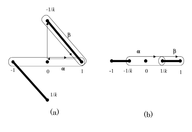
Figure 1. Geometry of Contours: $\alpha$ and $\beta$ are Homology basis of the elliptic curves.

Proof of Proposition 2.2: Let us consider the geometry of the integration. Fig.1 gives an illustration of our situations, where Fig.1 (a) corresponds to case I-1 and (b) does to case I-2.

1. The periodicity $(4\omega,2\omega^{\prime})$ of $\sqrt{(x-e_{a})}$ is given by

   $$\begin{split}\omega&=\int^{1}_{0}\frac{dw}{\sqrt{(1-w^{2})((\sqrt{e_{ba}}-\sqrt{e_{ca}})^{2}+4\sqrt{e_{ba}e_{ca}}w^{2})}},\\ \omega^{\prime}&=(\int^{0}_{1}+\int_{0}^{{\sqrt{-1}}/|k|})\frac{dw}{\sqrt{(1-w^{2})((\sqrt{e_{ba}}-\sqrt{e_{ca}})^{2}+4\sqrt{e_{ba}e_{ca}}w^{2})}}.\end{split}$$

   Thus $\omega_{2}=\omega_{1}/2+{\sqrt{-1}}L[k]$ for general $k$ with a certain function $L$. Hence $\tau=\omega^{\prime}/\omega\in(1/2+{\sqrt{-1}}{\mathbb{R}})$.

2. The periodicity $(4\omega,2\omega^{\prime})$ of $\sqrt{(x-e_{a})}$ is given by

   $$\begin{split}\omega&=2\int^{1/k}_{0}\frac{dw}{\sqrt{(1-w^{2})((\sqrt{e_{ba}}-\sqrt{e_{ca}})^{2}+4\sqrt{e_{ba}e_{ca}}w^{2})}},\\ \omega^{\prime}&=\int^{1}_{1/k}\frac{dw}{\sqrt{(1-w^{2})((\sqrt{e_{ba}}-\sqrt{e_{ca}})^{2}+4\sqrt{e_{ba}e_{ca}}w^{2})}}.\end{split}$$

   Hence $\tau=\omega^{\prime}/\omega\in{\sqrt{-1}}{\mathbb{R}}$.

   Since theory of the Jacobi elliptic functions gives the fact that $k^{\prime}:=\sqrt{1-k^{2}}$ gives the inversion of moduli $\tau\to-1/\tau$, the constraint $k>1$ is less important.

We note that the periodicity of $\sqrt{(x-e_{a})}$ differs from $\partial_{u}Z^{(a)}$ by twice but the difference is not so significant. Hence we have a complete proof of Proposition 2.2 based upon the theory of curve instead of geometry of Jacobain as a domain of theta function. ∎

Remark 2.2.

1. We list its spacial cases for $a=1$:

   1. $k=0$ in I-1: its shape is a circle and its related curve is $y^{2}=(x-e_{1})^{2}(x-e_{2})$

   2. $k=\infty$ in I-2: its shape is a loop soliton solution, and its related curve is $y^{2}=(x-e_{1})(x-e_{2})^{2}$

2. Since $\partial_{s}Z\equiv\mathrm{e}^{{\sqrt{-1}}\phi}$ can be regarded as a harmonic map: $\partial_{s}Z:S^{1}\to S^{1}$ with energy

   $$E=\oint ds|\partial_{s}\phi|^{2}.$$

3. Above Lemma 2.2, we argued the angle of $e_{ba}$’s. However the geometry of the integrals depends only $\sqrt{e_{ba}e_{ca}}$ and $\sqrt{e_{ba}}-\sqrt{e_{ca}}$ rather than $e_{ba}$’s themselves.

For the map $\partial_{u}Z:S^{1}\to S^{1}$, we can find index as a winding number as shown in Fig.2. We call it index($\partial_{u}Z$).

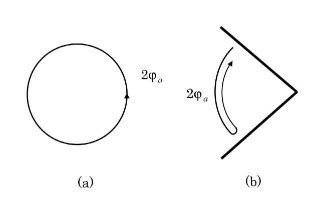
Figure 2. The behavior of $\varphi$

Corollary 2.1.

The $\mathrm{index}(\partial_{u}Z)$ is given as follows.

1. $\mathrm{index}(\partial_{u}Z)=1$.

2. $\mathrm{index}(\partial_{u}Z)=0$.

Proof.

In the case I-1, since the contours $w\equiv\sin\varphi_{a}$ is $[-1,1]$ which is identified with the range of sine function, $\varphi_{a}$ becomes a monotonic increasing function of $u$. In fact passing by $w=\pm 1$ changes the sign of $\sqrt{1-w^{2}}$ or $\cos\varphi_{a}$. On the other hand, in the case I-2, $\varphi$ does not wind around $S^{1}$ like Fig 2.(b). The branch point $(1/k,0)$ does not have an effect of the sign of $\sqrt{1-w^{2}}$. and thus it does not ∎

3. Genus Two

In this section, we will investigate the reality conditions of genus two. A hyperelliptic curve of genus two is expressed by

(3.1) $$\begin{split}y^{2}&=x^{5}+\lambda_{4}x^{4}+\lambda_{3}x^{3}+\lambda_{2}x^{2}+\lambda_{1}x+\lambda_{0}\\ &=(x-e_{1})(x-e_{2})(x-e_{3})(x-e_{4})(x-e_{5}),\end{split}$$

we have a coordinate of complex space $J^{\infty}_{2}:={\mathbb{C}}^{2}$;

(3.2) $$u_{1}=u_{1}^{(1)}+u_{1}^{(1)},\quad u_{2}=u_{2}^{(1)}+u_{2}^{(1)},$$

(3.3) $$u_{1}^{(i)}=\int^{(x^{(i)},y^{(i)})}_{\infty}\frac{dx}{2y},\quad u_{2}^{(i)}=\int^{(x^{(i)},y^{(i)})}_{\infty}\frac{xdx}{2y}.$$

The loop soliton solution of (3.1) is given by $\partial_{t_{1}}Z^{(a)}=(x^{(1)}-e_{a})(x^{(2)}-e_{a})$.

Lemma 3.1.

For different numbers $a$, $b$ and $c$ of $\{1,2,3\}$, let $\mathrm{e}^{2{\sqrt{-1}}\varphi_{a}^{(i)}}:=(x^{(i)}-e_{a})/c_{cba}$, $e_{ab}:=e_{a}-e_{b}$ and $c_{cba}:=\sqrt{e_{ba}e_{ca}}$. In general, the following relation holds:

$$du_{2}^{(i)}=\frac{{\sqrt{-1}}(c_{cba}\mathrm{e}^{{\sqrt{-1}}\varphi_{a}^{(i)}}+e_{a}\mathrm{e}^{-{\sqrt{-1}}\varphi_{a}^{(i)}})d\varphi_{a}^{(i)}}{\sqrt{((\sqrt{e_{ba}}-\sqrt{e_{ca}})^{2}+4\sqrt{e_{ba}e_{ca}}\sin^{2}\varphi_{a}^{(i)})c_{cba}e_{da}(\mathrm{e}^{-2{\sqrt{-1}}\varphi_{a}^{(i)}}-c_{cba}e_{da}^{-1})(\mathrm{e}^{2{\sqrt{-1}}\varphi_{a}^{(i)}}-c_{cba}^{-1}e_{ea})}}.$$

Proof.

Direct computations lead the formula. ∎

Lemma 3.2.

The reality condition of the loop soliton $Z^{(a)}$ satisfies if and only if $(x^{(1)},x^{(2)})\in\mathrm{Sym}^{2}(C_{2})$ and $\lambda$’s satisfy the following relations:

1. $|(x^{(i)}-e_{a})|=C_{a}$ of a real constant $C_{a}$, $(a=1,2)$,

2. $u_{2}^{(i)}\in{\mathbb{R}}$ for $i=1,2$.

Proof.

Since the satisfaction is trivial, we will consider the necessary condition. $(x^{(1)},x^{(2)})\in\mathrm{Sym}^{2}(C_{2})$ satisfying the reality conditions becomes

$$|x^{(2)}-e_{a}|=\frac{C}{|x^{(1)}-e_{a}|},$$

and

(3.4) $$\Im u_{2}^{(2)}(x^{(2)})=-\Im u_{2}^{(1)}(x^{(1)}).$$

Assume that $|x^{(1)}-e_{a}|$ or $\Im u_{2}^{(1)}(x^{(1)})$ is not a constant function of $x^{(1)}$. Then $x^{(2)}$ is a function of $x^{(1)}$. (Of course, there is no guarantee whether there exists such a function $x^{(2)}(x^{(1)})$ and even continuity.) On the other hand, the loop soliton $\partial_{t_{1}}Z^{(a)}$ is a function of the complex space $J^{\infty}_{2}$ in (3.2) and satisfies the MKdV equation (1.1) over there as mentioned in Proposition 1.1. However the assumption means that $u_{1}$ and $u_{2}$ are not independent, e.g., $u_{2}$ becomes a function of $u_{1}$. It implies that $\partial_{t_{1}}Z^{(a)}$ a function of a universal curve $C_{2}$ embedded in $J^{\infty}_{2}$ rather than $J^{\infty}_{2}$. ${\partial}/{\partial x^{(1)}}|_{x^{(2)}}$ nor ${\partial}/{\partial u_{1}}|_{u_{2}}$ do not behave well and should be replaced to covariant derivatives, e.g., ${\partial}/{\partial u_{1}}-A_{u_{1}}(u_{1})$, using an appropriate connection $A_{u_{1}}(u_{1})$. Hence in general the assumption requires that the angle part of $\partial_{t_{1}}Z^{(a)}$ does not satisfy the MKdV equation (1.1). It is a contradiction. ∎

Remark 3.1.

By letting the embedding $\iota:S^{1}\hookrightarrow C_{2}$, $\partial_{u_{2}}Z$ is a analytic map from $\mathrm{Sym}^{2}(\iota(S^{1}))$ to $S^{1}$.

Lemma 3.3.

For the situation of Lemma 3.1, the reality condition of the loop soliton $Z^{(a)}$ needs $e_{a}=-c_{cba}$ and $c_{eda}=c_{cba}$, and then we have

(3.5) $$du_{2}^{(i)}=\frac{2\sqrt{c_{cba}}\sin\varphi_{a}^{(i)}d\varphi_{a}^{(i)}}{\sqrt{((\sqrt{e_{ba}}-\sqrt{e_{ca}})^{2}+4\sqrt{e_{ba}e_{ca}}\sin^{2}\varphi_{a}^{(i)})((\sqrt{e_{da}}-\sqrt{e_{ea}})^{2}+4\sqrt{e_{da}e_{ea}}\sin^{2}\varphi_{a}^{(i)})}}.$$

Proof.

Due to the Lemma 3.2, $\varphi_{a}^{(i)}$ is real and each factor must be real. Hence the imaginary parts should be canceled locally. It means the conditions. ∎

Let us introduce a representation as an extension of the standard representation (2.4),

$$k_{1}:=\frac{2{\sqrt{-1}}\root 4 \of{e_{ba}e_{ca}}}{\sqrt{e_{ba}}-\sqrt{e_{ca}}},\quad k_{2}:=\frac{2{\sqrt{-1}}\root 4 \of{e_{da}e_{ea}}}{\sqrt{e_{da}}-\sqrt{e_{ea}}},$$

and then

(3.6) $$du_{2}^{(i)}=\frac{2\root 4 \of{e_{ba}e_{ca}}\sin\varphi_{a}^{(i)}d\varphi_{a}^{(i)}}{(\sqrt{e_{ba}}-\sqrt{e_{ca}})(\sqrt{e_{da}}-\sqrt{e_{ea}})\sqrt{1-k_{1}^{2}\sin^{2}\varphi_{a}^{(i)}}\sqrt{1-k_{2}^{2}\sin^{2}\varphi_{a}^{(i)}}}.$$

By letting $w:=\sin(\varphi_{a}^{(i)})$, we have

$$\begin{split}du_{2}^{(i)}&=\frac{\root 4 \of{e_{ba}e_{ca}}wdw}{\sqrt{(1-w^{2})((\sqrt{e_{ba}}-\sqrt{e_{ca}})^{2}+4\sqrt{e_{ba}e_{ca}}w^{2})((\sqrt{e_{da}}-\sqrt{e_{ea}})^{2}+4\sqrt{e_{da}e_{ea}}w^{2})}}\\ &=\frac{2\root 4 \of{e_{ba}e_{ca}}wdw}{(\sqrt{e_{ba}}-\sqrt{e_{ca}})(\sqrt{e_{da}}-\sqrt{e_{ea}})\sqrt{(1-w^{2})(1-k_{1}^{2}w^{2})(1-k_{2}^{2}w^{2})}}.\end{split}$$

Remark 3.2.

1. (3) is an elliptic integral by $u=w^{2}$ due to a speciality of genus two. It cannot be generalized to higher genus case.

2. Due to the remark 2.1, we should be regard that (3.6) gives the integral as a function $u_{2}^{(i)}$ of $\varphi_{a}^{(i)}$,

   $$u_{2}^{(i)}=\int^{\varphi_{a}^{(i)}}_{0}\frac{d\varphi_{a}^{(i)\prime}}{H_{a}^{[2]}(\varphi_{a}^{(i)\prime})}$$

   for an appropriate function $H_{2}^{[2]}$. Hence the inverse function $\varphi_{a}^{(i)}(u_{2}^{(i)})$ gives the relation,

   $$\exp({\sqrt{-1}}\varphi_{a}^{(i)}(u_{2}^{(i)}))=\sqrt{(x^{(i)}-e_{a})/c_{cba}}.$$

   Further $\varphi_{a}:=\varphi_{a}^{(1)}(u_{2}^{(1)})+\varphi_{a}^{(2)}(u_{2}^{(2)})$ gives the al-function of $u_{2}:=u_{2}^{(1)}+u_{2}^{(2)}$ [Ba, W],

   $$\exp({\sqrt{-1}}\varphi_{a}(u_{2}))=\mathrm{al}_{a}(u_{2}).$$

   Accordingly, we should regard this $\varphi_{a}$ as a hyperelliptic am-function of genus two.

3. Behind the hyperelliptic am-functions, there is also kinematic system with a hamitonian:

   $$E=\dot{w}^{2}+(1-w^{2})((\sqrt{e_{ba}}-\sqrt{e_{ca}})^{2}+4\sqrt{e_{ba}e_{ca}}w^{2})((\sqrt{e_{da}}-\sqrt{e_{ea}})^{2}+4\sqrt{e_{da}e_{ea}}w^{2}).$$

For any $\varphi_{a}^{(i)}$ in a region $[\varphi_{l},\varphi_{u}]$, the reality condition of the loop soliton $Z^{(a)}$ assumes that the denominator should be real and thus that $\sqrt{e_{ba}e_{ca}}$ and $\sqrt{e_{ba}}-\sqrt{e_{ca}}$ should be also real.

Theorem 3.1.

The reality condition of the loop soliton $Z^{(a)}$ is reduced to the conditions: $e_{a}=-c_{cba}$ and $c_{eda}=c_{cba}$ with three alternative cases:

1. $e_{ba}>0$, $e_{ca}>0$ $e_{ea}>0$, $e_{da}>0$, i.e., $k_{1},k_{2}\in{\sqrt{-1}}{\mathbb{R}}$ and $\sin\phi_{a}\in[-1,1]$.

2. $e_{ba}>0$, $e_{ca}>0$, $e_{ea}\leq 0$ and $e_{da}\leq 0$, i.e., $k_{1}\in{\sqrt{-1}}{\mathbb{R}}$ and $k_{2}\in{\mathbb{R}}$ $\sin\phi_{a}\in[1/k_{2},1]$ or $\sin\phi_{a}\in[-1,-1/k_{2}]$.

3. $e_{ba}\leq 0$, $e_{ca}\leq 0$ $e_{ea}\leq 0$, $e_{da}\leq 0$, i.e., $k_{1},k_{2}\in{\mathbb{R}}$, $(k_{1}<k_{2})$,

   1. if $k_{2}<1$, $\sin\phi_{a}\in[-1,1]$.

   2. if $k_{2}>1$, $\sin\phi_{a}\in[-1/k_{2},1/k_{2}]$.

   3. if $k_{1}>1$, $\sin\phi_{a}\in[1/k_{1},1]$ or $\sin\phi_{a}\in[-1,-1/k_{1}]$.

Proof.

As shown in case of the elliptic curves, we can find the results. ∎

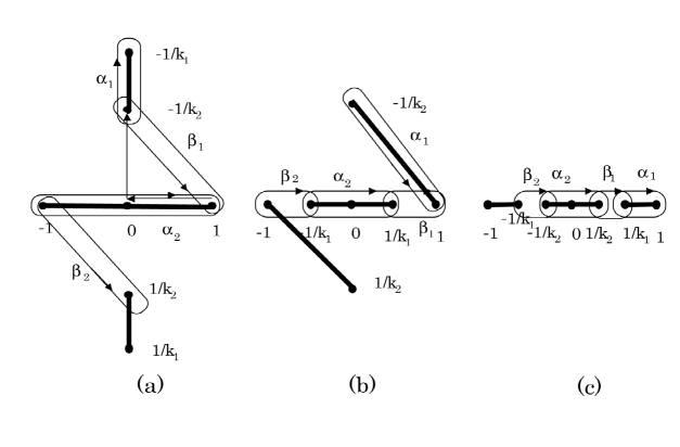
Figure 3. Geometry of Contours: $\alpha_{1}$, $\beta_{1}$, $\alpha_{2}$ and $\beta_{2}$ are Homology basis of the hyperelliptic curves.

Fig.3 gives an illustration of our situations, where Fig.3 (a) corresponds to II-1 and (b) does to II-2 and (c) to II-3.

In this case, we show the index($\partial_{t_{1}}Z$).

Corollary 3.1.

The $\mathrm{index}(\partial_{t_{1}}Z)$ as a winding number of the map $\iota(S^{1})$ to $S^{1}$ is

1. $\mathrm{index}(\partial_{t_{1}}Z)=2$,

2. $\mathrm{index}(\partial_{t_{1}}Z)=0$,

3. (a) $\mathrm{index}(\partial_{t_{1}}Z)=2$ and (b) (c) $\mathrm{index}(\partial_{t_{1}}Z)=0$.

Proof.

These indexes consist of those of each $2\varphi_{a}^{(i)}$. If the index of $2\varphi_{a}^{(i)}$ is one, that of $2\varphi_{a}$ is sum over $i=1,2$, $\varphi_{a}=\varphi_{a}^{(1)}+\varphi_{a}^{(2)}$. The computations of $\varphi_{a}$ are essentially the same as the genus one illustrated in Fig.2. ∎

4. Genus $g$

The computations of genus two are easily extended to higher genus loop solitons. Let ${\mathcal{A}}:=\{1,2,3,\cdots,2g+1\}$, ${\mathcal{A}}_{a}:={\mathcal{A}}-\{a\}$ for $a\in{\mathcal{A}}$, ${\mathcal{O}}_{g}:=\{1,3,5,\cdots,2g-1\}$. and a bijection $\sigma:\{1,2,\cdots,2g\}\to{\mathcal{A}}_{a}$ for $a\in{\mathcal{A}}$, which determines the order.

The direct computations give the following lemmas.

Lemma 4.1.

For $a\in{\mathcal{A}}$, let $\mathrm{e}^{2{\sqrt{-1}}\varphi_{a}^{(i)}}:=(x^{(i)}-e_{a})/c_{cba}$, $e_{ba}:=e_{\sigma(b)}-e_{a}$ and $c_{cba}:=\sqrt{e_{ba}e_{ca}}$,

(4.1) $$\begin{split}D^{(i)}_{a,\sigma}(\varphi_{a}):=&\Bigr{(}(\sqrt{e_{1a}}-\sqrt{e_{2a}})^{2}+4\sqrt{e_{1a}e_{2a}}\sin^{2}\varphi_{a}^{(i)})\\ &\prod_{d\in{\mathcal{O}}_{g},e=d+1}c_{12a}e_{da}(\mathrm{e}^{-2{\sqrt{-1}}\varphi_{a}^{(i)}}-c_{12a}e_{da}^{-1})(\mathrm{e}^{2{\sqrt{-1}}\varphi_{a}^{(i)}}-c_{12a}^{-1}e_{ea})\Bigr{)}^{1/2},\end{split}$$

$$N^{(i)}_{a,\sigma}(\varphi_{a}):=\left({\sqrt{-1}}(c_{12a}\mathrm{e}^{{\sqrt{-1}}\varphi_{a}^{(i)}}+e_{a}\mathrm{e}^{-{\sqrt{-1}}\varphi_{a}^{(i)}})\right)^{g-1}.$$

In general, (1.4) becomes

$$du_{g}^{(i)}=\frac{N^{(i)}_{a,\sigma}d\varphi_{a}}{D^{(i)}_{a,\sigma}}.$$

Lemma 4.2.

For the situation of Lemma 4.1, the reality condition of the loop soliton $Z^{(a)}$ needs $e_{a}=-c_{cba}$ for $c\in{\mathcal{A}}_{a}^{o}$, $b=c+1$ and then we have

(4.2) $$\begin{split}D^{(i)}_{a,\sigma}(\varphi_{a})&=\Bigr{(}((\sqrt{e_{1a}}-\sqrt{e_{2a}})^{2}+4\sqrt{e_{1a}e_{2a}}\sin^{2}\varphi_{a}^{(i)})\\ &\prod_{d\in{\mathcal{O}}_{g},e=d+1}((\sqrt{e_{da}}-\sqrt{e_{ea}})^{2}+4\sqrt{e_{da}e_{ea}}\sin^{2}\varphi_{a}^{(i)})\Bigr{)}^{1/2},\end{split}$$

$$N^{(i)}_{a,\sigma}(\varphi_{a})=\left(2\sqrt{c_{12a}}\sin\varphi_{a}^{(i)}\right)^{g-1}.$$

Let $\varphi_{a}:=\varphi_{a}^{(1)}+\varphi_{a}^{(2)}+\cdots+\varphi_{a}^{(g)}$ and then (1.5) is expressed by

$$\partial_{t_{1}}Z^{(a)}=\mathrm{e}^{2{\sqrt{-1}}\varphi_{a}},$$

as a function of $u_{g}:=u_{g}^{(1)}+u_{g}^{(2)}+\cdots+u_{g}^{(g)}$. The hyperelliptic al-function is written by

$$\mathrm{al}_{a}(u)=\mathrm{e}^{{\sqrt{-1}}\varphi_{a}(u)},$$

Hence $\varphi_{a}$ can be regarded as hyperelliptic am-function of genus $g$.

Theorem 4.1.

The reality condition of the loop soliton $Z^{(a)}$ in (1.5) is the conditions that there are $g$ pairs $(e_{b,a},e_{b+1,a})_{b\in{\mathcal{O}}_{g}}\in{\mathbb{R}}^{2}$ satisfying $-e_{a}=\sqrt{e_{b,a}e_{b+1,a}}\geq 0$, and the contour of integral of each $u^{(i)}_{g}$ of $i=1,\cdots,g$ should be chosen so that $u^{(i)}_{g}$ is real.

Shigeki Matsutani

e-mail:RXB01142nifty.com

8-21-1 Higashi-Linkan

Sagamihara 228-0811 Japan

References

[Ba]
H. F. Baker,
On the hyperelliptic sigma functions,
Amer. J. of Math.,
XX
(1898)
301-384.
[E] L. Euler,
Methodus inveniendi lineas curvas
maximi minimive proprietate gaudentes
1744,
Leonhardi Euleri Opera Omnia Ser. I Vol. 14
[Ma1]
S. Matstutani,
Hyperelliptic Loop Solitons with Genus :
Investigations of a Quantized Elastica,
J. Geom. Phys., 43 (2002) 146-162.
[Ma2]
by same author, On the Moduli of a Quantized Elastica in
and KdV Flows: Study of Hyperelliptic Curves as an
Extension of Euler’s Perspective of Elastica I,
Rev. Math. Phys., 15 559-628.
[Mu]
D. Mumford,
Elastica and Computer Vision, in
Algebraic Geometry and its Applications,
edited by C. Bajaj, Springer-Verlag, Berlin (1993)
507-518.
[P]
E. Previato,
Geometry of the Modified KdV Equation, in
Geometric and Quantum Aspects of Integrable System,
edited by G. F. Helminck, Springer-Verlag, Berlin (1993)
43-65.
[PS]
V. Prasolov and Y. Solovyev,
Elliptic Functions and Elliptic Integrals,
(1991) translated by D. Leites,
AMS, (1997) .
[W]
K. Weierstrass,
Zur Theorie der Abel’schen Functionen,
Aus dem Crelle’schen Journal,
47 (1854) .