On the Pauli operator for the Aharonov-Bohm effect with two solenoids

Abstract

We consider a spin-1/2 charged particle in the plane under the influence of two idealized Aharonov-Bohm fluxes. We show that the Pauli operator as a differential operator is defined by appropriate boundary conditions at the two vortices. Further we explicitly construct a basis in the deficiency subspaces of the symmetric operator obtained by restricting the domain to functions with supports separated from the vortices. This construction makes it possible to apply the Krein’s formula to the Pauli operator.

I Introduction

The goal of the present paper is to provide a more detailed analysis of the Pauli operator describing a spin-1/2 charged particle under the influence of two Aharonov-Bohm (AB) fluxes [1]. We consider the idealized setup when the magnetic fluxes are concentrated along two parallel lines so that the problem effectively reduces to a two-dimensional quantum system living in a perpendicular plane. In what follows we call the intersection points of the fluxes with the plane vortices.

To define the Pauli Hamiltonian with singular fluxes we use the Aharonov-Casher decomposition [2]. It makes it possible to introduce the two diagonal components of the Pauli operator corresponding to spin up and down as the unique selfadjoint operators associated to appropriate quadratic forms. Since the magnetic field vanishes outside of the vortices the two components of the Pauli Hamiltonian as well as the spinless AB Hamiltonian are selfadjoint extensions of the same symmetric operator. In the case of one AB flux all the selfadjoint extensions are known to be defined by appropriate boundary conditions at the vortex [3, 4]. Thus our first goal was to distinguish the boundary conditions defining the two components of the Pauli Hamiltonian.

The second goal was to construct a basis in the deficiency subspaces in the two-vortex case. In this case as well the two diagonal components of the Pauli Hamiltonian and the spinless Hamiltonian are selfadjoint extensions of a common symmetric operator. We show that the deficiency indices of this symmetric operator are $(4,4)$. The construction is based on the observation that the coefficients $\psi(x)$ standing at singular terms in the asymptotic expansion in the variable $x_{0}$ at a vortex of the Green function $\mathcal{G}_{z}(x,x_{0})$ belong to the deficiency subspace with spectral parameter $z$. Here we make use of the explicit knowledge of the spinless two-vortex Green function $\mathcal{G}_{z}(x,x_{0})$ [5].

The next and final goal which naturally follows is a construction of the two-vortex Green function for the Pauli Hamiltonian with the aid of the Krein’s formula. Even this problem is solved explicitly. Surprisingly many features can be again derived from the asymptotic analysis near a vortex.

The paper is organized as follows. In Section II we summarize some basic facts and formulae concerning the spinless AB Hamiltonian with one and two vortices. In Section III we introduce the Pauli operator with one and two AB fluxes and derive the boundary conditions at a vortex defining the spin up and down components of the Pauli Hamiltonian. In Section IV we provide a basic asymptotic analysis near a vortex of functions from the deficiency subspaces as well as that of the spinless Green function. In Section V we construct a basis in the deficiency subspaces. Section VI is devoted to the application of the Krein’s formula to our problem.

II Preliminaries. The AB Hamiltonian for a spinless particle

The AB Hamiltonian with one vortex and describing a spinless particle, $H_{0}$, was introduced in Ref. 1 and studied in a long series of papers by many authors. For example, one can consult Ref. 6 for some mathematical details. It acts in $L^{2}(\mathbb{R}^{2},\,\mathrm{d}^{2}x)$ and is nothing but the selfadjoint operator associated to the closure of the positive quadratic form

$$\int_{\mathbb{R}^{2}}\Bigg{(}\left|\left(\partial_{x_{1}}-\mathrm{i}\,\frac{\alpha\,x_{2}}{\left|x\right|^{2}}\right)\!\varphi\right|^{2}+\left|\left(\partial_{x_{2}}+\mathrm{i}\,\frac{\alpha\,x_{1}}{\left|x\right|^{2}}\right)\!\varphi\right|^{2}\Bigg{)}\,\mathrm{d}^{2}x\,,$$ (1)

defined on the space of test functions $\mathcal{D}(\mathbb{R}^{2}\setminus\{0\})$. In other words, $H_{0}$ is the Friedrichs extension of the corresponding symmetric operator with the domain $\mathcal{D}(\mathbb{R}^{2}\setminus\{0\})$. Owing to the gauge equivalence we can assume that $\alpha\in(0,1)$.

We shall use the polar coordinates $(r,\theta)$ with the angle $\theta\in(-\pi,\pi)$. This implies a cut along the negative $x_{1}$ half-axis. Sometimes it is convenient to apply the unitary operator

$$(U_{\alpha}\varphi)(r,\theta)=\mathrm{e}^{\mathrm{i}\,\alpha\,\theta}\varphi(r,\theta)$$

and work with the unitarily equivalent operator

$$H=U_{\alpha}H_{0}U_{\alpha}^{-1}.$$

In particular this unitary transformation is useful when constructing the Green function. This means that

$$\operatorname{Dom}(H)=U_{\alpha}(\operatorname{Dom}(H_{0}))\,.$$

Formally, as a differential operator,

$$H=-\Delta\,.$$

The domain of $H$ is determined by the boundary conditions at the cut, namely

$$\psi(r,\pi)=\mathrm{e}^{2\pi\,\mathrm{i}\,\alpha}\psi(r,-\pi),\textrm{ }\partial_{r}\psi(r,\pi)=\mathrm{e}^{2\pi\,\mathrm{i}\,\alpha}\partial_{r}\psi(r,-\pi)\,.$$ (2)

In addition, one should take care about boundary conditions at the vortex. As analyzed in Refs. 3, 4, the domain of $H_{0}$ is characterized by the boundary condition $\varphi(0)=0$. Since $\psi(r,\theta)=\exp(\mathrm{i}\alpha\theta)\varphi(r,\theta)$ the same is true for $\operatorname{Dom}(H)$, namely the boundary condition at the vortex reads $\psi(0)=0$.

The generalized eigenfunctions of $H$,

$$\left\{\frac{1}{\sqrt{2\pi}}\,J_{\left|n+\alpha\right|}(k\,r)\,\mathrm{e}^{\mathrm{i}(n+\alpha)\theta}\right\}_{k>0,\,n\in\mathbb{Z}},$$

form a complete normalized set,

$$\int_{0}^{\infty}J_{\nu}(k\,x)\,J_{\nu}(k\,y)\,k\,\mathrm{d}k=\frac{1}{x}\,\delta(x-y)\,.$$

This makes it possible to write down the Green function and the propagator as integrals,

$$\mathcal{G}_{z}(r,\theta;r_{0},\theta_{0})=\frac{1}{2\pi}\sum_{n\in\mathbb{Z}}\mathrm{e}^{\mathrm{i}(n+\alpha)(\theta-\theta_{0})}\int_{0}^{\infty}\frac{J_{\left|n+\alpha\right|}(k\,r)\,J_{\left|n+\alpha\right|}(k\,r_{0})}{k^{2}-z}\,k\,\mathrm{d}k$$ (3)

and

$$\mathcal{K}_{t}(r,\theta;r_{0},\theta_{0})=\frac{1}{2\pi}\sum_{n\in\mathbb{Z}}\mathrm{e}^{\mathrm{i}(n+\alpha)(\theta-\theta_{0})}\int_{0}^{\infty}\mathrm{e}^{-\mathrm{i}\,k^{2}t}J_{\left|n+\alpha\right|}(k\,r)\,J_{\left|n+\alpha\right|}(k\,r_{0})\,k\,\mathrm{d}k\,.$$ (4)

They are related by the Laplace transform,

$$\mathcal{G}_{z}(r,\theta;r_{0},\theta_{0})=\int_{0}^{\infty}\mathrm{e}^{z\,t}\,\mathcal{K}_{-\mathrm{i}\,t}(r,\theta;r_{0},\theta_{0})\,\mathrm{d}t\,.$$

Starting from (4) one can derive the following formula for the propagator[5],

$$\mathcal{K}_{t}(r,\theta;r_{0},\theta_{0}) = \left\{\begin{array}[]{c}1\\ \mathrm{e}^{2\pi\,\mathrm{i}\,\alpha}\\ \mathrm{e}^{-2\pi\,\mathrm{i}\,\alpha}\end{array}\right\}\frac{1}{4\pi\,\mathrm{i}\,t}\exp\!\Big{(}-\frac{1}{4\mathrm{i}\,t}\left|x-x_{0}\right|^{2}\Big{)}$$

$$-\frac{\sin(\pi\,\alpha)}{\pi}\int_{-\infty}^{\infty}\frac{1}{4\pi\,\mathrm{i}\,t}\exp\!\Big{(}-\frac{1}{4\mathrm{i}\,t}\,R(s)^{2}\Big{)}\frac{\mathrm{e}^{-\alpha\,s+\mathrm{i}\,\alpha\,(\theta-\theta_{0})}}{1+\mathrm{e}^{-s+\mathrm{i}\,(\theta-\theta_{0})}}\,\,\mathrm{d}s\,,$$

where

$$\left|x-x_{0}\right|^{2}=r^{2}+r_{0}^{2}-2r\,r_{0}\cos(\theta-\theta_{0}),\textrm{ }R(s)^{2}=r^{2}+r_{0}^{2}+2r\,r_{0}\cosh(s),$$

and the phase factor in front of the first term depends on whether

$$\theta-\theta_{0}\in(-\pi,\pi),\textrm{ }(\pi,2\pi)\textrm{ or }(-2\pi,-\pi).$$

The Laplace transformation results in a formula for the Green function,

$$\mathcal{G}_{z}(r,\theta;r_{0},\theta_{0}) = \left\{\begin{array}[]{c}1\\ \mathrm{e}^{2\pi\,\mathrm{i}\,\alpha}\\ \mathrm{e}^{-2\pi\,\mathrm{i}\,\alpha}\end{array}\right\}\frac{1}{2\pi}\,K_{0}\!\left(\sqrt{-z}\left|x-x_{0}\right|\right)$$

$$-\frac{\sin(\pi\,\alpha)}{\pi}\int_{-\infty}^{\infty}\frac{1}{2\pi}\,K_{0}\Big{(}\sqrt{-z}\,R(s)\Big{)}\frac{\mathrm{e}^{-\alpha\,s+\mathrm{i}\,\alpha\,(\theta-\theta_{0})}}{1+\mathrm{e}^{-s+\mathrm{i}\,(\theta-\theta_{0})}}\,\,\mathrm{d}s\,.$$

The second term on the RHS of (II) can be given still another form with the aid of the identity

$$\int_{-\infty}^{\infty}K_{\mathrm{i}\tau}(a)\,K_{-\mathrm{i}\tau}(b)\,\frac{\mathrm{e}^{\phi\,\tau}}{\sin(\pi(\alpha+\mathrm{i}\tau))}\,\mathrm{d}\tau$$

$$\qquad\quad=\,\int_{-\infty}^{\infty}K_{0}\!\left(\sqrt{a^{2}+b^{2}+2\,a\,b\,\cosh(u)}\,\right)\frac{\mathrm{e}^{-\alpha(u-\mathrm{i}\,\phi)}}{1+\mathrm{e}^{-u+\mathrm{i}\,\phi}}\,\,\mathrm{d}u$$

for $a>0$, $b>0$, $0<\alpha<1$ and $\left|\phi\right|<\pi$. This way we get

$$\mathcal{G}_{z}(r,\theta;r_{0},\theta_{0}) = \frac{1}{2\pi}K_{0}\!\left(\sqrt{-z}\left|x-x_{0}\right|\right)$$

$$-\frac{\sin(\pi\,\alpha)}{2\pi^{2}}\int_{-\infty}^{\infty}K_{\mathrm{i}\tau}\!\left(\sqrt{-z}\,r\right)\,K_{-\mathrm{i}\tau}\!\left(\sqrt{-z}\,r_{0}\right)\,\frac{\mathrm{e}^{(\theta-\theta_{0})\,\tau}}{\sin(\pi(\alpha+\mathrm{i}\,\tau))}\,\,\mathrm{d}\tau\,$$

for $$\theta-\theta_{0}\in(-\pi,\pi)$$,

$$\mathcal{G}_{z}(r,\theta;r_{0},\theta_{0}) = \mathrm{e}^{2\pi\,\mathrm{i}\,\alpha}\Bigg{(}\frac{1}{2\pi}K_{0}\left(\sqrt{-z}\left|x-x_{0}\right|\right)$$

$$-\frac{\sin(\pi\,\alpha)}{2\pi^{2}}\int_{-\infty}^{\infty}K_{\mathrm{i}\tau}\!\left(\sqrt{-z}\,r\right)\,K_{-\mathrm{i}\tau}\!\left(\sqrt{-z}\,r_{0}\right)\,\frac{\mathrm{e}^{(\theta-\theta_{0}-2\pi)\,\tau}}{\sin(\pi(\alpha+\mathrm{i}\,\tau))}\,\,\mathrm{d}\tau\Bigg{)}$$

for $$\theta-\theta_{0}\in(\pi,2\pi)$$, and

$$\mathcal{G}_{z}(r,\theta;r_{0},\theta_{0}) = \mathrm{e}^{-2\pi\,\mathrm{i}\,\alpha}\Bigg{(}\frac{1}{2\pi}K_{0}\!\left(\sqrt{-z}\left|x-x_{0}\right|\right)$$

$$-\frac{\sin(\pi\,\alpha)}{2\pi^{2}}\int_{-\infty}^{\infty}K_{\mathrm{i}\tau}\!\left(\sqrt{-z}\,r\right)\,K_{-\mathrm{i}\tau}\!\left(\sqrt{-z}\,r_{0}\right)\,\frac{\mathrm{e}^{(\theta-\theta_{0}+2\pi)\,\tau}}{\sin(\pi(\alpha+\mathrm{i}\,\tau))}\,\,\mathrm{d}\tau\Bigg{)}$$

for $$\theta-\theta_{0}\in(-2\pi,-\pi)$$.

Despite of this threefold description depending on the value of $\theta-\theta_{0}$ the Green function should be continuous, even real analytic, in its domain of definition if $x\neq x_{0}$. Checking the limits from the right and left for $\theta-\theta_{0}=\pm\pi$ one finds that the continuity is guaranteed by the identity

$$\int_{-\infty}^{\infty}K_{\mathrm{i}\,\tau}(a)\,K_{-\mathrm{i}\,\tau}(b)\,\mathrm{d}\tau=\pi\,K_{0}(a+b)\quad\textrm{for }\,a>0,\,b>0.$$

Let us add a remark on deficiency subspaces. First we recall a general and easy to verify fact. Let $A$ be a selfadjoint extension of a symmetric operator $X$. Denote by $\mathcal{N}(z)=\operatorname{Ker}(X^{*}-z)$ the deficiency subspaces, $\operatorname{Im}\,z\neq 0$. Then it holds

$$f\in\mathcal{N}(w)\,\Longrightarrow\,f+(z-w)(A-z)^{-1}f\in\mathcal{N}(z)\,.$$

This can be illustrated on our problem. We choose $H$ (the one-vortex AB Hamiltonian defined by the boundary conditions (2)) for $A$, and $X$ is a restriction of $H$ obtained by requiring the supports of functions from the domain of $X$ to be separated from the singular point (the origin). The deficiency indices are known to be $(2,2)$. For a basis in $\mathcal{N}(z)$ we can choose the vectors

$$\psi_{-1,z}(r,\theta)=K_{1-\alpha}\!\left(\sqrt{-z}\,r\right)\mathrm{e}^{\mathrm{i}(\alpha-1)\theta},\textrm{ }\psi_{0,z}(r,\theta)=K_{\alpha}\!\left(\sqrt{-z}\,r\right)\mathrm{e}^{\mathrm{i}\,\alpha\,\theta}\,.$$ (14)

Here $z\in\mathbb{C}\setminus\mathbb{R}_{+}$, $\operatorname{Re}\,\sqrt{-z}>0$. As shown in Ref. 3 it holds true that

$$\int_{0}^{\infty}\left(\int_{-\pi}^{\pi}\mathcal{G}_{z}(r,\theta;r_{0},\theta_{0})\,\psi_{0,w}(r_{0},\theta_{0})\,\mathrm{d}\theta_{0}\right)r_{0}\,\mathrm{d}r_{0}$$

$$\qquad\quad=\,\frac{1}{z-w}\,\mathrm{e}^{\mathrm{i}\,\alpha\,\theta}\left(\left(\frac{\sqrt{-z}}{\sqrt{-w}}\right)^{\!\alpha}K_{\alpha}\!\left(\sqrt{-z}\,r\right)-K_{\alpha}\!\left(\sqrt{-w}\,r\right)\right),$$

hence

$$\psi_{0,w}+(z-w)(H-z)^{-1}\psi_{0,w}=\left(\frac{\sqrt{-z}}{\sqrt{-w}}\right)^{\!\alpha}\psi_{0,z}\,.$$ (15)

Similarly,

$$\psi_{-1,w}+(z-w)(H-z)^{-1}\psi_{-1,w}=\left(\frac{\sqrt{-z}}{\sqrt{-w}}\right)^{\!1-\alpha}\psi_{-1,z}\,.$$ (16)

Let us now focus on the case of two vortices but still considering a spineless particle. The vortices are supposed to be located in the points $a=(0,0)$ and $b=(\rho,0)$, $\rho>0$. Let $(r_{a},\theta_{a})$ be the polar coordinates centered at the point $a$ and $(r_{b},\theta_{b})$ be the polar coordinates centered at the point $b$. The two-vortex AB Hamiltonian $H_{0}$ is the unique self-adjoint operator associated to the quadratic form

$$\int_{\mathbb{R}^{2}}\left(\left|\left(-\mathrm{i}\,\partial_{x_{1}}-A_{1}\right)\!\varphi\right|^{2}+\left|\left(-\mathrm{i}\,\partial_{x_{2}}-A_{2}\right)\!\varphi\right|\right)^{2}\,\mathrm{d}^{2}x\,,$$ (17a)

where

$$A=-\alpha\,\mathrm{d}\theta_{a}-\beta\,\mathrm{d}\theta_{b}.$$ (17b)

Again, owing to the gauge equivalence, we can assume that $\alpha,\beta\in(0,1)$.

Also in this case one can pass to a unitarily equivalent formulation. The plane is cut along two half-lines,

$$L_{a}=(-\infty,0)\times\{0\}\textrm{ and }L_{b}=(\rho,+\infty)\times\{0\}.$$

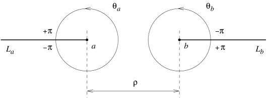
Figure 1: Geometrical arrangement. Choice of the cuts $L_{a}$, $L_{b}$ and choice of the angle variables $\theta_{a}$, $\theta_{b}$.

The values $\theta_{a}=\pm\pi$ correspond to the two sides of the cut $L_{a}$ and similarly for $\theta_{b}$ and $L_{b}$. The geometrical arrangement is sketched in Fig. 1. The unitarily equivalent Hamiltonian $H$ is formally equal to $-\Delta$ and is determined by the boundary conditions along the cut,

$$\psi(r_{a},\theta_{a}=\pi)=\mathrm{e}^{2\pi\,\mathrm{i}\,\alpha}\psi(r_{a},\theta_{a}=-\pi),\textrm{ }\partial_{r_{a}}\psi(r_{a},\theta_{a}=\pi)=\mathrm{e}^{2\pi\,\mathrm{i}\,\alpha}\partial_{r_{a}}\psi(r,\theta_{a}=-\pi)\,,$$

$$\psi(r_{b},\theta_{b}=\pi)=\mathrm{e}^{2\pi\,\mathrm{i}\,\beta}\psi(r_{b},\theta_{b}=-\pi),\textrm{ }\partial_{r_{b}}\psi(r_{b},\theta_{b}=\pi)=\mathrm{e}^{2\pi\,\mathrm{i}\,\beta}\partial_{r_{b}}\psi(r,\theta_{b}=-\pi)\,.$$ (18)

In addition, one should impose a boundary condition at the vortex, namely $\psi(a)=\psi(b)=0$.

A formula for the Green function of the Hamiltonian $H$ is known also in the case of two vortices [5]. For a couple of points $x,x_{0}\in\mathbb{R}^{2}\setminus(L_{a}\cup L_{b})$ we set

$$\zeta_{a}=1\textrm{ or }\zeta_{a}=\mathrm{e}^{2\,\pi\,\mathrm{i}\,\alpha}\textrm{ or }\zeta_{a}=\mathrm{e}^{-2\,\pi\,\mathrm{i}\,\alpha}$$

depending on whether the segment $\overline{x_{0}x}$ does not intersect $L_{a}$, or $\overline{x_{0}x}$ intersects $L_{a}$ and $x_{0}$ lies in the lower half-plane, or $\overline{x_{0}x}$ intersects $L_{a}$ and $x_{0}$ lies in the upper half-plane. Analogously,

$$\zeta_{b}=1\textrm{ or }\zeta_{b}=\mathrm{e}^{2\,\pi\,\mathrm{i}\,\beta}\textrm{ or }\zeta_{b}=\mathrm{e}^{-2\,\pi\,\mathrm{i}\,\beta}$$

depending on whether the segment $\overline{x_{0}x}$ does not intersect $L_{b}$, or $\overline{x_{0}x}$ intersects $L_{b}$ and $x_{0}$ lies in the upper half-plane, or $\overline{x_{0}x}$ intersects $L_{b}$ and $x_{0}$ lies in the lower half-plane. Furthermore, let us set

$$\zeta_{a}=\mathrm{e}^{\mathrm{i}\,\alpha\,\eta_{a}},\,\,\zeta_{b}=\mathrm{e}^{\mathrm{i}\,\beta\,\eta_{b}}\quad\textrm{where }\eta_{a},\eta_{b}\in\{0,2\,\pi,-2\,\pi\}.$$

Remark.

Notice that if $\zeta_{a}\neq 1$ then necessarily $\zeta_{b}=1$ and vice versa.

The formula for the Green function reads

$$\mathcal{G}_{z}(x,x_{0})=\zeta_{a}\zeta_{b}\frac{1}{2\,\pi}\,K_{0}\!\left(\sqrt{-z}\left|x-x_{0}\right|\right)$$

$$-\,\zeta_{a}\frac{\sin(\pi\,\alpha)}{2\pi^{2}}\int_{-\infty}^{\infty}K_{\mathrm{i}\tau}\!\left(\sqrt{-z}\,r_{a}\right)\,K_{-\mathrm{i}\tau}\!\left(\sqrt{-z}\,r_{0a}\right)\,\frac{\mathrm{e}^{(\theta_{a}-\theta_{0a}-\eta_{a})\tau}}{\sin(\pi(\alpha+\mathrm{i}\tau))}\,\mathrm{d}\tau$$

$$-\,\zeta_{b}\frac{\sin(\pi\,\beta)}{2\pi^{2}}\int_{-\infty}^{\infty}K_{\mathrm{i}\tau}\!\left(\sqrt{-z}\,r_{b}\right)\,K_{-\mathrm{i}\tau}\!\left(\sqrt{-z}\,r_{0b}\right)\,\frac{\mathrm{e}^{(\theta_{b}-\theta_{0b}-\eta_{b})\tau}}{\sin(\pi(\beta+\mathrm{i}\tau))}\,\mathrm{d}\tau$$

$$+\,\frac{1}{2\pi}\sum_{\gamma,\,n\geq 2}(-1)^{n}\int_{\mathbb{R}^{n}}K_{\mathrm{i}\tau_{n}}\!\left(\sqrt{-z}\,r\right)K_{\mathrm{i}(\tau_{n-1}-\tau_{n})}\!\left(\sqrt{-z}\,\rho\right)$$ (19)

$$\quad\times\ldots\times K_{\mathrm{i}(\tau_{1}-\tau_{2})}\!\left(\sqrt{-z}\,\rho\right)K_{-\mathrm{i}\tau_{1}}\!\left(\sqrt{-z\,}r_{0}\right)\,\frac{\sin(\pi\,\sigma_{n})\,\exp(\theta\,\tau_{n})}{\pi\,\sin(\pi(\sigma_{n}+\mathrm{i}\tau_{n}))}$$

$$\quad\times\,\frac{\sin(\pi\,\sigma_{n-1})}{\pi\sin(\pi(\sigma_{n-1}+\mathrm{i}\tau_{n-1}))}\times\ldots\times\frac{\sin(\pi\,\sigma_{2})}{\pi\sin(\pi(\sigma_{2}+\mathrm{i}\tau_{2}))}\,\frac{\sin(\pi\,\sigma_{1})\,\exp(-\theta_{0}\tau_{1})}{\pi\sin(\pi(\sigma_{1}+\mathrm{i}\tau_{1}))}\,\,\mathrm{d}^{n}\tau\,.$$

Here the sum $\sum_{\gamma,\,n\geq 2}$ runs over all finite alternating sequences of length at least two, $\gamma=(c_{n},c_{n-1},\ldots,c_{1})$, such that for all $j$, $c_{j}\in\{a,b\}$ and $c_{j}\neq c_{j+1}$, and $\sigma_{j}=\alpha$ (resp. $\beta$) depending on whether $c_{j}=a$ (resp. $b$). In addition, $(r,\theta)$ are the polar coordinates of the point $x$ with respect to the center $c_{n}$, $(r_{0},\theta_{0})$ are the polar coordinates of the point $x_{0}$ with respect to the center $c_{1}$(the dependence on $\gamma$ is not indicated explicitly).

III The Pauli Hamiltonian with AB fluxes

According to the Aharonov-Casher ansatz [2] the two diagonal components of the Pauli Hamiltonian with the third component of spin equal to $\pm 1/2$ can be factorized,

$$H^{\pm}=(p-A)^{2}\mp B=P_{\pm}^{*}P_{\pm}\,,$$

where

$$P_{\pm}=(p_{1}-A_{1})\pm\mathrm{i}\,(p_{2}-A_{2}).$$

Using the complex coordinate $z=x_{1}+\mathrm{i}\,x_{2}$ one can rewrite the Pauli Hamiltonian as follows:

$$H^{+} = 4(-\mathrm{i}\,\partial_{z}-A_{z})(-\mathrm{i}\,\partial_{\overline{z}}-A_{\overline{z}}),$$

$$H^{-} = 4(-\mathrm{i}\,\partial_{\overline{z}}-A_{\overline{z}})(-\mathrm{i}\,\partial_{z}-A_{z}).$$

We start our discussion from considering the situation with one vortex. Then

$$A=\frac{\alpha}{r^{2}}(x_{2}\,\,\mathrm{d}x_{1}-x_{1}\,\mathrm{d}x_{2})=-\alpha\,\,\mathrm{d}\theta=\frac{\mathrm{i}\,\alpha}{2}\,\mathrm{e}^{-2\mathrm{i}\,\theta}\,\mathrm{d}\mathrm{e}^{2\mathrm{i}\,\theta}=\frac{\mathrm{i}\,\alpha}{2}\frac{\overline{z}}{z}\,\mathrm{d}\frac{z}{\overline{z}}=\frac{\mathrm{i}\,\alpha}{2}\Big{(}\frac{\,\mathrm{d}z}{z}-\frac{\,\mathrm{d}\overline{z}}{\overline{z}}\Big{)}.$$

Hence

$$A_{z}=\frac{\mathrm{i}\,\alpha}{2z},\textrm{ }A_{\overline{z}}=-\frac{\mathrm{i}\,\alpha}{2\overline{z}},$$

and we can write

$$H^{+}=-4\Big{(}\,\partial_{z}+\frac{\alpha}{2z}\Big{)}\Big{(}\,\partial_{\overline{z}}-\frac{\alpha}{2\overline{z}}\Big{)},\textrm{ }H^{-}=-4\Big{(}\,\partial_{\overline{z}}-\frac{\alpha}{2\overline{z}}\Big{)}\Big{(}\,\partial_{z}+\frac{\alpha}{2z}\Big{)}.$$

In fact, these are formal expressions. More precisely, the operators are defined as the unique selfadjoint operators associated respectively to the positive quadratic forms

$$\mathfrak{q}_{+}(\varphi)=4\int_{\mathbb{R}^{2}}\left|\Big{(}\partial_{\overline{z}}-\frac{\alpha}{2\overline{z}}\Big{)}\varphi\right|^{2}\,\mathrm{d}^{2}x\,,\textrm{ }\mathfrak{q}_{-}(\varphi)=4\int_{\mathbb{R}^{2}}\left|\Big{(}\partial_{z}+\frac{\alpha}{2z}\Big{)}\varphi\right|^{2}\,\mathrm{d}^{2}x\,,$$ (20)

with their natural maximal domains of definition.

Since the magnetic field vanishes on $\mathbb{R}^{2}\setminus\{0\}$ the operators $H^{\pm}$ coincide with the spinless AB Hamiltonian $H_{0}$ on the domain $\mathcal{D}(\mathbb{R}^{2}\setminus\{0\})$ ($\mathcal{D}$ is the space of test functions). This means that all three operators $H^{+}$, $H^{-}$ and $H_{0}$ are selfadjoint extensions of the same symmetric operator $\widetilde{X}$. From Refs. 3 and 4 it is known that all selfadjoint extensions can be described by appropriate boundary conditions at the origin. The method used to derive the boundary conditions was inspired by the description of point interactions in the plane given in Ref. 7. Let us also note that analogous boundary conditions have been derived in Ref. 8 for the model with additional homogeneous magnetic field while the case of Dirac-Weyl operator is discussed in Ref. 9.

To describe the boundary conditions one introduces four functionals,

$$\Phi_{1}^{-1}(\varphi) = \lim_{r\downarrow 0}\,r^{1-\alpha}\frac{1}{2\pi}\int_{0}^{2\pi}\varphi(r,\theta)\,\mathrm{e}^{\mathrm{i}\,\theta}\,\mathrm{d}\theta,$$

$$\Phi_{2}^{-1}(\varphi) = \lim_{r\downarrow 0}\,r^{-1+\alpha}\left(\frac{1}{2\pi}\int_{0}^{2\pi}\varphi(r,\theta)\,\mathrm{e}^{\mathrm{i}\,\theta}\,\mathrm{d}\theta-r^{-1+\alpha}\Phi_{1}^{-1}(\varphi)\right),$$

$$\Phi_{1}^{0}(\varphi) = \lim_{r\downarrow 0}\,r^{\alpha}\frac{1}{2\pi}\int_{0}^{2\pi}\varphi(r,\theta)\,\mathrm{d}\theta,$$

$$\Phi_{2}^{0}(\varphi) = \lim_{r\downarrow 0}\,r^{-\alpha}\left(\frac{1}{2\pi}\int_{0}^{2\pi}\varphi(r,\theta)\,\mathrm{d}\theta-r^{-\alpha}\Phi_{1}^{0}(\varphi)\right).$$

Each boundary condition is determined by a couple of matrices $A_{1},A_{2}\in\operatorname{Mat}(2,\mathbb{C})$ fulfilling (the symbol $(A_{1},A_{2})$ designates a $2\times 4$ matrix)

$$\operatorname{rank}\,(A_{1},A_{2})=2,\textrm{ }A_{1}D^{-1}A_{2}^{*}=A_{2}D^{-1}A_{1}^{*}$$

where

$$D=\begin{pmatrix}1-\alpha&0\\ 0&\alpha\end{pmatrix}.$$

The boundary condition takes the form

$$A_{1}\begin{pmatrix}\Phi_{1}^{-1}(\varphi)\\ \Phi_{1}^{0}(\varphi)\end{pmatrix}+A_{2}\begin{pmatrix}\Phi_{2}^{-1}(\varphi)\\ \Phi_{2}^{0}(\varphi)\end{pmatrix}=\begin{pmatrix}0\\ 0\end{pmatrix}.$$

Two couples of matrices, $\{A_{1},A_{2}\}$ and $\{A^{\prime}_{1},A^{\prime}_{2}\}$, determine the same boundary condition if and only if there exists a regular matrix $G\in\operatorname{GL}(2,\mathbb{C})$ such that $(A^{\prime}_{1},A^{\prime}_{2})=G(A_{1},A_{2})$.

For example, the domain of the spinless AB Hamiltonian $H_{0}$ is determined by the boundary conditions at the vortex $\Phi_{1}^{-1}(\varphi)=\Phi_{1}^{0}(\varphi)=0$ and so by the couple of matrices

$$A_{1}=\begin{pmatrix}1&0\\ 0&1\end{pmatrix},\textrm{ }A_{2}=\begin{pmatrix}0&0\\ 0&0\end{pmatrix}.$$

We wish to derive the boundary conditions for the Hamiltonians $H^{+}$ and $H^{-}$. According to the well-known construction, the operator $A$ associated to a semi-bounded quadratic form $\mathfrak{q}$ is determined by the condition

$$\forall f\in\operatorname{Dom}(A)\subset\operatorname{Dom}(\mathfrak{q}),\,\forall\varphi\in\operatorname{Dom}(\mathfrak{q}),\textrm{ }\langle\varphi,Af\rangle=\mathfrak{q}(\varphi,f)\,.$$

This is to say that $f\in\operatorname{Dom}(\mathfrak{q})$ belongs to $\operatorname{Dom}(A)$ if and only if there exists $g\in\mathcal{H}$ such that the equality $\langle\varphi,g\rangle=\mathfrak{q}(\varphi,f)$ holds true for all $\varphi\in\operatorname{Dom}(\mathfrak{q})$. In that case $g$ is unique and $Af=g$. We are going to apply this prescription to the quadratic forms (20). This amounts to integration by parts.

More precisely, the Green formula implies that

$$\int_{\mathbb{R}^{2}}(\partial_{z}f)g\,\mathrm{d}^{2}x=-\int_{\mathbb{R}^{2}}f(\partial_{z}g)\,\mathrm{d}^{2}x-\lim_{a\downarrow 0}\,\frac{a}{2}\int_{0}^{2\pi}(f\,g)(a\,\cos(\theta),a\,\sin(\theta))\,\mathrm{e}^{-\mathrm{i}\,\theta}\,\mathrm{d}\theta\,.$$

Thus one finds that $f\in\operatorname{Dom}(\widetilde{X}^{*})$ belongs to $\operatorname{Dom}(H^{+})$ if and only if for all $\varphi\in\operatorname{Dom}(\mathfrak{q}_{+})$,

$$\lim_{a\downarrow 0}\,a\int_{0}^{2\pi}\Big{(}\overline{\varphi}\,\Big{(}\,\partial_{\overline{z}}-\frac{\alpha}{2\overline{z}}\Big{)}f\Big{)}(a\,\cos(\theta),a\,\sin(\theta))\,{{\mathrm{e}}^{-\mathrm{i}\,\theta}}\,\mathrm{d}\theta\,=0,$$

or, when expressing $(z,\overline{z})$ in the polar coordinates,

$$\lim_{a\downarrow 0}\,\int_{0}^{2\pi}\big{(}\overline{\varphi}\,(\,r\,\partial_{r}+\mathrm{i}\,\partial_{\theta}-\alpha)f\big{)}(a\cos(\theta),a\sin(\theta))\,\mathrm{d}\theta\,=0.$$

Any $f\in\operatorname{Dom}(\widetilde{X}^{*})$ asymptotically behaves like

$$f=\left(\Phi_{1}^{-1}(f)\,r^{-1+\alpha}+\Phi_{2}^{-1}(f)\,r^{1-\alpha}\right)\mathrm{e}^{-\mathrm{i}\,\theta}+\left(\Phi_{1}^{0}(f)\,r^{-\alpha}+\Phi_{2}^{0}(f)\,r^{\alpha}\right)+\textrm{ regular part}.$$

Hence

$$(r\,\partial_{r}+\mathrm{i}\,\partial_{\theta}-\alpha)f\sim 2(1-\alpha)\Phi_{2}^{-1}(f)\,r^{1-\alpha}\mathrm{e}^{-\mathrm{i}\,\theta}-2\alpha\,\Phi_{1}^{0}(f)\,r^{-\alpha}+\ldots\,.$$

Notice that

$$(r\,\partial_{r}+\mathrm{i}\,\partial_{\theta}-\alpha)r^{-1+\alpha}\mathrm{e}^{-\mathrm{i}\,\theta}=(r\,\partial_{r}+\mathrm{i}\,\partial_{\theta}-\alpha)r^{\alpha}=0$$

and so any function of the form $r^{-1+\alpha}\eta(r)\mathrm{e}^{-\mathrm{i}\,\theta}$ or $r^{\alpha}\eta(r)$, with $\eta\in{}C^{\infty}(\mathbb{R}_{+})$, $\eta(r)\equiv 1$ in a neighborhood of 0 and $\eta(r)\equiv 0$ in a neighborhood of $+\infty$, belongs to $\operatorname{Dom}(\mathfrak{q}_{+})$. Therefore a sufficient and necessary condition for $f$ to belong to $\operatorname{Dom}(H^{+})$ is

$$\Phi_{2}^{-1}(f)\,=\Phi_{1}^{0}(f)=0.$$ (21)

The corresponding couple of matrices can be chosen as

$$A_{1}=\begin{pmatrix}0&1\\ 0&0\end{pmatrix},\textrm{ }A_{2}=\begin{pmatrix}0&0\\ 1&0\end{pmatrix}$$

The other component of the Pauli Hamiltonian, $H^{-}$, can be treated similarly. One finds that $f\in\operatorname{Dom}(\widetilde{X}^{*})$ belongs to $\operatorname{Dom}(H^{-})$ if and only if for all $\varphi\in\operatorname{Dom}(\mathfrak{q}_{-})$,

$$\lim_{a\downarrow 0}\,\int_{0}^{2\pi}\big{(}\overline{\varphi}\,(r\,\partial_{r}-\mathrm{i}\,\partial_{\theta}+\alpha)f\big{)}(a\cos(\theta),a\sin(\theta))\,\mathrm{d}\theta=0$$

which turns out to be equivalent to

$$\Phi_{1}^{-1}(f)=\Phi_{2}^{0}(f)=0.$$ (22)

The corresponding couple of matrices can be chosen as

$$A_{1}=\begin{pmatrix}1&0\\ 0&0\end{pmatrix},\textrm{ }A_{2}=\begin{pmatrix}0&0\\ 0&1\end{pmatrix}.$$

The generalization to the case of several vortices is quite straightforward. One simply imposes the above derived boundary conditions at each vortex. Let us consider the case of two vortices. For the sake of simplicity we assume that the vortices are $a=(0,0)$ and $b=(1,0)$. The Pauli Hamiltonian formally reads

$$H^{+} = -4\left(\partial_{z}+\frac{1}{2}\Big{(}\frac{\alpha}{z}+\frac{\beta}{z-1}\Big{)}\right)\left(\partial_{\overline{z}}-\frac{1}{2}\Big{(}\frac{\alpha}{\overline{z}}+\frac{\beta}{\overline{z}-1}\Big{)}\right),$$

$$H^{-} = -4\left(\partial_{\overline{z}}-\frac{1}{2}\Big{(}\frac{\alpha}{\overline{z}}+\frac{\beta}{\overline{z}-1}\Big{)}\right)\left(\partial_{z}+\frac{1}{2}\Big{(}\frac{\alpha}{z}+\frac{\beta}{z-1}\Big{)}\right).$$

We still assume that $0<\alpha,\beta<1$ (in virtue of the gauge equivalence).

The Pauli Hamiltonian with two vortices is known to have zero modes [10]. They can be computed with the aid of the Aharonov-Casher ansatz since it effectively enables to reduce the second order differential equation to a first order one. Explicit solutions are even known in some essentially more complicated situations (see for example Ref. 11). Just for the sake of illustration let us verify that the zero modes actually satisfy the above derived boundary conditions (21) or (22).

If $\alpha+\beta<1$ then the function

$$\varphi(z)=\frac{\left|z\right|^{\alpha}\left|z-1\right|^{\beta}}{z(z-1)}$$

is $L^{2}$ integrable and solves

$$\left(\partial_{\overline{z}}-\frac{1}{2}\Big{(}\frac{\alpha}{\overline{z}}+\frac{\beta}{\overline{z}-1}\Big{)}\right)\varphi=0.$$

So it is a zero mode of $H^{+}$. It is elementary to compute its asymptotic behavior for $r_{a}\rightarrow 0$,

$$\varphi=r_{a}^{-1+\alpha}\mathrm{e}^{-\mathrm{i}\,\theta_{a}}+\Big{(}1-\frac{\beta}{2}\Big{)}r_{a}^{\alpha}-\frac{\beta}{2}\,r_{a}^{\alpha}\mathrm{e}^{-2\,\mathrm{i}\,\theta_{a}}+O\big{(}r_{a}^{1+\alpha}\big{)}.$$

Hence $\varphi$ obeys (21). The boundary condition at the vortex $b$ is analogous.

Similarly, if $\alpha+\beta>1$ then

$$\varphi(z)=\frac{1}{\left|z\right|^{\alpha}\left|z-1\right|^{\beta}}$$

is a zero mode of $H^{-}$ and

$$\varphi=-\frac{\beta}{2}\,r_{a}^{1-\alpha}\mathrm{e}^{-\mathrm{i}\,\theta_{a}}+r_{a}^{-\alpha}-\frac{\beta}{2}\,r_{a}^{1-\alpha}\mathrm{e}^{\mathrm{i}\,\theta_{a}}+O\big{(}r_{a}^{2-\alpha}\big{)}.$$

Hence $\varphi$ obeys (22).

IV Asymptotic behavior near a vortex

Our first task in this section is the asymptotic analysis of functions from a deficiency subspace. To simplify the discussion we shall use the symbol $O(r^{\gamma})$ in a sense somewhat weaker than it is common. The equality $f(r,\theta)=O(r^{\gamma})$ for $r\downarrow 0$ will mean that $f(r,\theta)=\sum_{n\in\mathbb{Z}}f_{n}(r)\mathrm{e}^{\mathrm{i}{}n\theta}$ and for all $n$ it holds $f_{n}(r)=O(r^{\gamma})$.

Lemma 1.

Assume that $R>0$, $z\in\mathbb{C}\setminus\mathbb{R}_{+}$, $0<\alpha<1$ and $\varphi\in L^{2}(B(0,R),\,\mathrm{d}^{2}x)$ satisfies in the weak sense the differential equation

$$(Y-z)\varphi=0$$

on $B(0,R)\setminus\{0\}$ (the disk centered at $0$ with the radius equal to $R$) where (using the polar coordinates $(r,\theta)$)

$$Y = -\mathrm{e}^{-\mathrm{i}\,\alpha\,\theta}\Delta\,\mathrm{e}^{\mathrm{i}\,\alpha\,\theta}\,=\,-(\partial_{x_{1}}+\mathrm{i}\,\alpha\,\partial_{x_{1}}\theta)^{2}-(\partial_{x_{2}}+\mathrm{i}\,\alpha\,\partial_{x_{2}}\theta)^{2}$$

$$= -\left(\frac{\partial^{2}}{\partial r^{2}}+\frac{1}{r}\frac{\partial}{\partial r}+\frac{1}{r^{2}}\Big{(}\frac{\partial}{\partial\theta}+\mathrm{i}\,\alpha\Big{)}^{2}\right).$$

Then there exist constants $c_{0}$, $d_{0}$, $c_{-1}$, $d_{-1}$, such that

$$\varphi(r,\theta)=c_{0}r^{-\alpha}+d_{0}r^{\alpha}+\big{(}c_{-1}r^{-1+\alpha}+d_{-1}r^{1-\alpha}\big{)}\mathrm{e}^{-\mathrm{i}\,\theta}+O(r^{\gamma})\quad\textrm{for }r\downarrow 0\,,$$ (23)

where $\gamma=\min\{2-\alpha,1+\alpha\}$.

Proof.

For all $n\in\mathbb{Z}$, $\eta\in\mathcal{D}((0,R))$ (the space of test functions) it holds true that

$$0=\langle(Y-\bar{z})\eta(r)\,\mathrm{e}^{\mathrm{i}\,n\,\theta},\varphi\rangle=-\Big{\langle}\left(\frac{\partial^{2}}{\partial r^{2}}+\frac{1}{r}\frac{\partial}{\partial r}+\bar{z}-\frac{(n+\alpha)^{2}}{r^{2}}\right)\!\eta(r)\,\mathrm{e}^{\mathrm{i}\,n\,\theta},\varphi\Big{\rangle}.$$

Hence

$$\varphi(r,\theta)=\sum_{n=-\infty}^{\infty}f_{n}(r)\,\mathrm{e}^{\mathrm{i}\,n\,\theta}\,,$$

where

$$\forall n\in\mathbb{Z},\textrm{ }\left(\frac{\partial^{2}}{\partial r^{2}}+\frac{1}{r}\frac{\partial}{\partial r}+z-\frac{(n+\alpha)^{2}}{r^{2}}\right)\!f_{n}(r)=0\quad\textrm{on }(0,R)$$

in the weak sense. This implies that the generalized derivative $\partial_{r}\big{(}r\,\partial_{r}f_{n}(r)\big{)}$ belongs to $L^{1}_{\mathrm{loc}}\big{(}(0,R)\big{)}$ and consequently $f_{n}\in{}AC^{2}\big{(}(\varepsilon,R)\big{)}$ for all $0<\varepsilon<R$. Therefore necessarily $f_{n}(r)$ is a linear combination of the modified Bessel functions,

$$f_{n}(r)=a_{n}\,K_{n+\alpha}\!\left(\sqrt{-z}\,r\right)+b_{n}\,I_{\left|n+\alpha\right|}\!\left(\sqrt{-z}\,r\right).$$

Let us recall the asymptotic behavior of the Bessel functions. If $0<\nu$ and $\nu\notin\mathbb{N}$ then

$$I_{\nu}(r)=\frac{1}{\Gamma(\nu+1)}\Big{(}\frac{r}{2}\Big{)}^{\nu}+O\big{(}r^{\nu+2}\big{)}$$

and

$$K_{\nu}(r)=\frac{\Gamma(\nu)}{2}\left(\frac{r}{2}\right)^{-\nu}\left(1+O\big{(}r^{2}\big{)}\right)-\frac{\Gamma(1-\nu)}{2\nu}\left(\frac{r}{2}\right)^{\nu}\left(1+O\big{(}r^{2}\big{)}\right).$$

This implies that $f_{n}\in L^{2}((0,R),r\,\mathrm{d}r)$ if and only if either $a_{n}=0$ or $n\in\{0,-1\}$. This is to say that $a_{n}$ can be nonzero only for $n=0,-1$. So if $n\neq 0,-1$ then $f_{n}(r)=O(r^{\left|n+\alpha\right|})$. This proves the lemma. ∎

Let $H$ be the two-vortex spinless AB Hamiltonian defined by boundary conditions (18). The symbol $X$ below stands for the symmetric operator obtained by restricting the domain of $H$ so that functions from $\operatorname{Dom}X$ vanish in some neighborhood of the vortices. The deficiency subspaces are denoted by $\mathcal{N}(z)=\operatorname{Ker}(X^{*}-z)$.

Corollary 2.

If $z\in\mathbb{C}\setminus\mathbb{R}_{+}$ and $\psi\in\mathcal{N}(z)$ then there exist constants $c_{a,0}$, $c_{a,-1}$, $c_{b,0}$, $c_{b,-1}$, such that

$$\psi(x)=c_{a,0}\,r_{a}^{-\alpha}\,\mathrm{e}^{\mathrm{i}\,\alpha\,\theta_{a}}+c_{a,-1}\,r_{a}^{-1+\alpha}\,\mathrm{e}^{\mathrm{i}(\alpha-1)\theta_{a}}+o(1)\quad\textrm{for }\,r_{a}\downarrow 0,$$ (24)

and

$$\psi(x)=c_{b,0}\,r_{b}^{-\beta}\,\mathrm{e}^{\mathrm{i}\,\beta\,\theta_{b}}+c_{b,-1}\,r_{b}^{-1+\beta}\,\mathrm{e}^{\mathrm{i}(\beta-1)\theta_{b}}+o(1)\quad\textrm{for }\,r_{b}\downarrow 0.$$ (25)

Proof.

The property $\psi\in\mathcal{N}(z)$ means that $\psi\in{}L^{2}(B(0,R),\,\mathrm{d}^{2}x)$, $(-\Delta-z)\psi=0$ on $\mathbb{R}^{2}\setminus(L_{a}\cup L_{b})$ in the weak sense and $\psi$ satisfies the boundary conditions (18) on $L_{a}\cup L_{b}$. Then the function $\exp(-\mathrm{i}\,\alpha\,\theta_{a})\psi$ obeys the assumptions of Lemma 1 and relation (23) implies (24). Relation (25) can be shown similarly. ∎

Corollary 3.

Assume that $z\in\mathbb{C}\setminus\mathbb{R}_{+}$, $\psi\in\mathcal{N}(z)$ and $\psi(a)=\psi(b)=0$. Then $\psi\in\operatorname{Dom}(H)$ and hence $\psi=0$.

Proof.

We use once more the fact that $\exp(-\mathrm{i}\,\alpha\,\theta_{a})\psi$ obeys the assumptions of Lemma 1 and hence

$$\exp(-\mathrm{i}\,\alpha\,\theta_{a})\psi(x)=c_{0}r_{a}^{\,-\alpha}+d_{0}r_{a}^{\,\alpha}+\big{(}c_{-1}r_{a}^{\,-1+\alpha}+d_{-1}r_{a}^{\,1-\alpha}\big{)}\mathrm{e}^{-\mathrm{i}\,\theta_{a}}+O(r_{a}^{\,\gamma})\quad\textrm{for }r_{a}\downarrow 0\,.$$

Since $\psi(a)=0$ it holds $c_{-1}=c_{0}=0$. Let $U$ be the unitary operator on $L^{2}(\mathbb{R}^{2},\,\mathrm{d}^{2}x)$ acting via multiplication by the phase factor $\exp(\mathrm{i}\alpha\theta_{a}+\mathrm{i}\beta\theta_{b})$. Then $\varphi=\exp(-\mathrm{i}\alpha\theta_{a}-\mathrm{i}\beta\theta_{b})\psi$ belongs to $\operatorname{Ker}(\widetilde{X}^{\ast}-z)$ where $\widetilde{X}=U^{-1}XU$. The function $\theta_{b}(x)$ is real analytic in a neighborhood of $a$ and

$$\theta_{b}(x)=\sin(\theta_{a})\,\frac{r_{a}}{\rho}+O(r_{a}^{\,2})\quad\textrm{for }r_{a}\downarrow 0\,.$$

A straightforward computation gives the asymptotic behavior of $\varphi$ and one finds that

$$\Phi^{-1}_{1}(\varphi)=c_{-1},\textrm{ }\Phi^{-1}_{2}(\varphi)=d_{-1}+\frac{\beta c_{0}}{2\rho},\textrm{ }\Phi^{0}_{1}(\varphi)=c_{0},\textrm{ }\Phi^{0}_{2}(\varphi)=d_{0}-\frac{\beta c_{-1}}{2\rho}\,.$$

So one finds that the boundary condition $\Phi^{-1}_{1}(\varphi)=\Phi^{0}_{1}(\varphi)=0$ is satisfied at the vortex $a$. Analogously, the same boundary condition is fulfilled at the vortex $b$. As recalled in Section III, these boundary conditions determine the domain of $H_{0}$. Hence $\varphi\in\operatorname{Dom}(H_{0})$ and $\psi\in\operatorname{Dom}(H)$. But $H$ is positive, $z\not\in\mathbb{R}_{+}$, and therefore $\operatorname{Dom}(H)\cap\mathcal{N}(z)=\{0\}$. This shows that $\psi=0$. ∎

Further we are interested in the asymptotic behavior near a vortex of the Green functions (13) and (19). It is easy to see that in the spinless case the Green function vanishes in each vortex. For example in the case of two vortices it holds true that $\mathcal{G}_{z}(a,x_{0})=0.$ This can be derived from (19) with the aid of the relation

$$K_{\mathrm{i}\tau}(r)\rightarrow\pi\,\delta(\tau)\quad\textrm{for }r\downarrow 0$$ (26)

and some simple combinatorics. It is also obvious that

$$K_{0}\!\left(\sqrt{-z}\left|x-x_{0}\right|\right)=K_{0}\!\left(\sqrt{-z}\,r_{0a}\right)+O(r_{a})\quad\textrm{for }r_{a}\downarrow 0,$$

(here $r_{0a}=\left|a-x_{0}\right|$) and

$$K_{\mathrm{i}\nu}\!\left(\sqrt{-z}\,r_{b}\right)=K_{\mathrm{i}\nu}\!\left(\sqrt{-z}\,\rho\right)+O(r_{a})\quad\textrm{for }r_{a}\downarrow 0.$$

To get an additional information we shall need an asymptotic formula for the integral

$$\int_{-\infty}^{\infty}K_{\mathrm{i}\tau}\!\left(\sqrt{-z}\,r_{a}\right)\,K_{\mathrm{i}(\nu-\tau)}\!\left(\sqrt{-z}\,\rho\right)\frac{\sin(\pi\alpha)\,\exp(\theta_{a}\,\tau)}{\pi\,\sin(\pi(\alpha+\mathrm{i}\tau))}\,\,\mathrm{d}\tau\,.$$ (27)

Such an asymptotic analysis can be carried on with the aid of the following lemma.

Lemma 4.

Suppose that $r>0$, $|\theta|<\pi$ and $0<\alpha<1$. Then

$$\int_{-\infty}^{\infty}\mathrm{e}^{-r\cosh(s)}\,\frac{\mathrm{e}^{-\alpha(u-s-\mathrm{i}\theta)}}{1+\mathrm{e}^{-u+s+\mathrm{i}\theta}}\,\mathrm{d}s = \frac{\pi}{\sin(\pi\,\alpha)}-\frac{\Gamma(\alpha)}{1-\alpha}\left(\frac{r}{2}\right)^{\!1-\alpha}\mathrm{e}^{(1-\alpha)(u-\mathrm{i}\theta)}$$ (28a)

$$-\,\frac{\Gamma(1-\alpha)}{\alpha}\left(\frac{r}{2}\right)^{\!\alpha}\mathrm{e}^{-\alpha(u-\mathrm{i}\theta)}+Z(r,u)\,,$$

where

$$\forall r\in(0,1),\,\forall u\in\mathbb{R},\textrm{ }\left|Z(r,u)\right|\leq Kr\cosh(u)$$ (28b)

and $K$ depends on $\theta$ and $\alpha$ but does not depend on $r$ and $u$.

Proof.

The LHS of (28a) equals

$$\int_{u}^{\infty}\mathrm{e}^{-r\cosh(s)}\,\frac{\mathrm{e}^{-(1-\alpha)(s-u+\mathrm{i}\theta)}}{1+\mathrm{e}^{-s+u-\mathrm{i}\theta}}\,\mathrm{d}s+\int_{-u}^{\infty}\mathrm{e}^{-r\cosh(s)}\,\frac{\mathrm{e}^{-\alpha(s+u-\mathrm{i}\theta)}}{1+\mathrm{e}^{-s-u+\mathrm{i}\theta}}\,\mathrm{d}s\,.$$ (29)

Therefore it suffices to study integrals of the form

$$\int_{u}^{\infty}\mathrm{e}^{-r\cosh(s)}\frac{\mathrm{e}^{-\gamma(s-u+\mathrm{i}\theta)}}{1+\mathrm{e}^{-s+u-\mathrm{i}\theta}}\,\mathrm{d}s = \mathrm{e}^{\gamma(u-\mathrm{i}\theta)}\int_{u}^{\infty}\mathrm{e}^{-r\cosh(s)-\gamma s}\,\mathrm{d}s$$ (30)

$$-\int_{u}^{\infty}\mathrm{e}^{-r\cosh(s)}\,\frac{\mathrm{e}^{-(\gamma+1)(s-u+\mathrm{i}\theta)}}{1+\mathrm{e}^{-s+u-\mathrm{i}\theta}}\,\mathrm{d}s$$

for $0<\gamma<1$. The second integral on the RHS of (30) can be treated easily and one finds that

$$\int_{u}^{\infty}\mathrm{e}^{-r\cosh(s)}\,\frac{\mathrm{e}^{-(\gamma+1)(s-u+\mathrm{i}\theta)}}{1+\mathrm{e}^{-s+u-\mathrm{i}\theta}}\,\mathrm{d}s=\frac{\mathrm{e}^{-\mathrm{i}\gamma\theta}}{\gamma}-\int_{0}^{\infty}\frac{\mathrm{e}^{-\gamma(s+\mathrm{i}\theta)}}{1+\mathrm{e}^{-s-\mathrm{i}\theta}}\,\mathrm{d}s+Z_{1}(r,u)\,,$$

where $Z_{1}(r,u)$ satisfies estimate (28b). To treat the first integral on the RHS of (30) we note that

$$\mathrm{e}^{-r\cosh(s)}=\exp\!\left(-\frac{r}{2}\,\mathrm{e}^{s}\right)\sum_{k=0}^{\infty}\frac{1}{k!}\left(-\frac{r}{2}\right)^{\!k}\mathrm{e}^{-ks}$$

and therefore

$$\int_{0}^{\infty}\mathrm{e}^{-r\cosh(s)-\gamma s}\,\mathrm{d}s = \sum_{k=0}^{\infty}\frac{1}{k!}\,2^{-\gamma-k}r^{\gamma+k}\,\Gamma\!\left(-\gamma-k,\frac{r}{2}\right)\left(-\frac{r}{2}\right)^{\!k}$$

$$= -\frac{\Gamma(1-\gamma)}{\gamma}\left(\frac{r}{2}\right)^{\!\gamma}+\frac{1}{\gamma}+\frac{\gamma}{1-\gamma^{2}}\,r+O(r^{2})\,.$$

Furthermore,

$$\int_{u}^{0}\mathrm{e}^{-r\cosh(s)-\gamma s}\,\mathrm{d}s=\frac{\mathrm{e}^{-\gamma u}-1}{\gamma}+Z_{2}(r,u)\,,$$

where $Z_{2}(r,u)$ satisfies estimate (28b). Thus we have derived that

$$\int_{u}^{\infty}\mathrm{e}^{-r\cosh(s)}\frac{\mathrm{e}^{-\gamma(s-u+\mathrm{i}\theta)}}{1+\mathrm{e}^{-s+u-\mathrm{i}\theta}}\,\mathrm{d}s=-\frac{\Gamma(1-\gamma)}{\gamma}\left(\frac{r}{2}\right)^{\!\gamma}\mathrm{e}^{\gamma(u-\mathrm{i}\theta)}+\int_{0}^{\infty}\frac{\mathrm{e}^{-\gamma(s+\mathrm{i}\theta)}}{1+\mathrm{e}^{-s-\mathrm{i}\theta}}\,\mathrm{d}s+Z_{3}(r,u)\,,$$ (31)

where $Z_{3}(r,u)$ satisfies estimate (28b). To conclude the proof it suffices to apply (31) to the both integrals in (29) and to take into account that

$$\int_{0}^{\infty}\frac{\mathrm{e}^{-(1-\alpha)(s+\mathrm{i}\theta)}}{1+\mathrm{e}^{-s-\mathrm{i}\theta}}\,\mathrm{d}s+\int_{0}^{\infty}\frac{\mathrm{e}^{-\alpha(s-\mathrm{i}\theta)}}{1+\mathrm{e}^{-s+\mathrm{i}\theta}}\,\mathrm{d}s=\int_{-\infty}^{\infty}\frac{\mathrm{e}^{-\alpha(s-\mathrm{i}\theta)}}{1+\mathrm{e}^{-s+\mathrm{i}\theta}}\,\mathrm{d}s=\frac{\pi}{\sin(\pi\alpha)}$$

for $|\theta|<\pi$.∎

Corollary 5.

Under the same assumptions as in Lemma 4 it holds true that

$$\int_{-\infty}^{\infty}K_{\mathrm{i}\tau}\!\left(\sqrt{-z}\,r\right)\,K_{\mathrm{i}(\nu-\tau)}\!\left(\sqrt{-z}\,\rho\right)\frac{\sin(\pi\alpha)\,\exp(\theta\,\tau)}{\pi\,\sin(\pi(\alpha+\mathrm{i}\tau))}\,\mathrm{d}\tau$$

$$=\,K_{\mathrm{i}\nu}\!\left(\sqrt{-z}\,\rho\right)-\frac{\sin(\pi\,\alpha)}{\pi}\frac{\Gamma(\alpha)}{1-\alpha}\left(\frac{\sqrt{-z}\,r}{2}\right)^{\!1-\alpha}\mathrm{e}^{\mathrm{i}(\alpha-1)\theta}K_{\mathrm{i}\nu-1+\alpha}\!\left(\sqrt{-z}\,\rho\right)$$

$$\quad-\,\frac{\sin(\pi\,\alpha)}{\pi}\frac{\Gamma(1-\alpha)}{\alpha}\left(\frac{\sqrt{-z}\,r}{2}\right)^{\!\alpha}\mathrm{e}^{\mathrm{i}\,\alpha\,\theta}K_{\mathrm{i}\nu+\alpha}\!\left(\sqrt{-z}\,\rho\right)+O(r)$$ (32)

for $r\downarrow 0$.

Proof.

Using

$$K_{\mathrm{i}\tau}(a)=\frac{1}{2}\int_{-\infty}^{\infty}\mathrm{e}^{\mathrm{i}\,s\,\tau-a\cosh(s)}\,\mathrm{d}s\quad\textrm{for }a>0,\,\tau\in\mathbb{R},$$ (33)

and applying the equality

$$\int_{-\infty}^{\infty}\mathrm{e}^{\mathrm{i}\,\tau(u-s)}\frac{\exp(\theta\,\tau)}{\sin(\pi(\alpha+\mathrm{i}\tau))}\,\mathrm{d}\tau=2\,\frac{\mathrm{e}^{-\alpha(u-s-\mathrm{i}\theta)}}{1+\mathrm{e}^{-u+s+\mathrm{i}\theta}}$$

we find that (27) equals

$$\frac{\sin(\pi\,\alpha)}{2\pi}\int_{-\infty}^{\infty}\mathrm{e}^{-\sqrt{-z}\,\rho\cosh(u)-\mathrm{i}\,\nu\,u}\left(\int_{-\infty}^{\infty}\mathrm{e}^{-\sqrt{-z}\,r\cosh(s)}\frac{\mathrm{e}^{-\alpha(u-s-\mathrm{i}\theta)}}{1+\mathrm{e}^{-u+s+\mathrm{i}\theta}}\,\mathrm{d}s\right)\,\mathrm{d}u\,.$$

Now it suffices to apply (28) to the inner bracket and then to use the integral form (33) in the reversed sense. ∎

First let us apply (32) to the case of one vortex. In fact, the following observation about the asymptotic expansion of the Green function (13) near the vortex will be crucial for the subsequent analysis. We get either the asymptotic expansion of $\mathcal{G}_{z}(r,\theta;r_{0},\theta_{0})$ for $r\downarrow 0$, or, since in general it holds true that

$$\overline{\mathcal{G}_{\overline{z}}(r,\theta;r_{0},\theta_{0})}=\mathcal{G}_{z}(r_{0},\theta_{0};r,\theta),$$ (34)

the expansion for $r_{0}\downarrow 0$ as well, namely

$$\mathcal{G}_{z}(r,\theta;r_{0},\theta_{0}) = \frac{\sin(\pi\,\alpha)}{2\pi^{2}}\frac{\Gamma(\alpha)}{1-\alpha}\left(\frac{\sqrt{-z}\,r_{0}}{2}\right)^{\!1-\alpha}K_{-1+\alpha}\!\left(\sqrt{-z}r\right)\,\mathrm{e}^{\mathrm{i}(\alpha-1)(\theta-\theta_{0})}$$

$$+\,\frac{\sin(\pi\,\alpha)}{2\pi^{2}}\frac{\Gamma(1-\alpha)}{\alpha}\left(\frac{\sqrt{-z}\,r_{0}}{2}\right)^{\!\alpha}K_{\alpha}\!\left(\sqrt{-z}r\right)\,\mathrm{e}^{\mathrm{i}\,\alpha(\theta-\theta_{0})}+O(r_{0})\,.$$

One observes that the coefficients standing at $r_{0}^{\,1-\alpha}\mathrm{e}^{-\mathrm{i}(\alpha-1)\theta_{0}}$ and $r_{0}^{\,\alpha}\mathrm{e}^{-\mathrm{i}\,\alpha\,\theta_{0}}$ are respectively proportional to

$$K_{-1+\alpha}\!\left(\sqrt{-z}\,r\right)\,\mathrm{e}^{\mathrm{i}(\alpha-1)\theta}\textrm{ and }K_{\alpha}\!\left(\sqrt{-z}\,r\right)\,\mathrm{e}^{\mathrm{i}\,\alpha\,\theta}.$$

But these functions are nothing but the basis functions in the corresponding deficiency subspace, see (14).

Next we shall consider the case of two vortices. Applying (32) to (19) we get

$$\mathcal{G}_{z}(x,x_{0}) = \frac{\sin(\pi\alpha)}{2\pi^{2}}\frac{\Gamma(\alpha)}{1-\alpha}\bigg{(}\frac{\sqrt{-z}\,r_{a}}{2}\bigg{)}^{1-\alpha}\mathrm{e}^{\mathrm{i}(\alpha-1)\theta_{a}}\mathcal{L}_{\alpha-1}(x_{0})$$ (36a)

$$+\,\frac{\sin(\pi\,\alpha)}{2\pi^{2}}\frac{\Gamma(1-\alpha)}{\alpha}\bigg{(}\frac{\sqrt{-z}\,r_{a}}{2}\bigg{)}^{\alpha}\mathrm{e}^{\mathrm{i}\,\alpha\,\theta_{a}}\,\mathcal{L}_{\alpha}(x_{0})+O(r_{a})$$

for $$r_{a}\downarrow 0$$ where

$$\mathcal{L}_{\nu}(x_{0})=K_{\nu}\!\left(\sqrt{-z}\,r_{0a}\right)\,\mathrm{e}^{-\mathrm{i}\,\nu\,\theta_{0a}}+\sum_{\gamma,\,n\geq 2,\,c_{n}=a}(-1)^{n-1}\int_{\mathbb{R}^{n-1}}K_{\mathrm{i}\tau_{n-1}+\nu}\!\left(\sqrt{-z}\,\rho\right)$$

$$\times\,K_{\mathrm{i}(\tau_{n-2}-\tau_{n-1})}\!\left(\sqrt{-z}\,\rho\right)\times\ldots\times K_{\mathrm{i}(\tau_{1}-\tau_{2})}\!\left(\sqrt{-z}\,\rho\right)K_{-\mathrm{i}\tau_{1}}\!\left(\sqrt{-z}\,r_{0}\right)$$

$$\times\,\frac{\sin(\pi\,\sigma_{n-1})}{\pi\sin(\pi(\sigma_{n-1}+\mathrm{i}\tau_{n-1}))}\times\ldots\times\frac{\sin(\pi\,\sigma_{2})}{\pi\sin(\pi(\sigma_{2}+\mathrm{i}\tau_{2}))}\,\frac{\sin(\pi\,\sigma_{1})\,\exp(-\theta_{0}\tau_{1})}{\pi\sin(\pi(\sigma_{1}+\mathrm{i}\tau_{1}))}\,\,\mathrm{d}^{n-1}\tau$$

(36b)

(and, again, $(r_{0},\theta_{0})$ are the polar coordinates of the point $x_{0}$ with respect to the center $c_{1}$). The convergence of the series in (36b) will be discussed later in Section V.

V Deficiency subspaces for the case of two vortices

In this section we are going to construct a basis in the deficiency subspaces in the two-vortex case. So $H$ designates the two-vortex spinless AB Hamiltonian described by the boundary conditions (18), $X$ is the symmetric operator obtained by restricting the domain of $H$ as described in Section IV and $\mathcal{N}(z)=\operatorname{Ker}(X^{*}-z)$ is a deficiency subspace.

Asymptotic expansion (IV) for the one vortex case suggests that also in the two vortex case one may extract from the Green function a basis in the deficiency subspace. From (36) and (34) on derives immediately a candidate for such a basis. It is formed by the functions

$$\psi_{u,\nu,z}(x)=\sum_{n=0}^{\infty}S_{n}(u,\nu,z;x)\,,$$ (37a)

where

$$S_{0}(u,\nu,z;x)=K_{\nu}\!\left(\sqrt{-z}\,r_{u}\right)\,\mathrm{e}^{\mathrm{i}\,\nu\,\theta_{u}},$$ (37b)

$$S_{n}(u,\nu,z;x)=(-1)^{n}\int_{\mathbb{R}^{n}}K_{\mathrm{i}\tau_{n}}\!\left(\sqrt{-z}\,r_{n}\right)$$ (37c)

$$\times\,K_{\mathrm{i}(\tau_{n-1}-\tau_{n})}\!\left(\sqrt{-z}\rho\right)\times\ldots\times K_{\mathrm{i}(\tau_{1}-\tau_{2})}\!\left(\sqrt{-z}\rho\right)K_{-\mathrm{i}\tau_{1}-\nu}\!\left(\sqrt{-z}\rho\right)$$

$$\times\,\frac{\sin(\pi\,\sigma_{n})\,\exp(\theta_{n}\,\tau_{n})}{\pi\sin(\pi(\sigma_{n}+\mathrm{i}\tau_{n}))}\frac{\sin(\pi\,\sigma_{n-1})}{\pi\sin(\pi(\sigma_{n-1}+\mathrm{i}\tau_{n-1}))}\times\ldots\times\frac{\sin(\pi\,\sigma_{1})}{\pi\sin(\pi(\sigma_{1}+\mathrm{i}\tau_{1}))}\,\,\mathrm{d}^{n}\tau$$

for $$n\geq 1$$, the indices are restricted to the range

$$u\in\{a,b\},\,\nu\in\{\omega-1,\omega\}\textrm{ where }\omega=\alpha\textrm{ if }u=a\textrm{, and }\omega=\beta\textrm{ if }u=b,$$ (37d)

and to each $n\in\mathbb{N}$ one relates the unique alternating sequence $(c_{n},c_{n-1},\ldots,c_{1})$, $c_{j}\in\{a,b\}$ and $c_{j}\neq c_{j+1}$, such that $c_{1}\neq u$. Correspondingly, $\sigma_{j}=\alpha$ if $c_{j}=a$ and $\sigma_{j}=\beta$ if $c_{j}=b$. As usual, $(r_{n},\theta_{n})=(r_{c_{n}},\theta_{c_{n}})$ are the polar coordinates with respect to the center $c_{n}$, $(r_{c},\theta_{c})$ are the polar coordinates centered at the point $c$.

Let us show that the series (37a) actually converges. In the Hilbert space $L^{2}(\mathbb{R},\,\mathrm{d}\tau)$ we introduce the vectors

$$\mathfrak{f}_{u,z}(x;\tau)=K_{\mathrm{i}\tau}\!\left(\sqrt{-z}\,r_{u}\right)\exp(\theta_{u}\tau)\,\frac{\sin(\pi\,\sigma)}{\pi\,\sin(\pi(\sigma+\mathrm{i}\tau))},\textrm{ }\mathfrak{g}_{\nu,z}(\tau)=K_{-\mathrm{i}\tau-\nu}\!\left(\sqrt{-z}\,\rho\right),$$

and the operators $\mathfrak{K}_{z}$ and $\mathfrak{D}_{u}$ with the generalized kernels

$$\mathfrak{K}_{z}(\mu,\omega)=K_{\mathrm{i}(\omega-\mu)}\!\left(\sqrt{-z}\rho\right),\textrm{ }\mathfrak{D}_{u}(\mu,\omega)=\frac{\sin(\pi\,\sigma)}{\pi\,\sin(\pi(\sigma+\mathrm{i}\mu))}\,\delta(\mu-\omega),$$

where

$$u\in\{a,b\},\textrm{ }\sigma=\alpha\textrm{ if }u=a,\textrm{ and }\sigma=\beta\,\,\textrm{if }\,\,u=b.$$

For $u\in\{a,b\}$ let $v$ be the complementary vortex, i.e., $\{u,v\}=\{a,b\}$. For the sake of brevity we shall use the matrix-like notation in the following paragraph. Thus the transposition will in fact indicate an integration , i.e., $\mathfrak{f}^{T}\mathfrak{g}=\int_{\mathbb{R}}\mathfrak{f}(\tau)\,\mathfrak{g}(\tau)\,\mathrm{d}\tau$.

We can rewrite the summands in equation (37a) using this notation (here $n\geq 1$),

$$S_{2n-1}(u,\nu,z;x) = -\mathfrak{f}_{v,z}(x)^{T}(\mathfrak{K}_{z}\,\mathfrak{D}_{u}\,\mathfrak{K}_{z}\mathfrak{D}_{v})^{n-1}\mathfrak{g}_{\nu,z}\,,$$

$$S_{2n}(u,\nu,z;x) = \mathfrak{f}_{u,z}(x)^{T}\mathfrak{K}_{z}\,\mathfrak{D}_{v}(\mathfrak{K}_{z}\,\mathfrak{D}_{u}\,\mathfrak{K}_{z}\mathfrak{D}_{v})^{n-1}\mathfrak{g}_{\nu,z}\,.$$

These formulae make it possible to estimate the summands. Note that $\mathfrak{K}_{z}$ acts as a convolution operator and so it is diagonalized by the Fourier transform. Since

$$\int_{-\infty}^{\infty}\mathrm{e}^{\mathrm{i}\,x\,\tau}K_{\mathrm{i}\tau}(a)\,\mathrm{d}\tau=\pi\,\mathrm{e}^{-a\cosh(x)}$$

we get

$$\|\mathfrak{K}_{z}\|=\pi\,\mathrm{e}^{-\operatorname{Re}(\sqrt{-z})\rho}.$$

The operator $\mathfrak{D}_{u}$ is already diagonal. Therefore

$$\|\mathfrak{D}_{u}\|=\sup_{\mu\in\mathbb{R}}\left|\frac{\sin(\pi\sigma)}{\pi\sin(\pi(\sigma+\mathrm{i}\mu))}\right|=\frac{1}{\pi}\,.$$

Jointly this implies that

$$|S_{2n-1}(u,\nu,z;x)| \leq \|\mathfrak{f}_{v,z}(x)\|\|\mathfrak{g}_{\nu,z}\|\,\mathrm{e}^{-(2n-2)\,\operatorname{Re}(\sqrt{-z})\,\rho}\,,$$

$$|S_{2n}(u,\nu,z;x)| \leq \|\mathfrak{f}_{u,z}(x)\|\|\mathfrak{g}_{\nu,z}\|\,\mathrm{e}^{-(2n-1)\,\operatorname{Re}(\sqrt{-z})\,\rho}\,.$$

The estimates show that the series (37a) converges absolutely at least as fast as a geometric series. Even one can rewrite the formula for $\psi_{u,\nu,z}(x)$ in a compact form, namely

$$\psi_{u,\nu,z}(x) = K_{\nu}\!\left(\sqrt{-z}\,r_{u}\right)\mathrm{e}^{\mathrm{i}\,\nu\,\theta_{u}}$$

$$+\left(\mathfrak{f}_{u,z}(x)^{T}\mathfrak{K}_{z}\,\mathfrak{D}_{v}-\mathfrak{f}_{v,z}(x)^{T}\right)(\mathbb{I}-\mathfrak{K}_{z}\,\mathfrak{D}_{u}\,\mathfrak{K}_{z}\mathfrak{D}_{v})^{-1}\mathfrak{g}_{\nu,z}.$$

Here the inverse operator $(\mathbb{I}-\mathfrak{K}_{z}\,\mathfrak{D}_{u}\,\mathfrak{K}_{z}\mathfrak{D}_{v})^{-1}$ exists with the norm estimated from above by $(1-\exp(-2\operatorname{Re}(\sqrt{-z})\,\rho))^{-1}$.

Altogether we get four functions: $\psi_{a,\alpha-1,z}$, $\psi_{a,\alpha,z}$, $\psi_{b,\beta-1,z}$ and $\psi_{b,\beta,z}$. Our goal is to show that they actually form a basis in the deficiency subspace. Obviously

$$(\Delta+z)\psi_{u,\nu,z}=0$$

since

$$(\Delta+z)K_{\nu}\!\left(\sqrt{-z}\,r\right)\mathrm{e}^{\pm\mathrm{i}\,\nu\,\theta}=0\quad\textrm{on }\mathbb{R}^{2}\setminus\{0\}$$

for all $\nu\in\mathbb{C}$, $z\in\mathbb{C}\setminus\mathbb{R}_{+}$, and therefore all the summands satisfy the equation $(\Delta+z)S_{n}(u,\nu,z)=0$ in the domain $\mathbb{R}^{2}\setminus(L_{a}\cup L_{b})$.

Let us verify that $\psi_{u,\nu,z}$ obeys the boundary conditions (18). For the sake of definiteness we shall consider the function $\psi_{a,\nu,z}$, $\nu\in\{\alpha-1,\alpha\}$. Firstly we shall show that

$$\mathrm{e}^{-\mathrm{i}\,\alpha\,\pi}\psi_{a,\nu,z}\big{|}_{\theta_{a}=\pi}-\mathrm{e}^{\mathrm{i}\,\alpha\,\pi}\psi_{a,\nu,z}\big{|}_{\theta_{a}=-\pi}=0.$$ (39)

If $n=2m-1$ is odd then $c_{n}=b$. Moreover, if $\theta_{a}=\pm\pi$ then $\theta_{b}=0$ and $r_{b}=r_{a}+\rho$. Hence

$$\mathrm{e}^{-\mathrm{i}\,\alpha\,\pi}S_{2m-1}(a,\nu,z)\big{|}_{\theta_{a}=\pi}-\mathrm{e}^{\mathrm{i}\,\alpha\,\pi}S_{2m-1}(a,\nu,z)\big{|}_{\theta_{a}=-\pi}$$

$$\quad=\,\int_{\mathbb{R}^{2m-1}}K_{\mathrm{i}\tau_{2m-1}}\!\left(\sqrt{-z}(r_{a}+\rho)\right)\times\ldots\times K_{\mathrm{i}(\tau_{1}-\tau_{2})}\!\left(\sqrt{-z}\,\rho\right)K_{-\mathrm{i}\tau_{1}-\nu}\!\left(\sqrt{-z}\,\rho\right)$$

$$\qquad\times\,\frac{2\,\mathrm{i}\sin(\pi\,\alpha)\sin(\pi\,\sigma_{2m-1})}{\pi\sin(\pi(\sigma_{2m-1}+\mathrm{i}\tau_{2m-1}))}\times\ldots\times\frac{\sin(\pi\,\sigma_{1})}{\pi\sin(\pi(\sigma_{1}+\mathrm{i}\tau_{1}))}\,{\,\mathrm{d}^{2m-1}}\tau\,.$$

If $n=2m$, $m\geq 1$, is even then $c_{n}=a$ and

$$\mathrm{e}^{-\mathrm{i}\,\alpha\,\pi}\exp(\pi\,\tau_{n})-\mathrm{e}^{\mathrm{i}\,\alpha\,\pi}\exp(-\pi\,\tau_{n})=-2\,\mathrm{i}\,\sin(\pi(\sigma_{n}+\mathrm{i}\tau_{n}))$$

hence

$$\mathrm{e}^{-\mathrm{i}\,\alpha\,\pi}S_{2m}(a,\nu,z)\big{|}_{\theta_{a}=\pi}-\mathrm{e}^{\mathrm{i}\,\alpha\,\pi}S_{2m}(a,\nu,z)\big{|}_{\theta_{a}=-\pi}$$

$$\quad=-\int_{\mathbb{R}^{2m}}K_{\mathrm{i}\tau_{2m}}\!\left(\sqrt{-z}\,r_{a}\right)K_{\mathrm{i}(\tau_{2m-1}-\tau_{2m})}\!\left(\sqrt{-z}\,\rho\right)\times\ldots\times K_{-\mathrm{i}\tau_{1}-\nu}\!\left(\sqrt{-z}\,\rho\right)$$

$$\qquad\times\,\frac{2\mathrm{i}\,\sin(\pi\,\alpha)}{\pi}\frac{\sin(\pi\,\sigma_{2m-1})}{\pi\sin(\pi(\sigma_{2m-1}+\mathrm{i}\tau_{2m-1}))}\times\ldots\times\frac{\sin(\pi\,\sigma_{1})}{\pi\sin(\pi(\sigma_{1}+\mathrm{i}\tau_{1}))}\,\,\mathrm{d}^{2m}\tau\,.$$

The integration in $\tau_{2m}$ can be carried on with the aid of the identity

$$\int_{-\infty}^{\infty}K_{\mathrm{i}\tau}(a)\,K_{\mathrm{i}(\nu-\tau)}(b)\,\mathrm{d}\tau=\pi\,K_{\mathrm{i}\nu}(a+b)\quad\textrm{for }a>0,\,b>0.$$ (40)

This way we get the equality

$$\mathrm{e}^{-\mathrm{i}\,\alpha\,\pi}S_{2m}(a,\nu,z)\big{|}_{\theta_{a}=\pi}-\mathrm{e}^{\mathrm{i}\,\alpha\,\pi}S_{2m}(a,\nu,z)\big{|}_{\theta_{a}=-\pi}$$

$$=-\big{(}\mathrm{e}^{-\mathrm{i}\,\alpha\,\pi}S_{2m-1}(a,\nu,z)\big{|}_{\theta_{a}=\pi}-\mathrm{e}^{\mathrm{i}\,\alpha\,\pi}S_{2m-1}(a,\nu,z)\big{|}_{\theta_{a}=-\pi}\big{)}$$

valid for all $m\geq 1$. Obviously,

$$\mathrm{e}^{-\mathrm{i}\,\alpha\,\pi}S_{0}(a,\nu,z)\big{|}_{\theta_{a}=\pi}-\mathrm{e}^{\mathrm{i}\,\alpha\,\pi}S_{0}(a,\nu,z)\big{|}_{\theta_{a}=-\pi}=0.$$

The last two equalities imply (39).

Similarly one can show that

$$\mathrm{e}^{-\mathrm{i}\,\beta\,\pi}\psi_{a,\nu,z}\big{|}_{\theta_{b}=\pi}-\mathrm{e}^{\mathrm{i}\,\beta\,\pi}\psi_{a,\nu,z}\big{|}_{\theta_{b}=-\pi}=0.$$ (41)

Equality (40) again turns out to be useful but this time when treating the odd summands. With its aid the dimension of the integration domain is reduced by 1 and one obtains the equality

$$\mathrm{e}^{-\mathrm{i}\,\beta\,\pi}S_{2m-1}(a,\nu,z)\big{|}_{\theta_{b}=\pi}-\mathrm{e}^{\mathrm{i}\,\beta\,\pi}S_{2m-1}(a,\nu,z)\big{|}_{\theta_{b}=-\pi}$$

$$=-\big{(}\mathrm{e}^{-\mathrm{i}\,\beta\,\pi}S_{2m-2}(a,\nu,z)\big{|}_{\theta_{b}=\pi}-\mathrm{e}^{\mathrm{i}\,\beta\,\pi}S_{2m-2}(a,\nu,z)\big{|}_{\theta_{b}=-\pi}\big{)}$$

valid for all $m\geq 1$. This shows (41).

Finally we note that the remaining two boundary conditions,

$$\mathrm{e}^{-\mathrm{i}\,\alpha\,\pi}\,\frac{\partial\psi_{a,\nu,z}}{\partial r_{a}}\Big{|}_{\theta_{a}=\pi}-\mathrm{e}^{\mathrm{i}\,\alpha\,\pi}\,\frac{\partial\psi_{a,\nu,z}}{\partial r_{a}}\Big{|}_{\theta_{a}=-\pi} = 0,\textrm{ }$$

$$\mathrm{e}^{-\mathrm{i}\,\beta\,\pi}\,\frac{\partial\psi_{a,\nu,z}}{\partial r_{b}}\Big{|}_{\theta_{b}=\pi}-\mathrm{e}^{\mathrm{i}\,\beta\,\pi}\,\frac{\partial\psi_{a,\nu,z}}{\partial r_{b}}\Big{|}_{\theta_{b}=-\pi} = 0,$$

can be verified in exactly the same way.

Next we wish to examine the asymptotic behavior of the functions $\psi_{u,\nu,z}$ near the singular points $a$ and $b$. We shall again focus on the functions $\psi_{a,\nu,z}$, the functions $\psi_{b,\nu,z}$ can be treated similarly. First notice that

$$\psi_{a,\nu,z}(b)=0.$$ (42)

Actually, for the even summands in (37a) the limit $x\to b$ just means setting $r_{a}=\rho$. To treat the odd summands one applies the limit procedure (26) for $r_{b}\rightarrow 0$ and finds that

$$S_{2m-1}(a,\nu,z;b)=-S_{2m-2}(a,\nu,z;b)\quad\textrm{for all }m\geq 1.$$

This shows (42).

Let us make this result more precise. The even summands in (37a) simply satisfy

$$S_{2m}(a,\nu,z;x)=S_{2m}(a,\nu,z;b)+O(r_{b})\quad\textrm{for }x\,\rightarrow b.$$

Asymptotic behavior of the odd summands can be obtained with the aid of relation (32). We get (here $S_{2m-1}(a,\nu,z;b)=-S_{2m-2}(a,\nu,z;b)$)

$$S_{2m-1}(a,\nu,z;x)=S_{2m-1}(a,\nu,z;b)+\frac{\sin(\pi\,\beta)}{\pi}\frac{\Gamma(\beta)}{1-\beta}\bigg{(}\frac{\sqrt{-z}\,r_{b}}{2}\bigg{)}^{1-\beta}\mathrm{e}^{\mathrm{i}(\beta-1)\theta_{b}}$$

$$\textrm{ }\times\int_{\mathbb{R}^{2m-2}}K_{\mathrm{i}\tau_{2m-2}-1+\beta}\!\left(\sqrt{-z}\rho\right)\times\ldots\times K_{\mathrm{i}(\tau_{1}-\tau_{2})}\!\left(\sqrt{-z}\,\rho\right)K_{-\mathrm{i}\tau_{1}-\nu}\!\left(\sqrt{-z}\rho\right)$$

$$\textrm{ }\times\,\frac{\sin(\pi\,\sigma_{2m-2})}{\pi\sin(\pi(\sigma_{2m-2}+\mathrm{i}\tau_{2m-2}))}\times\ldots\times\frac{\sin(\pi\,\sigma_{1})}{\pi\sin(\pi(\sigma_{1}+\mathrm{i}\tau_{1}))}\,\,\mathrm{d}^{2m-2}\tau$$

$$+\,\frac{\sin(\pi\,\beta)}{\pi}\frac{\Gamma(1-\beta)}{\beta}\bigg{(}\frac{\sqrt{-z}\,r_{b}}{2}\bigg{)}^{\beta}\mathrm{e}^{\mathrm{i}\,\beta\,\theta_{b}}$$

$$\textrm{ }\times\int_{\mathbb{R}^{2m-2}}K_{\mathrm{i}\tau_{2m-2}+\beta}\!\left(\sqrt{-z}\,\rho\right)\times\ldots\times K_{\mathrm{i}(\tau_{1}-\tau_{2})}\!\left(\sqrt{-z}\,\rho\right)K_{-\mathrm{i}\tau_{1}-\nu}\!\left(\sqrt{-z}\rho\right)$$

$$\textrm{ }\times\,\frac{\sin(\pi\,\sigma_{2m-2})}{\pi\sin(\pi(\sigma_{2m-2}+\mathrm{i}\tau_{2m-2}))}\times\ldots\times\frac{\sin(\pi\,\sigma_{1})}{\pi\sin(\pi(\sigma_{1}+\mathrm{i}\tau_{1}))}\,\,\mathrm{d}^{2m-2}\tau+O(r_{b})$$

for $x\,\rightarrow b$. Jointly this means that

$$\psi_{a,\nu,z}(x)=\sum_{\mu\,\in\,\{\beta-1,\,\beta\}}\frac{\sin(\pi\left|\mu\right|)}{\pi}\frac{\Gamma(1-\left|\mu\right|)}{\left|\mu\right|}\left(\frac{\sqrt{-z}\,r_{b}}{2}\right)^{\!\left|\mu\right|}\mathrm{e}^{\mathrm{i}\,\mu\,\theta_{b\,}}\mathcal{S}_{\mu,\nu}(\alpha,\beta;z)+O(r_{b})$$ (43)

for $x\,\rightarrow b$ where

$$\mathcal{S}_{\omega,\nu}(\alpha,\beta;z)=K_{\omega-\nu}\!\left(\sqrt{-z}\rho\right)+\sum_{m=1}^{\infty}\int_{\mathbb{R}^{2m}}K_{\mathrm{i}\tau_{2m}+\omega}\!\left(\sqrt{-z}\,\rho\right)$$

$$\times\,K_{\mathrm{i}(\tau_{2m-1}-\tau_{2m})}\!\left(\sqrt{-z}\,\rho\right)\times\ldots\times K_{\mathrm{i}(\tau_{1}-\tau_{2})}\!\left(\sqrt{-z}\,\rho\right)K_{-\mathrm{i}\tau_{1}-\nu}\!\left(\sqrt{-z}\,\rho\right)$$ (44)

$$\times\,\frac{\sin(\pi\,\sigma_{2m})}{\pi\sin(\pi(\sigma_{2m}+\mathrm{i}\tau_{2m}))}\times\ldots\times\frac{\sin(\pi\,\sigma_{1})}{\pi\sin(\pi(\sigma_{1}+\mathrm{i}\tau_{1}))}\,\,\mathrm{d}^{2m}\tau$$

with $(\sigma_{2m},\ldots,\sigma_{2},\sigma_{1})=(\alpha,\ldots,\alpha,\beta)$.

The function $\psi_{a,\nu,z}$ has a singularity at the point $a$. Nevertheless it holds true that

$$\sum_{n=1}^{\infty}S_{n}(a,\nu,z;a)=0.$$ (45)

The verification is similar to that of equality (42). This time it holds true that

$$S_{2m}(a,\nu,z;a)=-S_{2m-1}(a,\nu,z;a)\quad\textrm{for all }m\geq 1.$$

This shows (45). A more precise result can be derived as follows. Note that

$$S_{2m-1}(a,\nu,z;x)=S_{2m-1}(a,\nu,z;a)+O(r_{a})\quad\textrm{for }x\,\rightarrow a.$$

Asymptotic behavior of the even summands can be obtained with the aid of relation (32). We get

$$S_{2m}(a,\nu,z;x)=S_{2m}(a,\nu,z;a)-\frac{\sin(\pi\,\alpha)}{\pi}\frac{\Gamma(\alpha)}{1-\alpha}\bigg{(}\frac{\sqrt{-z}\,r_{a}}{2}\bigg{)}^{1-\alpha}\mathrm{e}^{\mathrm{i}(\alpha-1)\theta_{a}}$$

$$\textrm{ }\times\int_{\mathbb{R}^{2m-1}}K_{\mathrm{i}\tau_{2m-1}-1+\alpha}\!\left(\sqrt{-z}\,\rho\right)\times\ldots\times K_{\mathrm{i}(\tau_{1}-\tau_{2})}\!\left(\sqrt{-z}\,\rho\right)K_{-\mathrm{i}\tau_{1}-\nu}\!\left(\sqrt{-z}\,\rho\right)$$

$$\textrm{ }\times\,\frac{\sin(\pi\,\sigma_{2m-1})}{\pi\sin(\pi(\sigma_{2m-1}+\mathrm{i}\tau_{2m-1}))}\times\ldots\times\frac{\sin(\pi\,\sigma_{1})}{\pi\sin(\pi(\sigma_{1}+\mathrm{i}\tau_{1}))}\,\,\mathrm{d}^{2m-1}\tau$$

$$-\,\frac{\sin(\pi\,\alpha)}{\pi}\frac{\Gamma(\alpha)}{1-\alpha}\bigg{(}\frac{\sqrt{-z}\,r_{a}}{2}\bigg{)}^{1-\alpha}\mathrm{e}^{\mathrm{i}\,\alpha\,\theta_{a}}$$

$$\textrm{ }\times\int_{\mathbb{R}^{2m-1}}K_{\mathrm{i}\tau_{2m-1}+\alpha}\!\left(\sqrt{-z}\,\rho\right)\times\ldots\times K_{\mathrm{i}(\tau_{1}-\tau_{2})}\!\left(\sqrt{-z}\,\rho\right)K_{-\mathrm{i}\tau_{1}-\nu}\!\left(\sqrt{-z}\,\rho\right)$$

$$\textrm{ }\times\,\frac{\sin(\pi\,\sigma_{2m-1})}{\pi\sin(\pi(\sigma_{2m-1}+\mathrm{i}\tau_{2m-1}))}\times\ldots\times\frac{\sin(\pi\,\sigma_{1})}{\pi\sin(\pi(\sigma_{1}+\mathrm{i}\tau_{1}))}\,\,\mathrm{d}^{2m-1}\tau+O(r_{a})$$

for $x\,\rightarrow a$. The asymptotic behavior of the Macdonald function is given by the formula [12]

$$K_{\nu}(x) = \frac{\pi}{2\sin(\nu\,\pi)}\Big{(}\frac{2^{\nu}}{\Gamma(1-\nu)}\,x^{-\nu}-\frac{2^{-\nu}}{\Gamma(1+\nu)}\,x^{\nu}\Big{)}+O\big{(}x^{-\nu+2}\big{)}$$

$$= \frac{\Gamma(\nu)}{2}\Big{(}\frac{x}{2}\Big{)}^{-\nu}-\frac{\Gamma(1-\nu)}{2\nu}\Big{(}\frac{x}{2}\Big{)}^{\nu}+O\big{(}x^{-\nu+2}\big{)}\quad\textrm{for }0<\nu<1.$$

Finally we arrive at the expansion

$$\psi_{a,\nu,z}(x) = \frac{\Gamma(\left|\nu\right|)}{2}\left(\frac{\sqrt{-z}\,r_{a}}{2}\right)^{\!-\left|\nu\right|}\mathrm{e}^{\mathrm{i}\,\nu\,\theta_{a}}$$

$$-\,\sum_{\mu\,\in\,\{\alpha-1,\,\alpha\}}\frac{\sin(\pi\left|\mu\right|)}{\pi}\frac{\Gamma(1-\left|\mu\right|)}{\left|\mu\right|}\left(\frac{\sqrt{-z}\,r_{a}}{2}\right)^{\!\left|\mu\right|}\mathrm{e}^{\mathrm{i}\,\mu\,\theta_{a}}\,\mathcal{T}_{\mu,\nu}(\alpha,\beta;z)+O(r_{a})$$

for $x\,\rightarrow a$ where

$$\mathcal{T}_{\omega,\nu}(\alpha,\beta;z)=\frac{\pi}{2\sin(\pi\alpha)}\,\delta_{\mu\nu}+\sum_{m=1}^{\infty}\int_{\mathbb{R}^{2m-1}}K_{\mathrm{i}\tau_{2m-1}+\omega}\!\left(\sqrt{-z}\,\rho\right)$$

$$\times\,K_{\mathrm{i}(\tau_{2m-2}-\tau_{2m-1})}\!\left(\sqrt{-z}\,\rho\right)\times\ldots\times K_{\mathrm{i}(\tau_{1}-\tau_{2})}\!\left(\sqrt{-z}\,\rho\right)K_{-\mathrm{i}\tau_{1}-\nu}\!\left(\sqrt{-z}\,\rho\right)$$ (47)

$$\times\,\frac{\sin(\pi\,\sigma_{2m-1})}{\pi\sin(\pi(\sigma_{2m-1}+\mathrm{i}\tau_{2m-1}))}\times\ldots\times\frac{\sin(\pi\,\sigma_{1})}{\pi\sin(\pi(\sigma_{1}+\mathrm{i}\tau_{1}))}\,\,\mathrm{d}^{2m-1}\tau$$

with $(\sigma_{2m-1},\ldots,\sigma_{2},\sigma_{1})=(\beta,\ldots,\alpha,\beta)$.

Remark.

As a consequence one can show that

$$\sum_{n=1}^{\infty}S_{n}(u,\nu,z;x)=\sum_{n=1}^{\infty}S_{n}(u,-\nu,z;x).$$ (48)

Actually, a short inspection of the above derivation shows that the functions

$$\widetilde{\psi}_{u,\nu,z}(x)=\sum_{n=0}^{\infty}S_{n}(u,-\nu,z;x)$$

also satisfy the boundary conditions (18) and solve the equation $(\Delta+z)\widetilde{\psi}_{u,\nu,z}=0$. Therefore the function

$$f(x)=\sum_{n=1}^{\infty}S_{n}(u,\nu,z;x)-\sum_{n=1}^{\infty}S_{n}(u,-\nu,z;x)$$

satisfies the boundary conditions (18) as well and solves $(\Delta+z)f=0$. In addition, $f(a)=f(b)=0$. Consequently, $f\in\operatorname{Dom}(H)$ and $(H-z)f=0$. Necessarily $f=0$.

Lemma 6.

$\dim\,\mathcal{N}(z)\leq 4$.

Proof.

In virtue of Corollary 2, for any five-tuple of functions from $\mathcal{N}(z)$ there exists a nontrivial linear combination of these functions vanishing both at $a$ and $b$. By Corollary 3, such a linear combination equals 0.

∎

Proposition 7.

$\dim\mathcal{N}(z)=4$.

Proof.

Owing to Lemma 6 it suffices to show that $\dim\mathcal{N}(z)\geq 4$. But in relation (37) we have constructed four functions $\psi_{a,\alpha-1,z}$, $\psi_{a,\alpha,z}$, $\psi_{b,\beta-1,z}$ and $\psi_{b,\beta,z}$ from the deficiency subspace $\mathcal{N}(z)$. The asymptotic expansions (43) and (V) show that these functions are actually linearly independent.∎

We conclude that the functions $\{\psi_{a,\alpha-1,z},\psi_{a,\alpha,z},\psi_{b,\beta-1,z},\psi_{b,\beta,z}\}$ form a basis in $\mathcal{N}(z)$.

Remark.

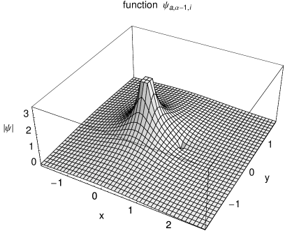
Figure 2: Function $\psi_{a,\alpha-1,\mathrm{i}}$ from the deficiency subspace for the values of parameters $\alpha=1/3$, $\beta=2/3$, $\rho=1$.

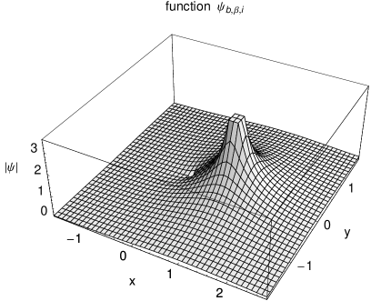
Figure 3: Function $\psi_{b,\beta,\mathrm{i}}$ from the deficiency subspace for the values of parameters $\alpha=1/3$, $\beta=2/3$, $\rho=1$.

Formula (V) is well suited for numerical computations. To give the reader an idea about the behavior of $\psi_{u,\nu,z}$ we have plotted $|\psi_{a,\alpha-1,\mathrm{i}}|$ in Fig. 2 and $|\psi_{b,\beta,\mathrm{i}}|$ in Fig. 3, with $\alpha=1/3$, $\beta=2/3$ and $\rho=1$. Note that the former function vanishes in the vortex $b$ while the latter one vanishes in the vortex $a$.

VI The Krein’s formula

We would like to emphasize once more that we are using two unitarily equivalent formulations. The operators $H^{\pm}$, $H_{0}$ are respectively associated to the quadratic forms (20) and (17). Let $U$ be the unitary operator in $L^{2}(\mathbb{R}^{2},\,\mathrm{d}^{2}x)$ acting as $U\varphi=\exp(\mathrm{i}\alpha\theta_{a}+\mathrm{i}\beta\theta_{b})\varphi$. The Green function (19) corresponds to the operator $H=UH_{0}U^{-1}$ defined by the boundary conditions on the cut (18).

Set

$$f_{u,\nu,z}=\Big{(}\sqrt{-z}\Big{)}^{\left|\nu\right|}\psi_{u,\nu,z}.$$ (49)

Let us enumerate the basis $\{f_{a,\alpha-1,z},f_{a,\alpha,z},f_{b,\beta-1,z},f_{b,\beta,z}\}$ in $\mathcal{N}(z)$ as $\{f_{z}^{1},f_{z}^{2},f_{z}^{3},f_{z}^{4}\}$ (in this order). Set $\widetilde{f}_{z}^{j}=U^{-1}f_{z}^{j}$, $R_{z}=(H_{0}-z)^{-1}$, $R_{z}^{\pm}=(H^{\pm}-z)^{-1}$. According to the Krein’s formula

$$R_{z}^{\pm}-R_{z}=\sum_{j,\,k}(M_{z}^{\pm})^{j,k}\,\widetilde{f}_{z}^{j}\langle\widetilde{f}_{\overline{z}}^{k},\cdot\rangle$$ (50)

or, in terms of Green functions,

$$\mathcal{G}_{z}^{\pm}(x,x_{0})=\mathcal{G}_{z}(x,x_{0})+\sum_{j,\,k}(M_{z}^{\pm})^{j,k}\,f_{z}^{j}(x)\,\overline{f_{\overline{z}}^{k}(x_{0})}\,,$$ (51)

where $M_{z}^{\pm}$ is a holomorphic matrix-valued function defined on $\mathbb{C}\setminus\mathbb{R}$.

An operator-valued function $R_{z}^{\pm}$ constructed this way will be the resolvent of a selfadjoint operator if and only if it satisfies [13, Chp. 5.2]

$$\forall z\in\mathbb{C}\setminus\mathbb{R},\textrm{ }(R_{z}^{\pm})^{*}=R_{\overline{z}}^{\pm}$$ (52)

and (the Hilbert identity)

$$\forall z,w\in\mathbb{C}\setminus\mathbb{R},\textrm{ }R_{z}^{\pm}-R_{w}^{\pm}=(z-w)R_{z}^{\pm}R_{w}^{\pm}\,$$ (53)

(it follows from (50) that $\operatorname{Ker}R_{z}^{\pm}=\{0\}$ for all $z\in\mathbb{C}\setminus\mathbb{R}$). Let us analyze conditions (52) and (53). It is straightforward to see that (52) is satisfied if and only if

$$M_{z}^{*}=M_{\overline{z}}.$$ (54)

In equality (58) below we shall show that

$$\forall z,w\in\mathbb{C}\setminus\mathbb{R},\,\forall j,\textrm{ }\widetilde{f}_{w}^{j}+(z-w)R_{z}\widetilde{f}_{w}^{j}=\widetilde{f}_{z}^{j}.$$

With the aid of this identity it is just an easy computation to show that (53) is equivalent to the condition

$$\forall z,w\in\mathbb{C}\setminus\mathbb{R},\textrm{ }M_{z}-M_{w}=(z-w)\,M_{z}P(\overline{z},w)\,M_{w}\,,$$ (55)

where $P(z,w)$ is the $4\times 4$ matrix of scalar products,

$$P(z,w)^{j,k}=\langle f_{z}^{j},f_{w}^{k}\rangle.$$

Equality (55) was presented in Ref. 14 and was applied to problems similar to ours for example in Refs. 15 and 3.

According to formula (36) and definition (37) of $\psi_{u,\nu,z}(x)$ we have

$$\mathcal{G}_{z}(x,x_{0}) = \frac{\sin(\pi\,\alpha)}{2\pi^{2}}\frac{\Gamma(\alpha)}{1-\alpha}\left(\frac{\sqrt{-z}\,r_{0a}}{2}\right)^{\!1-\alpha}\mathrm{e}^{-\mathrm{i}(\alpha-1)\theta_{0a}}\psi_{a,\alpha-1,z}(x)$$ (56)

$$+\,\frac{\sin(\pi\,\alpha)}{2\pi^{2}}\frac{\Gamma(1-\alpha)}{\alpha}\left(\frac{\sqrt{-z}\,r_{0a}}{2}\right)^{\!\alpha}\mathrm{e}^{-\mathrm{i}\,\alpha\,\theta_{0a}}\,\psi_{a,\alpha,z}(x)+O(r_{0a})$$

for $r_{0a}\downarrow 0$. Using this asymptotic behavior and the Hilbert identity written in terms of Green functions,

$$(z-w)\int_{\mathbb{R}^{2}}\mathcal{G}_{z}(x,y)\,\mathcal{G}_{w}(y,x_{0})\,\mathrm{d}^{2}y=\mathcal{G}_{z}(x,x_{0})-\mathcal{G}_{w}(x,x_{0})\,,$$

we obtain an equality valid for $u=a$, namely

$$(z-w)\Big{(}\sqrt{-w}\Big{)}^{\left|\nu\right|}\int_{\mathbb{R}^{2}}\mathcal{G}_{z}(x,y)\psi_{u,\nu,w}(y)\,\mathrm{d}^{2}y=\Big{(}\sqrt{-z}\Big{)}^{\left|\nu\right|}\psi_{u,\nu,z}(x)-\Big{(}\sqrt{-w}\Big{)}^{\left|\nu\right|}\psi_{u,\nu,w}(x)\,.$$ (57)

This means that

$$\psi_{u,\nu,w}+(z-w)(H-z)^{-1}\psi_{u,\nu,w}=\left(\frac{\sqrt{-z}}{\sqrt{-w}}\right)^{\!\left|\nu\right|}\psi_{u,\nu,z}$$

for $\nu\in\{\alpha-1,\alpha\}$ and $u=a$. The same argument naturally applies also to the vortex $u=b$. Using notation (49) we find that

$$f_{u,\nu,w}+(z-w)(H-z)^{-1}f_{u,\nu,w}=f_{u,\nu,z}$$ (58)

holds true for all $w,z\in\mathbb{C}\setminus\mathbb{R}$.

We wish to compute the $4\times 4$ matrix of scalar products $P(z,w).$ Using (34) and applying the asymptotic behavior (56) once more, this time to equality (57), we find that the integral

$$\int_{\mathbb{R}^{2}}\overline{\psi_{v,\mu,z}(y)}\,\psi_{u,\nu,w}(y)\,\mathrm{d}^{2}y$$

equals the coefficient standing at

$$\frac{\sin(\pi\left|\mu\right|)}{2\pi^{2}}\frac{\Gamma(1-\left|\mu\right|)}{\left|\mu\right|}\Big{(}\frac{r_{v}}{2}\Big{)}^{\left|\mu\right|}\mathrm{e}^{\mathrm{i}\,\mu\,\theta_{v}}$$

when taking the asymptotic expansion of the expression

$$\frac{1}{\overline{z}-w}\left(\frac{1}{\big{(}\sqrt{-w}\big{)}^{\left|\nu\right|}}\,\psi_{u,\nu,\overline{z}}(x)-\frac{1}{\big{(}\sqrt{-\overline{z}}\big{)}^{\left|\nu\right|}}\,\psi_{u,\nu,w}(x)\right)$$

for $x\rightarrow v$, i.e., $r_{v}\downarrow 0$. In virtue of (V) and (43) we get

$$\int_{\mathbb{R}^{2}}\overline{\psi_{a,\mu,z}(y)}\,\psi_{a,\nu,w}(y)\,\mathrm{d}^{2}y$$

$$\qquad\quad=-2\pi\,\frac{1}{\overline{z}-w}\left(\left(\frac{\sqrt{-\overline{z}}}{\sqrt{-w}}\right)^{\!\left|\nu\right|}\mathcal{T}_{\mu,\nu}(\alpha,\beta;\overline{z})-\left(\frac{\sqrt{-w}}{\sqrt{-\overline{z}}}\right)^{\!\left|\mu\right|}\mathcal{T}_{\mu,\nu}(\alpha,\beta;w)\right)$$

and

$$\int_{\mathbb{R}^{2}}\overline{\psi_{a,\mu,z}(y)}\,\psi_{b,\nu,w}(y)\,\mathrm{d}^{2}y$$

$$\qquad\quad=\,2\pi\,\frac{1}{\overline{z}-w}\left(\left(\frac{\sqrt{-\overline{z}}}{\sqrt{-w}}\right)^{\!\left|\nu\right|}\mathcal{S}_{\nu,\mu}(\alpha,\beta;\overline{z})-\left(\frac{\sqrt{-w}}{\sqrt{-\overline{z}}}\right)^{\!\left|\mu\right|}\mathcal{S}_{\nu,\mu}(\alpha,\beta;w)\right).$$

In particular,

$$\int_{\mathbb{R}^{2}}\left|\psi_{a,\nu,z}(x)\right|^{2}\,\,\mathrm{d}^{2}x=-\frac{2\pi}{\operatorname{Im}(z)}\,\operatorname{Im}\!\left(\left(\frac{\sqrt{-z}}{\sqrt{-\overline{z}}}\right)^{\!\left|\nu\right|}\mathcal{T}_{\nu,\nu}(\alpha,\beta;z)\right)\,.$$

This means that, when passing to functions $\{f_{z}^{j}\}$ instead of $\{\psi_{u,\nu,z}\}$,

$$(\overline{z}-w)\,P(z,w)$$

$$\textrm{ }=-2\pi\left(\begin{matrix}\big{(}\sqrt{-\overline{z}}\big{)}^{2-2\alpha}\mathcal{T}_{\alpha-1,\alpha-1}(\alpha,\beta;\overline{z})&\sqrt{-\overline{z}}\,\mathcal{T}_{\alpha,\alpha-1}(\alpha,\beta;\overline{z})\\ \sqrt{-\overline{z}}\,\mathcal{T}_{\alpha-1,\alpha}(\alpha,\beta;\overline{z})&\big{(}\sqrt{-\overline{z}}\big{)}^{2\alpha}\mathcal{T}_{\alpha,\alpha}(\alpha,\beta;\overline{z})\\ -\big{(}\sqrt{-\overline{z}}\big{)}^{2-\alpha-\beta}\mathcal{S}_{\alpha-1,\beta-1}(\beta,\alpha;\overline{z})&-\big{(}\sqrt{-\overline{z}}\big{)}^{1+\alpha-\beta}\mathcal{S}_{\alpha,\beta-1}(\beta,\alpha;\overline{z})\\ -\big{(}\sqrt{-\overline{z}}\big{)}^{1-\alpha+\beta}\mathcal{S}_{\alpha-1,\beta}(\beta,\alpha;\overline{z})&-\big{(}\sqrt{-\overline{z}}\big{)}^{\alpha+\beta}\mathcal{S}_{\alpha,\beta}(\beta,\alpha;\overline{z})\end{matrix}\right.$$

(59)

$$\quad\left.\begin{matrix}-\big{(}\sqrt{-\overline{z}}\big{)}^{2-\alpha-\beta}\mathcal{S}_{\beta-1,\alpha-1}(\alpha,\beta;\overline{z})&-\big{(}\sqrt{-\overline{z}}\big{)}^{1-\alpha+\beta}\mathcal{S}_{\beta,\alpha-1}(\alpha,\beta;\overline{z})\\ -\big{(}\sqrt{-\overline{z}}\big{)}^{1+\alpha-\beta}\mathcal{S}_{\beta-1,\alpha}(\alpha,\beta;\overline{z})&-\big{(}\sqrt{-\overline{z}}\big{)}^{\alpha+\beta}\mathcal{S}_{\beta,\alpha}(\alpha,\beta;\overline{z})\\ \big{(}\sqrt{-\overline{z}}\big{)}^{2-2\beta}\mathcal{T}_{\beta-1,\beta-1}(\beta,\alpha;\overline{z})&\sqrt{-\overline{z}}\,\mathcal{T}_{\beta,\beta-1}(\beta,\alpha;\overline{z})\\ \sqrt{-\overline{z}}\,\mathcal{T}_{\beta-1,\beta}(\beta,\alpha;\overline{z})&\big{(}\sqrt{-\overline{z}}\big{)}^{2\beta}\mathcal{T}_{\beta,\beta}(\beta,\alpha;\overline{z})\end{matrix}\right)$$

$$-\,(\overline{z}\leftrightarrow w)\,.$$

The Green functions $\mathcal{G}_{z}^{\pm}(x,x_{0})$ should satisfy the corresponding boundary conditions in each variable $x$, $x_{0}$. Let us first consider the case of $H^{+}$. Recall that the boundary conditions which determine the domain of $H^{+}$ are $\Phi_{2}^{-1}=\Phi_{1}^{0}=0$ (see (21)). Let us check the asymptotic behavior of $\mathcal{G}_{z}^{\pm}(x,x_{0})$ for $x_{0}\rightarrow a$. Asymptotic behavior of $\mathcal{G}_{z}(x,x_{0})$ is given in (56) and asymptotic behavior of $f_{z}^{j}(x_{0})$ follows from (V) and (43) jointly with definition (49). The condition $\Phi_{1}^{0}=0$ means that the coefficient standing at $(r_{0a}/2)^{-\alpha}\exp(-\mathrm{i}\alpha\theta_{0a})$ vanishes. This term occurs only in the asymptotic expansion of $f_{z}^{2}(x_{0})$ and so

$$\sum_{j}(M_{z}^{+})^{j,2}\,f_{z}^{j}(x)=0\,.$$

The set of functions $\{f_{z}^{j}\}$ is linearly independent and thus we get a condition on the matrix $M_{z}^{+}$: $(M_{z}^{+})^{j,2}=0$ for all $j$. Considering the limit $x_{0}\rightarrow b$ one similarly derives the condition $(M_{z}^{+})^{j,4}=0$. In view of (54) one obtains more, namely

$$(M_{z}^{+})^{j,k}=0\quad\textrm{whenever }j=2,4\textrm{ or }k=2,4.$$ (60)

Let us denote by $M_{z}^{+,\textrm{red }}$ the reduced $2\times 2$ matrix obtained by omitting the vanishing rows and columns, i.e.,

$$M_{z}^{+,\textrm{red }}=\begin{pmatrix}(M_{z}^{+})^{1,1}&(M_{z}^{+})^{1,3}\\ (M_{z}^{+})^{3,1}&(M_{z}^{+})^{3,3}\end{pmatrix}.$$

The condition $\Phi_{2}^{-1}=0$ for $x_{0}\rightarrow a$ means that the coefficient standing at $(r_{0a}/2)^{1-\alpha}\exp\!\big{(}-\mathrm{i}(\alpha-1)\theta_{0a}\big{)}$ vanishes. Using (60) we get

$$\frac{\sin(\pi\,\alpha)}{2\pi^{2}}\frac{\Gamma(\alpha)}{1-\alpha}f_{z}^{1}(x)+\sum_{j}f_{z}^{j}(x)\bigg{(}-(M_{z}^{+})^{j,1}\,\frac{\sin(\pi\,\alpha)}{\pi}\frac{\Gamma(\alpha)}{1-\alpha}$$

$$\textrm{ }\times\,\big{(}\sqrt{-z}\,\big{)}^{2(1-\alpha)}\,\mathcal{T}_{\alpha-1,\alpha-1}(\alpha,\beta;z)$$

$$+\,(M_{z}^{+})^{j,3}\,\frac{\sin(\pi\,\alpha)}{\pi}\frac{\Gamma(\alpha)}{1-\alpha}\big{(}\sqrt{-z}\,\big{)}^{2-\alpha-\beta}\,\mathcal{S}_{\alpha-1,\beta-1}(\beta,\alpha;z)\bigg{)}=0.$$

This is equivalent to the couple of equations

$$\frac{1}{2\pi}-(M_{z}^{+})^{1,1}\big{(}\sqrt{-z}\,\big{)}^{2(1-\alpha)}\,\mathcal{T}_{\alpha-1,\alpha-1}(\alpha,\beta;z)\hskip 120.00018pt$$

$$+\,(M_{z}^{+})^{1,3}\big{(}\sqrt{-z}\,\big{)}^{2-\alpha-\beta}\,\mathcal{S}_{\alpha-1,\beta-1}(\beta,\alpha;z) = 0,$$

$$-\,(M_{z}^{+})^{3,1}\big{(}\sqrt{-z}\,\big{)}^{2(1-\alpha)}\,\mathcal{T}_{\alpha-1,\alpha-1}(\alpha,\beta;z)\hskip 120.00018pt$$

$$+\,(M_{z}^{+})^{3,3}\big{(}\sqrt{-z}\,\big{)}^{2-\alpha-\beta}\,\mathcal{S}_{\alpha-1,\beta-1}(\beta,\alpha;z) = 0.$$

Analogously, another two equations are obtained when considering the limit $x_{0}\rightarrow b$, namely

$$\frac{1}{2\pi}-(M_{z}^{+})^{3,3}\big{(}\sqrt{-z}\,\big{)}^{2(1-\beta)}\,\mathcal{T}_{\beta-1,\beta-1}(\beta,\alpha;z)\hskip 120.00018pt$$

$$+\,(M_{z}^{+})^{3,1}\big{(}\sqrt{-z}\,\big{)}^{2-\alpha-\beta}\,\mathcal{S}_{\beta-1,\alpha-1}(\alpha,\beta;z) = 0,$$

$$-\,(M_{z}^{+})^{1,3}\big{(}\sqrt{-z}\,\big{)}^{2(1-\beta)}\,\mathcal{T}_{\beta-1,\beta-1}(\beta,\alpha;z)\hskip 120.00018pt$$

$$+\,(M_{z}^{+})^{1,1}\big{(}\sqrt{-z}\,\big{)}^{2-\alpha-\beta}\,\mathcal{S}_{\beta-1,\alpha-1}(\alpha,\beta;z) = 0.$$

The four equations can be jointly rewritten in the matrix form,

$$M_{z}^{+,\textrm{red }}$$ (61)

$$=\frac{1}{2\pi}\begin{pmatrix}\big{(}\sqrt{-z}\big{)}^{2-2\alpha}\mathcal{T}_{\alpha-1,\alpha-1}(\alpha,\beta;z)&-\big{(}\sqrt{-z}\big{)}^{2-\alpha-\beta}\mathcal{S}_{\beta-1,\alpha-1}(\alpha,\beta;z)\\ -\big{(}\sqrt{-z}\big{)}^{2-\alpha-\beta}\mathcal{S}_{\alpha-1,\beta-1}(\beta,\alpha;z)&\big{(}\sqrt{-z}\big{)}^{2-2\beta}\mathcal{T}_{\beta-1,\beta-1}(\beta,\alpha;z)\end{pmatrix}^{-1}.$$

It is straightforward to verify that the derived matrix $M_{z}^{+}$ actually obeys conditions (54) and (55). The former one follows from the equalities

$$\overline{\mathcal{T}_{\mu,\nu}(\alpha,\beta;z)}=\mathcal{T}_{\mu,\nu}(\alpha,\beta;\overline{z}),\textrm{ }\overline{\mathcal{S}_{\mu,\nu}(\alpha,\beta;z)}=\mathcal{S}_{\mu,\nu}(\alpha,\beta;\overline{z}),$$

and

$$\mathcal{T}_{\mu,\nu}(\alpha,\beta;z)=\mathcal{T}_{\nu,\mu}(\alpha,\beta;z),\textrm{ }\mathcal{S}_{\mu,\nu}(\alpha,\beta;z)=\mathcal{S}_{\nu,\mu}(\beta,\alpha;z).$$

The latter one follows from the form of $P(z,w)$ given in (59). In fact, (59) and (61) jointly imply

$$(\overline{z}-w)\,P(z,w)^{\textrm{red}}=\big{(}M_{w}^{+,\textrm{red}}\big{)}^{-1}-\big{(}M_{\overline{z}}^{+,\textrm{red}}\big{)}^{-1}.$$

The other component of the Pauli operator, $H^{-}$, can be treated similarly. The boundary conditions read $\Phi_{1}^{-1}=\Phi_{2}^{0}=0$ (see (22)). The condition $\Phi_{1}^{-1}=0$ for $x_{0}\rightarrow a$ means that the coefficient standing at $(r_{0a}/2)^{-1+\alpha}\exp\!\big{(}-\mathrm{i}(\alpha-1)\theta_{0a}\big{)}$ vanishes. Hence

$$\sum_{j}(M_{z}^{-})^{j,1}\,f_{z}^{j}(x)=0\,,$$

or equivalently, $(M_{z}^{-})^{j,1}=0$. Similarly for $x_{0}\rightarrow 0$ we derive that $(M_{z}^{-})^{j,3}=0$, hence

$$(M_{z}^{-})^{j,k}=0\quad\textrm{whenever }j=1,3\textrm{ or }k=1,3.$$ (62)

Set

$$M_{z}^{-,\textrm{red }}=\begin{pmatrix}(M_{z}^{-})^{2,2}&(M_{z}^{-})^{2,4}\\ (M_{z}^{-})^{4,2}&(M_{z}^{-})^{4,4}\end{pmatrix}.$$

The condition $\Phi_{2}^{0}=0$ for $x_{0}\rightarrow a$ means that the coefficient standing at $(r_{0a}/2)^{\alpha}\exp(-\mathrm{i}\alpha\theta_{0a})$ vanishes. Using (62) we get

$$\frac{\sin(\pi\,\alpha)}{2\pi^{2}}\frac{\Gamma(1-\alpha)}{\alpha}f_{z}^{2}(x)+\sum_{j}f_{z}^{j}(x)\bigg{(}-(M_{z}^{+})^{j,2}\,\frac{\sin(\pi\,\alpha)}{\pi}\frac{\Gamma(1-\alpha)}{\alpha}$$

$$\qquad\times\,\big{(}\sqrt{-z}\,\big{)}^{2\,\alpha}\,\mathcal{T}_{\alpha,\alpha}(\alpha,\beta;z)$$

$$\quad+\,(M_{z}^{+})^{j,4}\,\frac{\sin(\pi\,\alpha)}{\pi}\frac{\Gamma(1-\alpha)}{\alpha}\big{(}\sqrt{-z}\,\big{)}^{\alpha+\beta}\,\mathcal{S}_{\alpha,\beta}(\beta,\alpha;z)\bigg{)}=0.$$

This is equivalent to the couple of equations

$$\frac{1}{2\pi}-(M_{z}^{-})^{2,2}\big{(}\sqrt{-z}\,\big{)}^{2\alpha}\,\mathcal{T}_{\alpha,\alpha}(\alpha,\beta;z)+(M_{z}^{-})^{2,4}\big{(}\sqrt{-z}\,\big{)}^{\alpha+\beta}\,\mathcal{S}_{\alpha,\beta}(\beta,\alpha;z) = 0,$$

$$-\,(M_{z}^{-})^{4,2}\big{(}\sqrt{-z}\,\big{)}^{2\alpha}\,\mathcal{T}_{\alpha,\alpha}(\alpha,\beta;z)+(M_{z}^{-})^{4,4}\big{(}\sqrt{-z}\,\big{)}^{\alpha+\beta}\,\mathcal{S}_{\alpha,\beta}(\beta,\alpha;z) = 0.$$

For $x_{0}\rightarrow b$ one derives other two equations,

$$\frac{1}{2\pi}-(M_{z}^{-})^{4,4}\big{(}\sqrt{-z}\,\big{)}^{2\beta}\,\mathcal{T}_{\beta,\beta}(\beta,\alpha;z)+(M_{z}^{-})^{4,2}\big{(}\sqrt{-z}\,\big{)}^{\alpha+\beta}\,\mathcal{S}_{\beta,\alpha}(\alpha,\beta;z) = 0,$$

$$-(M_{z}^{-})^{2,4}\big{(}\sqrt{-z}\,\big{)}^{2\beta}\,\mathcal{T}_{\beta,\beta}(\beta,\alpha;z)+(M_{z}^{-})^{2,2}\big{(}\sqrt{-z}\,\big{)}^{\alpha+\beta}\,\mathcal{S}_{\beta,\alpha}(\alpha,\beta;z) = 0.$$

Jointly the four equations mean that

$$M_{z}^{-,\textrm{red }}=\frac{1}{2\pi}\begin{pmatrix}\big{(}\sqrt{-z}\big{)}^{2\alpha}\mathcal{T}_{\alpha,\alpha}(\alpha,\beta;z)&-\big{(}\sqrt{-z}\big{)}^{\alpha+\beta}\mathcal{S}_{\beta,\alpha}(\alpha,\beta;z)\\ -\big{(}\sqrt{-z}\big{)}^{\alpha+\beta}\mathcal{S}_{\alpha,\beta}(\beta,\alpha;z)&\big{(}\sqrt{-z}\big{)}^{2\beta}\mathcal{T}_{\beta,\beta}(\beta,\alpha;z)\end{pmatrix}^{-1}.$$ (63)

Let us note that the inverted matrices on the RHS of (61) and (63) are actually well defined. This is because the matrices in question depend on $z$ analytically in the domain $\mathbb{C}\setminus\mathbb{R}_{+}$ and tend exponentially fast to invertible diagonal matrices for $\operatorname{Re}\sqrt{-z}\rightarrow+\infty$ as one can easily deduce from the discussion of the formula (V) related to the convergence of the series (37a) and from the form of matrix entries (44) and (47).

VII Concluding remarks

Having a formula for the Green function $\mathcal{G}_{z}^{\pm}(x,x_{0})$ it would be, of course, desirable to use it for a more detailed analysis of the Pauli operator, first of all for its spectral analysis. This aim would assume, however, a more detailed analysis of the functions $\mathcal{S}_{\omega,\nu}(\alpha,\beta;z)$ and $\mathcal{T}_{\omega,\nu}(\alpha,\beta;z)$. In particular, it would be important to know what happens in the limit $\operatorname{Re}\sqrt{-z}\rightarrow 0$, i.e., when $z$ approaches $\lambda\in\mathbb{R}_{+}$ from the upper or lower half-plane. Recall that both $\mathcal{S}_{\omega,\nu}(\alpha,\beta;z)$ and $\mathcal{T}_{\omega,\nu}(\alpha,\beta;z)$ are expressed as infinite series whose convergence is guaranteed for $\operatorname{Re}\sqrt{-z}>0$. Our first attempts in this direction suggest that such an analysis might be rather complex and should be considered as an independent problem in its own right.

Figure captions

FIGURE 1. Geometrical arrangement. Choice of the cuts $L_{a}$, $L_{b}$ and choice of the angle variables $\theta_{a}$, $\theta_{b}$.

FIGURE 2. Function $\psi_{a,\alpha-1,\mathrm{i}}$ from the deficiency subspace for the values of parameters $\alpha=1/3$, $\beta=2/3$, $\rho=1$.

FIGURE 3. Function $\psi_{b,\beta,\mathrm{i}}$ from the deficiency subspace for the values of parameters $\alpha=1/3$, $\beta=2/3$, $\rho=1$.