An alternative inference tool to total probability formula and its applications

Abstract

An alternative inference tool for using prior information to calculate marginal distribution function in the Bayesian statistics is suggested. A few applications of this new tool are given.

1 Introduction

Total probability and Bayes formula are two basic tools for using prior information in the Bayesian statistics. In this paper we introduce an alternative tool for using prior information. This new toold enables us to improve some traditional results in statistical inference. However, as far as the authors know, there is no work on this subject, except [1]. The results of this paper can be extended to other branches of probability and statistics.

In Section 2 total probability formula based on median is defined and its basic properties are proved. A few applications of this new tool are given in Section 3. All computations and plots are done using the S-PLUS software system.

2 Total probability formula based on median

Let $X$ be a continuous random variable with distribution function $F_{X|\nu}(x|\nu)$, which depends on parameter $\nu$ with known and continuous density function $\pi(.)$. The marginal distribution function $X$ can be calculated by total probability formula, i.e.

$$F_{X}(x)=\int_{-\infty}^{\infty}F_{X|\nu}(x|\nu)\;\pi(\nu)\;\mbox{d}\nu$$ (1)

Therefore $F_{X}$ is a weighted mean of $F_{X|\nu}$, i.e., $F_{X}$ is the expected value of $F_{X|\nu}$ over $\pi$. Our idea for the following definition is similar to (1).

Definition 1

Let $X$ have a distribution function depending on parameter $\nu$, where $\nu$ has a density function $\pi(.)$. The marginal distribution function of $X$ based on median, $\widetilde{F}_{X}(x)$, is defined as the median of $F_{X|\nu}(x|v)$ over $\pi$.

We recall that median is robust with respect to outlier data, but mean is not. To simplify calculations of $\widetilde{F}_{X}(x)$, we use definition of median in statistics. That is we calculate $\widetilde{F}_{X}(x)$ by solving the following equation

$$F_{F_{X|\nu}(x|\nu)}(\widetilde{F}_{X}(x))=\frac{1}{2},\;\;\mbox{~{}or equivalently~{}}\;\;P(F_{X|\nu}(x|\nu)\leq\widetilde{F}_{X}(x))=\frac{1}{2}.$$ (2)

The following theorem states an important property of $\widetilde{F}_{X}(x)$.

Theorem 1

$\widetilde{F}_{X}(x)$ is a non-decreasing and continuous function of $x$.

Proof: Let $x_{1}<x_{2}$. For $i=1,2$, take

$$k_{i}=\widetilde{F}_{X}(x_{i})\mbox{~{}~{}~{}and~{}~{}~{}}Y_{i}=F_{X|\nu}(x_{i}|\nu).$$

Then using 2 we have

$$P(Y_{1}\leq k_{1})=P(Y_{2}\leq k_{2})=\frac{1}{2}.$$

We also have

$$Y_{1}\leq Y_{2}.$$

Therefore,

$$P(Y_{1}\leq k_{1})=P(Y_{2}\leq k_{2})\leq P(Y_{1}\leq k_{2}),$$

i.e. $k_{1}\leq k_{2}$ or equivalently $\widetilde{F}_{X}(x)$ is non-decreasing.
If $\widetilde{F}_{X}(x)$ is a non-decreasing function, then

$$\widetilde{F}_{X}(x_{-})=\lim_{t\uparrow x}\widetilde{F}_{X}(t)\;\;\mbox{and}\;\;\tilde{F}_{X}(x_{+})=\lim_{t\downarrow x}\widetilde{F}_{X}(t)$$

exist and are finite (e.g. [2]).

Further, $F_{X|\nu}(x|\nu)$ is continuous with respect to $x$, and so

$$P(F_{X|\nu}(x_{-}|\nu)\leq\tilde{F}_{X|\nu}(x_{-}))=P(F_{X|\nu}(x|\nu)\leq\widetilde{F}_{X}(x_{-})),$$

$$P(F_{X|\nu}(x_{+}|\nu)\leq\widetilde{F}_{X}(x_{+}))=P(F_{X|\nu}(x|\nu)\leq\widetilde{F}_{X}(x_{+})).$$

And by (2) we have

$$P(F_{X|\nu}(x|\nu)\leq\widetilde{F}_{X}(x_{-})) = P(F_{X|\nu}(x|\nu)\leq\widetilde{F}_{X}(x))$$ (3)

$$= P(F_{X|\nu}(x|\nu)\leq\widetilde{F}_{X}(x_{+})).$$

If $Y=F_{X|\nu}(x|\nu)$ has an increasing distribution function, then

$$\widetilde{F}_{X}(x_{-})=\widetilde{F}_{X}(x)=\widetilde{F}_{X}(x_{+})$$

and by (3) $\widetilde{F}_{X}(x)$ is continuous.

On the other hand $\widetilde{F}_{X}(x)$ is the median of $Y$, $0\leq Y\leq 1$, and so

$$0\leq\widetilde{F}_{X}(x)\leq 1.$$

Also, by Theorem 1, $\widetilde{F}_{X}(+\infty)$ and $\widetilde{F}_{X}(-\infty)$ exist as

$$\lim_{t\uparrow+\infty}\widetilde{F}_{X}(t)\;\;\mbox{and}\;\;\lim_{t\downarrow-\infty}\widetilde{F}_{X}(t)$$

respectively. Therefore $\widetilde{F}_{X}(x)$ is a distribution function if

$$\tilde{F}_{X}(+\infty)=1\;\;\mbox{and}\;\;\widetilde{F}_{X}(-\infty)=0.$$

Example 1

Let ${X}$ be exponentially distributed, i.e.

$$F_{X|\nu}(x|\nu)=1-e^{-\nu x},\;\;x>0$$

and assume $\pi(\nu)=1,\;0<\nu\leq 1$.

In this example we can calculate $\widetilde{F}_{X}$ exactly by equation (2) as follows

$$P(1-e^{-\nu x}\leq\widetilde{F}_{X}(x))=\frac{1}{2}$$

$$\Longleftrightarrow P(\nu\leq\frac{-1}{x}\ \ln(1-\widetilde{F}_{X}(x)))=\frac{1}{2}$$

$$\Longleftrightarrow \frac{-1}{x}\ \ln(1-\widetilde{F}_{X}(x))=\frac{1}{2}$$

$$\Longleftrightarrow \widetilde{F}_{X}(x)=1-e^{-x/2},\;x>0.$$

It can be shown that $\widetilde{F}_{X}$ is a distribution function. Moreover,

$$F_{X}(x)=1+\frac{1}{x}(e^{-x}-1),\;x>0.$$

In some problems we cannot calculate $\widetilde{F}_{X}$ exactly. But, we can approximate it in the two following cases.

Algorithm M1: When $F_{X|\nu}(x|\nu)$ has an analytic form, but we cannot calculate $\widetilde{F}_{X}$ analytically.

1. Fix $x$ (say $x_{0}$)

2. Generate $K$ sample for $\nu$ by using $\pi(\nu)$ (say $\nu_{k},\;k=1\cdots,K)$

3. Calculate the sample median of
   $F_{X}(x_{0};\nu_{1}),\cdots,F_{X}(x_{0};\nu_{K})$

4. Repeat from step 1 with another choice of $x$.

Algorithm M2: When $F_{X|\nu}(x|\nu)$ has not an analytic form.

1. Fix $x$ (say $x_{0}$)

2. Generate $K$ sample for $\nu$ by using $\pi(\nu)$ (say $\nu_{k},\;k=1\cdots,K)$

3. Generate $L$ sample for $X|\nu_{k}$ for each $k(=1,\cdots,K)$
   (say $(x_{1}|\nu_{1},\cdots,x_{L}|\nu_{1})\cdots(x_{1}|\nu_{K},\cdots,x_{L}|\nu_{K})$)

4. Calculate the empirical distribution function of $X|\nu_{k}$ for each $k(=1,\cdots,K)$ (based on generated samples in the previous step)

5. Calculate the sample median of empirical distribution functions in step 4 and repeat from step 1 with another choice of $x$.

Remark 1 We can approximate $F_{X}$ by algorithms similar to M1 and M2 (are called B1 and B2 corresponding to M1 and M2).
Figure 1, shows the graphs of $\widetilde{F}_{X}$, $F_{X}$, and their approximations for Example 1.

Example 2

Let ${X}$ be exponentially distributed, (similar Example 1) i.e.

$$F_{X|\nu}(x|\nu)=1-e^{-\nu x},\;\;x>0$$

but here

$$\pi(\nu)=e^{-\nu},\;\nu>0.$$

In this case

$$\widetilde{F}_{X}(x)=1-e^{x\ln(1/2)},\;x>0,$$

is a distribution function and

$$F_{X}(x)=1-\frac{1}{x+1},\;x>0.$$

Figure 2 shows their graphs.

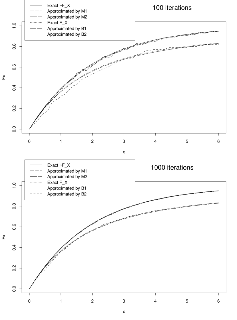
Figure 1: Graphs of $\widetilde{F}_{X}$, $F_{X}$, and their approximations in Example 1 for $K=100,1000$

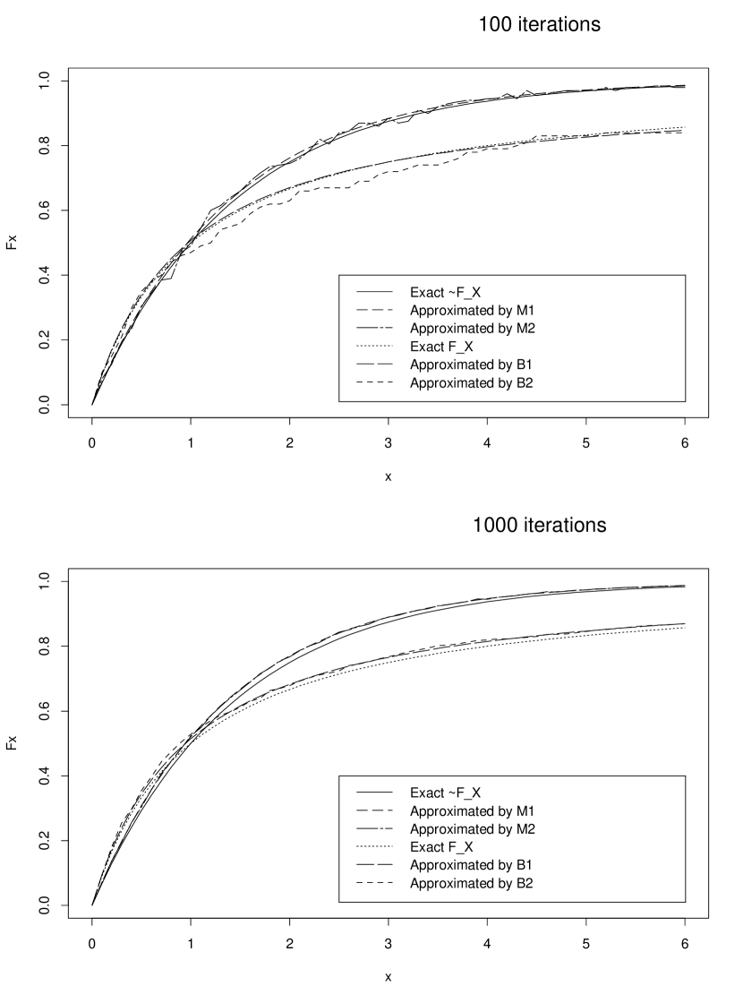
Figure 2: Graphs of $\widetilde{F}_{X}$, $F_{X}$, and their approximations in Example 2 for $K=100,1000$

3 Hypothesis Testing

In this section we introduce a few applications of $\widetilde{F}_{X}$ to improve traditional results in statistical inference.

In the previous section we showed that $\widetilde{F}_{X}$ is a distribution function under a few conditions. If $\widetilde{F}_{X}$ depends on some unknown parameters we can apply classical methods in statistics to make inference about the unknown parameters. For example, uniformly most powerful (UMP) test can be calculated by Karlin-Robin theorem , or the most powerful (MP) test can be calculated by the following version of Neyman-Pearson lemma’s.

Lemma 1.1

Consider testing

$$\left\{{{H_{0}:\theta=\theta_{0}}\atop{H_{1}:\theta=\theta_{1}}}\right.,$$ (4)

where $\theta$ is an unknown parameter of $\widetilde{F}_{X}$ and $\theta_{0}$, $\theta_{1}$ are fixed known numbers. If $\widetilde{F}_{X}$ does not depend on any other unknown parameters under $H_{0}$ and $H_{1}$, then

$$\phi(x)=\left\{{{1\;\;\;\frac{d\widetilde{F}_{X}(x)}{dx}\mid_{\theta=\theta_{1}}>k\frac{d\widetilde{F}_{X}(x)}{dx}\mid_{\theta=\theta_{0}}}\atop{0\;\;\;\frac{d\widetilde{F}_{X}(x)}{dx}\mid_{\theta=\theta_{1}}<k\frac{d\widetilde{F}_{X}(x)}{dx}\mid_{\theta=\theta_{0}}}}\right.,$$ (5)

for some $k\geq 0$, is the MP test of its size for testing.

Proof: Let $\widetilde{F}_{X}(x)=\frac{d\widetilde{F}_{X}(x)}{dx}$. Then $\widetilde{F}_{X}(x)$ is a continuous density function which does not depend on any other unknown parameters under $H_{0}$ and $H_{1}$. Therefore by the Neyman-Pearson lemma (1.1) is the MP test of its size for testing (5).

Example 3

Consider testing

$$\left\{{{H_{0}:\mu=0}\atop{H_{1}:\mu<0}}\right..$$ (6)

based on an observation from a normal distribution $X\sim N(\mu,\sigma^{2})$.

If $\sigma^{2}$ is known, then the family of normal distribution has Monotone Likelihood Ratio (MLR) property and according to the Karlin-Robin theorem

$$\phi_{\sigma^{2}}(x)=\left\{{{1\;\;\;\;\;\;\;\frac{x}{\sigma}<z_{\alpha}}\atop{0\;\;\;\;\;\;\;\frac{x}{\sigma}>z_{\alpha}}}\right.,$$ (7)

is the Uniformly Most Powerful (UMP), of size $\alpha$ test function for 6, where $P(Z<z_{\alpha})=\alpha$ and $Z\sim N(0,1)$. But, if $\sigma^{2}$ is unknown, then the best test does not exist.

In the Bayesian approach, where $\sigma^{2}$ (variance) has a prior density function such as uniform or exponential (where defined in Examples 1 and  2 respectively), we can find marginal distribution functions $F_{X}$ and $\widetilde{F}_{X}$ which depends on $\mu$. Figure 3 shows the graphs of power functions of the tests based on $F_{X}$ and $\widetilde{F}_{X}$ for $\alpha=0.05$. We also plot the graph of power function of 7 for $\sigma=0.4,1$ (i.e. when $\sigma$ is known). The graphs show that the test based on $\widetilde{F}_{X}$ is better than the test based on $F_{X}$, when we use exponential prior for $\sigma^{2}$.

Moreover, we plot the graphs of power functions of the tests based on $F_{X}$ and $\widetilde{F}_{X}$ in the two cases of uniform and exponential prior distributions for $\sigma$ (standard deviation) in Figure 3. The result is incredible! The test based on $\widetilde{F}_{X}$ is much better than the test based on $F_{X}$.

Figure 3: The graphs of power functions when the variance has a uniform and exponential prior.

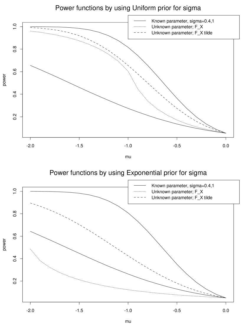
Figure 4: The graphs of power functions, when the standard deviation has a uniform and exponential prior.

4 Parameter estimation

Consider the case where the distribution of X depends on two parameters $\theta$ and $\nu$, i.e.,, we have $F_{X|\nu,\theta}(x|\nu,\theta)$. Then, we can define $F_{X|\theta}(x|\theta)$ and $\widetilde{F}_{X|\theta}(x|\theta)$ as in previous case. Then, by derivating them with respect to $x$, we can also define $f_{X|\theta}(x|\theta)$ and $\widetilde{f}_{X|\theta}(x|\theta)$. Assume now that we have a data set $x-1,\cdots,x_{N}$ where we assume its distribution to be $F_{X|\nu,\theta}(x|\nu,\theta)$ and where we have prior knowledge $\pi(\nu)$, and we want to estimate $\theta$ for this data set.

The classical MLE is defined by

$$\widehat{\theta}=\mathop{\mathrm{arg\,max}}_{\theta}\left\{L(\theta)=\prod_{i=1}^{N}f_{X|\theta}(x_{i}|\theta)\right\}$$ (8)

Similarly, based on our new criterion we propose the following

$$\widehat{\theta}=\mathop{\mathrm{arg\,max}}_{\theta}\left\{\widetilde{L}(\theta)=\prod_{i=1}^{N}\widetilde{f}_{X|\theta}(x_{i}|\theta)\right\}.$$ (9)

To show the relative performances of these two estimators, we

TO COMPLETE LATER

5 Conclusion

We introduced an alternative inference tool for using prior information $\pi(\nu)$ by defining a marginal function $\widetilde{F}_{X|\nu}(x|\nu)$ which is based on median in place of $F_{X|\nu}(x|\nu)$ which is the expected value of $\widetilde{F}_{X|\nu}(x|\nu)$ with respect to $\pi(\nu)$. We proved that $\widetilde{F}_{X|\nu}(x|\nu)$ is a non-decreasing and continuous function of $x$ and presented some of its applications and its performances in hypothesis testing and in parameter estimation.

References

(1)Mohammadpour, A. (2003) Fuzzy Parameter and Its Application in Hypothesis
Testing, Technical Report, School of Intelligent Systems, IPM,
Tehran, Iran.
(2)Rohatgi, V. K. (1976). An Introduction to Probability Theory and Mathematical Statistics. John Wiley and Sons, New York.