Properties of continuous Fourier extension
of the discrete cosine transform and
its multidimensional generalization

Abstract

A versatile method is described for the practical computation of the exact discrete Fourier transforms (DFT), both the direct and the inverse ones, of a continuous function $g$ given by its values $g_{j}$ at the points of a uniform grid ${\sf F}_{N}$ generated by conjugacy classes of elements of finite adjoint order $N$ in the fundamental region $F$ of compact semisimple Lie groups. The present implementation of the method is for the groups $SU(2)$, when ${\sf F}$ is reduced to a one-dimensional segment, and for $SU(2)\times SU(2)\cdots\times SU(2)$ in multidimensional cases. This simplest case turns out to be a version of the discrete cosine transform (DCT). Implementations, abbreviated as DGT for Discrete Group Transform, based on simple Lie groups of higher ranks, are considered separately.

DCT is often considered to be simply a specific type of the standard DFT. Here we show that the DCT is very different from the standard DFT when the properties of the continuous extensions of the two inverse discrete transforms from the discrete $t_{j}\in F_{N}$ to all points $t\in{\sf F}$ are studied. The following properties of the continuous extension of DCT (called CEDCT) are proven and exemplified.

Like the standard DFT, the DCT also returns the exact values of $\{g_{j}\}$ on the $N+1$ points of the grid. However, unlike the continuous extension of the standard DFT,

(a) the CEDCT function $f_{N}(t)$ closely approximates $g(t)$ between the points of the grid as well.

(b) For increasing $N$, the derivative of $f_{N}(t)$ converges to the derivative of $g(t)$.

(c) For CEDCT the principle of locality is valid.

Finally we use the continuous extension of the 2-dimensional DCT, $SU(2)\times SU(2)$, to illustrate its potential for interpolation as well as for the data compression of 2D images.

1 Introduction

The decomposition of functions integrable on a finite segment into Fourier series of trigonometric functions of one variable is a well known method (e.g. [1, 2]) whose theoretical and practical aspects have been thoroughly investigated during the last two centuries in connection with its numerous applications in science and engineering. It is natural to question whether any attempt to add something to it is not in fact a reinvention of what has been found before.

Our general goal, which goes beyond this paper, is to elaborate a new decomposition method of functions of $n$ variables into Fourier series using orbit functions of compact semisimple Lie groups [3, 4], with the idea of (i) making it accessible to users who are not specialists in Lie theory, (ii) underlining the versatility of its practical implementations, and (iii) most importantly, demonstrating the fertility of the underlying theme of this approach. One can find complete answers to limited questions (like the values of a finite number of Fourier coefficients) replacing the Lie group by a suitably chosen set of its discrete elements. The choice of the discrete elements is clearly crucial.

In the context of our goal, the $SU(2)$ case results in the simplest example of the new method, even though that is the case where the potential advantages of the method based on the symmetry groups could be most limited. Remarkably, however, in this low dimensional space the discrete Fourier transform on the SU(2) group results in one type of famous discrete cosine transforms discovered in 1974 [5], or more exactly the DCT-1, according to the currently accepted classification (see [6, 7]). Its comparison with the standard method is both misleading and revealing. It is misleading because it is considerably similar (see [11]) to the standard Discrete Fourier transform abbreviated typically as DFT (e.g. [8, 9, 10]). Nevertheless it is revealing, since it can help to understand better the underlying reasons why for many practical applications the DCT is proven significantly more efficient than the DFT. In this paper we consider the concept of continuous extension of the discrete transform, and show that the convergence properties of the continuous extension of the inverse DCT, abbreviated here simply as CEDCT, match very closely the properties of the canonical (continuous) Fourier transform (CFT) of smooth functions. Meanwhile, the continuous extension of the inverse DFT, abbreviated simply as CEDFT, does not result in a reasonable function at all. Note that for the sake of simplicity, if the “inverse” is not explicitly used, we will henceforth adopt DFT and DCT (or DGT in a more general sense) abbreviations for both direct and inverse Fourier transforms.

In Section 2 we present the basics of the Fourier analysis on the $SU(2)$ group, which also demonstrates the general formalism used for the Fourier transforms on Lie groups. We show that in practice the Fourier transform of a class function of $SU(2)$ to the orbit functions of this group is reduced to the decomposition of a discrete function $\{g_{k}\mid k=0,1,\ldots,N\}$ defined on the $N$-interval grid of variable $t\in[0,T_{0}]$ onto the series of $(N+1)$ cosine functions (including $\cos 0=1$) of the harmonic order $n=j/2\leq N/2$. The basis for the DCT series is thus composed of the first $N$ half-harmonics of the $\cos(2\pi t/T_{0})$ function, i.e. $\cos(2\pi njt/T_{0})=\cos(\pi jt/T_{0})$, meaning that the harmonic order of these functions may be formally both integer for $j$ even, and half-integer for odd $j$. This approach is compared to the standard method of DFT where the given $\{g_{k}\}$ is decomposed into the trigonometric polynomials of $e^{(i\,2\pi\,nt/T_{0})}$ of the full harmonic order $n\leq N$. In Section 2 we also define the continuous extension of the discrete transform on the continuum $[0,T_{0}]$. We then compare CEDCT and CEDFT, and show that although both DCT and DFT formally belong to the group of exact discrete transforms, surprisingly, only the CEDCT converges with increasing $N$ to the continuous function $g(t\in[0,T_{0}])$ which originates the grid function $\{g_{k}\}$.

In Section 3, we prove some important properties of the CEDCT. These properties closely resemble those of the canonical CFT polynomials where the coefficients are found by accurate integrations, such as the principle of locality of CEDCT. This feature can ensure, in particular, that numerical computation errors or uncertainties in one segment of the interval $[0,T_{0}]$ would not dramatically affect the results in a distant segment, which maybe very important for effective truncation of the discrete transform sequence resulting in the loss of the exactness of the discrete transform. Another important property proven in Section 3 is that, similar to the CFT polynomials, the term-by-term derivative series of the continuous extension of an $N$-interval DCT converges to $g^{\prime}(t)$ with the increase of $N$. Note that this property holds for any smooth originating function $g(t)$, in particular when $g_{0}\neq g_{N}$ (which is not necessarily the case for other types of discrete Fourier transforms).

In Section 4, we extend the formalism of one-dimensional DGT on $SU(2)$, or the DCT, for decomposition of multidimensional functions, and bring examples of approximation of some 2-dimensional discrete functions/images by a continuous extension of 2-dimensional CEDCTs.

2 Basics of Fourier analysis on SU(2)

The Lie group $SU(2)$ can be realized as a set of all 2$\times$2 unitary complex-valued matrices $A$, with $\det A=1$. A complex valued class function $f$ on $SU(2)$ is any map of $SU(2)$ onto the complex number space ${{\mathbb{C}}}$ which is invariant under conjugation, i.e. $f:$SU(2)$\longrightarrow{\mathbb{C}}$, and $f(B^{-1}A\,B)=f(A)$ for all $A,B\in$SU(2). Since the defining 2-dimensional representation of $SU(2)$ is faithful, we can use it in order to describe the discrete elements of $SU(2)$ of interest to us.

Any unitary matrix can be diagonalized by a unitary transformation. Therefore every element of $SU(2)$ is conjugate to at least one diagonal matrix in the defining 2-dimensional representation. All the elements which can be simultaneously diagonalized form a maximal torus T of $SU(2)$. Since all maximal tori are $SU(2)$-conjugate, we can write:

$${\sf T}=\left\{x(\theta)=\left(\begin{array}[]{cc}e^{2\pi i\theta}&0\\ 0&e^{-2\pi i\theta}\\ \end{array}\right)\;\mid\;0\leq\theta\leq 1\right\}\;.$$ (1)

Furthermore, using $B=\left(\begin{smallmatrix}0&1\\ -1&0\\ \end{smallmatrix}\right)\in$SU(2), we have $Bx(\theta)B^{-1}=x(-\theta)$. Therefore every element of $SU(2)$ is conjugate to just one element in the subset $F\subset T$, where

$${\sf F}=\left\{x(\theta)=\left(\begin{array}[]{cc}e^{2\pi i\theta}&0\\ 0&e^{-2\pi i\theta}\\ \end{array}\right)\;\mid\;0\leq\theta\leq\frac{1}{2}\right\}\;.$$ (2)

Trace functions, otherwise called characters, play an important role in $SU(2)$. For any element $x(\theta)$ of (1), we have ${\rm tr}\,x(\theta)=2\,\cos(2\pi\theta)$. In general, ${\rm tr}\,x(\theta)$ is a class function because for all $B\in$SU(2)$\Rightarrow{\rm tr}\,\{B^{-1}x\,B\}={\rm tr}\,x$. Let $R=R($SU(2)$)$ denote a complex algebra generated by the character functions of $SU(2)$. It is well known then that $R$ has a linear basis consisting of the characters of all finite dimensional irreducible representations of $SU(2)$.

With each irreducible representation of a semisimple Lie group, in particular $SU(2)$, one associates a set of weights (weight system) of the representation [4, 3], which is a union of orbits of weights under the action of the Weyl group, $W$. In physics the $SU(2)$-weights are known as projections of the angular momenta which have integer and half-integer eigenvalues. In mathematics one usually prefers to deal with the doubles of the angular momenta in order to avoid non-integers.

The Weyl group of $SU(2)$ is very simple. It is of order 2, consisting of 2 elements generated by action of the reflection operator $\hat{r}$. It acts on any element $m\in\mathbb{R}$ of the 1-dimensional space $\mathbb{R}$ of the ‘projections of angular momenta’ in the straightforward way: $\hat{r}(m)=-m$. The finite dimensional irreducible representations of $SU(2)$ and of its Lie algebra $su(2)$ are well known, but we would point out the following. The ‘angular momentum states’, the basis vectors of representation spaces, are eigenvectors of the ‘diagonal’ generator of $su(2)$. Unlike the common normalization of that generator in physics, we normalize it so that its eigenvalues are twice the usual projections of angular momenta. The set of the eigenvalues $\Omega(l)$ designates the weight system of the representation $l$. The weight system of an irreducible representation consists of $l+1$ weights,

$$\Omega(l)=\{m\omega\mid m\in\{-l,-l+2,\dots,l-2,l\}\,\}\,,$$

where $l$ is the highest weight (‘twice the angular momentum’) of the representation; $l$ is used to specify the representation. Note that all the elements of $\Omega(l)$ have the same parity.

A $W$-orbit of a weight $m$ thus consists of one or two elements:

$$Wm=\left\{\begin{array}[]{cl}\{m,-m\}&{\rm for}\;m\neq 0\\ \{0\}&{\rm for}\;m=0\\ \end{array}\right.\;.$$

The character $\chi(\theta)$ is a function of conjugacy classes of the elements of $SU(2)$. Every class is represented by one value of $\theta$ within $0\leq\theta\leq\frac{1}{2}$. The values of the character of an irreducible representation $l$ can be written as the sum of values of the orbit functions $\Phi_{m}(\theta)$,

$$\chi_{l}(\theta)=\sum_{m}^{l}\Phi_{m}(\theta)=\Phi_{l}(\theta)+\Phi_{l-2}(\theta)+\cdots+\left\{\begin{array}[]{ll}\Phi_{1}(\theta),&l\ \rm{odd}\\ \Phi_{0}(\theta),&l\ \rm{even}\end{array}\right.\,.$$ (3)

$$\Phi_{m}(\theta)=\left\{\begin{array}[]{ll}e^{2\pi im\theta}+e^{-2\pi im\theta}&{\rm for}\;m>0\\ 1&{\rm for}\;m=0\end{array}\right.\,,\qquad\rm{and\quad}0\leq\theta\leq\frac{1}{2}\,.$$ (4)

Only for the 1- and 2-dimensional representations, $l=\,0$ and 1 respectively, the character consists of a single orbit function. Note that $\Phi_{m}(\theta)$ is symmetric (antisymmetric) with respect to the midpoint of its range of $\theta$ for $m$ even (odd).

The decomposition of irreducible characters (3) into the sum of orbit functions is given by a triangular matrix. Hence it is invertible. Therefore the orbit functions $\{\Phi_{m}(\theta),\ m=0,1,2,\dots\}$ also form a basis in the space of class functions $f(\theta)$ of $SU(2)$. Using (4), it implies that

$$f(\theta)=\sum_{m=0}^{\infty}a_{m}\,\Phi_{m}(\theta)\;=a_{0}+2\sum_{m=1}^{\infty}a_{m}\,\cos(2\pi m\theta),\qquad 0\leq\theta\leq\frac{1}{2}\,.$$ (5)

There are two properties of the expansion (5) which we want to underline:
(i)  It can be reduced to the familiar case of the standard Fourier decomposition of $f(\theta)$ in the interval $\theta\in[-1/2,1/2]$, if one makes an even extension $f(\theta)=f(-\theta)$ for $t\in[-1/2,0]$.
(ii) Although $f(\theta)$ is being expanded into a series of functions which are periodic within the range $0\leq\theta\leq 1$, the actual range of $\theta$ in (5) makes periodic only the cosines with even values of $m$, i.e $m=2k$. Their arguments vary over the range $\{0,2k\pi\}$, i.e. over an integer multiple of $2\pi$.

2.1 Discrete Fourier transform on $SU(2)$

The discrete Fourier transform differs from (5) by the fact that the independent variable $\theta$ takes only finite number of rational values within its range of variation.

Fixing a rational value of $\theta$, one fixes an element of finite order (EFO) belonging to the $SU(2)$ torus T. Every conjugacy class of EFO in $SU(2)$ is represented by an element of T with $0\leq\theta\leq\frac{1}{2}$. In $SU(2)$ one can be explicit, see [12] or [13] §4 for all other compact simple Lie groups.

Let ${\sf T}_{N}$ denote the set of all elements of T whose adjoint order divides $N$, where $N$ is a positive integer. The adjoint order is the order of the element represented by matrices of irreducible representations of $SU(2)$ of odd dimensions (i.e. $l$ even). There are exactly $(N+1)$ $SU(2)$-conjugacy classes of such elements. Taking the unique diagonal matrix as representative of each conjugacy class, in representations of dimensions $2$ and $3$, we have the following set of matrices

$${\sf T}_{N}^{(2)}=\left\{x_{N,k}=\left(\begin{array}[]{cc}e^{\frac{2\pi ik}{2N}}&0\\ 0&e^{-\frac{2\pi ik}{2N}}\\ \end{array}\right)\;\mid\;k=0,1,\ldots,N\right\}\;,$$

$${\sf T}_{N}^{(3)}=\left\{x_{N,k}=\left(\begin{array}[]{ccc}e^{\frac{2\pi ik}{N}}&0&0\\ 0&1&0\\ 0&0&e^{-\frac{2\pi ik}{N}}\\ \end{array}\right)\mid\;k=0,1,\ldots,N\right\}\;.$$

The trace functions of each of these matrices, of size $(l+1)\times(l+1)$, represent the characters $\chi_{l}(\theta)$ of the representation $l$, which can be used for decomposition of the class functions on $SU(2)$ (and generally on compact simple Lie groups).

A more suitable basis for such a decomposition consists of orbit functions [4, 3]. It makes possible (practical) decomposition of class functions on groups of high rank, e.g. such as $E_{8}$ [14, 15, 16]. In the case of $SU(2)$, the orbit functions are also much closer to the familiar set of exponentials $\exp(2\pi im\theta)$ used in the standard Fourier analysis.

Note that the elements $x_{N,k}$ are equidistant over the fundamental region ${\sf F}=\{\theta\in[0,1/2]\}$ of the Weyl group $W$. The number of elements of the $W$-conjugacy class $m=k/N$ is denoted by $C_{N,k}$ and is given by

$$C_{N,k}=\left\{\begin{array}[]{ll}1&{\rm if}\;k=0,N\\ 2&{\rm otherwise}\\ \end{array}\right.\;.$$ (6)

The following definition of a sesquilinear form $\langle f,g\rangle_{N}$ in the space $R$ of class functions $f$ and $g$ on $SU(2)$ is a crucial step for our method:

$$\langle f,g\rangle_{N}=\sum_{k=0}^{N}C_{N,k}f(x_{N,k})\,\overline{g(x_{N,k})}\;,$$ (7)

where the overline stands for complex conjugation. It is known [3, 13], and it can be verified by direct computation, that the set of orbit functions $\{\Phi_{k}\mid k=0,\ldots,N\}$ is orthogonal on the discrete equidistant $N$-interval grid with respect to this form. More precisely, we have:

$$\frac{\langle\Phi_{k},\Phi_{m}\rangle_{N}}{\langle\Phi_{m},\Phi_{m}\rangle_{N}}=\delta_{km}\;,\qquad\text{for}\qquad 0\leq k,m\leq N.$$

For further convenience and for comparison of the results with the conventional Fourier series, let us instead of orbit functions $\Phi_{m}(\theta)$ defined by (4) consider the functions $\psi_{m}(\theta)=\cos(2\pi m\theta)$ for all $m\geq 0$. Then one can easily verify that for $0\leq k,m\leq N$

$$\langle\psi_{k},\psi_{m}\rangle_{N}=\sum_{j=0}^{N}C_{N,j}\,\cos\frac{\pi jk}{N}\cos\frac{\pi jm}{N}=\frac{2\,N}{C_{N,k}}\delta_{km}\;,$$ (8)

where $C_{N,k}$ is given by (6). The method proposed below for decomposition of the class functions into series of orbit functions is based on the discrete orthogonality relation (8).

Let $f(\theta)\in R$ be a class function that can be decomposed into a finite series of orbit functions:

$$f(\theta)=\sum_{m=0}^{N}a_{m}\,\psi_{m}(\theta)\,,\qquad(0\leq\theta\leq\frac{1}{2})\,.$$ (9)

This can be compared with the general case of infinite series (5) and with the discrete Fourier transform (2) in [17].

Our goal now is to find the expansion coefficients $\{a_{m}\}$. In order to use the orthogonality property (8), we form a system of $(N+1)$ linear equations for $\{a_{m}\}$, restricting $\theta$ in (9) to the discrete set of its values $\{\theta_{k}=k\Delta\theta\,\mid k=0,\ldots,N\}$, with $\Delta\theta=\frac{1}{2N}$ :

$$f_{k}\equiv f(\theta_{k})=\sum_{m=0}^{N}a_{m}\psi_{m}(\theta_{k})=\sum_{m=0}^{N}a_{m}\cos\frac{\pi mk}{N}\,.$$ (10)

After multiplication of (10) by $C_{N,k}\,\psi_{jk}$ and summing over $k$, we arrive on the right hand side at $\sum_{m=0}^{N}a_{m}\langle\psi_{m},\psi_{j}\rangle_{N}$. Then, given (8), we find

$$a_{j}=\sum_{k=0}^{N}D_{N}^{jk}f_{k}\;\;{\rm for}\;j=0,\ldots,N\;,$$ (11)

where

$$D_{N}^{jk}=\frac{C_{N,j}\,C_{N,k}}{2\,N}\,\cos\frac{\pi kj}{N}\;.$$ (12)

Here $D_{N}^{jk}$ are the elements of $(N+1)\!\times\!(N+1)$ matrix $D_{N}$ of the DGT on SU(2). Note that it is easily reduced to the transform matrix of the discrete cosine transform of the type DCT-1 after renormalization by a factor $\sqrt{2C_{N,j}\,C_{N,k}/N}$. The matrix $D_{N}$ is independent of the values $\{f_{k}\}$ of the class function which is being decomposed. It is therefore possible to compute $D_{N}$ in advance, for any predefined values of the positive integer $N$, and use it repeatedly whenever it is needed.

Examples of the transform matrices $D_{N}$ for the lowest values of $N$ are the following:

$$D_{1}=\left(\begin{smallmatrix}\frac{1}{2}&\frac{1}{2}\\ \frac{1}{2}&-\frac{1}{2}\end{smallmatrix}\right),\;D_{2}=\frac{1}{2}{\left(\begin{smallmatrix}\frac{1}{2}&1&\frac{1}{2}\\ 1&0&-1\\ \frac{1}{2}&-1&\frac{1}{2}\end{smallmatrix}\right)},\;D_{3}=\frac{1}{3}{\left(\begin{smallmatrix}\frac{1}{2}&1&1&\frac{1}{2}\\ 1&1&-1&-1\\ 1&-1&-1&1\\ \frac{1}{2}&-1&1&-\frac{1}{2}\end{smallmatrix}\right)},\,$$ (13)

$$D_{4}=\frac{1}{4}{\left(\begin{smallmatrix}\frac{1}{2}&1&1&1&\frac{1}{2}\\ 1&\sqrt{2}&0&-\sqrt{2}&-1\\ 1&0&-2&0&1\\ 1&-\sqrt{2}&0&\sqrt{2}&-1\\ \frac{1}{2}&-1&1&-1&\frac{1}{2}\end{smallmatrix}\right)\;.}\hskip 93.89418pt$$

Introducing single-column matrices $A_{N}=\{a_{j}\}$ and $F_{N}=\{f_{N}(t_{k})\}$, and a square matrix $\Psi_{N}=\{\cos(\pi jk/N)\mid j,k=0,\ldots,N\}$, equations (10) and (11) are written in the matrix form,

$$F_{N}=\Psi_{N}A_{N}\;\quad{\rm and}\quad\;A_{N}=D_{N}F_{N}\,,\quad\text{where}\quad D_{N}=\Psi_{N}^{-1}\,.$$ (14)

The matrix $D_{N}$, being the inverse of $\Psi_{N}$, formally solves the problem of discrete Fourier transform on $SU(2)$.

2.2 Continuous extension of the discrete Fourier transforms

Let a continuous function $g(t)$ be the origin for the discrete function $\{g_{k}=g(t_{k})\}$ defined at the $(N+1)$ points $t_{k}=kT_{0}/N$, $k=0,1,\ldots N$, of the interval $[0,T_{0}]$. The DCT of $\{g_{k}\}$ with the use of the transform matrix (12) results in the discrete function $\{a_{j}\}$ in the frequency space. This is an exact (‘lossless’) discrete transform, since it allows unambiguous recovery of all $N+1$ values of $\{g_{k}\}$ by applying the inverse DCT in the form of (10). We recall that the standard discrete Fourier transform, i.e. DFT, has the same property.

It seems then natural to ask if it is possible to recover the originating function $g(t)$ by a Fourier series not only at the grid points $\{t_{k}\}$, but also on the entire continuous segment $[0,T_{0}]$. In order to answer this question, let us consider the continuous extension of the discrete transform between the grid points, which can be formulated as follows.

Proposition: Let $g(t)$ be a complex valued function of $t\in[0,T_{0}]$, taking values $g_{k}=g(t_{k})$ on an equidistant point grid $\{t_{k}=kT_{0}/N\,\mid k=0,1,\ldots,N\}$. The function

$$f_{N}(t\in[0,T_{0}])=\sum_{j=0}^{N}a_{j}\cos(\pi jt/T_{0})$$ (15)

with the discrete transform coefficients

$$a_{j}=\sum_{k=0}^{N}\frac{C_{N,j}C_{N,k}}{2N}g_{k}\cos\frac{\pi jk}{N}\,,$$ (16)

represents a continuous Fourier extension of the inverse DCT of $\{g_{k}\}$, which is exact in the sense that $f(t_{k})=g_{k}$ at all $N+1$ points of the grid.

The proof of this proposition is obvious if one recalls that (15) and (16) are reduced, respectively, to (10) and (11) after substitution $t=2\theta T_{0}$ with $\theta\in[0,\frac{1}{2}]$.

Similar to DCT, one can also continuously extend to all points of the segment $[0,T_{0}]$ any other types of discrete transforms, in particular the DFT, resulting in CEDFT.

Below we will address two important questions. First, how well the CEDCT approximates any ‘reasonably behaved’ (e.g. continuous) function $g(t)$ on the interval $[0,T_{0}]$ outside the points of the grid. The second question is how it compares with the CEDFT. At last, we will also briefly address the question of the possible use of CEDCT in practical applications, in particular, for purposes of smooth representation of compressed images.

In order to provide a partial answer to the first question, we consider two examples.

Example 1. Let us take a Gaussian function

$$g(t)=\exp[-\frac{1}{2}(t/\sigma)^{2}],\qquad t\in[0,1],$$ (17)

with the dispersion $\sigma=1/3$, and choose $N=3$. Thus we have chosen a rather coarse grid relative to the dispersion: the width of its intervals $1/N$ is equal to the dispersion. The coefficients (11) are readily calculated using $D_{3}$ from (13):

$$A_{3}=\begin{pmatrix}a_{0}\\ a_{1}\\ a_{2}\\ a_{3}\end{pmatrix}=\frac{1}{3}\begin{pmatrix}0.5+e^{-0.5}+e^{-2}+0.5\,e^{-4.5}\\ 1+e^{-0.5}-e^{-2}-e^{-4.5}\\ 1-e^{-0.5}-e^{-2}+e^{-4.5}\\ 0.5+e^{-0.5}+e^{-2}+0.5\,e^{-4.5}\\ \end{pmatrix}=\begin{pmatrix}0.415807\\ 0.486695\\ 0.089748\\ 0.007750\\ \end{pmatrix}$$ (18)

The corresponding CEDCT function (15) reads:

$$f_{3}(t)=a_{0}+a_{1}\cos(\pi t)+a_{2}\cos(2\pi t)+a_{3}\cos(3\pi t),$$ (19)

where the coefficients are given by (18).

Now we are in a position to compare (17) with (19). At the grid points $t_{k}=k/3$ the functions coincide, $f_{3}(t_{k})=g(t_{k})$ (which is easily verified). One may then expect large deviations of $f_{3}(t)$ from $g(t)$ around intermediate points of the grid, i.e. $t=1/6,\,1/2,$ and 5/6 :

$$\begin{pmatrix}f_{3}(1/6)\\ f_{3}(1/2)\\ f_{3}(5/6)\\ \end{pmatrix}=\begin{pmatrix}0.882171\\ 0.326059\\ 0.039191\end{pmatrix}\quad\longleftrightarrow\quad\begin{pmatrix}g(5/6)\\ g(1/2)\\ g(1/6)\\ \end{pmatrix}=\begin{pmatrix}0.882497\\ 0.324652\\ 0.043937\end{pmatrix}.$$

A good agreement between $f_{3}(t)$ and $g(t)$ is apparent even for $t=5/6$ where $g(t)$ becomes very small.

Example 2. DCT approximation for a more complicated function is found in Fig. 1, where we show $f_{N}(t)$, $N=10$ and $14$, for the function $g(t)$ composed of two Gaussians,

$$g(t)=A_{1}e^{-\frac{1}{2}\left(\frac{t-t_{1}}{\sigma_{1}}\right)^{2}}+A_{2}e^{-\frac{1}{2}\left(\frac{t-t_{2}}{\sigma_{2}}\right)^{2}}\;,$$ (20)

with amplitudes $A_{1}=2$, $A_{2}=1.5$, narrow dispersions $\sigma_{1}=\sigma_{2}=0.05$, and centered at $t_{1}=0.42$, $t_{2}=0.56$.

For comparison, in Fig. 1 we show by dashed lines the approximations to $g(t)$ provided by the trigonometric CFT polynomials where the transform coefficients are calculated by exact integrations. Recall that for a real function $g\rightarrow{\mathbb{R}}$ the CFT polynomials of the harmonic order $K$ are given by the series (see e.g. [2]):

$$P_{K}(t)=\sum_{j=-K}^{K}c_{j}\,e^{i2\pi jt/T_{0}}=c_{0}+2\,{\rm Re}\sum_{j=1}^{K}c_{j}\,e^{i2\pi jt/T_{0}}\;,$$ (21)

where

$$c_{j}=\frac{1}{T_{0}}\int_{0}^{T_{0}}g(t)\,e^{-i2\pi jt/T_{0}}\,{\rm d}t\;.$$ (22)

In order to compare approximations to $g(t)$ that can be provided by series (15) and (21) with the same order for the highest harmonics, for the series $P_{K}(t)$ in Fig.1 we put $K=N/2$.

Figure 1 illustrates that the DCT is really an exact discrete Fourier transform, i.e. that $f_{N}(t_{j})=g(t_{j})$ for all $0\leq j\leq N+1$. Remarkably, its continuous extension $f_{N}(t\in[0,T_{0}])$ approximates $g(t)$ practically as well as the accurate CFT trigonometric Fourier series $P_{K}(t)$ of the same harmonic order, i.e. $K=N/2$. In the case of Gaussian-type functions, CEDGT series approximates the original function $g(t)$ reasonably well even in the case of narrow structures with dispersions as small as $\sigma\approx T_{0}/1.5N$.

2.3 Comparing with standard DFT

First, let us recall some properties of the standard exploitation of the discrete Fourier transform. Further details can be found in many books (e.g. see [8, 9, 10]).

The standard DFT is formally derived from an approximate calculation of the integral coefficients $c_{j}$ for the trigonometric Fourier series, using a simple rule of rectangles for integration of $c_{j}$ in (22) when the function $g$ is given on the $N$-interval equidistant grid, $g(t)\rightarrow\{g_{k}\mid k=0,\ldots N\}$. This leads to DFT coefficients

$$u_{j}=\frac{1}{N}\sum_{k=0}^{N-1}g_{k}e^{-i\frac{2\pi}{N}kj}\,,$$ (23)

where $1/N$ is the length of the sampling interval $\Delta t$ (assuming for simplicity $T_{0}=1$).

A crucial feature of this definition of DFT consists in the fact that the system of equations (23) for the first $N$ coefficients $\{u_{j}\mid j=0,\ldots,N-1\}$ can be inverted with respect to $\{g_{k}\mid k=0,\ldots,N-1\}$. Such a possibility is based on the observation that the matrices with matrix elements

$$M_{jk}=\frac{1}{N}e^{-i\frac{2\pi}{N}kj}\qquad\text{and}\qquad(M^{-1})_{jk}=e^{i\frac{2\pi}{N}kj}$$

are inverse to each other. Thus one gets the inverse DFT in the following form

$$g_{k}=\sum_{j=0}^{N-1}u_{j}e^{i\frac{2\pi}{N}kj}\;.$$ (24)

Thus, the discrete sets $\{u_{j}\}$ and $\{g_{k}\}$ represent a pair of exact (lossless) direct and inverse transforms (e.g. see [10]) in the form of Fourier series, which is generally treated as the exact solution to the problem of Fourier transform of discrete functions given on the equidistant grid.

We argue below, however, that there are significant reasons to suggest that the real (and not only formal) exact solution to the problem of discrete Fourier transform of a grid function is provided by the DCT transform pair given by (16) and (10). It retains all the ‘good’ properties of the DFT:

(i)  it is easy and fast to compute ;

(ii) it is a lossless discrete transform, with the exact inverse DCT at all $(N+1)$ points of the grid (even if $g_{0}\neq g_{N}$, unlike for DFT);

However, in addition to these properties, the continuous extension of DCT, $f_{N}(t)$ in (15), converges to the originating continuous function $g(t)$ with increasing $N$, as illustrated in the previous section, and as it is proved in the next Section. Only the continuous extension of the DCT, and not the DFT, reveals properties characteristic to the canonical continuous Fourier transform series.

It is worth noting here that the very good convergence properties seem to be a common feature for the discrete Lie group transforms, as we also demonstrate on the example of SU(3) group in the accompanying paper. The basic mathematics of DGT has been formulated [13] for any dimension $n<\infty$. In fact there are as many different variants of the method one could use, as there are different semisimple compact Lie groups of rank $n$, and then within each variant the choice of the points of the grid is also far from unique, except for the lowest cases like $SU(2)$. It then provides an opportunity to make a choice of appropriate DGT in situations where the choice of symmetry is dictated by the experimental data.

The absence of the convergence property for the continuous extension of the DFT given by (24) is not easy to anticipate because CEDFT looks like a Fourier polynomial, or a cut-off of an ‘ordinary’ Fourier expansion:

$$h_{N}(t)=\sum_{j=0}^{N-1}u_{j}e^{2i\pi\,jt}\,.$$ (25)

Similar to CEDCT, it satisfies the equality $h_{N}(t_{k})=g_{k}$ on the grid points $t_{k}=k/N$ for all $k\leq N-1\,$. The fact that their continuous extensions CEDGT and CEDFT behave quite differently is illustrated in Example 3. It has rarely been emphasized that $h_{N}(t)$ does not approximate the initial function $g(t)$ between the grid points, and it does not converge at all to any continuous function (except for a trivial case of $g(t)=const$) with increasing $N$. It is worth citing in this regard [9], p. 87: ”the DFT is a Fourier representation of finite length sequence which is itself a sequence rather than a continuous function”.

Example 3. Let $h_{N}(t)$ be the CEDFT of N-interval grid function arising from a sampling of the continuous function

$$g(t)=Ae^{-\left(\frac{t-t_{0}}{a}\right)^{6}}\;,$$ (26)

with $A=2$ and parameter $a=0.15$. Here we have chosen a large value, $6$, for the power in the exponent in order to illustrate a case with gradients significantly larger than in the case of Gaussian functions.

Solid lines in Fig. 2 correspond to continuous DFT extensions $h_{N}(t)$, and the dashed lines show the DCT extension $f_{N}(t)$. Although $h_{N}(t)$ passes through all $g_{k}$ at $t=t_{k}$ (shown as full dots), similar to $f_{N}(t)$, its behaviour in between shows profound oscillations due to the presence in (25) of high-frequency Fourier components, $\omega_{j}=2\pi j/T_{0}$ (if $T_{0}\neq 1$), with values of $\frac{N}{2}\lesssim j\leq N$ comparable to $N$. These oscillations in CEDFT do not decrease with increasing $N$, but they quickly disappear in CEDCT.

This behaviour is explained by the fact that at any large $N$ the $j$-th order harmonic, $\exp(-2i\pi jt)$, strongly varies and changes its sign in a narrow interval $\Delta t=1/N$ for high orders $j\gtrsim N/2$. Therefore the rectangular integration rule in (22) cannot provide any reasonable similarity between the canonical CFT coefficients $c_{j}$ in (22) and their standard DFT ‘approximations’ $u_{j}$ in (23). Effectively, the ‘fine tuning’ between the coefficients for high-order harmonics intrinsic to the continuous Fourier transform is lost.

2.4 Comments on Fast Fourier Transform

There is a number of ways to make a significantly more accurate approximation of the high-frequency coefficients $c_{j}$ for a function given on the discrete grid. Despite this fact, the standard version of DFT defined by (23) and (24) for the direct and inverse discrete transforms has been widely used since the pioneering paper by Cooley and Tukey [18], where the first algorithms for fast calculation of this DFT were developed. Different algorithms for such fast Fourier transform (FFT) computations allow an increase in the speed of practical calculations of DFTs by one or two orders of magnitude. Thus, a direct ‘head-on’ algorithm for calculations of $\{u_{j}\mid j=0,\ldots,N-1\}$ would require about $N^{2}$ multiplications and additions. Meanwhile, for special values of $N$, FFT algorithms can significantly reduce the required number of elementary operations, e.g. down to $\sim N\log_{2}N$ in case of $N=2^{n}$.

The discussion of various FFT algorithms, extensively developed later on by many authors (e.g. [19, 20, 21, 22]), is outside the scope of this article. Here we note only that the FFT methods are fundamentally exploiting the property of the standard DFT coefficients that in their complex-value representation (23) they can be reduced to a power-law series of a single complex element $W_{N}=\exp(-i2\pi/N)$ as $u_{j}=N^{-1}\sum g_{k}W_{N}^{jk}$. This would not be possible if more accurate integration methods to deal with the high-order harmonics were used. It should be noted, however, that the DCT does allow for the application of FFT methods since it can be formally reduced to $2N$-point DFT, and a number of efficient FFT-based algorithms have been developed for DCT (e.g. [23, 24, 25, 26]). Moreover, a number of efficient algorithms competing with FFT and specific to DCT have been developed (see [11] for details).

A simple modification could significantly improve behaviours of continuous extensions of discrete Fourier transform series based on the use of standard DFT coefficients (23), but not without penalty. Namely, recall that for a sufficiently smooth function $g(t)$ in (22), the rectangular integration rule provides good accuracy for approximating $c_{j}$ for low-order harmonics, $j\leq N/2$. Since FFT algorithms allow fast calculation of $\{u_{j}\}$, and as far as $g(t)$ can be generally well approximated with the CFT trigonometric polynomials (21) with $K\leq N/2$ (as shown below), one can only use the first half of the standard DFT coefficients $u_{j}$ for construction of a continuous extension of the inverse discrete transform sequence. It will then be similar to the series (21) truncated to harmonics of order $j\leq N/2$, i.e. it represents a series similar in structure to the CEDFT sequence (24), but where the high order harmonics are eliminated:

$$s_{K}(t)=u_{0}+2{\rm Re}\sum_{j=1}^{K}u_{j}\,e^{i2\pi jt/T}\;,$$ (27)

where the coefficients $u_{j}$ are defined by (23). Note the difference in the multiplication factor 2 in this series at $j\geq 1$ as compared with the standard DFT extension $h_{N}(t)$ of (24).

In Fig. 3 we show that the function $s_{K}(t)$ with $K=N/2$ (dashed curves) can indeed approximate $g(t)$ practically as well as the DCT extension $f_{N}(t)$. But in this case the penalty is a loss of the ‘exactness’ property for such modified DFT sequence. That is, $s_{K}(t)\neq g_{k}$ at every $t=t_{k}$ for $k\leq N+1$. Therefore (27) cannot represent an exact solution to the problem of discrete Fourier transform. Meanwhile, the series $f_{N}(t)$ both satisfies that condition, and rapidly converges to $g(t)$ with increasing $N$.

For comparison, we also show in Fig. 3 (dot-dashed line) the function $s_{K}(t)$ calculated for $K=6<N/2=8$. In this case the approximation errors $[s_{K}(t)-g(t)]$ are larger than the ones when $K=8$, because the order of high frequency harmonics becomes important for the approximation of features with a dispersion $\sigma\leq T/2K$.

3 Localization and differentiability of CEDCT

In this section we prove the properties localization and differentiability of the CEDCT which are analogous to the properties of the canonical CFT polynomials (21) (e.g. see [2]).

Derive first a useful formula for an N-interval CEDGT (15) of a grid function $\{g_{k}\}$. Using (16), and assuming for simplicity $T_{0}=1$, i. e. $t\in[0,1]$, (15) is reduced to

$$f_{N}(t)=\frac{1}{2N}\sum_{j=0}^{N}\sum_{k=0}^{N}C_{N,k}C_{N,j}\cos(\pi jt)\,\cos(\pi jt_{k})\,g_{k}\;,$$ (28)

where $t_{k}\equiv k/N$. Using $2\cos\alpha\cos\beta=\cos(\alpha+\beta)+\cos(\alpha-\beta)$, the terms containing index $j$ can be re-written as a sum of two geometric series:

$$\sum_{j=0}^{N}C_{N,j}\cos(\pi jt)\,\cos(\pi jt_{k})=(-1)^{k}\cos(\pi Nt)-1+{\rm Re}\left(\sum_{j=0}^{N-1}e^{i\pi(t+t_{k})j}+\sum_{j=0}^{N-1}e^{i\pi(t-t_{k})j}\right)$$

Summing up the series, one gets a compact expression for CEDGT:

$$f_{N}(t)=\sum_{k=0}^{N}\frac{(-1)^{k}C_{N,k}}{2N}\,\frac{\sin\pi Nt\,\sin\pi t}{\cos\pi t_{k}-\cos\pi t}\>g_{k}\,\equiv\sum_{k=0}^{N}A_{N,k}(t)\,g_{k},\qquad{\rm for}\quad t\in[0,1]\;.$$ (29)

The values of $f_{N}(t)$ for any $t\rightarrow t_{n}=n/N$ are found by applying the Lipshitz rule for the ratio of infinitesimals of a smooth function. For (29) it results in $f_{N}(t_{n})=g_{n}$ for all $n=0,\ldots,N$, as expected.

Using (29), below we prove that the localization principle, known (see [2]) for the CFT series (21) also holds for the CEDCT. The localization lemma can be formulated as follows:

Localization Lemma. Let the set of $N$-interval grid functions $\{g_{k}\}$, with various $N$, be originated from a smooth function $g(t)$ with a bounded derivative $g^{\prime}(t)$ on the interval $[0,1]$. Then at any given $t\in[0,1]$ and for any small $\Delta>0$ and $\epsilon>0$ there exists $N_{\epsilon,\Delta}$ such that for all $N>N_{\epsilon,\Delta}$ the behaviour of the continuous extension of the discrete group transform $f_{N}(t)$ is defined within the accuracy $\epsilon$ only by the values of $g(t)$ in the $\Delta$-neighborhood of $t$, i.e.:

for any $\epsilon,\Delta>0$   $\exists N_{\epsilon,\Delta}$ such that for all $N>N_{\epsilon,\Delta}\Longrightarrow$

$$\mid f_{N}(t)-\sum_{\{k^{\prime}\}}A_{N,k^{\prime}}(t)g_{k^{\prime}}\mid<\epsilon\quad,\,with\;all\;k^{\prime}\;within\;\;t-\Delta<\frac{k^{\prime}}{N}<t+\Delta\;.$$

Proof: From (16), using (8), it follows that the DGT coefficients of any constant function $g_{1}(t)=const$ are equal to $a_{k}^{(1)}=\delta_{k0}\times const$, i.e. that all coefficients except for $a_{0}^{(1)}=const$ are equal to 0. Thus the convergence properties of the CEDGT of any function $g(t)$ are the same as the properties of the function $g(t)+const$. So taking into account that the function is bounded, it is sufficient to prove the Lemma, while generally assuming that $g(t)$ is positive on the interval [0,1].

Let us split the sum in (29) into 3 parts corresponding to

$$S_{-} = \sum_{k=0}^{K_{t}-K_{\Delta}-1}A_{N,k}\,g_{k}\;,$$

$$S_{+} = \sum_{k=K_{t}+K_{\Delta}+1}^{N}A_{N,k}\,g_{k}\;,$$ (30)

$$S_{\Delta} = \sum_{k=K_{t}-K_{\Delta}}^{K_{t}+K_{\Delta}}A_{N,k}\,g_{k}\;.$$

where $K_{t}=[Nt]$ and $K_{\Delta}=[N\Delta]$ are the integer parts of the respective products. If any of the points $t\pm\Delta$ is outside the interval [0,1], then only 2 sub-series are left. In all cases, only $S_{\Delta}$ of these sub-sums is defined by $g(t)$ in the close neighborhood of $t$. The localization Lemma for (29) then implies that the non-local sums, $S_{+}$ and $S_{-}$, are reduced with increasing N to absolute values below any small $\epsilon$.

Indeed, on the basis of (29), for any fixed $\Delta$ each of those non-local sums represents a series of bound-value elements with alternating signs, which can be then combined into pairs of consequtive elements of order $O(1/N^{2})$ each. Considering for example the sum $S_{-}$, and using the Taylor series decomposition for $g_{k+1}\equiv g(t_{k+1})=g_{k}+g^{\prime}(t_{k})/N+o(1/N)$ each pair of elements $A_{N,k}g_{k}+A_{N,k+1}g_{k+1}$ starting with even $k\geq 2$ can be reduced to

$$\frac{\sin\pi Nt\,\sin\pi t}{N^{2}}\left[\frac{g^{\prime}(t_{k})}{\cos\pi t_{k}-\cos\pi t}-\frac{g_{k}\sin\pi t_{k}}{(\cos\pi t_{k}-\cos\pi t)^{2}}\,+\,o(1/N^{2})\right].$$

The expression in the square brackets is bounded with some absolute value independent of $N$ as far as $g^{\prime}$ is bounded and $\mid t_{k}-t\mid>\Delta$, therefore $A_{N,k}g_{k}+A_{N,k+1}g_{k+1}\sim O(1/N^{2})$. The number of such pairs in $S_{-}$ or $S_{+}$ is increasing $\propto N$. Therefore taking also into account that in the sums $S_{-}$ and $S_{+}$ each of the limited number of elements left out from such pairing process (e.g. in case of $C_{N,k}=1$ for $k=0,\,N$) is only of order $O(1/N)$, we conclude that both series $S_{-}$ or $S_{+}$ tend to zero with the increase of $N$. This proves the localization Lemma. $\blacksquare$

A very important property of the CEDGT series $f_{N}(t)$ is the possibility of its term-by-term differentiation such that the resulting series converges with increasing $N$ to the derivative $g^{\prime}(t)$. Note that while being well-known for the CFT series (21), this property is not trivial for finite (N-)element discrete Fourier transforms. Recall that although in trigonometric polynomials in the form of (15) or (27) each individual term, being $\propto 1/N$, decreases to 0 at large N, their derivatives over $t$ corresponding to a high-order harmonics, say $j>N/2$, become of order $j/N\sim 1$, and therefore might not necessarily vanish with increasing $N$. Thus, a ‘fine tuning’ of the entire discrete-transform based series is needed in order to provide convergence of the series produced by its term-by-term differentiation.

Theorem: Let $g(t)$ be a smooth function with bounded second derivative on the interval $t\in[0,T_{0}]$, which originates the N-interval grid function $\{g_{k}\mid k=0,1,\ldots,N\}$. Then the function $f_{N}^{\prime}(t)$ produced by the term-by-term differentiation of the continuous extension of the discrete Fourier transform on SU(2), $f_{N}(t)$, converges with increasing $N$ to $g^{\prime}(t)$ at any $t\in(0,T_{0})$.

Proof. As earlier, we put $T_{0}=1$ for simplicity of the formulae below. Because the series $f_{N}(t)$ given by (28) contains a finite number of elements, it is obvious that its derivative $f_{N}^{\prime}$ can be summed up to the series produced by the term-by-term differentiation of (29).

Consider first the derivative $f_{N}^{\prime}(t)$ at any rational $t_{0}$ in the open interval (0,1). In that case we can choose $N$ such that $t_{0}=m/N$, and it then makes sense to choose all further subdivisions of the interval [0,1] such that $t_{0}$ will be always kept as a knot of the grid, i.e. $t_{0}=m_{1}/N_{1}$ for all $N_{1}>N$, i.e. choosing $N_{1}=aN$ with some integer $a>1$. Using the Lipshitz rule, the derivative of (29) at $t_{0}=m/N$ is reduced to

$$f_{N}^{\prime}(t_{0})=\frac{\pi}{2}\sin\pi t_{0}\sum_{k=0}^{N\;(k\neq m)}(-1)^{k-m}\,C_{N,k}\,U_{k}(t_{0})\;+\;\frac{\pi\cos\pi t_{0}}{2\sin\pi t_{0}}\,g_{m}\;,$$ (31)

$$U_{k}(t_{0})=\frac{g_{k}}{\cos\pi t_{k}-\cos\pi t_{0}}\;,\qquad{\rm where}\;t_{k}=k/N\;.$$ (32)

Let us choose some small $\Delta$, such that both $(t_{0}\pm\Delta)\in(0,1)$, and then split the sum in (31) into 3 sub-series $S_{+}^{\prime},\,S_{-}^{\prime}$ and $S_{\Delta}^{\prime}$ as in (3), where the number $K_{t}=m$ for $t=t_{0}=m/N$. It is convenient for further analysis to choose $K_{\Delta}$ as the maximum integer which satisfies the condition $K_{\Delta}/N\leq\Delta$ and is of the same parity as $m$. Then the indices of both the last element in the series $S_{-}^{\prime}$ and the first element in $S_{+}^{\prime}$, $m-K_{\Delta}-1$ and $m+K_{\Delta}+1$ respectively, are odd.

Recall that for any smooth function $U(t)$ with a bounded second derivative on the equidistant grid we have

$$2U_{k}=U_{k-1}+U_{k+1}+U_{k}^{\prime\prime}\,N^{-2}+o(N^{-2})\;,$$ (33)

which follows from the familiar Taylor series decomposition $g(t+x)=g(t)+g^{\prime}(t)\,x+0.5\,g^{\prime\prime}(t)\,x^{2}+o(x^{2})$ in the $x=\pm 1/N$ vicinity of $t$. Applying (33) to $U(t)=g(t)/[\cos\pi t-\cos\pi t_{0}]$ at all $t=t_{k}$ in (31) and (32) with $k$ odd (i.e. $k=2j-1\mid 1\leq j\leq(m-K_{\Delta})/2\,$), and given (6), the series $S_{-}^{\prime}$ is reduced to

$$S_{-}^{\prime}=(-1)^{m}\frac{\pi\sin\pi t_{0}}{2}\left(-U_{m-K_{\Delta}}+N^{-2}\sum_{j=1}^{(m-K_{\Delta})/2}U_{2j-1}^{\prime\prime}\right)+o(N^{-1}).$$ (34)

The first term on the right-hand side is exactly one half of the first term in the localized sum $S_{\Delta}$, but with a negative sign. The second term is of order $O(N^{-1})$. A more precise estimate of this term can be derived if we note that for large $N$ the sum

$$\frac{2}{N}\sum_{j=1}^{(m-K_{\Delta})/2}U_{2j-1}\rightarrow\int_{0}^{t_{0}-\Delta}U^{\prime\prime}(t){\rm d}t=U^{\prime}(t_{0}-\Delta)-U^{\prime}(0)\;,$$ (35)

is bounded for any given $\Delta$, as far as $g^{\prime\prime}(t)$ is bounded. Note that the estimate of (35) implies only that $U^{\prime\prime}(t)$ is integrable. This suggests that in principle the conditions of the validity of the differentiation Theorem can be relaxed, requiring that $g^{\prime\prime}(t)$ be an integrable function on $[0,1]$, but not necessarily bounded.

Applying the same approach to $S_{+}^{\prime}$, we find

$$S_{-}^{\prime}+S_{+}^{\prime}=\frac{\pi\sin\pi t_{0}}{2}(-1)^{m+1}(U_{m-K_{\Delta}}+U_{m+K_{\Delta}})+O_{1}\;,$$ (36)

with $O_{1}\sim O(N^{-1})$. Note that in the case of an odd N, the residual $O_{1}$ also includes the difference between the last term, $k=N$, and one half of the $k=(N-1)$-th term, which is of order $U_{N}^{\prime}\sin(\pi t_{0})/N$. Here we take into account that $C_{N,N-1}=2\,C_{N,N}$ from (6). Thus, for any $\epsilon$ we can chose $N_{\epsilon}$ such that for all $N>N_{\epsilon}$ the residual in (36) is $O_{1}<\epsilon/2$. Then (31) is reduced with accuracy $<\epsilon/2$ to a summation of elements localized around, and symmetric with respect to, the point $t_{0}=m/N$:

$$f_{N}^{\prime}(t_{0}) = \pi\sin\pi t_{0}\sum_{j=1}^{K_{\Delta}-1}(-1)^{j}(U_{m-j}+U_{m+j})+$$ (37)

$$\frac{\pi\sin\pi t_{0}}{2}(-1)^{K_{\Delta}}(U_{m-K_{\Delta}}+U_{m+K_{\Delta}})+\frac{\pi\cos\pi t_{0}}{2\sin\pi t_{0}}g_{m}+O_{1}(\epsilon/2)\;.$$

Here we take into account that $K_{\Delta}$ is chosen to be of the same parity with $m$. Introducing now $r_{j}=j/N$ which is $\leq\Delta$ for $j\leq K_{\Delta}$, we have

$$\sin\pi t_{0}(U_{m-j}+U_{m+j})=g_{m}\frac{\cos\pi t_{0}}{\sin\pi t_{0}}-\frac{2}{\pi}g_{m}^{\prime}+O_{2,j}\;,$$

where, keeping the largest order terms, the residual $O_{2,j}$ is reduced to

$$O_{2,j}\simeq\left(g_{m}-\frac{2}{\pi}g_{m}^{\prime}+\frac{2\sin^{2}\pi t_{0}}{\pi^{2}}\,g^{\prime\prime}_{m}\right)\left(\frac{\pi r_{j}}{2\sin\pi t_{0}}\right)^{2}\;.$$ (38)

Substituting these 2 relations into (37), and recalling that $g_{m}^{\prime}\equiv g^{\prime}(t_{0}=m/N)$, it is easily shown that for both even and odd $m$ and $K_{\Delta}$ one has:

$$f_{N}^{\prime}(t_{0})=g^{\prime}(t_{0})+O_{1}(\epsilon/2)+O_{2}(\Delta^{2})\;,$$ (39)

where the residual $O_{2}$ represents the sum of residuals $O_{2,j}$, i.e $O_{2}\sum_{\{j\}}O_{2,j}$. Because of the sign alteration term $(-1)^{j}$ in (37), this sum does not increase with increasing $N$ beyond the absolute value of $O_{2,j}$ at $r_{j}=\Delta$ in (38). It follows then that for any small $\epsilon>0$ we can first choose an interval $\Delta$ proportional to $\sqrt{\epsilon}\,\sin\pi t_{0}$ (depending also on $g,\,g^{\prime},\,g^{\prime\prime}$) such that $\mid O_{2}\mid<\epsilon/2$. Then we can choose a number $N_{\epsilon}$ such that $\mid O_{1}\mid<\epsilon/2$. Hence $\mid O_{1}+O_{2}\mid<\epsilon$ for all $N>N_{\epsilon}$. This proves the differentiation Theorem. $\blacksquare$

Note that in the derivation of (35) which has allowed principal clipping of both end-terms in the localized (37) exactly by one half, the symmetry properties of the $SU(2)$ DGT series expressed in the term $C_{N,k}$ of (6) have been fully exploited.

Another notice is that, along with the continuous DGT extension of $\{g_{k}\}$, the localization Lemma is also valid for its term-by-term derivative $f_{N}^{\prime}(t)$. This property is actually proven by the localized structure of the sum in the construction (37).

Example 4. In Fig. 4 we show approximations to the function

$$g(t)=e^{-4t}+\frac{1}{2}e^{-\frac{1}{2}\left(\frac{t-0.5}{\sigma}\right)^{2}}$$ (40)

provided by the continuous extensions of the discrete Fourier transforms in forms of the series (15) for $SU(2)$ DGT and the series (27) based on the first $j\leq N/2$ half of the standard DFT coefficients $u_{j}$ of (23). It is noteworthy to recall that a straightforward use of the continuous extension of the standard DFT given by (25) for calculations of derivatives does not make any sense as far as such an extension does not converge, as shown in Fig. 2. Although the DFT series $s_{N}(t)$ does converge to $g(t)$ with increasing N, as shown on the top right-side panel, its derivative series contains profound oscillations at any large N. One could suggest that $g^{\prime}(t)$ can be in principle recovered from $s_{K}^{\prime}(t)$ after the application of some smoothing procedure. Although this might be possible, special care should be excercized in order to avoid accumulation of systematic errors in circumstances where the amplitude of the oscillations is much higher than the mean expected value. Meanwhile, $f_{N}^{\prime}(t)$ shown by solid lines on the two bottom panels of Fig. 4 already provides a rather good approximation to $g^{\prime}(t)$ at relatively low values of $N$.

At the end of this section we would just like to note, albeit without any proof or demonstration in this paper, that our numerical calculations show that the second derivative of CEDGT also appears to converge to $g^{\prime\prime}(t)$ if the condition $g(0)=g(T_{0})$ is satisfied.

4 Multidimensional Fourier transform

Being a transform with separable variables, the multidimensional DCT is easily reduced to the product of one-dimensional DCTs, which is widely used, for example, for effective 2D-image processing (e.g. see [11, 7]. Although the multidimensional DCT is well known, in this section we will first formulate it in terms of discrete Fourier transform on the $SU(2)\times\cdots\times SU(2)$ group. Then we will briefly discuss the convergence properties of the continuous extension of 2D discrete cosine transforms.

The generalization of the transform formulae for decomposition of functions of $n$ variables, $G(x_{1},\dots,x_{n})$, into the Fourier series of orbit functions of $[$SU(2)$]^{n}$ group is straightforward. Let us consider first the case of $n=2$, i.e. when a function $G\rightarrow G(x,y)$ defined in the region ${\sf F_{n}}=\{0\leq x\leq 1,\ 0\leq y\leq 1\}$ (i.e. assuming normalized variables $x\rightarrow x/X_{0}$, $y\rightarrow y/Y_{0}$) is to be decomposed into the series of the orbit functions $\Phi_{mn}(x,y)$ of the symmetry group SU(2)$\times$SU(2). In this case $\Phi_{mn}(x,y)=\Phi_{m}(x)\,\Phi_{n}(y)$. Using for convenience again the functions $\psi_{m}(x)=\cos(\pi mx)$ instead of $\Phi_{m}(x)$, we can write

$$\Psi_{mn}(x,y)=\psi_{m}(x)\psi_{n}(y)=\cos(\pi mx)\cos(\pi ny)\,,$$ (41)

where $(x,y)\in F$. For a uniform rectangular grid $\{x_{j},y_{k}\}$ defined in the region F such that

$$\{x_{j}=j/M,\;y_{k}=k/N\;\mid j=0,1,\ldots,M\;;\;k=0,1,\ldots,N\}$$

the functions $\Psi_{mn}$ are orthogonal in the following bilinear form

$$\langle\Psi_{mn},\Psi_{pq}\rangle_{M,N} = \sum_{j=0}^{M}\sum_{k=0}^{N}C_{M,j}C_{N,k}\Psi_{m,n}(x_{j},y_{k})\Psi_{pq}(x_{j},y_{k})$$ (42)

$$= \frac{4MN}{C_{M,j}\,C_{N,k}}\delta_{mp}\,\delta_{nq}\;,$$

which follows directly from (8).

Let $G(x,y)\rightarrow{\mathbb{R}}$ be a continuous function originating a 2-dimensional grid function $G_{jk}=G(x_{j},y_{k})$ on the grid $\{x_{j},y_{k}\}$. Then the decomposition of $G$ into the Fourier series on SU(2)$\times$SU(2) group corresponds to solving the system of equations

$$G_{jk}=\sum_{m=0}^{M}\,\sum_{n=0}^{N}A_{mn}\,\Psi_{mn}(x_{j},y_{k})\equiv\sum_{m=0}^{M}\,\sum_{n=0}^{N}A_{mn}\,\cos\frac{\pi mj}{M}\,\cos\frac{\pi nk}{N}\;,$$ (43)

with $\{0\leq j\leq M\,,\,0\leq k\leq N\}$, with respect to the coefficients $A_{mn}$. This can be easily achieved using the orthogonality relation (42), if we multiply (43) by $C_{M,j}C_{N,k}\Psi_{pq}(x_{j},y_{k})$ and take the sum over $\{j,k\}$. Thus we find the coefficients $A_{mn}$ of the discrete Fourier transform (43),

$$A_{mn}=\sum_{j=0}^{M}\sum_{k=0}^{N}D_{M}^{mj}D_{N}^{nk}G_{jk}\,.$$ (44)

The matrix ${D}_{N}$ is defined as before by (12),

$$D_{N}^{ab}=\frac{C_{N,a}C_{N,b}}{2N}\cos\frac{\pi ab}{N}\,,\qquad N,a,b\in\mathbb{Z}\,,$$

with the weights $C_{N,a}$, $C_{N,b}$ given by (6).

In this way the coefficients $A_{mn}$ of the 2-dimensional DGT are found for any grid function $\{G_{jk}\}$ with bounded values at the grid points $(x_{j},y_{k})\in\sf F$. Thus we can formulate the following proposition:

Proposition: Let $G_{jk}=G(x_{j},y_{k})$ be values of a bounded function $G(x,y)$ on the rectangular grid points

$$x_{j}=jX_{0}/M,\quad y_{k}=kY_{0}/N\,;\qquad j\in\{0,1,\ldots,M\}\,,\quad k\in\{0,1,\ldots,N\}\,.$$

A trigonometric function given by finite Fourier series

$$F_{MN}(x,y)=\sum_{m=0}^{M}\,\sum_{n=0}^{N}\,A_{mn}\cos\frac{\pi mx}{X_{0}}\,\cos\frac{\pi ny}{Y_{0}}\;,$$ (45)

with

$$A_{mn}=\sum_{j=0}^{M}\sum_{k=0}^{N}\frac{C_{M,m}C_{M,j}C_{N,n}C_{N,k}}{4MN}G_{jk}\cos\frac{\pi mj}{M}\cos\frac{\pi nk}{N}\;,$$ (46)

continuously extends the discrete inverse Fourier transform of the grid function $\{G_{jk}\}$ onto the entire rectangular area $(x\in[0,X_{0}],y\in[0,Y_{0}])$, and satisfies the equality

$$F_{MN}(x_{j},y_{k})=G_{jk}\quad\text{for all}\quad j\in\{0,1,\ldots,M\}\,,\quad k\in\{0,1,\ldots,N\}\,.$$

Furthermore, if $G(x,y)$ is continuous, then $F_{MN}(x,y)$ converges to $G(x,y)$ for $M,N\longrightarrow\infty$.

Since for any fixed $y_{0}\in[0,Y_{0}]$ or $x_{0}\in[0,X_{0}]$ the series $F_{MN}(x,y_{0})$ or $F_{MN}(x_{0},y)$, respectively, are reduced to one-dimensional CEDCT/CEDGT series along the $x$ or $y$ axes considered in the previous section, it is obvious that the continuous extension $F_{MN}(x,y)$ of 2D DGT on the SU(2)$\times$SU(2) group (i.e. the 2-dimensional DCT) not only converges with increasing $(M,N)$ to $G(x,y)$, but also that it has properties of locality and differentiability similar to the one-dimensional CEDGT on ordinary $SU(2)$  group.

Example 5. The upper panels in Fig. 5 show the contour plots of a function $G(x,y)$ defined in the square region ${F}=[0,1]\times[0,1]$ and composed of two 2-dimensional Gaussian functions, each of type

$$e^{-\frac{(x^{\prime}-x_{0})^{2}}{2\sigma_{\parallel}^{2}}-\frac{(y^{\prime}-y_{0})^{2}}{2\sigma_{\perp}^{2}}}\;,$$ (47)

where $\sigma_{\parallel}\geq\sigma_{\perp}$, but with directions of the major axes $x_{1}^{\prime}$ and $x_{2}^{\prime}$ perpendicular to each other. For both Gaussians we have taken the transverse dispersions to be $\sigma_{1,\perp}=\sigma_{2,\perp}=0.025$, which is exactly 2 times smaller than the grid’s cell size $\Delta x=\Delta y=1/20$ for the chosen $M=N=20$. The contour plots shown on the upper panels in Fig. 5 illustrate that even in the case of a grid with cell size this large compared with $\sigma_{\perp}$, the continuous extension of the two-dimensional DGT series reconstructs Gaussian-fast smooth structures reasonably well.

This is also apparent on the bottom panels of Fig. 5 where we show the 3-dimensional images for the same analytic function $G(x,y)$ (left panel) and its approximation in the form of 2-dimensional continuous DGT extension $F_{MN}(x,y)$ (right panel). Note that any waviness that can be seen in the approximated function would disappear from the images had we taken $N,\,M\geq 1/\sigma_{\perp}$ for the same functions.

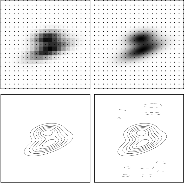
Figure 6: Upper panels: The images, in terms of brightness distributions, corresponding to the grid function $\{G_{j,k}\}$ given on $M=N=20$ square grid (on the left), and its reconstruction by 2-dimensional CEDCT series $F_{M,N}(x,y)$ (on the right). Lower panels: Contour plots of the analytic function $G(x,y)$ originating $\{G_{j,k}\}$ (on the left), and of its approximation by $F_{M,N}(x,y)$ (on the right). The original function $G(x,y)$ is composed of two-dimensional Gaussian distributions with transverse dispersions for both $\sigma_{\perp}=1/N=0.05$, an angle between long axes of the ellipsoids equal to $20^{\circ}$, and a small separation between their peak positions.

Example 6.  The latter case is chosen in Fig. 6 where the upper panels show, in terms of brightness distribution, the original grid function produced by 2 Gaussians with $\sigma_{1,\perp}=\sigma_{2,\perp}=0.05=1/N$, for $N=M=20$, and its reconstruction in the form of 2-dimensional continuous DGT extension (on the right). The major axes of the ellipsoids are inclined at a small angle ($20^{\circ}$) to each other. For comparison, on the bottom left panel we show the contour plot of the exact (i.e. originating) function $G(x,y)$, and the bottom right panel shows its approximation by 2-dimensional CEDGT. It is obvious that the reconstructed CEDGT image not only recovers the directions of the ellipsoids and their maxima, but it practically coincides with the exact image. Note that the dashed contours on both Fig. 5 and Fig. 6 show a level slightly below zero, $F_{MN}=-0.001$.

Generalization of the proposition for an n-dimensional DGT of a function $G(x_{1},\ldots,x_{n})$ on $[{\bf SU}(2)]^{n}$ group is straightforward:

Proposition: Let $G_{j_{1}\ldots j_{n}}=G(x_{1,j_{1}},\ldots,x_{n,j_{n}}$ be values of a bounded function $G(x^{(1)},\ldots,x^{(n)})$ given on the rectangular $(M_{1},\ldots,M_{n})$-interval grid points

$$\{x^{1,j_{1}}=j_{1}X_{1}/M_{1},\ldots,x^{n,j_{n}}=j_{n}X_{n}/M_{n}\,,\qquad j_{k}=0,1,\ldots,M_{k}\,:\;k=0,1,\ldots,n\}\;.$$

A continuous function given by finite Fourier series

$$F_{M_{1}\ldots M_{n}}(x_{1},\ldots,x_{n})=\sum_{m_{1}=0}^{M_{1}}\ldots\sum_{m_{n}=0}^{M_{n}}A_{m_{1}\ldots m_{n}}\cos\frac{\pi m_{1}x_{1}}{X_{1}}\cdot\ldots\cdot\cos\frac{\pi m_{n}x_{n}}{X_{n}}\;,$$ (48)

where

$$A_{m_{1}\ldots m_{n}} = \sum_{j_{1}=0}^{M_{1}}\ldots\sum_{j_{n}=0}^{M_{n}}\frac{C_{M_{1},m_{1}}C_{M_{1},j_{1}}\cdot\ldots\cdot C_{M_{n},m_{n}}C_{M_{n},j_{n}}}{2^{n}\,M_{1}\cdot\ldots\cdot M_{n}}\times$$ (49)

$$G_{j_{1}\ldots j_{n}}\,\cos\frac{\pi m_{1}j_{1}}{M_{1}}\cdot\ldots\cdot\cos\frac{\pi m_{n}j_{n}}{M_{n}}$$

satisfies the equality

$$F_{M_{1}\ldots M_{n}}(x_{j_{1}},\ldots,x_{j_{n}})=G_{j_{1}\ldots j_{n}}\;,\qquad{\rm for\;all}\;j_{k}\in\{0,1,\ldots,M_{k}\}\;{\rm and}\;k\in\{0,1,\ldots,n\}\;.$$

Furthermore, if $G(x_{1},\ldots,x_{n})$ is continuous, then $F_{M_{1}\ldots M_{n}}(x_{1},\ldots,x_{n})$ converges to $G(x_{1},\ldots x_{n})$ with $M_{1},\ldots,M_{n}\longrightarrow\infty$.

The proof of this proposition is readily obtained by the method of induction on the SU(2) factors of the group.

4.1 An example of CEDCT application to real images

In order to demonstrate the potential of the above suggested approach of continuous extension of the inverse multi-dimensional discrete group transforms for purposes of natural interpolation of discrete images between the grid points, as well as for the possibility of data compression and smooth representation of the compressed images, we have chosen a 56$\times$140 pixel fragment of the well known image “Lena”. The original fragment shown on Fig. 7a is strongly enlarged (‘zoomed’) in order to make visible the granularity of the image at its resolution limits. The grayscale color coding of the fragment contains all 256 intensity levels, from $g=0$ (black) to $g=255$ (white)

In Fig. 7b we show the continuous extension of the original image. It is constructed by subdividing each of the initial intervals $\Delta x$ and $\Delta y$ into 3 subintervals. This procedure increases the density of the grid points (pixels) by a factor $3\times 3=9$. Calculations are done dividing first the initial 56$\times$140 pixel fragment into ten 28$\times$28 pixel subfragments, then calculating the CEDCT for each of these sub-fragments. It allows us to demonstrate, on the next two panels, the effects of CEDCT image reconstruction at the block edges after some image compression is done. Because the continuous extension of the inverse DCT can formally extend the values of the initial intensity distribution function to values $F_{MN}(x,y)$ beyond the limits $[0,255]$ used for the intensity coding, we have linearly renormalized the values of $F_{NN}\rightarrow\tilde{F}_{NN}\in[0,255]$. The positive impact of the higher resolution achieved by the use of CEDCT in Fig. 7b, as compared with the original image in Fig. 7a, is apparent.

Note that the harmonic order of the cosine functions $\cos(\pi nx/X_{0}$ and $\cos(\pi my/Y_{0}$ used in CEDCT corresponds to the modes $0\leq m,n\leq 50$. In Fig. 7c we show the continuous extension of the image obtained after application of the simplest “low-pass compression” procedure (see e.g. [11]), putting the DCT coefficients $A_{mn}\rightarrow 0$ for all high-order modes with either $m$ or $n$ exceeding $n_{max}=19$. This procedure generally removes the high-frequency ‘noise’ from the image, and compresses the image by a factor $(29/20)^{2}\approx 2$. No visual degradation of the CEDCT image is apparent. It is noteworthy that although the exactness property of the transform in Fig. 7c is lost, the edges of the 10 individual blocks, or the sub-fragments, cannot be visually distinguished. The block edges become noticeable only in Fig. 7d, where we have applied again the CEDCT approach for visualization of the image compressed now by a factor of 10. The compression in Fig. 7d is effectively reached by keeping in CEDCT series only $10\%$ of the cosine terms with the large-value coefficients $A_{mn}$, and discarding all terms with small-value $A_{mn}$. For Fig. 7b it has corresponded to the assumption $A_{mn}\rightarrow 0$ if $\mid A_{mn}\mid\leq 0.05\,A_{\rm max}$, where $A_{\rm max}$ is the maximum absolute value of the coefficients $\{A_{mn}\mid\}$ (excluding $A_{00}$). Obviously, the image in Fig. 7d still remains smooth and quite recognizable.

We would like to note here that it has not been our aim in this paper to reach the goal of the best possible image compression. We believe, however, that through this paper our examples demonstrate the high potential of the developed approach of continuous extensions of DCT, and of the DGTs generally, as considered in the next Paper II for the SU(3) group, for purposes of practical applications, and in particular for image processing and compression.

5 Summary

We have shown that:

1.   A discrete Fourier transform of a grid function $\{g_{k}\mid k=0,1,\ldots,N\}$ on the orbit functions of Lie groups, abbreviated DGT, in the case of $SU(2)$ is reduced to the well known discrete cosine transform, namely to DCT-I, which is a known type of exact discrete transforms, like the standard DFT sequence.

2.   The principal difference between these 2 types of discrete Fourier transforms consists in the fact that DCT is based on the functions $\cos(k\pi t/T_{0})$ corresponding to $k\leq N$ trigonometric harmonics of both integer and half-integer orders, $n=k/2\leq N/2$, whereas the DFT utilizes trigonometric functions of integer $n$ only, but extending to orders $n\leq N$. This results in vital differences in the subsequent properties of DFT and DCT (or DGT generally).

3.   If the function $g(t)$ originating $\{g_{k}\}$ is a continuous function of $t\in[0,T_{0}]$, then the continuous extension of the (inverse) DCT sequence results in the function $f_{N}(t)$ which converges to the original $g(t)$ with increasing $N$ at all $t$. This property does not hold for the continuous extension of the standard DFT sequence, which shows profound oscillations between the points of the grid. Note that potentially this feature implies significantly smaller vulnerability of DCT to the truncation/approximation errors in the process of filtering as compared with the standard DFT. Therefore it could be the reason for the superior general performance of the DCT compared with the DFT (see [5]).

4.   Similar to canonical continuous Fourier transform polynomials with coefficients calculated by exact integrations, the CEDCT series satisfies the principle of locality. This property insures, in particular, that the computation errors connected, e.g., with noise or uncertainties in one segment of the data will not significantly affect the reconstructed CEDCT image on the distant segment of data. This property of DCT may become important especially in the process of lossy data compression when the property of exactness of the discrete transform is not necessarily preserved.

5.   Similar to the canonical CFT, the CEDCT series $f_{N}(t)$ can be differentiated term by term, so that for the (first) derivative series $\lim_{N\rightarrow\infty}f_{N}^{\prime}(t)\rightarrow g^{\prime}(t)$ for all $t\in(0,T_{0})$ provided that the second derivative of $g(t)$ is a continuous (or just an integrable) function on the interval $[0,T_{0}]$. For CEDCT this property is valid both when $g(0)=g(T_{0})$ and $g(0)\neq g(T_{0})$. It does not necessarily hold for other types of discrete Fourier transforms which might themselves be converging, like $s_{k}(t)$ in (27), but which produce nontheless a non-converging derivative series, as demonstrated in Fig. 4.

The derivative series $f_{N}^{\prime}(t)$ satisfies the localization principle along with $f_{N}(t)$.

6.   In the case of an $n$-dimensional function defined on the knots of a rectangular $n$-dimensional grid, the DGT Fourier decomposition can be performed using the orbit functions of $[SU(2)]^{n}$ group. Such Fourier series are effectively reduced to the $n$-fold convolution of one-dimensional DGT on SU(2) alongside $n$ independent (rectangular) axes, and therefore they posess nice properties of convergence, localization, and differentiability of their continuous DGT extensions similar to the one-dimensional CEDCT.

Figure 1: Approximation of an analytic function (20), shown by the dotted lines, with the CEDCT function $f_{N}(t)$ (solid lines) for the discrete interval numbers $N=10$ and $N=14$. The big dots show the values of the grid function $\{g_{k}\equiv g(t_{k})\}$ for $\{k=0,\ldots,N\}$. For comparison we also show by dashed lines the approximation of $g(t)$ by the exact CFT polynomials of (21) with $K=N/2$. It gives polynomials of the same harmonic maximum order as the ones in the DCT. The parameters in (20) are: $A1=2$, $A_{2}=1.5$, $\sigma_{1}=\sigma_{2}=0.05$, $t_{1}=0.42$, $t_{2}=0.56$.

Figure 2: Behaviours of the Fourier series $h_{N}(t)$ and $f_{N}(t)$, given by equations (25) and (15). Solid lines represent the CEDFT, and dashed lines show the CEDCT. Big dots show the values of the grid function $\{g_{k}\mid k=0,\ldots,N\}$ originated from an analytic function $g(t)$ which is given by equation (26), and is shown by the dot-dashed line.

Figure 3: Approximation of an analytic function $g(t)$ composed of two Gaussians, (20), with the CEDCT function $f_{N}(t)$ of (15) with $N=16$ (solid lines) and the Fourier series $s_{K}(t)$ of (27) that uses only the first $K\sim N/2$ coefficients $\{u_{j}\mid j\leq K\}$ of the standard DFT (23). The dashed line is for $K=N/2=8$, and the dot-dashed line corresponds to $K=6$. The full dots in the upper panel correspond to $\{g_{k}\mid k=0,\ldots,N\}$. The lower panel shows the corresponding errors of the approximation to $g(t)$ by these 3 types of discrete Fourier transforms. The dispersions in (20) are assumed to be $\sigma_{1}=0.07$ and $\sigma_{2}=0.2\,$.

Figure 4: The CEDCT series $f_{N}(t)$ (solid lines, top panels) and the derivatives $f_{N}^{\prime}(t)$ (solid lines, bottom panels) for an analytic function $g(t)$ of equation (40) and its derivative $g^{\prime}(t)$ (heavy dot-dashed lines) in the case of $N=14$ and $N=140$. For comparison, by dashed lines we show the truncated DFT series $s_{K}(t)$ of equation (27) and its derivative $s_{K}^{\prime}(t)$ with $K=N/2$. Note that although $s_{K}(t)$ converges with $N\rightarrow\infty$ at all $t\in(0,1)$, its derivative $s_{K}^{\prime}$ apparently does not.

Figure 5: Contour plots (upper panels) and visual ‘3D’ images (lower panels) of an analytic function $G(x,y)$ (right side) and its approximation by 2-dimensional $SU(2)$$\times$$SU(2)$ CEDGT/DCT series $F_{MN}(x,y)$ (left side) with $M=N=20$. $G(x,y)$ is composed of a sum of 2 two-dimensional Gaussian ellipsoids, each in the form of (47), and with dispersions $\sigma_{\perp,1}=\sigma_{\perp,2}=0.025=1/2N$. The dashed lines on the left bottom panel show the contour level $F_{MN}(x,y)=-0.001$ .

Figure 7: (a) Zoomed $56\times 140$-pixel fragment of the original image “Lena”; (b) CEDCT image calculated with the 3$\times$3 higher resolution, i.e. corresponding to $168\times 420$ pixels; For our calculations the image was first subdivided into 10 square blocks of $28\times 28$ size. (c) The picture in the same $168\times 420$ pixel representation compressed by a factor of 2. The compression is reached by retaining in (45) only the first $0\leq m,n\leq 19$ DCT coefficients $A_{mn}$, and discarding all higher-order terms. (d) The picture compressed by a factor of 10; the compression is achieved by discarding all cosine terms with $\mid A_{mn}\mid\leq 0.05\,A_{\rm max}$ (see text).

References

- [1] A. Zygmund, Trigonometric Series, Cambridge University Press (1959)
- [2] G. P. Tolstov, Fourier series, Dover, N-Y (1976)
- [3] R. V. Moody, J. Patera, Computation of character decompositions of class functions on compact semisimple Lie groups, Mathematics of Computation 48 (1987), 799-827
- [4] R. V. Moody, J. Patera Elements of finite order in Lie groups and their applications, XIII Int. Colloq. on Group Theoretical Methods in Physics, ed. W. Zachary, World Scientific Publishers, Singapore (1984), 308–318.
- [5] N. Ahmed, T. Natarajan, K. R. Rao, Discrete cosine transform, IEEE Trans. Comput. C-23 (1974), 90-93
- [6] Z. Wang, Fast algorithms for the discrete W transform and for the discrete Fourier transform, IEEE Trans. Acoust., Speech and Signal Process. ASSP-32 (1984), 803-816
- [7] G. Strang, The discrete cosine transform, SIAM Review 41 (1999), 135-147
- [8] E. O. Brigham, The fast Fourier transform, Prentice Hall, Englwood Cliffs, N.J. (1974)
- [9] A. V. Oppenheim, R. W. Schafer, Digital signal processing, Prentice-Hall, Englwood Cliffs (1975)
- [10] H. J. Nussbaumer, Fast Fourier transform and convolution algorithms, Springer-Verlag, Berlin Heidelberg N-Y (1982)
- [11] K. R. Rao, P. Yip, Discrete cosine transform - Algorithms, Advantages, Appliucations, Academic Press (1990)
- [12] V. G. Kac, Automorphisms of finite order of semisimple Lie Algebras, J. Funct. Anal. Appl. 3 (1969), 252-254
- [13] R. V. Moody, J. Patera, Characters of elements of finite order in simple Lie groups, SIAM J. on Algebraic and Discrete Methods 5 (1984), 359-383
- [14] W. G. McKay, R. V. Moody, J. Patera, Decomposition of tensor products of representations, Algebras, Groups and Geometries 3 (1986), 286-328
- [15] W. G. McKay, R. V. Moody, J. Patera, Tables of characters and decomposition of plethysms, in Lie algebras and related topics, Amer. Math. Society, Providence R.I., eds. D. J. Britten, F. W. Lemire, R. V. Moody (1985), 227–264
- [16] S. Grimm and J. Patera Decomposition of tensor products of the fundamental representations of , in Advances in Mathematical Sciences – CRM’s 25 Years, ed. L. Vinet, CRM Proc. Lecture Notes, Amer. Math. Soc., Providence, RI, 11 (1997) 329–355
- [17] R. N. Bracewell, Numerical transforms, Science (1990) 697–704
- [18] J. W. Cooley, and J. W. Tukey, An algorithm for the machine calculation of complex Fourier series, Mathematics of Computation 19 (1965), 297-301
- [19] W. M. Gentleman and G. Sande, Fast Fourier transform for fun and profit, AFIPS proc. 29 (1966), 563-578
- [20] R. C. Singleton, A method for Computing the fast Fourier transform with auxiliary memory and limited high-speed storage, IEEE Trans. Audio Electroacoust. AU-15 (1967), 91-97
- [21] C. M. Rader and N. M. Brenner, A new principle for fast Fourier transformation, IEEE Trans. ASSP-24 (1976)
- [22] S. Winograd, On computing the discrete Fourier transform, Mathematics of Computation 32 (1978), 175-199
- [23] M. J. Narasimha, A. M. Peterson, On the computation of the discrete cosine transform, IEEE Trans. Commun. COM-26 (1978), 934-946
- [24] B. D. Tseng, W. C. Miller, On computing the discrete cosine transform, IEEE Trans. Comput. C-27 (1978), 966-968
- [25] J. Makhoul, A fast cosine transform in one and two dimensions, IEEE Trans. Acoust. Speech, and Signal Process. ASSP-28 (1980), 27-34
- [26] M. Vetterli, H. Nussbaumer, Simple FFT and DCT algorithms with reduced number of operations, Signal Processing 6 (1984), 267-278