Exact Solutions for Loewner Evolutions

Abstract

In this note, we solve the Loewner equation in the upper half-plane with forcing function $\xi(t)$, for the cases in which $\xi(t)$ has a power-law dependence on time with powers $0$, $1/2$ and $1$. In the first case the trace of singularities is a line perpendicular to the real axis. In the second case the trace of singularities can do three things. If $\xi(t)=2\sqrt{\kappa t}$, the trace is a straight line set at an angle to the real axis. If $\xi(t)=2\sqrt{\kappa(1-t)}$, as pointed out by Marshall and Rohde [12], the behavior of the trace as $t$ approaches $1$ depends on the coefficient $\kappa$. Our calculations give an explicit solution in which for $\kappa<4$ the trace spirals into a point in the upper half-plane, while for $\kappa>4$ it intersects the real axis. We also show that for $\kappa=9/2$ the trace becomes a half-circle. The third case with forcing $\xi(t)=t$ gives a trace that moves outward to infinity, but stays within fixed distance from the real axis. We also solve explicitly a more general version of the evolution equation, in which $\xi(t)$ is a superposition of the values $\pm 1$.

Key words:

conformal map, Loewner equation, singularity, slit domain.

1 Introduction

The Loewner differential equation was introduced by Karl Löwner [11] (who later changed his name to Charles Loewner) to study properties of univalent functions on the unit disk. The differential equation is driven by a function that encodes in an ingeneous way continuous curves slitting the disk from the boundary. A few years ago, Oded Schramm realized that by taking Brownian motion as the driving function, the Loewner equation generates families of random curves with a conformally invariant measure, that he called “Stochastic Loewner Evolutions” (SLE’s) [13]. Moreover, he showed that if the loop-erased random walk has a scaling limit, and if this scaling limit is conformally invariant, then it must be described by an SLE, and he made similar conjectures about the scaling limits of uniform spanning trees and of critical percolation. The existence of conformally invariant scaling limits and the connections with SLE were established for the first two models by Lawler, Schramm and Werner [9], and for critical site percolation on the triangular lattice by Smirnov [14]. Over the past few years Schramm’s idea has been investigated further, mainly in a combined effort of Lawler, Schramm and Werner [5], leading to new developments in the study of (the scaling limit of) discrete models.

In SLE an ensemble of driving functions generates an ensemble of shapes. It is a difficult task to understand fully the relation between these two ensembles. For this reason we investigate here the simpler problem of the relation between a driving term in Loewner’s equation and the curve it generates, by explicit calculation. In particular we study exact, deterministic solutions of Loewner’s equation in the upper half $\mathcal{H}$ of the complex plane. One of the purposes of this study is to present some explicit examples that may help to elucidate the behavior of the curves generated by Loewner’s equation. For example, our solution for square-root forcing in section 4 shows a transition from a simple curve that stays above the real line to a curve intersecting the real line, which is similar to the transition occurring at $\kappa=4$ in SLE.

To get us started, we need to understand how the Loewner equation describes curves slitting the half-plane $\mathcal{H}$. So suppose that $\gamma(t)$, $t\geq 0$, is a simple curve in $\mathcal{H}$ emanating from the real line. Then according to conformal mapping theory, there exists a unique conformal mapping of the form $w=g_{t}(z)$ that takes the domain $\mathcal{R}$ consisting of all points in $\mathcal{H}$ minus those on the slit $\gamma[0,t]$ onto the upper half of the $w$-plane, in such a way that near infinity this map has the expansion

$$g_{t}(z)=z+c(t)/z+O(1/z^{2}).$$ (1)

See figure 1 for a schematic picture of the mapping. It is a theorem that the coefficient $c(t)$ (which is called the capacity) is continuously increasing with $t$. Therefore, the parameterization of the curve can be chosen such that $c(t)=2t$, and henceforth we assume that this is the case.

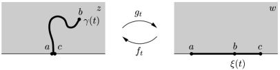
Figure 1: This figure shows how a slit $\gamma$ in the $z$-plane maps into a linear boundary in the $w$-plane. Notice that two neighbouring points in the $z$-plane have images which are far apart in the $w$-plane.

The conformal maps $g_{t}$ satisfy a surprisingly simple differential equation, which is the Loewner equation

$$\frac{dg_{t}}{dt}=\frac{2}{g_{t}-\xi(t)}$$ (2a)

with the initial condition

$$g_{0}=z$$ (2b)

for all $z$ in $\mathcal{H}$. Here, the value of $\xi$ at time $t$ is just the image of the point $\gamma(t)$ under the map $g_{t}$. We call $\xi(t)$ the driving function or forcing function of the Loewner equation. It is continuous and real-valued. (For a text-book discussion of Loewner’s equation and proofs of the above statements when the domain is the unit disk, see [2] and [4]. The half-plane case we are considering here is analogous and is discussed in [7] and [8]).

Conversely, the Loewner equation (2) has a solution for any given continuous real-valued function $\xi(t)$. This generates the function $g_{t}(z)$. For each value of $t$ this function can be thought of as a mapping of the form $w=g_{t}(z)$ which takes some connected subset of the upper-half $z$-plane, $\mathcal{R}$, into the entire region $\mathcal{H}$ above the real axis of the $w$-plane. Correspondingly, there exists an inverse function $f_{t}(w)$, which obeys $g_{t}(f_{t}(w))=w$ for all $w$ in the upper half-plane. This function maps the region $\mathcal{H}$ of the $w$-plane into the region $\mathcal{R}$ of the $z$-plane. It obeys the partial differential equation

$$\frac{\partial f_{t}(w)}{\partial t}=-\frac{2}{w-\xi(t)}\frac{\partial f_{t}(w)}{\partial w}.$$ (3)

The Loewner equation continually generates new singular points of $g_{t}$ that are mapped by $g_{t}$ onto the corresponding points $\xi(t)$ in the $w$-plane. Thus, as time goes on, points are continually removed from $\mathcal{R}$. If $\xi(t)$ is sufficiently smooth [12], these singular points form a simple curve $z_{c}(t)$, where the points $z_{c}(t)$ obey

$$g_{t}(z_{c}(t))=\xi(t).$$ (4)

This curve is called the trace of the Loewner evolution, but we also refer to it as the line of singularities. (Naturally, if we take $\xi(t)$ to be the driving function corresponding to a given curve $\gamma(t)$ as described above, then $z_{c}(t)$ will coincide with $\gamma(t)$).

Equations (2) have a simple scale invariance property under changing both the scale of space and of time. Any change of time of the form $t\mapsto\alpha^{2}t$ can be compensated by a change of scale. To do this, define a new $g$ and $\xi$ by

$$\tilde{g}_{t}(z):=\frac{1}{\alpha}g_{\alpha^{2}t}(\alpha z)\quad\mbox{and}\quad\tilde{\xi}(t)=\frac{1}{\alpha}\xi(\alpha^{2}t).$$ (5)

This pair then satisfies equations (2). Note that by the Schwarz reflection principle of complex analysis [1], the map $g_{t}$ extends to the lower half-plane and satisfies $g_{t}(\bar{z})=\overline{g_{t}(z)}$. It follows from equation (5) that flipping the sign of the forcing has the effect of reflecting the regions $\mathcal{R}$ and $\mathcal{H}$ (and hence also the line of singularities $z_{c}(t)$) in the imaginary axis. Likewise, a shift in the driving function $\xi(t)$ can be compensated by a similar shift in $g_{t}$, since the pair

$$\tilde{g}_{t}(z):=g_{t}(z-\alpha)+\alpha\quad\mbox{and}\quad\tilde{\xi}(t)=\xi(t)+\alpha$$ (6)

again solves equations (2). This shows that a shift in the driving function simply produces a shift of the same magnitude in the trace $z_{c}(t)$.

In this note we are interested in the question how the behavior of the trace is related to that of the driving function. This question can be investigated both numerically and, in some cases, by exact methods. A simple numerical method to find the trace generated by a given driving function $\xi(t)$, is to numerically integrate Loewner’s equation backwards from the initial condition $g_{t}=\xi(t)$ to obtain the value of $g_{0}=z_{c}(t)$. To deal with the singularity in Loewner’s equation, we can use the first-order approximation

$$g_{t}=g_{t-dt}+\frac{2\,dt}{g_{t-dt}-\xi(t-dt)}.$$ (7)

Substituting $g_{t}=\xi(t)$ and solving this equation for $g_{t-dt}$ gives an approximation for the value of $g$ at time $t-dt$, from where we then integrate backwards to obtain $g_{0}$. This method is good enough for the purpose of producing pictures. The figures 3, 4, 5 and 7 in this note were obtained in this way.

Exact solutions of equations (2) can be found in a few cases. The simplest are ones in which the forcing has one of the forms

$$\xi(t)=C(1-t)^{\beta}$$ (8a)

or

$$\xi(t)=Ct^{\beta}$$ (8b)

for $\beta=0$, $1/2$, and $1$. For a driving function of the form of equation (8b), a rescaling according to (5) gives the new forcing

$$\tilde{\xi}(t)=C\alpha^{2\beta-1}t^{\beta}.$$ (9)

This result allows us to scale away the constant $C$ when $\beta\neq 1/2$. For the special value $\beta=1/2$ the multiplicative constant can not be scaled away, and can be important in determining the form of the solution.

In sections 2, 3 and 4 we shall derive the solutions respectively for the powers $0$, $1$, and $1/2$. Section 5 contains an explicit construction of the maps $g_{t}$ for a half-plane slit by an arc, and we point out that this is a special case of square-root forcing with a finite-time singularity. In section 6 we consider a more general version of Loewner’s equation, where the forcing is a superposition of the values $\pm 1$ and produces two lines of singularities.

2 Constant Forcing

Here we look at the almost trivial situation in which $\beta=0$ and we can take

$$\xi(t)=A.$$ (10)

This situation is well-known (see for example [7] and appendix A in [3]), but for the sake of completeness we also treat it here. We could of course shift $A$ away by using equation (6), but this case is so easy that shifting is hardly worth the effort. The equation for $g$ can be solved by inspection, giving

$$g_{t}(z)=A+[(z-A)^{2}+4t]^{1/2}.$$ (11)

The inverse map is of the same form as the direct one, namely

$$f_{t}(w)=A+[(w-A)^{2}-4t]^{1/2}.$$ (12)

At time $t$, the function $g$ acquires a new singularity at the point

$$z_{c}(t)=A+2it^{1/2}$$ (13)

which maps under $g_{t}$ to the point $\xi(t)=A$ in the $w$-plane. Thus the singularities form a line segment parallel to the imaginary axis and the mapped region of the $z$-plane is the upper half-plane minus that line segment. The mapping has a singular point at the place where the trace meets the real axis. We can approach this point $z_{0}=A$ from two different directions, giving us two different images at the points

$$w_{0\pm}=A\pm 2t^{1/2}.$$ (14)

Figure 2 gives an illustration of the mapping.

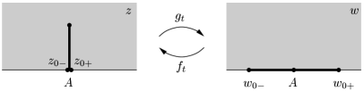
Figure 2: The trace produced by a constant forcing is a vertical line segment.

Because any smooth enough function $\xi(t)$ looks locally as if it were constant, we might expect that smooth $\xi(t)$’s generate traces of singularities which look like simple curves coming up from the real axis. In fact, one can prove that this statement is correct whenever $\xi(t)$ is sufficiently smooth so that it is Hölder continuous with exponent $1/2$ and sufficiently small norm, i.e. so that

$$\lim_{s\downarrow 0}\frac{|\xi(t-s)-\xi(t)|}{s^{1/2}}<C$$ (15)

for all $t$ and some constant $C$. The tricky issue is, when can it be that the curve will touch itself or hit the real line. Condition (15) is enough to ensure that this will not happen, as was shown by Marshall and Rohde [12], who did not give the value of the constant $C$. Our solution in section 4 below gives a specific example of the transition occuring at $C=4$. In a parallel and independent paper, Lind [10] proves also generally that Hölder-$1/2$ functions with coefficients $C<4$ generate slits.

3 Linear Forcing

The next case, not much harder, has the forcing increase linearly with time according to

$$\xi(t)=t.$$ (16)

We do not need an additive or multiplicative constant in equation (16) because these can be eliminated by equations (5) and (6). If we now redefine the independent variable to be $h=g-\xi$, then $h$ obeys

$$\frac{dh}{dt}=\frac{2-h}{h}=:-\frac{dh}{dF(h)}$$ (17)

where $F(h)$ is the function

$$F(h)=h+2\ln(2-h).$$ (18)

In terms of $F$ the solution is

$$F(h)=-t+c(z).$$ (19)

Here, $c(z)$ is a constant which must be set from the initial condition, $g_{0}=z$, giving the solution $F(h)=-t+F(z)$ or equivalently

$$F(g-t)=F(z)-t.$$ (20)

To find the trajectory of the singularity, use equations (4) and (20) to get

$$F(z_{c}(t))=F(0)+t=2\ln 2+t.$$ (21)

It is possible to find an explicit expression for this trajectory. To do so, substitute $2-z_{c}(t)=r_{t}\exp(-i\phi_{t})$ into the previous equation. Then split the equation in its real and imaginary parts to obtain

$$2\ln r_{t}-r_{t}\cos\phi_{t}=2\ln 2+t-2,$$ (22a)

$$r_{t}=2\phi_{t}/\sin\phi_{t}.$$ (22b)

After substituting the second equation into the first, it can be shown that $\phi$ increases monotonously in time from the value $\phi_{0}=0$ to $\phi_{\infty}=\pi$.

In terms of the parameter $\phi$, the line of singularities may be written explicitly as

$$z_{c}(t)=2-2\phi_{t}\cot\phi_{t}+2i\phi_{t}.$$ (23)

This shows that the line of singularities moves outward to infinity while remaining within a fixed distance of the real axis. Figure 3 shows the first part of this trajectory.

Figure 3: The shape of the line of singularities in the $z$-plane that arises from the forcing $\xi(t)=t$, up to time $t=100$.

For small and large values of $t$ we can also construct asymptotic forms of the solution (21). As $t$ goes to zero, one can expand $F(z_{c}(t))$ to third order in $z_{c}(t)$ and find that, to this order, the result is

$$z_{c}(t)=2it^{1/2}+\frac{2}{3}t+O(t^{3/2}).$$ (24)

For large $t$,

$$z_{c}(t)=t-2\ln[(t-2)/2]+2\pi i+O(\ln t/t).$$ (25)

4 Square-root Forcing

The next case, much more interesting, has the forcing be a square-root function of time. This case has two subcases: one in which the forcing has a finite-time singularity based on the rule of equation (8a), i.e.

$$\xi(t)=2[\kappa(1-t)]^{1/2},\qquad t\leq 1,\qquad\kappa\geq 0.$$ (26)

Here, as we shall see, the result changes qualitatively as $\kappa$ varies, with the critical case being $\kappa=4$ where the singular curve intersects the real axis. In the other situation, the forcing has an infinite-time singularity with the rule

$$\xi(t)=2[\kappa t]^{1/2},\qquad\kappa\geq 0.$$ (27)

In this case $z_{c}(t)$ is just a straight line, as is already clear from the scaling relation (5).

4.1 Infinite-time Singularity

To find the solution for the forcing (27), define the new variable $G=g/t^{1/2}$ and set $\tau=\ln t$. Then $G$ satisfies

$$\frac{dG}{d\tau}=-G/2+2/(G-2\kappa^{1/2})=\frac{(G-y_{+})(G-y_{-})}{2(2\kappa^{1/2}-G)}$$ (28)

where $y_{\pm}=\kappa^{1/2}\pm(\kappa+4)^{1/2}$. It follows that

$$\frac{dG}{d\tau}\left[\frac{y_{-}}{G-y_{+}}-\frac{y_{+}}{G-y_{-}}\right]=\frac{1}{2}(y_{+}-y_{-}).$$ (29)

Therefore, if we set

$$H(G):=\frac{2y_{+}\ln(G-y_{-})-2y_{-}\ln(G-y_{+})}{y_{+}-y_{-}}$$ (30)

then $dH(G)/d\tau=-1$ which integrates to

$$-H(G)=\tau+c(z)=\ln t+c(z).$$ (31)

The constant $c(z)$ can be determined from the observation that in the limit when $t$ approaches $0$,

$$H(G)+\ln t = \frac{2y_{+}\ln(g-{y_{-}}t^{1/2})-2y_{-}\ln(g-{y_{+}}t^{1/2})}{y_{+}-y_{-}}$$ (32)

$$\longrightarrow 2\ln z.$$

Our solution (31) for general $t$ becomes simply

$$H(g/t^{1/2})=2\ln(z/t^{1/2}).$$ (33)

Since the line of singularities is determined by the condition that $g$ is equal to the forcing we get

$$z_{c}(t)=B\,t^{1/2}\quad\mbox{where}\quad B=\exp[\frac{1}{2}H(2\kappa^{1/2})].$$ (34)

More explicitly the coefficient is

$$B=2\left(\frac{(\kappa+4)^{1/2}+\kappa^{1/2}}{(\kappa+4)^{1/2}-\kappa^{1/2}}\right)^{\displaystyle\frac{1}{2}\frac{\kappa^{1/2}}{(\kappa+4)^{1/2}}}\exp\left[\frac{1}{2}\pi i\left(1-\frac{\kappa^{1/2}}{(\kappa+4)^{1/2}}\right)\right],$$ (35)

so that the line of singularities is set at an angle to the real axis which is

$$\theta=\frac{1}{2}\pi\left(1-\frac{\kappa^{1/2}}{(\kappa+4)^{1/2}}\right).$$ (36)

For $\kappa=0$ the line is (as we know) perpendicular to the real axis while as $\kappa\rightarrow\infty$ the angle of intersection becomes smaller and smaller.

4.2 Finite-time Singularity

Now we turn to the forcing (26) with a singularity after a finite time. In this case, one can eliminate the time-dependence by using the new variable

$$G=g/(1-t)^{1/2}.$$ (37)

Then $G$ obeys

$$\frac{dG}{d\tau}=G/2+2/(G-2\kappa^{1/2})$$ (38)

where $\tau=-\ln(1-t)$. Once again the derivative becomes a simple function of the unknown, again appearing in the form of a ratio of polynomials, i.e.

$$-\frac{dG}{d\tau}=\frac{(G-y_{+})(G-y_{-})}{2(2\kappa^{1/2}-G)}.$$ (39)

where this time the roots are $y_{\pm}=\kappa^{1/2}\pm(\kappa-4)^{1/2}$. Notice that now the roots are real and positive when $\kappa\geq 4$ but that they are complex for $\kappa<4$. Thus we can expect a qualitative change in the solution at $\kappa=4$.

The integration of the equation proceeds exactly as in the previous case, giving the solution

$$H(G)=\tau+c(z)$$ (40)

where $H$ has the same form as before, but with different $y_{\pm}$:

$$H(G)=\frac{2y_{+}\ln(G-y_{-})-2y_{-}\ln(G-y_{+})}{y_{+}-y_{-}}.$$ (41)

The initial condition then implies that

$$H(g/(1-t)^{1/2})=-\ln(1-t)+H(z)$$ (42)

and the equation for the line of singularities is then

$$H(2\kappa^{1/2})=-\ln(1-t)+H(z_{c}(t)).$$ (43)

Note that equation (43) for the line of singularities tells us that $H(z_{c}(t))$ must approach $-\infty$ when $t$ approaches $1$. In the following subsections we shall consider the asymptotics of $z_{c}(t)$ in this limit in more detail. We separate the discussion into the two cases $\kappa<4$ and $\kappa>4$. Then the section is completed with the derivation of the shape of the critical line of singularities at $\kappa=4$.

4.2.1 The logarithmic Spiral for $\kappa<4$

When $\kappa<4$, the real and imaginary parts of $H(z)$ are

$$\mathop{\rm Re\,}\nolimits H(z) = \frac{\kappa^{1/2}}{(4-\kappa)^{1/2}}\mathop{\rm Arg\,}\nolimits(z-y_{-})+\ln|z-y_{-}|$$ (44a)

$$\hbox{}-\frac{\kappa^{1/2}}{(4-\kappa)^{1/2}}\mathop{\rm Arg\,}\nolimits(z-y_{+})+\ln|z-y_{+}|,$$

$$\mathop{\rm Im\,}\nolimits H(z) = \mathop{\rm Arg\,}\nolimits(z-y_{-})-\frac{\kappa^{1/2}}{(4-\kappa)^{1/2}}\ln|z-y_{-}|$$ (44b)

$$\hbox{}+\mathop{\rm Arg\,}\nolimits(z-y_{+})+\frac{\kappa^{1/2}}{(4-\kappa)^{1/2}}\ln|z-y_{+}|,$$

from which it follows easily that $H(2\kappa^{1/2})$ is a positive real constant. Since the real part of $H(z_{c}(t))$ must go to $-\infty$ when $t$ approaches $1$, we conclude that $z_{c}(1)=y_{+}$, since the other possible candidate for the limit, i.e. $y_{-}$, is in the wrong half-plane. It then follows from the observation that $\mathop{\rm Im\,}\nolimits H(z_{c}(t))$ must vanish, that the trace must have wrapped around $y_{+}$ an infinite number of times. Hence the line of singularities is spiralling in towards the point $y_{+}$, as is depicted in figure 4.

Figure 4: The trace of singularities for square-root forcing with different values of $\kappa<4$. Also shown is the limiting case $\kappa=4$ where the trace starts to hit the real line. All the curves have been translated to make them start in the origin at time $t=0$.

To find a more explicit expression for the asymptotics, notice that when $z_{c}(t)$ is close to $y_{+}$, we can make the approximations

$$\ln|z_{c}(t)-y_{-}|\approx\ln\left(2(4-\kappa)^{1/2}\right)\mbox{\ and\ }\mathop{\rm Arg\,}\nolimits(z_{c}(t)-y_{-})\approx\pi/2.$$ (45)

Splitting equation (43) in its real and imaginary parts, and substituting the above approximate values then gives a system of two equations that we can solve for the unknows $\ln|z_{c}(t)-y_{+}|$ and $\mathop{\rm Arg\,}\nolimits(z_{c}(t)-y_{+})$. This gives the result

$$\ln|z_{c}(t)-y_{+}| \approx \big{[}A(\kappa)+(4-\kappa)\ln(1-t)\big{]}/4,$$ (46a)

$$\mathop{\rm Arg\,}\nolimits(z_{c}(t)-y_{+}) \approx \big{[}B(\kappa)-\kappa^{1/2}(4-\kappa)^{1/2}\ln(1-t)\big{]}/4,$$ (46b)

where the constants are

$$A(\kappa) = \ln 16+(\kappa-2)\ln(4-\kappa)$$ (46c)

$$\hbox{}+(2\mathop{\rm Arg\,}\nolimits(y_{+})-\pi)\kappa^{1/2}(4-\kappa)^{1/2},$$

$$B(\kappa) = \kappa^{1/2}(4-\kappa)^{1/2}\ln(4-\kappa)$$ (46d)

$$\hbox{}+(\pi-2\mathop{\rm Arg\,}\nolimits(y_{+}))\kappa-2\pi.$$

Thus, the distance between $z_{c}(t)$ and $y_{+}$ is decreasing like a power law in $t$, whereas the winding number of $z_{c}(t)$ around $y_{+}$ grows only logarithmically.

4.2.2 The Intersection for $\kappa>4$

Figure 5: For a square-root forcing with $\kappa\geq 4$ the line of singularities intersects the real line at an angle that varies with $\kappa$. The curves were translated to make them start in the origin.

For $\kappa>4$ the real and imaginary parts of $H(z)$ are

$$\mathop{\rm Re\,}\nolimits H(z) = \left(1+\frac{\kappa^{1/2}}{(\kappa-4)^{1/2}}\right)\ln|z-y_{-}|$$ (47a)

$$\hbox{}+\left(1-\frac{\kappa^{1/2}}{(\kappa-4)^{1/2}}\right)\ln|z-y_{+}|,$$

$$\mathop{\rm Im\,}\nolimits H(z) = \left(1+\frac{\kappa^{1/2}}{(\kappa-4)^{1/2}}\right)\mathop{\rm Arg\,}\nolimits(z-y_{-})$$ (47b)

$$\hbox{}+\left(1-\frac{\kappa^{1/2}}{(\kappa-4)^{1/2}}\right)\mathop{\rm Arg\,}\nolimits(z-y_{+}),$$

and $H(2\kappa^{1/2})$ is again a positive real number. This time, as $t$ approaches one, $z_{c}(t)$ must approach the point $y_{-}$ on the real line, see figure 5. In fact, we can calculate the angle at which the line of singularities intersects the real line from the observation that $\mathop{\rm Im\,}\nolimits H(z_{c}(t))$ must vanish.

Indeed, if we denote by $\phi$ the angle at which $z_{c}(t)$ hits the real line (measured from the real line in the positive direction), then we have that in the limit $t\rightarrow 1$, $\mathop{\rm Arg\,}\nolimits(z_{c}(t)-y_{+})\rightarrow\pi$ whereas $\mathop{\rm Arg\,}\nolimits(z_{c}(t)-y_{-})\rightarrow\phi$. The condition $\mathop{\rm Im\,}\nolimits H(z_{c}(t))=0$ then gives

$$\phi=\pi\frac{\kappa^{1/2}-(\kappa-4)^{1/2}}{\kappa^{1/2}+(\kappa-4)^{1/2}}$$ (48)

when $t$ goes to $1$. As we can see, we have a glancing incidence for $\kappa=4$ and $\kappa\rightarrow\infty$, while for $\kappa=9/2$ the incidence is perpendicular. In fact we can prove that for $\kappa=9/2$ the line of singularities is a half-circle of radius $\sqrt{2}$. We will do this in section 5, where we give an explicit construction of the conformal maps $g_{t}$ when the half-plane is slit by a half-circle.

4.2.3 The critical Curve at $\kappa=4$

It is not difficult to find an explicit expression for the critical line of singularities at $\kappa=4$. In this case, the two roots in equation (39) are the same, $y_{\pm}=2$, and the equation can be rewritten as

$$\left[\frac{2}{G-2}-\frac{4}{(G-2)^{2}}\right]\frac{dG}{d\tau}=1.$$ (49)

Integration is straightforward and gives

$$2\ln(G-2)+\frac{4}{G-2}=-\ln(1-t)+2\ln(z-2)+\frac{4}{z-2}$$ (50)

where we have determined the integration constant from the initial condition $G_{0}=g_{0}=z$. The line of singularities is determined by the condition that for $z=z_{c}(t)$, $G=4$.

Substituting $z_{c}(t)-2=r_{t}\exp(i\phi_{t})$ and splitting the equation in real and imaginary parts leads to the expression

$$z_{c}(t)=2+\frac{\sin 2\phi_{t}}{\phi_{t}}+2i\frac{\sin^{2}\phi_{t}}{\phi_{t}}$$ (51)

for the critical curve in terms of the parameter $\phi$. This parameter $\phi$ increases monotonously with time from $\phi_{0}=0$ to $\phi_{1}=\pi$.

5 Loewner Evolution for a growing Arc

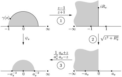
Figure 6: The construction of the map $\psi_{s}$ taking $\mathcal{H}$ minus the slit $\gamma[0,s]$ onto $\mathcal{H}$, in three steps. The illustration also tracks the images of the upper half of the unit disk and of the four “special” points $-1$, $0$, $\gamma(s)$ and $\infty$. The definitions of $\gamma(s)$, $R_{s}$ and $a_{s}$ are in the text.

In this section, we consider the situation where the upper half-plane $\mathcal{H}$ is slit by the curve $\gamma(s)=\exp(is)$, $s\in\left[0,\pi\right)$. The idea is to construct the conformal maps that map the half-plane minus the slit $\gamma[0,s]$ back to the half-plane and have the expansion of equation (1). After reparameterizing time one can then identify the driving function, and verify that the obtained maps $g_{t}$ satisfy Loewner’s equation. The form of the normalized maps and of the driving function already appears in appendix A of [3], but for completeness we present a short account of the derivation of these results below. A simple rescaling argument then allows us to make the connection with section 4 and prove that the square-root forcing we considered there generates a half-circle of radius $\sqrt{2}$ when $\kappa=9/2$.

To obtain the normalized conformal maps, we start by constructing the map $\psi_{s}$ of figure 6 as the composition of the three maps depicted there. The explicit form of this map is

$$\psi_{s}(z)=\frac{1}{a_{s}^{2}}\frac{a_{s}+f_{s}(z)}{a_{s}-f_{s}(z)}\qquad\mbox{for\ }z\in\mathcal{H}\setminus\gamma[0,s]$$ (52)

where $a_{s}:=\cos(s/2)^{-1}$ and the function $f_{s}(z)$ is given by

$$f_{s}(z)=\sqrt{\Big{(}\frac{z-1}{z+1}\Big{)}^{2}+R_{s}^{2}}=\sqrt{a_{s}^{2}-\frac{4z}{\smash{(z+1)^{2}}}},$$ (53)

with $R_{s}:=\tan(s/2)$. We can now expand $\psi_{s}$ for large $z$, and identify the capacity $c(s)$. A simple translation will then give us the map satisfying (1).

Expanding $\psi_{s}(z)$ for large $z$ up to order $1/z$ gives

$$\psi_{s}(z)=z+(2-2a_{s}^{-2})+(1-a_{s}^{-4})/z+O(1/z^{2}).$$ (54)

Therefore, the map $\psi_{s}+2a_{s}^{-2}-2$ has the expansion of equation (1), with capacity $c(s)=1-a_{s}^{-4}$. The proper time reparameterization that makes the capacity equal to $2t$ is given by

$$2t(s):=1-a_{s}^{-4}=1-\cos^{4}(s/2)\quad\mbox{for}\quad s\in\left[0,\pi\right)$$ (55)

which has the inverse

$$s(t)/2=\arccos\left((1-2t)^{1/4}\right)\quad\mbox{for}\quad t\in\left[0,1/2\right).$$ (56)

The maps $g_{t}$ are then given by $g_{t}(z)=\psi_{s(t)}(z)+2a_{s(t)}^{-2}-2$. More explicitly, this can be written in the form

$$g_{t}(z)=\frac{2(z-1)^{2}+4z(1-2t)^{1/2}+2(z+1)\sqrt{(z+1)^{2}-4z(1-2t)^{1/2}}}{4z}.$$ (57)

We know from figure 6 that this map takes the point $\gamma(s(t))$ onto the image $3a_{s(t)}^{-2}-2$, which implies that the driving function must be

$$\xi(t)=3(1-2t)^{1/2}-2.$$ (58)

Indeed, one can check by differentiating (57) with respect to time, that $g_{t}$ satisfies Loewner’s equation with this driving function.

To make the connection with section 4, we note that a rescaling of the form (5) with $\alpha=1/\sqrt{2}$ turns the driving function into a function of the form of equation (26) with $\kappa=9/2$, up to a translation. We conclude that this particular square-root forcing produces a line of singularities that is a half-circle of radius $\sqrt{2}$.

We conclude this section with a discussion of its relation to an old paper by Kufarev [6]. Kufarev considers the equivalent of Loewner’s equation (2) in the unit disk, and gives an explicit solution of this equation for negative times. A half-plane version of Kufarev’s example is obtained as follows. Suppose that we set $\xi(-s)=3\sqrt{2s}$ for $s\geq 0$. Then it can be verified that the solution of (2) at time $-s$ is the normalized map that takes $\mathcal{H}$ onto $\mathcal{H}$ minus the half-disk of radius $\sqrt{2s}$ centered at $2\sqrt{2s}$. Observe that for $s=1/2$, up to a translation, this solution is just the inverse of (57) at time $t=1/2$. This is not a coincidence because generally, if one sets $\xi(-t):=\xi(T-t)$ and solves Loewner’s equation for both $g_{T}$ and $g_{-T}$, the two results are related by $g_{-T}=g_{T}^{-1}$.

6 Multivalued Forcing

In this section we look at a special case of the more general version of Loewner’s equation (appearing for example in [7])

$$\frac{dg_{t}}{dt}=\int\frac{2}{g_{t}-x}\,d\mu_{t}(x)$$ (59)

where $\mu_{t}$ is a measure on the real line that can be time-dependent. Here we will take $\mu_{t}$ to be time-independent and assigning a mass $p_{j}$ to the values $\xi_{j}$ such that $\sum_{j}p_{j}=1$. Then the equation for $g$ takes the form

$$\frac{dg}{dt}=\sum_{j}\frac{2p_{j}}{g-\xi_{j}}.$$ (60)

This can be seen as a case where the forcing $\xi(t)$ is a superposition of values, and we also believe that this can be described as a case where the forcing $\xi(t)$ makes rapid (random) jumps between the values $\xi_{j}$.

Equations like (60) are generally easily integrated. Take the specific case in which the possible values of $\xi$ are $\pm 1$, which are taken on with equal probability. Then equation (60) becomes

$$\frac{dg}{dt}=\frac{2g}{g^{2}-1}$$ (61)

which then integrates to give

$$g^{2}/2-\ln g=2t+z^{2}/2-\ln z.$$ (62)

There are two traces, starting respectively from $z=\pm 1$ and then moving upward towards $i\infty$. The traces are found, as before, by setting $g$ equal to the forcing. Thus the right-hand trace obeys

$$z_{c+}(t)^{2}-2\ln z_{c+}(t)=1-4t.$$ (63)

Figure 7: A forcing that is a superposition of the values $\pm 1$ produces two lines of singularities that approach each other as time goes on. This illustration shows the two lines up to time $t=10$.

Again we can obtain an explicit expression for the trace, like we did for the case of linear forcing in section 3, and for the critical curve in section 4. After substituting $z_{c}(t)=r_{t}\exp(i\phi_{t})$ and splitting the previous equation in real and imaginary parts, we obtain

$$z_{c\pm}(t)=\sqrt{\frac{2\phi_{t}}{\sin(2\phi_{t})}}\,\Big{(}\pm\cos\phi_{t}+i\sin\phi_{t}\Big{)}$$ (64)

where $\phi$ increases with time from the value $\phi_{0}=0$ to $\phi_{\infty}=\pi/2$. Note that we have filled in the results for both traces, using the fact that they must be symmetrically placed about the imaginary axis. We can also compute the asymptotics. For small values of $t$ we obtain

$$z_{c\pm}(t)=\pm 1+i\sqrt{2t}\mp\frac{1}{3}t+O(t^{3/2})$$ (65)

while for large values of $t$ the traces behave like

$$z_{c\pm}(t)=i\sqrt{(4t-1)-\ln(4t-1)}\pm\frac{\pi}{2(4t-1)^{1/2}}+O(\ln t/t^{3/2}).$$ (66)

We see that as the traces move upward, they also approach one another, as is shown in figure 7.

Acknowledgements

One of us (LPK) would like to thank Leiden University and Professor Wim van Saarloos for their hospitality for a part of the period in which the work was performed. We have had useful conversations about this research with Paul Wiegmann, Ilya Gruzberg, Isabelle Claus, Marko Kleine Berkenbusch, and John Cardy. We thank Steffen Rohde and Joan Lind for sharing their recent work on Loewner’s equation with us. LPK would like to acknowledge partial support from the US NSF’s Division of Materials Research. WK is supported by the Stichting FOM (Fundamenteel Onderzoek der Materie) in the Netherlands.

References

- [1] L. V. Ahlfors, Complex analysis: an introduction to the theory of analytic functions of one complex variable. McGraw-Hill, New York, second edition (1966).
- [2] L. V. Ahlfors, Conformal invariants: topics in geometric function theory. McGraw-Hill, New York (1973).
- [3] M. Bauer, D. Bernard, Conformal field theories of Stochastic Loewner Evolutions. Commun. Math. Phys. 239, pp. 493-521 (2003); arXiv: hep-th/0210015.
- [4] P. L. Duren, Univalent functions. Springer-Verlag, New York, 1983.
- [5] An overview of the literature on Schramm’s Loewner Evolutions (SLE) is given in Ilya A. Gruzberg and Leo P. Kadanoff, The Loewner equation: maps and shapes; arXiv: cond-mat/0309292.
- [6] P. P. Kufarev, A remark on integrals of Loewner’s equation, Doklady Akad. Nauk SSSR 57, pp. 655–656 (1947), in Russian.
-
[7]
G. F. Lawler, An introduction to the Stochastic Loewner
Evolution, available online at URL
http://www.math.duke.edu/jose/papers.html - [8] G. F. Lawler, O. Schramm, W. Werner, Values of Brownian intersection exponents I: Half-plane exponents. Acta Math. 187, 2, pp. 237–273 (2001); arXiv: math.PR/9911084.
- [9] G. F. Lawler, O. Schramm, W. Werner, Conformal invariance of planar loop-erased random walks and uniform spanning trees. Ann. Probab. (to appear); arXiv: math.PR/0112234.
- [10] J. R. Lind, A sharp condition for the Loewner Equation to generate slits; arXiv: math.CV/0311234.
- [11] K. Löwner, Untersuchungen über schlichte konforme Abbildungen des Einheitskreises, I. Math. Ann. 89, pp. 103–121 (1923).
-
[12]
D. E. Marshall and S. Rohde, The Loewner differential
equation and slit mappings, available online at URL
http://www.math.washington.edu/rohde/ - [13] O. Schramm, Scaling limits of loop-erased random walks and uniform spanning trees. Israel J. Math. 118, pp. 221–288 (2000); arXiv: math.PR/9904022.
- [14] S. Smirnov, Critical percolation in the plane: conformal invariance, Cardy’s formula, scaling limits. C. R. Acad. Sci. Paris Sér. I. Math. 333, 3, pp. 239–244 (2001). A longer version is available online at URL http://www.math.kth.se/stas/papers/