to appear in Celestial Mechanics
Non-integrability of the problem of a rigid satellite in gravitational and magnetic fields

Abstract

In this paper we analyse the integrability of a dynamical system describing the rotational motion of a rigid satellite under the influence of gravitational and magnetic fields. In our investigations we apply an extension of the Ziglin theory developed by Morales-Ruiz and Ramis. We prove that for a symmetric satellite the system does not admit an additional real meromorphic first integral except for one case when the value of the induced magnetic moment along the symmetry axis is related to the principal moments of inertia in a special way.

1 Introduction

Let us consider a rigid body $\mathcal{B}$ with mass $m$ and centre of mass $O_{1}$ moving in the gravitational field of a point $O$ with mass $M$, see Fig.1. We assume that the orbit is circular and that it lies in the $(x,y)$-plane in the inertial reference frame defined by the orthonormal versors $\{\boldsymbol{e}_{1},\boldsymbol{e}_{2},\boldsymbol{e}_{3}\}$ with the origin at $O$. The principal axes reference frame of the body with the origin at $O_{1}$ is given by the orthonormal versors $\{\boldsymbol{a}_{1},\boldsymbol{a}_{2},\boldsymbol{a}_{3}\}$. We describe the rotational motion of the body with respect to the orbital reference frame $\{\boldsymbol{s},\boldsymbol{t},\boldsymbol{n}\}$ with the origin at $O_{1}$. Its axes lie along the radius vector of the centre of mass of the body, the tangent to the orbit in the orbital plane, and the normal to the orbital plane, respectively.

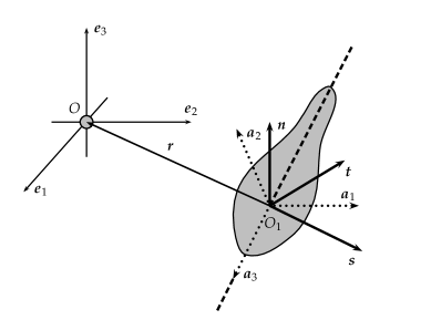
Figure 1: A rigid satellite in an orbit around a gravitational centre

We accept the following convention, see Arnold:78:: . For a vector $\boldsymbol{q}$ we denote by ${\mathbf{Q}}=[Q_{1},Q_{2},Q_{3}]^{T}$ the associate coordinates in the body frame, i.e., $Q_{i}=\boldsymbol{a}_{i}\cdot\boldsymbol{q}$, for $i=1,2,3$. For two vectors $\boldsymbol{q}$ and $\boldsymbol{p}$ we denote their scalar and vector products by $\boldsymbol{q}\cdot\boldsymbol{p}$ and $\boldsymbol{q}\times\boldsymbol{p}$, expressed in terms of their coordinates in the body frame by $\langle{\mathbf{Q}},{\mathbf{P}}\rangle$, and $[{\mathbf{Q}},{\mathbf{P}}]$, respectively. Thus we have

$$\langle{\mathbf{Q}},{\mathbf{P}}\rangle:=\sum_{i=1}^{3}Q_{i}P_{i}={\mathbf{Q}}^{T}{\mathbf{P}}=\boldsymbol{q}\cdot\boldsymbol{p},$$

and

$$[{\mathbf{Q}},{\mathbf{P}}]:=\begin{bmatrix}Q_{2}P_{3}-Q_{3}P_{2}\\ Q_{3}P_{1}-Q_{1}P_{3}\\ Q_{1}P_{2}-Q_{2}P_{1}\end{bmatrix}=\begin{bmatrix}(\boldsymbol{q}\times\boldsymbol{p})\cdot\boldsymbol{a}_{1}\\ (\boldsymbol{q}\times\boldsymbol{p})\cdot\boldsymbol{a}_{2}\\ (\boldsymbol{q}\times\boldsymbol{p})\cdot\boldsymbol{a}_{3}\end{bmatrix}.$$

The equations of the rotational motion of the body can be written in the following form

$$\begin{split}\frac{\mathrm{d}\phantom{t}}{\mathrm{d}t}{\mathbf{M}}&=[{\mathbf{M}},\boldsymbol{\Omega}]+{\mathbf{P}},\\ \frac{\mathrm{d}\phantom{t}}{\mathrm{d}t}{\mathbf{N}}&=[{\mathbf{N}},\boldsymbol{\Omega}],\\ \frac{\mathrm{d}\phantom{t}}{\mathrm{d}t}{\mathbf{S}}&=[{\mathbf{S}},\boldsymbol{\Omega}-\omega_{\mathrm{O}}{\mathbf{N}}],\end{split}$$ (1)

where ${\mathbf{M}}$, $\boldsymbol{\Omega}:={\mathbf{I}}^{-1}{\mathbf{M}}$, ${\mathbf{I}}:=\operatorname{diag}(A,B,C)$ are the angular momentum, the angular velocity and the inertia tensor of the body, respectively; $\omega_{\mathrm{O}}$ denotes the orbital angular velocity of the centre of mass of the body and ${\mathbf{P}}$ is the torque acting on the body. The explicit form of ${\mathbf{P}}$ depends on a particular model. The gravity-gradient torque is usually approximated by the following formula

$${\mathbf{P}}_{\mathrm{G}}:=3\omega_{\mathrm{K}}^{2}[{\mathbf{S}},{\mathbf{I}}{\mathbf{S}}],$$

where

$$\omega_{\mathrm{K}}^{2}=\frac{GM}{r^{3}},$$

and $r$ is the radius of the orbit, see Beletskii:65:: ; Beletskii:75:: ; Duboshin:68:: . Let us note that in the case of a circular Keplerian orbit $\omega_{\mathrm{O}}=\omega_{\mathrm{K}}$. Examples of models with $\omega_{\mathrm{O}}\neq\omega_{\mathrm{K}}$ can be found in Maciejewski:97::c ; Maciejewski:01::j .

In this paper we consider the case when, in addition to the gravitational torque, also the magnetic torque plays a significant role. Namely, we assume that the gravity centre (the Earth) is the source of a magnetic field which can be well approximated by a magnetic dipole whose axis coincides with $\boldsymbol{e}_{3}$. Modelling of the magnetic torque ${\mathbf{P}}_{\mathrm{M}}$ is generally difficult because it depends not only on the presence of constant magnets located in the satellite, but also on magnetic and conductive properties of the material used for its construction, as well as on the presence of electronic equipment, for details see Beletskii:85:: . In this paper we assume that the magnetic moment of the satellite is induced by the magnetic field of the central body, and, moreover, that the body is magnetically symmetric along an axis $\boldsymbol{l}$ fixed in the body. Then we have

$${\mathbf{P}}_{\mathrm{M}}:=\xi\langle{\mathbf{L}},{\mathbf{N}}\rangle[{\mathbf{L}},{\mathbf{N}}],$$

where $\xi$ is a parameter depending on the strength of the central magnetic dipole and magnetic properties of the body.

Thus, we consider the following system

$$\left.\begin{split}\frac{\mathrm{d}\phantom{t}}{\mathrm{d}t}{\mathbf{M}}&=[{\mathbf{M}},\boldsymbol{\Omega}]+3\omega_{\mathrm{K}}^{2}[{\mathbf{S}},{\mathbf{I}}{\mathbf{S}}]+\xi\langle{\mathbf{L}},{\mathbf{N}}\rangle[{\mathbf{L}},{\mathbf{N}}],\\ \frac{\mathrm{d}\phantom{t}}{\mathrm{d}t}{\mathbf{N}}&=[{\mathbf{N}},\boldsymbol{\Omega}],\\ \frac{\mathrm{d}\phantom{t}}{\mathrm{d}t}{\mathbf{S}}&=[{\mathbf{S}},\boldsymbol{\Omega}-\omega_{\mathrm{O}}{\mathbf{N}}].\end{split}\qquad\right\}$$ (2)

It possesses the Jacobi type first integral

$$H=\frac{1}{2}\langle{\mathbf{M}},{\mathbf{I}}^{-1}{\mathbf{M}}\rangle-\omega_{\mathrm{O}}\langle{\mathbf{M}},{\mathbf{N}}\rangle+\frac{3}{2}\omega_{\mathrm{K}}^{2}\langle{\mathbf{S}},{\mathbf{I}}{\mathbf{S}}\rangle-\frac{1}{2}\xi\langle{\mathbf{L}},{\mathbf{N}}\rangle^{2},$$ (3)

and three geometric first integrals

$$H_{2}=\langle{\mathbf{S}},{\mathbf{S}}\rangle,\qquad H_{3}=\langle{\mathbf{N}},{\mathbf{N}}\rangle,\qquad H_{4}=\langle{\mathbf{N}},{\mathbf{S}}\rangle.$$ (4)

The above equations can be rewritten in the Hamiltonian form

$$\frac{\mathrm{d}\phantom{t}}{\mathrm{d}t}M_{i}=\{M_{i},H\},\qquad\frac{\mathrm{d}\phantom{t}}{\mathrm{d}t}N_{i}=\{N_{i},H\},\qquad\frac{\mathrm{d}\phantom{t}}{\mathrm{d}t}S_{i}=\{S_{i},H\},\qquad i=1,2,3,$$ (5)

where the Poisson bracket $\{\cdot,\cdot\}$ is defined by

$$\begin{split}\{M_{i},M_{j}\}&=-\sum_{k=1}^{3}\varepsilon_{ijk}M_{k},\qquad\{M_{i},N_{j}\}=-\sum_{k=1}^{3}\varepsilon_{ijk}N_{k},\\ \{M_{i},S_{j}\}&=-\sum_{k=1}^{3}\varepsilon_{ijk}S_{k},\qquad\{N_{i},N_{j}\}=\{S_{i},S_{j}\}=\{N_{i},S_{j}\}=0,\end{split}$$ (6)

where $\varepsilon_{ijk}$ is the Levi-Civita symbol. This Poisson bracket is degenerated and the three geometric integrals (4) are its Casimirs. Their common levels are symplectic manifolds Marsden:99:: . From the geometric interpretation of the vectors ${\mathbf{N}}$ and ${\mathbf{S}}$ it follows that, for further study, we can select the following six dimensional symplectic leaf

$${\mathcal{M}}^{6}=\{({\mathbf{M}},{\mathbf{N}},{\mathbf{S}})\in\mathbb{R}^{9}\,|\,\,\langle{\mathbf{S}},{\mathbf{S}}\rangle=1,\quad\langle{\mathbf{N}},{\mathbf{N}}\rangle=1,\quad\langle{\mathbf{N}},{\mathbf{S}}\rangle=0\},$$ (7)

which is diffeomorphic to $\mathbb{R}^{3}\times\mathrm{SO}(3,\mathbb{R})$.

Remark 1.

The configuration space of a rigid body whose centre of mass moves in a prescribed orbit is $\mathrm{SO}(3,\mathbb{R})$ — all possible orientations of the body with respect to the orbital frame. Thus the classical phase space of the system is $T^{*}\mathrm{SO}(3,\mathbb{R})\simeq\mathbb{R}^{3}\times\mathrm{SO}(3,\mathbb{R})$.

Remark 2.

We can look at system (2) as a Hamiltonian system defined on a nine dimensional Poisson manifold which is ${\mathfrak{s}}^{*}$ — the dual to nine dimensional Lie algebra ${\mathfrak{s}}=(\mathbb{R}^{3}\times\mathbb{R}^{3})\rtimes\mathrm{so}(3,\mathbb{R})$ (here $\rtimes$ denotes the semi-direct product of Lie algebras). Then the Poisson bracket defined by (6) is the standard Berezin-Kostant-Kirillov-Souriou bracket, and ${\mathcal{M}}^{6}$ is a co-adjoint orbit, see Marsden:99:: . Here we refer the reader to paper Audin:02:: where the case of a rigid satellite without the influence of magnetic torques is considered.

System (2) depends on the parameters $p:=(A,B,C,\omega_{\mathrm{O}},\omega_{\mathrm{K}},L_{1},L_{2},L_{3},\xi)$. They belong to a set

$${\mathcal{P}}:=\{p\in\mathbb{R}_{+}^{5}\times\mathbb{R}^{4}\;|\;\langle{\mathbf{L}},{\mathbf{L}}\rangle=1,\quad A<B+C,\quad B<C+A,\quad C<A+B,\},$$

whose interior is an eight-dimensional subset of $\mathbb{R}_{+}^{5}\times\mathbb{R}^{4}$ ($\mathbb{R}_{+}$ denotes the positive real axis).

It is natural to ask for which $p\in{\mathcal{P}}$ system (2) or its restriction to ${\mathcal{M}}^{6}$ admits one or two additional first integrals. The high dimensionality of the system and a big number of parameters make this problem very difficult. Let us enumerate some known facts.

1. For $\xi=0$ (the magnetic torque vanishes) the only known completely integrable case is a spherically symmetric case $A=B=C$. This case is trivial because for a spherically symmetric body the gravitational torque vanishes. There is no proof that system (2) is non-integrable when $\xi=0$ and the body is not spherically symmetric.

2. For $\xi=0$ and an axially symmetric body, e.g. $A=B$, system (2) admits one additional first integral, namely $H_{5}=M_{3}$. There is no proof that this is the only situation when system (2) possesses one additional first integral.

3. For $A=B=C$ only the magnetic torque acts on the body. System (2) is completely integrable and the additional first integrals are $H_{5}=\langle{\mathbf{M}},{\mathbf{N}}\rangle$ and $H_{6}=\langle{\mathbf{M}},{\mathbf{L}}\rangle$. In this case the first two equations form a closed subsystem which coincides with a special case of the Kirchhoff equations for a rigid body in ideal fluid in the integrable case of Clebsh, see Kozlov:96:: .

Some limiting cases of system (2) when $\omega_{\mathrm{O}}=0$, or $\omega_{\mathrm{K}}=0$ are worth mentioning because they are related to very well known systems.

Let us consider the case $\omega_{\mathrm{O}}=0$. Now, system (2) describes the rotational motion of a rigid body with the mass centre fixed in the external gravity and magnetic fields. For $\xi=0$ the first and the third equation in (2) form a closed subsystem which coincides with the equations of motion of the completely integrable Brun problem Brun:1893:: , see also Bogoyavlenskii:85::a . When $\omega_{\mathrm{K}}=0$, a subsystem of (2) consisting of the first two equations, is again a special case of the Kirchhoff equations, see Kozlov:96:: .

The aim of this paper is to study the integrability of system (2) when the body is axially symmetric. For this purpose we apply the Morales-Ramis theory Morales:99:: ; Morales:01::b which is an extension of the Ziglin theory Ziglin:82::b ; Ziglin:83::b . Both theories are based on a study of variational equations around a particular non-equilibrium solution of the complexified system. We can associate with the variational equations the monodromy and the differential Galois groups. When the system is integrable, then these groups are of a special form and this fact gives a necessary condition for integrability. To make the paper self-contained, we present basic theoretical facts concerning the Ziglin and Morales-Ramis theory in the next section. More technical material needed in our investigation is presented in the Appendix. We present both theories trying to avoid formal language, and we give several examples, which, as we hope, helps to understand basic notions of both theories and to popularise them in the celestial mechanics community. It is worth mentioning that one of the most difficult problems of celestial mechanics—the question about the non-integrability of the three-body problem—has been recently solved with the help of these theories, see Tsygvintsev:00::a ; Tsygvintsev:01::b ; Tsygvintsev:01::a ; Boucher:00:: . We remark here that H. Poincaré Poincare:1890:: investigated the question of integrability of the three-body problem however he assumed that the first integrals are holomorphic functions of the perturbation parameter (mass of one body). Thus, his non-integrability theorems do not assert anything for fixed value of this parameter.

In Section 3 we derive the variational equations along a family of particular solutions. Our first non-integrability theorem is formulated and proved in Section 4. We show in this section that the complexified system considered does not possess an additional complex meromorphic first integral which is functionally independent from the Hamiltonian. The question whether the system does not possess an additional real meromorphic first integral is much more difficult. We investigate it in the last Section combining the differential Galois approach with the Ziglin argumentation Ziglin:97:: .

2 Theory

In this section we describe informally basic facts concerning the Ziglin and Morales-Ramis theories. For detailed exposition we refer the reader to Braider:96:: ; Morales:99:: ; Audin:01:: .

Let us consider a complex dynamical system

$$\frac{\mathrm{d}\phantom{t}}{\mathrm{d}t}x=v(x),\qquad t\in\mathbb{C},\quad x\in M^{n},$$ (8)

where $M^{n}$ is a complex $n$-dimensional analytic manifold (we can think that $M^{n}$ is just $\mathbb{C}^{n}$). If $\varphi(t)$ is a non-equilibrium solution of (8), then the maximal analytic continuation of $\varphi(t)$ defines a Riemann surface $\Gamma$ with $t$ as a local coordinate. Here it is important to distinguish between the abstract Riemann surface $\Gamma$ and its image $i(\Gamma)$ in $M^{n}$. It is crucial when the global geometric language is used. The importance of this distinction is discussed in Morales:00:: .

Example 1.

If $\varphi(t)$ is given by rational functions of $t$ then $\Gamma$ is the Riemann sphere $\mathbb{C}\mathbb{P}^{1}$ with some points removed (poles of $\varphi(t)$).

Example 2.

If $\varphi(t)$ is given by elliptic functions with fundamental periods $T_{1}$ and $T_{2}$ then $\Gamma$ is a torus $\mathbb{T}$ with some points removed (poles of $\varphi(t)$). Moreover, $\mathbb{T}=\mathbb{C}/L$, where $L=\{z\in\mathbb{C}\,|\,z=iT_{1}+jT_{2},\,\,(i,j)\in\mathbb{Z}^{2}\}$.

Together with system (8) we also consider the variational equations

$$\frac{\mathrm{d}\phantom{t}}{\mathrm{d}t}\xi=A(t)\xi,\qquad A(t)=\frac{\partial v}{\partial x}(\varphi(t)),\qquad\xi\in\mathbb{C}^{n}.$$ (9)

Let us note that one solution of the above system is known. In fact, if we put $\eta=v(\varphi(t))$, then

$$\frac{\mathrm{d}\phantom{t}}{\mathrm{d}t}\eta=\frac{\partial v}{\partial x}(\varphi(t))\frac{\mathrm{d}\phantom{t}}{\mathrm{d}t}\varphi(t)=\frac{\partial v}{\partial x}(\varphi(t))v(\varphi(t))=A(t)\eta.$$ (10)

Example 3.

Let us assume that system (8) admits the following invariant set

$$\Pi=\{(x_{1},\ldots,x_{n})\in\mathbb{C}^{n}\,|\,x_{1}=\cdots=x_{n-1}=0\},$$

i.e., the right hand sides $v(x)=(v_{1}(x),\ldots,v_{n}(x))$ of (8) are such that $v_{i}(x)=0$ for $i=1,\ldots n-1$ when $x_{i}=0$ for $i=1,\ldots n-1$. Then a particular solution $\varphi(t)$ lies on the $n$-th coordinate axis. Obviously, we have

$$\frac{\partial v_{i}}{\partial x_{n}}(\varphi(t))=0,\qquad i=1,\ldots n-1.$$

Thus, the matrix $A(t)$ has the following block form

$$A(t)=\begin{bmatrix}B(t)&0\\ b(t)&a(t)\end{bmatrix},$$ (11)

where

$$B(t)=\left[\frac{\partial v_{i}}{\partial x_{j}}\right],\qquad b(t)=\left[\frac{\partial v_{n}}{\partial x_{j}}\right],\qquad a(t)=\frac{\partial v_{n}}{\partial x_{n}}.\qquad i,j=1,\ldots,n-1.$$

Thus, the first $n-1$ variational equations form a closed sub-system of equations which are called the Normal Variational Equations (NVEs).

The above example shows that the order of (9) can be reduced by one, at least locally. However, these local reductions can be performed consistently over the whole $\Gamma$, so we can talk about the NVEs associated with $\Gamma$. For a global definition of the NVEs see Ziglin:82::b ; Braider:96:: . Here, just for simplicity, we assume that the coordinates $x$ are chosen as in Example 3. Thus, the NVEs have the form

$$\frac{\mathrm{d}\phantom{t}}{\mathrm{d}t}\tilde{\xi}=B(t)\tilde{\xi},\qquad\tilde{\xi}=(\xi_{1},\ldots,\xi_{n-1})\in\mathbb{C}^{n-1},$$ (12)

where $B(t)$ is the $(n-1)\times(n-1)$ upper diagonal sub-matrix of matrix $A(t)$, see (11).

Remark 3.

If system (8) is Hamiltonian then $n$ is even ($n=2m$) and we have one first integral, namely the Hamiltonian of the system. Then we can reduce the order of the variational equations by two. Let for our particular solution the value of the Hamiltonian be $E$. Then we can restrict  (8) to the level $H(x)=E$, and we obtain a system of $2m-1$ autonomous equations with the same particular solution. Then we perform the above-mentioned reduction of the corresponding variational equations (of order $2m-1$), and we obtain the NVEs of order $2(m-1)$ which are Hamiltonian ones. The last statement follows from the Whittaker theorem about isoenergetic reduction of order of a Hamiltonian system.

Remark 4.

A typical situation with a Hamiltonian system is the following. For the investigated system with Hamiltonian function $H(x)$, $x=(q_{1},p_{1},\ldots,q_{m},p_{m})\in\mathbb{C}^{2m}$ there exists an invariant canonical plane $\Pi$, e.g.,

$$\Pi=\{(q_{1},p_{1},\ldots,q_{m},p_{m})\in\mathbb{C}^{2m}\,|\,q_{1}=p_{1}=\cdots=q_{m-1}=p_{m-1}=0\}.$$

This implies that

$$\frac{\partial H}{\partial q_{i}}(x)=\frac{\partial H}{\partial p_{i}}(x)=0,\qquad x\in\Pi,\qquad i=1,\ldots m-1.$$

Thus, the Hessian of $H$ calculated for $x\in\Pi$ has the following block form

$$H^{\prime\prime}(x)=\begin{bmatrix}h(x)&0\\ 0&h_{m}(x)\end{bmatrix},$$

where $h(x)$ is a symmetric $2(m-1)\times 2(m-1)$ matrix, and $h_{m}(x)$ is a symmetric $2\times 2$ matrix. For a particular solution $\varphi(t)\in\Pi$ the variational equations have the form

$$\dot{\xi}=J_{m}H^{\prime\prime}(\varphi(t))\xi,\qquad\xi\in\mathbb{C}^{2m},$$

where $J_{m}$ is the symplectic unit (of dimension $2m\times 2m$), and the normal variational equations are the following

$$\dot{\tilde{\xi}}=J_{m-1}h(\varphi(t))\tilde{\xi},\qquad\tilde{\xi}\in\mathbb{C}^{2(m-1)}.$$

Example 4.

Let us consider the Hamiltonian system given by the following Hamiltonian function

$$H=\frac{1}{2}(p_{1}^{2}+p_{2}^{2})+\frac{1}{4}(q_{1}^{2}+q_{2}^{4})+\frac{e}{2}q_{1}^{2}q_{2}^{2},$$ (13)

where $e$ is a parameter and $(q_{1},p_{1},q_{2},p_{2})\in\mathbb{C}^{4}$. The Hamilton’s equations for this system admit the following particular solution $\varphi(t)=(0,0,q_{2}(t),p_{2}(t))$, where $q_{2}(t)=\operatorname{cn}(t,k)$, $p_{2}(t)=-\operatorname{sn}(t,k)\operatorname{dn}(t,k)$, $k=\sqrt{2}/2$, and $\operatorname{sn}$, $\operatorname{cn}$, $\operatorname{dn}$ denote the Jacobi elliptic functions. As this particular solution lies in the $(q_{2},p_{2})$ plane, the NVEs correspond to variations in $q_{1}$ and $p_{1}$, so they have the following form

$$\dot{\xi}=\eta,\qquad\dot{\eta}=-eq_{2}(t)^{2}\xi.$$ (14)

Note that the above system is a Hamiltonian one. It is generated by the time dependent Hamiltonian function $h=(\eta^{2}+eq_{2}(t)^{2}\xi^{2})/2$.

In the Ziglin and Morales-Ramis theories the concepts of the monodromy group and the differential Galois group play fundamental role. In the successive subsections we introduce these concepts and give formulations of basic lemmas and theorems which we used in this paper.

2.1 Monodromy group

Let $\Xi(t)$ be the matrix of fundamental solutions of (9) defined in a neighbourhood of $t_{0}\in\mathbb{C}$, i.e., columns of $\Xi(t)$ are $n$ linear independent solutions of (9), and let $\gamma$ be a closed path (with the base point at $t_{0}$) on the complex time plane. An analytic continuation of $\Xi(t)$ along $\gamma$ gives rise to a new matrix of fundamental solutions $\widehat{\Xi}(t)$ in a neighbourhood of $t_{0}$ which does not necessarily coincide with $\Xi(t)$. However, the solutions of a linear system form an $n$ dimensional linear space, so we have $\widehat{\Xi}(t)=\Xi(t)M_{\gamma}$, for a certain nonsingular matrix $M_{\gamma}\in\mathrm{GL}(n,\mathbb{C})$ which is called the monodromy matrix.

Example 5.

The system

$$\frac{\mathrm{d}\phantom{t}}{\mathrm{d}t}\begin{bmatrix}\xi_{1}\\ \xi_{2}\end{bmatrix}=\frac{1}{t^{2}}\begin{bmatrix}0&t^{2}\\ -1&t\end{bmatrix}\begin{bmatrix}\xi_{1}\\ \xi_{2}\end{bmatrix},$$

has two linearly independent solutions

$$\xi^{(1)}=(t,1)^{T},\quad\text{and}\quad\xi^{(2)}=(t\ln t,1+\ln t)^{T}.$$

After continuation along a loop $\gamma$ encircling $t=0$ once, the solution $\xi^{(1)}$ is unchanged. However, the second solution changes into

$$(t(2\pi\mathrm{i}+\ln t),1+2\pi\mathrm{i}+\ln t)^{T},$$

and thus we have

$$\Xi(t)=\begin{bmatrix}t&t\ln t\\ 1&1+\ln t\end{bmatrix}\xrightarrow[\gamma]{\qquad}\Xi(t)M_{\gamma}=\begin{bmatrix}t&t\ln t\\ 1&1+\ln t\end{bmatrix}\begin{bmatrix}1&2\pi i\\ 0&1\end{bmatrix}.$$

Example 6.

Let us consider the following system

$$\frac{\mathrm{d}\phantom{t}}{\mathrm{d}t}\xi=\frac{1}{t}C\xi,$$

where $C$ is a constant matrix. Let $\gamma$ be a loop encircling once $t=0$ counterclockwise. Then the monodromy matrix is given by

$$M_{\gamma}=\exp[2\pi\mathrm{i}C].$$

The monodromy matrix $M_{\gamma}$ does not depend on a particular choice of $\gamma$. If the path $\sigma$ can be obtained by a continuous deformation of the path $\gamma$, then $M_{\sigma}=M_{\gamma}$. We denote by $[\gamma]$ the set of all paths which can be obtained by continuous deformations of $\gamma$, and it is called the homotopy class of path $\gamma$. Thus, the monodromy matrix $M_{\gamma}$ depends on the homotopy class of path $\gamma$. If we have two paths $\sigma$ and $\gamma$ by their product $\tau=\sigma\cdot\gamma$ we understand the path $\tau$ obtained in the following way: first we go along $\gamma$, then along $\sigma$. One can show that this defines properly a product of homotopy classes, i.e., $[\tau]=[\sigma]\cdot[\gamma]:=[\sigma\cdot\gamma]$. We can also define the inverse $\gamma^{-1}$ of the path $\gamma$: we go along $\gamma$ in the opposite direction. Again we have a correct definition $[\gamma]^{-1}:=[\gamma^{-1}]$. In this way the homotopy classes form a group which is called the first homotopy group of a Riemann surface (walking on the complex time plane $t$, in fact we make loops on $\Gamma$ because $t$ parametrises the surface $\Gamma$). We denote it by $\pi_{1}(\Gamma,t_{0})$.

Remark 5.

If we change the base point $t_{0}$ of the paths, then, instead of the matrices $M_{\gamma}$, we obtain $CM_{\gamma}C^{-1}$, where $C$ is a certain nonsingular matrix (the same for all paths). It means that the homotopy groups at all points $t_{0}$ are isomorphic.

All the monodromy matrices form a group ${\mathcal{M}}$ with respect to matrix multiplication which is a subgroup of $\mathrm{GL}(n,\mathbb{C})$. From the definition of monodromy we have $M_{\sigma\cdot\gamma}=M_{\gamma}M_{\sigma}$, so $M_{[\sigma\cdot\gamma]}=M_{[\gamma]}M_{[\sigma]}$. In the same way $M_{[\gamma]^{-1}}=M_{[\gamma]}^{-1}$. In other words, the monodromy matrices form an anti-representation of $\pi_{1}(\Gamma,t_{0})$ in $\mathrm{GL}(n,\mathbb{C})$.

Remark 6.

If system (8) is Hamiltonian, then the variational system (9) is also a Hamiltonian one, and the monodromy group is a subgroup of the symplectic group $\mathrm{Sp}(2m,\mathbb{C})$ where $2m=n$. If we consider the NVEs for a Hamiltonian system as it was described in Remark 3, then the monodromy group of these equations is contained in $\mathrm{Sp}(2(m-1),\mathbb{C})$.

2.2 Basic lemma of the Ziglin theory

Let us assume that $F(x)$ is a holomorphic first integral of (8). The Taylor expansion of $F(\varphi(t)+\xi)$ has the form

$$F(\varphi(t)+\xi)=F(\varphi(t))+F_{m}(t,\xi)+\cdots,$$ (15)

where $F_{m}(t,\xi)$ is a homogeneous polynomial (with respect to the coordinates of $\xi$) of degree $m>0$. It is easy to show that $F_{m}(t,\xi)$ is a first integral of the variational equations (9). We called $F_{m}(t,\xi)$ the leading term of the first integral. When the first integral $F(x)$ is a meromorphic function, then it can be represented as a ratio $P(x)/Q(x)$ of two holomorphic functions $P(x)$ and $Q(x)$. If $P_{m}(t,\xi)$ is the leading term of $P(x)$ and $Q_{k}(t,\xi)$ is the leading term of $Q(x)$, then by the leading term of $F(x)$ we understand $P_{m}(t,\xi)/Q_{k}(t,\xi)$, and it is a first integral of equations (9) which is rational with respect to $\xi$.

An analytic continuation of solutions of (8) along a closed path $\gamma$ transforms initial conditions for these solutions to other points in the following way. At $t_{0}$ we start from $\xi_{0}$. For small $t$ we move along $\gamma$ and $\xi_{0}$ goes to $\xi(t)=\Xi(t)\xi_{0}$. After continuation, we return to a neighbourhood of $t_{0}$, but now our point is moved to $\widehat{\Xi}(t)\xi_{0}$, and thus at the end of the path at $t_{0}$ we obtain the point

$$\widehat{\Xi}(t_{0})\xi_{0}=\Xi(t_{0})M_{\gamma}\xi_{0}=M_{\gamma}\xi_{0},$$

as $\Xi(t_{0})$ is the identity. Thus we have the following map

$$(t_{0},\xi_{0})\xrightarrow[\gamma]{\qquad}(t_{0},M_{\gamma}\xi_{0}).$$

It is important to notice here that $t_{0}$, as well as $\xi_{0}$, are arbitrary.

Let $F_{m}(t,\xi)$ be a first integral of (9) and let $F_{m}^{0}=F_{m}(t_{0},\xi_{0})$. A first integral does not change its value when we make an analytic continuation. Thus taking the loop $\gamma$ we have

$$F_{m}^{0}=F_{m}(t_{0},\xi_{0})=F_{m}(t_{0},M_{\gamma}\xi_{0}).$$

As $t_{0}$, $\xi_{0}$ and $\gamma$ are arbitrary we have

$$F_{m}(t,\xi)=F_{m}(t,M_{\gamma}\xi),$$ (16)

for all $M_{\gamma}\in{\mathcal{M}}$. In other words, $F_{m}(t,\xi)$ is invariant with respect to the natural action of the monodromy group. A non-constant function satisfying the above condition is called a first integral (or an invariant) of the monodromy group (polynomial (rational) if $F_{m}$ is a polynomial (rational) function of the coordinates of $\xi$). We can repeat all the above considerations for the normal variational equations. The condition (16) is restrictive. When the monodromy group of the NVEs is ‘big’, then it can happen that there is no non-constant polynomial (rational) invariant, and this fact implies that system (8) does not have a holomorphic (meromorphic) first integral.

The following lemma formulated by Ziglin gives the necessary condition for integrability, see Proposition on p. 183 in Ziglin:82::b and Proposition on p. 4 in Ziglin:97:: .

Lemma 1.

If system (8) possesses a meromorphic first integral defined in a neighbourhood $U\subset M^{n}$, such that the fundamental group of $\Gamma$ is generated by loops lying in $U$, then the monodromy group ${\mathcal{M}}$ of the normal variational equations has a rational first integral.

Remark 7.

The reason why in the above Lemma the necessary condition for integrability cannot be formulated (or, rather, it is more difficult to formulate) in terms of the monodromy group of the full variational equations is the following. The monodromy group of (9) always possesses one polynomial invariant. Let us explain why. As it was mentioned, for equations (9) we know one particular solution $\eta=v(\varphi(t))$, see (10). If $\Xi(t)$ is the fundamental matrix of (9), then we can find a vector $c\in\mathbb{C}^{n}$ such that $\eta=\eta(t)=\Xi(t)c$. Let us assume for simplicity that the solution $\varphi(t)$ is single-valued. Thus the continuation of $\eta(t)$ along an arbitrary path $\gamma$ does not change it, and we have that $\eta(t)=\widehat{\Xi}(t)c=\Xi(t)M_{\gamma}c=\Xi(t)c$. It follows that $M_{\gamma}c=c$, i.e., the vector $c$ is an eigenvector of all monodromy matrices and it corresponds to an eigenvalue 1. Thus, in appropriate coordinates $x=(x_{1},\ldots,x_{n})$, the monodromy matrices $M$ can be put simultaneously into the following form

$$M=\begin{bmatrix}1&0\\ m&\widetilde{M}\end{bmatrix},$$

where $m$, $\widetilde{M}$ are $(n-1)\times 1$ and $(n-1)\times(n-1)$ matrices, respectively. But now the linear polynomial $f(x)=x_{1}$ is an invariant of the monodromy group.

2.3 Differential Galois group

Let us assume that the entries of the matrix $A(t)$ of the linear system (9) are rational functions of $t$. We know that solutions of linear equations with rational coefficients are not necessarily rational, however, we can ask whether a given linear equation or a system of linear equations is solvable in terms of ‘known’ functions. This question was investigated at the end of the nineteenth and at the beginning of the twentieth century by Picard, Vessiot and others. Later on, thank to works of Kolchin, the Picard-Vessiot theory was considerably developed to what is now called the differential Galois theory. For a general introduction to this theory see Singer:90:: ; Kaplansky:76:: ; Beukers:92:: ; Magid:94:: .

Through this subsection our leading example is a linear second order differential equation with rational coefficients

$$w^{\prime\prime}+pw^{\prime}+qw=0,\qquad p,q\in\mathbb{C}(t),\qquad^{\prime}\equiv\frac{\mathrm{d}\phantom{t}}{\mathrm{d}t}.$$ (17)

In what follows we keep algebraic notation, e.g., by $\mathbb{C}[t]$ we denote the ring of polynomials of one variable $t$, $\mathbb{C}(t)$ is the field of rational functions, etc. Here we consider the field $\mathbb{C}(t)$ as a differential field, i.e., a field with distinguished differentiation. Note that in our case all elements $a\in\mathbb{C}(t)$ such that $a^{\prime}=0$ are just constant, i.e., we have $a^{\prime}=0\Leftrightarrow a\in\mathbb{C}$. Thus such elements form a field—the field of constants.

Remark 8.

In the most general case we meet in applications, the coefficients of (9) are meromorphic functions defined on a Riemann surface $\Gamma$, which is usually denoted by ${\mathcal{M}}(\Gamma)$. Meromorphic functions on $\Gamma$ form a field. It is a differential field if equipped with ordinary differentiation.

The field $\mathbb{C}(t)$ can be extended to a larger differential field $K$ such that it will contain all solutions of equation (17). The smallest differential field $K$ containing $n$ linearly independent solutions of (9) is called the Picard-Vessiot extension of $\mathbb{C}(t)$ (additionally we need the field of constants of $K$ to be $\mathbb{C}$).

Remark 9.

The Picard-Vessiot extension for equation (17) can be constructed in the following way. We take two linearly independent solutions $\xi$ and $\eta$ of (17) (we know that such solutions exist). Then, as $K$ we take all rational functions of five variables $(t,\xi,\xi^{\prime},\eta,\eta^{\prime})$, i.e., $K=\mathbb{C}(t,\xi,\xi^{\prime},\eta,\eta^{\prime})$.

Remark 10.

In the case considered (a system of complex linear equations with rational coefficients) the existence of the Picard-Vessiot extension follows from the Cauchy existence theorem. In abstract settings, i.e. when we consider a differential equation with coefficients in an abstract differential field, the existence of the Picard-Vessiot extension is a non-trivial fact, see e.g. Magid:94:: .

Now, it is necessary to define what we understand by ‘known’ functions. Informally, these are rational and algebraic functions, their integrals and exponential of their integrals. More precisely, we say that a solution $\eta$ of (17) is:

1. algebraic over $\mathbb{C}(t)$ if $\eta$ satisfies a polynomial equation with coefficients in $\mathbb{C}(t)$,

2. primitive over $\mathbb{C}(t)$ if $\eta^{\prime}\in\mathbb{C}(t)$, i.e., if $\eta=\int a$, for certain $a\in\mathbb{C}(t)$,

3. exponential over $\mathbb{C}(t)$ if $\eta^{\prime}/\eta\in\mathbb{C}(t)$, i.e., if $\eta=\exp\int a$, for certain $a\in\mathbb{C}(t)$.

We say that a differential field $L$ is a Liouvillian extension of $\mathbb{C}(t)$ if it can be obtained by successive extensions

$$\mathbb{C}(t)=K_{0}\subset K_{1}\subset\cdots\subset K_{m}=L,$$

such that $K_{i}=K_{i-1}(\eta_{i})$ with $\eta_{i}$ either algebraic, primitive or exponential over $K_{i-1}$. Our vague notion ’known’ functions means Liouvillian functions. We say that (9) is solvable if for it the Picard-Vessiot extension is a Liouvillian extension.

Remark 11.

All elementary functions, like $\mathrm{e}^{t}$, $\log t$, trigonometric functions, are Liouvillian, but special functions like Bessel or Airy functions are not Liouvillian.

Example 7.

The equation

$$4tw^{\prime\prime}+2w^{\prime}-w=0,$$

has two linearly independent solutions $w_{1}=exp[\sqrt{t}]$ and $w_{2}=exp[-\sqrt{t}]$. Both of them are Liouvillian.

How can we check if solutions of a given equation are Liouvillian? For this purpose we need to check properties of the differential Galois group of the equation. This group can be defined as follows. For the Picard-Vessiot extension $K\supset\mathbb{C}(t)$ we consider all automorphisms of $K$ (i.e. invertible transformations of $K$ preserving field operations) which commute with differentiation. An automorphism $g:K\to K$ commutes with differentiation if $g(a^{\prime})=(g(a))^{\prime}$, for all $a\in K$. We denote by ${\mathcal{A}}$ the set of all such automorphisms. Let us note that automorphisms ${\mathcal{A}}$ form a group. The differential Galois group ${\mathcal{G}}$ of extension $K\supset\mathbb{C}(t)$, is, by definition, a subgroup of ${\mathcal{A}}$ such that it contains all automorphisms $g$ which do not change elements of $\mathbb{C}(t)$, i.e., for $g\in{\mathcal{G}}$ we have $g(a)=a$ for all $a\in\mathbb{C}(t)$.

Remark 12.

It seems that the definition of the differential Galois group is abstract and that it is difficult to work with it. However, from this definition we can deduce that it can be considered as a subgroup of invertible matrices. Let ${\mathcal{G}}$ be the differential Galois group of equation (17) and let $g\in{\mathcal{G}}$. Then we have

$$0=g(0)=g(w^{\prime\prime}+pw^{\prime}+qw)=g(w^{\prime\prime})+g(p)g(w^{\prime})+g(q)g(w),$$

but $g$ commutes with differentiation so $g(w^{\prime\prime})=(g(w))^{\prime\prime}$, $g(w^{\prime})=(g(w))^{\prime}$, and, moreover, $g(p)=p$, $g(q)=q$ because $p,q\in\mathbb{C}(t)$. Thus we have

$$(g(w))^{\prime\prime}+p(g(w))^{\prime}+qg(w)=0.$$

In other words, if $w$ is a solution of equation (17) then $g(w)$ is also its solution. Thus, if $\xi$ and $\eta$ are linearly independent solutions of (17), then

$$g(\xi)=g_{11}\xi+g_{21}\eta,\qquad g(\eta)=g_{12}\xi+g_{22}\eta,$$

and

$$g\left(\begin{bmatrix}\xi&\eta\\ \xi^{\prime}&\eta^{\prime}\end{bmatrix}\right)=\begin{bmatrix}\xi&\eta\\ \xi^{\prime}&\eta^{\prime}\end{bmatrix}\begin{bmatrix}g_{11}&g_{12}\\ g_{21}&g_{22}\end{bmatrix}.$$

Hence, we can associate with an element $g$ of the differential Galois group ${\mathcal{G}}$ an invertible matrix $[g_{ij}]$, and thus we can consider ${\mathcal{G}}$ a subgroup of $\mathrm{GL}(2,\mathbb{C})$. If instead of the solutions $\xi$ and $\eta$ we take other two linearly independent solutions, then all matrices $[g_{ij}]$ are changed by the same similarity transformation.

The construction presented in the above remark can be easily generalised to a linear differential equation of an arbitrary order and to a system of linear equations. Thus we can treat the differential Galois group as a subgroup of $\mathrm{GL}(n,\mathbb{C})$. Let us list basic facts about the differential Galois group

1. If $g(a)=a$ for all $g\in{\mathcal{G}}$, then $a\in\mathbb{C}(t)$.

2. Group ${\mathcal{G}}$ is an algebraic subgroup of $\mathrm{GL}(n,\mathbb{C})$. Thus it has a unique connected component ${\mathcal{G}}^{0}$ which contains the identity, and which is a normal subgroup of finite index.

3. Every solution of the differential equation is Liouvillian if and only if ${\mathcal{G}}^{0}$ conjugates to a subgroup of the triangular group. This is the Lie-Kolchin theorem.

For proofs and details we refer the reader to the cited references.

2.4 Basic theorem of the Morales-Ramis theory

For a given linear system of linear differential equations we can determine the monodromy group ${\mathcal{M}}$ and the differential Galois group ${\mathcal{G}}$. From the description given above it follows that both these groups are related. In fact, we have ${\mathcal{M}}\subset{\mathcal{G}}$. In other words, the differential Galois group ${\mathcal{G}}$ is ‘bigger’ then the monodromy group ${\mathcal{M}}$.

Example 8.

For the Airy equation $\ddot{x}=tx$ the monodromy group is trivial, i.e., it contains only one element—the identity matrix, while its differential Galois group is $\mathrm{SL}(2,\mathbb{C})$. For a proof see e.g. Kaplansky:76:: .

Remark 13.

It should be mentioned that the determination of the monodromy group is a difficult task, and this groups is known only for a very limited number of equations. What concerns the determination of the differential Galois group we are in much better situation. There exist algorithms (the Kovacic algorithm Kovacic:86:: ) which allow to determine this group for an arbitrary second order linear differential equation with rational coefficients (see the Appendix for additional references).

The fact that ${\mathcal{M}}\subset{\mathcal{G}}$ suggests the use of ${\mathcal{G}}$ instead of ${\mathcal{M}}$ to formulate a necessary condition for non-integrability. If system (8) possesses a meromorphic first integral, then (9) has a first integral and this fact imposes a restriction on its differential Galois group ${\mathcal{G}}$, as it imposes restrictions on its monodromy group ${\mathcal{M}}$. In fact, we have a lemma which is analogous to Lemma 1.

Lemma 2.

If system (8) possesses a meromorphic first integral defined in a neighbourhood $U\subset M$ of $\Gamma$, then the differential Galois group ${\mathcal{G}}$ of the NVEs has a rational first integral.

The above lemma is a variant of Lemma III.1.13 from Audin:01:: , see also Lemma 4.6 in Morales:99:: . For proof and details see Chapter III of Audin:01:: .

The differential Galois theory gives a powerful tool to the study of integrability of Hamiltonian systems. The Morales-Ramis theory is formulated in the most exhaustive form in book Morales:99:: and papers Morales:01::b . It gives a necessary condition of integrability of a Hamiltonian system for which we know a non-equilibrium solution. The main theorem is the following

Theorem 1.

Assume that the Hamiltonian system is integrable in the Liouville sense in a neighbourhood of a particular solution. Then the identity component of the differential Galois group of the NVEs is Abelian.

3 Particular solutions and variational equations

From now on we consider (2) as a complex system, i.e., we assume that $({\mathbf{M}},{\mathbf{N}},{\mathbf{S}})\in\mathbb{C}^{9}$ and $t\in\mathbb{C}$. Without loss of generality, choosing appropriately the unit of time and length, we can put $\omega_{\mathrm{K}}=\omega_{\mathrm{O}}=1$ and $A=1$. According to our knowledge, for an arbitrary ${\mathbf{L}}$, equations (2) do not admit a particular solution. However, if we assume that ${\mathbf{L}}$ coincides with one of the principal axes, e.g., ${\mathbf{L}}=[0,0,1]^{T}$, then one can find particular solutions. In fact, in this case the following manifold

$${\mathcal{N}}=\{({\mathbf{M}},{\mathbf{N}},{\mathbf{S}})\in\mathbb{C}^{9}\,|\,\,M_{2}=M_{3}=N_{2}=N_{3}=S_{1}=0,\,\,\,N_{1}=1\},$$ (18)

is invariant with respect to the flow generated by system (2). Solutions lying on ${\mathcal{N}}$ describe the planar rotations of the satellite when its third axis is permanently in the orbital plane and its first axis is perpendicular to the orbital plane. Moreover, we can easily find an analytic form of the solutions of (2) describing this motion. In fact, system (2) restricted to ${\mathcal{N}}$ has the form

$$\dot{M}_{1}=3(C-B)S_{2}S_{3},\qquad\dot{S}_{2}=(\Omega_{1}-1)S_{3},\qquad\dot{S}_{3}=-(\Omega_{1}-1)S_{2},$$ (19)

and it possesses two first integrals

$$H_{|{\mathcal{N}}}=\dfrac{1}{2}M_{1}^{2}-M_{1}+\dfrac{3}{2}\left(BS_{2}^{2}+CS_{3}^{2}\right),\qquad H_{2|{\mathcal{N}}}=S_{2}^{2}+S_{3}^{2}.$$ (20)

We can introduce on the level $H_{2|\mathcal{N}}=1$ local coordinate $\phi$ such that

$$S_{2}=-\cos\phi\quad\text{and}\quad S_{3}=\sin\phi.$$

Then system (19) reads

$$\dot{M}_{1}=-3(C-B)\sin\phi\cos\phi,\qquad\dot{\phi}=M_{1}-1.$$ (21)

Thus, we have

$$\ddot{\varphi}=-3(C-B)\sin\varphi,\qquad\varphi=2\phi.$$ (22)

Solving the above equation we obtain an one parameter family $\Phi(t,k)$ of the solutions of (2) expressed in terms of the Jacobi elliptic functions. Let us define

$$\omega=\sqrt{3|C-B|}.$$ (23)

Then the explicit form of the solutions is given by

$$M_{1}(t,k)=1+\omega k\operatorname{cn}(\omega t,k),$$ (24)

and for $C>B$

$$\begin{split}S_{2}(t,k)&=-\operatorname{dn}(\omega t,k),\\ S_{3}(t,k)&=k\operatorname{sn}(\omega t,k);\end{split}$$ (25)

for $C<B$ we have

$$\begin{split}S_{2}(t,k)&=k\operatorname{sn}(\omega t,k),\\ S_{3}(t,k)&=\operatorname{dn}(\omega t,k),\end{split}$$ (26)

where

$$k=\sqrt{\dfrac{\omega^{2}+E}{2\omega^{2}}}\in(0,1),$$ (27)

and $E$ is the value of the energy integral for equation (22), i.e.,

$$E=\frac{1}{2}{\dot{\varphi}}^{2}-\omega^{2}\cos\varphi.$$

Let us note that for the above solutions we have

$$H(\Phi(t,k))=\frac{1}{2}\omega^{2}k^{2}+\frac{1}{2}(3B-1):=h(k).$$ (28)

From the above formulae it follows that the particular solutions given above are single-valued, meromorphic, and double periodic with periods

$$T(k)=\frac{4}{\omega}K(k),\qquad T^{\prime}(k)=\frac{4}{\omega}\mathrm{i}K^{\prime}(k),$$

where $K(k)$ is the complete elliptic integral of the first kind with modulus $k$, $K^{\prime}(k):=K(k^{\prime})$, and $k^{\prime}:=\sqrt{1-k^{2}}$. In each period cell they have four simple poles at:

$$\begin{split}\tau_{1}(k)&=\frac{1}{2}T(k)+\frac{1}{4}T^{\prime}(k),\qquad\tau_{2}(k)=\tau_{1}(k)+\frac{1}{2}T^{\prime}(k),\\ \tau_{3}(k)&=\tau_{2}(k)+\frac{1}{2}T(k),\qquad\tau_{4}(k)=\tau_{3}(k)-\frac{1}{2}T^{\prime}(k)\quad\mod(T(k),T^{\prime}(k)).\end{split}$$ (29)

Thus, the Riemann surfaces $\Gamma_{k}$ associated with the particular solutions $\Phi(t,k)$ are tori with four points: $s_{l}(k)=\Phi(\tau_{l}(k),k)$, $l=1,2,3,4$ removed. In $\mathbb{C}^{3}$ with coordinates $(M_{1},S_{2},S_{3})$ these Riemann surfaces are intersections of two quadrics

$$\dfrac{1}{2}M_{1}^{2}-M_{1}+\dfrac{3}{2}\left(BS_{2}^{2}+CS_{3}^{2}\right)=h(k),\qquad S_{2}^{2}+S_{3}^{2}=1.$$ (30)

For $0<k<1$ the four points $s_{l}(k)$ correspond to four points of intersections of the above quadrics at infinity.

As our aim is to investigate the case when the satellite is symmetric, we assume that $A=B=1$. For a symmetric satellite, we have one more first integral, namely $H_{5}=M_{3}$. This first integral is connected with the existence of an one parameter symmetry of the system. Equations (2) are invariant (for the prescribed choice of ${\mathbf{L}}$ and the symmetry axis) with respect to an action of group $\mathrm{SO}(2,\mathbb{R})$. Simply, the principal axes perpendicular to the symmetry axis of the body can be chosen arbitrarily. Thanks to that, we can reduce the number of degrees of freedom by one. Thus, the reduced system is Hamiltonian with two degrees of freedom and it depends parametrically on the value of the chosen level of $H_{5}$.

Further calculations can be performed in the $({\mathbf{M}},{\mathbf{N}},{\mathbf{S}})$ coordinates in the same way as it was done in Audin:02:: . Here we perform them in canonical coordinates on ${\mathcal{M}}^{6}$. This approach allows to deduce the normal variational equations in an elementary way. Appropriate canonical variables on ${\mathcal{M}}^{6}$ can be chosen in the following way. We parametrise the orientation of the principal axes of the body with respect to the orbital reference frame by the Euler angles $(q_{1},q_{2},q_{3})$ of the type 3-1-3, and we take them as generalised coordinates. Then generalised momenta conjugated to $(q_{1},q_{2},q_{3})$ are given by

$${\mathbf{p}}={\mathbf{K}}{\mathbf{M}},\qquad{\mathbf{K}}=\begin{bmatrix}\sin q_{3}\sin q_{2}&\cos q_{3}\sin q_{2}&\cos q_{2}\\ \cos q_{3}&-\sin q_{3}&0\\ 0&0&1\end{bmatrix}.$$ (31)

Moreover, we have

$${\mathbf{N}}=\begin{bmatrix}\sin q_{3}\sin q_{2}\\ \cos q_{3}\sin q_{2}\\ \cos q_{2}\end{bmatrix}\qquad{\mathbf{S}}=\begin{bmatrix}-\sin q_{3}\cos q_{2}\sin q_{1}+\cos q_{3}\cos q_{1}\\ -\cos q_{3}\cos q_{2}\sin q_{1}-\sin q_{3}\cos q_{1}\\ \sin q_{2}\sin q_{1}\end{bmatrix}.$$ (32)

In the introduced canonical coordinates the Hamiltonian (3) reads

$$\begin{split}H=&\frac{1}{2}\left(\frac{p_{3}\cos q_{2}-p_{1}}{\sin q_{2}}\right)^{2}+\frac{1}{2}p_{2}^{2}+\frac{1}{2C}p_{3}^{2}-p_{1}+\\ &+\frac{3}{2}(C-1)\sin^{2}q_{1}\sin^{2}q_{2}-\frac{1}{2}\xi\cos^{2}q_{2}.\end{split}$$ (33)

As we can see, $q_{3}$ is a cyclic coordinate and $p_{3}=M_{3}$ is a first integral. Thus, considering $p_{3}$ as an additional parameter, $H$ defines a Hamiltonian system with two degrees of freedom with $x=(q_{1},q_{2},p_{1},p_{2})$ as canonical coordinates. As our particular solutions lie on the level $M_{3}=0$, we investigate this system for $p_{3}=0$ , i.e, we consider the Hamiltonian system given by the following Hamiltonian

$$H=\frac{1}{2}\frac{p_{1}^{2}}{\sin^{2}q_{2}}+\frac{1}{2}p_{2}^{2}-p_{1}+\frac{3}{2}(C-1)\sin^{2}q_{1}\sin^{2}q_{2}-\frac{1}{2}\xi\cos^{2}q_{2}.$$ (34)

Now, the invariant manifold ${\mathcal{N}}$ corresponds to the canonical plane $q_{2}=\pi/2$, $p_{2}=0$, on which canonical equations generated by $H$ have the form

$$\dot{q}_{1}=p_{1}-1,\qquad\dot{p}_{1}=-3(C-1)\sin q_{1}\cos q_{1}.$$ (35)

Comparing them with equations (21) we see that $p_{1}=M_{1}$ and $q_{1}=\phi$ (note that this fact follows from the definition of ${\mathcal{N}}$, formulae (31), (32) and the fact that on ${\mathcal{N}}$ we have $q_{3}=\pi/2$). Thus, the explicit form of the particular solutions $x=x(t,k)=(q_{1}(t,k),\pi/2,p_{1}(t,k),0)$ is given by

$$p_{1}(t,k)=1+\omega k\operatorname{cn}(\omega t,k),$$ (36)

and for $C>1$

$$\begin{split}\cos q_{1}(t,k)&=\operatorname{dn}(\omega t,k),\\ \sin q_{1}(t,k)&=k\operatorname{sn}(\omega t,k),\end{split}$$ (37)

and for $C<1$

$$\begin{split}\cos q_{1}(t,k)&=-k\operatorname{sn}(\omega t,k),\\ \sin q_{1}(t,k)&=\operatorname{dn}(\omega t,k).\end{split}$$ (38)

We note here that for a symmetric satellite we have

$$\omega=\sqrt{3|C-1|}\in(0,\sqrt{3}).$$

The variational equations along the particular solution $x(t,k)$ have the following form

$$\dot{Q}_{1}=P_{1},\qquad\dot{P}_{1}=3(1-C)\cos\,(2q_{1}(t,k))Q_{1},$$ (39)

$$\dot{Q}_{2}=P_{2},\qquad\dot{P}_{2}=[\xi-p_{1}(t,k)^{2}+3(C-1)\sin^{2}q_{1}(t,k)]Q_{2}.$$ (40)

As the particular solutions lie in the plane $\{q_{2}=\pi/2,p_{2}=0\}$, the NVEs correspond to the subsystem (40) which can be written as a second order linear equation of the form

$$\ddot{Q}+a(t,k)Q=0,\qquad Q\equiv Q_{2},$$ (41)

where

$$a(t,k)=\begin{cases}(1+k\omega\operatorname{cn}(\omega t,k))^{2}+\omega^{2}\operatorname{dn}^{2}(\omega t,k)-\xi\quad\text{for}\quad C<1,\\[6.0pt] (1+k\omega\operatorname{cn}(\omega t,k))^{2}-\omega^{2}k^{2}\operatorname{sn}^{2}(\omega t,k)-\xi\quad\text{for}\quad C>1.\end{cases}$$ (42)

Remark 14.

Let us notice that for equation (41) the differential Galois group is a subgroup of $\mathrm{SL}(2,\mathbb{C})$. It is always the case when a second order linear differential equation does not contain a term proportional to the first derivative.

Remark 15.

Here we underline that the obtained NVE (41) is the reduced normal variational equation for (2) when $A=B=1$ and ${\mathbf{L}}=(0,0,1)$ derived for solution (24)–(26). We just performed a symplectic reduction as in Audin:02:: , but for this purpose we use local canonical coordinates.

Equation (41) is defined on $\Gamma_{k}$. In order to use the differential Galois theory efficiently, it is crucial to transform the investigated equation into an equation with rational coefficients. In our case we can do this making the following transformation

$$t\longrightarrow z:=k\operatorname{cn}(\omega t,k).$$ (43)

Then the NVE has the form

$$Q^{\prime\prime}+p(z)Q^{\prime}+q(z)Q=0,\qquad^{\prime}\equiv\frac{\mathrm{d}}{\mathrm{d}z},$$ (44)

where

$$\begin{split}p(z)&=\dfrac{z\left(-1+2\left(k^{2}-z^{2}\right)\right)}{\left(k^{2}-z^{2}\right)\left(z^{2}+{k^{\prime}}^{2}\right)},\\ q(z)&=\begin{cases}\dfrac{-\xi+{\left(1+\omega z\right)}^{2}+\omega^{2}\left(z^{2}+{k^{\prime}}^{2}\right)}{\omega^{2}\,\left(k^{2}-z^{2}\right)\left(z^{2}+{k^{\prime}}^{2}\right)},\qquad\text{for}\,\,\,C<1,\\ \dfrac{-\xi+{\left(1+\omega z\right)}^{2}-\omega^{2}\left(k^{2}-z^{2}\right)}{\omega^{2}\left(k^{2}-z^{2}\right)\left(z^{2}+{k^{\prime}}^{2}\right)},\qquad\text{for}\,\,\,C>1.\end{cases}\end{split}$$ (45)

Equation (44) is Fuchsian (see Appendix) and it has five regular singular points over $\mathbb{C}\mathbb{P}^{1}$, namely $z_{1,2}=\pm k$, $z_{3,4}=\pm\mathrm{i}k^{\prime}$ and $z_{5}=\infty$.

Remark 16.

Our transformation (43) is a double covering

$$\mathbb{C}\mathbb{P}^{1}\longrightarrow\mathbb{C}\longrightarrow\Gamma_{k}.$$

The differential Galois groups of equation (41) and equation (44) are different, however these groups have the same identity components, see Morales:99:: .

Changing the dependent variable

$$Q=W\exp\left[-\frac{1}{2}\int_{z_{0}}^{z}p(s)\,ds\right],$$ (46)

we transform (44) to the reduced form

$$W^{\prime\prime}=r(z)W,\qquad r(z)=-q(z)+\frac{1}{2}p^{\prime}(z)+\frac{1}{4}p(z)^{2}.$$ (47)

The rational coefficient $r(z)$ has the following simple fraction expansion

$$r(z)=\sum_{k=1}^{4}\left[\frac{a_{i}}{(z-z_{i})^{2}}+\frac{b_{i}}{z-z_{i}}\right],$$ (48)

with coefficients

$$a_{1}=a_{2}=a_{3}=a_{4}=-\dfrac{3}{16},$$

and for $C<1$

$$b_{1}=\dfrac{3\omega^{2}(3+4k^{2})+8(1-\xi+2k\omega)}{16k\omega^{2}},\qquad b_{2}=-b_{1}+\frac{2}{\omega},$$ (49)

$$b_{3}=\mathrm{i}\dfrac{\omega^{2}(12{k^{\prime}}^{2}+1)+8(\xi-1+2\mathrm{i}k^{\prime}\omega)}{16k^{\prime}\omega^{2}},\qquad b_{4}=b_{3}^{*},$$ (50)

where ^∗ denotes the complex conjugation. For $C>1$ the coefficients $b_{i}$ are the following

$$b_{1}=\dfrac{\omega^{2}(12k^{2}+1)+8(1-\xi+2k\omega)}{16k\omega^{2}},\qquad b_{2}=-b_{1}+\frac{2}{\omega},$$ (51)

$$b_{3}=\mathrm{i}\dfrac{3\omega^{2}(3+4{k^{\prime}}^{2})+8(\xi-1+2\mathrm{i}k^{\prime}\omega)}{16k^{\prime}\omega^{2}},\qquad b_{4}=b_{3}^{*}.$$ (52)

The Laurent expansion of $r(z)$ at infinity in both cases has the same form

$$r(z)=\dfrac{2}{z^{2}}+O\left(\dfrac{1}{z^{3}}\right).$$ (53)

Remark 17.

Transformation (46) changes the differential Galois group. For equation (47) ${\mathcal{G}}$ is a subgroup of $\mathrm{SL}(2,\mathbb{C})$ but for equation (44) ${\mathcal{G}}$ is not a subgroup of $\mathrm{SL}(2,\mathbb{C})$. Generally, when the coefficients $p(z)$ and $q(z)$ in  (44) are arbitrary rational functions, transformation (46) changes also the identity component of ${\mathcal{G}}$, e.g. ${\mathcal{G}}^{0}$ of equation (44) can be non-Abelian but for the transformed equation (47) ${\mathcal{G}}$ can be Abelian. However, if ${\mathcal{G}}^{0}$ of equation (44) is solvable then ${\mathcal{G}}^{0}$ of equation (47) has the same property. In our case transformation (46) has the following form

$$W=[(k^{2}-z^{2})(k^{\prime 2}+z^{2})]^{1/4}Q$$

and thus it does not change the identity component of the differential Galois group of equation (44). This is not accidental. In the time parametrisation the NVE has the form (41) and its differential Galois group is contained in $\mathrm{SL}(2,\mathbb{C})$. Then we make transformation (43) which is a finite covering, and thus it does not change the identity component of the differential Galois group, see Proposition 4.7 in Braider:96:: . Then, by Lemma 4.24 from Braider:96:: transformation (46) has the form $W=RQ$, where $R^{n}$ is a rational function for an integer $n$.

4 Complex non-integrability

First, we investigate local monodromy of equation (47) at infinity. In many cases it simplifies proofs considerably.

Lemma 3.

Let us assume that $C\neq 1$ and $2\xi\neq 3(1-C)$. Then the local monodromy of equation (47) at infinity is

$$M_{\infty}=\begin{bmatrix}1&2\pi\mathrm{i}\\ 0&1\end{bmatrix}.$$

Proof.

We prove the lemma for $C<1$. For $C>1$ the proof is similar. First we change the dependent variable $z=1/\zeta$. This change moves $z=\infty$ to $\zeta=0$ and transforms (47) to the form

$$W^{\prime\prime}+\frac{2}{\zeta}W^{\prime}-\frac{1}{\zeta^{4}}r\left(\frac{1}{\zeta}\right)W=0.$$ (54)

Moreover, we have

$$\frac{1}{\zeta^{4}}r\left(\frac{1}{\zeta}\right)=\frac{2}{\zeta^{2}}+O(\zeta^{-1}),$$ (55)

and thus the indicial equation (see [Whittaker:65::, , Chapter X]) reads

$$\rho(\rho-1)+2\rho-2=0.$$ (56)

Hence, exponents at $\zeta=0$ are $\rho_{-}=-2$ and $\rho_{+}=1$. Their difference $m=\rho_{+}-\rho_{-}=3$ is an integer, and thus, in a neighbourhood of $\zeta=0$ one solution of (54) has the form

$$W_{1}(\zeta)=\zeta^{\rho_{+}}f(\zeta),\qquad f(\zeta)=1+\sum_{k=}^{\infty}f_{k}\zeta^{k},$$ (57)

where the series defining $f(\zeta)$is convergent in the considered region Whittaker:65:: . The second solution, independent of $W_{1}(\zeta)$, is defined by the integral

$$W_{2}(\zeta)=W_{1}(\zeta)\int^{\zeta}\frac{s^{-2}\mathrm{d}s}{W_{1}(s)^{2}}=W_{1}(\zeta)\int^{\zeta}s^{-m-1}\frac{ds}{f(s)^{2}}.$$ (58)

Let us denote

$$\frac{1}{f(\zeta)^{2}}=1+\sum_{k=1}^{\infty}g_{k}\zeta^{k}.$$

Then, from (58) it follows that the solution $W_{2}(\zeta)$ can be written in the form

$$W_{2}(\zeta)=g_{m}W_{1}(\zeta)\ln\zeta+\zeta^{\rho_{-}}V(\zeta),$$ (59)

where $V(\zeta)$ is holomorphic in a neighbourhood of $\zeta=0$. The form of local monodromy depends on whether a logarithmic term is present or not in the solution. To check if it is present in our case, we have to calculate if $g_{3}\neq 0$. It can be easily shown that

$$g_{3}=-2(2f_{1}^{3}-3f_{1}f_{2}+f_{3}).$$

The coefficients $f_{i}$, i=1,2,3 of the expansion (57) can be computed directly (see e.g. Whittaker:65:: ) and they are the following

$$f_{1}=\frac{1}{2\omega},\qquad f_{2}=\frac{\omega^{2}(4k^{2}-1)+2(2-\xi)}{20\omega^{2}},$$ (60)

$$f_{3}=\frac{\omega^{2}(108k^{2}-47)+2(9-7\xi)}{360\omega^{3}}.$$ (61)

One can check that

$$g_{3}=\dfrac{(\omega^{2}-2\xi)}{9\omega^{3}}.$$

Thus, if $\omega^{2}\neq 2\xi$ the logarithmic term in the solution $W_{2}(\zeta)$ is present. Note that for $C<1$ the condition $\omega^{2}\neq 2\xi$ is equivalent to $2\xi\neq 3(1-C)$. Now, let us consider a small loop $\gamma$ encircling the singular point $\zeta=0$ counterclockwise. The continuation of the matrix of the fundamental solutions along this loop (under the assumption that $\omega^{2}\neq 2\xi$) gives rise to the triangular monodromy matrix

$$\begin{bmatrix}W_{1}(\zeta)&W_{2}(\zeta)\\ W_{1}^{\prime}(\zeta)&W_{2}^{\prime}(\zeta)\end{bmatrix}\xrightarrow[\gamma]{\qquad}\begin{bmatrix}W_{1}(\zeta)&W_{2}(\zeta)\\ W_{1}^{\prime}(\zeta)&W_{2}^{\prime}(\zeta)\end{bmatrix}\begin{bmatrix}1&2\pi i\\ 0&1\end{bmatrix}.$$ (62)

This ends the proof. ∎

In the next lemma we show that for almost all values of the parameters equation (47) is not reducible, i.e., for it case 1 in Lemma 9 does not occur.

Lemma 4.

For $C\neq 1$ and $k\in(0,1)$ equation (47) is not reducible except for the case when

$$\xi=\frac{3}{2}(1-C),\qquad\text{and}\quad\omega^{2}=\dfrac{2}{2k^{2}-1}.$$ (63)

Proof.

To prove our Lemma we apply directly the first case of the Kovacic algorithm (see Appendix). First we consider the case $C<1$. All finite poles of $r(z)$ and infinity are of the second order. Using the coefficients $a_{i}$, $i=1,\ldots,4$ given by (52) and the expansion (53) we obtain

$$\Delta_{1}=\Delta_{2}=\Delta_{3}=\Delta_{4}=\dfrac{1}{2},\qquad\Delta_{\infty}=3,$$ (64)

and thus

$$E_{1}=E_{2}=E_{3}=E_{4}=\left\{\dfrac{1}{4},\dfrac{3}{4}\right\},\qquad E_{\infty}=\{-1,2\}.$$ (65)

We proceed to the Second Step. From the Cartesian product $E=E_{\infty}\times\prod_{i=1}^{4}E_{i}$ we select these elements $e=(e_{\infty},e_{1},e_{2},e_{3},e_{4})\in E$ for which

$$d(e)=1-\left(e_{\infty}+\sum_{i=1}^{4}e_{i}\right)\in\mathbb{N}_{0},$$ (66)

where $\mathbb{N}_{0}$ denotes the set of non-negative integers. In our case there exist seven elements of $E$ satisfying this condition

$$e^{(1)} =\left\{-1,\dfrac{1}{4},\dfrac{1}{4},\dfrac{1}{4},\dfrac{1}{4}\right\}, d(e^{(1)})=1,$$

$$e^{(2)} =\left\{-1,\dfrac{1}{4},\dfrac{1}{4},\dfrac{3}{4},\dfrac{3}{4}\right\}, d(e^{(2)})=0,$$

$$e^{(3)} =\left\{-1,\dfrac{3}{4},\dfrac{3}{4},\dfrac{1}{4},\dfrac{1}{4}\right\}, d(e^{(3)})=0,$$

$$e^{(4)} =\left\{-1,\dfrac{1}{4},\dfrac{3}{4},\dfrac{3}{4},\dfrac{1}{4}\right\}, d(e^{(4)})=0,$$

$$e^{(5)} =\left\{-1,\dfrac{3}{4},\dfrac{1}{4},\dfrac{1}{4},\dfrac{3}{4}\right\}, d(e^{(5)})=0,$$

$$e^{(6)} =\left\{-1,\dfrac{1}{4},\dfrac{3}{4},\dfrac{1}{4},\dfrac{3}{4}\right\}, d(e^{(6)})=0,$$

$$e^{(7)} =\left\{-1,\dfrac{3}{4},\dfrac{1}{4},\dfrac{3}{4},\dfrac{1}{4}\right\}, d(e^{(7)})=0.$$

Now we pass to the Third Step of the Kovacic algorithm. For each element $e\in E$ such that $d(e)\in\mathbb{N}_{0}$, we construct a rational function

$$w=w(e)=\sum_{i=1}^{4}\frac{e_{i}}{z-z_{i}}.$$ (67)

Then we check if there exists a monic polynomial $P\in\mathbb{C}[z]$ of degree $d(e)$ satisfying the equation

$$P^{\prime\prime}+2wP^{\prime}+(w^{\prime}+w^{2}-r)P=0.$$ (68)

If we find such polynomial, then equation (47) has an exponential solution $W=P\exp\int w$.

For $e^{(1)}$ we have $d(e^{(1)})=1$, thus we take $P=z+g$ and, substituting $P$ to equation (68), we obtain the following algebraic system

$$g\left[\omega^{2}(k^{2}-1)+\xi-1\right]=0,\quad-2\,g\,\omega-k^{2}\,\omega^{2}+\xi-1=0,\quad\omega(g\omega+1)=0.$$ (69)

We note that $\omega\neq 0$, and thus this system has one solution

$$g=-\dfrac{1}{\omega},\qquad\xi=\dfrac{1}{2k^{2}-1},\qquad\omega^{2}=\dfrac{2}{2k^{2}-1}.$$

For $e^{(i)}$ $i=2,\ldots,7$ we have to find a monic polynomial of degree zero satisfying (68), so we put $P=1$.

For $e^{(2)}$ equation (68) yields

$$\omega^{2}+1-\xi=0,\qquad\omega=0,$$ (70)

but $\omega\neq 0$, so there is no solution of the above equations.

We have the same situation for $e^{(3)}$ when (68) gives

$$\xi-1=0,\qquad\omega=0.$$ (71)

For $e^{(m)}$ with $m=4,\dots,7$ we obtain two equations of the form

$$\omega^{2}(2k(k\mp ik^{\prime})-3)+4(\xi-1)=0,\qquad\omega(\omega(k\mp ik^{\prime})\pm 2)=0,$$ (72)

where the choice of signs depends on $m$. The second equation cannot be satisfied by a real $\omega\neq 0$ and $k\in(0,1)$. This finishes the proof for $C<1$. The proof for $C>1$ is similar. ∎

Combining the above two lemmas we have.

Lemma 5.

If $C\neq 1$ and $2\xi\neq{3}(1-C)$, then for $k\in(0,1)$ the differential Galois group ${\mathcal{G}}$ of (47) is $\mathrm{SL}(2,\mathbb{C})$.

Proof.

In fact, under the given assumptions ${\mathcal{G}}$ cannot be a triangular subgroup of $\mathrm{SL}(2,\mathbb{C})$ by Lemma 4. Under the same assumptions, by Lemma 3, we know that ${\mathcal{G}}^{0}$ contains a non-diagonalisable triangular matrix $M_{\infty}$. Thus case 2 in Lemma 9 cannot occur as in this case ${\mathcal{G}}^{0}$ is diagonal. By the same reason case 3 in Lemma 9 cannot occur as for a finite group ${\mathcal{G}}$ the identity component ${\mathcal{G}}^{0}$ consists of the identity. Thus, we have ${\mathcal{G}}={\mathcal{G}}^{0}=\mathrm{SL}(2,\mathbb{C})$. ∎

As $\mathrm{SL}(2,\mathbb{C})$ is not Abelian, we have, as a direct consequence of the above lemma, the following.

Lemma 6.

If $C\neq 1$ and $2\xi\neq{3}(1-C)$, then for $k\in(0,1)$ the complexified Hamiltonian system given by (34) does not admit an additional complex meromorphic first integral functionally independent together with $H$ in a neighbourhood of phase curve $\Gamma_{k}$.

However, as we mentioned the Hamiltonian system given by (34) is a subsystem of (2), thus as a corollary we have the following theorem.

Theorem 2.

If $C\neq 1$, $A=B=1$, ${\mathbf{L}}=(0,0,1)$ and $2\xi\neq{3}(1-C)$, then for $k\in(0,1)$ the complexified system  (2) considered on ${\mathcal{M}}^{6}$ does not admit an additional complex meromorphic first integral functionally independent together with $H$ and $H_{5}$ in a neighbourhood of the phase curve $\Gamma_{k}$.

In the above Theorem the case $2\xi=3(1-C)$ is excluded. One can suspect that for these values of the parameters our system is integrable. Indeed, the lemma below shows that our suspicions are well justified because a necessary condition for the integrability is satisfied.

Lemma 7.

If $2\xi=3(1-C)$ then for all $k\in(0,1)$ the identity component of the differential Galois group of (47) is Abelian.

Proof.

We consider the case $C<1$. The proof for the case $C>1$ is similar.

By Lemma 4 we know that for $2\xi=3(1-C)$ equation (47) is reducible only when $\omega^{2}=2/(2k^{2}-1)$. As all exponents are rational and equation (47) is Fuchsian, in this case ${\mathcal{G}}$ is a proper subgroup of the triangular group so ${\mathcal{G}}^{0}$ is Abelian.

For $\omega^{2}\neq 2/(2k^{2}-1)$ we show that case 2 of Lemma 9 occurs. To this end we apply the Kovacic algorithm for this case. Now sets $E_{1},E_{2},E_{3},E_{4}$ and $E_{\infty}$ have the following forms

$$E_{1}=E_{2}=E_{3}=E_{4}=\{1,2,3\},\qquad E_{\infty}=\{-4,2,8\}.$$ (73)

We have to find at least one monic polynomial $P\in\mathbb{C}[z]$ of degree

$$d(e)=2-\dfrac{1}{2}\left(e_{\infty}+\sum_{i=1}^{4}e_{i}\right),$$ (74)

satisfying the differential equation

$$P^{\prime\prime\prime}+3wP^{\prime\prime}+(3w^{2}+3w^{\prime}-4r)P^{\prime}+(w^{\prime\prime}+3ww^{\prime}+w^{3}-4rw-2r^{\prime})P=0,$$ (75)

where

$$w=w(e)=\dfrac{1}{2}\sum_{i=1}^{4}\frac{e_{i}}{z-z_{i}}.$$ (76)

We choose $e=(-4,1,1,1,1)$. Then $d(e)=2$, and we look for a polynomial of the second degree

$$P(z)=z^{2}+g_{1}z+g_{2},$$ (77)

satisfying (75). Substituting (77) and (76) into (75) we obtain the following system determining $g_{1}$ and $g_{2}$

$$\begin{split}&[(2k^{2}-3)\omega^{2}+4(\xi-1)]g_{1}-4\omega g_{2}=0,\quad 3\omega g_{1}+2\omega^{2}g_{2}+2(k^{2}+1-\xi)=0,\\ &\omega(\omega g_{1}+2)=0.\end{split}$$ (78)

If $\xi={\omega^{2}}/{2}$ then the above system has the following solution

$$g_{1}=-\dfrac{2}{\omega},\qquad g_{2}=\dfrac{(1-2k^{2})\omega^{2}+4}{2\omega^{2}}.$$ (79)

∎

5 Real non-integrability

On ${\mathcal{N}}$ system (2) has four equilibria

$$s_{\pm}=(1,0,0,0,0,1,0,\mp 1,0),\qquad u_{\pm}=(1,0,0,0,0,1,0,0,\pm 1).$$

These equilibria correspond to a fixed position of the satellite in the orbital frame. For $s_{\pm}$ the symmetry axis is parallel to the radius vector of the centre of mass of the satellite, and for $u_{\pm}$ the symmetry axis lies in the orbital frame and it is perpendicular to the radius vector.

Let us restrict system (2) to the invariant manifold $\Pi={\mathcal{N}}\cap{\mathcal{M}}^{6}$. Then, for the restricted system the equilibrium points $u_{\pm}$ are hyperbolic if $C>1$; if $C<1$, then $s_{\pm}$ are hyperbolic. See Figure 2.

Figure 2: Phase portrait of planar oscillations in the $(\phi,M_{1})$ plane. The left panel corresponds to the case when $C>1$, and the right panel corresponds to the case when $C<1$.

We restrict further discussion to the case $C>1$. For real $t$ and $0<k<1$ the solution $\Phi(t,k)$ defined by (24)– (26) corresponds to closed phase curves around the stable point $s_{+}$. Closed real phase curves around $s_{-}$ are given parametrically by $\Phi(t+T^{\prime}(k)/2)$, $t\in\mathbb{R}$. Let $\Gamma_{1}$ be the phase curve corresponding to the solution given by (24)– (26) with $k=1$, i.e., $\Phi(t,1)$. Then $\Gamma_{1}$ contains four components which are real phase curves corresponding to real solutions heteroclinic to $u_{\pm}$. Their union is $\operatorname{Re}\Gamma_{1}$, and by $\Omega$ we denote the closure of $\operatorname{Re}\Gamma_{1}$.

Lemma 8.

Let us assume that $C\neq 1$. Then for an arbitrary complex neighbourhood $U\subset\Pi$ of $\Omega$ there exists $\epsilon>0$, such that for $0<|k-1|<\epsilon$ the fundamental group $\pi_{1}(\Gamma_{k})$ of phase curve $\Gamma_{k}$ is generated by loops lying in $U$.

Proof.

The periods $T(k)$ and $T^{\prime}(k)$ of the solution $\Phi(t,k)$ are primitive and at the same time they are the minimal real and imaginary periods, respectively. We choose the parallelogram of the fundamental periods as in Figure 3. As a base point $x_{0}(k)\in\Gamma_{k}$ we choose $x_{0}(k)=\Phi_{k}(t_{0}(k))$ where $t_{0}(k)=T(k)/4$. Let us notice that from (24)– (26) it follows that for $C>1$ we have

$$M_{1}(t_{0}(k),k)=1,\qquad S_{2}(t_{0}(k),k)=-k^{\prime},\qquad S_{3}(t_{0}(k),k)=k.$$ (80)

Now, we consider four loops

$$\lambda(k),\;\lambda^{\prime}(k),\;\gamma(k),\;\gamma^{\prime}(k):[0,1]\to\Gamma_{k}.$$

The loops $\lambda(k)$ and $\lambda^{\prime}(k)$ correspond to the real and imaginary periods, respectively (i.e. they correspond to the loops $\alpha$ and $\alpha^{\prime}$ in the parallelogram of the periods, see Figure 3 ).

Figure 3: Parallelogram of periods with chosen paths. The points marked by $t_{i}(k)$, with $i=0,1,2,3$ are crossing points of the loops $\alpha$, $\alpha^{\prime}$, $\beta$ and $\beta^{\prime}$.

The loops $\gamma(k)$ and $\gamma^{\prime}(k)$ corresponds to the ‘shifted’ real and imaginary periods, i.e. the loops $\beta$ and $\beta^{\prime}$ in the parallelogram of the periods.

Remark 18.

Above we use informal language. The correspondence between loops on $\Gamma(k)$ and paths on the complex time plane can be viewed as follows. The map

$$\mathbb{C}\ni t\longrightarrow\Phi(t,k)\in\Gamma(k),$$

is a covering map. For a loop $\sigma(k)$ on $\Gamma(k)$ we obtain a path $\hat{\sigma}(k)$ on $\mathbb{C}$ which is a lifting of $\sigma(k)$ with respect to $\Phi(\cdot,k)$, i.e. $\hat{\sigma}(k)$ is defined as such curve for which

$$\sigma(k)=\Phi(\cdot,k)\circ\hat{\sigma}(k).$$

These four loops cross at four common points $x_{l}(k)=\Phi(t_{l}(k),k)$, $l=0,1,2,3$ where $t_{1}(k)=t_{0}(k)+T(k)/2$, $t_{2}(k)=t_{0}(k)+T^{\prime}(k)/2$ and $t_{3}(k)=t_{0}(k)+T(k)/2+T^{\prime}(k)/2$. Moreover, we have

$$\begin{split}M_{1}(t_{1}(k))&=1,\qquad S_{2}(t_{1}(k),k)=-k^{\prime},\qquad S_{3}(t_{1}(k),k)=-k,\\ M_{1}(t_{2}(k))&=1,\qquad S_{2}(t_{2}(k),k)=+k^{\prime},\qquad S_{3}(t_{2}(k),k)=+k,\\ M_{1}(t_{3}(k))&=1,\qquad S_{2}(t_{3}(k),k)=+k^{\prime},\qquad S_{3}(t_{3}(k),k)=-k.\end{split}$$ (81)

Thus, as $k$ tends to 1, the points $x_{l}(k)$ tend to $u_{\pm}$ and the loops $\lambda(k)$ and $\gamma(k)$ approach $\Omega$. We show that the loops $\lambda^{\prime}(k)$ and $\gamma^{\prime}(k)$ tend to $u_{\pm}$. In fact, for $t=t_{0}(k)+\mathrm{i}\tau$, $\tau\in\mathbb{R}$ (i.e. along the loop $\alpha^{\prime}$) from formulae (24)– (26) we deduce that $S_{2}(t,k)$ and $S_{3}(t,k)$ are real while $M_{1}(t,k)-1$ is purely imaginary. If we put $M_{1}-1=\mathrm{i}\tilde{M}_{1}$ in (30) we obtain

$$-\frac{1}{2}{\tilde{M}_{1}}^{2}-\frac{1}{2}+\frac{3}{2}(S_{2}^{2}+CS_{3}^{2})=\frac{1}{2}\omega^{2}k^{2}+1,\qquad S_{2}^{2}+S_{3}^{2}=1,$$

and thus

$$-{\tilde{M}_{1}}^{2}+\omega^{2}(1-S_{2}^{2})=\omega^{2}k^{2}.$$

It follows that for $k=1$

$${\tilde{M}_{1}}^{2}+\omega^{2}S_{2}^{2}=0,$$

but $\tilde{M}_{1}$ and $S_{2}$ are real, so we have $M_{1}-1=0$ and $S_{2}=0$, i.e. the loop $\lambda^{\prime}(k)$ tends to $u_{+}$ as $k$ tends to 1. Similarly we show that $\lambda^{\prime}(k)$ tends to $u_{-}$ as $k$ tends to 1.

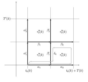
Figure 4: Loop $\delta_{4}$ is homotopic with loop $\alpha\cdot\alpha^{\prime}_{1}\cdot\beta_{2}^{-1}\cdot\beta_{1}^{\prime-1}\cdot\alpha_{1}^{-1}$, where $\alpha=\alpha_{1}\cdot\alpha_{2}$.

Four points $x_{l}(k)$, $l=0,1,2,3$ divide four loops $\lambda(k)$, $\lambda^{\prime}(k)$, $\gamma(k)$ and $\gamma^{\prime}(k)$ into eight semi-loops $\lambda_{l}(k)$, $\lambda_{l}^{\prime}(k)$, $\gamma_{l}(k)$ and $\gamma_{l}^{\prime}(k)$ which correspond to eight semi-loops $\alpha_{l}$, $\alpha_{l}^{\prime}$, $\beta_{l}$ and $\beta_{l}^{\prime}$, $l=1,2$ in the parallelogram of the periods. Of course we have $\lambda(k)=\lambda_{1}(k)\cdot\lambda_{2}(k)$, $\alpha=\alpha_{1}\cdot\alpha_{2}$, etc. We show that the fundamental group $\pi(\Gamma(k),x_{0}(k))$ is generated by closed loops which are appropriate compositions of these eight semi-loops. The fundamental group $\pi(\Gamma(k),x_{0}(k))$ is generated by homotopic classes of six loops with the base point at $x_{0}(k)$: $\lambda(k)$, $\lambda^{\prime}(k)$, and four loops $\sigma_{l}(k)$ encircling the singular points $s_{l}(k)$, $l=1,2,3,4$. They satisfy the following condition:

$$\sigma_{1}(k)\cdot\sigma_{2}(k)\cdot\sigma_{3}(k)\cdot\sigma_{4}(k)=\lambda(k)\cdot\lambda^{\prime}(k)\cdot\lambda(k)^{-1}\cdot\lambda^{\prime}(k)^{-1}.$$

We show that the loop $\sigma_{l}(k)$ has the same homotopic class as an appropriate composition of the semi-loops $\lambda_{l}(k)$, $\lambda_{l}^{\prime}(k)$, $\gamma_{l}(k)$ and $\gamma_{l}^{\prime}(k)$. For example:

$$[\sigma_{4}(k)]=[\lambda(k)\cdot\lambda^{\prime}_{1}(k)\cdot\gamma_{2}(k)^{-1}\cdot\gamma_{1}^{\prime}(k)^{-1}\cdot\lambda_{1}(k)^{-1}].$$

Let $\delta_{4}$ be the loop encircling $\tau_{4}(k)$ and let $\sigma_{4}(k)$ correspond to $\delta_{4}$. Then, we easily deduce that $\delta_{4}$ has the same homotopic class as $\alpha\cdot\alpha^{\prime}_{1}\cdot\beta_{2}^{-1}\cdot\beta_{1}^{\prime-1}\cdot\alpha_{1}^{-1}$, see Figure 4.

Thus, we show that all generators of the fundamental group $\pi(\Gamma(k),x_{0}(k))$ approach $\Omega$ as $k$ tends to 1. ∎

Now, we are ready to prove our main result.

Theorem 3.

If $C\neq 1$, $A=B=1$, ${\mathbf{L}}=(0,0,1)$, and $2\xi\neq{3}(1-C)$, then system  (2) considered on ${\mathcal{M}}^{6}$ does not admit an additional real meromorphic first integral functionally independent together with $H$ and $H_{5}$ in a neighbourhood of the phase curve $\Gamma_{1}$.

Proof.

Let us assume that such meromorphic integral exists in a real neighbourhood of the phase curve $\Gamma_{1}$. Then we can extend it to a complex meromorphic first integral in a complex neighbourhood $\widetilde{U}$ of $\Gamma_{1}$. Then, by Lemma 8 we find $\Gamma_{k}$ with $k$ close to 1 such that its fundamental group is generated by loops which lie entirely in $\widetilde{U}$. From the Ziglin Lemma 1 it follows that the monodromy group of the NVE (41) possesses an invariant. But the NVE (41) is a Fuchsian equation and thus if its monodromy group possesses an invariant, then its differential Galois group also possesses an invariant, see Theorem 3.17 in Braider:96:: . However, by Lemma 5 we show that the identity component of the differential Galois group of (47), and thus the identity component of the differential Galois group of (41), is $\mathrm{SL}(2,\mathbb{C})$. It follows that it does not possess an invariant, see Example 2.11(b) from Braider:96:: . A contradiction finishes the proof. ∎

6 Comments and Remarks

Although, as it is commonly believed, most systems are not integrable and integrable systems are extremely rare, the example considered in this paper shows that to prove the non-integrability one has to use rather involved techniques. Nevertheless, a proof of non-integrability of a system gives, in some sense, a negative result—the true aim is to find a non-trivial integrable system. From this point of view, the reader can wonder why we did not investigate carefully the case of the parameter values $2\xi=3(1-C)$ for which the necessary conditions for integrability are satisfied. As a matter of fact, for some time we believed that for these parameter values the system is integrable. With the help of the computer algebra we tried to find a polynomial or rational first integral of the system but we failed. For fixed values of $C$ we numerically generated the Poincaré cross sections of the system which evidently showed that the system is not integrable. Thus, our conjecture is that the system also is non-integrable for the case $2\xi=3(1-C)$. An analytic proof of this fact needs a separate investigation.

For $\xi=0$ Theorem 3 tells us that the problem of a symmetric rigid satellite in a circular orbit is not integrable for all values of $C\in(0,2)$ except $C=1$. This problem was also investigated in Maciejewski:01::i ; Maciejewski:01::j ; Audin:02:: where a proof of the same fact is given. However, in all these references as a particular solution a heteroclinic orbit was chosen and instead of transformation (43) another one was used. This leads to a more complicated form of the NVE.

7 Acknowledgements

We would like to thank Delphine Boucher, Juan J. Morales-Ruiz, Jacques-Arthur Weil, Carles Simó, Michael F. Singer and Felix Ulmer for discussions and help which allowed us to understand many topics related to this work. As usual, we thank Zbroja not only for her linguistic help. For the second author this research has been supported by a Maria Curie Fellowship of the European Community programme Human Potential under contract number HPMF-CT-2002-02031.

Appendix

Let us consider a linear second order differential equation with rational coefficients

$$w^{\prime\prime}+p(z)w^{\prime}+q(z)w=0,\qquad p(z),q(z)\in\mathbb{C}(z).$$ (82)

A point $z=c\in\mathbb{C}$ is a singular point of this equation if it is a pole of $p(z)$ or $q(z)$. A singular point is a regular singular point if at this point $\tilde{p}(z)=(z-c)p(z)$ and $\tilde{q}(z)=(z-c)^{2}q(z)$ are holomorphic. An exponent of equation (82) at point $z=z_{0}$ is a solution of the indicial equation

$$\rho(\rho-1)+p_{0}\rho+q_{0}=0,\qquad p_{0}=\tilde{p}(c),\quad q_{0}=\tilde{q}(c).$$

After changing the dependent variable $z\to 1/z$ equation (82) reads

$$w^{\prime\prime}+P(z)w^{\prime}+Q(z)w=0,\qquad P(z)=\frac{1}{z^{3}}p\left(\frac{1}{z}\right)+\frac{2}{z},\qquad Q(z)=\frac{1}{z^{4}}q\left(\frac{1}{z}\right).$$ (83)

We say that the point $z=\infty$ is a singular point for equation (82) if $z=0$ is a singular point of equation (82). Equation (82) is called Fuchsian if all its singular points (including infinity) are regular, see Whittaker:65:: ; Ince:44::

If one (non-zero) solution $w_{1}$ of equation (82) is Liouvillian, then all its solutions are Liouvillian. In fact, the second solution $w_{2}$, linearly independent from $w_{1}$, is given by

$$w_{2}=w_{1}\int\frac{1}{w_{1}^{2}}\exp\left[-\int p\right].$$

Putting

$$w=y\exp\left[\frac{1}{2}\int p\right]$$ (84)

into equation (82) we obtain its reduced form

$$y^{\prime\prime}=r(z)y,\qquad r(z)=-q(z)+\frac{1}{2}p^{\prime}(z)+\frac{1}{4}p(z)^{2}.$$ (85)

This change of variable does not affect the Liouvillian nature of the solutions. For equation (85) its differential Galois group ${\mathcal{G}}$ is an algebraic subgroup of $\mathrm{SL}(2,\mathbb{C})$. The following lemma describes all possible types of ${\mathcal{G}}$ and relates these types to forms of solution of (85), see Kovacic:86:: ; Morales:99:: .

Lemma 9.

Let ${\mathcal{G}}$ be the differential Galois group of equation (85). Then one of four cases can occur.

1. ${\mathcal{G}}$ is conjugated with a subgroup of the triangular group

   $${\mathcal{T}}=\left\{\begin{bmatrix}a&b\\ 0&a^{-1}\end{bmatrix}\;\biggl{|}\;a\in\mathbb{C}^{*},b\in\right\};$$

   in this case equation (85) has an exponential solution,

2. ${\mathcal{G}}$ is conjugated with a subgroup of

   $$D^{\dagger}=\left\{\begin{bmatrix}c&0\\ 0&c^{-1}\end{bmatrix}\;\biggl{|}\;c\in\mathbb{C}^{*}\right\}\cup\left\{\begin{bmatrix}0&c\\ c^{-1}&0\end{bmatrix}\;\biggl{|}\;c\in\mathbb{C}^{*}\right\},$$

   in this case equation (85) has a solution of the form $y=\exp\int\omega$, where $\omega$ is algebraic over $\mathbb{C}(z)$ of degree 2,

3. ${\mathcal{G}}$ is primitive and finite; in this case all solutions of equation (85) are algebraic,

4. ${\mathcal{G}}=\mathrm{SL}(2,\mathbb{C})$ and equation (85) has no Liouvillian solution.

When the first case occurs we say that equation (85) is reducible.

The Kovacic algorithm Kovacic:86:: allows to decide if an equation of the form (85) possesses a Liouvillian solution. Applying it we also obtain information about the differential Galois group of this equation. Now, beside the original formulation of this algorithm  we have its several versions and improvements and extensions to higher order equations Duval:89:: ; Duval:92:: ; Ulmer:96:: ; Singer:93:: ; Singer:95:: ; Hoeij:98:: ; Boucher:00::

Here we present a part of the Kovacic algorithm which allows to decide whether  (85) possesses a solution of the form $y=\exp\int\omega$, where $\omega$ is algebraic over $\mathbb{C}(z)$ of degree 1 or 2, or, in other words it gives an answer whether for equation (85) case 1 or 2 in Lemma 9 can occur. We used this part of the algorithm in Lemma 4 and Lemma 7. As our NVE is Fuchsian, we present the algorithm adopted for a Fuchsian equation because it is simpler than for a general case.

We write $r(z)\in\mathbb{C}(z)$ in the form

$$r(z)=\frac{s(z)}{t(z)},\qquad s(z),\,t(z)\in\mathbb{C}[z],$$

where $s(z)$ and $t(z)$ are relatively prime polynomials and $t(z)$ is monic. The roots of $t(z)$ are poles of $r(z)$. We denote $\Sigma^{\prime}:=\{c\in\mathbb{C}\,|\,t(c)=0\}$ and $\Sigma:=\Sigma^{\prime}\cup\{\infty\}$. The order $\operatorname{ord}(c)$ of $c\in\Sigma^{\prime}$ is equal to the multiplicity of $c$ as a root of $t(z)$, the order of infinity is defined by

$$\operatorname{ord}(\infty):=\max(0,4+\deg s-\deg t).$$

As we assumed, equation (85) is Fuchsian, so we have $\operatorname{ord}(c)\leq 2$ of $c\in\Sigma$. For each $c\in\Sigma^{\prime}$ we have the following expansion

$$r(z)=\frac{a_{c}}{(z-c)^{2}}+O\left(\frac{1}{z-c}\right),$$

and we define $\Delta_{c}=\sqrt{1+4a_{c}}$. For infinity we have

$$r(z)=\dfrac{a_{\infty}}{z^{2}}+O\left(\dfrac{1}{z^{3}}\right),$$

and we define $\Delta_{\infty}=\sqrt{1+4a_{\infty}}$.

Now we describe the Kovacic algorithm for the two cases mentioned.
Case I

Step I. For each $c\in\Sigma^{\prime}$ such that $\operatorname{ord}{c}=1$ we define $E_{c}=\{1\}$; if $\operatorname{ord}{c}=2$

$$E_{c}:=\left\{\frac{1}{2}\left(1+\Delta_{c}\right),\frac{1}{2}\left(1-\Delta_{c}\right)\right\}.$$

If $\operatorname{ord}{(\infty)}<2$ we put $E_{\infty}=\{0,1\}$; if $\operatorname{ord}{(\infty)}=2$ we define

$$E_{\infty}:=\left\{\frac{1}{2}\left(1+\Delta_{\infty}\right),\frac{1}{2}\left(1-\Delta_{\infty}\right)\right\}.$$

Step II. For each element $e$ in the Cartesian product

$$E:=E_{\infty}\times\prod_{c\in\Sigma^{\prime}}E_{c},$$

we compute

$$d(e):=1-\sum_{c\in\Sigma}e_{c}.$$

We select those elements $e\in E$ for which $d(e)$ is a non-negative integer. If there are no such elements equation (85) does not have an exponential solution and the algorithm stops here.

Step III. For each element $e\in E$ such that $d(e)=n\in\mathbb{N}_{0}$ we define

$$\omega(z)=\sum_{c\in\Sigma^{\prime}}\frac{e_{c}}{z-c},$$

and we search for a monic polynomial $P=P(z)$ of degree $n$ satisfying the following equation

$$P^{\prime\prime}+2\omega(z)P^{\prime}+(\omega^{\prime}(z)+\omega(z)^{2}-r(z))P=0.$$

If such polynomial exists, then equation (85) possesses an exponential solution of the form $y=P\exp\int\omega$, if not, equation (85) does not have an exponential solution.
Case II

Step I. For $c\in\Sigma^{\prime}$ such that $\operatorname{ord}{c}=1$ we define $E_{c}=\{4\}$; if $\operatorname{ord}{c}=2$

$$E_{c}:=\left\{2,2(1+\Delta_{c}),2(1-\Delta_{c})\right\}\cap\mathbb{Z}.$$

If $\operatorname{ord}{(\infty)}<2$ we put $E_{\infty}=\{0,2,4\}$; if $\operatorname{ord}{(\infty)}=2$ we define

$$E_{\infty}:=\left\{2,2(1+\Delta_{\infty}),2(1-\Delta_{\infty})\right\}\cap\mathbb{Z}.$$

Step II. If the Cartesian product

$$E:=E_{\infty}\times\prod_{c\in\Sigma^{\prime}}E_{c},$$

is empty then case 2 cannot occur and algorithm stops here. If it is not, then for $e\in E$ we compute

$$d(e):=2-\frac{1}{2}\sum_{c\in\Sigma}e_{c}.$$

We select those elements $e\in E$ for which $d(e)$ is a non-negative integer. If there are no such elements case 2 cannot occur and algorithm stops here.

Step III. For each element $e\in E$ such that $d(e)=n\in\mathbb{N}_{0}$ we define

$$\theta=\theta(z)=\frac{1}{2}\sum_{c\in\Sigma^{\prime}}\frac{e_{c}}{z-c},$$

and we search for a monic polynomial $P=P(z)$ of degree $n$ satisfying the following equation

$$P^{\prime\prime\prime}+3\theta P^{\prime\prime}+(3\theta^{2}+3\theta^{\prime}-4r)P^{\prime}+(\theta^{\prime\prime}+3\theta\theta^{\prime}+\theta^{3}-4r\theta-2r^{\prime})P=0.$$

If such a polynomial exists then equation (85) possesses a solution of the form $y=\exp\int\omega$, where

$$\omega^{2}-\psi\omega+\frac{1}{2}\psi^{\prime}+\frac{1}{2}\psi^{2}-r=0,\qquad\psi=\theta+\frac{P^{\prime}}{P}.$$

If we do not find such polynomial, then case 2 in Lemma 9 cannot occur.

References

- [1] V. I. Arnold. Mathematical Methods of Classical Mechanics. Graduate Texts in Mathematics. Springer-Verlag, New York, 1978.
- [2] Michèle Audin. Les systèmes hamiltoniens et leur intégrabilité. Cours Spécialisés. SMF et EDP Sciences, 2001.
- [3] Michèle Audin. La réduction symplectique appliquée á la non-intégrabilité du problème du satellite. 2002, preprint.
- [4] A. Baider, R. C. Churchill, D. L. Rod, and M. F. Singer. On the infinitesimal geometry of integrable systems. In Mechanics day (Waterloo, ON, 1992), volume 7 of Fields Inst. Commun., pages 5–56. Amer. Math. Soc., Providence, RI, 1996.
- [5] V. V. Beletskii. Motion of a Satellite about its Mass Center. Nauka, Moscow, 1965. In Russian.
- [6] V. V. Beletskii. Motion of a Satellite about its Mass Center in the Gravitational Field. Moscow University Press, Moscow, 1975. In Russian.
- [7] V. V. Beletskii and A. A. Hentov. Rotational Motion of a Magnetized Satellite. Moscow University Press, Moscow, 1985. In Russian.
- [8] Frits Beukers. Differential Galois theory. In From number theory to physics (Les Houches, 1989), pages 413–439. Springer, Berlin, 1992.
- [9] O. I. Bogoyavlenskii. Integrable cases of rigid-body dynamics and integrable systems on spheres . Izv. Akad. Nauk SSSR Ser. Mat., 49(5):899–915, 1985.
- [10] D. Boucher. Sur les équations différentielles linéaires paramétrées, une application aux systèmes hamiltoniens. PhD thesis, Universitè de Limoges, France, 2000.
- [11] F. de Brun. Rotation kring fix punkt. Öfvers. Kongl. Svenska Vetenskaps-Akad. Förhandl., 7:455–468, 1893.
- [12] G. N. Duboshin. Celestial Mechanics. Fundamental Problems and Methods. Nauka, Moscow, second, revised and enlarged edition, 1968. In Russian.
- [13] Anne Duval and Michèle Loday-Richaud. A propos de l’algoritme de Kovačic. Technical report, Université de Paris-Sud, Mathématiques, Orsay, France, 1989.
- [14] Anne Duval and Michèle Loday-Richaud. Kovačič’s algorithm and its application to some families of special functions. Appl. Algebra Engrg. Comm. Comput., 3(3):211–246, 1992.
- [15] E. L. Ince. Ordinary Differential Equations. Dover Publications, New York, 1944.
- [16] Irving Kaplansky. An introduction to differential algebra. Hermann, Paris, second edition, 1976. Actualités Scientifiques et Industrielles, No. 1251, Publications de l’Institut de Mathématique de l’Université de Nancago, No. V.
- [17] Jerald J. Kovacic. An algorithm for solving second order linear homogeneous differential equations. J. Symbolic Comput., 2(1):3–43, 1986.
- [18] Valerii V. Kozlov. Symmetries, Topology and Resonances in Hamiltonian Mechanics. Springer-Verlag, Berlin, 1996.
- [19] A. J. Maciejewski. A simple model of the rotational motion of a rigid satellite around an oblate planet. Acta Astronomica, 47:387–398, 1997.
- [20] A. J. Maciejewski. Non-integrability in gravitational and cosmological models. Introduction to Ziglin theory and its differential Galois extension. In A. J. Maciejewski and B. Steves, editors, The Restless Univers. Applications of Gravitational N-Body Dynamics to Planetary, Stellar and Galatic Systems, pages 361–385, 2001.
- [21] A. J. Maciejewski. Non-integrability of a certain problem of rotational motion of a rigid satellite. In H. Prȩtka-Ziomek, E. Wnuk, P. K. Seidelmann, and D. Richardson, editors, Dynamics of Natural and Artificial Celestial Bodies, pages 187–192. Kluwer Academic Publisher, 2001.
- [22] Andy R. Magid. Lectures on differential Galois theory, volume 7 of University Lecture Series. American Mathematical Society, Providence, RI, 1994.
- [23] J. E. Marsden and T. S. Ratiu. Introduction to Mechanics and Symmetry. Number 17 in Texts in Applied Mathematics. Springer Verlag, New York, Berlin, Heidelberg, 1999. second edition.
- [24] J. J. Morales-Ruiz. Kovalevskaya, Liapounov, Painlevé, Ziglin and the differential Galois theory. Regul. Chaotic Dyn., 5(3):251–272, 2000.
- [25] Juan J. Morales Ruiz. Differential Galois theory and non-integrability of Hamiltonian systems. Birkhäuser Verlag, Basel, 1999.
- [26] Juan J. Morales-Ruiz and Jean Pierre Ramis. Galoisian obstructions to integrability of Hamiltonian systems. I, II. Methods Appl. Anal., 8(1):33–95, 97–111, 2001.
- [27] H. Poincaré. Sur le problème des trois corps et les équations de la dynamique. Acta Math., 13:1–270, 1890.
- [28] Michael F. Singer. An outline of differential Galois theory. In Computer algebra and differential equations, pages 3–57. Academic Press, London, 1990.
- [29] Michael F. Singer and Felix Ulmer. Liouvillian and algebraic solutions of second and third order linear differential equations. J. Symbolic Comput., 16(1):37–73, 1993.
- [30] Michael F. Singer and Felix Ulmer. Necessary conditions for Liouvillian solutions of (third order) linear differential equations. Appl. Algebra Engrg. Comm. Comput., 6(1):1–22, 1995.
- [31] Alexei Tsygvintsev. La non-intégrabilité méromorphe du problème plan des trois corps. C. R. Acad. Sci. Paris Sér. I Math., 331(3):241–244, 2000.
- [32] Alexei Tsygvintsev. The meromorphic non-integrability of the three-body problem. J. Reine Angew. Math., 537:127–149, 2001.
- [33] Alexei Tsygvintsev. Sur l’absence d’une intégrale première méromorphe supplémentaire dans le problème plan des trois corps. C. R. Acad. Sci. Paris Sér. I Math., 333(2):125–128, 2001.
- [34] Felix Ulmer and Jacques-Arthur Weil. Note on Kovacic’s algorithm. J. Symbolic Comput., 22(2):179–200, 1996.
- [35] Mark van Hoeij, Jean-Francois Ragot, Felix Ulmer, and Jacques-Arthur Weil. Liouvillian solutions of linear differential equations of order three and higher. J. Symbolic Comput., 28:589–609, 1998.
- [36] E. T. Whittaker and G. N. Watson. A Treatise on the Analytical Dynamics of Particles and Rigid Bodies with an Introduction to the Problem of Three Bodies. Cambridge University Press, London, fourth edition, 1965.
- [37] S. L. Ziglin. Branching of solutions and non-existence of first integrals in Hamiltonian mechanics. I. Functional Anal. Appl., 16:181–189, 1982.
- [38] S. L. Ziglin. Branching of solutions and non-existence of first integrals in Hamiltonian mechanics. II. Functional Anal. Appl., 17:6–17, 1983.
- [39] S. L. Ziglin. On the absence of a real-analytic first integral in some problems of dynamics. Funktsional. Anal. i Prilozhen., 31(1):3–11, 95, 1997.