Wave turbulence in Bose-Einstein condensates

Abstract

The kinetics of nonequilibrium Bose-Einstein condensates are considered within the framework of the Gross-Pitaevskii equation. A systematic derivation is given for weak small-scale perturbations of a steady confined condensate state. This approach combines a wavepacket WKB description with the weak turbulence theory. The WKB theory derived in this paper describes the effect of the condensate on the short-wave excitations which appears to be different from a simple renormalization of the confining potential suggested in previous literature.

To Appear in Physica D

1 Introduction

Bose-Einstein condensate (BEC) was first observed in 1995 in atomic vapors of ⁸⁷Rb Anderson , ⁷Li Bradley and ²³Na Davis . Typically, the gas of atoms is confined by a magnetic trap Anderson , and cooled by laser and evaporative means. Although the basic theory for the condensation was known from the classical works of Bose Bose and Einstein Einstein , the experiments on BEC stimulated new theoretical work in the field (an excellent review of this material is given in Pitaevsky ).

A lot of theoretical results about condensate dynamics are based on the assumption that the condensate band can be characterized by some temperature $T$ and chemical potential $\mu$, the quantities which are clearly defined only for gases in thermodynamic equilibrium. Often, however, the condensation is so rapid that the gas is in a very nonequilibrium state and hence, one requires the use of a kinetic rather than a thermodynamic theory Gardiner ; Gardiner2 ; SV . An approach using the quantum kinetic equation was developed by Gardiner et al Gardiner ; Gardiner2 who used some phenomenological assumptions about the scattering amplitudes. Phenomenology is unavoidable in the general case due to an extreme dynamical complexity of quantum gases the atoms in which interact among themselves and exhibit wave-particle dualism. Most phenomenological assumptions are intuitive or arise from a physical analogy and are hard to validate (or to prove wrong) theoretically. In particular, it was proposed that the ground BEC states act onto the higher levels via an effective potential. In the present paper we are going to examine this assumption in a special case of large occupation numbers, i.e. when the system is more like a collection of interacting waves rather than particles and which allows a systematic theoretical treatment. In what follows we show systematically that such an assumption is not true for such systems. For dilute gases, with a large number of atoms at low temperatures, one obtains the Gross-Pitaevskii (GP) equation for the condensate order parameter Gross ; Pitaevsky1961 :

$$i\partial_{t}\psi+\triangle\psi-|\psi|^{2}\psi-U\psi=0,$$ (1)

where the potential $U$ is a given function of coordinate, see for example figure 1. We emphasize that the area of validity of GP equation is restricted to a narrow class of the low-temperature BEC growth experiments and the latest stages in other BEC experiments. However, we will study the GP equation because it provides an important limiting case for which one can rigorously test the phenomenological assumptions made for more general systems. We would like to abandon the approach where the system is artificially divided into a $T=0$ condensate state and a thermal “cloud” because this “cloud” in reality is far from the thermodynamic equilibrium and we believe that this fact affects the BEC dynaimcs in an essential way. As in many other non-equilibrium and turbulent systems, fluxes of the conserved quantities through the phase space are more relevant for the theory here than the temperature and the chemical potential. Performance of a thermodynamic theory here would be as poor as a description of waterfalls by a theory developed for lakes. Again, the GP equation is used in our work for both the ground and the excited states which limits our analysis only to the low temperature and high occupation number situations.

In fact the idea of using GP equation for describing BEC kinetics is not new and it goes back to work of Kagan et al SV , who used a kinetic equation for waves systematically derived from the GP equation ignoring the trapping potential and assuming turbulence to be spatially homogeneous ZMR85 . A similar method has been used to investigate optical turbulence DNPZ92 . Classical weak turbulence theory yields a closed kinetic equation for the long time behavior of the energy spectrum without having to make unjustifiable assumptions about the statistics of the processes ZLF ; Newell ; Ben ; NazarenkoNewell ; Newell68 ; LBN . Second, the kinetic equation admits classes of exact equilibrium solutions ZLF ; Z68a ; Z68b . These can be identified as pure Kolmogorov spectra ZMR85 ; DNPZ92 ; ZLF , namely equilibria for which there is a constant spectral flux of one of the invariants, the energy,

$$E=\int[|\nabla\psi|^{2}+\frac{1}{2}|\psi|^{4}]\,d{\bf x},$$

and the “number of particles”,

$$N=\int|\psi|^{2}\,d{\bf x}.$$

A very important property of the particle cascade is that it transfers the particles to the small $k$ values (inverse cascade). This transfer will lead to an accumulation at small $k$’s which is precisely the mechanism of the BE condensation, see figure 1. The energy cascade is toward high values of $k$ which eventually will lead to “spilling” over the potential barrier corresponding to an evaporative cooling, see figure 1. After the formation of strong condensate one can no longer use weak turbulence theory, as the weak turbulence theory assumes small amplitudes. However, one can reformulate the theory using a linearization around the condensate, (as oppose to linearization around the $0$ state), as in DNPZ92 . Consequently this changes the dominant system interactions from 4-wave to 3-wave processes.

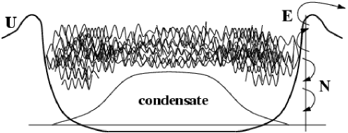
Figure 1: Turbulent cascades of energy $E$ and particle number $N$.

Kolmogorov-type energy distributions over the levels (scales) are dramatically different from any thermodynamic equilibrium distributions. Thus, the condensation and the cooling rates will also be significantly different from those obtained from theories based on the assumptions of a thermodynamic equilibrium and the existence of a Boltzmann distribution. As an example, a finite-time condensation was predicted by Kagan, Svistunov and Shlyapnikov SV , whose work was based on the theory of weak homogeneous turbulence.

However, application of the theory of homogeneous turbulence to the GP equation has its limitations. Indeed, when the external potential is not ignored in the GP equation, the turbulence is trapped and is, therefore, intrinsically inhomogeneous (e.g. a turbulent spot). Additional inhomogeneity of the turbulence arises because of the condensate, which in the GP equation case is itself coordinate dependent. This means, in particular, that the theory of homogeneous turbulence cannot describe the ground state effect onto the confining properties of the gas and thereby test the effective potential approach. The present paper is aimed at removing this pitfall via deriving an inhomogeneous weak turbulence theory.

The effects of the coordinate dependent potential and condensate can most easily be understood using a wavepacket (WKB) formalism that is applicable if the wavepacket wavelength $l$ is much shorter than the characteristic width of the potential well $L$,

$$\varepsilon=\frac{l}{L}\ll 1.$$

The coordinate dependent potential and the condensate distort the wavepackets so that their wavenumbers change. This has a dramatic effect on nonlinear resonant wave interactions because now waves can only be in resonance for a finite time. The goal of our paper is to use the ideas developed for the GP equation without the trapping potential and to combine them with the WKB formalism in order to derive a weak turbulence theory for a large set of random waves described by the GP equation.

Note that idea to combine the kinetic equation with WKB to describe weakly nonlinear dynamics of wave (or quantum) excitations is quite old and can be traced back to Khalatnikov’s theory of Bose gas (1952) and Landau’s theory of the Fermi fluids (1956), see e.g. in landafshits10 . It has also been widely used to describe kinetics of waves in plasmas, e.g. bbk ; tsit1 ; tsit2 ; zmrub . For plasmas, such a formalism was usually derived from the first principles. However, only phenomenological models based on an experimentally measured dispersion curves have been proposed so far for the superfluid kinetics. In this paper, we offer for the first time a consistent derivation starting from the GP equation which allows us to correct the existing BEC phenomenology at least for the special cases when the GP equation is applicable.

Technically, the most nontrivial new element of our theory appears through the linear dynamics (WKB) whereas modifications of the nonlinear part (the collision integral) are fairly straightforward. Thus, we start with a detailed consideration of the linear dynamics in section 2. Previously, linear excitations to the ground state were considered by Fetter fetter who used a test function approach to derive an approximate dispersion relation for these excitations. Fetter pointed out an uncertainty of the boundary conditions to be used at the ground state reflection surface. The WKB theory for BEC which is for the first time developed in the present paper allows an asymptotically rigorous approach which, among other things, allows to clarify the role of the ground state reflection surface. Indeed, as we will see in section 3, the WKB theory is essentially different in the case when the condensate ground state is weak and can be neglected from the case of strongly nonlinear ground state. No suitable WKB description exists for the intermediate case in which the linear and the nonlinear effects are of the same order. However, in the Thomas-Fermi regime the layer of the intermediate condensate amplitudes is extremely narrow due to the exponential decay of the amplitude beyond the ground state reflection surface. This allowed us to combine the two WKB descriptions into one by formally re-writing the equations in such a way that they are correct in the limits of both weak and strong condensate. These equations will be wrong in the thin layer of intermediate condensate amplitudes, but this will not have any effect on the overall dynamics of wavepackets because they pass this layer too quickly to be affected by it.

In section 4 for the first time we present a Hamiltonian formulation of the WKB equations and derive a cannonical Hamiltonian the form of which is general for all WKB systems and not only BEC. The Hamiltonian formulation is needed to prepare the scene for the weak turbulence theory. In section 5 we apply weak turbulence theory to write a closed kinetic equation for wave action. This kinetic equation has a coordinate dependence of the frequency delta functions. Notice that coordinate dependence of the wave frequency has a profound effect on the nonlinear dynamics. The resonant wave interactions can now take place only over a limited range of wave trajectories which makes such interactions similar to the collision of discrete particles.

2 Linear dynamics of the GP equation

We will now develop a WKB theory for small-scale wave-packets, described by a linearized GP equation, with and without the presence of a background condensate. As is traditional with any WKB-type method we assume the existence of a scale separation $\varepsilon\ll 1$, as explained in section 1. In this analysis we will take $l\sim 1$ so that any spatial derivatives of a given large-scale quantity (e.g. the potential $U$ or the condensate) are of order $\varepsilon$. The transition to WKB phase-space is achieved through the application of the Gabor transform nkd ,

$$\hat{g}(\vec{x},\vec{k},t)=\int f(\varepsilon^{*}|\vec{x}-\vec{x}_{0}|)\,\mathrm{e}^{i\vec{k}\cdot(\vec{x}-\vec{x}_{0})}\,g(\vec{x}_{0},t)\,d\vec{x}_{0},$$ (2)

where $f$ is an arbitrary function fastly decaying at infinity. For our purposes it will be sufficient to consider a Gaussian of the form

$$f(\vec{x})=\frac{1}{(2\pi)^{d}}\,e^{-x^{2}},$$

where $d$ is the number of space dimensions. The parameter $\varepsilon^{*}$ is small and such that $\varepsilon\ll\varepsilon^{*}\ll 1$. Hence, our kernel $f$ varies at the intermediate-scale. A Gabor transform can therefore be thought of as a localized Fourier transform, and in the limit $\epsilon^{*}\to 0$ becomes an exact Fourier transform. Physically, one can view a Gabor transform as a wavepacket distribution function over positions $\vec{x}$ and wavevectors $\vec{k}$.

2.1 Linear theory without a condensate

Linearizing the GP equation, to investigate the behavior of wavepackets $\psi$ without the presence of a condensate, we obtain the usual linear Schrödinger equation:

$$i\partial_{t}\psi+\triangle\psi-U\psi=0,$$ (3)

where $U$ is a slowly varying potential. Let us apply the Gabor transformation to (3). Note that the Gabor transformation commutes with the Laplacian, so that $\widehat{\Delta\Psi}=\Delta\hat{\Psi}$. Also note that

$$\widehat{U\Psi}\simeq U\hat{\Psi}+i(\nabla_{x}U)\nabla_{k}\hat{\Psi},$$

where we have neglected the quadratic and higher order terms in $\epsilon$ because $\Psi$ changes on a much shorter scale than the large scale function $U$. Combining the Gabor transformed equation with its complex conjugate we find the following WKB transport equation,

$$D_{t}|\hat{\psi}|^{2}=0,$$ (4)

where

$$D_{t}\equiv\partial_{t}+\dot{\vec{x}}\cdot\nabla+\dot{\vec{k}}\cdot\partial_{k},$$

represents the total time derivative along the wavepacket trajectories in phase-space. The ray equations are used to describe wavepacket trajectories in $(\vec{k},\vec{x})$ phase-space,

$$\dot{\vec{x}}=\partial_{k}\omega, \dot{\vec{k}}=-\nabla\omega.$$ (5)

The frequency $\omega$, in this case, is given by $\omega=k^{2}+U$, (again we use the notation $k=|\vec{k}|$). Equations (4) and (5) are nothing more than the famous Ehrenfest theorem from quantum mechanics. According to (5), the wavepackets will get reflected by the potential at points $r_{R}$ where $U(r_{R})=k^{2}_{max}$. We will now move on to consider linear wavepackets in the presence of a background condensate.

2.2 Wavepacket dynamics on a condensate background

One of the common assumptions in the BEC theory is that the presence of a condensate acts on the higher levels by just modifying the confining potential $U$, see for example GLBDZ98 . If this was the case, the linear dynamics would still be described by the Ehrenfest theorem with some new effective potential. We will show below that this is not the case.

Let us define the condensate $\psi_{0}$ as a nonlinear coordinate dependent solution of equation (1), with a lengthscale of the order of the ground state size (although it does not need to be exactly the same as the ground state). In what follows, we will use Madelung’s amplitude-phase representation for $\psi_{0}$, namely

$$\psi_{0}=\sqrt{\rho({\bf r})}\,e^{i\theta},$$ (6)

where ${\bf v}=2\nabla\theta$ is the macroscopic speed of the condensate. It is well known that in this representation $\rho$ obeys a continuity equation,

$$\rho_{t}+\hbox{div}({\rho{\bf v}})=0.$$ (7)

For future reference, one should note that the second term in this expression is $O(\epsilon^{2})$. Thus, $\rho_{t}$ is $O(\epsilon^{2})$ too and it must be neglected in the WKB theory which takes into account only linear in $\epsilon$ terms. We start by considering a small perturbation $\phi\ll 1$, such that

$$\psi=\psi_{0}(1+\phi).$$ (8)

Substituting (8) into (1) we find

$$i\partial_{t}\phi+\triangle\phi+2\frac{\nabla\psi_{0}}{\psi_{0}}\cdot\nabla\phi-\varrho\Big{(}\phi+\phi^{*}+2|\phi|^{2}+\phi^{2}+|\phi|^{2}\phi\Big{)}=0.$$ (9)

where $\varrho=\varrho(\vec{x})=|\psi_{0}|^{2}$ is a slowly varying condensate density.

In a similar manner to the previous subsection, the rest of this derivation consists of Gabor transforming (9), combining the result with its complex conjugate and finding a suitable waveaction variable such that the transport equation represents a conservation equation along the rays. Such a derivation is given in Appendix A. It yields to the following expression for the waveaction,

$$n({\bf k},x,t)=\frac{1}{2}\frac{\omega\rho}{k^{2}}\left|\widehat{\Re\phi}-\frac{ik^{2}}{\omega}\widehat{\Im\phi}\right|^{2},$$ (10)

where $\Re$ and $\Im$ mean the real and imaginary parts respectively. As usual, the transport equation takes the form of a conservation equation for waveaction along the rays,

$$D_{t}n(\vec{x},\vec{k},t)=0,$$ (11)

where

$$D_{t}\equiv\partial_{t}+\dot{\vec{x}}\cdot\nabla+\dot{\vec{k}}\cdot\partial_{k},$$ (12)

is the time derivative along trajectories

$$\dot{\vec{x}}=\partial_{k}\omega,\hskip 28.45274pt\dot{\vec{k}}=-\nabla\omega.$$ (13)

The frequency is given by the following expression,

$$\omega=k\sqrt{k^{2}+2\varrho}.$$ (14)

One can immediately recognize in (14) the Bogolubov’s formula Bogolubov1947 which was derived before for systems with a coordinate independent condensate and without a trapping potential. It is remarkable that presence of the potential $U$ does not affect the frequency so that expression (14) remains the same. Obviously, the dynamics in this case cannot be reduced to the Ehrenfest theorem with any shape of potential $U$. Therefore, an approach that models a condensate’s effect by introducing a renormalized potential would be misleading in this case.

3 Applicability of WKB descriptions

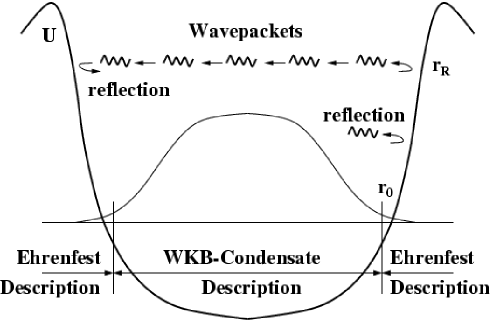
Figure 2: Regions of Applicability of WKB Descriptions.

In this section we will investigate the applicability of the above theory. Let us consider a condensate which is a solution of the eigenvalue problem $\partial_{t}\psi_{0}=-i\Omega\psi_{0}$. Therefore, the GP equation (1) becomes

$$\Omega\psi_{0}+\triangle\psi_{0}-\varrho\psi_{0}-U\psi_{0}=0.$$ (15)

3.1 Weak condensate case

Firstly, let us consider the case of a weak condensate so that the effect of the nonlinear term is small in comparison to the linear ones, $|\varrho\psi_{0}|\lesssim|\triangle\psi_{0}|$. Since $\Omega$ is a constant we observe that the Laplacian term acts to balance the external potential term (like in the linear Schrödinger equation) and the nonlinear term can be, at most, as big as the linear ones

$$\Omega\sim\frac{1}{r_{0}^{2}}\sim U(r_{0})\gtrsim\varrho,$$

where $r_{0}$ is the characteristic size of the condensate (it is defined as the condensate “reflection” point via the condition $\Omega=U(r_{0})$, see below).

Now for a WKB description to be valid we require $kr_{0}\gg 1$, i.e. we require the characteristic length-scale of our wavepackets to be a lot smaller than that of the large-scales. Using this fact we find

$$k^{2}\gg\frac{1}{r_{0}^{2}}\sim U(r_{0})\gtrsim\varrho.$$

Therefore, the condensate correction to the frequency, given by (14), is small. In other words the wavepacket does not “feel” the condensate. Indeed, from $k_{max}^{2}=U(r_{R})$ we have $U(r_{R})\gg U(r_{0})$ and this implies that $r_{R}\gg r_{0}$ (where $r_{R}$ is the wavepacket reflection point, see figure 2). Thus, the condensate in this case occupies a tiny space at the bottom of the potential well and hence does not affect a wavepacket’s motion. Therefore, a wavepacket moves as a “classical” particle described by the Ehrenfest equations (4) and (5). In fact, in this case it would be incorrect to try to describe the small condensate corrections via our WKB approach because these corrections are of order $\varrho\sim\varepsilon^{2}$ (the $\varepsilon^{2}$ terms being ignored in a WKB description).

3.2 Strong condensate case

Now we will consider a strong condensate such that

$$\Omega\cong U+\varrho\gg\frac{|\triangle\psi_{0}|}{|\psi_{0}|},$$ (16)

i.e. the $r$ dependence of the potential $U$ is now balanced by the nonlinearity. This is usually referred to as the Thomas-Fermi limit Pitaevsky . Wavepackets now “feel” the presence of a strong condensate if $\varrho\sim k^{2}$. We see that the WKB approach is applicable because

$$k^{2}\sim\varrho\gg\frac{1}{r_{0}^{2}}\sim\frac{|\triangle\psi_{0}|}{|\psi_{0}|}.$$

According to the ray equations $\omega$ is a constant along a wavepacket’s trajectory, so we can find the packet’s wavenumber from $k^{2}=\sqrt{\varrho^{2}+\omega^{2}}-\varrho$. One can see that $k^{2}$ remains positive for any value of $\varrho$ which means that the presence of the condensate does not lead to any new wavepacket reflection points (i.e. when $k$ takes a value of zero). Thus, turbulence is allowed to penetrate into the center of the potential well. However, the group velocity increases when the condensate becomes stronger, $\partial_{k}\omega\sim\sqrt{\rho}$. This means that the density of wavepackets decreases toward the center of well. Therefore, the condensate tends to push the turbulence away from the center, toward the edges of the potential trap.

To summarize, in the presence of a strong condensate we have two regions of applicability for our WKB descriptions, see figure 2. Wavepackets at a position $r<r_{0}$, in the central region of the potential well will evolve according to the WKB-condensate description (10) - (14). The Laplacian term only becomes important for $r>r_{0}$ where $\varrho$ is exponentially small. In this case the Ehrenfest description is appropriate. It will be shown in the next section that these two WKB descriptions can be combined into a single set of formulae.

3.3 Unified WKB description

It is interesting that taking the limit of zero condensate amplitude in the waveaction (10) results in the waveaction $\frac{1}{2}|\hat{\Psi}|^{2}$ of the Ehrenfest equation (4) which corresponds to the regime without condensate,

$$\lim\limits_{\rho\to 0}n({\bf k},x,t)\to\frac{1}{2}\rho\left|\widehat{\phi}\right|^{2}=\frac{1}{2}|\hat{\Psi}|^{2}.$$

On the other hand, $\lim\limits_{\rho\to 0}\omega\to k^{2}$ which is different from the Ehrenfest expression $\omega=k^{2}+U$. Thus, one cannot recover the non-condensate (Ehrenfest) description by just taking the limit of zero condensate amplitude in (10), (11) and (14). However, one can easily write a unified WKB description which will be valid with or without condensate by simply adding $U+\rho$ to the frequency (14). Indeed, for strong condensate $U+\rho$=const and, therefore, it does not alter the ray equations (which contain only derivatives of $\omega$). On the other hand, such an addition allows us to obtain the correct expression

$$\omega=k^{2}+U,$$

in the limit $\rho\to 0$. Summarizing, we write the following equations of the linear WKB theory which are valid with or without the presence of a condensate,

$$D_{t}n(\vec{x},\vec{k},t)=0,$$ (17)

where

$$n({\bf k},x,t)=\frac{1}{2}\frac{\omega\rho}{k^{2}}\left|\widehat{\Re\phi}-\frac{ik^{2}}{\omega}\widehat{\Im\phi}\right|^{2},$$ (18)

is the waveaction and

$$D_{t}\equiv\partial_{t}+\dot{\vec{x}}\cdot\nabla+\dot{\vec{k}}\cdot\partial_{k},$$ (19)

is the full time derivative along trajectories and

$$\dot{\vec{x}}=\partial_{k}\omega,\hskip 28.45274pt\dot{\vec{k}}=-\nabla\omega,$$ (20)

are the ray equations with

$$\omega=k\sqrt{k^{2}+2\varrho}+U+\rho.$$ (21)

Formula (21) is an important and nontrivial result which can be obtained neither from existing general facts about the WBK formalism nor from the linear theory of homogeneous systems.

4 Weakly nonlinear GP equation

The derivation for the description of the nonuniform turbulence found in a BEC system consists of a amalgamation of a WKB method, for the description of the linear dynamics, and a standard weak turbulence theory (see e.g. DNPZ92 ), with the noted modification that Gabor transforms are used instead of Fourier ones. We will now demonstrate the general ideas of such a derivation for the simple case of system where no condensate is present.

Consider the Gabor transformation of (1):

$$i\partial_{t}\hat{\psi}+\triangle\hat{\psi}-\widehat{|\psi|^{2}\psi}-U\hat{\psi}+i{\bf}(\nabla_{x}U)\nabla_{k}\hat{\psi}=0.$$ (22)

To calculate the $\widehat{|\psi|^{2}\psi}$ term let us first separate the Gabor transform into its correspondingly fast and slow spatial parts,

$$\hat{\psi}(\vec{x},\vec{k},t)=\underbrace{a(\vec{x},\vec{k},t)}_{\mbox{slow}}\underbrace{e^{i{\vec{k}}\cdot{\vec{x}}}}_{\mbox{fast}}.$$ (23)

Now by using the inverse Gabor transform

$$g(x,t)=\int\hat{g}(\vec{x},\vec{k},t)\,d{\vec{k}},$$ (24)

we find

$$\widehat{|\psi|^{2}\psi}=e^{i{\vec{k}}\cdot{\vec{x}}}\int f (\vec{x}-\vec{x}_{0})\,e^{i\vec{x}_{0}\cdot(\vec{k}_{3}+\vec{k}_{2}-\vec{k}_{1}-\vec{k})}$$

$$\times a^{*}(\vec{k}_{1},\vec{x}_{0})a(\vec{k}_{2},\vec{x}_{0})a(\vec{k}_{3},\vec{x}_{0})\,d{\vec{x}_{0}}d{\vec{k}_{1}}d{\vec{k}_{2}}d{\vec{k}_{3}}.$$

Note that the slow amplitudes $a$ do not change much over the characteristic width of the function $f$ and hence their argument ${\vec{x_{0}}}$ can be replaced by ${\vec{x}}$. Therefore, we can approximate (LABEL:stuff1) by

$$\widehat{|\psi|^{2}\psi}\simeq\frac{e^{i{\vec{k}}\cdot{\vec{x}}}}{(2\pi)^{3d/2}}\int F (\vec{k}_{3}+\vec{k}_{2}-\vec{k}_{1}-\vec{k})$$

$$\times a^{*}(\vec{k}_{1},\vec{x})a(\vec{k}_{2},\vec{x})a(\vec{k}_{3},\vec{x})\,d{\vec{k}_{1}}d{\vec{k}_{2}}d{\vec{k}_{3}}.$$

Here $F(\vec{k})$ is the Fourier transform of $f(\vec{x})$. Note that for the spatially homogeneous systems, $\epsilon^{*}\to 0$, $F(\vec{k})$ is just a delta function,

$$\lim\limits_{\epsilon^{*}\to 0}F(\vec{k})\to\delta(\vec{k}).$$

After dropping terms proportional to $\triangle a$, equation (22) then becomes

$$\partial_{t}a(\vec{k},\vec{x})=-2\vec{k}\cdot\nabla a(\vec{k},\vec{x})$$

$$-i(k^{2}+\vec{k}\cdot(\nabla_{x})) a(\vec{k},\vec{x})-(\nabla_{x}U)(\nabla_{k}a(\vec{k},\vec{x}))$$

$$-\int F(\vec{k}_{3}+\vec{k}_{2} -\vec{k}_{1}-\vec{k})\,a^{*}(\vec{k}_{1},\vec{x})a(\vec{k}_{2},\vec{x})a(\vec{k}_{3},\vec{x})\,d{\vec{k}_{1}}d{\vec{k}_{2}}d{\vec{k}_{3}}.$$

This is the master equation formulating the nonlinear dynamics in terms of the Gabor amplitudes. This can serve as a starting point for the statistical averaging which in turn leads to the weak turbulence formalism. Note that this equation can be written in Hamiltonian form,

$$i\frac{\partial}{\partial t}a_{{\bf k},{\bf x}}=\frac{\delta H}{\delta a_{{\bf x},{\bf k}}^{*}},$$ (28)

with a Hamiltonian function

$$H=\int(\omega_{k,x}-{\bf x}\cdot \nabla_{x}\omega_{k,x})|a_{k,x}|^{2}$$

$$+\frac{i}{2}(\nabla_{x} \omega_{k,x})(a_{k,x}^{*}\nabla_{k}a_{k,x}-a_{k,x}\nabla_{k}a^{*}_{k,x})$$

$$+\frac{i}{2} (\nabla_{k}\omega_{k,x})(a_{k,x}\nabla_{x}a_{k,x}^{*}-a_{k,x}^{*}\nabla_{x}a_{k,x})\,d{\bf k}d{\bf x}$$

$$+\int F({\bf k_{3}}+{\bf k_{2}} -{\bf k_{1}}-{\bf k})$$

$$a^{*}({\bf k_{1}} ,{\bf x})a({\bf k_{2}},{\bf x})a({\bf k_{3}},{\bf x})a({\bf k_{4}},{\bf x})\,d{\vec{k}_{1}}d{\vec{k}_{2}}d{\vec{k}_{3}}d{\vec{k}_{4}},$$

where $\omega_{k,x}=k^{2}+U(x)$. In fact, such a Hamiltonian description can be derived directly, in terms of the Gabor amplitudes, from the Hamiltonian formulation of the original GP equation (see Appendix B).

If a condensate is present in the system, one can also re-write the equations in a Hamiltonian form with an identical quadratic part. That is, with $a$ being replaced by the normal amplitude, and $\omega$ by the frequency of waves, found in the presence of the condensate. It appears that the quadratic part of the Hamiltonian (LABEL:ham) is generic in the WKB context. Indeed, let us consider a typical Hamiltonian for linear waves in weakly inhomogeneous media papaLvov expressed in terms of Fourier amplitudes $a_{\bf q_{1}}$ and $a^{*}_{\bf q_{1}}$

$${\cal H}=\int\Omega({\bf q_{1}},{\bf q})\,a_{\bf q_{1}}a^{*}_{\bf q_{1}}\,d{\bf q}d{\bf q_{1}},$$ (30)

with a hermitian kernel $\Omega({\bf q_{1}},{\bf q})=\Omega({\bf q},{\bf q_{1}})$ which is strongly peaked at ${\bf q}-{\bf q_{1}}=0$. As we will show in a separate paper naz-lvov , this Hamiltonian can be represented in terms of the Gabor transforms as

$$H=\int(\omega_{\vec{k},\vec{x}}-{\bf x}\cdot \nabla_{x}\omega_{\vec{k},\vec{x}})|a_{k,x}|^{2}$$

$$+\frac{i}{2}(\nabla_{x} \omega_{\vec{k},\vec{x}})(a_{k,x}^{*}\nabla_{k}a_{k,x}-a_{k,x}\nabla_{k}a^{*}_{k,x})$$

$$+\frac{i}{2} (\nabla_{k}\omega_{\vec{k},\vec{x}})(a_{k,x}\nabla_{x}a_{k,x}^{*}-a_{k,x}^{*}\nabla_{x}a_{k,x})\,d{\bf k}d{\bf x},$$ (31)

where $a_{kx}$ are the Gabor coefficients, and $\omega_{\vec{k}\vec{x}}$ is the position dependent frequency, related to $\Omega({\bf q},{\bf q_{1}})$ via

$$\omega_{\vec{k},\vec{x}}=\int e^{-2i\vec{q}\cdot\vec{x}}\,\Omega(\vec{k},\vec{k}+2\vec{q})\,d\vec{q}.$$ (32)

Actually, such an expression is a canonical form, even for a much broader class of Hamiltonians that correspond to a significant class of linear equations with coordinate dependent coefficients naz-lvov . That is,

$${\cal H}=\int[A({\bf q_{1}},{\bf q})\,a_{\bf q_{1}}a^{*}_{\bf q}\,B({\bf q_{1}},{\bf q})\,a_{\bf q_{1}}a_{\bf-q}+c.c.]\,d{\bf q}d{\bf q_{1}},$$ (33)

where functions $A$ and $B$ peaked at ${\bf q}-{\bf q_{1}}=0$.

5 Weak turbulence for inhomogeneous systems

Now, by analogy with homogeneous weak turbulence, we define the waveaction spectrum as

$$n_{\vec{k},\vec{x}}=\langle|a(\vec{k},\vec{x})|^{2}\rangle/F(0),$$

where averaging is performed over the random initial phases. Note that this definition is slightly different to the usual definition of the turbulence spectrum in homogeneous turbulence, i.e. the definition constructed from Fourier transforms, $n_{\vec{k}}\,\delta(\vec{k}-\vec{k}^{\prime})=\langle a(\vec{k})a(\vec{k}^{\prime})\rangle$. Indeed, a Gabor transform can be viewed as a finite-box Fourier transform, where $\vec{k}=\vec{k}^{\prime}$ in the definition of the spectrum and one replaces $\delta(\vec{k}-\vec{k}^{\prime})$ with the box volume $F(0)$.

Multiplying (LABEL:morestuff2) by $a^{*}(\vec{k},\vec{x})$ and combining the resulting equation with its complex conjugate, we get a generalization of (4):

$$D_{t}n_{\vec{k},\vec{x}}=-2\Im\int F (\vec{k}+\vec{k}_{1}-\vec{k}_{2}-\vec{k}_{3})$$

$$\times\langle a^{*}(\vec{k},\vec{x})a^{*}(\vec{k}_{1},\vec{x})a(\vec{k}_{2},\vec{x})a(\vec{k}_{3},\vec{x})\rangle\,d{\bf k_{1}}d{\bf k_{2}}d{\bf k_{3}},$$

with $D_{t}\equiv\partial_{t}+\dot{\vec{x}}\cdot\nabla+\dot{\vec{k}}\cdot\partial_{k}$. Note, that in the case of homogeneous turbulence, using the random phase assumption, in the above equation, would lead to the RHS becoming zero. This means that the nontrivial kinetic equation appears only in higher orders of the nonlinearity. For the inhomogeneous case, the nontrivial effect of the nonlinearity appears even at this (second) order. This can be seen via a frequency correction which, in turn, modifies the wave trajectories. This effect was considered by Zakharov et al zmrub and it is especially important in systems where such frequency corrections result in modulational instabilities followed by collapsing events. In our case the nonlinearity is “defocusing” and, therefore, such an effect is less important. Indeed, in what follows we will neglect this effect as, at sufficiently small ratios of the inhomogeneity and turbulence intensity parameters, $\epsilon\ll\phi^{2}$, wave collision events are a far more dominant process.

Let us introduce notations

$$I^{kk_{1}}_{k_{2}k_{3}}\equiv\langle a^{*}(\vec{k},\vec{x})a^{*}(\vec{k}_{1},\vec{x})a(\vec{k}_{2},\vec{x})a(\vec{k}_{3},\vec{x})\rangle,$$

and

$$I^{kk_{1}k_{2}}_{k_{3}k_{4}k_{5}}\equiv\langle a^{*}(\vec{k},\vec{x})a^{*}(\vec{k}_{1},\vec{x})a^{*}(\vec{k}_{2},\vec{x})a(\vec{k}_{3},\vec{x})a(\vec{k}_{4},\vec{x})a(\vec{k}_{5},\vec{x})\rangle.$$

Then, we have the following equation for the 4th-order moment,

$$D_{t}I^{k_{1}^{\prime}k_{2}^{\prime}}_{k_{3}^{\prime}k_{4}^{\prime}}=i(\tilde{\omega}_{k^{\prime}_{1}}+\tilde{\omega}_{k_{2}^{\prime}}-\tilde{\omega}_{k_{3}^{\prime}}-\tilde{\omega}_{k_{4}^{\prime}}) I^{k^{\prime}_{1}k_{2}^{\prime}}_{k_{3}^{\prime}k_{4}^{\prime}}$$

$$+\int\Big{(}I^{k_{2}k_{3}k_{2}^{\prime}}_{k_{1}k_{3}^{\prime}k_{4}^{\prime}}F(\vec{k}_{1}^{\prime}+\vec{k}_{1}-\vec{k}_{2} -\vec{k}_{3})$$

$$+I^{k_{1}^{\prime}k_{2}k_{3}}_{k_{1}k_{3}^{\prime}k_{4}^{\prime}}F(\vec{k}_{2}^{\prime}+\vec{k}_{1} -\vec{k}_{2}-\vec{k}_{3})$$

$$-I^{k_{1}^{\prime}k_{2}^{\prime}k_{1}}_{k_{4}^{\prime}k_{2}k_{3}}F(\vec{k}_{3}^{\prime} +\vec{k}_{1}-\vec{k}_{2}-\vec{k}_{3})$$

$$-I^{k_{1}^{\prime}k_{2}^{\prime}k_{1}}_{k_{3}^{\prime}k_{2}k_{3}} F(\vec{k}_{4}^{\prime}+\vec{k}_{1}-\vec{k}_{2}-\vec{k}_{3})\,\Big{)}dk_{1}dk_{2}dk_{3},$$

where we denote $\tilde{\omega}_{k}=k^{2}+(\vec{k}\cdot\nabla_{x}U)$. Note that the first two terms on the RHS of this equation can be obtained one from another by exchanging $\vec{k}_{1}^{\prime}$ and $\vec{k}_{2}^{\prime}$, whereas the last two terms – by exchanging $\vec{k}_{3}^{\prime}$ and $\vec{k}_{4}^{\prime}$. To solve this equation, one can use the random phase assumption which is standard for the derivation of a weak homogeneous turbulence theory and which allows one to express the 6th-order moment in terms of the 2nd-order correlators. For homogeneous turbulence, the validity of this assumption was examined by Newell et al NazarenkoNewell ; Newell_ann who showed that initially Gaussian turbulence (characterized by random independent phases) remains Gaussian for the energy cascade range whereas in the particle cascade range deviations from Gaussianity grow toward low $k$ values. However, these deviations remain small over a large range of $k$ for small initial amplitudes and the random phase assumption can be used for these scales. Note that the deviations from Gaussianity at low $k$ correspond to the physical process of building a coherent condensate state. The results of NazarenkoNewell ; Newell_ann obtained for homogeneous GP turbulence will hold for trapped turbulence too because inhomogeneity has a neutral effect on the phase correlations. Indeed, according to the linear WKB equations the phases propagate unchanged along the rays. Thus we write

$$I^{123}_{456}\approx n_{1}n_{2}n_{3}\Big{(}F^{3}_{4}(F^{2}_{5}F^{1}_{6}+F^{1}_{5}F^{2}_{6})+ F^{3}_{5} (F^{2}_{6}F^{1}_{4}+F^{2}_{4}F^{1}_{6})$$

$$+ F^{3}_{6}(F^{1}_{5}F^{2}_{4}+F^{1}_{4}F^{2}_{5})\Big{)},$$

here we have used the shorthand notations, $F^{1}_{2}\equiv F(0)\,\delta(\vec{k}_{1}-\vec{k}_{2})$ and $I^{123}_{456}=I^{k_{1}k_{2}k_{3}}_{k_{4}k_{5}k_{6}}$. Using this expression in (LABEL:ef4m) we have

$$\frac{D}{Dt}I^{k_{1}k_{2}}_{k_{3}k_{4}}= i (\omega_{k_{1}}+\omega_{k_{2}}-\omega_{k_{3}}-\omega_{k_{4}})I^{k_{1}k_{2}}_{k_{3}k_{4}}$$

$$+ 2\left(n_{k_{3}}n_{k_{4}}(n_{k_{1}}+n_{k_{2}})-n_{k_{1}}n_{k_{2}}(n_{k_{3}}+n_{k_{4}})\right).$$

Notice that the $\tilde{\omega}_{k}$ terms get replaced by $\omega_{k}$, since the $(\vec{k}\cdot\nabla_{x}U)$ terms drop out on the resonant manifold. Let us integrate this equation over the period $T$ which is less than both the slow WKB time $1/\epsilon$ and the nonlinear time $1/\sigma^{4}$. Then, one can ignore the time dependence in $n_{k}$ on the RHS of the above equation and we can take $\dot{k}=-\nabla U=const$ on the LHS.

The resulting equation can be easily integrated along the characteristics (rays) which in the limit $\omega T\to\infty$ gives

$$I^{k_{1}k_{2}}_{k_{3}k_{4}}=-2[n_{k_{3}}n_{k_{4}}(n_{k_{1}}n_{k_{2}})-n_{k_{1}}n_{k_{2}}(n_{k_{3}} +n_{k_{4}})]$$

$$\delta(\omega_{k_{1}}+\omega_{k_{2}} -\omega_{k_{3}}-\omega_{k_{4}}).$$ (37)

Note that to derive a similar expression in the theory of homogeneous weak turbulence one usually introduces an artificial “dissipation” to circumvent the pole and to get the correct sign in front of the delta function (see e.g. ZLF ). The roots of this problem can be found even at the level of the linear dynamics, where the use of Laplace (rather than Fourier) transforms provides a mathematical justification for the introduction of such a dissipation. However, in our case there is no need for us to introduce such a dissipation because inhomogeneity removes the degeneracy in the system. Substituting (37) into (5) we get the main equation describing weak turbulence, the four-wave kinetic equation

$$D_{t}n_{k}=\frac{1}{\pi}\int n_{k} n_{1}n_{2}n_{3}\left(\frac{1}{n_{k}}+\frac{1}{n_{1}}-\frac{1}{n_{2}}-\frac{1}{n_{3}}\right)\delta\left(\vec{k}+\vec{k}_{1}-\vec{k}_{2}-\vec{k}_{3}\right)$$

$$\delta\left(\omega_{k}({\bf x})+\omega_{1}({\bf x})-\omega_{2}({\bf x})-\omega_{3}({\bf x})\right)\,d\vec{k}_{1}d\vec{k}_{2}d\vec{k}_{3},$$

where,

$$D_{t}\equiv\partial_{t}+\dot{\vec{x}}\cdot\nabla+\dot{\vec{k}}\cdot\partial_{k}, \dot{\vec{x}}=\partial_{k}\omega,\,\,\,\,\,\,\,\dot{\vec{k}}=-\nabla\omega.$$

We can see that the main difference between the kinetic equation for inhomogeneous media and homogeneous turbulence SV ; ZMR85 ; DNPZ92 ; Newell68 is that the partial time derivative on the LHS is replaced by the full time derivative along the rays. Further, the frequency $\omega$ and spectrum $n$ are now functions not only of the wavenumber but also of the coordinate.

The same is true for the case when the ground state condensate is important for the wave dynamics DNPZ92 . The main interaction mechanism now become three wave interactions, with the kinetic equation

$$D_{t}n = \pi\int|V_{kk_{1}k_{2}}|^{2}\,f_{k12}\,\delta_{{{\bf k}-\bf{k_{1}}-\bf{k_{2}}}}\,\delta_{\omega_{{\bf k}}-\omega_{{\bf{k_{1}}}}-\omega_{{\bf{k_{2}}}}}d{\bf k}_{1}d{\bf k}_{2}\,$$ (39)

$$- 2\pi\int\,|V_{k_{1}kk_{2}}|^{2}\,f_{1k2}\,\delta_{{{\bf k_{1}}-\bf{k}-\bf{k_{2}}}}\,\delta_{{\omega_{{\bf k_{1}}}-\omega_{{\bf{k}}}-\omega_{{\bf{k_{2}}}}}}\,d{\bf k}_{1}d{\bf k}_{2}\,,$$

where $f_{k12}=n_{{\bf k_{1}}}n_{{\bf k_{2}}}-n_{{\bf k}}(n_{{\bf k_{1}}}+n_{{\bf k_{2}}})\,$. Here, $n_{k}$, $D_{t}$ and $\omega$ are given by expressions (18), (19) and (21) respectively and the expression for the interaction coefficient $V_{kk_{1}k_{2}}$ can be found in DNPZ92 . Three-wave interactions always dominate over the four-wave process when $\rho\sim k^{2}$ (because $k\sim 1$ and $n\ll 1)$. In the case $\rho\ll k^{2}$, the relative importance of the three-wave and the four-wave processes can be established by comparing the characteristic times associated with these processes. The characteristic time of the three wave interactions for $\rho\ll k^{2}$ is

$$\tau_{3w}=k^{2-d}/\varrho n.$$

Thus, the 3-wave process will dominate the 4-wave one if the condensate is stronger than the waves, i.e. if $\varrho>nk^{d}\sim\phi^{2}$.

6 Summary

In this paper, we developed a theory of weak inhomogeneous wave turbulence for BEC systems. We started with the GP equation and derived a statistical theory for the BEC kinetics which, in particular, describes states which are very far from the thermodynamic equilibrium. Such nonequilibrium states take the form of wave turbulence which is essentially inhomogeneous due to the fact that the BEC is trapped by an external field. There are two main new results in this paper. First of all, we have described the effect of the inhomogeneous ground state on the linear wave dynamics and, in particular, we have shown that such an effect cannot be modeled by renormalizing the trapping potential as it was previously suggested in literature. This was done by deriving a consistent WKB theory based on the scale separation between the ground state and the waves. Our results show that the condensate “mildly” pushes the wave turbulence away from the center but it can never reflect it (as an external potential would). Note that we established this result only for the limit of large occupation numbers described by the GP equation and this, in principle, does not rule out a possibility that the the renormalized potential approach can still be valid in the opposite limit of small occupation numbers. Secondly, we showed that the kinetic equation for trapped waves generalizes, and one can combine the linear WKB theory and the theory of homogeneous weak turbulence in a straightforward manner. Namely, the partial time derivative on the LHS of the kinetic equation is replaced by the full time derivative along the wave rays, while the frequency and the spectrum on the RHS now become functions of coordinate. A suitable definition for the coordinate dependent spectrum is given by using the Gabor transforms instead of Fourier transforms. It is important to notice that the coordinate dependence of the wave frequency has a profound effect on the nonlinear dynamics. The resonant wave interactions can now take place only over a limited range of wave trajectories which makes such interactions similar to the collision of discrete particles.

Similarly to the case of homogeneous turbulence considered in DNPZ92 , the presence of a condensate changes the resonant wave

interactions from four-wave to three-wave if the condensate intensity exceeds that of the waves. A distinct feature of the inhomogeneous turbulence trapped by a potential is that if the three-wave regime is dominant in the center of the potential well, it is likely to be suddenly replaced by a four-wave dynamics when one moves out of the center beyond the condensate reflection points where the condensate intensity is decaying exponentially fast. Thus the same wavepacket can alternate between three-wave and four-wave interactions, with other wavepackets, as it travels back and forth between its reflection points in the potential well. (The wavepacket reflection points being further away from the center than the condensate’s own reflection points).

Appendix A: derivation WKB equations in presence of a condensate

Let us split $\phi$ into its real and imaginary parts $a=\Re\phi$ and $b=\Im\phi$. Then the equation (9) splits into two coupled equations

$$\partial_{t}a +\triangle b+2\vec{v}\cdot\nabla a+\frac{\nabla\varrho}{\varrho}\cdot\nabla b+\rho(2ab+b(a^{2}+b^{2}))=0,$$ (40)

$$\partial_{t}b -\triangle a+2a\varrho+2\vec{v}\cdot\nabla b-\frac{\nabla\varrho}{\varrho}\cdot\nabla a+{\varrho}(3a^{2}+b^{2}+a(a^{2}+b^{2}))=0,$$ (41)

where we have used the fact that $\frac{\nabla\psi_{0}}{\psi_{0}}=\frac{\nabla\varrho}{2\varrho}+\frac{i}{2}\vec{v}$, which follows from (6).

Gabor transforming our two coupled equations (40) and (41) and using Taylor series to represent large-scale quantities,

$$\varrho(\vec{x}_{0})=\varrho(\vec{x})+(\vec{x}_{0}-\vec{x})\cdot\nabla\varrho(\vec{x})+O(\varepsilon^{2}),$$

we find

$$\partial_{t}\hat{a}+\triangle\hat{b}+\frac{\nabla\varrho}{\varrho}\cdot\nabla\hat{b}+\vec{v}\cdot\nabla\hat{a} +{\cal G}\left[\rho(2ab+b(a^{2}+b^{2}))\right]=0,$$ (42)

$$\partial_{t}\hat{b}-\triangle\hat{a}-{\bf}\frac{\nabla\varrho}{\varrho}\cdot\nabla\hat{a}+2{\bf}\vec{v}\cdot\nabla\hat{b} +2\varrho\hat{a}+2i{\bf}\nabla\varrho\cdot\partial_{k}\hat{a}$$

$$+{\cal G}\left[(\varrho(3a^{2}+b^{2}+a(a^{2}+b^{2})))\right]=0.$$ (43)

Where ${\cal G}[f(x)]$ is the Gabor transform of $f(x)$. We have kept only $O(\varepsilon)$ terms and neglected the $O(\varepsilon^{2})$ and higher order terms. For generality, we have kept the nonlinear term.

The $\epsilon^{0}$ order -

As in all WKB based theories we first derive a linear dispersion relationship from the lowest order terms. At zeroth order in ${\bf\epsilon}$, the spatial derivative of a Gabor transform is $\nabla\hat{a}=i\vec{k}\hat{a}$ which is similar to the corresponding rule in Fourier calculus. Then, at the lowest order, equations (42) and (43) become

$$\partial_{t}\hat{a} -k^{2}\hat{b}=0,$$ (44)

$$\partial_{t}\hat{b} +k^{2}\hat{a}+2\varrho\hat{a}=0.$$ (45)

These two linear coupled equations make up an eigenvalue problem. Diagonalizing these equations we obtain

$$\partial_{t}\lambda=+i\omega\lambda, \partial_{t}\mu=-i\omega\mu.$$

Correspondingly, we find the eigenvectors

$$\lambda=\frac{1}{2}\left(\hat{a}-\frac{ik^{2}}{\omega}\hat{b}\right), \mu=\frac{1}{2}\left(\hat{a}+\frac{ik^{2}}{\omega}\hat{b}\right),$$ (46)

or, re-arranging for $\hat{a}$ and $\hat{b}$

$$\hat{a}=\lambda+\mu, \hat{b}=\frac{i\omega}{k^{2}}(\lambda-\mu).$$ (47)

The eigenvalues are given by the dispersion relationship,

$$\omega^{2}=k^{2}(k^{2}+2\varrho),$$ (48)

which is identical to the famous Bogoliubov form Bogolubov1947 which was also obtained for waves on a homogeneous condensate in the weak turbulence context in DNPZ92 .

Therefore, at the zeroth order, we see that $\lambda$ rotates with frequency $-\omega$ and $\mu$ rotates at $+\omega$. Note that the $\lambda$ and $\mu$ are related via

$$\lambda^{*}(\vec{k})=\mu(-\vec{k}).$$ (49)

The $\epsilon^{1}$ order -

Let us split the wave amplitudes into fastly and slowly varying parts,

$$\lambda(\vec{x},\vec{k},t)=\Lambda(\vec{x},\vec{k},t)\mathrm{e}^{i\vec{k}\cdot\vec{x}+i\omega t}, \mu(\vec{x},\vec{k},t)=M(\vec{x},\vec{k},t)\mathrm{e}^{i\vec{k}\cdot\vec{x}-i\omega t},$$ (50)

or, in shorthand notation,

$$\lambda=\Lambda\mathrm{e}^{+}, \mu=M\mathrm{e}^{-},$$ (51)

where

$$\mathrm{e}^{+}\equiv\mathrm{e}^{i\vec{k}\cdot\vec{x}+i\omega t}, \mathrm{e}^{-} \equiv\mathrm{e}^{i\vec{k}\cdot\vec{x}-i\omega t}.$$

The $\mathrm{e}^{+}$ and $\mathrm{e}^{-}$ represent the fastly oscillating parts of the Gabor transforms. From (49) it follows that

$$\Lambda^{*}(\vec{x},-\vec{k},t)=M(\vec{x},\vec{k},t).$$ (52)

Obviously,

$$\partial_{t}\lambda=i\omega\lambda+\mathrm{e}^{+}\partial_{t}\Lambda, \partial_{t}\mu=-i\omega\mu+\mathrm{e}^{-}\partial_{t}M,$$ (53)

$$\nabla\lambda=i\vec{k}\lambda+\mathrm{e}^{+}\nabla\Lambda+it\lambda\nabla\omega, \nabla\mu=i\vec{k}\mu+\mathrm{e}^{-}\nabla M-it\mu\nabla\omega,$$ (54)

$$\triangle\lambda =-k^{2}\lambda+2i\mathrm{e}^{+}\vec{k}\cdot\nabla\Lambda+\mathrm{e}^{+}\triangle\Lambda-2t\lambda\vec{k}\cdot\nabla\omega,$$ (55)

$$\triangle\mu =-k^{2}\mu+2i\mathrm{e}^{+}\vec{k}\cdot\nabla M+\mathrm{e}^{+}\triangle M+2t\mu\vec{k}\cdot\nabla\omega,$$

$$\partial_{k}\lambda=\mathrm{e}^{+}\partial_{k}\Lambda+i\vec{x}\mathrm{e}^{+}\Lambda+it\mathrm{e}^{+}\Lambda\partial_{k}\omega,$$ (56)

$$\partial_{k}\mu=\mathrm{e}^{-}\partial_{k}M+i\vec{x}\mathrm{e}^{-}M-it\mathrm{e}^{-}M\partial_{k}\omega.$$

Our aim now is to derive equations for $\partial_{t}\lambda$ and $\partial_{t}\mu$. However, due to the relationship (49) it is sufficient to derive an equation for only one of the two, for example $\lambda$. From (46) we find

$$\partial_{t}\lambda=\partial_{t}\left(\frac{\hat{a}}{2}-\frac{ik^{2}}{2\omega}\hat{b}\right).$$

After substituting our equations for $\partial_{t}\hat{a}$ and $\partial_{t}\hat{b}$, (42) and (43), and making use of the relationships (47) the equation for $\lambda$ acquires the following form:

$$\partial_{t}\lambda =\lambda\left[-\frac{i\nabla\varrho\cdot\nabla\omega}{2k^{2}\varrho}+\frac{ik^{2}\varrho}{\omega}\right]+\nabla\lambda\cdot\left[-\frac{i\nabla\omega}{k^{2}}-\frac{i\omega\nabla\varrho}{2k^{2}\varrho}-2\vec{v}-\frac{ik^{2}\nabla\varrho}{2\omega\varrho}\right]$$

$$+\triangle\lambda\left[-\frac{i\omega}{2k^{2}}-\frac{ik^{2}}{2\omega}\right]-\frac{k^{2}}{\omega}\nabla\varrho\cdot\partial_{k}\lambda$$

$$+\mu\left[\frac{i\nabla\varrho\cdot\nabla\omega}{2k^{2}\varrho}+\frac{ik^{2}\varrho}{\omega}\right]+\nabla\mu\cdot\left[+\frac{i\nabla\omega}{k^{2}}+\frac{i\omega\nabla\varrho}{2k^{2}\varrho}-\frac{ik^{2}\nabla\varrho}{2\omega\varrho}\right]$$

$$+\triangle\mu\left[+\frac{i\omega}{2k^{2}}-\frac{ik^{2}}{2\omega}\right]-\frac{k^{2}}{\omega}\nabla\varrho\cdot\partial_{k}\mu-{\cal{NL}}.$$

Here the nonlinear term ${\cal{NL}}$ is given by

$${\cal{NL}}={\cal G}\left[\rho(2ab+b(a^{2}+b^{2}))\right]-\frac{ik^{2}}{2\omega_{k}}{\cal G}\left[(\varrho(3a^{2}+b^{2}+a(a^{2}+b^{2})))\right].$$

Note that we have neglected $\dot{\omega}$ in the above expressions because, according to the dispersion relationship (48), it is of the order of $\dot{\rho}$ which is $O(\epsilon^{2})$ by virtue of (7). We will also drop the nonlinear term in the subsequent calculation.

Our next step is to eliminate the fast oscillations associated with the Gabor transforms and derive an equation for $|\Lambda|^{2}$. This in turn will lead to a natural waveaction quantity which can be used to describe the behavior of our wavepackets in phase space. Using (53-56) we obtain

$$\partial_{t}\Lambda =\Lambda\left[-\frac{i\nabla\varrho\cdot\nabla\omega}{2k^{2}\varrho}+\frac{ik^{2}\varrho}{\omega}-i\omega\right]$$

$$+\left[i\vec{k}\Lambda+\nabla\Lambda+it\Lambda\nabla\omega\right]\cdot\left[-\frac{i\nabla\omega}{k^{2}}-\frac{i\omega\nabla\varrho}{2k^{2}\varrho}-2\vec{v}-\frac{ik^{2}\nabla\varrho}{2\omega\varrho}\right]$$

$$+\left[-k^{2}\Lambda+2i\vec{k}\cdot\nabla\Lambda-2t\Lambda\vec{k}\cdot\nabla\omega\right]\left[-\frac{i\omega}{2k^{2}}-\frac{i\vec{k}^{2}}{2\omega}\right]$$

$$-\frac{k^{2}}{\omega}\nabla\varrho\cdot\partial_{k}\Lambda-\frac{ik^{2}\Lambda}{\omega}\vec{x}\cdot\nabla\varrho-\frac{itk^{2}\Lambda}{\omega}\nabla\varrho\cdot\partial_{k}\omega.$$

Please note that all the terms involving $M$ drop out. This stems from the fact that, in deriving an equation for $\Lambda$, we have had to divide through by $\mathrm{e}^{+}$. Therefore, any terms involving $M$ will result in a factor

$$\mathrm{e}^{-}/\mathrm{e}^{+}=\mathrm{e}^{-2i\omega t}.$$

Thus, after time averaging over a few wave periods, all the $M$ terms drop out.

Expanding out equation (LABEL:big1) we find the $O(1)$ terms cancel out and using the dispersion relationship (48) we find

$$\partial_{t}\Lambda=\partial_{k}\omega\cdot\nabla\Lambda+\frac{\Lambda\omega}{\varrho k^{2}}\vec{k}\cdot\nabla\varrho-\nabla\omega\cdot\partial_{k}\Lambda+iJ,$$ (58)

where

$$J=\frac{t\Lambda\omega}{k^{2}}\vec{k}\cdot\nabla\omega+\frac{t\vec{k}^{2}\Lambda}{\omega}\vec{k}\cdot\nabla\omega-2\Lambda\vec{k}\cdot\vec{v}-\frac{k^{2}\Lambda}{\omega}\vec{x}\cdot\nabla\varrho-\frac{tk^{2}\Lambda}{\omega}\nabla\varrho\cdot\partial_{k}\omega,$$

At this point let us drop the nonlinear term and concentrate on the linear dynamics. Multiplying (58) by $\Lambda^{*}$ and combining it with the complex conjugate equation the $J$ terms cancel, leading to

$$\partial_{t}|\Lambda|^{2}-\partial_{k}\omega\cdot\nabla|\Lambda|^{2}+\nabla\omega\cdot\partial_{k}|\Lambda|^{2}=\frac{2|\Lambda|^{2}\omega}{\varrho k^{2}}\vec{k}\cdot\nabla\varrho.$$ (59)

A similar equation for $|M|^{2}$ can be easily obtained by replacing ${\bf k}\to{-\bf k}$ in (59) and using (52),

$$\partial_{t}|M|^{2}+\partial_{k}\omega\cdot\nabla|M|^{2}-\nabla\omega\cdot\partial_{k}|M|^{2}=-\frac{2|M|^{2}\omega}{\varrho k^{2}}\vec{k}\cdot\nabla\varrho.$$ (60)

The LHS of this equation is the full time derivative of $|M|^{2}$ along trajectories. If $|M|^{2}$ were to be a correct phase-space waveaction, the right hand side of this equation would be zero, however, this is not the case. We find the correct waveaction $n(\vec{x},\vec{k},t)$ by setting

$$|M|^{2}=\alpha(\vec{x},\vec{k})n(\vec{x},\vec{k},t),$$

and finding such $\alpha(\vec{x},\vec{k})$ that the the full time derivative of $n(\vec{x},\vec{k},t)$ is zero. This leads to the following condition on $\alpha$,

$$\partial_{k}\omega\cdot\nabla\alpha-\nabla\omega\cdot\partial_{k}\alpha+\frac{2\alpha\omega}{\varrho k^{2}}\vec{k}\cdot\nabla\varrho=0.$$

By choosing $\alpha=k^{X}\varrho^{Y}$ and substituting it to (The $\epsilon^{1}$ order -) we find $x=2$, $y=-1$. Therefore the correct form of the waveaction is $n=\frac{\varrho}{k^{2}}|M|^{2}.$ Summarizing, we have got the following transport equation for the waveaction $n$ in the linear approximation,

$$D_{t}n(\vec{x},\vec{k},t)=0,$$ (61)

where

$$D_{t}\equiv\partial_{t}+\dot{\vec{x}}\cdot\nabla+\dot{\vec{k}}\cdot\partial_{k},$$ (62)

is the full time derivative along trajectories and

$$\dot{\vec{x}}=\partial_{k}\omega,\hskip 28.45274pt\dot{\vec{k}}=-\nabla\omega,$$ (63)

are the ray equations with

$$\omega=k\sqrt{k^{2}+2\varrho}.$$ (64)

Obviously, the dynamics in this case cannot be reduced to the Ehrenfest theorem with any shape of potential $U$. Therefore, approaches that model the condensate effect by introducing a renormalized potential are misleading.

Finally, it is useful to express the waveaction $n$ in terms of the original variables,

$$n({\bf k},x,t)=\frac{1}{2}\frac{\omega\rho}{k^{2}}\left|\widehat{\Re\phi}-\frac{ik^{2}}{\omega}\widehat{\Im\phi}\right|^{2}.$$ (65)

It is interesting that such a waveaction is in agreement with that found in DNPZ92 . In fact in DNPZ92 the homogeneous case with non-zero nonlinearity ($\varepsilon=0$, $\sigma\neq 0$) was considered. This is the opposite limit to the one we have considered above (where $\varepsilon\neq 0$, $\sigma=0$).

Appendix B: Hamiltonian formalism for spatially inhomogeneous weak turbulence.

Let us start with the GP equation written in the Hamiltonian form:

$$i\frac{\partial}{\partial t}\Psi_{\bf x}=\frac{\delta{\cal H}}{\delta\Psi_{\bf x}^{*}}.$$ (66)

The Hamiltonian for the GP equation (1) coincides with the total energy of the system:

$${\cal H}=\int d{\bf r}\left(|\nabla\Psi_{\bf x}|^{2}+\frac{1}{2}|\Psi_{\bf x}|^{4}+U({\bf x})|\Psi_{\bf x}|^{2}\right).$$ (67)

Let us first consider the case without a condensate. Applying the Gabor transformation to (66) we get

$$i\frac{\partial}{\partial t}\hat{\Psi}_{\bf x}=\widehat{\frac{\delta{\cal H}}{\delta\Psi_{\bf x}^{*}}}.$$ (68)

But if we notice that

$$\frac{\delta{\cal H}(\Psi)}{\delta\Psi_{\bf x}}=\frac{\delta{\cal H}(\hat{\Psi})}{\delta\widehat{\Psi_{{\bf x},{\bf k}}}},$$

we obtain

$$i\frac{\partial}{\partial t}\hat{\Psi}_{\bf x}=\widehat{\frac{\delta{\cal H}}{\delta\widehat{\Psi_{{\bf x},{\bf k}}^{*}}}}.$$ (69)

Thus, the time evolution of the Gabor transformed quantity is governed by the Gabor transformed Hamiltonian equation. However, we would like to obtain the equation of motion in Hamiltonian form without the Gabor transformation. Let us re-write (69) in terms of the slow amplitudes $a$ defined in (23)

$$i\frac{\partial}{\partial t}a_{{\bf k},{\bf x}}=\int f({\bf x}-{\bf x^{\prime}})\frac{\partial{\cal H}}{\partial a_{{\bf x^{\prime}},{\bf k}}^{*}}d{\bf x^{\prime}}.$$ (70)

Now, let us express the Hamiltonian (67) in terms of the slow variables $a$,

$${\cal H} = \int e^{i(k_{1}-k_{2})x}\,\left(-a_{\bf k_{1},x}(-k_{2}^{2}+2ik_{2}\nabla)a_{\bf k_{2},x}^{*}+U({\bf x})a_{\bf k_{1},x}a_{\bf k_{2},x}^{*}\right)\,d{\bf r}d{\bf k_{1}}d{\bf k_{2}}$$

$$+\int e^{i(k_{1}+k_{2}-k_{3}-k_{4})x}\,a_{\bf k_{1},x}a_{\bf k_{2},x}a_{\bf k_{3},x}^{*}a_{\bf k_{4},x}^{*}\,d{\bf r}d{\bf k_{1}}d{\bf k_{2}}d{\bf k_{3}}d{\bf k_{4}}.$$

Here we have integrated by parts $|\nabla\Psi|^{2}$ and, while calculating the Laplacian of $\Psi$ in terms of slow variables, have kept only the first order gradients in $a_{k,x}$. Substituting (LABEL:GPHam2) into (70) allows us to re-write this equation as

$$i\frac{\partial}{\partial t}a_{{\bf k},{\bf x}}=\frac{\delta H}{\delta a_{{\bf x},{\bf k}}^{*}},$$ (72)

where the filtered Hamiltonian $H$ can be represented as

$$H=\int f( x-x^{\prime})\,e^{i(k_{1}-k_{2})x^{\prime}}$$

$$\times\left(-a_{\bf k_{1},x^{\prime}}(k_{2}^{2}+2ik_{2}\nabla)a_{\bf k_{2},x}^{*}+U({\bf x^{\prime}})a_{\bf k_{1},x^{\prime}}a_{\bf k_{2},x}^{*}\right)\,d{\bf r}d{\bf r^{\prime}}d{\bf k_{1}}d{\bf k_{2}}$$

$$+\int F( {\bf k_{1}}+{\bf k_{2}}-{\bf k_{3}}-{\bf k_{4}})\,a_{\bf k_{1},x}a_{\bf k_{2},x}a_{\bf k_{3},x}^{*}a_{\bf k_{4},x}^{*}\,d{\bf x}d{\bf k_{1}}d{\bf k_{2}}d{\bf k_{3}}d{\bf k_{4}},$$

and $F({\bf k})$ is the Fourier transform of the $f(\vec{x})$.

Expanding $U(x^{\prime})$ as $U(x)+(x-x^{\prime})\nabla U(x)$ and taking into account that $(x-x^{\prime})$ can be interpreted as $-i\partial_{k_{2}}e^{ik_{2}(x-x^{\prime})}$, we have

$$H=\int\Big{(}(k^{2} +U(x))|a_{k,x}|^{2}-\frac{i}{2}(\nabla U(x))\hat{\Psi}_{k,x}\partial_{k}\hat{\Psi}_{k,x}^{*}+ika_{k,x}\nabla a_{k,x}^{*}$$

$$+\frac{i}{2}(\nabla U(x))\hat{\Psi}_{k,x}^{*}\partial_{k}\hat{\Psi}_{k,x}-ika_{k,x}^{*}\nabla a_{k,x}\Big{)}\,d{\bf k}d{\bf x}$$

$$+\int F( {\bf k_{1}}+{\bf k_{2}}-{\bf k_{3}}-{\bf k_{4}})\,a_{\bf k_{1},x}a_{\bf k_{2},x}a_{\bf k_{3},x}^{*}a_{\bf k_{4},x}^{*}\,d{\bf x}d{\bf k_{1}}d{\bf k_{2}}d{\bf k_{3}}d{\bf k_{4}},$$

Since $\omega_{k,x}=k^{2}+U(x)$ we can represent the above formula as

$$H=\int\Big{(}(\omega_{k,x} -x\nabla\omega_{k,x})|a_{k,x}|^{2}+\frac{i}{2}(\nabla_{x}\omega_{kx})\left(a_{k,x}^{*}\nabla_{k}a_{k,x}-a_{k,x}\nabla_{k}a^{*}_{k,x}\right)$$

$$+\frac{i}{2}(\nabla_{k}\omega_{k,x})\left(a_{k,x}\nabla_{x}a_{k,x}^{*}-a_{k,x}\nabla_{k}a^{*}_{k,x}\right)\Big{)}\,d{\bf k}d{\bf x}$$

$$+\int F({\bf k_{1}} +{\bf k_{2}}-{\bf k_{3}}-{\bf k_{4}})\,a_{\bf k_{1}x}a_{\bf k_{2}x}a_{\bf k_{3}x}^{*}a_{\bf k_{4}x}^{*}\,d{\bf x}d{\bf k_{1}}d{\bf k_{2}}d{\bf k_{3}}d{\bf k_{4}},$$

Now, we will show that if a condensate is present then the quadratic part of the Hamiltonian can also be written in the same canonical form as in (LABEL:favoritH). Let us start from the equation (58) for $\Lambda$

$$\partial_{t}\Lambda=\partial_{k}\omega\cdot\nabla\Lambda+\frac{\Lambda\omega}{\varrho k^{2}}\vec{k}\cdot\nabla\varrho-\nabla\omega\cdot\partial_{k}\Lambda+iJ,$$ (75)

with

$$J=\frac{t\Lambda\omega}{k^{2}}\vec{k}\cdot\nabla\omega+\frac{t\vec{k}^{2}\Lambda}{\omega}\vec{k}\cdot\nabla\omega-2\Lambda\vec{k}\cdot\vec{v}-\frac{k^{2}\Lambda}{\omega}\vec{x}\cdot\nabla\varrho-\frac{tk^{2}\Lambda}{\omega}\nabla\varrho\cdot\partial_{k}\omega,$$

Expression (65) for the waveaction in this case allows us to guess the form of the normal variable,

$$a_{\vec{k},\vec{x}}=\frac{\sqrt{\varrho\omega_{\vec{k},\vec{x}}}}{k}\Lambda_{\vec{k},\vec{x}}\,e^{i\omega_{\vec{k},\vec{x}}}.$$

Note that this expression is consistent with the waveaction considered above for the case with no condensate. This can be checked by taking the limit $\rho\to 0$. In terms of normal variable $a_{\vec{k},\vec{x}}$ equations (58) and (75) acquire the following form:

$$\dot{a}_{\vec{k},\vec{x}}=i\omega_{\vec{k},\vec{x}}a_{\vec{k},\vec{x}} +\partial_{\vec{k}}\omega_{\vec{k},\vec{x}}\nabla a_{\vec{k},\vec{x}}+\nabla\omega_{\vec{k},\vec{x}}\partial_{\vec{k}}a_{\vec{k},\vec{x}}$$

$$-2ia_{\vec{k},\vec{x}}\vec{k}\cdot{\vec{v}}-ia_{\vec{k},\vec{x}}\vec{x}\cdot\nabla\omega_{\vec{k},\vec{x}}.$$

This equation can be represented in the form of a Hamiltonian equation of motion with a quadratic Hamiltonian as in (LABEL:favoritH) when the frequency is replaced by its Doppler shifted value,

$$\omega\to\omega+2\vec{k}\cdot{\vec{v}}.$$

Note that the Doppler shift does not enter into the equation for the waveaction because it leads to terms that are of second order in $\epsilon$ and therefore should be neglected.

References

- (1) M.H. Anderson et al. Science 269, 198 (1995).
- (2) C.C.Bradley et al., Phys.Rev.Lett, 75, 1687, (1995).
- (3) K.B.Davis et al., Phys.Rev.Lett, 75 3969, (1995).
- (4) Bose S.N., Z.Phys., 26, 178, (1924).
- (5) Einstein A., Sitzber. Kgl. Preuss.Akad Wiss., 261 (1924); 3 (1925).
- (6) Dalfovo F., Giorgini S., Pitaevsky L., Stringari S., Review of Modern Physics, 71, 463, (1999).
- (7) E.P.Gross, Nuovo Cimento, 20, 454, (1961).
- (8) L.P.Pitaevsky, Sov. Phys. JETP, 13, 451 (1961).
- (9) C.W.Gardiner et al., Phys.Rev.Lett, 81, 5266, (1998).
- (10) C.W.Gardiner et al., Phys.Rev.Lett, 79, 1793, (1998).
- (11) Kagan Yu.M, Svistunov B.V. and Shlyapnikov G.P., Sov. Phys. JETP, 75, 387, (1992).
- (12) V.E. Zakharov, S.L. Musher, A.M. Rubenchik: Phys. Rep. 129, 285 (1985)
- (13) S. Dyachenko, A.C. Newell, A. Pushkarev, V.E. Zakharov: Physica D 57, 96 (1992)
- (14) V.E. Zakharov, V.S. L’vov and G.Falkovich, ”Kolmogorov Spectra of Turbulence”, Springer-Verlag, 1992.
- (15) B. J . Benney and A.C. Newell, Studies in Appl. Math. 48 (1) 29 (1969).
- (16) D.J. Benney and P.Saffman, Proc Royal. Soc, A(1966), 289, 301-320.
- (17) A.L. Fetter, Phys.Rev. A 53 4246 (1996).
- (18) L. Biven, S.V. Nazarenko and A.C. Newell, “ Breakdown of wave turbulence and the onset of intermittency”, Physics Letters A, vol.280, no.1-2 pp. 28-32
- (19) V.E.Zakharov, Zh. Priklad. Tech. Fiz, 1, 35 (1965). J.Appl.Mech. Tech. Phys, 1, 22, (1967)
- (20) V.E.Zakharov Zh.Eksp.Teor.Fiz. 51,688,(1966) Sov.Phys.JETP 24 (1967).
- (21) Bogoliubov N, J. Phys (Moscow), 11, 23, (1947).
- (22) A.C. Newell: Rev. Geophys. 6, 1 (1968)
- (23) S. Nazarenko, N. Kevlahan and B. Dubrulle, Journal of Fluid Mech. 390, 325, (1999).
- (24) Yuri Lvov, R. Binder and Alan Newell, Physica D, 121, pp. 317 - 343,(1998).
- (25) C.W. Gardiner, M.D. Lee, R.J. Ballagh, M.J. Davis, P. Zoller: PRL 81, 24 (1998).
- (26) S. Nazarenko and Y. Lvov, Normal Hamiltonian forms for linear waves in weakly inhomogeneous media, to be submitted to Journal of Math Phys.
- (27) E.M. Lifshits and L.P. Pitaevskii, Physical Kinetics
- (28) B.B. Kadomtsev, Plasma turbulence (Academic Press, New York, 1965).
- (29) V.N. Tsytovich, Nonlinear effects in plasma (Nauka, Moscow, 1967).
- (30) V.N. Tsytovich, Theory of a turbulent plasma (Consultants Bureau, New York, 1977)
- (31) V.E. Zakharov, S.L. Musher and A.M. Rubenchik, Phys Reports, 129, 285 (1985).
- (32) V.S. Lvov, Nonlinear Spin Waves, p. 192 (Nauka, Moscow, 1987).
- (33) A.C. Newell, S.V. Nazarenko and L. Biven, Physica D, 152-153 520-550 (2001)