Markov quantum fields on a manifold

Abstract

We study scalar quantum field theory on a compact manifold. The free theory is defined in terms of functional integrals. For positive mass it is shown to have the Markov property in the sense of Nelson. This property is used to establish a reflection positivity result when the manifold has a reflection symmetry. In dimension d=2 we use the Markov property to establish a sewing operation for manifolds with boundary circles. Also in d=2 the Markov property is proved for interacting fields.

1 Introduction

We consider a Riemannian manifold $(M,g)$ consisting of a oriented compact connected manifold $M$ of dimension $d$ and a positive definite metric $g$. The natural inner product on functions is

$$<u,v>=\int\bar{u}vd\tau=\int\bar{u}(x)v(x)\sqrt{\det g(x)}dx$$ (1)

where $d\tau$ is the Riemannian volume element and the second expression refers to local coordinates. The Laplacian $\Delta$ can be defined by the quadratic form

$$<u,(-\Delta)u>=\int|du|^{2}d\tau=\int g^{\mu\nu}(x)\frac{\partial\bar{u}}{\partial x_{\mu}}(x)\frac{\partial u}{\partial x_{\nu}}(x)\sqrt{\det g(x)}dx$$ (2)

As is well-known $-\Delta$ defines a self adjoint operator in ${\cal L}^{2}(M,d\tau)$ with non-negative discrete spectrum and an isolated simple eigenvalue at zero and with eigenspace the constants.

We want to study the free scalar field of mass $m\geq 0$ on $(M,g)$. For $m>0$ this is a family of Gaussian random variables $\phi(f)=<\phi,f>$ indexed by smooth real functions $f$ on $M$. The fields $\phi(f)$ are defined to have mean zero and covariance $(-\Delta+m^{2})^{-1}$. If $\mu$ is the underlying measure we have the characteristic function

$$\int e^{i\phi(f)}d\mu=e^{-\frac{1}{2}<f,(-\Delta+m)^{-1}f>}$$ (3)

from which one can generate the correlation functions.

For $m=0$ the Laplacian is only invertible on the orthogonal complement of the constants and we restrict the test functions $f$ to lie in this subspace, i.e. $\int f\ d\tau=0$. For $m=0$ and $d=2$, metrics which are equivalent by a local rescaling give rise to the same fields , and we have a conformal field theory.

In this paper we show that for $m>0$ the fields $\phi(f)$ satisfy a Markov property in the sense of Nelson [9],[10],[11]. Nelson originally developed this concept for Euclidean quantum fields in ${\mathbb{R}}^{n}$, and we show that his treatment can also be carried out on manifolds. We also work out some applications, generally for $m>0$ and sometimes by limits for $m=0$. We show that functional integrals can be written as inner products of states localized on $d-1$ dimensional submanifolds. If the manifold has a reflection symmetry this leads to a reflection positivity result and an enhanced Hilbert space structure. In $d=2$ another application is the establishment of a sewing property for manifolds with boundary circles. Operations of this type are widely used in conformal field theory and string theory. Finally we obtain the Markov property for interacting fields in $d=2$.

2 Sobolev spaces

We begin with some preliminary definitions. (See for example [14]). Let $H^{\pm 1}(M)$ be the usual real Sobolev spaces consisting of those distributions on $M$ which when expressed in local coordinates are in the spaces $H^{\pm 1}({\mathbb{R}}^{d})$. These have no particular norm, but we give an alternate definition which supplies a norm and an inner product. The spaces $H^{\pm 1}(M)$ can be identified as completion of ${\cal C}^{\infty}(M)$ in the norm

$$\|u\|^{2}_{\pm 1}=<u,(-\Delta+m^{2})^{\pm 1}u>$$ (4)

for any $m>0$. These are real Hilbert spaces and we have $H^{1}(M)\subset{\cal L}^{2}(M,d\tau)\subset H^{-1}(M)$. We have also $|<u,v>|\leq\|u\|_{1}\|v\|_{-1}$ so the inner product extends by limits to a bilinear pairing of $H^{1},H^{-1}$. These spaces are dual with respect to this pairing. Also $-\Delta+m^{2}$ is unitary from $H^{1}$ to $H^{-1}$.

For any closed subset $A\subset M$ define a closed subspace

$$H^{-1}_{A}(M)=\{u\in H^{-1}(M):\textrm{supp}\ u\subset A\}$$ (5)

Also for $\Omega\subset M$ open let $H^{1}_{0}(\Omega)$ be the closure of ${\cal C}^{\infty}_{0}(\Omega)$ in $H^{1}(M)$

Now let $\Omega$ be open set and consider the disjoint unions

$$M=\Omega^{c}\cup\Omega\ \ \ \ \ \ M=(\textrm{ext}\Omega)\cup\bar{\Omega}\ \ \ \ \ \ \ \ M=(\textrm{ext}\Omega)\cup\partial\Omega\cup\Omega$$ (6)

For each of these we have an associated decomposition of $H^{-1}(M)$:

Lemma 1

For open $\Omega\subset M$

$$H^{-1}(M) = H^{-1}_{\Omega^{c}}(M)\ \oplus\ (-\Delta+m^{2})H^{1}_{0}(\Omega)$$ (7)

$$H^{-1}(M) = (-\Delta+m^{2})H^{1}_{0}(\textrm{ext}\ \Omega)\ \oplus\ H^{-1}_{\bar{\Omega}}(M)$$ (8)

$$H^{-1}(M) = (-\Delta+m^{2})H^{1}_{0}(\textrm{ext}\ \Omega)\ \oplus\ H^{-1}_{\partial\Omega}(M)\ \oplus\ (-\Delta+m^{2})H^{1}_{0}(\Omega)$$ (9)

Proof. It is straightforward to show that the orthogonal complement of $H^{1}_{0}(\Omega)$ in the dual space $H^{-1}(M)$ is $H^{-1}_{\Omega^{c}}(M)$. The dual relation is that the orthogonal complement of $H^{-1}_{\Omega^{c}}(M)$ in $H^{1}(M)$ is $H^{1}_{0}(\Omega)$. To find the orthogonal complement of $H^{-1}_{\Omega^{c}}(M)$ in $H^{-1}(M)$ we apply the unitary operator $-\Delta+m^{2}$ and get $(-\Delta+m^{2})H^{1}_{0}(\Omega)$. This gives the first result.

For the second result replace $\Omega$ by $\textrm{ext}\Omega$.

For the third result replace $\Omega$ by $(\partial\Omega)^{c}$ and obtain

$$H^{-1}(M)=H^{-1}_{\partial\Omega}(M)\ \oplus\ (-\Delta+m^{2})H^{1}_{0}((\partial\Omega)^{c})$$ (10)

The result now follows from

$$H^{1}_{0}((\partial\Omega)^{c})=H^{1}_{0}(\Omega)\oplus H^{1}_{0}(\textrm{ext}\Omega)$$ (11)

Remark. Applying the unitary $(-\Delta+m^{2})^{-1}$ to the decomposition (9) of $H^{-1}(M)$ we get a decomposition of $H^{1}(M)$ which is

$$H^{1}(M)=H^{1}_{0}(\textrm{ext}\Omega)\ \oplus\ (-\Delta+m^{2})^{-1}H^{-1}_{\partial\Omega}(M)\ \oplus H^{1}_{0}(\Omega)$$ (12)

This says that any element of $H^{1}(M)$ can be uniquely written as the sum of a function which satisfies $(-\Delta+m^{2})u=0$ on $(\partial\Omega)^{c}=\Omega\cup\textrm{ext}\Omega$ and a function which vanishes on $\partial\Omega$.

By comparing the various decompositions in the lemma we also have corresponding to $\bar{\Omega}=\partial\Omega\cup\Omega$ and $\Omega^{c}=(\textrm{ext}\Omega)\cup\partial\Omega$ the decompositions:

Corollary 1

$$\begin{split}H^{-1}_{\bar{\Omega}}(M)=&\ H^{-1}_{\partial\Omega}(M)\ \oplus\ (-\Delta+m^{2})H^{1}_{0}(\Omega)\\ H^{-1}_{\Omega^{c}}(M)=&(-\Delta+m^{2})H^{1}_{0}(\textrm{ext}\ \Omega)\ \oplus H^{-1}_{\partial\Omega}(M)\\ \end{split}$$ (13)

Now for $A\subset M$ let $e_{A}$ be the orthogonal projection onto $H^{-1}_{A}(M)$. The following pre-Markov property is basic to our treatment.

Lemma 2

For open $\Omega\subset M$

1. If $u\in H^{-1}_{\bar{\Omega}}(M)$ then $e_{\stackrel{{\scriptstyle}}{{\Omega^{c}}}}u=e_{\stackrel{{\scriptstyle}}{{\partial\Omega}}}u$

2. $e_{\stackrel{{\scriptstyle}}{{\Omega^{c}}}}e_{\stackrel{{\scriptstyle}}{{\bar{\Omega}}}}=e_{\stackrel{{\scriptstyle}}{{\partial\Omega}}}$

Proof. The two statements are equivalent. With respect to the decomposition (9) we have

$$e_{\stackrel{{\scriptstyle}}{{\Omega^{c}}}}=\left(\begin{array}[]{ccc}1&0&0\\ 0&1&0\\ 0&0&0\\ \end{array}\right)\ \ \ e_{\stackrel{{\scriptstyle}}{{\bar{\Omega}}}}=\left(\begin{array}[]{ccc}0&0&0\\ 0&1&0\\ 0&0&1\\ \end{array}\right)\ \ \ e_{\stackrel{{\scriptstyle}}{{\partial\Omega}}}=\left(\begin{array}[]{ccc}0&0&0\\ 0&1&0\\ 0&0&0\\ \end{array}\right)$$ (14)

and hence $e_{\stackrel{{\scriptstyle}}{{\Omega^{c}}}}e_{\stackrel{{\scriptstyle}}{{\bar{\Omega}}}}=e_{\stackrel{{\scriptstyle}}{{\partial\Omega}}}$.

Remark. If $u\in H^{-1}_{\Omega^{c}}(M)$ and $v\in H^{-1}_{\bar{\Omega}}(M)$ then

$$(u,v)_{-1}=(e_{\stackrel{{\scriptstyle}}{{\Omega^{c}}}}u,e_{\stackrel{{\scriptstyle}}{{\bar{\Omega}}}}v)_{-1}=(u,e_{\stackrel{{\scriptstyle}}{{\partial\Omega}}}v)_{-1}=(e_{\stackrel{{\scriptstyle}}{{\partial\Omega}}}u,e_{\stackrel{{\scriptstyle}}{{\partial\Omega}}}v)_{-1}$$ (15)

which reduces the inner product to the boundary. We can use this to obtain a sufficient condition for $H^{-1}_{\partial\Omega}(M)$ to be nontrivial. (The condition is not necessary.)

Corollary 2

If $\Omega,\textrm{ext }\Omega\neq\emptyset$ then $H^{-1}_{\partial\Omega}(M)\neq\{0\}$

Proof. The space $H^{-1}_{\partial\Omega}(M)$ has a meaning independent of any norm. It suffices to show that it is non-trivial as a subspace of $H^{-1}(M)$ with the norm (4) and $m^{2}$ small.

Let $u\in{\cal C}^{\infty}_{0}(\textrm{ext }\Omega)$ and $v\in{\cal C}^{\infty}_{0}(\Omega)$ be positive functions. We will show that $e_{\stackrel{{\scriptstyle}}{{\partial\Omega}}}u\neq 0$ and $e_{\stackrel{{\scriptstyle}}{{\partial\Omega}}}v\neq 0$. By (15) it suffices to show that $(u,v)_{-1}\neq 0$. Let $\psi_{0}=1/\sqrt{\textrm{Vol}(M)}$ be the lowest eigenfunction of $-\Delta$ on ${\cal L}^{2}(M,d\tau)$ . Then $u_{0}=<u,\psi_{0}>$ and $v_{0}=<v,\psi_{0}>$ are nonzero. As $m\searrow 0$ we have that

$$(u,v)_{-1}=<u,(-\Delta+m^{2})^{-1}v>=u_{0}v_{0}m^{-2}+{\cal O}(1)$$ (16)

Thus $(u,v)_{-1}\neq 0$ for $m^{2}$ small.

3 Markov property

We use these results to establish the Markov property for our $m>0$ field theory following Nelson [11]. First extend the class of test functions from ${\cal C}^{\infty}(M)$ to $H^{-1}(M)$ so that now $\phi(f)$ is a family of Gaussian random variables indexed by $f\in H^{-1}(M)$ with covariance given by the $H^{-1}(M)$ inner product. The underlying measure space $(Q,{\cal O},\mu)$ consists of a set $Q$, a $\sigma$-algebra of measurable subsets ${\cal O}$ generated by the $\phi(f)$, and a measure $\mu$. Polynomials in $\phi(f)$ are dense in ${\cal L}^{2}(Q,{\cal O},d\mu)$. We also need Wick monomials $:\phi(f_{1})\dots\phi(f_{n}):_{\stackrel{{\scriptstyle}}{{(-\Delta+m^{2})^{-1}}}}$ defined as the projection in ${\cal L}^{2}(Q,{\cal O},d\mu)$ of $\phi(f_{1})\dots\phi(f_{n})$ onto the orthogonal complement of polynomials of degree $n-1$. These are polynomials of degree $n$ and for example

$$:\phi(f)\phi(g):_{\stackrel{{\scriptstyle}}{{(-\Delta+m^{2})^{-1}}}}\ =\ \phi(f)\phi(g)-<f,(-\Delta+m^{2})^{-1}g>$$ (17)

Let us recall the well-known connection between the Gaussian processes and Fock space. Let ${\cal F}(H^{-1}_{{\mathbb{C}}})$ be the Fock space over the complexification $H_{{\mathbb{C}}}^{-1}(M)$, that is the infinite direct sum of $n$-fold symmetric tensor products of the $H^{-1}_{{\mathbb{C}}}(M)$. Then there is an unitary identification of (complex) ${\cal L}^{2}(Q,{\cal O},d\mu)$ with ${\cal F}(H^{-1}_{{\mathbb{C}}})$ determined by

$$:\phi(f_{1})\dots\phi(f_{n}):_{\stackrel{{\scriptstyle}}{{(-\Delta+m^{2})^{-1}}}}\ \ \ \leftrightarrow\ \ \ \ \sqrt{n!}\ \textrm{Sym}(f_{1}\otimes\dots\otimes f_{n})$$ (18)

Any contraction $T$ on $H^{-1}_{{\mathbb{C}}}(M)$ (linear operator with $\|T\|\leq 1$) induces a contraction $\Gamma(T)$ on the Fock space by sending $\textrm{Sym}(f_{1}\otimes\dots\otimes f_{n})$ to $\textrm{Sym}(Tf_{1}\otimes\dots\otimes Tf_{n})$. This determines a contraction on ${\cal L}^{2}(Q,{\cal O},d\mu)$ also denoted $\Gamma(T)$. We have $\Gamma(T)\Gamma(S)=\Gamma(TS)$.

Now for closed $A\subset M$ let ${\cal O}_{A}$ be the smallest subalgebra of ${\cal O}$ such that the functions $\{\phi(f):supp\ f\subset A\}$ are measurable. Also let ${\cal E}_{A}F={\cal E}\{F|{\cal O}_{A}\}$ be the conditional expectation of a function $F$ with respect to ${\cal O}_{A}$. Then ${\cal E}_{A}$ is an orthogonal projection on ${\cal L}^{2}(Q,{\cal O},d\mu)$ with range ${\cal L}^{2}(Q,{\cal O}_{A},d\mu)$, the ${\cal O}_{A}$ measurable ${\cal L}^{2}$-functions.

The conditional expectations are related to the projections in Sobolev space by

$${\cal E}_{A}=\Gamma(e_{A})$$ (19)

For the proof see Simon [13]. This leads to

Theorem 1

(the Markov property) For open $\Omega\subset M$

1. If $F\in{\cal L}^{2}(Q,{\cal O}_{\bar{\Omega}},d\mu)$ then ${\cal E}_{\Omega^{c}}F={\cal E}_{\partial\Omega}F$

2. ${\cal E}_{\Omega^{c}}{\cal E}_{\bar{\Omega}}={\cal E}_{\partial\Omega}$

Proof. The two statements are equivalent. The second follows from $e_{\stackrel{{\scriptstyle}}{{\Omega^{c}}}}e_{\stackrel{{\scriptstyle}}{{\bar{\Omega}}}}=e_{\stackrel{{\scriptstyle}}{{\partial\Omega}}}$ and (19) for we have

$${\cal E}_{\Omega^{c}}{\cal E}_{\bar{\Omega}}=\Gamma(e_{\stackrel{{\scriptstyle}}{{\Omega^{c}}}})\Gamma(e_{\stackrel{{\scriptstyle}}{{\bar{\Omega}}}})=\Gamma(e_{\stackrel{{\scriptstyle}}{{\Omega^{c}}}}e_{\stackrel{{\scriptstyle}}{{\bar{\Omega}}}})=\Gamma(e_{\stackrel{{\scriptstyle}}{{\partial\Omega}}})={\cal E}_{\partial\Omega}$$ (20)

Remark. Now suppose that $F$ is ${\cal O}_{\Omega^{c}}$ measurable and $G$ is ${\cal O}_{\bar{\Omega}}$ measurable. Then by ${\cal E}_{\Omega^{c}}{\cal E}_{\bar{\Omega}}={\cal E}_{\partial\Omega}$ we have

$$\int\bar{F}Gd\mu=\int\overline{{\cal E}_{\Omega^{c}}F}({\cal E}_{\bar{\Omega}}G)d\mu=\int\bar{F}({\cal E}_{\stackrel{{\scriptstyle}}{{\partial\Omega}}}G)=\int\overline{{\cal E}_{\stackrel{{\scriptstyle}}{{\partial\Omega}}}F}({\cal E}_{\stackrel{{\scriptstyle}}{{\partial\Omega}}}G)d\mu$$ (21)

This says that the conditional expectation ${\cal E}_{\stackrel{{\scriptstyle}}{{\partial\Omega}}}$ maps ${\cal O}_{\bar{\Omega}}$ measurable functions and ${\cal O}_{\Omega^{c}}$ measurable functions to ${\cal O}_{\partial\Omega}$ measurable functions in such a way that the functional integral is evaluated as the inner product in the boundary Hilbert space ${\cal L}^{2}(Q,{\cal O}_{\partial\Omega},d\mu)$ We exploit this identity in the next two sections.

4 Reflection positivity

As a first application we show that if the manifold has a reflection symmetry then the functional integrals have a more elementary Hilbert space structure. We assume that our $d$-dimensional manifold $M$ has a $d-1$ dimensional submanifold $B$ which divides the manifold in two identical parts. That is we have the disjoint union

$$M=\Omega_{-}\cup B\ \cup\Omega_{+}$$ (22)

where $\Omega_{\pm}$ are open and $\partial\Omega_{\pm}=B$. Further we assume there is an isometric involution $\theta$ on $M$ so that $\theta\Omega_{\pm}=\Omega_{\mp}$ and $\theta B=B$. For $d=2$ this is the structure of a Schottky double. As an example in $d$ dimensions we could take $M$ to be the sphere $\{x\in{\mathbb{R}}^{d+1}:x_{0}^{2}+\dots+x_{d}^{2}=1\}$, take $B=\{x_{0}=0\}$ and $\Omega_{\pm}=\{\pm x_{0}>0\}$, and let $\theta$ be the reflection in $x_{0}\to-x_{0}$.

As a diffeomorphism $\theta$ defines a map $\theta_{*}$ on ${\cal C}^{\infty}(M)$ by $\theta_{*}u=u\circ\theta^{-1}$ which extends to a bounded operator on $H^{\pm 1}(M)$ or ${\cal L}^{2}(M)$. Since $\theta$ is an isometry $\theta_{*}$ is unitary on these spaces and preserves the $H^{1},H^{-1}$ pairing. Since $\theta^{2}=1$ we have $(\theta_{*})^{2}=1$.

Lemma 3

Let $u\in H^{-1}_{B}(M)$.

1. $<u,f>=0$ for any smooth function vanishing on $B$.

2. $\theta_{*}u=u$.

Proof. By choosing local coordinates we reduce (1.) to the following statement. Let $u\in H^{-1}_{B_{0}}({\mathbb{R}}^{d})$ where $B_{0}=\{x\in{\mathbb{R}}^{d}:x_{d}=0\}$ and let $f\in{\cal C}^{\infty}_{0}({\mathbb{R}}^{d})$ vanish on $B_{0}$. Then $<u,f>=0$. A distribution with support in $B_{0}$ is a finite sum of derivatives of delta functions: $u=\sum_{j}h_{j}\otimes\delta^{(j)}_{B_{0}}$. The condition $f\in H^{-1}({\mathbb{R}}^{d})$ rules out $j\geq 1$ as can be seen by looking at the Fourier transform. Thus $u=h\otimes\delta_{B_{0}}$ and the result follows.

For (2.) we must show that $<\theta_{*}u-u,f>=0$ for smooth $f$ or equivalently that $<u,f-\theta_{*}f>=0$. Since $f-\theta_{*}f$ vanishes on $B$ this follows from part one. This completes the proof.

Now let $\Theta=\Gamma(\theta_{*})$ be the induced reflection on ${\cal L}^{2}(Q,{\cal O},d\mu)$. This is unitary since $\theta_{*}$ is unitary and we also have

$$\Theta(\ \phi(f_{1})\dots\phi(f_{n})\ )=\phi(\theta_{*}f_{1})\dots\phi(\theta_{*}f_{n})$$ (23)

Theorem 2

(Reflection Positivity, $m>0$ ) For $F\in{\cal L}^{2}(Q,{\cal O}_{\bar{\Omega}_{+}},d\mu)$

$$\int\overline{\Theta(F)}Fd\mu\geq 0$$ (24)

Remarks. The positivity is also known as Osterwalder-Schrader positivity. A similar result was previously obtained by De Angelis, de Falco, Di Genova [1] by other methods. The proof below follows Nelson [11].

Proof. For any closed set $A$ we have $\theta_{*}H^{-1}_{A}=H^{-1}_{\theta A}$ and hence $\theta_{*}e_{\stackrel{{\scriptstyle}}{{A}}}=e_{\stackrel{{\scriptstyle}}{{\theta A}}}\theta_{*}$. It follows that

$$\Theta{\cal E}_{A}=\Gamma(\theta_{*})\Gamma(e_{\stackrel{{\scriptstyle}}{{A}}})=\Gamma(e_{\stackrel{{\scriptstyle}}{{\theta A}}})\Gamma(\theta_{*})={\cal E}_{\theta A}\Theta$$ (25)

In particular we have $\Theta{\cal E}_{\bar{\Omega}_{+}}={\cal E}_{\Omega_{+}^{c}}\Theta$ and $\Theta{\cal E}_{B}={\cal E}_{B}\Theta$.

The result now follows by the calculation

$$\int\overline{(\Theta F)}Fd\mu=\int\overline{{\cal E}_{B}(\Theta F)}\ {\cal E}_{B}F\ d\mu=\int|{\cal E}_{B}(F)|^{2}d\mu\geq 0$$ (26)

Here in the first step we have used $\Theta{\cal E}_{\bar{\Omega}_{+}}={\cal E}_{\Omega_{+}^{c}}\Theta$ to conclude that $\Theta F$ is ${\cal O}_{\Omega_{+}^{c}}$ measurable and then (21) to reduce the calculation to $B$. For the second step we note that the lemma says $\theta_{*}e_{\stackrel{{\scriptstyle}}{{B}}}=e_{\stackrel{{\scriptstyle}}{{B}}}$ and so $\Theta{\cal E}_{B}={\cal E}_{B}$. Hence ${\cal E}_{B}\Theta={\cal E}_{B}$ to complete the proof.

Next we consider the case $m=0$ as defined in the introduction. Let $\mu_{0}$ denote the measure and again define $\Theta$ so that (24) holds. We take a smaller class of functions $F$ but otherwise have the same result.

Corollary 3

(Reflection Positivity, m=0 ) Let $F$ be a polynomial in the fields $\phi(f)$ with $f\in{\cal C}^{\infty}_{0}(\Omega_{+})$ and $\int fd\tau=0$. Then

$$\int\overline{\Theta(F)}Fd\mu_{0}\geq 0$$ (27)

Proof. If $f,g$ satisfy $\int fd\tau=0$ then $<f,(-\Delta)^{-1}g>=\lim_{m\to 0}<f,(-\Delta+m^{2})^{-1}g>$. Gaussian integrals of polynomials can be explicitly evaluated as sums of products of these expressions. Hence if $P$ is any polynomial with these test functions and $\mu_{m}$ the massive measure then $\int Pd\mu_{0}=\lim_{m\to 0}\int Pd\mu_{m}$. In particular

$$\int\overline{\Theta(F)}Fd\mu_{0}=\lim_{m\to 0}\int\overline{\Theta(F)}Fd\mu_{m}$$ (28)

The result now follows from the previous theorem.

Remarks. Returning to the case $m>0$ one can now define an inner product on ${\cal O}_{\bar{\Omega}^{+}}$ measurable functions $F,G$ by

$$<F,G>=\int\overline{\Theta(F)}Gd\mu$$ (29)

Then $<F,F>\ \geq 0$ and if we divide out the null vectors ${\cal N}=\{F:<F,F>=0\}$ we get something positive definite and hence a pre-Hilbert space. We call the Hilbert space completion ${\cal K}$:

$${\cal K}=\overline{{\cal L}^{2}(Q,{\cal O}_{\bar{\Omega}^{+}},d\mu)/{\cal N}}$$ (30)

A similar construction works for $m=0$.

Now we are in a position to define operators on ${\cal K}$ from certain operators on the ${\cal L}^{2}$ space. For details on such constructions and related positivity results in conformal field theory see [3], [4], [7].

5 Sewing

Now restrict to $d=2$ and suppose that we have a Riemann surface $(M_{1},g_{1})$ with a boundary circle $C_{1}$. Further suppose that the metric is flat on a neighborhood of the boundary. This means that there is a local coordinate $z$ in which the circle is $|z|=1$ the metric has the form $|z|^{-2}dzd\bar{z}$ for $|z|>1$. If we allow ourselves local rescalings of of the metric $g\to\lambda g$ this is not a restrictive condition. These rescalings are permitted if $m=0$. Even if $m>0$ the effect of such a transformation would be to change to a variable mass, and this would not spoil our results.

We want to define a mapping from an algebra of fields on $M_{1}$ to states on the boundary $C_{1}$. We have already noted that for a manifold without boundary the conditional expectation serves this function, so we proceed by closing $M_{1}$. That is we cap off the circle in some standard fashion to get a compact manifold $(\tilde{M}_{1},\tilde{g}_{1})$ without boundary, also flat in a neighborhood of $C_{1}$. Then for $m>0$ we have Gaussian fields $\{\phi_{1}(f):f\in H^{-1}(\tilde{M}_{1})\}$ on a measure space $(Q_{1},{\cal O}_{1},\mu_{1})$. As the boundary Hilbert space we take the ${\cal L}^{2}$ functions measurable with respect to ${\cal O}_{1,C_{1}}$:

$${\cal H}_{C_{1}}\equiv{\cal L}^{2}(Q_{1},{\cal O}_{1,C_{1}},d\mu_{1})$$ (31)

Then we define

$$A_{C_{1},M_{1}}:{\cal L}^{2}(Q_{1},{\cal O}_{M_{1}},d\mu_{1})\to{\cal H}_{C_{1}}$$ (32)

as the restriction of the conditional expectation in $\tilde{M}_{1}$

$$A_{C_{1},M_{1}}={\cal E}^{\tilde{M}_{1}}_{C_{1}}$$ (33)

We further restrict the domain to the algebra of polynomials in $\{\phi_{1}(f):f\in H^{-1}_{M_{1}}(\tilde{M}_{1})\}$.

Suppose also there is a second such Riemann surface $(M_{2},g_{2})$ with boundary circle $C_{2}$ and a local coordinate in which the circle is $|w|=1$ the metric has the form $|w|^{-2}dwd\bar{w}$ for $|w|>1$. We cap off $M_{2}$ to form a manifold without boundary $(\tilde{M}_{2},\tilde{g}_{2})$. Then we have fields $\{\phi_{2}(f):f\in H^{-1}(\tilde{M}_{2})\}$ on a measure space $(Q_{2},{\cal O}_{2},\mu_{2})$, and a operator $A_{C_{2},M_{2}}={\cal E}^{\tilde{M}_{2}}_{C_{2}}$.

The two manifolds $M_{1},M_{2}$ can be joined together by identifying points in a neighborhood of $C_{1}$ in $\tilde{M}_{1}$ with points in a neighborhood of $C_{2}$ in $\tilde{M}_{2}$ when the coordinates satisfy $z=1/w$. Then $C_{1}$ and $C_{2}$ are identified by an orientation reversing map. On the overlap we have two coordinates and two metrics, but the metrics agree since the coordinate change $z=1/w$ takes $|z|^{-2}dzd\bar{z}$ to $|w|^{-2}dwd\bar{w}$. Thus we get a compact Riemann surface $(M,g)$ which is flat in a neighborhood of a circle $C$. (see figure 1, and see [6] for more details on this construction). There is an isometric mapping $j_{1}$ from a neighborhood of $M_{1}$ in $\tilde{M}_{1}$ into $M$ which takes $C_{1}$ to $C$. The image of $M_{1}$ in $M$ will also be called $M_{1}$. Similarly we have an isometric mapping $j_{2}$ from a neighborhood of $M_{2}$ in $\tilde{M}_{2}$ to $M$ which takes $C_{2}$ to $C$.

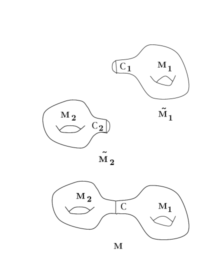
Figure 1: $M_{1},M_{2}$ are manifolds with boundary circles $C_{1},C_{2}$. They are capped off to form $\tilde{M}_{1},\tilde{M}_{2}$. They are sewn together to form the manifold $M$ without boundary

On the new manifold $M$ we have Gaussian fields $\{\phi(f):f\in H^{-1}(M)\}$ on a measure space $(Q,{\cal O},\mu)$. We also have an identification between fields on $M_{1}$ in $\tilde{M}_{1}$ and fields on $M_{1}$ in $M$. To see this first note that the isometry $j_{1}$ induces a map $j_{1,*}$ from distributions on $\tilde{M}_{1}$ with support in $M_{1}$ to distributions on $M$ with support in $M_{1}$. This map preserves Sobolev spaces and so

$$j_{1,*}:H^{-1}_{M_{1}}(\tilde{M}_{1})\to H^{-1}_{M_{1}}(M)$$ (34)

However with our nonlocal norms (4) this is not unitary. There is an induced map on Fock space subspaces:

$$J_{1}\equiv\Gamma(j_{1,*}):{\cal F}(H^{-1}_{M_{1}}(\tilde{M}_{1}))\to{\cal F}(H^{-1}_{M_{1}}(M))$$ (35)

Since $j_{1,*}$ is not a contraction $J_{1}$ is unbounded. We take as the domain elements with a finite number of entries. We can also regard $J_{1}$ as a map of the corresponding ${\cal L}^{2}$ subspaces

$$J_{1}:{\cal L}^{2}(Q_{1},{\cal O}_{1,M_{1}},d\mu_{1})\to{\cal L}^{2}(Q,{\cal O}_{M_{1}},d\mu)$$ (36)

with domain the polynomials. We note also that $J_{1}$ maps ${\cal H}_{C_{1}}$ to ${\cal H}_{C}\equiv{\cal L}^{2}(Q,{\cal O}_{C},d\mu)$. There is a similar map $J_{2}$.

Our goal is to sew together the operators $A_{C_{1},M_{1}}$ and $A_{C_{2},M_{2}}$ and obtain an managable functional integral on the new manifold $M$. The recipe is as follows. Starting with polynomials $F,G$ on $M_{1},M_{2}$ we propagate them to the circles $C_{1},C_{2}$ by forming $A_{C_{1},M_{1}}F$ and $A_{C_{2},M_{2}}G$. Then we map to the circle $C$ forming $J_{1}A_{C_{1},M_{1}}F$ and $J_{2}A_{C_{2},M_{2}}G$ in ${\cal H}_{C}$. Finally we take the inner product in ${\cal H}_{C}$. Thus we define

$$(A_{C_{1},M_{1}}F,\ A_{C_{2},M_{2}}G)=\int\overline{(J_{1}A_{C_{1},M_{1}}F)}(J_{2}A_{C_{2},M_{2}}G)d\mu$$ (37)

Theorem 3

(Sewing, $m>0$) Let $F$ be a polynomial in $\{\phi_{1}(f):f\in H_{M_{1}}^{-1}(\tilde{M}_{1})\}$ and let $G$ be a polynomial in $\{\phi_{2}(f):f\in H_{M_{2}}^{-1}(\tilde{M}_{2})\}$. Then

$$(A_{C_{1},M_{1}}F,\ A_{C_{2},M_{2}}G)=\int\overline{(J_{1}F)}(J_{2}G)d\mu$$ (38)

Remark. Thus sewing involves the identification operators $J_{1},J_{2}$ from $M_{1},M_{2}$ to $M$. These can be understood as a change in Wick ordering. We have

$$J_{1}\left(:\phi_{1}(f_{1})\dots\phi_{1}(f_{n}):_{(-\Delta_{\tilde{M}_{1}}+m^{2})^{-1}}\right)=:\phi(j_{1,*}f_{1})\dots\phi(j_{1,*}f_{n}):_{(-\Delta_{M}+m^{2})^{-1}}$$ (39)

Proof. We have that $j_{1,*}$ maps $H^{-1}_{M_{1}}(\tilde{M}_{1})$ to $H^{-1}_{M_{1}}(M)$. These spaces have the decompositions (13)

$$\begin{split}H^{-1}_{M_{1}}(\tilde{M}_{1})=&H^{-1}_{C_{1}}(\tilde{M}_{1})\oplus(-\Delta_{\tilde{M}_{1}}+m^{2})H_{0}^{1}(\textrm{int }M_{1})\\ H^{-1}_{M_{1}}(M)=&H^{-1}_{C}(M)\oplus(-\Delta_{M}+m^{2})H_{0}^{1}(\textrm{int }M_{1})\end{split}$$ (40)

and since $j_{1}$ is an isometry $j_{1,*}$ preserves the decomposition. The operators $e^{\tilde{M}_{1}}_{C_{1}}$ and $e^{M}_{C}$ are the projections onto the first factors and so we have the identity on $H^{-1}_{M_{1}}(\tilde{M}_{1})$

$$j_{1,*}\ e^{\tilde{M}_{1}}_{C_{1}}=e^{M}_{C}\ j_{1,*}$$ (41)

It follows that

$$J_{1}\ {\cal E}^{\tilde{M}_{1}}_{C_{1}}=\Gamma(j_{1,*})\Gamma(e^{\tilde{M}_{1}}_{C_{1}})=\Gamma(e^{M}_{C})\Gamma(j_{1,*})={\cal E}^{M}_{C}\ J_{1}$$ (42)

Then we have

$$\begin{split}(A_{C_{1},M_{1}}F,\ A_{C_{2},M_{2}}G)=&\int\overline{(J_{1}{\cal E}^{\tilde{M}_{1}}_{C_{1}}F)}(J_{2}{\cal E}^{\tilde{M}_{2}}_{C_{2}}G)d\mu\\ =&\int\overline{({\cal E}^{M}_{C}J_{1}F)}({\cal E}^{M}_{C}J_{2}G)d\mu\\ =&\int\overline{(J_{1}F)}(J_{2}G)d\mu\\ \end{split}$$ (43)

In the last step we use that $J_{1}F$ is ${\cal O}_{M_{1}}$ measurable, that $J_{2}G$ is ${\cal O}_{M_{2}}$ measurable, and the Markov property via the identity (21). This completes the proof.

Remarks.

(1.) We do not attempt a direct sewing result in the case $m=0$. However one can get something in this direction by restricting the class of test functions and taking the limit $m\to 0$ as in Corollary 3.

(2.) Our treatment has featured manifolds with a single boundary circle. However one could as well consider manifolds with many boundary circles $\{C_{i}\}$. In this case one would consider operators between (algebraic) tensor products of Hilbert spaces ${\cal H}_{C_{i}}$ based on the boundary circles. Again one can show a sewing property of the type we have presented. This is essentially the structure discussed by Segal [12] in his axioms for conformal field theory, except that we have not accommodated the possibility of sewing together boundary circles on the same manifold. See also Gawedski [4], Huang [6], and Langlands [8].

6 Interacting fields

We continue to restrict to $d=2$ and now study interacting fields on a compact Riemann surface $(M,g)$. For this we may as well assume $m>0$. We introduce a potential for $A\subset M$

$$V_{A}(\phi)=\int_{A}:P(\phi(x)):_{(-\Delta+m^{2})^{-1}}\sqrt{\det g(x)}dx$$ (44)

Here $P$ is a lower semi-bounded polynomial. This not obviously well-defined since it refers to products of distributions. However it turns out that the Wick ordering provides sufficient regularization and we have

Lemma 4

$V_{A},e^{-V_{A}}$ are functions in ${\cal L}^{p}(Q,{\cal O},d\mu)$ for all $p<\infty$.

In the plane and with $A$ compact this is a classic result of constructive field theory. [11], [13], [5]. The proof has been extended to compact subsets of paracompact complete Riemannian manifolds by De Angelis, de Falco, Di Genova [1]. Hence it holds for compact manifolds and an interacting field theory can be defined by the measure

$$d\nu=\frac{e^{-V_{M}}\ d\mu}{\int e^{-V_{M}}d\mu}$$ (45)

As noted by Gawedski [4] there may be special choices of the polynomial $P$ such that this is a conformal field theory.

For each measure $\nu$ we have the conditional expectation ${\cal E}_{A}^{\nu}F={\cal E}^{\nu}\{F|{\cal O}_{A}\}$. This conditional expectation can be expressed in terms of the conditional expectation ${\cal E}_{A}$ for $\mu$ by

$${\cal E}_{A}^{\nu}F=\frac{{\cal E}_{A}(Fe^{-V_{A^{c}}})}{{\cal E}_{A}(e^{-V_{A^{c}}})}$$ (46)

See [13] for this identity. Now the Markov property for $\nu$ follows directly from the Markov property for $\mu$. This is the following which generalizes the result of Nelson on the plane [11]:

Theorem 4

For open $\Omega\subset M$, let $F$ be ${\cal O}_{\bar{\Omega}}$ measurable. Then

$${\cal E}^{\nu}_{\Omega^{c}}F={\cal E}^{\nu}_{\partial\Omega}F$$ (47)

Acknowledgment: This work was initiated at the Institute for Advanced Study in Princeton whose hospitality I gratefully acknowledge.

References

[1] G. De Angelis, D. de Falco, G. Di Genova,
Random fields on Riemannian manifolds: a constructive approach.
Commun. Math. Phys. 103, 297-303, (1986)
[2] J. Dimock, models with variable coefficients,
Ann. of Phys. 154, 283-307, (1984).
[3] G. Felder, J. Frohlich, J. Keller, On the structure
of unitary conformal field theory, Commun. Math. Phys. 124, 417-463, (1989)
[4] K. Gawedski, Lectures on conformal field theory, in Quantum fields and strings: a course for
mathematicians, P. Deligne, et. al. ,eds, American Mathematical Society, Providence, 1999.
[5] J. Glimm, A. Jaffe, Quantum physics, an functional integral
point of view. Springer, New York, 1987.
[6] Y.Z. Huang, Two dimensional conformal geometry and vertex
operator algebras, Birkhauser, Boston, 1997.
[7] A. Jaffe, S.Klimek, A. Lesniewski,
Representations of the Heisenberg algebra on a Riemann
surface, Commun. Math. Phys. 126, 421-431, (1989)
[8] R.P. Langlands, The renormalization fixed point as
a mathematical object, IAS preprint.
[9] E. Nelson, Construction of quantum fields from Markov fields,
J. Func. Anal. 12, 97-112, (1973).
[10] E. Nelson, The free Markov field, J. Func. Anal. 12, 211-227, (1973).
[11] E. Nelson, Probability theory and Euclidean field
theory,
in G. Velo., A. Wightman, eds, Constructive Quantum field theory, Springer-Verlag,
New York, 1973.
[12] G. Segal, Two-dimensional conformal field theories and modular
functions, IX International Congress on Mathematical Physics, B. Simon, A. Truman,
and I.M. Davies, eds.,22-37, Adam Hilger, 1989.
[13] B. Simon, The Euclidean field theory, Princeton University Press,
Princeton, 1974.
[14] M. Taylor, Partial Differential Equations I, Springer, New York, 1996.