Geometric tools of the adiabatic complex WKB method

Abstract.

The paper is devoted to the description of the main geometric and analytic tools of a complex WKB method for adiabatic problem. We illustrate their use by numerous examples.

Résumé. L’article est consacré à la description des principaux outils géométriques et analytiques d’une méthode WKB complexe pour des problèmes adiabatiques. Nous illustrons leur utilisation par de nombreux exemples.

0. Introduction

In this paper, we study the asymptotic behavior of solutions of the one-dimensional Schrödinger equation

(0.1) $$-\frac{d^{2}\psi}{dx^{2}}\,(x)+V(x)\,\psi(x)+W(\varepsilon x)\,\psi(x)=E\,\psi(x),\quad x\in{\mathbb{R}},$$

where $\varepsilon$ is a small positive parameter, and $V(x)$ a real valued periodic function, $V(x+1)=V(x)$. We also assume that $V\in L^{2}_{loc}$ and that $\zeta\mapsto W(\zeta)$ is real analytic in some neighborhood of ${\mathbb{R}}\subset{\mathbb{C}}$.

The term $W(\varepsilon x)$ can be regarded as an adiabatic perturbation of the periodic potential $V(x)$. The analysis of perturbed periodic Schrödinger equations is a classical topic of mathematical physics. For example, in solid state physics, such equations models behavior of electrons in crystals placed in an external field ([2, 3]); in astrophysics, they model periodic motions perturbed by the presence of massive objects ([1]). As in solid state physics, so in astrophysics, the perturbations can often be regarded as very regular and slow varying with respect to the underlying periodic system. This naturally leads to an equation of the form (0.1).

0.1. Asymptotic methods

The classical WKB methods are used for the analysis of equations of the form

(0.2) $$-\frac{d^{2}\psi}{dx^{2}}+W(\varepsilon x)\psi(x)=E\psi(x).$$

The potential $W(\varepsilon\cdot)$ can be regarded as an adiabatic perturbation of the free operator $\displaystyle-\frac{d^{2}}{dx^{2}}$. In (0.1), $\displaystyle-\frac{d^{2}}{dx^{2}}$ is replaced by the periodic Schrödinger operator

(0.3) $$H_{0}=-\frac{d^{2}}{dx^{2}}(x)+V(x),\quad\quad V(x+1)=V(x),\quad x\in{\mathbb{R}}.$$

In [2], to study solutions of (0.1), V. Buslaev has suggested an analog the classical real WKB method. Both these methods do not allow to control important exponentially small effects (e.g. over barrier tunneling coefficients, exponentially small spectral gaps). To study these effect for (0.2), one can use the classical complex WKB method. And, in [8], we have developed an analog thereof to study such exponentially small effects for equation (0.1).

In our method (as in the classical complex WKB method), one assumes that the adiabatic perturbation $W(\cdot)$ is analytic and one tries to make the “slow” variable complex. But, in (0.1), as $V$ can be rather singular, one has to “decouple” the “slow” and the “fast” variables. We do this by introducing an additional parameter, say $\zeta$, so that equation (0.1) takes the form

(0.4) $$-\frac{d^{2}}{dx^{2}}\psi(x)+(V(x)+W(\varepsilon x+\zeta))\psi(x)=E\psi(x),\quad x\in{\mathbb{R}}.$$

The idea of our method is to study solutions of (0.4) on the complex plane of $\zeta$ and, then, to recover information on their behavior in $x$ along the real line.

There is a natural condition that can be imposed on solutions of (0.4) so as to relate their behavior in $x$ to their behavior in $\zeta$:

(0.5) $$\psi(x+1,\zeta)=\psi(x,\zeta+\varepsilon)\quad\forall\zeta.$$

We call it the consistency condition. On the complex plane of $\zeta$, there are certain canonical domains where the solutions satisfying the consistency condition have simple asymptotic behavior (see section 3.3 and Theorem 3.1):

(0.6) $$\psi(x,\zeta)=e^{\textstyle\frac{i}{\varepsilon}\int_{\zeta_{0}}^{\zeta}\kappa d\zeta}\left(\Psi(x,E-W(\zeta))+o(1)\right),\quad\varepsilon\to 0.$$

Here, $\Psi$ and $\kappa$ are a Bloch (Floquet) solution and the Bloch quasi-momentum (see sections 1.2 and 1.3) of the “unperturbed” periodic equation

(0.7) $$-\frac{d^{2}\Psi}{dx^{2}}+V(x)\Psi=\mathcal{E}\,\Psi,\quad\mathcal{E}=E-W(\zeta),\quad x\in{\mathbb{R}}.$$

Having constructed solutions having simple asymptotic behavior on a given canonical domain, one studies them outside this domain using the transfer matrix techniques as in the classical complex WKB method. The new asymptotic method has already been successfully applied to study spectral properties of quasi-periodic equations. In [10, 9, 6, 11], using this method, we have obtained a series of new results. However, trying to proceed as in the classical complex WKB method, one meets numerous technical problems which makes the computations very long. In this paper, we present a new geometric approach replacing or simplifying most of these computations.

0.2. Canonical domains

Canonical domains are defined in terms of $\kappa(\zeta)$, the complex momentum. This function satisfies

(0.8) $$\mathcal{E}(\kappa)+W(\zeta)=E,$$

where $\mathcal{E}$ is the dispersion law of the periodic operator (0.3). In the classical case, i.e. for $\displaystyle H_{0}=-\frac{d^{2}}{dx^{2}}$, relation (0.8) takes the form $\kappa^{2}+W(\zeta)=E$. The properties of the complex momentum in the adiabatic case are discussed in section 2.
Canonical domains are unions of canonical curves connecting two given points in ${\mathbb{C}}$ (“two points” condition). A canonical curve is roughly a smooth vertical curve (i.e. intersecting the lines ${\rm Im}\,\zeta=0$ at non-zero angles) along which the function ${\rm Im}\,\int^{\zeta}(\kappa-\pi)d\zeta$ decreases, and the function ${\rm Im}\,\int^{\zeta}\kappa d\zeta$ increases for increasing ${\rm Im}\,\zeta$ (see section 3.3 for the precise definition).
Recall that, in the classical case, in the definition of the canonical domains, there is no ”two points” condition, and the canonical lines are characterized by a growth condition on the function ${\rm Im}\,\int^{\zeta}\kappa d\zeta$. In our case, the “verticality” condition arises as the periodicity $V(x+1)=V(x)$ singles out the “horizontal” direction of the real line.
The basic fact of our method (established in [8]) is that, on any canonical domain, we can construct a solution with the standard behavior (0.6) (see Theorem 3.1). It is analytic in $\{Y_{1}<{\rm Im}\,\zeta<Y_{2}\}$, the smallest strip containing the canonical domain.

0.3. The new geometric approach and its strategy

When applying the classical complex WKB method, one first describes “maximal” canonical domains; then, to get the global asymptotics of a solution having simple asymptotic behavior on a given canonical domain, one expresses it in terms of the solutions having simple behavior on the other canonical domains. Therefore, one computes the “transfer” matrices relating basis of solutions having simple asymptotic behavior on different overlapping canonical domains.
In the case of adiabatic perturbations of the periodic Schrödinger operator, the definition of the canonical domains contains more conditions. In result, even “maximal” canonical domains are generally quite “small” in the ${\rm Re}\,\zeta$-direction. Moreover, “maximal” canonical domains become rather difficult to find. So, when computing the transfer matrices relating solutions with simple asymptotic behavior on two given different canonical domains, one has to consider a “long” chain of auxiliary overlapping canonical domains and to make many additional computations.
Fortunately, it appears that a solution having simple asymptotic behavior (0.6) on a canonical domain $K_{0}$ still has this behavior on domains which can be much larger than the maximal canonical domain containing $K_{0}$. Domains where a consistent solution $f$ has the simple asymptotic behavior (0.6) are called continuation diagrams of $f$. In this paper, we describe an elementary geometric approach to computing continuation diagrams.

Instead of trying to find “maximal” canonical domains, we begin by constructing a “thin” canonical domain. We use the following simple observation (see Lemma 4.1): any canonical line is contained in a local canonical domain “stretched” along the canonical line. To construct a canonical line, we use segments of some “elementary” curves described in section 4.1.2 (see also Proposition 4.1).
The main part of the work then consists in studying asymptotic behavior of the solution constructed with Theorem 3.1 outside the local canonical domain. It appears that there are three general principles allowing to compute the continuation diagram. We call these principles the main continuation tools.

So, to construct a solution with simple asymptotics on a large (not necessarily canonical) domain, we begin with a local canonical domain, and then, step by step, at each step applying one of the three continuation tools, we “extend” the continuation diagram, “continuing” (i.e. justifying) the simple asymptotics of $f$ to a larger domain.

0.4. The main continuation tools

There are three continuation tools: the Rectangle Lemma, Lemma 5.1, the Adjacent Canonical Domain Principle, Proposition 5.1 and the Stokes Lemma, Lemma 5.6. The first two principles were formulated and proved in [10] and [9]. The Stokes Lemma is proved in the present paper. We now briefly explain the respective roles of these tools and show how they complement one another when computing the continuation diagram.

The Rectangle Lemma. Roughly, the Rectangle Lemma says that a solution $f$ has the standard asymptotic behavior (0.6) along a horizontal line (i.e. a line ${\rm Im}\,\zeta={\rm Const}$) as long as the leading term of its asymptotics is growing along that line. This result is in agreement with the standard WKB heuristics saying that the asymptotics of a solution stays valid as long as its leading term is defined and increasing.

The leading term of the asymptotics contains the exponential factor $\exp(\textstyle\frac{i}{\varepsilon}\int^{\zeta}\kappa d\zeta)$. For small $\varepsilon$, this factor determines the size of the solution. If ${\rm Im}\,\kappa>0$ in some domain $D$, then, $f$ is increasing to the left; if ${\rm Im}\,\kappa<0$ in $D$, then, $f$ is increasing to the right. The Rectangle Lemma (Lemma 5.1) is formulated in terms of the sign of the imaginary part of $\kappa$.

Let $\gamma$ be the canonical line used to construct the solution $f$ locally. If, along a segment of $\gamma$,  ${\rm Im}\,\kappa>0$ (resp. ${\rm Im}\,\kappa<0$), then, $f$ keeps its simple behavior in a domain contiguous to $\gamma$ on its left (resp. right) side.

A natural obstacle for “continuation” by means of the Rectangle Lemma is a vertical line where ${\rm Im}\,\kappa=0$. So, usually, the domains where one justifies (0.6) by means of the Rectangle Lemma are curvilinear rectangles (or unions thereof).

The Adjacent Canonical Domain Principle. Let $\gamma_{0}$ be a curve canonical with respect to $\kappa_{0}$, some branch of the complex momentum. The Adjacent Canonical Domain Principle, Proposition 5.1, says that, if a solution $f$ has the simple behavior (0.6) in a domain adjacent to a canonical curve $\gamma_{0}$ then, $f$ keeps its simple behavior in any domain canonical with respect to $\kappa_{0}$ and enclosing $\gamma_{0}$.

The Adjacent Canonical Domain Principle is used to bypass the vertical curves which are obstacles for the use of the Rectangle Lemma. These can be either segments of the canonical line used to start the construction of $f$ or vertical lines along which ${\rm Im}\,\kappa=0$. In both cases, the obstacles are curves canonical with respect to some branch of the complex momentum.

By means of the Adjacent Canonical Domain Principle, one justifies the standard behavior in $A$, a domain the boundary of which contains the curve $\gamma_{0}$ and the lines beginning at the ends of $\gamma_{0}$ defined by equations of the form ${\rm Im}\,\int^{\zeta}\kappa_{0}d\zeta={\rm Const}$ and ${\rm Im}\,\int^{\zeta}(\kappa_{0}-\pi)d\zeta={\rm Const}$. Often these two lines intersect one another, and the domain $A$ has the shape of a curvilinear triangle. Otherwise, one considers domains $A$ of the form of a curvilinear trapezium; the fourth curve bounding such a trapezium is one more canonical curve. The precise description of these two possible situations is the subject of the Trapezium Lemma, Lemma 5.4.

The trapezium shaped domains are used to avoid the construction of “maximal” canonical domains enclosing $\gamma_{0}$ as this can be rather tricky. As the fourth boundary of the trapezium shaped domains, one usually chooses a curve which can be bypassed either by means of the other continuation tools or by applying The Adjacent Canonical Domain Principle once more.

The Stokes Lemma. Lemma 5.6 is akin to the results of the classical complex WKB method on the behavior of solutions in a neighborhood of a Stokes line where, instead of decreasing, they start to increase, see [5].
Consider $\zeta_{0}$ a branch point of the complex momentum. Assume $W^{\prime}(\zeta_{0})\neq 0$. As in the classical complex WKB method, such a point gives rise to three Stokes lines (i.e. lines starting at such a branch point defined by ${\rm Im}\,\int^{\zeta}(\kappa-\kappa(\zeta_{0}))d\zeta=0$).
Let $\sigma$ be one of these lines that moreover is vertical. Consider $V$, a neighborhood of $\sigma$ (more precisely, of a segment of $\sigma$ containing only one branch point, namely, $\zeta_{0}$). Assume that $V$ is so small that the Stokes lines divide it into three sectors (see Fig. 1). Let $S_{1}$ and $S_{3}$ be the sectors adjacent to $\sigma$, and let $S_{2}$ be the last sector. Roughly, the Stokes Lemma says that, if $f$ has the standard behavior inside $S_{1}\cup S_{2}$ and decreases as $\zeta\in S_{1}\cup S_{2}$ approaches $\sigma$ along the lines ${\rm Re}\,\zeta={\rm Const}$, then, $f$ has the standard behavior in $V\setminus\sigma$.
In result, to get the leading term of the asymptotics of $f$ in the sector $S_{3}$, one analytically continues this term from $S_{1}\cup S_{2}$ to $S_{3}$ inside $V\setminus\sigma$, i.e. around the branch point $\zeta_{0}$ avoiding the line $\sigma$.
The Stokes Lemma complements the Adjacent Canonical Domain Principle. Recall that the Adjacent Canonical Domain Principle allows to bypass vertical curves where ${\rm Im}\,\kappa=0$. The ends of the curves on which ${\rm Im}\,\kappa=0$ are branch points of the complex momentum. The Stokes lines beginning at these points usually form the upper and the lower boundaries of the domains where one justifies the standard behavior by means of the Adjacent Canonical Domain Principle. The Stokes Lemma, Lemma 5.6, allows us to justify the standard behavior beyond these lines by “going around” the branch points.

On the choice of the initial canonical line. For our construction to be successful, we have to make a suitable choice for the canonical line we start with. The idea is that this line should be close to the curve where the constructed solution is minimal: inside the continuation diagram, the factor $\left|\exp(\textstyle\frac{i}{\varepsilon}\int_{\zeta_{0}}^{\zeta}\kappa d\zeta)\right|$ has to increase as $\zeta$ moves away from this curve (along the lines ${\rm Im}\,\zeta={\rm Const}$). To achieve this, one builds the canonical line of segments of curves where ${\rm Im}\,\kappa=0$ and of segments of curves close to Stokes lines. In section 4.2, we construct a canonical line of such curves. In section, 6, we give a detailed example of the computation of a continuation diagram of a solution constructed on a canonical domain enclosing such a canonical line.

0.5. Two-Waves Principle

Recall that a continuation diagram is a domain where $f$, a given solution of (0.4) satisfying (0.5), has the simple behavior (0.6). In domains next to the continuation diagram, the leading term of the asymptotics of the solution is of the form

(0.9) $$A_{+}\,e^{\textstyle\frac{i}{\varepsilon}\int^{\zeta}\kappa d\zeta}\Psi_{+}(x,E-W(\zeta))+A_{-}\,e^{\textstyle-\frac{i}{\varepsilon}\int^{\zeta}\kappa d\zeta}\Psi_{-}(x,E-W(\zeta))$$

with coefficients $A_{\pm}$ that depend non trivially on $E$. This dependence makes it impossible to describe the solution by only one of the terms in (0.9) uniformly in $E$ and $\zeta$.
When studying a solution in domains adjacent to the continuation diagram one meets many different cases. In this paper, we discuss only one typical case. One encounters it when studying the solution in the domains “adjacent” to the local canonical domain where the construction of the solution was started. The precise geometrical situation is described in section 7; the behavior of the solution is governed by the Two-Waves Principle, Lemma 7.1, see also comments in section 7.3.

Note that, in the case of the Two-Waves Principle, one of the coefficients $A_{\pm}$ rapidly oscillates as a function of $E$ (for $\varepsilon\to 0$) and “periodically” vanishes. Its zeros are described by a Bohr-Sommerfeld like condition. Recall that, when starting, we try to construct solutions along the lines where they are minimal. The values of $E$ for which one of the coefficients in (0.9) vanishes can be regarded as some sort of “resonances”; when $E$ takes a “resonant” value, the solution becomes minimal along a new curve.

0.6. Examples

In all the examples we have treated so far ([9, 6, 11, 7]), we have seen that, for a suitable choice for the initial canonical line, the continuation diagram of the solution can be effectively computed by means of the continuation tools described above. In the present paper, instead of trying to formulate and prove this observation as a general statement, we illustrate all our constructions by detailed examples. In these examples, we assume that $W(\zeta)=\alpha\cos\zeta$, that all the gaps of the periodic operator (0.3) are open, and that the energy $E$ satisfies

(C):

$[E_{2n}-\delta,E_{2n+1}+\delta]\subset[E-\alpha,E+\alpha]\subset(E_{2n-1},E_{2n+2})$,

where $[E_{2n-1},E_{2n}]$ and $[E_{2n+1},E_{2n+2}]$ are two neighboring spectral bands of the periodic operator (0.3). This case is of special interest in the sense that it will illustrate the use of all our tools. From the quantum physicist’s point of view, this is the case when $[E_{2n-1},E_{2n}]$ and $[E_{2n+1},E_{2n+2}]$, the spectral bands of $H_{0}$, interact due “through” the adiabatic perturbation. In this case, one can observe several new interesting spectral phenomena, see [7, 11]. The examples we consider in the present paper are used to study these effects (see [7]).

0.7. The structure of the paper

In this text, we describe general constructions and results step by step, illustrating each step with examples. More or less long proofs of general results are postponed until the end of the paper.

Throughout the paper, we shall use a number of well known facts on the periodic Schrödinger operator (0.3). They are described in section 1. In subsection 1.4, we also introduce an analytic object defined in terms of the periodic operator; it is playing an important role for the adiabatic constructions.
In section 2, we define and study the complex momentum and related objects (e.g. Stokes lines). We complete this section (subsection 2.4) with the analysis of the complex momentum and the Stokes line for $W(\zeta)=\alpha\cos\zeta$.
In section 3, we introduce the concept of standard behavior and define canonical lines and canonical domains; we also formulate Theorem 3.1 on the solutions having standard behavior on a given canonical domain.
In section 4, we define local canonical domains and explain how to build canonical lines from segments of “elementary curves”. Having presented general results, in subsection 4.2, as an example, we construct a canonical line using this method.
Section 5 is devoted to the main continuation principles and related objects. The Trapezium Lemma, Lemma 5.4, is proved in section 8. The Stokes Lemma, Lemma 5.6, is proved in section 9.
In section 6, we give a detailed example of the computation of a continuation diagram.
Section 7 is devoted to the Two-Waves Principle. In subsection 7.4, on a detailed example, we show how to use it. The proof of the Two-Waves principle can be found in section 10.

1. Periodic Schrödinger operators

We first formulate well known results used throughout the paper. Their proofs can be found, for example, in [4, 12, 13, 14]. In the end of the section, we discuss a meromorphic function constructed in terms of the periodic operator. This function plays an important role for the adiabatic constructions.
Recall that the potential $V$ in (0.3) is assumed to be a $1$-periodic, real valued, $L^{2}_{loc}$-function.

1.1. Gaps and bands

The spectrum of the periodic operator (0.3) is absolutely continuous and consists of intervals of the real axis $[E_{1},\,E_{2}]$, $[E_{3},\,E_{4}]$, $\dots$, $[E_{2n+1},\,E_{2n+2}]$, $\dots$, such that

$$E_{1}<E_{2}\leq E_{3}<E_{4}\dots E_{2n}\leq E_{2n+1}<E_{2n+2}\leq\dots\,,$$

$$E_{n}\to+\infty,\quad n\to+\infty.$$

The points $E_{j}$,  $j=1,2,3\dots$, are the eigenvalues of the differential operator (0.3) acting on $L^{2}([0,2])$ with periodic boundary conditions. The intervals defined above are called the spectral bands, and the intervals $(E_{2},\,E_{3})$, $(E_{4},\,E_{5})$, $\dots$, $(E_{2n},\,E_{2n+1})$, $\dots$, are called the spectral gaps. If $E_{2n}<E_{2n+1}$, we say that the $n$-th gap is open.

1.2. Bloch solutions

Let $\psi$ be a solution of the equation

(1.1) $$-\frac{d^{2}}{dx^{2}}\psi\,(x)+V\,(x)\psi\,(x)=E\psi\,(x),\quad x\in{\mathbb{R}},$$

satisfying the relation $\psi\,(x+1)=\lambda\,\psi\,(x)$ for all $x\in{\mathbb{R}}$ with $\lambda\in{\mathbb{C}}$ independent of $x$. Such a solution is called a Bloch solution, and the number $\lambda$ is the Floquet multiplier. Let us discuss the analytic properties of Bloch solutions as functions of the spectral parameter.

Consider $\mathcal{S}_{\pm}$, two copies of the complex plane of energies cut along the spectral bands. Paste them together to get a Riemann surface with square root branch points. We denote this surface by $\mathcal{S}$.
There exists a Bloch solution $E\mapsto\psi(x,E)$ of equation (1.1) meromorphic on $\mathcal{S}$. We normalize it by the condition $\psi(0,E)\equiv 1$. The poles of this solution are located in the spectral gaps. More precisely, for each spectral gap, there is one and only one pole projecting into this gap. This pole is located either on $\mathcal{S}_{+}$ or on $\mathcal{S}_{-}$. The position of the pole is independent of $x$.

Except at the edges of the spectrum (i.e. the branch points of $\mathcal{S}$), the two branches of $\psi$ are linearly independent solutions of (1.1).

Finally, we note that, in the spectral gaps, both branches of $\psi$ are real valued functions of $x$, and, on the spectral bands, they differ only by complex conjugation.

1.3. The Bloch quasi-momentum

Consider the Bloch solution $\psi(x,E)$. The corresponding Floquet multiplier $\lambda\,(E)$ is analytic on $\mathcal{S}$. Represent it in the form $\lambda(E)=\exp(ik(E))$. The function $k(E)$ is the Bloch quasi-momentum.

The Bloch quasi-momentum is an analytic multi-valued function of $E$. It has the same branch points as $\psi(x,E)$.
Let $D$ be a simply connected domain containing no branch point of the Bloch quasi-momentum. In $D$, one can fix an analytic single-valued branch of $k$, say $k_{0}$. All the other single-valued branches of $k$ that are analytic in $E\in D$ are related to $k_{0}$ by the formulae

(1.2) $$k_{\pm,l}(E)=\pm k_{0}(E)+2\pi l,\quad l\in{\mathbb{Z}}.$$

Consider ${\mathbb{C}}_{+}$ the upper half of the complex plane. On ${\mathbb{C}}_{+}$, one can fix a single valued analytic branch of the quasi-momentum continuous up to the real line. We can and do fix it by the condition $-ik(E+i0)>0$ for $E<E_{1}$. We call this branch the main branch of the Bloch quasi-momentum and denote it by $k_{p}$.
The function $k_{p}$ conformally maps ${\mathbb{C}}_{+}$ onto the first quadrant of the complex plane cut at compact vertical slits beginning at the points $\pi l$, $l\in{\mathbb{N}}$. It is monotonically increasing along the spectral bands so that $[E_{2n-1},E_{2n}]$, the $n$-th spectral band, is mapped on the interval $[\pi(n-1),\pi n]$. Inside any open gap, ${\rm Re}\,k_{p}(E)$ is constant, and ${\rm Im}\,k_{p}(E)$ is positive and has only one non-degenerate maximum. If the $n$th gap is open, in this gap, one has ${\rm Re}\,k_{p}(E)=\pi n$.
All the branch point of $k_{p}$ are of square root type: let $E_{l}$ be a branch point; then, in a sufficiently small neighborhood of $E_{l}$, the function $k_{p}$ is analytic in $\sqrt{E-E_{l}}$, and

(1.3) $$k_{p}(E)-k_{p}(E_{l})=c_{l}\sqrt{E-E_{l}}+O(E-E_{l}),\quad c_{l}\not=0.$$

Finally, we note that the main branch can be analytically continued on the complex plane cut only along the spectral gaps of the periodic operator.

1.4. A meromorphic function $\mathbf{\omega}$ and the differential $\mathbf{\Omega}$

We now define a meromorphic function on $\mathcal{S}$, the Riemann surface associated to the periodic operator (0.3). First, we have to recall more facts and to introduce some notations.

1.4.1. Periodic component of the Bloch solution

At a given energy $E$, the Bloch solution $\psi(x,E)$ can be represented in the form

(1.4) $$\psi(x,E)=e^{\textstyle ik(E)x}p(x,E),$$

where $k(E)$ is the Bloch quasi-momentum of $\psi(x,E)$ at $E$, and the function $p(x,E)$ is $1$-periodic in $x$. The function $p$ is called the periodic component of $\psi$ with respect to the branch $k(E)$.
Note that, as $k(E)$ is defined modulo $2\pi$, the function $p(x,E)$ is defined up to the factor $e^{2\pi imx}$, $m\in{\mathbb{Z}}$. The branches $p$ and $k$ are related by

(1.5) $$k\to k+2\pi m\quad\Longleftrightarrow p\to e^{-2\pi imx}\,p.$$

1.4.2. Notations

For $E\in\mathcal{S}$, let $\hat{E}$ be the other point in $\mathcal{S}$ having the same projection on ${\mathbb{C}}$ as $E$. We let

(1.6) $$\hat{\psi}(x,E)=\psi(x,\hat{E}),\quad\hat{k}(E)=-k(E),\quad\hat{p}(x,E)=e^{-\textstyle i\hat{k}(E)\,x}\,\hat{\psi}(x,E).$$

The function $\hat{\psi}$ is one more Bloch solution of the periodic Schrödinger equation that, for $E$ outside $\{E_{l}\}$, is linearly independent of $\psi(x,E)$. The function $\hat{k}$ is its quasi-momentum, and $\hat{p}$ its periodic component.

1.4.3. The sets $P$ and $Q$

Introduce two discrete sets on $\mathcal{S}$. Let $P$ be the set of poles of the Bloch solution $\psi(x,E)$, and, $Q$ be the set of the points where $k^{\prime}(E)=0$.
Recall that the points of $Q$ are (projected) inside open gaps of the periodic operator (one point per gap), and that the points of $P$ are (projected) either inside open gaps or at their edges (also one point per open gap).

1.4.4. Local construction of the function $\omega$ and the differential $\Omega$

Let $D\subset\mathcal{S}\setminus\{E_{l}\}$ be a simply connected domain. On $D$, fix $k$, an analytic branch of the Bloch quasi-momentum of $\psi$. Then, the functions $p$ and $\hat{p}$ are meromorphic on $D$. We let

(1.7) $$\omega(E)=-\frac{\int_{0}^{1}\hat{p}(x,\,E)\,\frac{\partial p}{\partial E}(x,\,E)dx}{\int_{0}^{1}p(x,\,E)\,\hat{p}(x,\,E)dx},\quad\text{and}\quad\Omega(E)=\omega(E)\,dE.$$

Note that the function $\omega$ was introduced and analyzed in the paper [9]. Using the differential $\Omega$ instead of this function makes computations more transparent. We have

Lemma 1.1.

$\Omega$ is a meromorphic differential on $D$. All its poles are simple; they are situated at exactly the points of $P\cup Q$. The residues are given by the formulae:

(1.8) $${\rm res}\,_{p}\Omega=1,\quad\forall p\in P\setminus Q,\quad\quad{\rm res}\,_{q}\Omega=-1/2,\quad\forall q\in Q\setminus P,\quad\quad{\rm res}\,_{r}\Omega=1/2,\quad\forall r\in Q\cap P.$$

Lemma 1.1 follows from the analysis made in [9] when proving Lemma 3.1. We omit the details.

1.4.5. Global properties of $\Omega$

By means of (1.5), we see that, $\omega$ and $\Omega$ do not depend on the choice of the branch $k$. Hence, $\omega$ and $\Omega$ are uniquely defined on $\mathcal{S}\setminus\{E_{l}\}$. One can analyze $\Omega$ on the whole Riemann surface $\mathcal{S}$ ($\infty$ was not “included” in $\mathcal{S}$). This gives

Lemma 1.2.

$\Omega$ is a meromorphic differential on the whole Riemann surface $\mathcal{S}$. Its poles and the residues at these poles are described in Lemma 1.1.

Proof.  In view of Lemma 1.1, it suffices to study $\Omega$ in $V_{n}$, a sufficiently small neighborhood of $E_{n}$, an end of a spectral gap. Recall that $k^{\prime}$ has zeros only inside open gaps. So, as $V_{n}$ can be taken arbitrarily small, there are two cases to consider:

• either $P\cap V_{n}=\emptyset$,

• or $E_{n}\in P$.

We have to show that $\Omega$ is holomorphic in $V_{n}$ with respect to the local variable $\tau=\sqrt{E-E_{n}}$. Consider the first case. Recall that $k$ is analytic (holomorphic) in $\tau$. So, $p$ and $\hat{p}$ are also holomorphic in $\tau$, and we have only to check that the function $f(\tau)=\int_{0}^{1}p\,\hat{p}\,dx=\int_{0}^{1}\psi\,\hat{\psi}\,dx$ does not vanish at $\tau=0$. At the end of any spectral gap, one has $\hat{\psi}=\psi$, and $\psi$ is real. So, $f(0)=\int_{0}^{1}|\psi(x,E_{n})|^{2}dx>0$. This completes the proof in the first case.
In the second case, one has to prove that $\Omega$ has a simple pole at $\tau=0$, and that ${\rm res}\,_{\tau=0}\Omega=1$. Now, in $V_{n}$, $\psi(x,\tau)=\psi_{0}(x)/\tau+({\rm\ a\ holomorphic\ function})$. The function $\psi_{0}$ is a (non-trivial) Bloch solution of (0.7) at $E=E_{n}$. It is real valued. This and the definitions of $p$ and $\hat{p}$ imply that, in $V_{n}$, one has $\Omega=d\tau/\tau+({\rm\ a\ holomorphic\ differential})$. This completes the analysis of the second case and, therefore, the proof of Lemma 1.2.∎

1.4.6. Differential $\Omega$ and analytic Bloch solutions

Let us formulate a very important property of $\Omega$. Consider again a simply connected domain $D\subset\mathcal{S}$. Pick $E_{0}\in D\setminus(P\cup Q)$. In a sufficiently small neighborhood of $E_{0}$, one can define the function

(1.9) $$\sqrt{k_{E}^{\prime}(E)}\,\,e^{\textstyle\int_{E_{0}}^{E}\Omega}\,\psi(x,\,E).$$

It is also a Bloch solution of the periodic Schrödinger equation. Lemma 1.2 immediately implies that it can be analytically continued on the whole domain $D$.

1.4.7. The function $\omega$ along gaps and bands

In applications, one uses the following observations:

Lemma 1.3.

Along open gaps, the values of $\omega$ are real. Along bands, $\omega(E)$ and $\omega(\hat{E})$ only differ by complex conjugation.

Proof.  The statements follow from the facts that, along the gaps, $\psi$ is real and $k$ is purely imaginary modulo $2\pi$, and that along the bands, $\psi$ and $\hat{\psi}$ differ by complex conjugation, and $k$ is real.∎

2. The complex momentum

The main analytic object of the complex WKB method is the complex momentum. We now define and discuss it as well as some related objects (e.g. the Stokes lines). We complete this section with an example: we discuss the complex momentum and the Stokes lines for $W(\zeta)=\alpha\cos\zeta$.

2.1. Definition and elementary properties

Definition 2.1.

For $\zeta\in{\mathcal{D}}(W)$, the domain of analyticity of the function $W$, the complex momentum is defined by

(2.1) $$\kappa(\zeta)=k(E-W(\zeta))$$

where $k$ is the Bloch quasi-momentum of (0.3).

Clearly, the complex momentum can also be interpreted the Bloch quasi-momentum for the periodic Schrödinger equation (0.7) regarded as a function of the complex parameter $\zeta$.

2.1.1. Branch points

The relation between $k$ and $\kappa$ shows that the complex momentum is a multi-valued analytic function, and that its branch points are related to the branch points of the quasi-momentum by the relations

(2.2) $$E_{j}=E-W\,(\zeta),\quad j=1,2,3,\,\dots$$

Note that all of them are situated on $W^{-1}({\mathbb{R}})$, the pre-image of the real line with respect to $W$.

Let $\zeta_{0}$ be a branch point of $\kappa$. Assume $W^{\prime}(\zeta_{0})\neq 0$. Then, this branch point is of square root type: in a neighborhood of $\zeta_{0}$, $\kappa$ is analytic in $\sqrt{\zeta-\zeta_{0}}$, and

(2.3) $$\kappa(\zeta)-\kappa(\zeta_{0})\sim\kappa_{1}\sqrt{\zeta-\zeta_{0}},\quad\kappa_{1}\neq 0.$$

2.1.2. Regular domains and branches of the complex momentum

Definition 2.2.

We say that a set is regular if it is a simply connected subset of the domain of analyticity of $W$ that contains no branch points of $\kappa$.

Let $D$ be a regular domain. In $D$, one can fix an analytic branch of $\kappa$, say $\kappa_{0}$. By (1.2), all the other branches of $\kappa$ analytic on $D$ are described by the formulas

(2.4) $$\kappa_{m}^{\pm}=\pm\kappa_{0}+2\pi m,$$

where $\pm$ and $m$ are indexing the branches.

Fix a branch point $\zeta_{0}$ such that $W^{\prime}(\zeta_{0})\neq 0$ and, let $V$ be a neighborhood of $\zeta_{0}$. Let $c$ be a smooth curve beginning at $\zeta_{0}$ and such that $V\setminus c$ is a regular domain. In $V\setminus c$, fix an analytic branch of the complex momentum. Then, by (2.3), $\kappa_{1}(\zeta)$ and $\kappa_{2}(\zeta)$, the values of this branch in $V$ on the different sides of $c$, are related by the formula

(2.5) $$\kappa_{1}(\zeta)+\kappa_{2}(\zeta)=2\kappa(\zeta_{0}),\quad\zeta\in c.$$

2.2. Stokes lines and lines of Stokes type

In the constructions of the complex WKB method, integrals of the form $\int^{\zeta}\kappa\,d\zeta$ and $\int^{\zeta}(\kappa-\pi)\,d\zeta$ play an important role. Their properties are described in terms of lines of Stokes type and Stokes lines.

2.2.1. Lines of Stokes type

Let $D$ be a regular domain. On $D$, fix an analytic branch of the complex momentum. Pick $\zeta_{0}\in D$.

Definition 2.3.

The level curves of the harmonic functions ${\rm Im}\,\int_{\zeta_{0}}^{\zeta}\kappa\,d\zeta$ and ${\rm Im}\,\int_{\zeta_{0}}^{\zeta}(\kappa-\pi)\,d\zeta$ are called lines of Stokes type.

Clearly, lines of Stokes type do not depend on the choice of $\zeta_{0}$.

To analyze the geometry of the lines of Stokes type, one uses the following lemma (where we identify the complex numbers with vectors in ${\mathbb{R}}^{2}$). One has

Lemma 2.1.

The lines of the family ${\rm Im}\,\int^{\zeta}\kappa\,d\zeta={\rm Const}$ are tangent to the vector field $\overline{\kappa(\zeta)}$; the lines of the family ${\rm Im}\,\int^{\zeta}(\kappa-\pi)\,d\zeta={\rm Const}$ are tangent to the vector field $\overline{\kappa(\zeta)}-\pi$.

This lemma implies that the lines of Stokes type are trajectories of the differential equations $\displaystyle\frac{d\zeta}{dt}=\overline{\kappa(\zeta)}$ and $\displaystyle\frac{d\zeta}{dt}=\overline{\kappa(\zeta)}-\pi$. So, to study properties of the lines of Stokes type, one can use standard facts from the theory of differential equations. In particular, we get

Corollary 2.1.

The lines of Stokes type of each of the two families fibrate any regular domain $D$.

Proof.  For sake of definiteness, consider the lines of the family ${\rm Im}\,\int^{\zeta}\kappa\,d\zeta={\rm Const}$. It suffices to show that the vector field $\overline{\kappa(\zeta)}$ does not vanish in $D$. But, we know, that $\kappa$ takes values in $\pi{\mathbb{Z}}$ only at branch points of the complex momentum. As $D$ is regular, it does not contain any of these points. This completes the proof of Corollary 2.1. ∎

2.3. Stokes lines

Below, we always work in the domain of analyticity of $W$. Let $\zeta_{0}$ be a branch point of the complex momentum. A Stokes line beginning at $\zeta_{0}$ is a curve $\gamma$ defined by the equation $\text{Im}\,\int_{\zeta_{0}}^{\zeta}(\kappa\,(\xi)-\kappa\,(\zeta_{0}))d\zeta=0$. Here, $\kappa$ is a branch of the complex momentum continuous on $\gamma$.
It follows from (2.4) that the Stokes lines starting at $\zeta_{0}$ are independent of the choice of the branch of $\kappa$ in the definition of a Stokes line.
Assume that $W^{\prime}(\zeta_{0})\neq 0$. Then, in a neighborhood of the branch point $\zeta_{0}$, one has (2.3). Hence, there are three Stokes lines beginning at $\zeta_{0}$. At the branch point, the angle between any two of them is equal to $2\pi/3$.

Figure 1. The Stokes lines in a neighborhood of a branch point

One can always choose a branch of the complex momentum (see (2.4)) continuous on a given Stokes line $\gamma$ and such that either $\kappa(\zeta_{0})=0$ or $\kappa(\zeta_{0})=\pi$. We call this branch natural. With respect to the natural branch, the Stokes lines are lines of Stokes type.
Consider $V$, a neighborhood of $\zeta_{0}$. If $V$ is sufficiently small, the Stokes lines beginning at $\zeta_{0}$ divide $V$ into three domains called sectors, see Fig. 1.
Let $\kappa(\zeta_{0})=0$ (resp. $\kappa(\zeta_{0})=\pi$). Then, each of the sectors is fibrated by the lines of Stokes type of the family ${\rm Im}\,\int^{\zeta}\kappa d\zeta=Const$ (resp. ${\rm Im}\,\int^{\zeta}(\kappa-\pi)d\zeta=Const$). In particular, the part of the boundary of such a sector formed by two Stokes lines can be approximated arbitrarily well by a line of Stokes type ${\rm Im}\,\int^{\zeta}\kappa d\zeta=Const$ (resp. ${\rm Im}\,\int^{\zeta}(\kappa-\pi)d\zeta=Const$) intersecting this sector, see Fig. 1.

2.4. Example: complex momentum and Stokes lines for $\mathbf{W(\zeta)=\alpha\cos\zeta}$

We now discuss the complex momentum and describe the Stokes lines when $W(\zeta)=\alpha\cos\zeta$. We assume that all the gaps of the periodic operator (0.3) are open, and that the spectral parameter $E$ satisfies condition (C).

2.4.1. Complex momentum

1.  The set of branch points is $2\pi$-periodic and symmetric with respect both to the real line and to the imaginary axis. For $E$ real, the branch points of the complex momentum are situated on the lines of the set $W^{-1}({\mathbb{R}})$. For $W(\zeta)=\alpha\cos\zeta$, this set consists of the real line and the lines ${\rm Re}\,\zeta=\pi l$, $l\in{\mathbb{Z}}$.

Define the half-strip

Figure 2. $(z_{l})_{l}$ and $(g_{l})_{l}$

(2.6) $$\hskip-113.81102pt\Pi=\{\zeta\in{\mathbb{C}}:\ 0<{\rm Re}\,\zeta<\pi,\ {\rm Im}\,\zeta>0\}.$$

This half-strip is a regular domain. Consider the branch points situated on $\partial\Pi$, the boundary of $\Pi$. $\partial\Pi$ is bijectively mapped by $\mathcal{E}:\zeta\to E-W(\zeta)$ onto the real line. So, for any $j\in{\mathbb{N}}$, there is exactly one branch point described by (2.2). We denote this point by $\zeta_{j}$. Under condition (C), the branch points $\zeta_{2n}$ and $\zeta_{2n+1}$ are situated on the interval $(0,\pi)$, i.e.

$$\hskip-113.81102pt0<\zeta_{2n}<\zeta_{2n+1}<\pi;$$

the branch points $\zeta_{1}$, $\zeta_{2}$, $\dots$ $\zeta_{2n-1}$ are situated on the imaginary axis so that

$$\hskip-113.81102pt0<{\rm Im}\,\zeta_{2n-1}<\dots<{\rm Im}\,\zeta_{2}<{\rm Im}\,\zeta_{1};$$

the other branch points are situated on the line ${\rm Re}\,\zeta=\pi$ so that

$$0<{\rm Im}\,\zeta_{2n+2}<{\rm Im}\,\zeta_{2n+3}<\dots$$

In Fig. 2, we show some of the branch points. 2.  The half-strip $\Pi$ is mapped by $\mathcal{E}:\zeta\to E-\alpha\cos\zeta$ on the upper half of the complex plane. So, on $\Pi$, we can define a branch of the complex momentum by the formula

(2.7) $$\hskip-113.81102pt\kappa_{p}(\varphi)=k_{p}(E-\alpha\cos\varphi),$$

$k_{p}$ being the main branch of the Bloch quasi-momentum for the periodic operator (0.3). We call $\kappa_{p}$ the main branch of the complex momentum.

The main branch of the Bloch quasi-momentum was discussed in details in section 1.3. The properties of $k_{p}$ are “translated” into properties of $\kappa_{p}$ using formula (2.7). In particular, $\kappa_{p}$ conformally maps $\Pi$ into ${\mathbb{C}}_{+}$. Fix $l$, a positive integer. The closed segment $z_{l}:=[\zeta_{2l-1},\zeta_{2l}]\subset\partial\Pi$ is bijectively mapped on the interval $[\pi(l-1),\pi l]$, and, on the open segment $g_{l}:=(\zeta_{2l},\zeta_{2l+1})\subset\partial\Pi$, the real part of $\kappa$ equals to $\pi l$, and its imaginary part is positive. The intervals $(z_{l})_{l}$ and $(g_{l})_{l}$ are shown in Fig. 2.

2.4.2. Stokes lines

Let us discuss the set of Stokes lines for $W(\zeta)=\alpha\cos\zeta$. Due to the symmetry properties of $\mathcal{E}$, the set of the Stokes lines is $2\pi$-periodic and symmetric with respect to both the real and imaginary axes.

In Fig. 3, we have represented Stokes lines in $\Pi$ by dashed lines. Consider the Stokes lines beginning at the branch points $\zeta_{l}$ with $l\geq 2n$. The other Stokes lines beginning at points of $\partial\Pi$ are analyzed similarly. We begin with properties following immediately from the definition of Stokes lines.

Elementary properties of Stokes lines. Consider the Stokes lines beginning at $\zeta_{2n+1}$. The interval $[\zeta_{2n+1},\pi]$ is a part of $z_{n+1}$. So, $\kappa_{p}$ is real on this interval, and, therefore, this interval is a part of a Stokes line beginning at $\zeta_{2n+1}$. The two other Stokes lines beginning at $\zeta_{2n+1}$ are symmetric with respect to the real line, see Fig. 3. We denote by “a” the Stokes line going upward from $\zeta_{2n+1}$.

Consider the Stokes lines beginning at $\zeta_{2n+2}$. As $\kappa_{p}(\zeta_{2n+2})=\pi(n+1)$, they satisfy ${\rm Im}\,\int_{\zeta_{2n+2}}^{\zeta}(\kappa_{p}(\zeta)-\pi(n+1))d\zeta=0$. Recall that, along the segment $g_{n+1}=(\zeta_{2n+2},\zeta_{2n+3})$ of the line ${\rm Re}\,\zeta=\pi$, one has ${\rm Re}\,\kappa_{p}=\pi(n+1)$. So, this segment is a Stokes line beginning at $\zeta_{2n+2}$. The two other Stokes lines beginning at $\zeta_{2n+2}$ are symmetric with respect to the line ${\rm Re}\,\zeta=\pi$, see Fig. 3. We denote by “b” the Stokes line going to the left from $\zeta_{2n+2}$. The Stokes lines beginning at other branch points situated on the right part of $\partial\Pi$ are analyzed similarly to the ones beginning at $\zeta_{2n+2}$.

Global properties of “a”, …, “d” and “e”. These Stokes lines shown in Fig. 3 are described by

Lemma 2.2.

The Stokes lines “a”,…, “d” and “e” have the following properties:

Figure 3. The Stokes lines

• the Stokes lines “a” and “e” stay inside $\Pi$, are vertical and do not intersect one another;

• the Stokes line “c” stays between “a” and the line ${\rm Re}\,\zeta=\pi$ (without intersecting them) and is vertical;

• before leaving $\Pi$, the Stokes lines “b” stays vertical, and it intersects “a” first at a point with positive imaginary part;

• before leaving $\Pi$, the Stokes lines “d” stays vertical and intersects “c” first above $\zeta_{2n+3}$, the beginning of “c”.

Proof.  The main tool in the proof is Lemma 2.1. Below, we use it without referring to it.
First, we note that, as ${\rm Im}\,\kappa\neq 0$ in $\Pi$, the Stokes lines “a”, “b”,…, “e” stay vertical as long as they stay in $\Pi$.
Second, one checks that the Stokes lines “a”,…, “d” cannot leave $\Pi$ by intersecting the line ${\rm Re}\,\zeta=\pi$ (the right boundary of $\Pi$), and that “e” cannot leave $\Pi$ by intersecting the imaginary axis (the left boundary of $\Pi$). We check this property for “a” only; the analysis of the other lines is similar. Note that “a” is tangent to the vector field $\overline{\kappa(\zeta)}-\pi n$. Consider this vector field in a sufficiently small neighborhood of the line ${\rm Re}\,\zeta=\pi$ (in $\Pi$). There, we have ${\rm Re}\,\kappa>\pi n$ and ${\rm Im}\,\kappa>0$. Therefore, “a” can intersect the line ${\rm Re}\,\zeta=\pi$ only when coming from above to the right. But, this is impossible as “a” begins at $\zeta_{2n+1}$ and stays vertical while in $\Pi$.
To prove the first point of Lemma 2.2, it suffices to check that “a” and “e” do not intersect one another while in $\Pi$. Therefore, we note that both lines belong to the family ${\rm Im}\,\int^{\zeta}(\kappa-\pi n)d\zeta={\rm Const}$. Therefore, by Lemma 2.1, while in $\Pi$, “a” and “e” either stay disjoint or coincide. The second is impossible as they begin at distinct points of the real line, and, inside $\Pi$, each of them is smooth and vertical.
To prove the second point of Lemma 2.2, it suffices to check that “a” and “c” do not intersect one another while in $\Pi$. Therefore, we note that “a” is tangent to the vector field $v_{1}(\zeta)=\overline{\kappa(\zeta)}-\pi n$, and that “c” is tangent to the vector field $v_{2}(\zeta)=\overline{\kappa(\zeta)}-\pi(n+1)$. Pick $\zeta_{0}\in\Pi$. As ${\rm Im}\,\kappa(\zeta_{0})>0$, both vectors $v_{1}(\zeta_{0})$ and $v_{2}(\zeta_{0})$ are oriented downward, and $v_{1}$ is oriented to the right of $v_{2}$. So, to intersect “a”, the line “c” has to approach it going from left to right. But, this is impossible as “c” begins to the right of “a”.
To prove the third point of Lemma 2.2, it suffices to check that “b” can not leave $\Pi$ intersecting the segment $[\zeta_{2n+1},\pi]$ of the real line. Therefore, we note that both this segment and “b” belong to the family of lines ${\rm Im}\,\int^{\zeta}(\kappa-\pi(n+1))d\zeta={\rm Const}$. So, by Lemma 2.1, “b” cannot intersect the segment $(\zeta_{2n+1},\pi]$. Finally, a local analysis using the Implicit Function Theorem shows that “b” can not contain the point $\zeta_{2n+1}$.
The last point of Lemma 2.2 follows from the second one as we have seen that, in $\Pi$, “d” goes downwards from $\zeta_{2n+3}$ and stays vertical; moreover, it cannot leave $\Pi$ intersecting $\Pi$’s right boundary.
This completes the proof of Lemma 2.2 ∎

The analysis of the other Stokes lines situated inside $\Pi$ is analogous to the one made in the proof of Lemma 2.2.

3. Standard behavior of solutions

Here, we introduce the concept of the standard behavior of solutions of (0.4) studied in the framework of the complex WKB method. Then, we consider the canonical domains, an important example of domains on the complex plane of $\zeta$ where one can construct solutions having standard behavior.

3.1. Canonical Bloch solutions

To describe the asymptotic formulae of the complex WKB method, one needs Bloch solutions of equation (0.7) analytic in $\zeta$ on a given regular domain. We build them using the 1-form $\Omega=\omega\,d\mathcal{E}$ introduced in section 1.4.

Pick $\zeta_{0}$ a regular point. Let $\mathcal{E}_{0}=\mathcal{E}(\zeta_{0})$. Assume that $\mathcal{E}_{0}\not\in P\cup Q\cup$. Let $U_{0}$ be small enough neighborhood of ${\mathcal{E}}_{0}$ and let $V_{0}$ be a neighborhood of $\zeta_{0}$ such that $\mathcal{E}(V_{0})\subset U_{0}$. In $U_{0}$, we fix a branch of the function $\sqrt{k^{\prime}(\mathcal{E})}$ and consider $\psi_{\pm}(x,\mathcal{E})$, two branches of the Bloch solution $\psi(x,\mathcal{E})$, and $\Omega_{\pm}$, two corresponding branches of $\Omega$. For $\zeta\in V_{0}$, put

(3.1) $$\Psi_{\pm}(x,\zeta)=q(\mathcal{E})\,e^{\int_{\mathcal{E}_{0}}^{\mathcal{E}}\Omega_{\pm}}\psi_{\pm}(x,\mathcal{E}),\quad q(\mathcal{E})=\sqrt{k^{\prime}(\mathcal{E})},\quad\mathcal{E}=\mathcal{E}(\zeta).$$

The functions $\Psi_{\pm}$ are called the canonical Bloch solutions normalized at the point $\zeta_{0}$.

The properties of the differential $\Omega$ imply that the solutions $\Psi_{\pm}$ can be analytically continued from $V_{0}$ to any regular domain $D$ containing $\zeta_{0}$.
One has

(3.2) $$w(\Psi_{+}(\cdot,\zeta),\Psi_{-}(\cdot,\zeta))=w(\Psi_{+}(\cdot,\zeta_{0}),\Psi_{-}(\cdot,\zeta_{0}))=k^{\prime}(\mathcal{E}_{0})w(\psi_{+}(x,\mathcal{E}_{0}),\psi_{-}(x,\mathcal{E}_{0}))$$

This formula is proved in [10]. It shows that the Wronskian is independent of $\zeta$ and depends only on the normalization point $\zeta_{0}$ and the spectral parameter. As $\mathcal{E}_{0}\not\in Q\cup\{E_{l}\}$, the Wronskian $w(\Psi_{+}(\cdot,\zeta),\Psi_{-}(\cdot,\zeta))$ is non-zero.

3.2. Solutions having standard asymptotic behavior

Here, we discuss behavior of solutions to (0.4) satisfying (0.5). Speaking about a solution having standard behavior, first of all, we mean that this solution has the asymptotics

(3.3) $$f=e^{\textstyle\sigma\,\frac{i}{\varepsilon}\int^{\zeta}\kappa\,d\zeta}\,(\Psi_{\sigma}+o\,(1)),\quad\text{as}\quad\varepsilon\to 0,$$

where $\sigma$ is either the sign “$+$” or “$-$”. The solutions constructed by the complex WKB method also have other important properties. When speaking of standard behavior, we mean all these properties. Let us formulate the precise definition.

Fix $E=E_{0}$. Let $D$ be a regular domain. Fix $\zeta_{0}\in D$ so that $\mathcal{E}(\zeta_{0})\not\in P\cup Q$. Let $\kappa$ be a branch of the complex momentum continuous in $D$, and let $\Psi_{\pm}$ be the canonical Bloch solutions defined on $D$, normalized at $\zeta_{0}$ and indexed so that $\kappa$ be the quasi-momentum for $\Psi_{+}$.

Definition 3.1.

We say that, in $D$, a solution $f$ has standard behavior (or standard asymptotics) $f\sim\exp(\sigma\frac{i}{\varepsilon}\int^{\zeta}\kappa\,d\zeta)\cdot\Psi_{\sigma}$ if

• there exists $V_{0}$, a complex neighborhood of $E_{0}$, and $X>0$ such that $f$ is defined and satisfies (0.4) and (0.5) for any $(x,\zeta,E)\in[-X,X]\times D\times V_{0}$;

• $f$ is analytic in $\zeta\in D$ and in $E\in V_{0}$;

• for any $K$, a compact subset of $D$, there is $V\subset V_{0}$, a neighborhood of $E_{0}$, such that, for $(x,\zeta,E)\in[-X,X]\times K\times V$, $f$ has the uniform asymptotic (3.3);

• this asymptotic can be differentiated once in $x$ retaining its uniformity properties.

3.3. Canonical domains

An important example of a domain where one can construct a solution with standard asymptotic behavior is a canonical domain. Let us define canonical domains and formulate one of the basic results of the complex WKB method.

3.3.1. Canonical lines

We say that a piecewise $C^{1}$-curve $\gamma$ is vertical if it intersects the lines $\{{\rm Im}\,\zeta={\rm Const}\}$ at non-zero angles $\theta$,  $0<\theta<\pi$. Vertical lines are naturally parameterized by ${\rm Im}\,\zeta$.

Let $\gamma$ be a $C^{1}$ regular vertical curve. On $\gamma$, fix $\kappa$, a continuous branch of the complex momentum.

Definition 3.2.

The curve $\gamma$ is canonical if, along $\gamma$,

1. ${\rm Im}\,\int^{\zeta}\kappa d\zeta$ is strictly monotonously increasing with ${\rm Im}\,\zeta$,

2. ${\rm Im}\,\int^{\zeta}(\kappa-\pi)d\zeta$ is strictly monotonously decreasing with ${\rm Im}\,\zeta$.

Note that canonical lines are stable under small $\mathcal{C}^{1}$-perturbations.

3.3.2. Canonical domains

Let $K$ be a regular domain. On $K$, fix a continuous branch of the complex momentum, say $\kappa$.

Definition 3.3.

The domain $K$ is called canonical if it is the union of curves that are connecting two points $\zeta_{1}$ and $\zeta_{2}$ located on $\partial K$ and that are canonical with respect to $\kappa$.

One has

Theorem 3.1 ([9, 10]).

Let $K$ be a bounded domain canonical with respect to $\kappa$. For sufficiently small positive $\varepsilon$, there exists $(f_{\pm})$, two solutions of (0.4), having the standard behavior in $K$ so that

$$f_{\pm}\sim\exp\left(\pm\frac{i}{\varepsilon}\int_{\zeta_{0}}^{\zeta}\kappa d\zeta\right)\Psi_{\pm}.$$

For any fixed $x\in{\mathbb{R}}$, the functions $f_{\pm}(x,\zeta)$ are analytic in $\zeta$ in $S(K):=\{Y_{1}<{\rm Im}\,\zeta<Y_{2}\}$, the smallest strip containing $K$.

In [9], we haven’t discussed the dependence of $f_{\pm}$ on $E$: we have proved Theorem 3.1 without requiring all the properties in the definition of the standard behavior; in particular, we did not impose requirements in the behavior in $E$. In [10], we have formulated Definition 3.1 and observed that $f_{\pm}$ (constructed in Theorem 5.1 of [9]) have the standard behavior on $K$. One easily calculates the Wronskian of the solutions $f_{\pm}(x,\zeta)$ to get

(3.4) $$w(f_{+},f_{-})=w(\Psi_{+},\Psi_{-})+o(1).$$

By (3.2), for $\zeta$ in any fixed compact subset of $K$ and $\varepsilon$ sufficiently small, the solutions $f_{\pm}$ are linearly independent.

4. Local canonical domains

In this section, following [10], we present a simple approach to find “local” canonical domains. We then give an example of a local canonical domain for the case of $W(\zeta)=\alpha\cos\zeta$.

Below, we assume that $D$ is a regular domain, and that $\kappa$ is a branch of the complex momentum analytic in $D$. A segment of a curve is a connected, compact subset of that curve.

4.1. General constructions

4.1.1. Definition

Let $\gamma\subset D$ be a line canonical with respect to $\kappa$. Denote its ends by $\zeta_{1}$ and $\zeta_{2}$. Let a domain $K\subset D$ be a canonical domain corresponding to the triple $\kappa$, $\zeta_{1}$ and $\zeta_{2}$. If $\gamma\subset K$, then, $K$ is called a canonical domain enclosing $\gamma$.
As any line close enough in $C^{1}$-norm to a canonical line is canonical, one has

Lemma 4.1 ([10]).

One can always construct a canonical domain enclosing any given canonical curve.

Canonical domains, whose existence is established using this lemma are called local.

4.1.2. Constructing canonical curves

To construct a local canonical domain we need a canonical line to start with. To construct such a line, we first build pre-canonical lines made of some “elementary” curves.
Let $\gamma\subset D$ be a vertical curve. We call $\gamma$ pre-canonical if it is a finite union of bounded segments of canonical lines and/or lines of Stokes type. In section 4.2, we shall see that, in practice, pre-canonical lines are easy to find. One has

Proposition 4.1 ([10]).

Let $\gamma$ be a pre-canonical curve. Denote the ends of $\gamma$ by $\zeta_{a}$ and $\zeta_{b}$.
Fix $V\subset D$, a neighborhood of $\gamma$ and $V_{a}\subset D$, a neighborhood of $\zeta_{a}$. Then, there exists a canonical line $\tilde{\gamma}\subset V$ connecting the point $\zeta_{b}$ to some point in $V_{a}$.

Proposition 4.1 tells us that, arbitrarily close to any pre-canonical line, one can construct a canonical line.

4.2. Example: constructing a canonical line for $\mathbf{W(\zeta)=\alpha\cos\zeta}$

We again turn to the case $W(\zeta)=\alpha\cos\zeta$ and assume that all the gaps of the periodic operator (0.3) are open, and that $E$ satisfies condition (C). Recall that, in this case, the branch points and the Stokes lines were studied in section 2.4 (see Fig. 3). In the sequel, we assume that $n$ in (C) is even. The case $n$ odd is treated similarly; only some details differ.

Let $Y>0$. We now explain the details of the construction of a canonical line going from $\{{\rm Im}\,\zeta=Y\}$ to $\{{\rm Im}\,\zeta=-Y\}$ (where $Y$ can be taken arbitrarily large).

Figure 4. The construction of the canonical line

By Lemma 4.1 and Theorem 3.1, this canonical line enables us to construct a solution of (0.4), analytic in $S_{Y}=\{|{\rm Im}\,\zeta|<Y\}$. In later sections, we shall study the global asymptotics of this solution.

To find a canonical line, we first find a pre-canonical line. Consider the curve $\beta$ which is the union of the Stokes line $\overline{\text{``a''}}$ (symmetric to “a” with respect to ${\mathbb{R}}$), the segment $[\zeta_{2n+1},\pi]$ of the real line, the segment $[\pi,\zeta_{2n+3}]$ of the line ${\rm Re}\,\zeta=\pi$ and the Stokes line “c”, see Fig. 4, part A. We now construct $\alpha$, a pre-canonical line close to the line $\beta$.
When speaking of $\kappa_{p}$ along $\alpha$, we mean the branch of the complex momentum obtained from $\kappa_{p}$ by analytic continuation along $\alpha$ (the analytic continuation can be done by means of formula (10.10) relating the complex momentum to the Bloch quasi-momentum). Actually, the line $\alpha$ is pre-canonical with respect to the branch of the complex momentum related to $\kappa_{p}$ by the formula:

(4.1) $$\kappa=\kappa_{p}-\pi n.$$

Note that, as $n$ is even, $\pi n\in 2\pi{\mathbb{Z}}$, and $\kappa$ indeed is a branch of the complex momentum; it is the natural branch for the points $\zeta_{2n}$, $\zeta_{2n+1}$, $\zeta_{2n+2}$ and $\zeta_{2n+3}$. We prove

Proposition 4.2.

Fix $\delta>0$ and $Y>\zeta_{2n+3}$. In the $\delta$-neighborhood of $\beta$, there exists $\alpha$, a line pre-canonical with respect to the branch $\kappa$ having the following properties:

• at its upper end, one has ${\rm Im}\,\zeta>Y$;

• at its lower end, one has ${\rm Im}\,\zeta<-Y$;

• it goes around the branch points of the complex momentum as the curve $\gamma$ shown in Fig. 4, part C;

• it contains a canonical line which stays in $\Pi$, goes from a point in $\Pi$ to the line ${\rm Re}\,\zeta=\pi$ and, then, continues along this line until it intersects the real line.

Proof.  In Fig. 4, part B, we illustrate the construction of $\alpha$. In this figure, we show the “elementary” segments (1), (2),…, (6) we use to build $\alpha$. Let us describe these segments in details. Below, we denote by $V_{\delta}$ the left hand side of the $\delta$-neighborhood of the line $\beta$.
The segment (1). It is a segment of $l_{1}$, a line of Stokes type ${\rm Im}\,\int^{\zeta}(\kappa-\pi)d\zeta={\rm Const}$. Note that the Stokes lines “b”, $[\zeta_{2n+2},\zeta_{2n+3}]$ and “c” are also level curves of the harmonic function ${\rm Im}\,\int^{\zeta}(\kappa-\pi)d\zeta$. So, we choose $l_{1}$ so that it go to the left of these three Stokes lines as close to them as needed (inside a given compact set).
Note that the part of $l_{1}$ situated in $\Pi$ is vertical.
We choose $l_{1}$ and $a_{1}$ and $a_{2}$, the upper and the lower ends of the segment (1) so that

• the segment (1) be situated in $V_{\delta}$;

• the segment (1) be situated in $\Pi$ and, thus, be vertical;

• ${\rm Im}\,a_{1}>Y$, and ${\rm Im}\,a_{2}<{\rm Im}\,\zeta_{2n+2}$.

The precise choice of $a_{2}$ will be described later.
The segment (2). It is a segment of $l_{2}$, a line of Stokes type ${\rm Im}\,\int^{\zeta}\kappa d\zeta={\rm Const}$ which contains $a$, a point of the line ${\rm Re}\,\zeta=\pi$ such that $0<{\rm Im}\,a<{\rm Im}\,\zeta_{2n+2}$.
Let us show that

(a):

the line $l_{2}$ is horizontal (i.e. parallel to the real line) at the point $a$;

(b):

having entered in $\Pi$ at $a$, the line $l_{2}$ becomes vertical and goes upward;

(c):

the line $l_{2}$ stays vertical in $\Pi$;

(d):

above $a$, it intersects the Stokes line “b” staying inside $\Pi$.

Therefore, note that the line $l_{2}$ is tangent to the vector field $\overline{\kappa(\zeta)}$. As $a\in z_{n+1}$, one has ${\rm Im}\,\kappa(a)=0$ which implies (a). In $\Pi$, near the line ${\rm Re}\,\zeta=\pi$ and above $a$, one has ${\rm Im}\,\kappa>0$ and $0<{\rm Re}\,\kappa$. This implies (b). As ${\rm Im}\,\kappa\neq 0$ inside $\Pi$, we get (c). Finally, if $l_{2}$ does not intersect “b”, it has to come back to the line ${\rm Re}\,\zeta=\pi$. It can come to this line going downwards to the right. This is impossible in view of (c).
We assume that $l_{1}$ is chosen close enough to the Stokes lines “c”, $[\zeta_{2n+2},\zeta_{2n+3}]$ and “b” so that $l_{2}$ intersects $l_{1}$ (after having intersected “b”).
As $a_{2}$, the lower end of the segment (1) and the upper end of the segment (2), we choose the intersection point.
We choose $a_{3}$, the lower end of the segment (2), between $a_{2}$ and $a$. Then,

• the segment (2) stays inside $\Pi$, and, thus, is vertical.

We choose $a$ so to close $\zeta_{2n+2}$ that

• the segment (2) is inside $V_{\delta}$.

We describe the precise choice of $a_{3}$ later.
The segment (3), (4) and (5). They form a canonical line. To describe them, consider $l_{3}$ an internal subsegment of the segment $(\overline{\zeta_{2n+2}},\zeta_{2n+2})\subset\{{\rm Re}\,\zeta=\pi\}$. We assume that $l_{3}$ begins above the point $a$ and ends below the real line.
The segment $l_{3}$ is a canonical line with respect to $\kappa$. Indeed, $(\overline{\zeta_{2n+2}},\zeta_{2n+2})$ is a part of a connected component of the pre-image (with respect to $\mathcal{E}$) of the $(n+1)$-st spectral band of the periodic operator (0.3). So, along $l_{3}$, one has $0<\kappa<\pi$. This implies that $l_{3}$ is a canonical line.
Recall that any line $C^{1}$-close enough to a canonical line is canonical. This enables us to choose the “elementary segments (3), (4) and (5) so that

• they form a canonical line;

• the segment (3) connects in $\Pi\cap V_{\delta}$ the point $a_{3}$, an internal point of $l_{2}$, to $a_{4}$, a point of $l_{3}$ such that ${\rm Im}\,a_{4}>0$;

• the segment (4) goes along $l_{3}$ from $a_{4}$ to $\pi$;

• the segment (5) connects in $\overline{\Pi}$ (the domain symmetric to $\Pi$ with respect to ${\mathbb{R}}$) the point $\pi$ to $a_{6}$, a point of $\overline{\Pi}$.

We describe the precise choice of $a_{6}$ later.
The segment (6). It is a segment of $l_{4}$, a line of Stokes type ${\rm Im}\,\int^{\zeta}\kappa d\zeta={\rm Const}$ containing the point $a_{6}$.
To describe $l_{4}$ more precisely, consider the Stokes line $[\zeta_{2n+1},\pi]$ and the Stokes line $\overline{\text{``a''}}$ symmetric to “a” with respect to the real line. As $l_{4}$, they are level curves of the function ${\rm Im}\,\int^{\zeta}\kappa d\zeta$. So, we can and do construct $l_{4}$ and (6) so that $l_{4}$ go below $[\zeta_{2n+1},\pi]$ and to the left of $\overline{\text{``a'' }}$ as as close to these lines as needed (inside any given compact set).
We choose $a_{6}$ and $a_{7}$ the upper and the lower ends of (6) so that

• the segment (6) be in the $\delta$-neighborhood of $\beta$;

• the segment (6) be inside $\overline{\Pi}$ (and, so, be vertical);

• $a_{7}$ be below the line ${\rm Im}\,\zeta=-Y$.

The curve $\alpha$. It is made of the “elementary” segments (1) — (6); it is vertical and, by construction, consists of segments of lines of Stokes type and a line canonical with respect to $\kappa$. So, it is pre-canonical with respect to $\kappa$. By construction, it has all the properties described in Proposition 4.2.∎

Remark to the proof of Proposition 4.2. The lines $l_{2}$ and $l_{4}$ are not vertical at the points of intersection with the line ${\rm Re}\,\zeta=\pi$ (as there ${\rm Im}\,\kappa={\rm Im}\,\kappa_{0}=0$). The “elementary” segments (3) and (5) were included into $\alpha$ to make it vertical.

Now, construct a canonical line close to $\alpha$. One obtains:

Proposition 4.3.

In arbitrarily small neighborhood of the pre-canonical line $\alpha$, there exists a canonical line $\gamma$ which has all the properties of the line $\alpha$ listed in Proposition 4.2.

Proof.  Denote by $\gamma_{0}$ the canonical line mentioned in the fourth point of Proposition 4.2. The proof of Proposition 4.3 consists of two steps. Fix $V$, a neighborhood of $\alpha$. First, using Proposition 4.1, we construct $\gamma_{a}$ and $\gamma_{b}$, two canonical lines situated in $V$ and such that:

1. $\gamma_{a}$ connects the upper end of $\gamma_{0}$ to a point situated above the line ${\rm Im}\,\zeta=Y$;

2. $\gamma_{b}$ connects the lower end of $\gamma_{0}$ to a point situated below the line ${\rm Im}\,\zeta=-Y$.

In the second step, one considers the line $\tilde{\gamma}=\gamma_{a}\cup\gamma_{0}\cup\gamma_{b}$. It is vertical and consists of three canonical lines. To get the desired canonical line, one smoothes $\tilde{\gamma}$ out near the ends of $\gamma_{0}$. ∎

5. The main continuation principles

This section is devoted to the main continuation principles, namely, the Rectangle Lemma, the Adjacent Canonical Domain Principle and the Stokes Lemma. In section 6, we give a detailed example explaining how to use them.

In the sequel, a set is called constant if it is independent of $\varepsilon$.

5.1. The Rectangle Lemma: asymptotics of increasing solutions

Fix $\eta_{m}<\eta_{M}$. Define the strip $S=\{\zeta\in{\mathbb{C}}:\ \eta_{m}\leq{\rm Im}\,\zeta\leq\eta_{M}\}$. Let $\gamma_{1}$ and $\gamma_{2}$ be two vertical lines such that $\gamma_{1}\cap\gamma_{2}=\emptyset$. Assume that both lines intersect the strip $S$ at the lines ${\rm Im}\,\zeta=\eta_{m}$ and ${\rm Im}\,\zeta=\eta_{M}$, and that $\gamma_{1}$ is situated to the left of $\gamma_{2}$.
Consider $R$, the compact set bounded by $\gamma_{1}$, $\gamma_{2}$ and the boundaries of $S$. Let $D$=$R\setminus(\gamma_{1}\cup\gamma_{2})$.

One has

Lemma 5.1 (The Rectangle Lemma [9]).

Fix $E=E_{0}$. Assume that the “rectangle” $R$ is regular. Let $f$ be a solution of (0.4) satisfying (0.5). Then, for sufficiently small $\varepsilon$, one has

1:

If ${\rm Im}\,\kappa<0$ in $D$, and if, in a neighborhood of $\gamma_{1}$, $f$ has standard behavior $f\sim\exp(\frac{i}{\varepsilon}\int^{\zeta}\kappa d\zeta)\cdot\Psi_{+}$, then, it has standard behavior in a constant domain containing the “rectangle” $R$.

2:

If ${\rm Im}\,\kappa>0$ in $D$, and if, in a neighborhood of $\gamma_{2}$, $f$ has standard behavior $f\sim\exp(\frac{i}{\varepsilon}\int^{\zeta}\kappa d\zeta)\cdot\Psi_{+}$, then, it has the standard behavior in a constant domain containing the “rectangle” $R$.

Lemma 5.1 was proved in [9] where one can find more details and references.

5.2. Estimates of “decreasing” solutions

The Rectangle Lemma allows us to “continue” standard behavior as long as the leading term increases along a horizontal line. If the leading term decreases, then, in general, we can only estimate the solution, but not get an asymptotic behavior.

Lemma 5.2 ([9]).

Fix $E=E_{0}$. Let $\zeta_{1}$ and $\zeta_{2}$ be fixed points such that

1. ${\rm Im}\,\zeta_{1}={\rm Im}\,\zeta_{2}$;

2. ${\rm Re}\,\zeta_{1}<{\rm Re}\,\zeta_{2}$;

3. the segment $[\zeta_{1},\zeta_{2}]$ of the line ${\rm Im}\,\zeta={\rm Im}\,\zeta_{1}$ is regular.

Fix a continuous branch of $\kappa$ on $[\zeta_{1},\zeta_{2}]$. Assume that ${\rm Im}\,\kappa(\zeta)>0$ on the segment $[\zeta_{1},\zeta_{2}]$. Let $\psi$ be a solution having standard behavior $\psi\sim e^{\frac{i}{\varepsilon}\int_{\zeta_{1}}^{\zeta}\kappa d\zeta}\Psi_{+}$ in a neighborhood of $\zeta_{1}$.
Then, there exists $C>0$ such that, for $\varepsilon$ sufficiently small, one has

(5.1) $$\left|\frac{d\psi}{dx}(x,\zeta)\right|+|\psi(x,\zeta)|\leq Ce^{\textstyle\frac{1}{\varepsilon}\int_{\zeta_{1}}^{\zeta}|{\rm Im}\,\kappa|d\zeta},\quad\zeta\in[\zeta_{1},\zeta_{2}].$$

uniformly in $E$ in a constant neighborhood of $E_{0}$.

One also has the “symmetric” statement when ${\rm Im}\,\kappa<0$ and $f$ has standard behavior $f\sim e^{\frac{i}{\varepsilon}\int_{\zeta_{2}}^{\zeta}\kappa d\zeta}\Psi_{+}$ in a neighborhood of $\zeta_{2}$.

5.3. The Adjacent Canonical Domain Principle

The estimate we obtained in Lemma 5.2 can be far from optimal: the estimate only says that the solution $\psi$ cannot increase faster than $\textstyle\exp\left(\frac{1}{\varepsilon}\int_{\zeta_{1}}^{\zeta}|\text{Im}\kappa|d\zeta\right)$ whereas it can, in fact, decrease along $[\zeta_{1},\zeta_{2}]$. The Adjacent Canonical Domain Principle enables us to justify the asymptotics of decreasing solution.

5.3.1. The statement

Let $\gamma$ be a segment of a vertical curve. Let $S$ be the smallest strip of the form $\{C_{1}\leq{\rm Im}\,\zeta\leq C_{2}\}$ containing $\gamma$.

Definition 5.1.

Let $U\subset S$ be a regular domain. We say that $U$ is adjacent to $\gamma$ if $\gamma\subset\partial U$.

We have proved

Proposition 5.1 (The Adjacent Canonical Domain Principle [9]).

Let $\gamma$ be a segment of a canonical line. Assume that a solution $f$ has standard behavior in a domain adjacent to $\gamma$. Then, $f$ has the standard behavior in any bounded canonical domain enclosing $\gamma$.

To apply the Adjacent Canonical Domain Principle, one needs to describe canonical domains enclosing a given canonical line. Therefore, we now discuss such domains.

5.3.2. General description of enclosing canonical domains

We work in a regular domain $D$. We assume that $\kappa$ is a branch of the complex momentum analytic in $D$. We discuss only lines pre-canonical (e.g. canonical lines or lines of Stokes type) with respect to $\kappa$.
The general tool for constructing the enclosing canonical domains is

Proposition 5.2 ([9]).

Let $\gamma$ be a segment of a canonical line. Assume that $K\subset D$ is a simply connected domain containing $\gamma$ (without its ends). The domain $K$ is a canonical domain enclosing $\gamma$ if and only if it is the union of pre-canonical lines obtained from $\gamma$ by replacing some of $\gamma$’s internal segments by pre-canonical lines.

5.3.3. Adjacent canonical domains

It can be quite difficult to find the “maximal” canonical domain enclosing a given canonical line. In practice, it is much more convenient to use “simple” canonical domains obtained with Lemma 5.4. To make the formulation of this result more transparent, we first list elementary properties of canonical lines and lines of Stokes type.

The following lemma is a simple corollary of Lemma 2.1 and of the definition of canonical lines:

Lemma 5.3.

One has

• If ${\rm Im}\,\kappa\neq 0$ in a regular domain $U$, then, all the lines of Stokes type inside $U$ are vertical.

• Let $\gamma$ be a canonical curve. Then, any line of Stokes type intersecting $\gamma$ intersects it transversally.

• Let $\gamma$ be a canonical curve. Any of its internal segment is a canonical curve. Moreover, $\gamma$ is an internal segment of another canonical curve.

• Let $\gamma$ be a canonical curve. Let $U$ be a domain adjacent to $\gamma$. Assume that ${\rm Im}\,\kappa\neq 0$ in $U$. Consider two lines of Stokes type (from the two different families) containing $\zeta_{0}$, an internal point of $\gamma$. In $U$, one of these lines goes upward from $\zeta_{0}$, and the second one is going downward from $\zeta_{0}$.

Now, we can formulate the statement about “simple” canonical domains.

Lemma 5.4 (The Trapezium Lemma).

Let $\gamma_{0}$ be a segment of a canonical line. Let $U$ be a domain adjacent to $\gamma$, a canonical line containing $\gamma_{0}$ as an internal segment. Assume that ${\rm Im}\,\kappa\neq 0$ in $U$. Denote by $\sigma_{u}\subset U$ (resp. $\sigma_{d}\subset U$), the line of Stokes type starting from the upper (resp. lower) end of $\gamma_{0}$ and going downwards (resp. upwards). One has:

• Pick $\tilde{\gamma}$, one more canonical line not intersecting $\gamma_{0}$. If $T\subset U$ is the simply connected domain bounded by $\sigma_{u}$, $\sigma_{d}$, $\gamma_{0}$ and $\tilde{\gamma}$, then, $T$ is a part of a canonical domain enclosing $\gamma_{0}$.

• Assume that $\sigma_{u}$ intersects $\sigma_{d}$. Let $T\subset U$ be the simply connected domain bounded by $\sigma_{u}$, $\sigma_{d}$ and $\gamma_{0}$. Then, $T$ is a part of canonical domain enclosing $\gamma_{0}$.

We prove this lemma in section 8.

To use the second part of the Trapezium Lemma, one has to check that $\sigma_{d}$ and $\sigma_{u}$ intersect. Therefore, in practice, one uses

Lemma 5.5.

Inside any regular domain, a canonical line and a line of Stokes type can intersect at most once. Two line of Stokes type from the different families also can intersect at most once. Two lines of Stokes type from the same family either are disjoint or they coincide.

The first two statements of this lemma easily follow from the definitions. The last one follows from Lemma 2.1. We omit the elementary details.

5.4. The Stokes Lemma

Notations and assumptions. Assume that $\zeta_{0}$ is a branch point of the complex momentum such that $W^{\prime}(\zeta_{0})\neq 0$.
There are three Stokes lines beginning at $\zeta_{0}$. The angles between them at $\zeta_{0}$ are equal to $2\pi/3$. We denote these lines by $\sigma_{1}$, $\sigma_{2}$ and $\sigma_{3}$ so that $\sigma_{1}$ is vertical at $\zeta_{0}$ (see Fig. 1).
Let $\tilde{\sigma}_{1}$ be a (compact) segment of $\sigma_{1}$ which begins at $\zeta_{0}$, is vertical and contains only one branch point, i.e. $\zeta_{0}$.
Let $V$ be a neighborhood of $\tilde{\sigma}_{1}$. Assume that $V$ is so small that the Stokes lines $\sigma_{1}$, $\sigma_{2}$ and $\sigma_{3}$ divide it into three sectors. We denote them by $S_{1}$, $S_{2}$ and $S_{3}$ so that $S_{1}$ be situated between $\sigma_{1}$ and $\sigma_{2}$, and the sector $S_{2}$ be between $\sigma_{2}$ and $\sigma_{3}$ (see Fig. 1).

The statement. We prove

Lemma 5.6 (The Stokes Lemma).

Let $V$ be sufficiently small. Let $f$ be a solution that has standard behavior $f\sim e^{\frac{i}{\varepsilon}\int^{\zeta}\kappa d\zeta}\Psi_{+}$ inside the sector $S_{1}\cup\sigma_{2}\cup S_{2}$ of $V$. Moreover, assume that, in $S_{1}$ near $\sigma_{1}$, one has ${\rm Im}\,\kappa(\zeta)>0$ if $S_{1}$ is to the left of $\sigma_{1}$ and ${\rm Im}\,\kappa(\zeta)<0$ otherwise. Then, $f$ has standard behavior inside $V\setminus\sigma_{1}$, the leading term of the asymptotics being obtained by analytic continuation from $S_{1}\cup\sigma_{2}\cup S_{2}$ to $V\setminus\sigma_{1}$.

We prove the Stokes Lemma in section 9.

6. Computing a continuation diagram: an example

We again consider the case of $W(\zeta)=\alpha\cos\zeta$, assuming that all the gaps of the periodic operator are open and that $E$ satisfies hypothesis (C). For sake of definiteness, we assume additionally that $n$ in (C) is even. In the case of $n$ odd, one obtains similar results. In section 4.2, we have constructed a canonical line $\gamma$ going around the branch points of the complex momentum as in Fig. 4, part C. Its properties are described by Proposition 4.3. By means of Theorem 3.1, we construct $f$, a solution having the standard behavior $f\sim\exp\left(\frac{i}{\varepsilon}\int_{\pi}^{\zeta}\kappa d\zeta\right)\cdot\Psi_{+}$ on $K$, a local canonical domain enclosing $\gamma$. Here, $\kappa$ is the branch of the complex momentum defined by (4.1). The solution $f$ is analytic in $S(K):=\{Y_{1}<{\rm Im}\,\zeta<Y_{2}\}$, the smallest strip containing $K$. In this section, using our continuation tools, we study the asymptotic behavior of $f$ in $S=S(K)$ outside $K$.

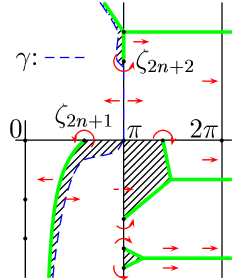
Figure 5. The continuation diagram

Let $D=\{|{\rm Im}\,\zeta|\leq Y,\,\,\,0<{\rm Re}\,\zeta<2\pi\}$ ($Y$ is as in Proposition 4.2). Consider also $D^{\prime}$, the domain obtained from $D$ by cutting it along segments of Stokes lines and along lines ${\rm Re}\,\zeta={\rm Const}$ as shown in Fig. 5. Note that, we have cut away (i.e. $D^{\prime}$ does not contain) the part of $D$ situated to right of the Stokes line “c” (see Fig. 3). The domain $D^{\prime}$ is simply connected; thus, both the branch $\kappa$ and the leading term of the standard asymptotics of $f$ can be analytically continued on $D^{\prime}$ in a unique way. Using the continuation principles, we prove

Proposition 6.1.

If $\delta$ (from Proposition 4.2) is chosen sufficiently
small, then, inside $D^{\prime}$, the solution $f$ has the standard behavior

$$\hskip-113.81102ptf\sim\exp\left(\frac{i}{\varepsilon}\int_{\pi}^{\zeta}\kappa d\zeta\right)\,\Psi_{+}.$$

The rest of this section devoted to the proof of this proposition. The proof is naturally divided into “elementary” steps. In each step, applying just one of the three continuation tools (i.e. the Rectangle Lemma, the Adjacent Canonical Domain Principle and the Stokes Lemma), we extend the continuation diagram, justifying the standard behavior of $f$ on a larger subdomain of $D^{\prime}$. Fig. 5 shows where we use each of the continuation principles. The full straight arrows indicate the use of the Rectangle Lemma, the circular arrows, the use of the Stokes Lemma, and, the dashed arrows and the hatched zones, the use of the Adjacent Canonical Domain Principle. When proving Proposition 6.1, one repeats the same arguments quite often. So, we explain in details only the first few steps of the proof to show how to use each of the continuation tools.

6.1. Behavior of $\mathbf{f}$ between the lines $\mathbf{\gamma}$ and $\mathbf{\beta}$: applying the Adjacent Canonical Domain Principle

Recall that $\gamma$ first goes downwards staying to the left of $\beta$, and, then, $\gamma$ and $\beta$ meet at a point $a$, $0<{\rm Im}\,a<{\rm Im}\,\zeta_{2n+2}$. They coincide up to a point $b$, ${\rm Im}\,b<0$. Here, by means of the Adjacent Canonical Domain Principle, we prove that $f$ has the standard behavior inside a subdomain of $D$ situated above $a$ between $\gamma$ and $\beta$. Our strategy is the following. First, we use the Trapezium Lemma, Lemma 5.4, to describe a part of a canonical domain enclosing to the upper part of $\gamma$, and, then, we use the Adjacent Canonical Domain Principle.

6.1.1. Describing $U$, $\gamma_{0}$, $\sigma_{u}$ and $\sigma_{d}$

Let us describe the domain $U$ and the curves $\gamma_{0}$, $\sigma_{d}$ and $\sigma_{u}$ needed to apply Lemma 5.4.

The domain $U$. It is the domain bounded by $\beta$, $\gamma$ and the line ${\rm Im}\,\zeta={\rm Const}$ containing the upper end of $\gamma$. Inside $U$, one has ${\rm Im}\,\kappa>0$.

The line $\sigma_{u}$. As $\sigma_{u}$, we take the line which intersects $\beta$ at $\tilde{\zeta}_{u}$, the point with the imaginary part equal to $Y$, and belongs to the family ${\rm Im}\,\int^{\zeta}\kappa d\zeta={\rm Const}$. Recall that $\gamma$ is constructed in the $\delta$-neighborhood of $\beta$ where $\delta$ can be fixed arbitrarily small. One has

Lemma 6.1.

The line $\sigma_{u}$ enters $U$ at the point $\tilde{\zeta}_{u}$ and goes upwards. If $\delta$ is sufficiently small, then, $\sigma_{u}$ intersects $\gamma$ at $\zeta_{u}$, an internal point of $\gamma$.

Proof.  Recall that $Y>{\rm Im}\,\zeta_{2n+3}$, and that, above $\zeta_{2n+3}$, $\beta$ coincides with the Stokes line “c” tangent to the vector field $\overline{\kappa(\zeta)-\pi}$. The line $\sigma_{u}$ is tangent to the vector field $\overline{\kappa(\zeta)}$. One has ${\rm Im}\,\kappa(\tilde{\zeta}_{u})>0$. Therefore, at $\tilde{\zeta}_{u}$, the tangent vector to $\beta$ (oriented upwards) is directed to the left with respect to the tangent vector to $\sigma_{u}$ (oriented upwards). So, $\sigma_{u}$ enters $U$ at $\tilde{\zeta}_{u}$ going upwards. As ${\rm Im}\,\kappa\neq 0$ in $U$, $\sigma_{u}$ stays vertical (in $U$). As $\sigma_{u}$ is independent of $\delta$, if $\delta$ is sufficiently small, $\sigma_{u}$ intersects $\gamma$. This completes the proof of Lemma 6.1.∎

The line $\sigma_{d}$. It is the line which intersects $\beta$ at $\tilde{\zeta}_{d}$, a point such that ${\rm Im}\,a<\tilde{\zeta}_{d}<{\rm Im}\,\zeta_{2n+2}$, and belongs to the family ${\rm Im}\,\int^{\zeta}(\kappa-\pi)d\zeta={\rm Const}$. One has

Lemma 6.2.

The line $\sigma_{d}$ enters $U$ at $\tilde{\zeta}_{d}$, goes downwards and then, staying in $U$, it intersects $\gamma$ at a point $\zeta_{d}$. This point can be made arbitrarily close to $a$ by choosing $\tilde{\zeta}_{d}$ sufficiently close to $a$.

Proof.  Recall that the segment $[\pi,\zeta_{2n+2}]$ of the line ${\rm Re}\,\zeta=\pi$ belongs to the pre-image (by $\mathcal{E}$) of the $(n+1)$-st spectral band of the periodic operator. So, ${\rm Im}\,\kappa=0$ and $0<{\rm Re}\,\kappa<\pi$ on $[\pi,\zeta_{2n+2}]$. Moreover, in $U$, one has ${\rm Im}\,\kappa>0$. As $\sigma_{d}$ is tangent to the vector field $\overline{\kappa}-\pi$, arguing as usual, we deduce from these properties of $\kappa$ that

1. $\sigma_{d}$ is orthogonal to $\beta$ at $\tilde{\zeta}_{d}$, enters $U$ at this point;

2. having entered $U$, it goes downwards and stays vertical while in $U$;

3. it leaves $U$ intersecting $\gamma$.

Being an integral curve of a smooth vector field, $\sigma_{d}$ intersects $\gamma$ as close to $a$ as desired provided that $\tilde{\zeta}_{d}$ is sufficiently close to $a$. This completes the proof of Lemma 6.2.∎

The line $\gamma_{0}$. We choose $\delta$ so that $\sigma_{u}$ intersect $\gamma$. Then, $\gamma_{0}$ is the segment of $\gamma$ between its intersections with $\sigma_{d}$ and $\sigma_{u}$.

6.1.2. Describing the curve $\tilde{\gamma}$

We shall use the first variant of the Trapezium Lemma (i.e. the first point of Lemma 5.4). Let us describe the canonical line $\tilde{\gamma}$ needed to apply it. In Proposition 4.3, we have constructed $\gamma$ by means of Proposition 4.2. In the same way, we can construct another canonical line situated arbitrarily close to $\beta$. So, we can assume that it is strictly between $\gamma_{0}$ and $\beta$. This canonical line is the one we use as $\tilde{\gamma}$.
As $\sigma_{u}$ and $\sigma_{d}$ intersect $\gamma$ and $\beta$, they also intersect $\tilde{\gamma}$.

6.1.3. Completing the analysis

By the Trapezium Lemma, the domain bounded by $\gamma_{0}$, $\sigma_{u}$, $\sigma_{d}$ and $\tilde{\gamma}$ is a part of a canonical domain enclosing $\gamma_{0}$. So, by the Adjacent Domain Canonical Principle, $f$ has the standard behavior here.
As $\zeta_{d}$ can be chosen arbitrarily close to $a$ and $\tilde{\gamma}$ can be constructed arbitrarily close to $\beta$, we conclude that $f$ has the standard behavior in the domain bounded by $\beta$, $\gamma$ and the line ${\rm Im}\,\zeta=Y$.

6.2. “Crossing” the segment $\mathbf{[0,\zeta_{2n+2}]\subset\beta}$: another example of how to use the Adjacent Canonical Domain Principle

Pick $c$ so that $0\leq c<{\rm Im}\,\zeta_{2n+2}$. Let $s_{c}$ be the segment $[0,\zeta_{2n+2}-c]$ of the line $\beta$ (i.e of the line ${\rm Re}\,\zeta=\pi$). We shall check

Lemma 6.3.

For $c>0$,  $s_{c}$ is a canonical line.

This and the Adjacent Canonical Domain Principle will imply

Lemma 6.4.

The solution $f$ has standard behavior in a neighborhood of any internal point of $s_{0}$ (i.e. $s_{c}$ with $c=0$).

Proof.  Indeed, let $c>0$. As, $I_{c}$ is canonical, by Lemma 4.1, there is $K_{c}$, a canonical domain enclosing $s_{c}$. Moreover, by the previous step, see section 6.1.3, $f$ has the standard behavior to the left of $s_{c}$. Applying the Adjacent Canonical Domain Principle, we prove that $f$ has standard behavior in $K_{c}$. As $c$ can be taken arbitrarily small, we obtain Lemma 6.4. ∎

Before proving Lemma 6.3, note that $s_{0}$ contains the branch point $\zeta_{2n+2}$. So, $s_{0}$ itself cannot be a canonical line.

Proof of Lemma 6.3. Note that $s_{c}\subset z_{n+1}$, i.e. $s_{c}$ is a part of a connected component of the pre-image of the $(n+1)$-st spectral band of the periodic operator (0.3) with respect to the mapping $\mathcal{E}:\,\zeta\to E-W(\zeta)$. For $c>0$, $\mathcal{E}$ maps $s_{c}$ strictly into the $(n+1)$-st spectral band. This implies that, along $s_{c}$, one has $0<k(\zeta)<\pi$. Now, Lemma 6.3 follows from the definition of canonical lines. ∎

6.3. Behavior of $\mathbf{f}$ to the right of $\mathbf{s_{0}}$: using the Rectangle Lemma

Let $R_{0}$ be the rectangle bounded by the real line, the segment $s_{0}$, the line ${\rm Im}\,\zeta={\rm Im}\,\zeta_{2n+2}$ and the line ${\rm Re}\,\zeta=2\pi$. By means of the Rectangle Lemma, we prove

Lemma 6.5.

Inside $R_{0}$, the solution $f$ has the standard behavior.

Proof.  First, we note that, in the interior of $R_{0}$, one has ${\rm Im}\,\kappa<0$. Indeed, ${\rm Im}\,\kappa$ vanishes only at points of the pre-image of the set of spectral bands of the periodic operator with respect to $\mathcal{E}$. Therefore, in the interior of $R_{0}$, one has ${\rm Im}\,\kappa\neq 0$. Furthermore, in $\Pi$, the imaginary part of $\kappa$ is positive, and to go from $\Pi$ to $R_{0}$ (while staying inside $D^{\prime}$), one has to intersect $s_{0}$, i.e. a connected component of the pre-image of the $(n+1)$-st spectral band. So, in the interior of $R_{0}$, the imaginary part of $\kappa$ is negative.
Now, fix $c$, a sufficiently small positive constant. Consider the closed “rectangle” $R_{c}\subset R_{0}$ delimited by the lines ${\rm Re}\,\zeta=\pi$, ${\rm Im}\,\zeta=c$, the line ${\rm Re}\,\zeta=2\pi-c$ and the line ${\rm Im}\,\zeta={\rm Im}\,\zeta_{2n+2}-c$. As $R_{c}\subset R_{0}$, the imaginary part of $\kappa$ is negative in $R_{c}$. Moreover, by Lemma 6.4, the solution $f$ has the standard behavior $f\sim e^{\frac{i}{\varepsilon}\int_{\pi}^{\zeta}\kappa d\zeta}\Psi_{+}$ in a neighborhood of the left boundary of $R_{c}$. So, the rectangle $R_{c}$ satisfies the assumptions of the Rectangle Lemma, and, therefore, $f$ has the standard behavior inside $R_{c}$. As $c$ can be taken arbitrarily small, this implies that $f$ has standard asymptotics inside the whole rectangle $R_{0}$. ∎

6.4. Applying the Stokes Lemma

Recall that the segment $\sigma=[\zeta_{2n+2},\zeta_{2n+3}]$ of the line ${\rm Re}\,\zeta=\pi$ is a Stokes line. By the previous steps, we know that, at least near $\sigma$, the solution $f$ has the standard behavior to the left of and below $\sigma$. To justify the standard behavior of $f$ to the right of $\sigma$, one uses the Stokes Lemma.
Let $V$ be a neighborhood of $\sigma$. Pick $c$ so that $0<c<{\rm Im}\,(\zeta_{2n+3}-\zeta_{2n+2})$. Let $V_{c}=\{\zeta\in V,\,\,{\rm Im}\,\zeta<{\rm Im}\,\zeta_{2n+3}-c\}$. We prove

Lemma 6.6.

If $V$ is sufficiently small, $f$ has the standard behavior in $V_{c}\setminus\sigma$.

Proof.  There are three Stokes lines beginning at $\zeta_{2n+2}$. These are the lines $\sigma$, “b” and the line “$\tilde{\rm b}$” symmetric to “b” with respect to the line ${\rm Re}\,\zeta=\pi$. Suppose that $V$ is chosen sufficiently small. Then,

1. the three Stokes lines divide $V_{c}$ into three sectors;

2. by the first three steps of the continuation process, we know that $f$ has the standard behavior outside the sector bounded by $\sigma$ and “$\tilde{\rm b}$”;

3. in $V_{c}$, to the left of $\sigma$,  ${\rm Im}\,\kappa>0$.

So, the conditions of the Stokes Lemma are satisfied, and, therefore, $f$ has the standard behavior in $V_{c}\setminus\sigma$. This completes the proof of Lemma 6.6.∎

6.5. Completing the analysis of $\mathbf{f}$ in $\mathbf{D^{\prime}}$

One completes the analysis of $f$ using our continuation tools as indicated in Fig. 5. Applying each of the continuation principles, one argues essentially as in the previous steps. Let us outline the analysis concentrating only on the new elements.

6.5.1. The solution $f$ in $D^{\prime}\cap{\mathbb{C}}_{+}$

By means of the Rectangle Lemma, one justifies the standard behavior of $f$ first to the left of $\gamma$ and, second, to the right of the line ${\rm Re}\,\zeta=\pi$.

6.5.2. Beginning the analysis of $f$ in $D^{\prime}\cap{\mathbb{C}}_{-}$: standard steps

1.  One begins with justifying the standard behavior between the lines $\beta$ and $\gamma$ below the real line. Therefore, one uses the Adjacent Canonical Domain Principle.
2.  Then, one “continues the asymptotics” of $f$ to the right of $\gamma$. First, one tries to use the Rectangle Lemma. However, on the line ${\rm Re}\,\zeta=\pi$, one meets a problem: ${\rm Im}\,\kappa=0$ on the segments $s_{n+1}=[\pi,\bar{\zeta}_{2(n+1)}]$ and $s_{j}=[\bar{\zeta}_{2j-1},\bar{\zeta}_{2j}]$ for $j=n+2,\,n+3\dots$. Indeed, $s_{j}$ is a connected component of the pre-image of the $j$-th spectral band of the periodic operator.
In result, one obtains standard behavior by means of the Rectangle Lemma only outside the domains

$$d_{j}=\{\zeta=s+t,\,s\in s_{j},\,\,\pi\leq t<2\pi\},\quad j=n+1,n+2\dots.$$

3.  Consider the hatched domains in Fig. 5. Each of them is adjacent to one of the segments $s_{j}$ and bounded by Stokes lines. Denote by $T_{j}$ the hatched domain adjacent to $s_{j}$. One justifies the standard behavior in $T_{j}$ by means of the Adjacent Domain Principle and the second variant of the Trapezium Lemma (second point of Lemma 5.4). Let us describe the domain $U$ and the lines $\gamma_{0}$, $\sigma_{u}$ and $\sigma_{d}$ needed to apply the Trapezium Lemma to study $f$ in $T_{j}$.
The line $\gamma_{0}$.  Let $\zeta_{u}$ and $\zeta_{d}$ be two internal points of $s_{j}$ such that ${\rm Im}\,\zeta_{d}<{\rm Im}\,\zeta_{u}$. The line $\gamma_{0}$ is the segment $[\zeta_{d},\zeta_{u}]$ of $s_{j}$. We define the branch of the complex momentum with respect to which $\gamma_{0}$ is a canonical line. Therefore, we note that $\pi(j-1)<\kappa+\pi n<\pi j$ as $\zeta$ is inside $s_{j}$ and set

(6.1) $$\kappa_{j}=\left\{\begin{array}[]{c}\kappa+\pi n-\pi(j-1),\quad\text{if \ }j\text{\ is \ odd},\\ \pi j-\pi n-\kappa,\quad\text{otherwise}.\end{array}\right.$$

As seen from the section 2.1.2, the function $\kappa_{j}$ is a branch of the complex momentum. Along $s_{j}$, one has $0<\kappa_{j}<\pi$. This implies that $\gamma_{0}$ is a canonical line with respect to $\kappa_{j}$.
For sake of definiteness, below, we assume that $j$ is odd. The case $j$ even is treated similarly.
The domain $U$. It is a subdomain of $T_{j}$. In $T_{j}$, one has ${\rm Im}\,\kappa_{j}>0$. Indeed, to go from $\Pi$ to $T_{j}$, one has to twice intersect connected components of the pre-image (with respect to $\mathcal{E}$) of the set of the spectral bands. So, in $T_{j}$, one has ${\rm Im}\,\kappa>0$. As $j$ is odd, (6.1) implies that ${\rm Im}\,\kappa_{j}>0$ in $T_{j}$.
The lines $\sigma_{u}$ and $\sigma_{d}$. They are respectively defined by the relations ${\rm Im}\,\int_{\zeta_{u}}^{\zeta}\kappa_{j}d\zeta=0$ and ${\rm Im}\,\int_{\zeta_{d}}^{\zeta}(\kappa_{j}-\pi)d\zeta=0$. Note that, $\sigma_{d}$ contains $\zeta_{d}$, and $\sigma_{u}$ contains $\zeta_{u}$. So, if $\zeta_{d}$ and $\zeta_{u}$ would be respectively the lower and the upper end of $s_{j}$, then, the lines $\sigma_{u}$ and $\sigma_{d}$ are the lines of Stokes type bounding $T_{j}$.
By means of Lemma 2.1, one proves that, in $T_{j}$, the lines $\sigma_{u}$ and $\sigma_{d}$ are vertical, $\sigma_{u}$ is going downward from $\zeta_{u}$, and $\sigma_{d}$ is going upward from $\zeta_{d}$.
Finally, one checks that, having entered in $T_{j}$, the lines $\sigma_{u}$ and $\sigma_{d}$ intersect one another before leaving $T_{j}$. Indeed, Lemma 5.5 implies that the line $\sigma_{d}$ (resp. $\sigma_{u}$) can leave $T_{j}$ only intersecting its upper (resp. lower) boundary.
Completing the analysis. The Trapezium Lemma implies that the domain bounded by $\gamma_{0}$, $\sigma_{d}$ and $\sigma_{u}$ is a part of a canonical domain enclosing $\gamma_{0}$. Therefore, by Adjacent Canonical Domain Principle, $f$ has the standard behavior in this domain. Note that, as $\zeta_{u}$ and $\zeta_{d}$ approach the upper and lower ends of $s_{j}$, the curves $\sigma_{u}$ and $\sigma_{d}$ approach the upper and lower boundary of $T_{j}$. This implies that, in fact, $f$ has the standard behavior inside the whole domain $T_{j}$.
4.  One justifies the standard behavior of $f$ to the left of the hatched domains using the Stokes Lemma and the Rectangle Lemma (see Fig. 5). We omit the details and note only that, to do this to the right of $T_{n+1}$, one first has to check that $f$ has the standard behavior along the interval $(\zeta_{2n+1},2\pi-\zeta_{2n+1})$ of the real line (this was not done before!). We do this in the next subsection.

6.5.3. The analysis of $f$ in $D^{\prime}$ and along the interval $(\zeta_{2n+1},2\pi-\zeta_{2n+1})$ of the real line

First, as $f$ has the standard behavior in a neighborhood of $\gamma$, it has the standard behavior in a neighborhood of $\zeta=\pi$, the point of intersection of $\gamma$ and the real line. Hence, there exists a point $a$ such that $\zeta_{2n+1}\leq a<\pi$ such that $f$ has the standard behavior in a neighborhood of any point situated between $\pi$ and $a$, but not at $a$. Assume that $a>\zeta_{2n+1}$. Let $\alpha$ be the segment of the line ${\rm Re}\,\zeta=a$ connecting a point $a_{1}\in{\mathbb{C}}_{-}$ to a point $a_{2}\in{\mathbb{C}}_{+}$. One has $0<\kappa(a)<\pi$. So, if $\alpha$ is sufficiently small, it is canonical. The solution $f$ has the standard behavior to the right of $\alpha$ (this follows from the definition of $a$ and the previous analysis). So, we are in the case of the Adjacent Canonical Domain Principle; it implies that $f$ has the standard behavior in a local canonical domain enclosing $\alpha$. Therefore, $f$ has the standard behavior in a constant neighborhood of $a$. So, we obtain a contradiction, and, thus $a=\zeta_{2n+1}$. This completes the analysis of $f$ along the interval $(\zeta_{2n+1},\pi)$. Similarly one studies $f$ along $(\pi,2\pi-\zeta_{2n+1})$.

6.5.4. Completing the proof

We still have to check that $f$ has the standard behavior to the left of the Stokes line $\overline{\text{``a''}}$ symmetric to “a” with respect to the real line. Therefore, one first uses the Stokes Lemma to justify the standard behavior in the left hand side of a small neighborhood of $\overline{\text{``a''}}$, and, then, one uses The Rectangle Lemma to justify the standard behavior in the rest of the part of $D^{\prime}$ situated to the left of $\overline{\text{``a''}}$.
This completes the analysis of the behavior of $f$ in the domain $D^{\prime}$.∎

7. Behavior of solutions outside the continuation diagrams

In this section, we formulate and prove the Two-Waves Principle.

7.1. Formulation of the problem

7.1.1. Geometry of the problem

Assume that for $E=E_{0}$, one has the geometrical situation shown in part a) of Fig. 6. There, $\zeta_{1}$ and $\zeta_{2}$ are two branch points of the complex momentum such that $W^{\prime}(\zeta_{1})$ and $W^{\prime}(\zeta_{2})$ are non zero. The line $\sigma_{1}$ is simultaneously a Stokes line beginning at $\zeta_{1}$ and at $\zeta_{2}$. The line $\sigma_{2}$ is a segment of a Stokes line beginning at $\zeta_{2}$. We assume that both $\sigma_{1}$ and $\sigma_{2}$ are vertical.

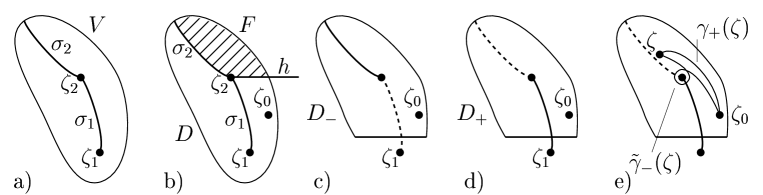
Figure 6. The Two-Waves Principle

Let $V$ be a neighborhood of $\sigma_{1}\cup\sigma_{2}$ containing only two branch points, precisely $\zeta_{1}$ and $\zeta_{2}$. Let $h=\{\zeta:\,\,{\rm Im}\,\zeta=\zeta_{2},\,\,{\rm Re}\,\zeta>{\rm Re}\,\zeta_{2}\}$. Also, denote by $F$ the part of $V$ situated above $h$ and to the right of $\sigma_{2}$ , see Fig. 6, b).

7.1.2. Formulation of the problem

Pick $\zeta_{0}\in V$ so that $\mathcal{E}(\zeta_{0})\not\in P\cup Q$. Assume that a solution $f$ has the standard behavior $f\sim\exp\left(\frac{i}{\varepsilon}\int_{\zeta_{0}}^{\zeta}\kappa\,d\zeta\right)\cdot\Psi_{+}$ in the domain $D=V\setminus(F\cup\sigma_{1})$. Assume, moreover, that the imaginary part of $\kappa$ is positive in $D$ to the left of $\sigma_{1}\cup\sigma_{2}$. Our aim is then to describe $f$ in the domain $F$.

The problem described above comes about in the case studied in section 6. The lines $\sigma_{1}$ and $\sigma_{2}$ are respectively the Stokes lines $[\zeta_{2n+2},\zeta_{2n+3}]$ and “c”, and the domain $F$ is situated to the right of “c” above the line ${\rm Im}\,\zeta={\rm Im}\,\zeta_{2n+3}$, see Fig. 5.

7.2. Two-Waves Principle

The natural idea is to try to represent $f$ as a linear combination of solutions having standard behavior in $F$. This leads to the following construction.

Consider $D_{\pm}$, the subdomains of $V$ shown in Fig. 6, parts c) and d). On each of them, fix the branch of the complex momentum so that, in some neighborhood of $\zeta_{0}$, it coincide with the branch from the asymptotics of $f$. It will be convenient to assume that $\zeta_{0}$ is to the right of $\sigma_{1}\cup\sigma_{2}$. One has

Lemma 7.1 (Two-Waves Principle).

Assume that there are two solutions $h_{\pm}$ having the standard behavior $h_{\pm}\sim\exp(\pm\frac{i}{\varepsilon}\int_{\zeta_{0}}^{\zeta}\kappa\,d\zeta)\cdot\Psi_{\pm}$ in $D_{\pm}$. Then,

(7.1) $$f(\zeta)=g(\zeta)\,h_{+}(\zeta)+G(\zeta)\,h_{-}(\zeta),\quad\zeta\in F,$$

where $\zeta\mapsto G(\zeta)$ and $\zeta\mapsto g(\zeta)$ are two $\varepsilon$-periodic functions. In $F$, these functions admit the asymptotic representations

Figure 7. The curves $\gamma^{0}$ and $\gamma_{-}^{0}$

(7.2) $$\begin{split}\hskip-142.26378ptG&=e^{\textstyle\frac{2i\kappa(\zeta_{2})}{\varepsilon}\,(\zeta-\zeta_{2})}\,\,\frac{(A-1+o(1))}{B}\,\,(1+o(1)),\\ \hskip-142.26378ptg&=1+o(1),\end{split}$$

where $A$ and $B$ are constants given by the formulae

(7.3) $$\begin{split}\hskip-142.26378ptA&=\exp\left(\frac{i}{\varepsilon}\,\oint_{\gamma_{0}}\kappa d\zeta+\oint_{\gamma_{0}}\Omega_{+}+\text{ind}\,(\gamma_{0})\right),\\ \hskip-142.26378ptB&=\exp\left(-\frac{i}{\varepsilon}\oint_{\gamma_{-}^{0}}\kappa d\zeta+\oint_{\gamma_{-}^{0}}\Omega_{-}+\text{ind}\,(\gamma_{-}^{0})\right).\end{split}$$

Here, $\gamma_{0}$ and $\gamma_{-}^{0}$ are loops going around the branch point as shown in Fig. 7 and do not containing any points of ${\mathcal{E}}(P\cup Q)$;  $\text{ind}\,(\alpha)$ denotes the increment of $\arg\left(\sqrt{k^{\prime}({\mathcal{E}}(\zeta))}\right)$ along a closed curve $\alpha$. The representations (7.2) are uniform in $\zeta$ and $E$ provided that $\zeta$ is in a compact subset of $F$ and $E$ is in a sufficiently small neighborhood of $E_{0}$.

7.3. Comments and remarks

Let us comment on the Two-Waves Principle.

7.3.1. Solutions $h_{\pm}$

Recall that $V$ is a neighborhood of $\sigma_{1}\cup\sigma_{2}$. If $V$ is sufficiently small (and, thus, “thin” and “stretched” along $\sigma_{1}$ and $\sigma_{2}$), the solutions $h_{\pm}$ can be easily constructed using our standard techniques. However, in practice, one does not use these local constructions. Instead, one tries to construct $h_{\pm}$ so that they have the standard behavior on domains as large as possible. Thus, their construction is determined by the concrete geometry of the problem. Detailed examples can be found in section 7.4.

7.3.2. A convenient representation for $f$

We have formulated the Two-Waves Principle in terms of the solutions $h_{\pm}$ to simplify the exposition. However, to makes the results more transparent, let us change the normalization of $h_{-}$. Let

$$h_{-}^{o}=e^{\frac{2i\kappa(\zeta_{2})}{\varepsilon}\,(\zeta-\zeta_{2})}\,B^{-1}\,h_{-}.$$

It will follow from the proof of Lemma 7.1 that the solution $h_{-}^{o}$ has the standard behavior

(7.4) $$h_{-}^{o}\sim e^{\frac{i}{\varepsilon}\int_{\tilde{\gamma}_{-}(\zeta)}\kappa\,d\zeta}\Psi_{+},\quad\quad\zeta\in F,$$

where the curve $\tilde{\gamma}_{-}$ is shown in Fig. 6, part e), and $\kappa$ and $\Psi_{+}$ are obtained by the analytic continuation from $\zeta_{0}$ along $\tilde{\gamma}_{-}$. In terms of the solutions $h_{+}$ and $h_{-}^{o}$, formula (7.1) takes the simplest form

(7.5) $$f=h_{+}(1+o(1))+[A-1+o(1)]\,h_{-}^{o}\,(1+o(1)).$$

Note that, for small $\varepsilon$, the absolute values of $h_{+}$ and $h_{-}^{o}$ are essentially determined by the factors

(7.6) $$\exp\left(\frac{i}{\varepsilon}\int_{\gamma_{+}(\zeta)}\kappa\,d\zeta\right)\quad\text{and}\quad\exp\left(\frac{i}{\varepsilon}\int_{\tilde{\gamma}_{-}(\zeta)}\kappa\,d\zeta\right),$$

where $\gamma_{+}(\zeta)$ is shown in Fig. 6, part e). The definition of Stokes lines implies that, along the Stokes lines beginning at $\zeta_{2}$, the moduli of these factors are equal.

7.3.3. The coefficient $A$

The coefficient $A$ is defined in $U$, a sufficiently small constant neighborhood of $E_{0}$. Formula (7.5) shows that it is important to compare the modulus of $A$ with $1$. For $\varepsilon$ small, the modulus of $A$ is essentially determined by the factor $\exp\left(-\frac{1}{\varepsilon}\,{\rm Im}\,\,\oint_{\gamma_{0}}\kappa d\zeta\right)$. So, when $\varepsilon\to 0$, depending of $E\in U$, the coefficient $A$ may become exponentially small or exponentially large. However, for some $E\in U$, it always is of order $O(1)$. Indeed, one proves

Lemma 7.2.

Fix $E\in U$. Assume that the configuration of the Stokes lines corresponds Fig. 6, part a). Then, one has ${\rm Im}\,\,\oint_{\gamma_{0}}\kappa d\zeta=0$.

Proof.  Fix $E$ as in Lemma 7.2 and consider $\kappa$ as a function of $\zeta\in V$ ($V$ is the neighborhood of $\sigma_{1}\cup\sigma_{2}$ defined in section 7.1.2). Cut $V$ along $\sigma_{1}$. First, we check that the branch of $\kappa$ (defined in a neighborhood of $\zeta_{0}$) is analytic $V\setminus\sigma_{1}$. Consider the curve $\gamma$ beginning at $\zeta_{0}$ and going to $\sigma_{1}$ along a straight line, then, going around $\sigma_{1}$ just along it (infinitesimally close to it) and, finally, coming back to $\zeta_{0}$ along the same straight line. Continue $\kappa$ analytically along $\gamma$. Relation (2.5) implies that, near $\zeta_{0}$, the values of $\kappa$ and of its analytic continuation differ by the additive constant $2(\kappa(\zeta_{1})-\kappa(\zeta_{2}))$. But, as $\sigma_{1}$ is a Stokes line for both $\zeta_{1}$ and $\zeta_{2}$, one has $\kappa(\zeta_{1})=\kappa(\zeta_{2})$. This implies the analyticity of $\kappa$.

As $\kappa$ is single valued in $V\setminus\sigma_{1}$, we can deform the integration contour $\gamma_{0}$ from the definition of $A$ so that it go around $\sigma_{1}$ just along it. Now, it follows from the definition of the Stokes lines that ${\rm Im}\,\oint_{\gamma_{0}}\kappa d\zeta={\rm Im}\,\oint_{\gamma_{0}}(\kappa(\zeta)-\kappa(\zeta_{1}))d\zeta=0$. ∎

7.3.4. Generalizations of the Two-Waves Principle

In the same way as we prove Lemma 7.1, one obtains analogous statements for the “symmetric” geometries shown in Fig. 8.

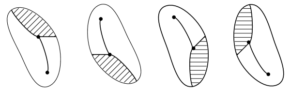
Figure 8. All the possible geometric situations

7.4. How to use the Two-Waves Principle: an example

Consider the solution $f$ studied in section 6. We now apply the Two-Waves Principle to obtain the asymptotics of $f$ to the right of the Stokes line “c”.

7.4.1. Comparing the notations

The points $\zeta_{1}$ and $\zeta_{2}$ are the branch points $\zeta_{2n+2}$ and $\zeta_{2n+3}$; the Stokes lines $\sigma_{1}$ and $\sigma_{2}$ are the Stokes lines $[\zeta_{2n+2},\zeta_{2n+3}]$ and “c” (more precisely, its segment below the line ${\rm Im}\,\zeta=Y$, $Y>{\rm Im}\,\zeta_{2n+3}$). The domain $F$ situated above the line ${\rm Im}\,\zeta={\rm Im}\,\zeta_{2n+3}$ and to the right of “c”.

7.4.2. Checking the assumptions of the Two-Waves Principle

The assumptions of Lemma 7.1 are satisfied: $\sigma_{1}$ is a Stokes line both for $\zeta_{2n+2}$ and $\zeta_{2n+3}$; both $\sigma_{1}$ and $\sigma_{2}$ are vertical; $f$ has the standard behavior in $V\setminus(F\cup[\zeta_{2n+2},\zeta_{2n+3}])$; and, to the left of the Stokes lines “c” and $[\zeta_{2n+2},\zeta_{2n+3}]$, near them, one has ${\rm Im}\,\kappa>0$.

7.4.3. The solution $h_{+}$

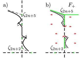
(a) The construction of $h_{+}$

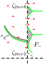
(b) and of $h_{-}$

Figure 9. Constructions of $h_{\pm}$

To construct the solution $h_{+}$, we first build $\pi_{+}$, a pre-canonical line, as shown in Fig. 9(a), part a). When speaking about $\kappa$ on $\pi_{+}$, we mean the branch of the complex momentum obtained by analytic continuation of the branch $\kappa$ from the asymptotics of $f$ along $\pi_{+}$ from $D^{\prime}$. Actually, $\pi_{+}$ is pre-canonical with respect to $\kappa_{1}$, the branch of the complex momentum equal to $2\pi-\kappa$. The construction of $\pi_{+}$ being standard, we omit details and note only that $\pi_{+}$ consists of five “elementary” segments. The first (the lower) “elementary” segment and the fourth one are segments of lines of Stokes type ${\rm Im}\,\int^{\zeta}(\kappa_{1}-\pi)d\zeta={\rm Const}$. The second and the fifth ones are segments of lines of Stokes type ${\rm Im}\,\int^{\zeta}\kappa_{1}d\zeta={\rm Const}$. The third elementary segment is a canonical line.
Having constructed $\pi_{+}$, we pick $\gamma_{+}$, a canonical line close to $\pi_{+}$, and, by Theorem 3.1, construct the solution $g\sim e^{-\frac{i}{\varepsilon}\int_{\pi}^{\zeta}\kappa_{1}d\zeta}$ on $K_{+}$, a canonical domain enclosing this canonical line.
We let $h_{+}=\exp\left(\frac{2\pi i(\zeta-\pi)}{\varepsilon}\right)g$. On $K_{+}$, the function $h_{+}$ has the standard behavior $h_{+}\sim e^{\frac{i}{\varepsilon}\int_{\pi}^{\zeta}\kappa d\zeta}\Psi_{+}$.
The computation of the continuation diagram of $h_{+}$ is explained in Fig. 9(a), part b), where we show only what happens in the domain $0<{\rm Re}\,\zeta<2\pi$.
Note that we do not control the behavior of $h_{+}$ in the domain denoted by $F_{+}$ in Fig. 9(a), part b).

7.4.4. The solution $h_{-}$

To construct $h_{-}$, we build $\pi_{-}$, a pre-canonical line similarly to $\pi_{+}$. The only difference is that, above the point $\zeta_{2n+3}$, instead of going along the line ${\rm Re}\,\zeta=\pi$ to a neighborhood of $\zeta_{2n+4}$ , the pre-canonical line $\pi_{-}$ goes along a line of Stokes type ${\rm Im}\,\int^{\zeta}(\kappa_{1}-\pi)d\zeta={\rm Const}$ which belongs to the same family as “c”, is situated to the right of “c” and is chosen sufficiently close to “c”.
On $K_{-}$, a canonical domain enclosing $\gamma_{-}$, a canonical line “approximating” $\pi_{-}$, the solution $h_{-}$ has the standard behavior $h_{-}\sim e^{-\frac{i}{\varepsilon}\int_{\pi}^{\zeta}\kappa d\zeta}\Psi_{-}$.
The analysis of the continuation diagram of $h_{-}$ is explained in Fig. 9(b), where we show only what happens in the domain $0<{\rm Re}\,\zeta<2\pi$.
Note that we do not control the behavior of $h_{-}$ in the domain denoted by $F_{-}$ in Fig. 9(b).

7.4.5. Asymptotics of $f$

As in section 7.3.2, in terms of $h_{-}$, we define the solution $h_{-}^{o}$. By the Two-Wave Principle, $f$ admits the representation (7.5). This yields the asymptotics of $f$ in $F$.
This leaves us with the following two questions:

• what is the asymptotics of $f$ in the domain $F\cap F_{+}$ (where the asymptotics $h_{+}$ is unknown)?

• how to get the asymptotics of $f$ in the domain $F\cap F_{-}$ (where the asymptotics $h_{-}$ is unknown)?

Denote by $\alpha$ the Stokes line beginning at $\zeta_{2n+5}$ and going from it upwards to the left. To answer the first question, one has to find the asymptotics of $h_{+}$ in the domain $F_{+}$ situated to the right of $\alpha$ and above the line ${\rm Im}\,\zeta={\rm Im}\,\zeta_{2n+5}$. Therefore, one has just to apply the Two-Waves Principle once more (now, to study $h_{+}$).

Denote by $\beta$ the Stokes line beginning at $\zeta_{2n+3}$ going upwards to the right. Denote by $p$ the point where it intersects the Stokes line beginning at $\zeta_{2n+4}$ going downwards to the right. The answer to the second question is given by

Lemma 7.3.

Let $D_{1}=\{\pi<{\rm Re}\,\zeta<2\pi,\,\,\zeta_{2n+2}<{\rm Im}\,\zeta<{\rm Im}\,p\}$. Let $D_{2}$ be the part of $D_{1}$ situated to the right of $\beta$. Then, $D_{2}$ is in the continuation diagram of $f$ i.e. in $D_{2}$, $f$ has standard asymptotics.

We only explain the idea guiding the proof of this lemma and omit the technical details. The idea is the following. Both the solutions $h_{+}$ and $h_{-}^{o}$ have the standard behavior inside $D_{2}$ near $l$, the left part of the boundary of $D_{2}$. As $l$ consists of segments of Stokes lines, along $l$, the absolute values of the exponentials (7.6) determining the order of these solutions coincide. To the right of $l$, the exponential term in the asymptotics of $h_{+}$ becomes (exponentially) larger than the one in the asymptotics of $h_{-}^{o}$. This and Lemma 7.2 imply that, in $D_{2}$, near $l$ (where both $h_{+}$ and $h_{-}^{o}$ have the standard behavior), the second term in (7.5) is negligible with respect to the first one so that, there, $f$ has the standard behavior $f\sim\exp(\frac{i}{\varepsilon}\int_{\gamma_{+}(\zeta)}\kappa\,d\zeta)\cdot\Psi_{+}$. This and the Rectangle Lemma, then, imply the statement of Lemma 7.3.

8. The proof of the Trapezium Lemma

In this section we prove the Trapezium Lemma, Lemma 5.4. We check only the first point. The second one is proved similarly. We begin with studying the lines of Stokes type inside $T$.

Pick $\zeta_{0}\in T$. By Corollary 2.1, $\zeta_{0}$ belongs to exactly one line of Stokes type from the same family as $\sigma_{d}$ and to exactly one line of Stokes type from the same family as $\sigma_{u}$. We denote these lines by $\sigma_{d}(\zeta_{0})$ and $\sigma_{u}(\zeta_{0})$ respectively. One has

Lemma 8.1.

One has

• The lines $\sigma_{d}(\zeta_{0})$ and $\sigma_{u}(\zeta_{0})$ stay vertical before leaving $U$.

• Above $\zeta_{0}$, the line $\sigma_{u}(\zeta_{0})$ leaves $T$ intersecting $\gamma_{0}$ at $\zeta_{u}$, an internal point of $\gamma_{0}$.

• Below $\zeta_{0}$, the line $\sigma_{d}(\zeta_{0})$ leaves $T$ intersecting $\gamma_{0}$ at $\zeta_{d}$, an internal point of $\gamma_{0}$.

Proof.  As ${\rm Im}\,\kappa\neq 0$ in $U$, the first point of Lemma 8.1 follows from Lemma 2.1.
Let us check the second one. First, we note that $\sigma_{u}(\zeta_{0})$ cannot leave $T$ by intersecting $\sigma_{u}$, its “upper boundary”, as both lines belong to one and the same family of line of Stokes type. Second, show that it can not leave $T$ intersecting $\tilde{\gamma}$ above $\zeta_{0}$. Consider the family $\{\sigma_{u}(t)\}|_{t\in\tilde{\gamma}}$. It contains $\sigma_{u}$, the “upper boundary” of $T_{j}$, and, by assumption, $\sigma_{u}(\zeta_{0})$. By the second point of Lemma 5.3, each line from this family intersects $\tilde{\gamma}$ transversally. So, we can orient the tangent vectors at the intersection points to the right. As, in $U$, one has ${\rm Im}\,\kappa\neq 0$, either all of these vectors are oriented upwards or all of them are oriented downwards. Therefore, all the tangent vectors are directed to the right and downwards as does the tangent vector to $\sigma_{u}$ (the “upper boundary”). But, $\sigma_{u}(\zeta_{0})$ cannot go upward from $\zeta_{0}$, stay vertical and leave $T$ intersecting $\tilde{\gamma}$ in this way.
Finally, show that $\sigma_{u}(\zeta_{0})$ can not leave $T$ by intersecting $\sigma_{d}$, the “lower boundary” of $T$. Therefore, compare $t_{d}(\zeta_{0})$ and $t_{u}(\zeta_{0})$, the tangent vectors to $\sigma_{d}(\zeta_{0})$ and $\sigma_{u}(\zeta_{0})$ at $\zeta_{0}$. As in $U$, one has ${\rm Im}\,\kappa\neq 0$, we orient both the vectors upwards. As $\sigma_{u}(\zeta_{0})$ and $\sigma_{d}(\zeta_{u})$ belong to different families of Stokes lines, either, for all $\zeta_{0}\in U$, the vector $t_{d}(\zeta_{0})$ is directed to the left with respect to $t_{u}(\zeta_{0})$ or, for all $\zeta_{0}\in U$, it is directed to the right. Comparing the tangent vectors at the point of intersection of $\sigma_{d}$ and $\tilde{\gamma}$ (the lower and the right boundaries of $T$), we see that we are in the second case i.e. for all $\zeta_{0}\in U$, $t_{d}(\zeta_{0})$ is directed to the right.
Assume that $\sigma_{u}(\zeta_{0})$ leaves $T$ by intersecting $\sigma_{d}$, the “lower boundary” of $T$. As $t_{u}$ is oriented to the left of $t_{d}$, we conclude that either $\sigma_{u}(\zeta_{0})$ intersects $\sigma_{d}(\zeta_{0})$ twice, or $\sigma_{d}(\zeta_{0})$ intersects $\sigma_{d}$. By Lemma 5.5, both these events are impossible.
So, we see that, above $\zeta_{0}$, $\sigma_{u}(\zeta_{0})$ leaves $T$ intersecting $\gamma_{0}$. This is the second point of Lemma 8.1.
The third point is proved similarly.∎

To complete the proof of Lemma 5.4, we use Proposition 5.2. First, assume that ${\rm Im}\,\kappa\neq 0$ along $\gamma_{0}$. For $\zeta_{0}\in T$, consider the line $\alpha$ which consists of the segment of $\sigma_{u}(\zeta_{0})$ above $\zeta_{0}$ between $\gamma_{0}$ and $\zeta_{0}$ and of the segment of $\sigma_{d}(\zeta_{0})$ below $\zeta_{0}$ between $\zeta_{0}$ and $\gamma_{0}$. This line is a pre-canonical line containing $\zeta_{0}$ and connecting two internal point of the canonical line $\gamma_{0}$. As this line exists for any $\zeta_{0}\in T$, Proposition 5.2 implies that $T$ is part of a canonical domain enclosing $\gamma_{0}$. This completes the proof in the case under consideration. In general case, the line $\alpha$ may become horizontal (i.e. not vertical) at its end points (recall that pre-canonical lines are supposed to be vertical). If this is the case, one “corrects” $\alpha$ near its ends. For example, near the upper end, one replaces a small segment of $\alpha$ by a small segment of a canonical line connecting an internal point of the “old” $\alpha$ to an internal point of $\gamma_{0}$ situated above the end of the “old” $\alpha$. The required canonical line is obtained by a small $C^{1}$ deformation of $\gamma$ (as small $C^{1}$ deformations preserve the property of being canonical). In result, the “new” $\alpha$ becomes vertical. So, one again can apply Proposition 5.2. This completes the proof of Lemma 5.4. ∎

9. The proof of the Stokes Lemma

In this section we prove Lemma 5.6.

9.1. Preliminaries

For sake of definiteness, we assume that $\sigma_{1}$ is going downwards from $\zeta_{0}$ and that the sector $S_{1}$ is adjacent to $\sigma_{1}$ from the left. All the other geometric situations are analyzed similarly. Note that, by assumptions of the Stokes Lemma in the case we consider, in $S_{1}$, near $\sigma_{1}$, one has ${\rm Im}\,\kappa>0$.
For sake of briefness, we shall justify only the uniform asymptotics of $f$ on $V^{\prime}:=V\setminus\sigma_{1}$, see Fig. 1. The term “standard behavior” actually means more (see section 3.2). But, as our construction is based on the analysis of solutions having standard behavior, reading the proof, one easily checks that, in $V^{\prime}$, the solution $f$ has standard behavior.
Recall that one can always choose $\kappa_{0}$, a branch of the complex momentum analytic on $V^{\prime}$ and such that either $\kappa_{0}(\zeta_{0})=0$ or $\kappa_{0}(\zeta_{0})=\pi$ (natural branch). Below, we assume that $\kappa_{0}(\zeta_{0})=0$; the second case is studied in a similar way.

9.1.1. The plan of the proof

Our plan is roughly the following. First, we find $\varkappa$, a canonical line in $V$ going to the right of $\zeta_{0}$ and $\sigma_{1}$, and staying close to $\sigma_{1}$. The line $\varkappa$ will be canonical with respect to $\kappa_{0}$, the natural branch of the complex momentum. Then, by Lemma 4.1, we construct $K$, a local canonical domain containing $\varkappa$; Theorem 3.1 then, gives us $f_{\pm}$, two solutions having standard behavior

(9.1) $$f_{\pm}\sim e^{\pm\frac{i}{\varepsilon}\int_{\zeta_{*}}^{\zeta}\kappa_{0}d\zeta}\Psi_{\pm}(x,\zeta,\zeta_{*}),\quad\zeta\in K.$$

Here, $\kappa_{0}$ is the branch of the complex momentum with respect to which $K$ is canonical, and $\zeta_{*}\in V^{\prime}$ is a normalization point (we assume that ${\mathcal{E}}(\zeta_{*})\not\in P\cup Q$).
Recall that $f_{\pm}$ are analytic in $\zeta$ in the strip $\{Y_{1}<{\rm Im}\,\zeta<Y_{2}\}$, the smallest “horizontal” strip containing $K$ (see Theorem 3.1).

Next, we express $f$ in the basis $f_{\pm}$

(9.2) $$f(x,\zeta)=a(\zeta)f_{+}(x,\zeta)+b(\zeta)f_{-}(x,\zeta).$$

The coefficients $a$ and $b$ are independent of $x$; they can be expressed as

(9.3) $$a(\zeta)=\frac{w(f,f_{-})}{w(f_{+},f_{-})}\quad\text{ and }\quad b(\zeta)=\frac{w(f_{+},f)}{w(f_{+},f_{-})}.$$

The Wronskians in this formula are analytic in the strip $\{Y_{1}<{\rm Im}\,\zeta<Y_{2}\}$ as the solutions $f$ and $f_{\pm}$ are. Moreover, as $f$ and $f_{\pm}$ satisfy the condition (0.5), the Wronskians are $\varepsilon$-periodic in $\zeta$. Fix $\nu$ positive. For sufficiently small $\varepsilon$,  $|w(f_{+},f_{-})|$ is bounded away from zero uniformly in the strip $\{Y_{1}+\nu<{\rm Im}\,\zeta<Y_{2}-\nu\}$, see (3.4). Returning to $a$ and $b$, we conclude that, first, they are analytic in this strip, second, they are $\varepsilon$-periodic in $\zeta$.

Lemma 5.6 then, follows from the analysis of the coefficients $a$ and $b$.

9.1.2. Choice of the branch $\kappa_{0}$

Assume that $V$ is so small that it contains only one branch point $\zeta_{0}$. Consider $\kappa$, the branch of the complex momentum from the asymptotics of $f$ in $S_{1}$; continue it analytically from $S_{1}$ to $V^{\prime}$. Note that $\kappa_{0}$, the natural branch, is defined up to the sign. We choose it so that ${\rm Im}\,\kappa$ and ${\rm Im}\,\kappa_{0}$ have the same sign. We get

(9.4) $$\kappa(\zeta)=\kappa_{0}(\zeta)+2\pi n_{0},\quad\zeta\in V^{\prime},$$

where $n_{0}$ is a natural number independent of $\zeta$.

9.1.3. Normalization of the solution $f$

As we express $f$ in terms of $f_{\pm}$ described by (9.1), it is convenient to assume that the solution $f$ itself is normalized at $\zeta_{*}$ and that, in $S_{1}$ and $S_{2}$, it has standard behavior

(9.5) $$f\sim e^{\frac{i}{\varepsilon}\int_{\zeta_{*}}^{\zeta}\kappa_{0}d\zeta}\Psi_{+}(x,\zeta,\zeta_{*}).$$

Note that, in (9.5) (as in (9.1)), we integrate $\kappa_{0}$ but not $\kappa$. It is sufficient to consider this case. Indeed, in view of (9.4), the solution $f$ can always be represented in the form

(9.6) $$f=f_{0}e^{2\pi in_{0}(\zeta-\zeta_{*})/\varepsilon}\tilde{f},$$

where $f_{0}$ is constant, and $\tilde{f}$ has the standard behavior (9.5). Hence, it is sufficient to prove the Stokes Lemma for $\tilde{f}$. So that, from now on, we simply assume that $f=\tilde{f}$, i.e. $f$ is normalized at $\zeta_{*}$ and $\kappa_{0}=\kappa$ (i.e. $n_{0}=0$).

9.1.4. Three cases

Consider the angle $\alpha$ between the Stokes line $\sigma_{1}$ and the line $\{{\rm Im}\,\zeta={\rm Im}\,\zeta_{0},\ {\rm Re}\,\zeta\geq{\rm Re}\,\zeta_{0}\}$ at the point $\zeta_{0}$. We measure this angle clockwise. As we consider the case where $\sigma_{1}$ is going downwards from $\zeta_{0}$, one has $0<\alpha<\pi$.

When constructing the canonical line $\varkappa$, we have to treat differently three cases:

a):

$0<\alpha<2\pi/3$ (see Fig. 10);

b):

$\alpha=2\pi/3$ (see Fig. 11);

c):

$2\pi/3<\alpha<\pi$ (see Fig. 12).

However, having found the canonical line, in each of these cases, one completes the proof by doing almost one and the same computation. Thus, we only give a detailed proof of the Stokes Lemma in the case a). For the two remaining cases, we describe with detail only the construction of the canonical line.

9.2. The proof of the Stokes Lemma in the case a)

9.2.1. Constructing the local canonical domain

Recall that the angle between $\sigma_{1}$ and $\sigma_{3}$ at $\zeta_{0}$ is equal to $2\pi/3$. So, the Stokes line $\sigma_{3}$ goes upwards from $\zeta_{0}$. We assume that $V$ is sufficiently small so that $\sigma_{3}\cap V$ is vertical.

When constructing the canonical line, we shall need

Lemma 9.1.

If $V$ is sufficiently small and $0<\alpha<2\pi/3$, then, in $V^{\prime}$, ${\rm Im}\,\kappa$ vanishes only along $Z_{0}$, an analytic curve connecting $\zeta_{0}$ to a point of the boundary of $V$; this curve goes inside the sector $S_{1}\cup\sigma_{2}\cup S_{2}$ of $V$. In the part of this sector situated between $\sigma_{1}$ and $Z_{0}$, one has ${\rm Im}\,\kappa>0$. In the rest of $V^{\prime}\setminus Z_{0}$, one has ${\rm Im}\,\kappa<0$.

Proof.  The points where ${\rm Im}\,\kappa=0$ are points of $Z$, the pre-image of the set of the spectral bands of the periodic Schrödinger operator (1.1) with respect to the mapping ${\mathcal{E}}:\zeta\to E-W(\zeta)$. The ends of the connected components of $Z$ are exactly the branch points of $\kappa$. So, there exists a connected component of $Z$ beginning at $\zeta_{0}$, say $Z_{0}$. Assume that $0<\alpha<\pi/3$. Then, $\sigma_{2}$ goes downward from $\zeta_{0}$. By means of (2.3), one easily checks that, in a sufficiently small neighborhood of $\zeta_{0}$, $Z_{0}$ goes downward from $\zeta_{0}$ staying between $\sigma_{1}$ and $\sigma_{2}$. If $\alpha=\pi/3$, the vectors tangent to $\sigma_{2}$ and to $Z_{0}$ at $\zeta_{0}$ are horizontal. In this case, $Z_{0}$ and $\sigma_{2}$ go to the left from $\zeta_{0}$. If $\pi/3<\alpha<2\pi/3$, then, in a sufficiently small neighborhood of $\zeta_{0}$, $\sigma_{2}$ and $Z_{0}$ are going upwards from $\zeta_{0}$, and $Z_{0}$ stays between $\sigma_{2}$ and $\sigma_{3}$.

Figure 10. The geometry in case a)

The lines of Stokes type ${\rm Im}\,\int^{\zeta}\kappa d\zeta={\rm Const}$ are tangent to the vector field $\overline{\kappa(\zeta)}$ (as usual, we identify complex numbers with vectors in ${\mathbb{R}}^{2}$). As $\sigma_{1}$ is vertical in $V$, it intersects $Z$ (the set where ${\rm Im}\,\kappa=0$) in $V$ only at $\zeta_{0}$. So, all the connected components of $Z$ except $Z_{0}$ stay at a finite distance from $\sigma_{1}$ (in $V$). Therefore, if $V$ is sufficiently small, $Z_{0}$ is the only connected component of $Z$ in $V$. Furthermore, as $\sigma_{1}$ and $\sigma_{3}$ are vertical in $V$, $Z_{0}$ stays inside the sector $S_{1}\cup\sigma_{2}\cup S_{2}$.

In a neighborhood of $\sigma_{1}$ to the left of $\sigma_{1}$, the assumptions of the Stokes Lemma guaranty that ${\rm Im}\,\kappa>0$. So, we see that ${\rm Im}\,\kappa$ remains positive in the part of $V$ situated between $\sigma_{1}$ and $Z_{0}$ and adjacent to $\sigma_{1}$ from the left. Also, ${\rm Im}\,\kappa$ does not vanish in the part of $V$ situated between $Z_{0}$ and $\sigma_{1}$ and adjacent to $\sigma_{1}$ from the right. But as $\kappa\sim\kappa_{1}\sqrt{\zeta-\zeta_{0}}$ for $\zeta\sim\zeta_{0}$, in this sector, ${\rm Im}\,\kappa<0$. This completes the proof of Lemma 9.1. ∎Now, we construct a pre-canonical curve $\pi$, and use Proposition 4.1 to find a canonical line $\varkappa$ close to $\pi$. The line $\pi$ is situated in $V^{\prime}$ and is pre-canonical with respect to the branch $\kappa$. It consists of $\pi_{1}$, $\pi_{2}$ and $\pi_{3}$, three segments of lines of Stokes type.

Begin with describing $\pi_{1}$. Fix $a_{1}$, a point on the boundary of $V$ between $Z_{0}$ and $\sigma_{3}$ (see Fig. 10). Consider $l_{1}$, the line of Stokes type ${\rm Im}\,\int_{a_{1}}^{\zeta}\kappa d\zeta=0$ passing through $a_{1}$. Recall that $\sigma_{2}$ and $\sigma_{3}$ also are the lines of Stokes type ${\rm Im}\,\int^{\zeta}\kappa d\zeta={\rm Const}$. As this family fibrates $S_{2}$, by making $a_{1}$ close enough to $\sigma_{3}$, $l_{1}$ can be made arbitrarily close to $\sigma_{3}\cup\sigma_{2}$. In addition, $l_{1}$ does not intersect $\sigma_{3}\cup\sigma_{2}$. We assume that $a_{1}$ is so close to $\sigma_{3}$ that $l_{1}$ enters in $V$ at $a_{1}$ and goes downwards from $a_{1}$. On $l_{1}$, we pick a point $a_{2}$ so that ${\rm Im}\,\zeta_{0}<{\rm Im}\,a_{2}<{\rm Im}\,a_{1}$ and so that the segment of $l_{1}$ between $a_{1}$ and $a_{2}$ is between $\sigma_{3}$ and $Z_{0}$. This segment is the segment $\pi_{1}$. Note that ${\rm Im}\,\kappa<0$ along $\pi_{1}$ and that, as the line $l_{1}$ is tangent to the vector field $\overline{\kappa}$, $\pi_{1}$ is vertical. Let us underline also that, taking $a_{1}$ close enough to $\sigma_{3}$, one can get $a_{2}$ arbitrarily close to $\zeta_{0}$. To describe $\pi_{2}$, the second segment of $\pi$, consider $l_{2}$, the line of Stokes type ${\rm Im}\,\int_{a_{2}}^{\zeta}(\kappa-\pi)d\zeta=0$ containing $a_{2}$. As $l_{2}$ is tangent to the vector field $\overline{\kappa(\zeta)}-\pi$, it transversally intersects $l_{1}$ at $a_{2}$. As ${\rm Im}\,\kappa(a_{2})<0$, the line $l_{2}$ intersects $\sigma_{3}$ from the left to the right and going downwards. We make $a_{1}$ and $a_{2}$ so close to $\sigma_{3}$ that $l_{2}$ intersects $\sigma_{3}$ in the same manner and staying vertical between $a_{2}$ and $\sigma_{3}$. The segment $\pi_{2}$ is just a segment of $l_{2}$ connecting the point $a_{2}$ to some point, say $a_{3}$, in $S_{3}$. Clearly, $\pi_{2}$ is vertical, and ${\rm Im}\,a_{3}<{\rm Im}\,a_{2}$ (see Fig. 10). Note that $a_{3}$ can be taken arbitrarily close to $\sigma_{3}$.

The last segment of the pre-canonical line is a segment of $l_{3}$, the line of Stokes type ${\rm Im}\,\int_{a_{3}}^{\zeta}\kappa d\zeta=0$ containing $a_{3}$. This line is tangent to the vector field $\overline{\kappa}$. As ${\rm Im}\,\kappa\neq 0$ in $S_{3}$, $l_{3}$ is vertical in $S_{3}$. The segment $\pi_{3}$ is the connected component of $l_{3}\cap S_{3}$ beginning at $a_{3}$ and going downwards. As the lines of Stokes type ${\rm Im}\,\int^{\zeta}\kappa d\zeta={\rm Const}$ fibrate $S_{3}$, the line $\pi_{3}$ does not intersect neither $\sigma_{3}$ nor $\sigma_{1}$, and, choosing $a_{3}$ close enough to $\sigma_{3}$, we can make $\pi_{3}$ arbitrarily close to $\sigma_{1}\cup\sigma_{3}$. The segment $\pi_{3}$ is shown in Fig. 10.

The line $\pi$ being pre-canonical, by Proposition 4.1, there exists a canonical line arbitrarily close to $\pi$, say $\varkappa$. We can and do assume that the line $\varkappa$ begins at $a_{1}$ and that $\zeta_{0}$ and $\sigma_{1}$ stay to the left of $\varkappa$. Fix $\delta$ positive. Choosing $\pi$ close enough to $\sigma_{1}\cup\sigma_{3}$, we can assume that $\varkappa$ is in the $\delta$-neighborhood of $\sigma_{1}\cup\sigma_{3}$.

Let $Y_{1}$ and $Y_{2}$ denote the imaginary parts of the ends of $\varkappa$ so that $Y_{1}<Y_{2}$.

By Lemma 4.1, there is a canonical domain $K$ enclosing $\varkappa$. We can (and do) assume that $K$ is situated in $V^{\prime}$ and in the $\delta$-neighborhood of $\sigma_{1}\cup\sigma_{3}$. Note that, by construction, the point $\zeta_{0}$ and the Stokes line $\sigma_{1}$ are to the left of $K$.

The strip $\{Y_{1}<{\rm Im}\,\zeta<Y_{2}\}$ is the smallest “horizontal” strip containing $K$. Consider also the smallest “horizontal” strip $\{\tilde{Y}_{2}<{\rm Im}\,\zeta<Y_{2}\}$ containing $K\cap S_{2}$. As $a_{2}$ can be made arbitrarily close to $\zeta_{0}$ in the construction of the pre-canonical line $\pi$, $\tilde{Y}_{2}$ can also be made arbitrarily close to ${\rm Im}\,\zeta_{0}$.

9.2.2. Asymptotics of $a$ and $b$

Let $z_{1}$ be the lower end of $\sigma_{1}\cap V$, and let $z_{2}$ be the upper end of $\sigma_{3}\cap V$. Fix $\delta_{1}>0$. If $\delta$ is sufficiently small, then, $Y_{1}<{\rm Im}\,z_{1}+\delta_{1}$ and $Y_{2}>{\rm Im}\,z_{2}-\delta_{1}$. We prove

Lemma 9.2.

Fix $\delta_{1}$ positive. If $\delta$ is sufficiently small, then, for $\varepsilon\to 0$,

(9.7) $$a=1+o(1),\quad{\rm and}\quad\quad b=O\left(e^{-\eta/\varepsilon}\,e^{\frac{2i}{\varepsilon}\int_{\zeta_{*}}^{\zeta_{0}}\kappa d\zeta}\right),\quad{\rm Im}\,z_{1}+\delta_{1}<{\rm Im}\,\zeta<{\rm Im}\,z_{2}-\delta_{1},$$

where $\eta$ is a positive constant (independent of $\varepsilon$). The estimates (9.7) are uniform in $\zeta$.

Proof.  In the proof of Lemma 9.2, $C$ denotes different positive constants independent of $\varepsilon$ and $\delta$. The proof of the asymptotics of $a$ consists of three steps.

1.  Recall that $a$ is given by (9.3). So, we need to compute $w(f,f_{-})$. Above $\zeta_{0}$, in the domain $K\cap S_{2}$, all the solutions $f$ and $f_{\pm}$ have standard asymptotic behavior. Moreover, in this region, the asymptotics of $f$ and of $f_{+}$ coincide. Therefore, here, one has $w(f,f_{-})=w(f_{+},f_{-})(1+o(1))$, and $a$ admits the asymptotics

(9.8) $$a=1+o(1).$$

It is locally uniform. As $a$ is $\varepsilon$-periodic, this asymptotics remains true in the strip $\{\tilde{Y}_{2}<{\rm Im}\,\zeta<Y_{2}\}$.

2.  Below $\zeta_{0}$, we can only estimate $a$. We use Lemma 5.2. To apply this lemma, we pick the points $\zeta_{1}$ and $\zeta_{2}$ so that $\zeta_{1}\in S_{1}$ and $\zeta\in K$ (${\rm Im}\,\zeta_{1}={\rm Im}\,\zeta_{2}<{\rm Im}\,\zeta_{0}$). Then,

$$|f(x,\zeta)|\leq C\left|e^{\textstyle\frac{i}{\varepsilon}\int_{\zeta_{*}}^{\zeta_{1}}\kappa d\zeta}\right|\cdot e^{\textstyle\frac{1}{\varepsilon}\int_{\zeta_{1}}^{\zeta}|{\rm Im}\,\kappa|d\zeta},\quad\zeta\in[\zeta_{1},\zeta_{2}].$$

Here, the first integral is taken along a curve in $V^{\prime}$, and the second one is taken along $[\zeta_{1},\zeta_{2}]$. Assume that $\zeta_{1}$ and $\zeta_{2}$ are in the $\delta$-neighborhood of $\sigma_{1}$. Let $\zeta_{b}=[\zeta_{1},\zeta_{2}]\cap\sigma_{1}$. Then

$$|f(x,\zeta)|\leq C\left|e^{\textstyle\frac{i}{\varepsilon}\int_{\zeta_{*}}^{\zeta_{b}}\kappa d\zeta}\right|\,\cdot e^{\textstyle\frac{C\delta}{\varepsilon}},\quad\zeta\in[\zeta_{1},\zeta_{2}].$$

Using the Stokes line definition, we get finally

$$|f(x,\zeta)|\leq C\left|e^{\textstyle\frac{i}{\varepsilon}\int_{\zeta_{*}}^{\zeta_{0}}\kappa d\zeta}\right|\cdot e^{\textstyle\frac{C\delta}{\varepsilon}},\quad\zeta\in[\zeta_{1},\zeta_{2}].$$

The derivative $\displaystyle\frac{\partial f}{\partial x}$ satisfies an analogous estimate. Using the asymptotics of $f_{-}$, we get also

$$|f_{-}(x,\zeta)|\leq C\,\left|e^{\textstyle-\frac{i}{\varepsilon}\int_{\zeta_{*}}^{\zeta_{b}}\kappa d\zeta}\right|\,\,\left|e^{\textstyle-\frac{i}{\varepsilon}\int_{\zeta_{b}}^{\zeta}\kappa d\zeta}\right|\leq C\,\left|e^{\textstyle-\frac{i}{\varepsilon}\int_{\zeta_{*}}^{\zeta_{0}}\kappa d\zeta}\right|\,\,e^{\textstyle\frac{C\delta}{\varepsilon}},\quad\zeta\in[\zeta_{1},\zeta_{2}]\cap K,$$

where the integral is taken along a curve in $V^{\prime}$. Again, an analogous estimate holds for $\displaystyle\frac{\partial f_{-}}{\partial x}$. The estimates for $f$ and $f_{-}$ allow to estimate their Wronskian, and to get

(9.9) $$|a|\leq Ce^{\textstyle\frac{C\delta}{\varepsilon}}.$$

As $a$ is $\varepsilon$-periodic, this estimate is valid and uniform along any fixed line ${\rm Im}\,\zeta={\rm Const}$ in the strip $\{Y_{1}<{\rm Im}\,\zeta<{\rm Im}\,\zeta_{0}\}$.

3.  Now, the statement of Lemma 9.2 concerning $a$ follows from estimates of the Fourier coefficients of $a$. Fix $\nu>0$ sufficiently small. Then, for sufficiently small $\varepsilon$, $a$ is analytic in a strip $\{Y_{1}+\nu\leq{\rm Im}\,\zeta\leq Y_{2}-\nu\}$. So, here, we can expand $a$ in a Fourier series with exponentially decreasing coefficients; for any $\zeta^{\prime}\in\{Y_{1}+\nu\leq\text{Im}\zeta\leq Y_{2}-\nu\}$, one has

(9.10) $$a(\zeta)=\sum_{n\in{\mathbb{Z}}}a_{n}e^{2\pi in\frac{\zeta-\zeta_{0}}{\varepsilon}}\text{ where }a_{n}=\frac{1}{\varepsilon}\int_{\zeta^{\prime}}^{\zeta^{\prime}+\varepsilon}a(\zeta)e^{-2i\pi n\frac{\zeta-\zeta_{0}}{\varepsilon}}d\zeta.$$

To estimate Fourier coefficients $(a_{n})_{n\leq 0}$, one uses the estimate (9.8) and (9.10) with ${\rm Im}\,\zeta^{\prime}=Y_{2}-\nu$. This gives

(9.11) $$a_{0}=1+o(1),\quad|a_{n}|\leq Ce^{-2\pi|n|\,|Y_{2}-\nu-{\rm Im}\,\zeta_{0}|/\varepsilon}.$$

To estimate $(a_{n})_{n>0}$, one uses (9.9) and (9.10) assuming that $Y_{1}+\nu={\rm Im}\,\zeta^{\prime}$. This yields

(9.12) $$|a_{n}|\leq Ce^{C\delta/\varepsilon}e^{-2\pi|n|\,|{\rm Im}\,\zeta_{0}-Y_{1}-\nu|/\varepsilon}.$$

The estimates (9.11) and (9.12) are valid for sufficiently small $\varepsilon$. They imply the statement of Lemma 9.2 concerning $a$.

The analysis of $b$ is also done in three steps. Recall that $b$ is given by (9.3). So, we need to study the Wronskian $w(f,f_{+})$.

1.  First, we study $b$ above $\zeta_{0}$. We choose $\zeta\in K\cap S_{2}$. Then, both $f$ and $f_{+}$ have the same asymptotics. So, we get

(9.13) $$|w(f,f_{+})|\leq C\left|e^{\frac{2i}{\varepsilon}\int_{\zeta_{b}}^{\zeta}\kappa d\zeta}\cdot e^{\frac{2i}{\varepsilon}\int_{\zeta_{0}}^{\zeta_{b}}\kappa d\zeta}\cdot e^{\frac{2i}{\varepsilon}\int_{\zeta_{*}}^{\zeta_{0}}\kappa d\zeta}\right|,$$

where $\zeta_{b}\in\sigma_{3}$ has the same imaginary part as $\zeta$. In the first and the last integral, we integrate along curves in $V^{\prime}$; in the second integral we can integrate along the Stokes line $\sigma_{3}$, hence, $\left|e^{\frac{2i}{\varepsilon}\int_{\zeta_{0}}^{\zeta_{b}}\kappa d\zeta}\right|=1$.
Consider the first integral. Let $D_{0}$ be the domain situated between $Z_{0}$ and $\sigma_{3}$ where ${\rm Im}\,\kappa<0$. For $c>0$, let $D_{c}$ be the domain $D_{0}$ without the $c$-neighborhood of its boundary. In $D_{c}$, one has $\left|e^{\frac{2i}{\varepsilon}\int_{\zeta_{b}}^{\zeta}\kappa d\zeta}\right|\leq e^{-\eta/\varepsilon}$, where $\eta=\eta(c)$ is positive. This implies that, in $D_{c}$ , we have $w(f,f_{+})=O(e^{-\eta/\varepsilon}\,e^{\frac{2i}{\varepsilon}\int_{\zeta_{*}}^{\zeta_{0}}\kappa d\zeta})$, and

(9.14) $$b=O(e^{-\eta/\varepsilon}\,e^{\frac{2i}{\varepsilon}\int_{\zeta_{*}}^{\zeta_{0}}\kappa d\zeta}).$$

Recall that $b$ is $\varepsilon$-periodic. Therefore, this estimate holds in $S(D_{c}):=\{y_{1}<{\rm Im}\,\zeta<y_{2}\}$, the smallest strip containing $D_{c}$. This and the construction of the domain $K$ imply that, for any fixed $\delta_{3}$, and sufficiently small $\varepsilon$, there is an $\eta>0$ such that estimate (9.14) is uniform in the strip $\{\tilde{Y}_{2}+\delta_{3}<{\rm Im}\,\zeta<Y_{2}-\delta_{3}\}$.

2.  To get an estimate below $\zeta_{0}$, we proceed in the same way as for $a$ and get $|b|\leq C\,\left|e^{\frac{2i}{\varepsilon}\int_{\zeta_{*}}^{\zeta_{0}}\kappa d\zeta}\right|\cdot e^{\textstyle\frac{C\delta}{\varepsilon}}$. This estimate is valid and uniform along any fixed line ${\rm Im}\,\zeta={\rm Const}$ in the strip $\{Y_{1}<{\rm Im}\,\zeta<{\rm Im}\,\zeta_{0}\}$ for sufficiently small $\varepsilon$.

3.  The estimate for $b$ given in Lemma 9.7 then follows from the analysis of the Fourier coefficients of $b$ and the estimates obtained in the steps 1. and 2. As it is similar to the analysis of $a$, we omit it. ∎

The asymptotics of $f$.  We know the asymptotics of $f_{\pm}$, of $a$ and of $b$ in the domain $K\cap\{{\rm Im}\,z_{1}+\delta_{1}\leq{\rm Im}\,\zeta\leq{\rm Im}\,z_{2}-\delta_{1}\}$. Substituting them into (9.2), in $K\cap\{{\rm Im}\,z_{1}+\delta_{1}\leq{\rm Im}\,\zeta\leq{\rm Im}\,z_{2}-\delta_{1}\}$, we get

(9.15) $$f=e^{\frac{i}{\varepsilon}\int_{\zeta_{*}}^{\zeta}\kappa d\zeta}\left(\Psi_{+}(x,\zeta,\zeta_{*})+o(1)+O\left[e^{-\eta/\varepsilon-\frac{2i}{\varepsilon}\int_{\zeta_{0}}^{\zeta}\kappa d\zeta}\right]\right).$$

The term $T={\rm Im}\,\int_{\zeta_{0}}^{\zeta}\kappa d\zeta$ is negative inside the sector $S_{3}$ bounded by $\sigma_{1}$ and $\sigma_{3}$. Indeed, we can integrate on the curve going first along either $\sigma_{1}$ or $\sigma_{3}$ to the point $\zeta_{b}$ with the same imaginary part as $\zeta$, and then, along the line ${\rm Im}\,\zeta={\rm Const}$ to the point $\zeta$. Hence, $T={\rm Im}\,\int_{\zeta_{b}}^{\zeta}\kappa d\zeta$. As ${\rm Im}\,\kappa<0$ in $S_{3}$, the term $T$ is negative. This implies that $f\sim e^{\frac{i}{\varepsilon}\int_{\zeta_{*}}^{\zeta}\kappa d\zeta}\Psi_{+}(x,\zeta,\zeta_{*})$ both inside $K\cap S_{3}$ and, even, in the part of a constant neighborhood of $\sigma_{3}$ situated in $K$ (because of the factor $e^{-\eta/\varepsilon}$ in (9.15)).

By assumption, in $S_{1}\cup\sigma_{2}\cup S_{2}$, one has $f\sim e^{\frac{i}{\varepsilon}\int_{\zeta_{*}}^{\zeta}\kappa d\zeta}\Psi_{+}(x,\zeta,\zeta_{*})$. So, we see that this asymptotics is valid locally uniformly in the whole domain $K\cap\{{\rm Im}\,z_{1}+\delta_{1}\leq{\rm Im}\,\zeta\}$.

Let us discuss the behavior of $f$ in $V$ outside $K$. Both in $K$ and to the right of it (inside $V$), one has ${\rm Im}\,\kappa<0$. Fix $\delta_{2}>\delta_{1}$. Applying the Rectangle Lemma, one sees that the standard asymptotics holds in the part of $V^{\prime}$ situated in the strip $\{{\rm Im}\,z_{1}+\delta_{2}\leq{\rm Im}\,\zeta\leq{\rm Im}\,z_{2}-\delta_{2}\}$ to the right of $K$.

We have to justify the standard behavior of $f$ in the rest of $S_{3}\cup(\sigma_{3}\cap V^{\prime})$. Therefore, instead of $K$, we can consider a similar canonical domain constructed for a smaller value of the constant $\delta$ and for $\tilde{Y}_{2}$ closer to ${\rm Im}\,\zeta_{0}$. As the constant $\delta$ (and, thus $\delta_{1}$ and $\delta_{2}$) can be made arbitrarily small and as $\tilde{Y}_{2}$ can be made arbitrarily close to ${\rm Im}\,\zeta_{0}$, we conclude that, locally uniformly, $f$ has the standard asymptotics in $S_{3}\cup(\sigma_{3}\cap V^{\prime})$ and, therefore in the whole domain $V^{\prime}$. This completes the proof of The Stokes Lemma in the case a).

9.2.3. The proof of the Stokes Lemma in the case b)

Constructing the local canonical domain.  In the case b), the Stokes line $\sigma_{3}$ goes to the right of $\zeta_{0}$; the tangent vector to $\sigma_{3}$ at $\zeta_{0}$ is horizontal. The tangent vector to $\sigma_{2}$ at $\zeta_{0}$ is oriented upwards (see Fig. 11). We assume that $V$ is sufficiently small so that $\sigma_{2}\cap V$ is vertical.

Now, instead of Lemma 9.1, we get

Lemma 9.3.

If $V$ is sufficiently small, and $\alpha=2\pi/3$, then, in $V^{\prime}$, ${\rm Im}\,\kappa$ vanishes only along $Z_{0}$, an analytic curve beginning at $\zeta_{0}$. The tangent vector to $Z_{0}$ at $\zeta_{0}$ is horizontal; $Z_{0}$ is going to the right from $\zeta_{0}$. In the sector of $V^{\prime}$ bounded by $\sigma_{1}$ and $Z_{0}$ and to the left of $\sigma_{1}$, one has ${\rm Im}\,\kappa>0$. In the rest of $V^{\prime}\setminus Z_{0}$, one has ${\rm Im}\,\kappa<0$.

Being similar to that of Lemma 9.1, the proof of Lemma 9.3 is omitted.

Now, we construct the pre-canonical curve $\pi$. It is situated in $V^{\prime}$ and consists of three segments of lines of Stokes type, say $\pi_{1}$, $\pi_{2}$ and $\pi_{3}$.

The segment $\pi_{2}$ is a segment of the line ${\rm Re}\,\zeta={\rm Const}$ intersecting $Z_{0}$ close enough to $\zeta_{0}$. The upper end of $\pi_{2}$, say $a_{2}$, belongs to $S_{2}$; $a_{3}$, the other end of $\pi_{2}$, is in $S_{3}$. Choosing the intersection point close enough to $\zeta_{0}$, we can make $\pi_{2}$ arbitrarily small. If $\pi_{2}$ is in a sufficiently small neighborhood of $\zeta_{0}$, then, it is a canonical line. To justify this, one uses the fact that, in a neighborhood of $\zeta_{0}$, $\kappa$ is analytic in $\sqrt{\zeta-\zeta_{0}}$ and admits the representation (2.3) with a non-zero constant $\kappa_{1}$. Omitting the elementary details, we only make a remark on the sign of this constant. Choose the branch of the square root in (2.3) so that $\sqrt{\zeta-\zeta_{0}}>0$ when ${\rm Im}\,(\zeta-\zeta_{0})=0$ and ${\rm Re}\,(\zeta-\zeta_{0})>0$. Then, $\kappa_{1}$ is positive (as ${\rm Im}\,\kappa>0$ above $Z_{0}$, and ${\rm Im}\,\kappa=0$ along $Z_{0}$).

Figure 11. The geometry in case b).

Consider $l_{1}$, the line of Stokes type ${\rm Im}\,\int_{a_{3}}^{\zeta}\kappa d\zeta=0$ containing $a_{3}$. As the lines of Stokes type ${\rm Im}\,\int^{\zeta}\kappa d\zeta={\rm Const}$ fibrate $S_{3}$, choosing $\pi_{2}$ so that $a_{3}$ be close enough to $\sigma_{3}$, we can make $l_{1}$ arbitrarily close to $\sigma_{3}\cup\sigma_{1}$. Clearly, $l_{1}$ does not intersect $\sigma_{3}\cup\sigma_{1}$. Recall that ${\rm Im}\,\kappa\neq 0$ in $V^{\prime}$ below $Z_{0}$. Therefore $l_{1}$ is vertical at $a_{3}$. If $a_{3}$ is close enough to $\zeta_{0}$ (and, thus, to $\sigma_{3}\cup\sigma_{1}$), then, below $a_{3}$, the line $l_{1}$ stays below $Z_{0}$. Then, ${\rm Im}\,\kappa\neq 0$ along $l_{1}$, and $l_{1}$ is vertical in $V^{\prime}$ also below $a_{3}$. We assume that this is the case. The segment $\pi_{1}$ is the segment of $l_{1}$ going downwards from $a_{3}$ in $S_{3}$ to a point of the boundary of $V^{\prime}$.

Let $l_{2}$ be the line of Stokes type ${\rm Im}\,\int_{a_{2}}^{\zeta}\kappa d\zeta=0$ containing $a_{2}$. If $a_{2}$ is close enough to $\zeta_{0}$, then, this line is arbitrarily close to $\sigma_{3}\cup\sigma_{2}$. It does not intersect neither $\sigma_{3}$ nor $\sigma_{2}$ and is vertical in $S_{2}$. It goes from $a_{2}$ upwards to $a_{1}$, a point of the boundary of $V$. The segment $\pi_{3}$ is just the segment of this line between $a_{2}$ and $a_{1}$. The line $\pi$ being pre-canonical, by Proposition 4.1, arbitrarily close to $\pi$ , there exists $\varkappa\subset S_{2}\cup\sigma_{3}\cup S_{3}$, a canonical line. Fix $\delta$ positive. Choosing $\pi$ close enough to $\sigma_{1}\cup\sigma_{2}$, we can assume that $\varkappa$ is in the $\delta$-neighborhood of $\sigma_{1}\cup\sigma_{2}$. By construction, $\sigma_{1}\cup\sigma_{2}$ stays to the left of $\varkappa$. We denote by $Y_{1}$ and $Y_{2}$ the imaginary parts of the ends of $\varkappa$ in $V$ so that $Y_{1}<Y_{2}$ (see Fig. 11).

By Lemma 4.1, there exists $K\subset S_{2}\cup\sigma_{3}\cup S_{3}$, a canonical domain enclosing $\varkappa$ situated in the $\delta$-neighborhood of $\sigma_{1}\cup\sigma_{2}$. By construction, $\sigma_{1}\cup\sigma_{2}$ is to the left of $K$. The strip $\{Y_{1}<{\rm Im}\,\zeta<Y_{2}\}$ is the smallest “horizontal” strip containing $K$.

Asymptotics of $a$ and $b$.  Let $z_{1}$ be the lower end of $\sigma_{1}\cap V^{\prime}$, and let $z_{2}$ be the upper end of $\sigma_{2}\cap V^{\prime}$. Fix $\delta_{1}>0$. With these notations, the “new” coefficients $a$ and $b$ are described by Lemma 9.2. Let us discuss how the proof of Lemma 9.2 is modified.

The proof of the asymptotics of $a$ remains the same. As about the asymptotics of $b$, only the step 1 (describing the asymptotics of $b$ above $\zeta_{0}$) has to be modified. Let us give the details.

New step 1.  To get estimate (9.7) for $b$, we choose $\zeta$ in $K\cap S_{2}$. There, both $f$ and $f_{+}$ have the same asymptotics. Assuming in addition that ${\rm Im}\,\zeta>{\rm Im}\,\zeta_{0}$, we again get (9.13) where $\zeta_{b}\in\sigma_{2}$ has the same imaginary part as $\zeta$, and in the second integral we integrate along the Stokes line $\sigma_{2}$. Let us discuss the exponentials in (9.13). As $\sigma_{2}$ is a Stokes line, $\left|e^{\frac{2i}{\varepsilon}\int_{\zeta_{0}}^{\zeta_{b}}\kappa d\zeta}\right|=1$. Assume that $\zeta$ is above $Z_{0}$. Then, ${\rm Im}\,\kappa>0$. Consider $\zeta$ such that, between the points $\zeta$ and $\zeta_{b}$ (along the horizontal segment connecting them), one has ${\rm Im}\,\kappa>C>0$. Then $\left|e^{\frac{2i}{\varepsilon}\int_{\zeta_{b}}^{\zeta}\kappa d\zeta}\right|\leq e^{-2Cd/\varepsilon}$, where $d=|\zeta-\zeta_{b}|$. In result, we see that, in $K\cap S_{2}$, above any fixed constant neighborhood of $Z_{0}$,

$$b=O\left(e^{-\eta/\varepsilon}\,e^{\frac{2i}{\varepsilon}\int_{\zeta_{*}}^{\zeta_{0}}\kappa d\zeta}\right)$$

with a positive constant $\eta$ independent of $\varepsilon$.
Pick a $\delta_{3}>0$. Making $\delta$ smaller if necessary, we can get that $Z_{0}$ is below the line ${\rm Im}\,\zeta={\rm Im}\,\zeta_{0}+\delta_{3}$. As $b$ is $\varepsilon$-periodic, we can conclude that, for sufficiently small $\varepsilon$, there exists $\eta>0$ such that the last estimate for $b$ holds locally uniformly in the strip $\{{\rm Im}\,\zeta_{0}+\delta_{3}<{\rm Im}\,\zeta<Y_{2}\}$. The asymptotics of $f$. After having proved Lemma 9.2, the asymptotic of $f$ is derived almost in the same way as in case a). In the domain $K\cap\{{\rm Im}\,z_{1}+\delta_{1}\leq{\rm Im}\,\zeta\leq{\rm Im}\,z_{2}-\delta_{1}\}$, we again get the representation (9.15). The new element is that the line $Z_{0}$ (or a part of it) can now be situated in $S_{3}$. This requires a minor modification of the analysis.

Again one proves that, in (9.15), the term $T(\zeta)={\rm Im}\,\int_{\zeta_{0}}^{\zeta}\kappa d\zeta$ is negative in the sector $S_{3}$. If $Z_{0}$ does not enter the sector $S_{3}$, the proof remains the same as in case a). Otherwise, arguing as in the case a), one sees only that $T$ is negative in $S_{3}$ below $Z_{0}$. Then, we note that in $V^{\prime}$ (if $V$ is chosen sufficiently small), $T(\zeta)$ vanishes only on the Stokes lines $\sigma_{1}$, $\sigma_{2}$ and $\sigma_{3}$. These two observations imply that $T(\zeta)<0$ in the whole sector $S_{3}$. In result, as in case a), we again conclude that, in the domain $K\cap\{{\rm Im}\,z_{1}+\delta_{1}\leq{\rm Im}\,\zeta\leq{\rm Im}\,z_{2}-\delta_{1}\}$, below $\sigma_{3}$ and in a constant neighborhood of $\sigma_{3}$, the solution $f$ has the asymptotics $f\sim e^{\frac{i}{\varepsilon}\int_{\zeta_{*}}^{\zeta}\kappa d\zeta}\Psi_{+}(x,\zeta,\zeta_{*})$.

If $Z_{0}$ is outside the sector $S_{3}$, one completes the proof as in case a). Otherwise, arguing as in case a), one sees only that $f$ has the desired asymptotics

• (1) in $S_{1}\cup S_{2}$ (by the assumptions of the Stokes Lemma);

• (2) in the whole domain $K\cap\{{\rm Im}\,\zeta_{1}+\delta_{1}\leq{\rm Im}\,\zeta\}$ (by the previous analysis and by (1));

• (3) to the right of $K$ below $Z_{0}$ (by the Rectangle Lemma as in the case a)).

• (4) to the left of $K$ and below the line ${\rm Im}\,\zeta={\rm Im}\,\zeta_{1}+\delta_{1}$ (as in case a)).

This is sufficient. Indeed, one can reduce the size of $V$ so that the new smaller $V^{\prime}$ be contained in the union of the domains mentioned in the above list. Then, for this new $V^{\prime}$, the statement of the Stokes Lemma has been proved.

9.2.4. The proof of the Stokes Lemma in the case c)

Constructing the local canonical domain.  Now, starting from $\zeta_{0}$, the Stokes lines $\sigma_{1}$ and $\sigma_{3}$ go downwards, and $\sigma_{2}$ goes upwards (see Fig. 12). We assume that $V$ is so small that all three Stokes lines be vertical in $V$. We use

Lemma 9.4.

If $V$ is sufficiently small, and $2\pi/3<\alpha<\pi$, then, in $V^{\prime}$, ${\rm Im}\,\kappa$ vanishes only along $Z_{0}$, an analytic curve beginning at $\zeta_{0}$. The line $Z_{0}$ is vertical; starting from $\zeta_{0}$, it goes downwards staying in the sector $S_{3}$. In the sector of $V^{\prime}$ bounded by $\sigma_{1}$ and $Z_{0}$ and to the left of $\sigma_{1}$, one has ${\rm Im}\,\kappa>0$. In the rest of $V^{\prime}\setminus Z_{0}$, one has ${\rm Im}\,\kappa<0$.

The proof of Lemma 9.4 is similar to the one of Lemma 9.1 and is omitted.

To construct the pre-canonical line $\pi$, first consider the line $\tilde{\pi}$ made of four segments of “elementary” lines $\pi_{1}$, $\pi_{2}$, $\pi_{3}$ and $\pi_{4}$, see Fig. 12. Let us briefly describe these segments and their properties (the detailed analysis is similar to the one done in the cases a) and b)).

Figure 12. The geometry in case c).

The segment $\pi_{1}$ begins at $a_{1}$, a point of the common part of the boundary of $V$ and $S_{3}$ situated strictly between $\sigma_{1}$ and $Z_{0}$ (close enough to $\sigma_{1}$). This segment is a segment of the line of Stokes type ${\rm Im}\,\int_{a_{1}}^{\zeta}\kappa d\zeta=0$. It stays in $S_{3}$ and connects the point $a_{1}$ to $a_{2}$, a point of $Z_{0}$. Below $a_{2}$, it stays to the left of $Z_{0}$ and is vertical. Taking $a_{1}$ close enough to $\sigma_{1}$, we can make $\pi_{1}$ arbitrarily close to $\sigma_{1}$.

The segment $\pi_{2}$ is a segment of $Z_{0}$ between $a_{2}$ and $a_{3}$, an internal point of $Z_{0}$ such that ${\rm Im}\,a_{2}<{\rm Im}\,a_{3}<{\rm Im}\,\zeta_{0}$. We assume that $a_{2}$ and $a_{3}$ are close enough to $\zeta_{0}$. Then, $Z_{0}$ is vertical above $a_{2}$, and, $0<\kappa<\pi$ on $Z_{0}$. This implies that the segment $\pi_{2}$ is a canonical line.

We choose $a_{3}$ close enough to $\zeta_{0}$ and construct the segment $\pi_{3}$ in a sufficiently small neighborhood of $\zeta_{0}$. It is a segment of $l_{3}$, the line of Stokes type ${\rm Im}\,\int_{a_{3}}^{\zeta}(\kappa-\pi)d\zeta=0$. Beginning at $a_{3}$, it goes to the right of $Z_{0}$. To the right of $a_{3}$, it is vertical and goes upward, at least, while staying in $V^{\prime}$ to the right of $Z_{0}$. Above $a_{3}$, it can not come back to $Z_{0}$ without leaving $V^{\prime}$ (this follows from the analysis of the vector field $\overline{\kappa}-\pi$ near $Z_{0}$ to the right of it). Therefore, in $V^{\prime}$, $l_{1}$ stays vertical above $a_{3}$. Moreover, if $a_{3}$ is close enough to $\zeta_{0}$, then, $l_{1}$ intersects $\sigma_{3}$ above $a_{3}$. The segment $\pi_{3}$ is the segment of $l_{1}$ between $a_{3}$ and $a_{4}$, a point of $S_{2}$. We underline that, above $a_{3}$,  $\pi_{3}$ is vertical, goes inside $S_{3}\cup\sigma_{3}\cup S_{2}$ staying to the right of $\zeta_{0}$, and that it can be constructed in an arbitrarily small neighborhood of $\zeta_{0}$. The segment $\pi_{4}$ is a segment of the line of Stokes type ${\rm Im}\,\int_{a_{4}}^{\zeta}\kappa d\zeta=0$. It goes upward from $a_{4}$, is vertical above $a_{4}$ and, without intersecting $\sigma_{3}\cup\sigma_{2}$, connects the point $a_{4}$ to $a_{5}$, a point of the boundary of $S_{2}$ ($a_{5}\not\in\sigma_{3}\cup\sigma_{2}$). Taking $a_{4}$ close to $\sigma_{3}$, we can make $\pi_{4}$ arbitrarily close to $\sigma_{3}\cup\sigma_{2}$.

The line $\tilde{\pi}$ is the union of the lines $\pi_{1}$, $\pi_{2}$, $\pi_{3}$ and $\pi_{4}$. It is not pre-canonical as the tangent vectors to $\pi_{1}$ and $\pi_{3}$ at the points of $Z_{0}$ are horizontal. To get a pre-canonical line, we use the $C^{1}$-stability of canonical lines and replace $\pi_{2}$ by a canonical line connecting an internal point of $\pi_{1}$ to an internal point of $\pi_{3}$. This gives us a pre-canonical line that we call $\pi$.

By Proposition 4.1, arbitrarily close to $\pi$, there exists $\varkappa\subset S_{2}\cup\sigma_{3}\cup S_{3}$, a canonical line. It stays to the right of $\sigma_{1}\cup\sigma_{2}$ and can be constructed inside any given neighborhood of $\sigma_{1}\cup\sigma_{2}$. After having constructed the canonical line, we complete the proof of the Stokes Lemma in the case c) exactly as in the case b).

This completes the proof of Lemma 5.6, the Stokes Lemma.∎

10. Proof of the Two-Waves Principle

First, we note that the Wronskian of $h_{\pm}$ is non-zero. Recall that $\zeta_{0}$ is to the right of $\sigma_{1}\cup\sigma_{2}$. Computing the Wronskian at a point $\zeta\in D_{+}\cap D_{-}$ situated to the right of $\sigma_{1}\cup\sigma_{2}$ (see Fig. 6), we get $w(h_{+},h_{-})=w(\Psi_{+}(x,\zeta),\Psi_{-}(x,\zeta))+o(1)$. By (3.2), the leading term in this formula equals to $w(\Psi_{+}(x,\zeta_{0}),\Psi_{-}(x,\zeta_{0}))$, and, as $\zeta_{0}\not\in P\cup Q$, the leading term is non-zero. This implies that, for $\zeta$ in any compact set of $D_{+}\cap D_{-}$ and sufficiently small $\varepsilon$, the solutions $h_{\pm}$ are linearly independent. So, we can write (7.1) with some coefficients $G$ and $g$ independent of $x$. These coefficients can be expressed in terms of the Wronskians of the solutions:

(10.1) $$g(\zeta)=\frac{w(f,h_{-})}{w(h_{+},h_{-})},\quad G(\zeta)=\frac{w(h_{+},f)}{w(h_{+},h_{-})}.$$

Recall that, the solutions having the standard behavior, they satisfy the consistency condition. This implies that both $G$ and $g$ are periodic (as Wronskians of consistent solutions). Now, to get the asymptotics of $G$ and $g$, we have only to compute the Wronskians defining these functions.

Begin with computing $g$. First, one assumes that $\zeta$ is situated in $\zeta\in D\setminus F$ to the right of $\sigma_{1}$. Here, the leading terms of the asymptotics of $f$ and $h_{+}$ coincide and, as when computing $w(h_{+},h_{-})$, one gets $w(f,h_{-})=w(\Psi_{+}(x,\zeta_{0}),\Psi_{-}(x,\zeta_{0}))+o(1)=w(h_{+},h_{-})+o(1)$. This, the representation for $g$ in (10.1) and the periodicity of $g$ imply that

(10.2) $$g=1+o(1),\quad{\rm Im}\,\zeta_{m}<{\rm Im}\,\zeta<{\rm Im}\,\zeta_{2},$$

where $\zeta_{m}$ satisfies the inequality $\zeta_{m}<\zeta_{0}$ and is determined by the position of the lower part of the boundary of $D_{-}$. To estimate $g$ for ${\rm Im}\,\zeta>{\rm Im}\,\zeta_{2}$, we take a point $\zeta\in D$ situated above the line ${\rm Im}\,\zeta={\rm Im}\,\zeta_{2}$ in the $\delta$-neighborhood of $\sigma_{2}$ to the left of $\sigma_{2}$. One has

(10.3) $$|w(f,h_{-})|\leq C\,\left|e^{\frac{i}{\varepsilon}\int_{\gamma(\zeta)}\kappa d\zeta}\,\,\,e^{-\frac{i}{\varepsilon}\int_{\gamma_{-}(\zeta)}\kappa d\zeta}\right|,$$

where $C$ is a positive constant independent of $\varepsilon$, $\gamma(\zeta)$ and $\gamma_{-}(\zeta)$ are two curves connecting $\zeta_{0}$ to $\zeta$ in respectively $D\setminus(F\cup\sigma_{1})$ and $D_{-}$, and we integrate the analytic continuations of $\kappa$ along the integration curves. Now, we deform these two curves (without intersecting the branch points) so that each of them go first from $\zeta_{0}$ to $\zeta_{2}$ (more precisely, to a point infinitesimally close to $\zeta_{2}$) and then, along the Stokes lines $\sigma_{2}$ and $\sigma_{1}$ (infinitesimally close to them), to $\tilde{\zeta}$, the point of $\sigma_{2}$ (infinitesimally close to $\sigma_{2}$) such that ${\rm Im}\,\tilde{\zeta}={\rm Im}\,\zeta$, see Fig. 13. Now, discuss the right hand side in (10.3). First, consider the parts of the two integration contours situated between $\zeta_{0}$ and $\zeta_{2}$. Their contributions to the integrals are of opposite sign and, so, they cancels one another. Furthermore, as ${\rm Im}\,\int^{\zeta}(\kappa-\kappa(\zeta_{1,2}))d\zeta$ is constant along the Stokes lines, we see, that

(10.4) $${\rm Im}\,\left(\int_{\gamma(\zeta)}\kappa d\zeta-\int_{\gamma_{-}(\zeta)}\kappa d\zeta\right)={\rm Im}\,\left(\int_{\tilde{\zeta},\,\,\,\text{along \ }\gamma(\zeta)}^{\zeta}\kappa|_{\gamma}d\zeta-\int_{\tilde{\zeta},\,\,\,\text{along \ }\gamma_{-}(\zeta)}^{\zeta}\kappa|_{\gamma_{-}}d\zeta\right).$$

Here, $\kappa|_{\beta}(\zeta)$ denotes the value at $\zeta\in\beta$ of the analytic continuation of $\kappa$ along the curve $\beta$. As $\kappa|_{\gamma(\zeta)}$ and $\kappa|_{\gamma_{-}(\zeta)}$ are uniformly bounded, and as $|\tilde{\zeta}-\zeta|\leq\delta$, we see that the right hand side of (10.4) is bounded by $C\delta$. Therefore, $|w(f,h_{-})|\leq C\,e^{C\delta/\varepsilon}$, and, so

Figure 13. $\gamma(\zeta)$ and $\gamma_{-}(\zeta)$

(10.5) $$|g(\zeta)|\leq C\,e^{C\delta/\varepsilon},\quad{\rm Im}\,\zeta_{2}<{\rm Im}\,\zeta<{\rm Im}\,\zeta_{M},$$

where $\zeta_{M}>\zeta_{2}$ is defined by the position of the upper part of the boundary of $D$. Let us underline that $\delta$ can be fixed arbitrarily small.

Note that, being obtained using the standard behavior of the solutions, each of the estimates for $g$ is uniform in $\zeta$ in a given compact set (of the strip where the estimate was obtained) and in $E$ provided $E$ stays in a sufficiently small constant neighborhood of $E_{0}$.

Fix $\delta_{1}$ positive. As $g$ is analytic and $\varepsilon$-periodic, from (10.2) and (10.5), we conclude that, for sufficiently small $\varepsilon$, in the strip $\zeta_{m}+\delta_{1}\leq{\rm Im}\,\zeta\leq\zeta_{M}-\delta_{1}$,  $g$ admits the asymptotics described in (7.2).

Now, we compute the asymptotics of $G$. Assume that $\zeta$ is situated in $D\cap D_{+}\cap D_{-}$ to the left of the line $\sigma_{1}\cup\sigma_{2}$. Then, as we shall see, up to constant factors, all three solutions $f$, $h_{-}$ and $h_{+}$ admit asymptotic representations with one and the same leading term. So, to compute $G$, one has just to compare the leading terms of the asymptotics in the right and the left hand sides of (7.1).

First, we compare the asymptotics of $f$ and $h_{+}$. Let $\gamma(\zeta)$ and $\gamma_{+}(\zeta)$ be curves connecting $\zeta_{0}$ to $\zeta$ inside $D\setminus(F\cup\sigma_{1})$ and $D_{+}$ respectively. Define a curve $\gamma^{0}$ as shown in Fig. 7. We can write

(10.6) $$\gamma(\zeta)=\gamma^{0}+\gamma_{+}(\zeta),\quad$$

Consider $\kappa$, $\omega_{+}$ and $\psi_{+}$ (the functions defining the leading term of the asymptotics of $f$) along $\gamma^{0}$. The curve $\gamma^{0}$ begins and ends at $\zeta_{0}$ and, so, is closed. But, as we are dealing with multi-valued functions, we shall distinguish between its end and its beginning. We note that

• as the functions $\psi(x,\zeta)$ and $\omega(\zeta)$ are two-valued analytic functions, and as $\gamma^{0}$ goes around exactly two branch points, $\zeta_{1}$ and $\zeta_{2}$, the values of $\omega_{+}$ and $\psi_{+}$ at the beginning and at the end of $\gamma^{0}$ coincide;

• as, the branch points of $\kappa$ are of square root type, and, as $\kappa(\zeta_{1})=\kappa(\zeta_{2})$, the values of $\kappa$ at the beginning and at the end of $\gamma^{0}$ coincide.

The above observations and relation (10.6) show that

(10.7) $$\left.\left.q(\zeta)\,e^{\frac{i}{\varepsilon}\,\int_{\gamma(\zeta)}\kappa d\zeta+\int_{\gamma(\zeta)}\omega_{+}d\zeta}\psi_{+}(x,\zeta)\right|_{\gamma(\zeta)}=A\,q_{+}(\zeta)\,e^{\frac{i}{\varepsilon}\,\int_{\gamma_{+}(\zeta)}\kappa d\zeta+\int_{\gamma_{+}(\zeta)}\omega_{+}d\zeta}\psi_{+}(x,\zeta)\right|_{\gamma_{+}(\zeta)}$$

where $A$ given by (7.3), and $q$ and $q_{+}$ are the branches of the function $\sqrt{k^{\prime}({\mathcal{E}}(\zeta))}$ from the formulas defining the canonical Bloch solutions from the asymptotics of $f$ and $h_{+}$. Comparing this formula with the asymptotics of $f$ and $h_{+}$, we see that, for the point $\zeta$ we consider, $f$ admits the representation

(10.8) $$f(x,\zeta)=A\,\tilde{h}_{+}(x,\zeta),$$

where $\tilde{h}_{+}$ is a solution having the same asymptotic representation as $h_{+}$ for the point $\zeta$ in consideration.

Second, we compare the asymptotics of $h_{-}$ and $h_{+}$. Let $\gamma_{\pm}(\zeta)$ be curves connecting $\zeta_{0}$ to $\zeta$ inside $D\pm$ respectively. Introduce the curve $\gamma_{-}^{0}$ shown in Fig. 7, part b). We can write

(10.9) $$\gamma_{-}(\zeta)=\gamma_{-}^{0}+\gamma_{+}(\zeta).$$

Consider $\kappa$, $\omega_{-}$ and $\psi_{-}$ (the functions in the asymptotics of $h_{-}$) along $\gamma_{-}^{0}$. Again, we shall distinguish between the end and the beginning of this curve. We note that

• as the functions $\psi(x,\zeta)$ and $\omega(\zeta)$ are two valued analytic functions, and as $\gamma_{-}^{0}$ goes around exactly one branch point, after analytic continuation along $\gamma_{-}^{0}$, the values of $\omega_{-}$ and $\psi_{-}$ at the end of $\gamma_{-}^{0}$ coincide with $\omega_{+}$ and $\psi_{+}$ at its beginning;

• as the branch points of $\kappa$ are of square root type, the values of $\kappa$ at the beginning and at the end of $\gamma_{-}^{0}$, say $\kappa_{b}$ and $\kappa_{e}$, are related by the formula $\kappa_{b}+\kappa_{e}=2\kappa(\zeta_{2})$.

The above observations and relation (10.9) show that

(10.10) $$\left.q_{-}(\zeta)\,e^{-\frac{i}{\varepsilon}\,\int_{\gamma_{-}(\zeta)}\kappa d\zeta+\int_{\gamma_{-}(\zeta)}\omega_{-}d\zeta}\psi_{-}(x,\zeta)\right|_{\gamma_{-}(\zeta)}=\\ =\left.e^{-\frac{2i\kappa(\zeta_{2})}{\varepsilon}\,(\zeta-\zeta_{2})}B\,\,q_{+}(\zeta)\,e^{\frac{i}{\varepsilon}\,\int_{\gamma_{+}(\zeta)}\kappa d\zeta+\int_{\gamma_{+}(\zeta)}\omega_{+}d\zeta}\psi_{+}(x,\zeta)\right|_{\gamma_{+}(\zeta)}$$

with $B$ given by (7.3). Comparing this formula with the asymptotics of $h_{-}$ and $h_{+}$, we see that, in a neighborhood of $\zeta$,  $h_{-}$ admits the representation

(10.11) $$h_{-}(x,\zeta)=e^{-\frac{2i\kappa(\zeta_{2})}{\varepsilon}\,(\zeta-\zeta_{2})}\,B\,\tilde{\tilde{h}}_{+}(x,\zeta).$$

where $\tilde{\tilde{h}}_{+}$ is one more solution having the same asymptotic representation as $h_{+}$ for the point $\zeta$ in consideration.

Now, to compute the asymptotics of $G$, we substitute into (7.1) the asymptotic representations (10.8) and (10.11) and the asymptotic (7.2) for $g$. This leads to

(10.12) $$e^{-\frac{2i\kappa(\zeta_{2})}{\varepsilon}\,(\zeta-\zeta_{2})}\,G\,B=A(1+o(1))-1+o(1).$$

This implies formula (7.2) for $G$ and completes the proof of Lemma 7.1. The uniformity properties of (7.2) follow from the fact that $f$, $h_{+}$ and $h_{-}$ have the standard behavior. ∎

Note that the representation (7.4) follows from (10.11). Indeed, the solution $\tilde{\tilde{h}}_{+}$ has the standard behavior in the same domain as $h_{-}$, i.e. in $D_{-}$. So, to compute the leading term of the asymptotics of $\tilde{\tilde{h}}_{+}$ in $F$, we have just to continue it analytically inside $D_{-}$ to $F$. This leads to the desired representation.

References

- [1] J. Avron and B. Simon. Almost periodic Hill’s equation and the rings of Saturn. Phys. Rev. Lett., 46(17):1166–1168, 1981.
- [2] V. Buslaev. Adiabatic perturbation of a periodic potential. Teor. Mat. Fiz., 58:223–243, 1984. in russian.
- [3] V. Buslaev. Quasiclassical approximation for equations with periodic coefficients. Uspekhi Mat. Nauk, 42:77–98, 1987. in russian.
- [4] M. Eastham. The spectral theory of periodic differential operators. Scottish Academic Press, Edinburgh, 1973.
- [5] M. Fedoryuk. Asymptotic analysis. Springer Verlag, Berlin, 1 edition, 1993.
- [6] A. Fedotov and F. Klopp. On the singular spectrum of one dimensional quasi-periodic Schrödinger operators in the adiabatic limit. in progress.
- [7] A. Fedotov and F. Klopp. On complex tunneling and Lyapunov exponents for adiabatic quasi-periodic Schrödinger equation. in progress.
- [8] A. Fedotov and F. Klopp. A complex WKB analysis for adiabatic problems. Asymptotic Analysis, 27, 219-264 (2001).
- [9] A. Fedotov and F. Klopp. On the absolutely continuous spectrum of one dimensional quasi-periodic Schrödinger operators in the adiabatic limit. Preprint, Université Paris-Nord, 2001. Mathematical Physics Preprint Archive Preprint 01-224 http://www.ma.utexas.edu/mp_arc-bin/mpa?yn=01-224.
- [10] A. Fedotov and F. Klopp. Anderson transitions for a family of almost periodic Schrödinger equations in the adiabatic case. Communications in Mathematical Physics, 227, 1--92 (2002).
- [11] A. Fedotov and F. Klopp. The spectral theory of adiabatic quasi-periodic operators on the real line. Mathematical Physics Preprint Archive Preprint 03-71 http://www.ma.utexas.edu/mp_arc-bin/mpa?yn=03-71.
- [12] V. Marchenko and I. Ostrovskii. A characterization of the spectrum of Hill’s equation. Math. USSR Sbornik, 26:493--554, 1975.
- [13] H. McKean and E. Trubowitz. The spectrum of Hill’s equation. Inventiones Mathematicae, 30:217--274, 1975.
- [14] E.C. Titschmarch. Eigenfunction expansions associated with second-order differential equations. Part II. Clarendon Press, Oxford, 1958.