On the singular spectrum for adiabatic quasi-periodic Schrödinger operators on the real line

Abstract.

In this paper, we study spectral properties of a family of quasi-periodic Schrödinger operators on the real line in the adiabatic limit. We assume that the adiabatic iso-energetic curves are extended along the momentum direction. In the energy intervals where this happens, we obtain an asymptotic formula for the Lyapunov exponent, and show that the spectrum is purely singular.

Résumé. Cet article est consacré à l’étude du spectre d’une certaine famille d’équations de Schrödinger quasi-périodiques sur l’axe réel lorsque les courbes iso-énergétiques adiabatiques sont non bornées dans la direction des moments. Dans des intevralles d’énergies où cette propriété est vérifiée, nous obtenons une formule asymptotique pour l’exposant de Lyapunov, et nous démontrons que le spectre est purement singulier.

0. Introduction

In this paper, we continue our analysis of the spectrum of the ergodic family of Schrödinger equations

(0.1) $$H_{z,\varepsilon}\psi=-\frac{d^{2}}{dx^{2}}\psi(x)+(V(x-z)+W(\varepsilon x))\psi(x)=E\psi(x),\quad x\in{\mathbb{R}},$$

where $V(x)$ and $W(\xi)$ are periodic and real valued, $z\in{\mathbb{R}}$ indexes the equations, and $\varepsilon>0$ is chosen so that the potential $V(\cdot-z)+W(\varepsilon\cdot)$ be quasi-periodic. We study the spectral properties of the operator $H_{z,\varepsilon}$ acting in $L^{2}({\mathbb{R}})$ in the limit as $\varepsilon\to 0$. In the paper [8], we studied this operator near the bottom of the spectrum when $W$ is the cosine. In the paper [9], for a general analytic, periodic potential $W$, we studied the spectrum located in the “middle” of a spectral band of the “unperturbed” periodic operator

(0.2) $$H_{0}\psi(x)=-\psi^{\prime\prime}(x)+V(x)\psi(x).$$

In the present paper, we again consider a rather general analytic potential $W$; we only assume that it has exactly one maximum and one minimum in a period, and that these are non-degenerate. As about $V$, it can be rather singular; for the sake of simplicity, we assume that it belongs to $L^{2}_{loc}$. We study the spectrum in an energy interval $J$ such that, for all $E\in J$, the interval $E-W({\mathbb{R}})$ contains one or more isolated spectral bands of the periodic operator (0.2) whereas the ends of the interval $E-W({\mathbb{R}})$ are in the gaps, see Fig. 1. So, we are interested in the spectrum close to and inside relatively small bands of the unperturbed periodic operator $H_{0}$.

As in [8, 9], our main tool is the monodromy matrix. Most of the present paper is devoted to the asymptotic study of the monodromy matrix for the family of equations (0.1). In the adiabatic limit $\varepsilon\to 0$, the monodromy matrix is asymptotic to a trigonometric polynomial; if the interval $E-W({\mathbb{R}})$ contains only one isolated spectral band, this is a trigonometric polynomial of a first order. In result, the analysis of (0.1) reduces to the analysis of a “simple” model difference equation.

Using the monodromy matrix asymptotics, we obtain asymptotic formulae for the Lyapunov exponent for the equation family (0.1). They show that, in $J$, the energy region we study, the Lyapunov exponent is positive. This implies that the spectrum of (0.1) in $J$ is singular.

The spectral results admit a natural semi-classical interpretation. Let $\mathcal{E}(\kappa)$ be the dispersion relation associated to $H_{0}$. Consider the real and the complex iso-energy curves $\Gamma_{\mathbb{R}}$ and $\Gamma$ defined by

(0.3) $$\Gamma_{\mathbb{R}}:\quad\mathcal{E}(\kappa)+W(\zeta)=E,\quad\kappa,\zeta\in{\mathbb{R}},$$

(0.4) $$\Gamma:\quad\mathcal{E}(\kappa)+W(\zeta)=E,\quad\kappa,\zeta\in{\mathbb{C}}.$$

These curves are $2\pi$-periodic as in $\zeta$ so in $\kappa$. Under our assumptions, the real branches of $\Gamma$ (the connected components of $\Gamma_{\mathbb{R}}$) are isolated continuous curves periodic in $\kappa$. In the case when the interval $E-W({\mathbb{R}})$ contains only one spectral band, the iso-energy curve is shown in Fig. 2. The real branches are represented by full lines. They are connected by complex loops (closed curves) lying on $\Gamma$; the loops are represented by dashed lines.

Figure 1. The isolated band: two possible cases

Figure 2. The phase space picture

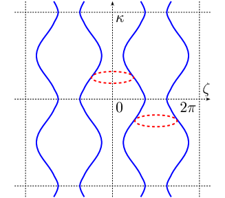
The adiabatic limit can be regarded as a semi-classical limit, and the expression $\mathcal{E}(\kappa)+W(\zeta)$ can be interpreted as a “classical” Hamiltonian corresponding to the operator (0.1). Then, from the quantum physicist point of view (see [18, 19]), a semi-classical particle should “live” near the real branches of the iso-energy curve. In our case, these curves are “extended” in momentum variable and “localized” in position variable. Therefore, they have to correspond to localized states. The decay of these states in the position variable is characterized by the complex tunneling between the real branches along the complex loops. So, the Lyapunov exponent is naturally related to the tunneling coefficients. Our results justify this heuristics.

This naturally leads to the following conjecture: in a given energy interval, if the iso-energy curve has a real branch that is an unbounded vertical curve, then, in the adiabatic limit, in this interval, the Lyapunov exponent is positive and the spectrum is singular. Note that, in [9], we have proved a dual result for the absolutely continuous spectrum: we have proved that, if, in some energy region, the branches of the real iso-energy curve are unbounded horizontal curves, then, this energy region, except for a set of exponentially small measure, is in the absolutely continuous spectrum.

1. The results

We now state our assumptions and results.

1.1. Assumptions on the potential

About the functions $V$ and $W$, we assume that

(H):

• $V$ and $W$ are periodic,

  (1.1) $$V\,(x+1)=V\,(x),\quad W\,(x+2\pi)=W\,(x),\quad x\in{\mathbb{R}};$$

• $V$ is real valued and locally square integrable;

• $W$ is real analytic in a neighborhood of ${\mathbb{R}}$, say, in the strip $\{|{\rm Im}\,z|<Y\}$;

• $W$ has exactly one maximum and one minimum in $[0,2\pi)$; they are non degenerate.

To fix notations, assume that, on the interval $[0,2\pi)$, $W$ is maximum at $0$ and minimum at $\zeta^{*}$.

In (0.1), $\varepsilon$ is a positive parameter. For each fixed $\varepsilon$, we consider (0.1) as a family of equations indexed by the parameter $z\in{\mathbb{R}}$.

Note that, if $2\pi/\varepsilon\not\in{\mathbb{Q}}$, the function $V(x-z)+W(\varepsilon x)$ is quasi-periodic in $x$, the ratio of the frequencies of $V$ and $W$ being equal to $2\pi/\varepsilon$; hence, (0.1) is an ergodic family of equations (see [15]).

1.2. The assumption on the energy region

To describe the energy regions where we study the spectral properties of the family of equations (0.1), we consider the periodic Schrödinger operator $H_{0}$ acting in $L^{2}({\mathbb{R}})$ defined by (0.2).

1.2.1. Periodic operator

The spectrum of (0.2) is absolutely continuous and consists of intervals of the real axis $[E_{1},\,E_{2}]$, $[E_{3},\,E_{4}]$, $\dots$, $[E_{2n+1},\,E_{2n+2}]$, $\dots$, such that

$$E_{1}<E_{2}\leq E_{3}<E_{4}\dots E_{2n}\leq E_{2n+1}<E_{2n+2}\leq\dots\,,$$

$$E_{n}\to+\infty,\quad n\to+\infty.$$

The points $E_{j}$,  $j=1,2,3\dots$, are the eigenvalues of the differential operator (0.2) acting on $L^{2}([0,2])$ with periodic boundary conditions. The intervals defined above are called the spectral bands, and the intervals $(E_{2},\,E_{3})$, $(E_{4},\,E_{5})$, $\dots$, $(E_{2n},\,E_{2n+1})$, $\dots$, are called the spectral gaps. If $E_{2n}<E_{2n+1}$, we say that the $n$th gap is open, and, if $[E_{2n-1},E_{2n}]$ is separated from the rest of the spectrum by open gaps, we say that the $n$-th band is isolated.

1.2.2. The “geometric” assumption

Let us now describe the energy region where we study the family of equations (0.1).

The spectral window centered at $E$ is the interval ${\mathcal{W}}(E)=E-W({\mathbb{R}})$. If $W_{+}=\max_{x\in{\mathbb{R}}}W(x)$ and $W_{-}=\min_{x\in{\mathbb{R}}}W(x)$, then, ${\mathcal{W}}(E)=[E-W_{+},E-W_{-}]$.

We assume that there exists $J\subset{\mathbb{R}}$, a compact interval such that, for all $E\in J$, the window ${\mathcal{W}}(E)$ contains exactly $m+1$ isolated bands of the periodic operator. That is, we fix two integers $n>0$ and $m$ and assume that

(A1):

the bands $[E_{2(n+j)-1},E_{2(n+j))}]$, $j=0,1,\dots m$, are isolated;

(A2):

for all $E\in J$, these bands are contained in the interior of ${\mathcal{W}}(E)$;

(A3):

for all $E\in J$, the rest of the spectrum of the periodic operator is outside ${\mathcal{W}}(E)$.

Note that energies $E$ satisfying (A1) – (A3) exist only if $W_{+}-W_{-}$, the “amplitude” of the adiabatic perturbation, is large enough; e.g., if $m=0$, such energies exist if and only if $W_{+}-W_{-}$ is larger than the size of the $n$-th spectral band, but smaller than the distance between the $(n-1)$-st and $(n+1)$-st bands.
From now on, unless stated otherwise, we assume that our assumptions on $V$ and $W$, and assumptions (A1) – (A3) are satisfied.

1.3. Iso-energy curve

Our results are formulated in terms of the iso-energy curve $\Gamma$ defined by (0.4). The iso-energy curve is $2\pi$ periodic both in the $\zeta-$ and $\kappa-$ directions (see Lemma 10.1).

1.3.1. The real branches

To describe the real branches of $\Gamma$, i.e. the connected components of the real iso-energy curve $\Gamma_{\mathbb{R}}$, we define the following collection of subintervals of $[0,2\pi]$. Consider the mapping

$$\mathcal{E}:\zeta\to E-W(\zeta).$$

It is monotonous on each of the intervals $I_{-}=[0,\zeta^{*}]$ and $I_{+}=[\zeta^{*},2\pi]$ and maps each of them onto the spectral window ${\mathcal{W}}(E)$. For $n\leq j\leq n+m$, let $\mathfrak{z}_{j}^{+}\subset I_{+}$ (resp. $\mathfrak{z}_{j}^{-}\subset I_{-}$) be the the pre-image of the $j$-th spectral band in ${\mathcal{W}}(E)$. Let $\mathcal{Z}$ be the collection of these intervals. A “period” of the real iso-energy curve is described by

Lemma 1.1.

Let $E\in J$. The set $\Gamma_{\mathbb{R}}\cap\{0\leq\kappa\leq 2\pi\}$ consists of $2(m+1)$ curves $\{\gamma(\mathfrak{z})$, $\mathfrak{z}\in\mathcal{Z}\}$.
Fix $\mathfrak{z}\in{\mathcal{Z}}$. The curve $\gamma(\mathfrak{z})$ is the graph $\{(\kappa,\zeta):\ \zeta=Z_{\mathfrak{z}}(\kappa),\ \kappa\in{\mathbb{R}}\}$ of a function $Z_{\mathfrak{z}}$ which satisfies

1. it is continuous,

2. it is $2\pi$-periodic and even in $\kappa$,

3. it is monotonous on the interval $[0,\pi]$,

4. it maps $[0,\pi]$ onto $\mathfrak{z}$.

The curves $\gamma(\mathfrak{z})$ continuously depend on $E\in J$.

Lemma 1.1 is proved in section 10.1. For $m=0$, the real iso-energy curve is shown in Fig. 2.

1.3.2. Complex loops

Now, we discuss loops, i.e. closed curves, situated on the iso-energy curve $\Gamma$ and connecting its real branches.

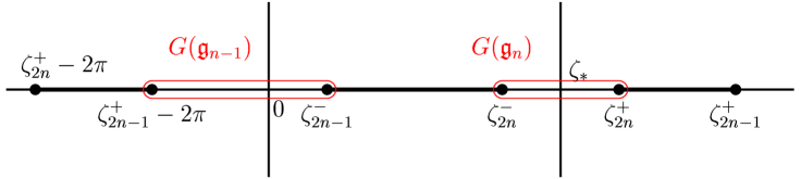
For $j=n-1,n,\dots,n+m$, let $\mathfrak{g}_{j}^{+}$ (resp. $\mathfrak{g}_{j}^{-}$) be the subinterval of $I_{+}$ (resp. $I_{-}$) that is the pre-image of the part of $j$-th spectral gap situated inside ${\mathcal{W}}(E)$. Let

$$\mathfrak{g}_{n-1}=(\mathfrak{g}_{n-1}^{+}-2\pi)\cup\mathfrak{g}_{n-1}^{-}\quad\text{and}\quad\mathfrak{g}_{n+m}=\mathfrak{g}_{n+m}^{+}\cup\mathfrak{g}_{n+m}^{-}.$$

Then, $\mathfrak{g}_{n-1}$ is an open interval containing zero, and $\mathfrak{g}_{n+m}$ is an open interval containing $\zeta^{*}$. Let $\mathcal{G}$ be the set consisting of $g_{n-1}$, $g_{n+m}$ and the intervals $g_{j}^{\pm}$ with $j=n,n+1,\dots,n+m-1$.

For $\mathfrak{g}\in{\mathcal{G}}$, let $V(\mathfrak{g})\subset{\mathbb{C}}$ be a sufficiently small complex neighborhood of the interval $\mathfrak{g}$. Let $G(\mathfrak{g})$ be a smooth closed curve that goes once around the interval $\mathfrak{g}$ in $V(\mathfrak{g})\setminus\mathfrak{g}$. In Figure 3, we depicted the curves $G(\mathfrak{g})$ when $m=0$.

In section 10.2, we show that each of the curves $G(\mathfrak{g})$ is the projection of $\hat{G}(\mathfrak{g})$, a closed curve on $\Gamma$. This curve connects the real branches projecting onto the intervals adjacent to $\mathfrak{g}$.

1.3.3. Tunneling coefficients

To $\Gamma$, we associate the tunneling coefficients

(1.2) $$t(\mathfrak{g})=e^{\textstyle-\frac{1}{2\varepsilon}S(\mathfrak{g})},\quad\mathfrak{g}\in{\mathcal{G}},$$

where $S(\mathfrak{g})$ are the tunneling actions given by

(1.3) $$S(\mathfrak{g})=i\oint_{\hat{G}(\mathfrak{g})}\kappa d\zeta,\quad\mathfrak{g}\in{\mathcal{G}}.$$

In section 10.3, we show that, for $E\in J$, each of these actions is real and non-zero. By definition, we choose the direction of the integration so that all the tunneling actions be positive.

Figure 3. The curves $G(\mathfrak{g})$ for $m=0$

1.4. Spectral results

One of the main objects of the spectral theory of quasi-periodic equations is the Lyapunov exponent, see, for example, [15]. Our main spectral result is

Theorem 1.1.

Let $J$ be an interval satisfying the assumptions (A1)-(A3) for some $n$ and $m$. Let $W$ and $V$ satisfy the hypothesis (H), and let $\varepsilon$ be irrational. Then, on the interval $J$, for sufficiently small, irrational $\varepsilon/2\pi$, the Lyapunov exponent $\Theta(E)$ for the family of equations (0.1) is positive and has the asymptotics

(1.4) $$\Theta(E)=\frac{\varepsilon}{2\pi}\sum_{\mathfrak{g}\in{\mathcal{G}}}\ln\frac{1}{t(\mathfrak{g})}+o(1)=\frac{1}{4\pi}\sum_{\mathfrak{g}\in{\mathcal{G}}}S(\mathfrak{g})+o(1).$$

Note that, this theorem implies that, if $\varepsilon$ is sufficiently small, then, the Lyapunov exponent is positive for all $E\in J$.

Recall that, if $2\pi/\varepsilon$ is irrational, then $H_{z,\varepsilon}$ is quasi-periodic. In this case, its spectrum does not depend on $z$ (see [1]); denote it by $\sigma(H_{z,\varepsilon})$. In [8], we have proved

Theorem 1.2 ([8]).

Let $\Sigma=\sigma(H_{0})+W({\mathbb{R}})=\sigma(H_{0})+[W_{-},W_{+}]$. Then, one has

• $\forall\varepsilon\geq 0$, $\sigma(H_{z,\varepsilon})\subset\Sigma$.

• for any $K\subset\Sigma$ compact, there exists $C>0$ such that for all $\varepsilon$ sufficiently small and $\forall E\in K$, one has

  $$\sigma(H_{z,\varepsilon})\cap(E-C\varepsilon^{1/2},E+C\varepsilon^{1/2})\not=\emptyset.$$

By the Ishii-Pastur-Kotani Theorem [4, 15] and Theorem 1.5 in [12], Theorems 1.1 and 1.2 imply

Corollary 1.1.

In the case of Theorem 1.1, for $\varepsilon$ sufficiently small, for all $z\in{\mathbb{R}}$, one has

$$\sigma(H_{z,\varepsilon})\cap J\not=\emptyset\quad\text{ and }\quad\sigma_{ac}(H_{z,\varepsilon})\cap J=\emptyset,$$

where $\sigma_{ac}(H_{z,\varepsilon})$ is the absolutely continuous spectrum of the family of equations (0.1).

1.5. The monodromy matrix and Lyapunov exponents

The main object of our study is the monodromy matrix for the family of equations (0.1); we define it briefly (we refer to [7, 8] for more details). The central result of the paper is its asymptotics in the adiabatic limit.

1.5.1. Definition of the monodromy matrix

Consider a consistent basis $(\psi_{1,2})$ i.e. a basis of solutions of (0.1) whose Wronskian is independent of $z$ and that are $1$-periodic in $z$ i.e. that satisfy

(1.5) $$\psi_{1,2}(x,\,z+1)=\psi_{1,2}(x,\,z),\quad\forall x,z.$$

The functions $\psi_{1,2}(x+2\pi/\varepsilon,z+2\pi/\varepsilon)$ being solutions of equation (0.1), one can write

(1.6) $$\Psi\,(x+2\pi/\varepsilon,z+2\pi/\varepsilon)=M\,(z)\,\Psi\,(x,z),$$

where

• $\displaystyle\Psi(x,z)=\begin{pmatrix}\psi_{1}(x,\,z)\\ \psi_{2}(x,z)\end{pmatrix}$,

• $M\,(z)$ is a $2\times 2$ matrix with coefficients independent of $x$.

The matrix $M$ is called the monodromy matrix associated to the consistent basis $(\psi_{1,2})$. Note that

(1.7) $$\det M\,(z)\equiv 1,\quad M\,(z+1)=M\,(z),\quad\forall z.$$

1.5.2. Monodromy equation and Lyapunov exponents

Set $h=\frac{2\pi}{\varepsilon}\,{\rm mod}\,1$. Let $M$ be the monodromy matrix associated to a consistent basis $(\psi_{1,2})$. Consider the monodromy equation

(1.8) $$F_{n+1}=M(z+nh)F_{n}\quad\quad\forall n\in{\mathbb{Z}}.$$

There are several deep relations between the monodromy equation and the family of equations (0.1) (see [9, 8]). We describe only one of them. Let $2\pi/\varepsilon$ be irrational, and let $\Theta(E)$ (resp. $\theta(E)$) be the Lyapunov exponent for (0.1) (resp. for (1.8)). One proves

Theorem 1.3 ([8]).

The Lyapunov exponents $\Theta(E)$ and $\theta(E)$ satisfy the relation

(1.9) $$\Theta(E)=\frac{\varepsilon}{2\pi}\theta(E).$$

The passage to the monodromy equation is close to the monodromization idea developed in [2] for difference equations with periodic coefficients.

1.5.3. The asymptotics of the monodromy matrix

As $W$ and $V$ are real on the real line, we construct a monodromy matrix of the form

(1.10) $$\begin{pmatrix}a(z,E)&b(z,E)\\ \overline{b(\bar{z},\bar{E})}&\overline{a(\bar{z},\bar{E})}\end{pmatrix}.$$

In the adiabatic case, the asymptotics of $a$ and $b$ have very simple, model form. We first assume that $n$ in (A1) – (A3) is odd. Then, one has

Theorem 1.4.

Let $E\in J$. There exists $Y>0$ and $V_{0}$, a neighborhood of $E_{0}$, such that, for sufficiently small $\varepsilon$, the family of equations (0.1) has a consistent basis of solutions for which the corresponding monodromy matrix $M$ is analytic in $(z,E)\in\{|{\rm Im}\,z|<Y/\varepsilon\}\times V_{0}$ and has the form (1.10). The coefficients $a$ and $b$ admit the asymptotic representations

(1.11) $$a=a_{-m}\,e^{-2\pi imz}(1+o(1)),\quad b=b_{-m}\,e^{-2\pi imz}(1+o(1)),\quad 0<{\rm Im}\,z<Y/\varepsilon,$$

and

(1.12) $$a=a_{m+1}\,e^{2\pi i(m+1)z}(1+o(1)),\quad b=b_{m+1}\,e^{2\pi i(m+1)z}(1+o(1)),\quad-Y/\varepsilon<{\rm Im}\,z<0.$$

The coefficients $a_{-m}$, $b_{-m}$, $a_{m+1}$ and $b_{m+1}$ are independent of $z$. Moreover, there exists a constant $C>1$ (independent of $\varepsilon$ and $E$) such that

(1.13) $$\begin{array}[]{c}\textstyle\frac{1}{C}\leq T\cdot|a_{j}|\leq C,\quad\quad\frac{1}{C}\leq T\cdot|b_{j}|\leq C,\quad\text{where}\quad T=T(E)=\prod_{\mathfrak{g}\in{\mathcal{G}}}t(\mathfrak{g}),\\ {}\hfil\\ E\in V_{0}\cap{\mathbb{R}},\quad j=-m,\ m+1.\end{array}$$

Pick $Y_{1}$ and $Y_{2}$ so that $0<Y_{1}<Y_{2}<Y$. There is $V=V(Y_{1},Y_{2})$, a neighborhood of $E_{0}$ such that the asymptotics of $a$ and $b$ are uniform in $(z,E)\in\{Y_{1}<|{\rm Im}\,\zeta|<Y_{2}\}\times V$.

In sections 9.1 and 9.2, we give asymptotic formulae for $a_{m+1}$, $a_{-m}$ and $b_{m+1}$, $b_{-m}$.

In the case $n$ even, one has a similar result. The only novelty is that, in this case, the formulae (1.11) and (1.12) describe the asymptotics of the coefficients of the matrix related to $M$, the monodromy matrix, by the following transformation

(1.14) $$S^{-1}(z+h)M(E,z)S(z),\quad S(z)=\begin{pmatrix}e^{i\pi z}&0\\ 0&e^{-i\pi z}\end{pmatrix}.$$

The asymptotics (1.11) and (1.12) are obtained by means of the new asymptotic method developed in [7, 10].

1.5.4. Fourier coefficients

The coefficients $a_{m+1}$, $a_{-m}$ and $b_{m+1}$, $b_{-m}$ are the leading terms of the asymptotics of the $(m+1)$-th and $(-m)$-th Fourier coefficients of the monodromy matrix coefficients. Theorem 1.4 implies that, in the strip $\{|{\rm Im}\,\zeta|<Y\}$, the leading terms of the asymptotics of the monodromy matrix are equal to the contribution of a few of its Fourier series terms.

1.5.5. The case $m=0$

When $m=0$ (and $n$ odd), Theorem 1.4 imply that, in the whole strip $\{|{\rm Im}\,z|<Y\}$, the monodromy matrix coefficients $a$ and $b$ admit the asymptotics:

(1.15) $$a=a_{0}\,(1+o(1))+a_{1}\,e^{2\pi iz}(1+o(1)),\quad b=b_{0}\,(1+o(1))+b_{1}\,e^{2\pi iz}(1+o(1)).$$

So, up to the error terms, the monodromy matrix becomes a first order trigonometric polynomial:

(1.16) $$M\sim M_{0}=\begin{pmatrix}a_{0}+a_{1}u&b_{0}+b_{1}u\\ \overline{b_{0}}+\overline{b_{1}}/u&\overline{a_{0}}+\overline{a_{1}}/u\end{pmatrix},\quad u=e^{2\pi iz},$$

with constant coefficients $a_{0}$, $a_{1}$, $b_{0}$, $b_{1}$ of order $O(1/T(E))$ (for real $E$).

We see that, for $m=0$ the monodromy equation becomes a “simple” model equation.

1.5.6. Relation to the spectral results

In this paper, we use the asymptotics of the monodromy matrix only to prove Theorem 1.1. However, we believe that these asymptotics can be used to get quite a detailed information on the spectrum of (0.1) in the adiabatic limit. Therefore, we plan to study the model equation with the matrix $M_{0}$ in a subsequent paper. In particular, it seems reasonable to believe that, under a Diophantine condition on $2\pi/\varepsilon$, the spectrum of (0.1) is pure point and the eigenvalues can be described by quantization conditions of Bohr-Sommerfeld type.

1.5.7. Organization of the paper

Section 2 is devoted to the proof of Theorem 1.1 using Theorem 1.4. In section 3, we recall some well known facts from the theory of periodic Schrödinger operators on the real line. In section 4, we recall the main construction of the asymptotic method we use to compute the monodromy matrix. In sections 5 and 6, using this method, we construct a consistent basis of solutions having a simple “standard” asymptotic behavior in the complex plane of $\zeta=\varepsilon z$. In section 7, we discuss the properties of the monodromy matrix for this basis. This is the monodromy matrix the asymptotics of which are described in Theorem 1.4. Sections 8 and 9 are devoted to the computation of the asymptotics of the monodromy matrix. In section 10, we study the geometry of the iso-energy curve $\Gamma$ and prove estimates (1.13).

2. The asymptotics for the Lyapunov exponent

In this section, we prove the asymptotics (1.4). We deduce these asymptotics from the asymptotics of the monodromy matrix coefficients described by Theorem 1.4. First, we use a statement of [8] and obtain a lower bound for the Lyapunov exponent. This statement is based on the ideas of [16] generalizing Herman’s argument [11]. Then, using the asymptotics of the coefficients of the monodromy matrix in the complex plane, we get estimates on the real line. This yields an upper bound for the Lyapunov exponent. Comparing the upper and the lower bounds, we obtain (1.4).

Recall that, for equation (1.8), the Lyapunov exponent is defined by

(2.1) $$\theta(M)=\lim_{N\to+\infty}\frac{1}{N}\log\|P_{N}(z)\|,$$

where $P_{N}$ is the matrix cocycle

$$P_{N}(z)=M(z+Nh)\cdot M(z+(N-1)h)\cdots M(z+h)\cdot M(z).$$

It is well known (see [3, 15, 16] and references therein) that, if $h$ is irrational, and $M(z)$ sufficiently regular in $z$, then the limit (2.1) exists for almost all $z$ and is independent of $z$.

2.1. The lower bound

2.1.1. Preliminaries

Let $(M(z,\varepsilon))_{0<\varepsilon<1}$ be a family of $SL(2,{\mathbb{C}})$-valued $1$-periodic functions of $z\in{\mathbb{C}}$. Let $h$ be an irrational number. One has

Proposition 2.1 ([8]).

Pick $\varepsilon_{0}>0$. Assume that there exist $y_{0}$ and $y_{1}$ satisfying the inequalities $0<y_{0}<y_{1}<\infty$ and such that, for any $\varepsilon\in(0,\varepsilon_{0})$ one has

• the function $z\to M(z,\varepsilon)$ is analytic in the strip $S=\{z\in{\mathbb{C}};\ 0\leq{\rm Im}\,z\leq y_{1}/\varepsilon\}$;

• in the strip $S_{1}=\{z\in{\mathbb{C}};\ y_{0}/\varepsilon\leq{\rm Im}\,z\leq y_{1}/\varepsilon\}\subset S$, $M(z,\varepsilon)$ admits the representation

  $$M(z,\varepsilon)=\lambda(\varepsilon)e^{i2\pi n_{0}z}\cdot\left(M_{0}(\varepsilon)+M_{1}(z,\varepsilon)\right),$$

  for some constant $\lambda(\varepsilon)$, an integer $n_{0}$ and a matrix $M_{0}(\varepsilon)$, all of them independent of $z$;

• $M_{0}(\varepsilon)=\begin{pmatrix}1&\beta(\varepsilon)\\ 0&\alpha(\varepsilon)\end{pmatrix}$;

• there exist constants $\beta>0$ and $\alpha\in(0,1)$ independent of $\varepsilon$ and such that $|\alpha(\varepsilon)|\leq\alpha$ and $|\beta(\varepsilon)|\leq\beta$;

• $\sup_{z\in S_{1}}\|M_{1}(z,\varepsilon)\|\leq m(\varepsilon)$,  $m(\varepsilon)\to 0$ as $\varepsilon\to 0$.

Then, there exit $C>0$ and $\varepsilon_{1}>0$ (both depending only on $y_{0}$, $y_{1}$, $\alpha$, $\beta$ and $m(\cdot)$) such that, if $0<\varepsilon<\varepsilon_{1}$, one has

(2.2) $$\theta(M)>\log|\lambda(\varepsilon)|-Cm(\varepsilon).$$

In [8], we have assumed that $n_{0}$ is a positive integer, but the proof remains the same for $n_{0}\in{\mathbb{Z}}$.

We use this result and Theorem 1.4 to get the lower bound for the Lyapunov exponent. In the sequel, $n$ is the index introduced in assumptions (A1) – (A3). The cases $n$ odd and $n$ even are treated separately.

2.1.2. Obtaining the lower bound for $n$ odd

In the sequel, we suppose that the assumptions of Theorem 1.4 are satisfied; we use the notations and results from this theorem without referring to it anymore. We assume that $E\in V_{0}\cap{\mathbb{R}}$.
Let $\sigma=\begin{pmatrix}0&1\\ 1&0\end{pmatrix}$. Show that the matrix $\sigma M(z)\sigma$ satisfies the assumptions of Proposition 2.1.
Fix $y_{0}$ and $y_{1}$ so that $0<y_{0}<y_{1}<Y$. The asymptotics of the monodromy matrix coefficients are uniform in $z$ in the strip $S=\{y_{0}/\varepsilon\leq{\rm Im}\,z\leq y_{1}/\varepsilon\}$ and in $E\in V_{0}$ (reducing $V_{0}$ if necessary). For $E\in V_{0}\cap{\mathbb{R}}$ and $z\in S$, formulae (1.11) and (1.12), and estimates (1.13) imply that

$$\overline{a({\overline{z}})}=\overline{a_{m+1}}e^{-2\pi i(m+1)z}(1+o(1)),\frac{\overline{b({\overline{z}})}}{\overline{a({\overline{z}})}}=c(E)\,(1+o(1)),\frac{a(z)}{\overline{a({\overline{z}})}}=o(1),\quad\frac{b}{\overline{a({\overline{z}})}}=o(1)$$

where $c(E)$ is independent of $z$ and bounded by a constant uniformly in $\varepsilon$ and $E$. So, we have

$$\sigma\,M(z)\sigma=\overline{a_{m+1}}\,e^{-2\pi i(m+1)z}\,\left[\begin{pmatrix}1&c(E)\\ 0&0\end{pmatrix}+o(1)\right].$$

We see that the matrix $\sigma M(z)\sigma$ satisfies the assumptions of Proposition 2.1.
Clearly, the Lyapunov exponents of the matrix cocycles associated to the pairs $(M,h)$ and $(\sigma M\sigma,h)$ coincide. So, Proposition 2.1 implies that $\theta(M)$, the Lyapunov exponents of the matrix cocycle associated to $(M,h)$, satisfies the estimate $\theta(M)\geq\log|a_{-m}|+o(1)$.
The Lyapunov exponent $\Theta(E)$ for equation (0.1) is related to $\theta(M)$ by Theorem 1.3. Therefore, $\Theta(E)\geq\frac{\varepsilon}{2\pi}\log|a_{-m}|+o(\varepsilon)$. Hence, (1.13) clearly implies

(2.3) $$\Theta(E)\geq\frac{\varepsilon}{2\pi}\log T^{-1}+O(\varepsilon).$$

2.1.3. The lower bound when $n$ is even

If $n$ is even, then, formulae (1.11) and (1.12) give the asymptotics of the coefficients of the matrix (1.14). Obviously, the Lyapunov exponents for the matrix cocycles generated by $M(z)$ and by $S^{-1}(z+h)M(z)S(z)$ coincide. Arguing exactly as in subsection 2.1.2, we again obtain (2.3).

2.2. The upper bound

Let us first assume that $n$ is odd. Let $E\in V_{0}\cap{\mathbb{R}}$. Fix $0<y_{0}<Y$. The asymptotics (1.11) and (1.12) and estimates (1.13) imply the following estimates for the coefficients of $M(z)$, the monodromy matrix:

(2.4) $$\begin{array}[]{c}|a|,|b|\leq C(y_{0})T^{-1}e^{2\pi my_{0}/\varepsilon},\quad{\rm Im}\,z=y_{0}/\varepsilon,\\ |a|,|b|\leq C(y_{0})T^{-1}e^{2\pi(m+1)y_{0}/\varepsilon},\quad{\rm Im}\,z=-y_{0}/\varepsilon.\end{array}$$

Here, $C(y_{0})$ is a positive constant independent of $\varepsilon$, ${\rm Re}\,z$, and $E$. The estimates are valid for sufficiently small $\varepsilon$. Recall that $M$ is analytic and $1$-periodic in $z$. Therefore, (2.4) and the Maximum Principle imply that

(2.5) $$|a|,|b|\leq 2C(y_{0})T^{-1}\exp(2\pi(m+1)y_{0}/\varepsilon),\quad z\in{\mathbb{R}}.$$

This leads to the following upper bound for the Lyapunov exponent for the matrix cocycle generated by $M$

$$\theta\leq\log T^{-1}+{\rm Const}+2\pi(m+1)y_{0}/\varepsilon$$

where ${\rm Const}$ is independent of $E$ and $\varepsilon$. In view of Theorem 1.3, we finally get

(2.6) $$\Theta(E)\leq\frac{\varepsilon}{2\pi}\log T^{-1}+\varepsilon{\rm Const}+2\pi(m+1)y_{0}.$$

The upper bound (2.6) remains true when $n$ is even as the Lyapunov exponents for the matrix cocycles generated by $M(z)$ and by $S^{-1}(z+h)M(z)S(z)$ coincide.

2.3. Completing the proof

Recall that, in (2.6), $y_{0}$ is an arbitrarily fixed positive number. So, comparing (2.3) and (2.6), we get $\displaystyle\Theta(E)=\frac{\varepsilon}{2\pi}\log T^{-1}+o(1)$. This and the formula (1.13) for $T$ imply (1.4) for all $E\in V_{0}\cap{\mathbb{R}}$.
Recall that $V_{0}\cap{\mathbb{R}}$ is an open interval containing $E_{0}\in J$. The above construction can be carried out for any $E_{0}\in J$. As the interval $J$ is compact, this completes the proof of Theorem 1.1.

3. Periodic Schrödinger operators

We now discuss the periodic Schrödinger operator (0.2) where $V$ is a $1$-periodic, real valued, $L^{2}_{loc}$-function. We collect known results needed in the present paper (see [5, 13, 14, 17, 10]).

3.1. Bloch solutions

Let $\psi$ be a solution of the equation

(3.1) $$-\frac{d^{2}}{dx^{2}}\psi\,(x)+V\,(x)\psi\,(x)=\mathcal{E}\psi\,(x),\quad x\in{\mathbb{R}},$$

satisfying the relation $\psi\,(x+1)=\lambda\,\psi\,(x)$ for all $x\in{\mathbb{R}}$ with $\lambda\in{\mathbb{C}}$ independent of $x$. Such a solution is called a Bloch solution, and the number $\lambda$ is called the Floquet multiplier. Let us discuss the analytic properties of $\mathcal{E}\mapsto\psi(\mathcal{E},x):=\psi(x)$.

As in section 1.2, we denote the spectral bands of the periodic Schrödinger equation by $[E_{1},\,E_{2}]$, $[E_{3},\,E_{4}]$, $\dots$, $[E_{2n+1},\,E_{2n+2}]$, $\dots$. Consider $\mathcal{S}_{\pm}$, two copies of the complex plane $\mathcal{E}\in{\mathbb{C}}$ cut along the spectral bands. Paste them together to get a Riemann surface with square root branch points. We denote this Riemann surface by $\mathcal{S}$.

One can construct a Bloch solution $\psi(x,\mathcal{E})$ of equation (3.1) meromorphic on $\mathcal{S}$. It is normalized by the condition $\psi(1,\mathcal{E})\equiv 1$. The poles of this solution are located in the spectral gaps. More precisely, each spectral gap contains precisely one simple pole. It is located either on $\mathcal{S}_{+}$ or on $\mathcal{S}_{-}$. The position of the pole is independent of $x$.

For $\mathcal{E}\in\mathcal{S}$, we denote by $\hat{\mathcal{E}}$ the point on $\mathcal{S}$ having the same projection on ${\mathbb{C}}$ as $\mathcal{E}$. We let

$$\hat{\psi}(x,\mathcal{E})=\psi(x,\hat{\mathcal{E}}),\quad\mathcal{E}\in\mathcal{S}.$$

The function $\hat{\psi}(x,\mathcal{E})$ is another Bloch solution of (3.1). Except at the edges of the spectrum (i.e. the branch points of $\mathcal{S}$), the functions $\psi$ and $\hat{\psi}$ are linearly independent solutions of (3.1). In the spectral gaps, $\psi$ and $\hat{\psi}$ are real valued functions of $x$, and, on the spectral bands, they differ only by complex conjugation.

3.2. The Bloch quasi-momentum

Consider the Bloch solution $\psi(x,\mathcal{E})$. The corresponding Floquet multiplier $\lambda\,(\mathcal{E})$ is analytic on $\mathcal{S}$. Represent it in the form $\lambda(\mathcal{E})=\exp(ik(\mathcal{E}))$. The function $k(\mathcal{E})$ is the Bloch quasi-momentum.

The Bloch quasi-momentum is an analytic multi-valued function of $\mathcal{E}$. It has the same branch points as $\psi(x,\mathcal{E})$.

Let $D$ be a simply connected domain containing no branch point of the Bloch quasi-momentum. In $D$, one can fix an analytic single-valued branch of $k$, say $k_{0}$. All the other single-valued branches of $k$ that are analytic in $D$ are related to $k_{0}$ by the formulae

(3.2) $$k_{\pm,l}(\mathcal{E})=\pm k_{0}(\mathcal{E})+2\pi l,\quad l\in{\mathbb{Z}}.$$

Consider ${\mathbb{C}}_{+}$ the upper half plane of the complex plane. On ${\mathbb{C}}_{+}$, one can fix a single valued analytic branch of the quasi-momentum continuous up to the real line. It can be fixed uniquely by the condition $-ik(\mathcal{E}+i0)>0$ as $\mathcal{E}<E_{1}$. We call this branch the main branch of the Bloch quasi-momentum and denote it by $k_{p}$.

The function $k_{p}$ conformally maps ${\mathbb{C}}_{+}$ onto the first quadrant of the complex plane cut at compact vertical slits starting at the points $\pi l$, $l\in{\mathbb{N}}$. It is monotonically increasing along the spectral zones so that $[E_{2n-1},E_{2n}]$, the $n$-th spectral band, is mapped on the interval $[\pi(n-1),\pi n]$. Along any open gap, ${\rm Re}\,k_{p}(\mathcal{E}+i0)$ is constant, and ${\rm Im}\,k_{p}(\mathcal{E}+i0)$ is positive and has only one non-degenerate maximum.

All the branch point of $k_{p}$ are of square root type. Let $E_{l}$ be a branch point. In a sufficiently small neighborhood of $E_{l}$, the function $k_{p}$ is analytic in $\sqrt{\mathcal{E}-E_{l}}$, and

(3.3) $$k_{p}(\mathcal{E})-k_{p}(E_{l})=c_{l}\sqrt{\mathcal{E}-E_{l}}+O(\mathcal{E}-E_{l}),\quad c_{l}\not=0.$$

Finally, we note that the main branch can be analytically continued on the complex plane cut only along the spectral gaps of the periodic operator.

3.3. A meromorphic function

Here, we discuss a function playing an important role in the adiabatic constructions.

In [10], we have seen that, on $\mathcal{S}$, there is a meromorphic function $\omega$ having the following properties:

• the differential $\Omega=\omega\,d\mathcal{E}$ is meromorphic; its poles are the points of $P\cup Q$, where $P$ is the set of poles of $\psi(x,\mathcal{E})$, and $Q$ is the set of points where $k^{\prime}(\mathcal{E})=0$.

• all the poles of $\Omega$ are simple;

• ${\rm res}\,_{p}\Omega=1$,  $\forall p\in P\setminus Q$,   ${\rm res}\,_{q}\Omega=-1/2$,  $\forall q\in Q\setminus P$,   ${\rm res}\,_{r}\Omega=1/2$,  $\forall r\in P\cap Q$.

• if $\mathcal{E}\in\mathcal{S}$ projects into a gap, then $\omega(\mathcal{E})\in{\mathbb{R}}$;

• if $\mathcal{E}\in\mathcal{S}$ projects inside a band, then $\overline{\omega(\mathcal{E})}=\omega(\hat{\mathcal{E}})$.

4. The complex WKB method for adiabatic problems

In this section, following [7, 10], we briefly describe the complex WKB method for adiabatically perturbed periodic Schrödinger equations

(4.1) $$-\frac{d^{2}}{dx^{2}}\psi(x)+(V(x)+W(\varepsilon x+\zeta))\psi(x)=E\psi(x),\quad x\in{\mathbb{R}}.$$

Here, $V$ is $1$-periodic and $\varepsilon$ is a small positive parameter; one assumes that $V\in L_{\rm loc}^{2}$ and that $W$ is analytic in ${\mathcal{D}}(W)$, a neighborhood of the real line ($W$ is not necessarily periodic).

The parameter $\zeta$ is an auxiliary parameter used to decouple the “slow variable” $\xi=\varepsilon x$ and the “fast variable” $x$. The idea of the method is to study solutions of (4.1) on the complex plane of $\zeta$ and, then to recover information on their behavior in $x\in{\mathbb{R}}$. Therefore, one studies solutions satisfying the condition:

(4.2) $$\psi(x+1,\zeta)=\psi(x,\zeta+\varepsilon)\quad\forall\zeta.$$

On the complex plane of $\zeta$, there are certain domains on which one can construct such solutions that, moreover, have simple asymptotic behavior.

4.1. Standard behavior of solutions

We first define two analytic objects central to the complex WKB method, the complex momentum and the canonical Bloch solutions. Then, we describe the standard behavior of the solutions studied in the framework of the complex WKB method.

4.1.1. The complex momentum

The complex momentum $\kappa$ is the main analytic object of the complex WKB method. For $\zeta\in\mathcal{D}(W)$, the domain of analyticity of the function $W$, it is defined by the formula

(4.3) $$\kappa(\zeta)=k(\mathcal{E}(\zeta)),\quad\mathcal{E}(\zeta)=E-W(\zeta),$$

Here, $k$ is the Bloch quasi-momentum of (0.2). Relation (4.3) “translates” properties of $k$ into properties of $\kappa$. Hence, $\kappa$ is a multi-valued analytic function, and that its branch points are related to the branch points of the quasi-momentum by the relations

(4.4) $$E_{l}+W(\zeta)=E,\quad l=1,2,3\dots$$

Let $\zeta_{0}$ be a branch point of $\kappa$. If $W^{\prime}(\zeta_{0})\neq 0$, then $\zeta_{0}$ is a branch point of square root type.

If $D\subset\mathcal{D}(W)$ is a simply connected set containing no branch points of $\kappa$, we call it regular. Let $\kappa_{p}$ be a branch of the complex momentum analytic in a regular domain $D$. All the other branches analytic in $D$ are described by the formulae:

(4.5) $$\kappa_{m}^{\pm}=\pm\kappa_{p}+2\pi m,$$

where $\pm$ and $m\in{\mathbb{Z}}$ are indexing the branches.

4.1.2. Canonical Bloch solutions

To describe the asymptotic formulae of the complex WKB method, one needs Bloch solutions to the equation

(4.6) $$-\frac{d^{2}}{dx^{2}}\psi(x)+V(x)\psi(x)={\mathcal{E}}(\zeta)\psi(x),\quad{\mathcal{E}}(\zeta)=E-W(\zeta),\quad x\in{\mathbb{R}},$$

that, moreover, are analytic in $\zeta$ on a given regular domain.

Pick $\zeta_{0}$ a regular point. Let $\mathcal{E}_{0}=\mathcal{E}(\zeta_{0})$. Assume that $\mathcal{E}_{0}\not\in P\cup Q$. Let $U_{0}$ be a sufficiently small neighborhood of ${\mathcal{E}}_{0}$, and let $V_{0}$ be a neighborhood of $\zeta_{0}$ such that ${\mathcal{E}}(V_{0})\subset U_{0}$. In $U_{0}$, we fix a branch of the function $\sqrt{k^{\prime}(\mathcal{E})}$ and consider $\psi_{\pm}(x,\mathcal{E})$, two branches of the Bloch solution $\psi(x,\mathcal{E})$, and $\Omega_{\pm}$, the corresponding branches of $\Omega$. Put

(4.7) $$\Psi_{\pm}(x,\zeta)=q(\mathcal{E})\,e^{\int_{\mathcal{E}_{0}}^{\mathcal{E}}\Omega_{\pm}}\psi_{\pm}(x,\mathcal{E}),\quad q(\mathcal{E})=\sqrt{k^{\prime}(\mathcal{E})},\quad\mathcal{E}=\mathcal{E}(\zeta).$$

The functions $\Psi_{\pm}$ are called the canonical Bloch solutions normalized at the point $\zeta_{0}$.

The properties of the differential $\Omega$ imply that the solutions $\Psi_{\pm}$ can be analytically continued from $V_{0}$ to any regular domain $D$ containing $V_{0}$.
One has (see [10])

(4.8) $$w(\Psi_{+}(\cdot,\zeta),\Psi_{-}(\cdot,\zeta))=w(\Psi_{+}(\cdot,\zeta_{0}),\Psi_{-}(\cdot,\zeta_{0}))=k^{\prime}(\mathcal{E}_{0})w(\psi_{+}(x,\mathcal{E}_{0}),\psi_{-}(x,\mathcal{E}_{0}))$$

As $\mathcal{E}_{0}\not\in Q\cup\{E_{l}\}$, the Wronskian $w(\Psi_{+}(\cdot,\zeta),\Psi_{-}(\cdot,\zeta))$ is non-zero.

4.2. Solutions having standard asymptotic behavior

Fix $E=E_{0}$. Let $D$ be a regular domain. Fix $\zeta_{0}\in D$ so that $\mathcal{E}(\zeta_{0})\not\in P\cup Q$. Let $\kappa$ be a branch of the complex momentum continuous in $D$, and let $\Psi_{\pm}$ be the canonical Bloch solutions defined on $D$, normalized at $\zeta_{0}$ and indexed so that $\kappa$ be the quasi-momentum for $\Psi_{+}$.

Definition 4.1.

Let $\sigma$ be either $+$ or $-$. We say that, in $D$, a solution $f$ has standard behavior (or standard asymptotics) $f\sim\exp(\sigma\frac{i}{\varepsilon}\int^{\zeta}\kappa\,d\zeta)\cdot\Psi_{\sigma}$ if

• there exists $V_{0}$, a complex neighborhood of $E_{0}$, and $X>0$ such that $f$ is defined and satisfies (4.1) and (4.2) for any $(x,\zeta,E)\in[-X,X]\times D\times V_{0}$;

• $f$ is analytic in $\zeta\in D$ and in $E\in V_{0}$;

• for any $K$, a compact subset of $D$, there is $V\subset V_{0}$, a neighborhood of $E_{0}$, such that, for $(x,\zeta,E)\in[-X,X]\times K\times V$, $f$ has the uniform asymptotic

  (4.9) $$f=e^{\textstyle\sigma\,\frac{i}{\varepsilon}\int^{\zeta}\kappa\,d\zeta}\,(\Psi_{\sigma}+o\,(1)),\quad\text{as}\quad\varepsilon\to 0,$$

• this asymptotic can be differentiated once in $x$ without loosing its uniformity properties.

4.3. Canonical domains

Canonical domains are important examples of domains where one can construct solutions with standard asymptotic behavior. They are defined using canonical lines.

4.3.1. Canonical lines

A curve is called vertical if it is connected, piecewise $C^{1}$, and if it intersects the lines $\{{\rm Im}\,\zeta={\rm Const}\}$ at non-zero angles $\theta$,  $0<\theta<\pi$. Vertical curves are naturally parameterized by ${\rm Im}\,\zeta$.

Let $\gamma$ be a regular curve. On $\gamma$, fix $\kappa$, a continuous branch of the complex momentum.

Definition 4.2.

The curve $\gamma$ is canonical if it is vertical and such that, along $\gamma$,

1. ${\rm Im}\,\int^{\zeta}\kappa d\zeta$ is strictly monotonously increasing with ${\rm Im}\,\zeta$,

2. ${\rm Im}\,\int^{\zeta}(\kappa-\pi)d\zeta$ is strictly monotonously decreasing with ${\rm Im}\,\zeta$.

Note that canonical lines are stable under small $\mathcal{C}^{1}$-perturbations.

4.3.2. Canonical domains

Let $K$ be a regular domain. On $K$, fix a continuous branch of the complex momentum, say $\kappa$. The domain $K$ is called canonical if it is the union of curves canonical with respect to $\kappa$ and connecting two points $\zeta_{1}$ and $\zeta_{2}$ located on $\partial K$.

One has

Theorem 4.1 ([10]).

Let $K$ be a bounded domain canonical with respect to $\kappa$. For sufficiently small positive $\varepsilon$, there exists $(f_{\pm})$, two solutions of (4.1), having the standard behavior in $K$:

$$f_{\pm}\sim\exp\left(\pm\frac{i}{\varepsilon}\int_{\zeta_{0}}^{\zeta}\kappa d\zeta\right)\Psi_{\pm}.$$

For any fixed $x\in{\mathbb{R}}$, the functions $f_{\pm}(x,\zeta)$ are analytic in $\zeta$ in the smallest strip $\{Y_{1}<{\rm Im}\,\zeta<Y_{2}\}$ containing $K$.

One easily calculates the Wronskian of the solutions $f_{\pm}(x,\zeta)$ to get

(4.10) $$w(f_{+},f_{-})=w(\Psi_{+},\Psi_{-})+o(1).$$

By (4.8), for $\zeta$ in any fixed compact subset of $K$ and $\varepsilon$ sufficiently small, the solutions $f_{\pm}$ are linearly independent.

4.4. The strategy of the WKB method

Our strategy to apply the complex WKB method is explained in great detail in [10]; we recall it briefly. First, we find a canonical line. Roughly, we build it out of segments of some “elementary” curves described in section 4.6. Then, we find a “local” canonical domain $K$ “enclosing” this line, see section 4.5. For this domain, we construct the solutions $f_{\pm}$ using Theorem 4.1.

Second, we describe the asymptotic behavior of $f_{\pm}$ outside the domain $K$. Therefore, we use three general principles presented in section 4.7.

Having investigated the behavior of $f_{\pm}$ for $-X\leq x\leq X$ and a sufficiently large set of $\zeta$, we recover the behavior of $f_{\pm}$ on the real line of $x$ by means of condition (4.2).

Below, we assume that $D$ is a regular domain, and that $\kappa$ is a branch of the complex momentum analytic in $D$. A segment of a curve is a connected, compact subset of that curve.

4.5. Local canonical domains

Let $\gamma\subset D$ be a canonical line (with respect to $\kappa$). Denote its ends by $\zeta_{1}$ and $\zeta_{2}$. Let a domain $K\subset D$ be a canonical domain corresponding to the triple $\kappa$, $\zeta_{1}$ and $\zeta_{2}$. If $\gamma\in K$, then, $K$ is called a canonical domain enclosing $\gamma$. One has

Lemma 4.1 ([8]).

One can construct a canonical domain enclosing any given canonical curve.

Canonical domains whose existence is a consequence of this lemma are called local.

4.6. Pre-canonical lines

To construct a local canonical domain we need a canonical line. To construct such a line, we first build a pre-canonical line made of some “elementary” curves.

Let $\gamma\subset D$ be a vertical curve. We call $\gamma$ pre-canonical if it is a finite union of segments of canonical lines and/or lines of Stokes type i.e. the level curves of the harmonic functions $\zeta\mapsto{\rm Im}\,\int^{\zeta}\kappa d\zeta$ or $\zeta\mapsto{\rm Im}\,\int^{\zeta}(\kappa-\pi)d\zeta$. One has

Proposition 4.1 ([8]).

Let $\gamma$ be a pre-canonical curve. Denote the ends of $\gamma$ by $\zeta_{a}$ and $\zeta_{b}$.
For $V\subset D$, a neighborhood of $\gamma$ and $V_{a}\subset D$, a neighborhood of $\zeta_{a}$, there exists a canonical line $\gamma\subset V$ connecting the point $\zeta_{b}$ to a point in $V_{a}$.

When constructing pre-canonical lines, one uses lines of Stokes type. To analyze them, one uses

Lemma 4.2.

The lines of Stokes type of the family ${\rm Im}\,\int^{\zeta}\kappa\,d\zeta={\rm Const}$ are tangent to the vector field $\overline{\kappa(\zeta)}$; those of the family ${\rm Im}\,\int^{\zeta}(\kappa-\pi)\,d\zeta={\rm Const}$ are tangent to the vector field $\overline{\kappa(\zeta)}-\pi$.

4.7. Tools for computing global asymptotics

A set is said to be constant if it is independent of $\varepsilon$.

4.7.1. The Rectangle Lemma: asymptotics of increasing solutions

The Rectangle Lemma roughly says that a solution $f$ preserve the standard behavior along a line ${\rm Im}\,\zeta={\rm Const}$ as long as the leading term of the standard asymptotics increases.

Fix $\eta_{m}<\eta_{M}$. Define $S=\{\zeta\in{\mathbb{C}}:\ \eta_{m}\leq{\rm Im}\,\zeta\leq\eta_{M}\}$. Let $\gamma_{1}$ and $\gamma_{2}$ be two vertical lines such that $\gamma_{1}\cap\gamma_{2}=\emptyset$. Assume that both lines intersect the strip $S$ at the lines ${\rm Im}\,\zeta=\eta_{m}$ and ${\rm Im}\,\zeta=\eta_{M}$, and that $\gamma_{1}$ is situated to the left of $\gamma_{2}$.
Consider the compact $R$ bounded by $\gamma_{1}$, $\gamma_{2}$ and the boundaries of $S$. Let $D$=$R\setminus(\gamma_{1}\cup\gamma_{2})$. One has

Lemma 4.3 (The Rectangle Lemma [9]).

Assume that the “rectangle” $R$ is contained in a regular domain. Let $f$ be a solution to (4.1) satisfying (4.2). Then, for sufficiently small $\varepsilon$, one has

1:

If ${\rm Im}\,\kappa<0$ in $D$, and if $f$ has standard behavior $f\sim e^{\frac{i}{\varepsilon}\int_{\zeta_{0}}^{\zeta}\kappa d\zeta}\Psi_{+}$ in a neighborhood of $\gamma_{1}$, then, it has standard behavior in a constant domain containing the “rectangle” $R$.

2:

If ${\rm Im}\,\kappa>0$ in $D$, and if $f$ has standard behavior $f\sim e^{\frac{i}{\varepsilon}\int_{\zeta_{0}}^{\zeta}\kappa d\zeta}\Psi_{+}$ in a neighborhood of $\gamma_{2}$, then, it has the standard behavior in a constant domain containing the “rectangle” $R$.

Lemma 4.3 was proved in [9] where one can find more details and references.

4.7.2. The Adjacent Canonical Domain Principle

This principle complements the Rectangle Lemma; it allows us to obtain the asymptotics of decreasing solutions.

Let $\gamma$ be a vertical curve. Let $S$ be the minimal strip of the form $\{C_{1}\leq{\rm Im}\,\zeta\leq C_{2}\}$ containing $\gamma$. Let $U\subset S$ be a regular domain such that $\gamma\subset\partial U$. We say that $U$ is adjacent to $\gamma$. One has

Proposition 4.2 (The Adjacent Canonical Domain Principle [9]).

Let $\gamma$ be a canonical line. Assume that $f$, a solution to (4.1) satisfying (4.2) has standard behavior in a domain adjacent to $\gamma$. Then, $f$ has the standard behavior in any bounded canonical domain enclosing $\gamma$.

4.7.3. Adjacent canonical domains

To apply the Adjacent Canonical Domain Principle, one needs to describe canonical domains enclosing a given canonical line. It can be quite difficult to find a “maximal” canonical domain enclosing a given canonical line. In practice, one uses “simple” canonical domains described in

Lemma 4.4 (The Trapezium Lemma [10]).

Let $\gamma_{0}$ be a canonical line.

Let $U$ be a domain adjacent to $\gamma$, a canonical line containing $\gamma_{0}$ as an internal segment. Assume that, in $U$, ${\rm Im}\,\kappa\neq 0$. Let $\sigma_{u}$ (resp. $\sigma_{d}$) be the line of Stokes type beginning at the upper (resp. lower) end of $\gamma_{0}$ and going in $U$ downward (resp. upward) from this point.
One has:

Trapezium case:

Let $T\subset U$ be a regular domain bounded by $\sigma_{u}$, $\sigma_{d}$, $\gamma_{0}$ and $\tilde{\gamma}$, one more canonical line not intersecting $\gamma_{0}$. Then, $T$ is part of a canonical domain enclosing $\gamma_{0}$.

Triangle case:

Assume that $\sigma_{u}$ intersects $\sigma_{d}$. Let $T\subset U$ be a regular domain bounded by $\sigma_{u}$, $\sigma_{d}$ and line $\gamma_{0}$. Then, $T$ is part of a canonical domain enclosing $\gamma_{0}$.

There always exists a canonical line containing $\gamma_{0}$; moreover, if ${\rm Im}\,\kappa\neq 0$ in $U$, then, the lines $\sigma_{d}$ and $\sigma_{u}$ described in the Trapezium Lemma always exist (see Lemma 5.3 from [10]).

4.7.4. The Stokes Lemma

The domains where one justifies the standard behavior using the Adjacent Canonical Domain Principle are often bounded by Stokes lines (see definition below) beginning at branch points of the complex momentum. The Stokes Lemma allows us to justify the standard behavior beyond these lines by “going around” the branch points.

Notations and assumptions. Assume that $\zeta_{0}$ is a branch point of the complex momentum such that $W^{\prime}(\zeta_{0})\neq 0$.

Definition 4.3.

The Stokes lines starting at $\zeta_{0}$ are the
curves $\gamma$ defined by

$$\hskip-170.71652pt{\rm Im}\,\int_{\zeta_{0}}^{\zeta}(\kappa(\zeta)-\kappa(\zeta_{0}))d\zeta=0,\quad\zeta\in\gamma.$$

The angles between the Stokes lines at $\zeta_{0}$ are equal to $2\pi/3$. We denote them by $\sigma_{1}$, $\sigma_{2}$ and $\sigma_{3}$ so that $\sigma_{1}$ is vertical at $\zeta_{0}$ (see Fig. 4).

Let $\tilde{\sigma}_{1}$ be a (compact) segment of $\sigma_{1}$ which begins at $\zeta_{0}$, is vertical and contains only one branch point, i.e. the point $\zeta_{0}$. Let $V$ be a neighborhood of $\tilde{\sigma}_{1}$. Assume that $V$ is so small that the Stokes lines $\sigma_{1}$, $\sigma_{2}$ and $\sigma_{3}$ divide it into three sectors. We denote them by $S_{1}$, $S_{2}$ and $S_{3}$ so that $S_{1}$ be situated between $\sigma_{1}$ and $\sigma_{2}$, and the sector $S_{2}$ be between $\sigma_{2}$ and $\sigma_{3}$ (see Fig. 4).

The statement. In [10], we have proved

Lemma 4.5 (Stokes Lemma).

Let $V$ be sufficiently small.

Figure 4. The Stokes lines in a neighborhood of a branch point

Let $f$ be a solution to (4.1) satisfying (4.2) that has standard behavior $f\sim e^{\frac{i}{\varepsilon}\int^{\zeta}\kappa d\zeta}\Psi_{+}$ inside the sector $S_{1}\cup\sigma_{2}\cup S_{2}$ of $V$. Moreover, assume that, in $S_{1}$ near $\sigma_{1}$, one has ${\rm Im}\,\kappa(\zeta)>0$ if $S_{1}$ is to the left of $\sigma_{1}$ and ${\rm Im}\,\kappa(\zeta)>0$ otherwise.
Then, $f$ has standard behavior inside $V\setminus\sigma_{1}$, the leading term of the asymptotics being obtained by analytic continuation from $S_{1}\cup\sigma_{2}\cup S_{2}$ into $V^{\prime}$.

Comments and details on this lemma can be found in [10].

5. A consistent solution

We now begin the construction of the consistent basis the monodromy matrix of which we compute. Recall that $V$ and $W$ satisfy the hypothesis (H), and fix $E=E_{0}\in J$, an interval satisfying the hypothesis (A1) – (A3),

In the present section, by means of the complex WKB method, we construct and study $f$ a solution of (0.1) satisfying the consistency condition (1.5).

To use the complex WKB method, we rewrite (0.1) in terms of the variables

(5.1) $$x:=x-z,\quad\text{and}\quad\zeta=\varepsilon z.$$

It then takes the form (4.1). In the new variables, the consistency condition (1.5) becomes (4.2)

We first describe the complex momentum and Stokes lines. Then, we construct a local canonical domain, hence, a consistent solution to (4.1) by Theorem 4.1. Finally, using the continuation tools, we describe global asymptotics of this solution.

5.1. The complex momentum

We begin with the analysis of the mapping $\mathcal{E}:\zeta\to E-W(\zeta)$.

5.1.1. The set $W^{-1}({\mathbb{R}})$

As $E\in{\mathbb{R}}$, $\mathcal{E}^{-1}({\mathbb{R}})$ coincides with $W^{-1}({\mathbb{R}})$.

The set $W^{-1}({\mathbb{R}})$ is $2\pi$-periodic. It consists of the real line and of complex branches (curves) symmetric with respect to the real line. There are complex branches separated from the real line, and complex branches beginning at the real extrema of $W$. These do not return to the real line.

Consider an extremum of $W$ on the real line, say $\zeta_{0}$. By assumption (H), it is non-degenerate. This implies that, near $\zeta_{0}$, the set $W^{-1}({\mathbb{R}})$ consists of a real segment, and of a “complex” curve symmetric with respect to the real axis, intersecting the real axis at $\zeta_{0}$ only. This curve is orthogonal to the real line at $\zeta_{0}$.

For $Y>0$, we let $\mathcal{S}_{Y}=\{-Y\leq{\rm Im}\,\zeta\leq Y\}$. We assume that $Y$ is so small that

• $S_{Y}$ is contained in the domain of analyticity of $W$;

• the set $W^{-1}({\mathbb{R}})\cap{\mathcal{S}}_{Y}$ consists of the real line and of the complex lines passing through the real extrema of $W$;

For such $Y$, and if $m=0$, the set $W^{-1}({\mathbb{R}})\cap{\mathcal{S}}_{Y}$ is shown in Fig. 5.

5.1.2. Branch points

The branch points of the complex momentum are related to the branch points of the Bloch quasi-momentum by equation (4.4). So, they lie on $W^{-1}({\mathbb{R}})$, and form a $2\pi$-periodic set.

Consider the branch points situated in the interval $[0,2\pi)$ of the real line. Recall that, by assumption, the function $\zeta\mapsto W(\zeta)$ has two extrema in $[0,2\pi]$: a maximum at $\zeta=0$ and a minimum at $\zeta^{*}$, $0<\zeta^{*}<2\pi$. The mapping $\mathcal{E}$ is monotonous on each of the intervals $I_{-}=[0,\zeta_{*}]$ and $I_{+}=[\zeta^{*},2\pi]$ and maps both $I_{\pm}$ onto the interval $[E-W_{+},E-W_{-}]$. Under the hypotheses (A1) – (A3), the interval $[E-W_{+},E-W_{-}]$ contains $2m+2$ branch points of the Bloch quasi-momentum, namely the points $E_{j}$ for $j=2n-1,2n\dots 2(n+m)$. Therefore, on $[0,2\pi]$, one has $4m+4$ branch points of the complex momentum $\zeta_{j}^{\pm}$,  $j=2n-1,2n,\dots 2(n+m)$, such that $\zeta_{j}^{\pm}\in I_{\pm}$ and $\mathcal{E}(\zeta_{j}^{\pm})=E_{j}$. They satisfy the inequalities

(5.2) $$0<\zeta_{2n-1}^{-}<\zeta_{2n}^{-}<\dots<\zeta_{2(n+m)}^{-}<\zeta^{\ast}<\zeta_{2(n+m)}^{+}<\zeta_{2(n+m)-1}^{+}<\dots<\zeta_{2n-1}^{+}<2\pi.$$

The complex branch points all lie on $W^{-1}({\mathbb{R}})$. Reducing $Y$, at no loss of generality, we from now on assume that the strip ${\mathcal{S}}_{Y}$ contains only the real branch points of the complex momentum.

5.1.3. The sets $Z$ and $G$

Consider the gaps and bands of the periodic operator (0.2). Let $Z$ and $G$ respectively be the pre-image (with respect to $\mathcal{E}$) of the bands and the pre-image of the gaps. Clearly, $Z\cup G=W^{-1}({\mathbb{R}})$, and $Z\cap G=\emptyset$. Connected components of $Z$ and $G$ are separated by branch points of the complex momentum.

Figure 5. The branch points when $m=0$

The set $Z$ is $2\pi$-periodic. Consider the part of $Z$ situated in the interval $[0,2\pi]$. Consider $\mathcal{Z}$, the collection of subintervals of $[0,2\pi]$ defined in section 1.3.1. One has

(5.3) $$\hskip-85.35826pt\mathfrak{z}_{j}^{-}=[\zeta_{2j-1}^{-},\zeta_{2j}^{-}],\quad\mathfrak{z}_{j}^{+}=[\zeta_{2j}^{+},\zeta_{2j-1}^{+}],\quad j=n,n+1,\dots n+m.$$

Under our assumptions on $Y$, the set $Z\cap S_{Y}$ consists of the intervals of $\mathcal{Z}$ and their $2\pi$-translates.

Define the finite collection of intervals $\mathcal{G}$ as in section 1.3.2. One has

(5.4) $$\begin{split}\hskip-85.35826pt\mathfrak{g}_{j}^{-}=(\zeta_{2j}^{-},\zeta_{2j+1}^{-}),&\quad\mathfrak{g}_{j}^{+}=(\zeta_{2j+1}^{+},\zeta_{2j}^{+}),\quad j=n,n+1,\dots n+m-1,\\ \hskip-85.35826pt\mathfrak{g}_{n-1}&=(\zeta_{2n-1}^{+}-2\pi,\zeta_{2n-1}^{-}),\quad\mathfrak{g}_{n+m}=(\zeta_{2(n+m)}^{-},\zeta_{2(n+m)}^{+}),\end{split}$$

The set $G\cap S_{Y}$ consists of the following connected components:

• the intervals $\mathfrak{g}_{j}^{\pm}$, $j=n,\dots n+m-1$;

• the connected component containing $\zeta=0$ (it is the union of the interval $\mathfrak{g}_{n-1}$ and the complex branch of $W^{-1}({\mathbb{R}})\cap S_{Y}$ passing through $0$);

• the connected component containing $\zeta=\zeta^{*}$ (it is the union of the interval $\mathfrak{g}_{n+m}$ and the complex branch of $W^{-1}({\mathbb{R}})\cap S_{Y}$ passing through $\zeta^{*}$);

• all the $2\pi$-translates of the curves mentioned above.

5.1.4. The main branch of the complex momentum

Introduce the main branch of the complex momentum. In the strip $\{0<{\rm Im}\,\zeta<Y\}$, consider the domain $D_{p}$ between the complex branches of $W^{-1}({\mathbb{R}})$ beginning at $0$ and at $\zeta^{*}$. It is regular and ${\mathcal{E}}=E-W(\zeta)$ conformally maps it onto a domain in the upper half of the complex plane. We define the main branch of $\kappa$ by the formula

(5.5) $$\kappa_{p}(\zeta)=k_{p}(E-W(\zeta)),\quad\zeta\in D_{p},$$

where $k_{p}$ is the main branch of the Bloch quasi-momentum of the periodic operator (0.2) (see section 3.2). Clearly, ${\rm Im}\,\kappa_{p}>0$ in $D_{p}$ and the function $\kappa_{p}$ is continuous up to the boundary of $D_{p}$. Its behavior at the boundary of $D_{p}$ reflects the behavior of $k_{p}$ along the real line. In particular, for each $j=n,n+1\dots,n+m$, it is monotonously increasing on $\mathfrak{z}_{j}^{-}$ and maps it onto $[\pi(j-1),\pi j]$.

5.1.5. The Stokes lines

Consider the Stokes lines beginning at $\zeta_{2n-1}^{-}$ and $\zeta_{2n}^{-}$. As $\kappa_{p}$ is real on $\mathfrak{z}_{n}^{-}=[\zeta_{2n-1}^{-},\zeta_{2n}^{-}]$, this interval is a Stokes line both for $\zeta_{2n-1}^{-}$ and $\zeta_{2n}^{-}$. Pick one of these points. As $W^{\prime}\neq 0$ at this point, the angles between the Stokes lines beginning at it are equal to $2\pi/3$. So, one of the Stokes lines is going upwards, one is going downwards. These two Stokes lines are symmetric with respect to the real line.

Denote by $\sigma_{1}$ the Stokes line starting from $\zeta_{2n-1}^{-}$ going downwards, and denote by $\sigma_{2}$ be the Stokes line beginning at $\zeta_{2n}^{-}$ and going upwards (see Fig. 6).

The lines $\sigma_{1}$ and $\sigma_{2}$ are vertical in $S_{Y}$. Indeed, a Stokes line stays vertical as long as ${\rm Im}\,\kappa\neq 0$; the imaginary part of the complex momentum vanishes only on $Z$, and $Z\cap S_{Y}\subset{\mathbb{R}}$.

Reducing $Y$ if necessary, we can assume that $\sigma_{1}$ and $\sigma_{2}$ intersect the boundaries of $S_{Y}$.

5.2. Local construction of the solution $f$

We construct $f$ on a local canonical domain. To construct a local canonical domain, we need a canonical line. To find a canonical line, we first build a pre-canonical line.

5.2.1. Pre-canonical line

Consider the curve $\beta$ which is the union of the Stokes lines $\sigma_{1}$, $[\zeta_{2n-1}^{-},\zeta_{2n}^{-}]$ and $\sigma_{2}$. Let us construct $\alpha$, a pre-canonical line close to the line $\beta$. It goes around the branch points of the complex momentum as shown in Fig. 7.
When speaking of $\kappa_{p}$ along $\alpha$, we mean the branch of the complex momentum obtained of $\kappa_{p}$ by analytic continuation along this line (the analytic continuation can be done using formula (4.3)).

Actually, the line $\alpha$ will be pre-canonical with respect to the branch of the complex momentum related to $\kappa_{p}$ by the formula:

(5.6) $$\kappa=\left\{\begin{array}[]{ll}\kappa_{p}-\pi(n-1)&\quad\text{if \ }n\text{\ is \ odd}\\ \pi n-\kappa_{p}&\quad\text{if \ }n\text{\ is \ even}\end{array}\right.\quad\quad\zeta\in D_{p}.$$

In view of (4.5), $\kappa$ is indeed a branch of the complex momentum. We prove

Lemma 5.1.

Fix $\delta>0$. In the $\delta$-neighborhood of $\beta$, to the left of $\beta$, there exists $\alpha$, a line pre-canonical with respect to the branch $\kappa$ such that at its upper end ${\rm Im}\,\zeta>Y$, and at its lower end ${\rm Im}\,\zeta<-Y$.

Proof.  We consider only the case $n$ odd. The analysis of the case of $n$ even is similar. Note that, for $n$ odd, formula (5.6) implies that $\kappa(\zeta_{2n-1}^{-})=0$, and $\kappa(\zeta_{2n}^{-})=\pi$. So, the Stokes lines $\sigma_{1}$ and $\sigma_{2}$ satisfy the equations ${\rm Im}\,\int_{\zeta_{2n-1}^{-}}^{\zeta}\kappa\,d\zeta=0$ and ${\rm Im}\,\int_{\zeta_{2n}^{-}}^{\zeta}(\kappa-\pi)\,d\zeta=0$.

The pre-canonical line is constructed of $l_{u}$ and $l_{d}$, two ”elementary lines” that are segments of $\sigma_{u}$ and $\sigma_{d}$, two lines of Stokes type shown in Fig. 7. Let us describe them more precisely.

Figure 6. Stokes lines

Pick $\zeta_{u}$, a point of the line ${\rm Im}\,\zeta=Y$, to the left of $\beta$ close enough to it. The line $\sigma_{u}$ is the line of Stokes type ${\rm Im}\,\int_{\zeta_{u}}^{\zeta}(\kappa-\pi)d\zeta={\rm Const}$ containing $\zeta_{u}$. Note that all three curves, $\sigma_{u}$, $\sigma_{2}$ and $[\zeta_{2n-1}^{-},\zeta_{2n}^{-}]\subset{\mathbb{R}}$, belong to the same family of curves ${\rm Im}\,\int^{\zeta}(\kappa-\pi)d\zeta={\rm Const}$. This implies that, if $\zeta_{u}$ is close enough to $\sigma_{2}$, then, below $\zeta_{u}$, $\sigma_{u}$ goes arbitrarily close to $\sigma_{2}\cup[\zeta_{2n-1}^{-},\zeta_{2n}^{-}]$ staying to the left of $\sigma_{2}$ and above $[\zeta_{2n-1}^{-},\zeta_{2n}^{-}]$. We omit elementary details.
Pick $\zeta_{d}$, a point of the line ${\rm Im}\,\zeta=-Y$, to the left of $\beta$ close enough to it. The line $\sigma_{d}$ is a line of Stokes type ${\rm Im}\,\int_{\zeta_{d}}^{\zeta}(\kappa-\pi)d\zeta={\rm Const}$ containing $\zeta_{d}$. Note that all the three curves $\sigma_{d}$, $\sigma_{1}$ and $\overline{\sigma_{1}}$ belong to the same family of curves ${\rm Im}\,\int^{\zeta}\kappa d\zeta={\rm Const}$. This implies that, if $\zeta_{d}$ is close enough to $\sigma_{1}$, then, above $\zeta_{d}$, $\sigma_{d}$ goes arbitrarily close to the line $\sigma_{1}\cup\overline{\sigma_{1}}$ and stays to the left of it. We omit the details.
Note that, by Lemma 4.2, the curves $\sigma_{u}$ and $\sigma_{d}$ are tangent to the vector fields $\overline{\kappa}-\pi$ and $\overline{\kappa}$ respectively. This implies in particular that each of the curves $\sigma_{u}$ and $\sigma_{d}$ stays vertical as long as it does not intersect the set $Z$.
If $\sigma_{u}$ and $\sigma_{d}$ are chosen close enough to $\beta$, they intersect one another in a neighborhood of $\zeta_{2n-1}^{-}$. Indeed, consider first $\sigma_{u}$. It goes from $\zeta_{u}$ downwards staying to the left of $\sigma_{2}$ and above $[\zeta_{2n_{1}}^{-},\zeta_{2n}^{-}]$. So, staying vertical, it has to intersect the Stokes line $\overline{\sigma_{1}}$ above $\zeta_{2n-1}^{-}$, the beginning of $\overline{\sigma_{1}}$. The intersection is transversal (as, first, $\overline{\sigma_{1}}$ is tangent to the vector field $\overline{\kappa}$, second, $\sigma_{u}$ is tangent to the vector field $\overline{\kappa}-\pi$, and, third, at the intersection point, ${\rm Im}\,\kappa\neq 0$). If $\sigma_{d}$ is sufficiently close to $\overline{\sigma_{1}}$, then $\sigma_{u}$ also intersects $\sigma_{d}$ transversally. We choose the intersection point as the lower end of $l_{u}$ and the upper end of $l_{d}$. As $\sigma_{u}$ and $\sigma_{d}$ are defined and are vertical somewhat outside $S_{Y}$, we can assume that the upper end of $l_{u}$ is above the line ${\rm Im}\,\zeta=Y$, that the lower end of $l_{d}$ is below the line ${\rm Im}\,\zeta=-Y$, and that both $l_{d}$ and $l_{u}$ are vertical.
The lines $l_{u}$ and $l_{d}$ then form a pre-canonical line $\alpha$; it can be chosen as close to the line $\beta$ as desired and, in particular, inside the $\delta$-neighborhood of $\beta$. This completes the proof of Lemma 5.1.∎

Figure 7. The construction of the pre-canonical curve

5.2.2. Local canonical domain and a solution $f$

By Proposition 4.1, as close to $\alpha$ as desired, one can find a canonical line $\gamma$. We construct $\gamma$ in the left part of the $\delta$-neighborhood of $\beta$.

By Lemma 4.1, there is $K$ a canonical domain enclosing $\gamma$. We can assume that it is situated in arbitrarily small neighborhood of $\gamma$. So, we construct $K$ in (the left part of) the $\delta$-neighborhood of $\beta$.

By Theorem 4.1, on the canonical domain $K$, we construct $f$, a solution to (4.1) that has standard behavior $f\sim\exp\left(\frac{i}{\varepsilon}\int^{\zeta}\kappa d\zeta\right)\,\Psi_{+}$ in $K$. We fix the normalization of this solution later.

5.3. Asymptotics of $f$ outside $K$

Recall that $f$ is analytic in $\{Y_{1}<{\rm Im}\,\zeta<Y_{2}\}$, the minimal strip containing $K$.

5.3.1. The results

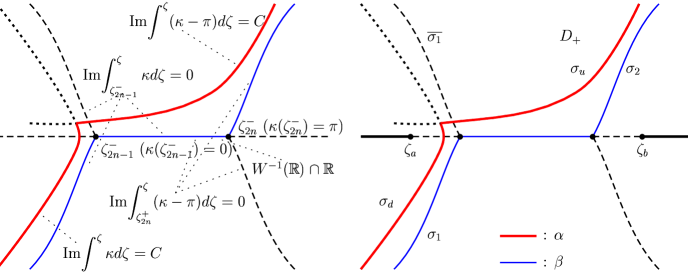
Denote by $\zeta_{a}$ and $\zeta_{b}$ the branch points situated on ${\mathbb{R}}$ and, respectively, closest to $\zeta_{2n-1}^{-}$ on its left and closest to $\zeta_{2n}^{-}$ on its right. Let $\mathcal{D}$ be a regular domain obtained by cutting $S_{Y}$ along the Stokes lines $\sigma_{1}$, and $\sigma_{2}$ and along the real intervals $(-\infty,\zeta_{a}]$ and $[\zeta_{b},\infty)$, see Fig. 8. We prove

Proposition 5.1.

If $\delta$ is sufficiently small, then, $f$ has standard behavior

(5.7) $$f=e^{\frac{i}{\varepsilon}\int_{\zeta_{0}}^{\zeta}\kappa d\zeta}\left(\Psi_{+}(x,\zeta,\zeta_{0})+o(1)\right)$$

in the whole domain $\mathcal{D}$.

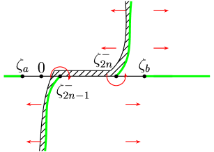
The rest of this section is devoted to the proof of Proposition 5.1. The proof is naturally divided into “elementary” steps. At each step, applying just one of the three continuation tools (i.e. the Rectangle Lemma, the Adjacent domain principle and the Stokes Lemma), we justify the standard behavior of $f$ on one more subdomain of $\mathcal{D}$. Fig. 8 shows where we use each of the continuation principles. Full straight arrows indicate the use of the Rectangle Lemma, circular arrows indicate the use of the Stokes Lemma, and, in the hatched domains, we use the Adjacent Canonical Domain Principle.

Again, the analysis of the cases $n$ odd and $n$ even are analogous. For sake of definiteness, we assume that $n$ odd and consider only this case. We shall use

Lemma 5.2.

If $n$ is odd, then, in $\mathcal{D}\setminus[\zeta_{2n-1}^{-},\zeta_{2n}^{-}]$,

• to the left of the Stokes lines $\sigma_{1}$ and $\sigma_{2}$, one has ${\rm Im}\,\kappa>0$;

• to the right of these Stokes lines, one has ${\rm Im}\,\kappa<0$.

Proof.  The sign of ${\rm Im}\,\kappa$ remains the same in any regular domain not intersecting $Z$. Moreover, the sign of ${\rm Im}\,\kappa$ changes to the opposite one as $\zeta$ intersects a connected component of $Z$ at a point where $W^{\prime}\neq 0$. So, in the connected subdomain of $\mathcal{D}\setminus[\zeta_{2n-1}^{-},\zeta_{2n}^{-}]$ to the left of $\sigma_{1}\cup[\zeta_{2n-1}^{-},\zeta_{2n}^{-}]\cup\sigma_{2}$, one has ${\rm Im}\,\kappa={\rm Im}\,(\kappa_{p}-\pi(n-1))={\rm Im}\,\kappa_{p}>0$ (here, we have used (5.6) for $n$ odd). To come from this subdomain to the connected subdomain of $\mathcal{D}\setminus[\zeta_{2n-1}^{-},\zeta_{2n}^{-}]$ to the right of $\sigma_{1}\cup[\zeta_{2n-1}^{-},\zeta_{2n}^{-}]\cup\sigma_{2}$, one has to intersect the interval $[\zeta_{2n-1}^{-},\zeta_{2n}^{-}]$ which is a connected component of $Z$. So, in the right subdomain, one has ${\rm Im}\,\kappa<0$. ∎

5.3.2. Behavior of $f$ between the lines $\gamma$ and $\beta$

To justify the standard asymptotics of $f$ in $\mathcal{D}$ between the lines $\gamma$ and $\beta$, we use the Adjacent Canonical Domain Principle. Therefore, we need to describe a canonical domain enclosing $\gamma$ (more precisely, the part situated between $\gamma$ and $\beta$). We do this by means of the Trapezium Lemma 4.4 (first statement).

Figure 8. How to “continue” the asymptotics of $f$

Let us describe the domain $U$ and the curves $\gamma_{0}$, $\sigma_{d}$ and $\sigma_{u}$ needed to apply the Trapezium Lemma 4.4.

The domain $U$. It is the domain bounded by $\beta$, $\gamma$ and the lines ${\rm Im}\,\zeta={\rm Const}$ containing the ends of $\gamma$.

In view of Lemma 5.2, choosing the ends of $\gamma$ closer to the lines ${\rm Im}\,\zeta=\pm Y$ if necessary, we can assume that ${\rm Im}\,\kappa>0$ in the domain $U$.

The line $\sigma_{u}$. As the line $\sigma_{u}$, we take the line which belongs to the family ${\rm Im}\,\int^{\zeta}\kappa d\zeta={\rm Const}$ and intersects $\beta$ at $\tilde{\zeta}_{u}$ satisfying ${\rm Im}\,\tilde{\zeta}_{u}=Y$. Recall that $\gamma$ is constructed in the $\delta$-neighborhood of $\beta$ where $\delta$ can be fixed arbitrarily small. One has

Lemma 5.3.

The line $\sigma_{u}$ enters $U$ at $\tilde{\zeta}_{u}$ and goes upwards. If $\delta$ is sufficiently small, then, $\sigma_{u}$ intersects $\gamma$ at an internal point of $\gamma$.

Proof.  The main tool of this proof is Lemma 4.2. Below, we use it without further notice. Recall that, above the real line, $\beta$ coincides with the Stokes line $\sigma_{2}$. So, it is tangent to the vector field $\overline{\kappa(\zeta)-\pi}$. The line $\sigma_{d}$ is tangent to the vector field $\overline{\kappa(\zeta)}$. In $U$, and in particular at $\tilde{\zeta}_{u}$, one has ${\rm Im}\,\kappa>0$. Therefore, at $\tilde{\zeta}_{u}$, the tangent vector to $\beta$ (oriented upwards) is directed to the right with respect to the tangent vector to $\sigma_{u}$ (oriented upwards). So, $\sigma_{u}$ enters $U$ at $\tilde{\zeta}_{u}$ going upwards. As ${\rm Im}\,\kappa\neq 0$ in $U$, it stays vertical in $U$. Note that $\sigma_{u}$ is independent of $\delta$. So, if $\delta$ is small enough, then $\sigma_{u}$ intersects $\gamma$. ∎

The line $\sigma_{d}$. It is the line of Stokes type ${\rm Im}\,\int^{\zeta}\kappa d\zeta={\rm Const}$ that intersects $\beta$ at $\tilde{\zeta}_{d}$ satisfying ${\rm Im}\,\tilde{\zeta}_{d}=-Y$. One has

Lemma 5.4.

The line $\sigma_{d}$ enters $U$ at $\tilde{\zeta}_{d}$ and goes downwards. If $\delta$ is sufficiently small, then $\sigma_{d}$ intersects $\gamma$ at an internal point.

The proof of this lemma being similar to the proof of Lemma 5.3, we omit it.

The line $\gamma_{0}$. We choose $\delta$ so that both $\sigma_{u}$ and $\sigma_{d}$ intersect $\gamma$. Then, $\gamma_{0}$ is the segment of $\gamma$ between its intersection points with $\sigma_{d}$ and $\sigma_{u}$.

5.3.3. Describing the curve $\tilde{\gamma}$

Let us describe the canonical line $\tilde{\gamma}$ needed to apply the first variant of the Trapezium Lemma. As for $\gamma$, using Lemma 5.1, we can construct $\tilde{\gamma}$ so that it be arbitrarily close to $\beta$ and strictly between $\gamma_{0}$ and $\beta$.

As $\sigma_{u}$ and $\sigma_{d}$ intersect $\gamma$ and $\beta$, they also intersect $\tilde{\gamma}$.

5.3.4. Completing the analysis

By the Trapezium Lemma, the domain bounded by $\gamma_{0}$, $\sigma_{u}$, $\sigma_{d}$ and $\tilde{\gamma}$ is a part of the canonical domain enclosing $\gamma_{0}$. So, by the Adjacent Canonical Domain Principle, $f$ has the standard behavior here.

As $\tilde{\gamma}$ can be constructed arbitrarily close to $\beta$, we conclude that $f$ has the standard behavior in the whole domain bounded by $\beta$, $\gamma$ and the lines $|{\rm Im}\,\zeta|=Y$.

5.4. Behavior of $f$ to the left of $\gamma$

We justify the standard behavior of $f$ in $\mathcal{D}$ to the left of $\gamma$ by means of the Rectangle Lemma.

Let us describe $R$, the rectangle used to apply Lemma 4.3: it is the part of $\mathcal{D}$ between the canonical line $\gamma_{1}=\gamma$ and a vertical line in $\mathcal{D}$, say $\gamma_{2}$, staying to the left of $\gamma$ and going from ${\rm Im}\,\zeta=-Y$ to ${\rm Im}\,\zeta=Y$.

By Lemma 5.2, in $R$, the imaginary part of $\kappa$ is positive. Moreover, $f$ has standard behavior in a neighborhood of $\gamma$. So, by the Rectangle Lemma, $f$ has standard behavior in $R$.

Pick $\zeta\in\mathcal{D}$ to the left of $\gamma$. As the vertical curve $\gamma_{2}\subset\mathcal{D}$ can be taken so that $\zeta\in R$, we see that $f$ has standard behavior in the whole part of $\mathcal{D}$ situated to the left of $\gamma$.

5.5. Behavior of $f$ to the right of $\sigma_{1}$

First, by means of the Stokes Lemma, Lemma 4.5, we show that $f$ has standard behavior to the right of $\sigma_{1}$ in its small neighborhood.

Let $\tilde{V}_{1}$ be a sufficiently small constant neighborhood of $\sigma_{1}$ and set $V_{1}=\tilde{V}_{1}\cap S_{Y}$. Show that $f$ has standard behavior in $V_{1}\setminus\sigma_{1}$. The Stokes lines $\sigma_{1}$, $\overline{\sigma_{1}}$ and $[\zeta_{2n-1}^{-},\zeta_{2n}^{-}]$ divide $V_{1}$ into three sectors. By the previous steps, we know that $f$ has the standard behavior in $V_{1}$ outside the sector $\mathcal{S}$ bounded by the Stokes lines $\sigma_{1}$ and $[\zeta_{2n-1}^{-},\zeta_{2n}^{-}]$. The Stokes line $\sigma_{1}$ is vertical. By Lemma 5.2, in $V_{1}$, to the left of $\sigma_{1}$, the imaginary part of the complex momentum is positive; thus, the Stokes Lemma implies that $f$ has standard behavior inside $V_{1}\setminus\sigma_{1}$. Recall that the leading term of the asymptotics of $f$ in $\mathcal{S}$ is obtained by analytic continuation from the rest of $V_{1}$ around the branch point $\zeta_{2n-1}^{-}$ avoiding $\sigma_{1}$.

Having justified the standard behavior of $f$ to the right $\sigma_{1}$ in a small neighborhood of $\sigma_{1}$, we justify it in in the rest of the subdomain of $\mathcal{D}\cap\{-Y<{\rm Im}\,\zeta<0\}$ situated to the right of $\sigma_{1}$ by means of the Rectangle Lemma. The argument is similar to that carried out in subsection 5.4. So, we omit the details.

5.6. Behavior of $f$ along the interval $(\zeta_{2n-1}^{-},\zeta_{2n}^{-})$

In the previous steps, we have justified the standard behavior of $f$ both above and below the real interval $(\zeta_{2n-1}^{-},\zeta_{2n}^{-})$. We show now that $f$ has standard behavior also in this interval.
By section 5.5, we know that $f$ has standard behavior in a neighborhood of $\zeta_{2n-1}^{-}$ cut along $\sigma_{1}$. Moreover, $f$ can not have the standard behavior in a neighborhood $\zeta_{2n}^{-}$ (as $\zeta_{2n}^{-}$ is a branch point). Hence, there exists $a\in(\zeta_{2n-1}^{-},\zeta_{2n}^{-}]$ such that $f$ has the standard behavior in a neighborhood of any point in $(\zeta_{2n-1}^{-},a)$. Assume that $a<\zeta_{2n}^{-}$. Let $\alpha$ be a segment of the line ${\rm Re}\,\zeta=a$ connecting a point $a_{1}\in{\mathbb{C}}_{-}$ to a point $a_{2}\in{\mathbb{C}}_{+}$. One has $0<\kappa(a)<\pi$. This implies that, if $\alpha$ is small enough, then, $\alpha$ is a canonical line. The solution $f$ has the standard behavior to the left of $\alpha$. By the Adjacent Canonical Domain Principle, $f$ has standard behavior in any local canonical domain enclosing $\alpha$, thus, in a constant neighborhood of $a$. So, we obtain a contradiction, and, thus, $a=\zeta_{2n}^{-}$. This completes the analysis of $f$ along $(\zeta_{2n-1}^{-},\zeta_{2n}^{-})$.

5.7. Behavior of $f$ to the right of $\sigma_{2}$

One studies $f$ to the right of $\sigma_{2}$ in the same way as we have studied it to the right of $\sigma_{1}$: first, using the Stokes Lemma, one justifies the standard behavior to the right of $\sigma_{2}$, in a small neighborhood of $\sigma_{2}$, and, then, applying the Rectangle Lemma, one proves that $f$ has the standard behavior in the rest of the subdomain of $\mathcal{D}$ to the right of this neighborhood. We omit further details.
The analysis of $f$ to the right of $\sigma_{2}$ completes the proof of the Proposition 5.1. ∎

5.8. Normalization of $f$

To fix the normalization of the leading term of the asymptotics of $f$, we choose the normalization point $\zeta_{0}$ in $\mathcal{D}$ and, in a neighborhood of $\zeta_{0}$, we choose a branch of the function $\sqrt{k^{\prime}(\mathcal{E}(\zeta))}$ in the definition of $\Psi_{+}$.
As the normalization point, we take $\zeta_{0}$ such that

(5.8) $$\zeta_{2n-1}^{-}<\zeta_{0}<\zeta_{2n}^{-}$$

Inside any spectral band of the periodic operator, $k^{\prime}(\mathcal{E})$ does not vanish, and there are no poles of the Bloch solution $\psi(x,\mathcal{E})$. So, $\mathcal{E}(\zeta_{0})\not\in P\cup Q$, and the solution $\Psi_{+}$ is well defined.
To fix the branch of $\sqrt{k^{\prime}}$, we note that, inside any spectral band of the periodic operator, the main branch of the Bloch quasi-momentum, $k_{p}$, is real and satisfies $k_{p}^{\prime}>0$. So, we fix $\sqrt{k^{\prime}}$ so that

(5.9) $$\sqrt{k^{\prime}(\mathcal{E}(\zeta))}>0,\quad\zeta_{2n-1}^{-}<\zeta<\zeta_{2n}^{-}.$$

6. The consistent basis

Up to now, we have constructed $f$, one consistent solution to (4.1) with known asymptotic behavior in the domain $\mathcal{D}$. We now construct another consistent solution $f^{*}$ so that $(f,f^{*})$ form a consistent basis.

6.1. Preliminaries

For $\zeta\in{\mathcal{D}}^{*}$, the symmetric to $\mathcal{D}$ with respect to the real line, we define

(6.1) $$f^{*}(x,\zeta,E)=\overline{f(x,\overline{\zeta},\overline{E})}.$$

As $W$ is real analytic, the function $f^{\ast}$ is also a solution of (4.1); it satisfies the consistency condition as $f$ does. In the next subsections, we first study its asymptotic behavior; then, we compute the Wronskian $w(f,f^{*})$. We show that, in $S_{Y}$, it has the form ${\rm Const}\,(1+o(1))$. Here, ${\rm Const}$ is a non-zero constant, and $o(1)$ is a function which can depend on $\zeta$. Finally, we modify the solution $f$ so that it still have the standard behavior in $\mathcal{D}$, and $w(f,f^{*})$ be constant.

6.2. The asymptotics of $f^{*}$

Note that $\mathcal{D}\cap\mathcal{D}^{*}$ contains the interval $\mathfrak{z}=(\zeta_{2n-1}^{-},\zeta_{2n}^{-})\subset{\mathbb{R}}$. One has

Lemma 6.1.

In $\mathcal{D}^{*}$, the solution $f^{*}$ has the standard behavior

(6.2) $$f\sim e^{-\frac{i}{\varepsilon}\int_{\zeta_{0}}^{\zeta}\kappa_{*}d\zeta}\,\Psi_{-,*}(x,\zeta,\zeta_{0}),$$

where

• $\kappa_{*}$ is the branch of the complex momentum which coincides with $\kappa$ on $\mathfrak{z}$ and is analytic in $\mathcal{D}^{*}$,

• $\Psi_{-,*}$ is the canonical Bloch solution which coincides with $\Psi_{-}$ (corresponding to $\Psi_{+}$ from the asymptotics of $f$) on $\mathfrak{z}$ and is analytic in $\mathcal{D}^{*}$.

Proof.  Recall that, by Proposition 5.1, $f$ has the standard behavior (5.7) in the domain $\mathcal{D}$.
The statement of Lemma 6.1 follows from Proposition 5.1, the definition of $f^{*}$ and the relation

(6.3) $$\overline{\exp\left(\frac{i}{\varepsilon}\int_{\zeta_{0}}^{\bar{\zeta}}\kappa d\zeta\right)\,\Psi_{+}(x,\bar{\zeta},\zeta_{0})}=\exp\left(-\frac{i}{\varepsilon}\int_{\zeta_{0}}^{\zeta}\kappa_{*}d\zeta\right)\,\Psi_{-,*}(x,\zeta,\zeta_{0}).\quad\quad\zeta\in\mathcal{D}^{*}.$$

Let us prove this relation. As both the right and left hand sides of (6.3) are analytic in $\zeta$, it suffices to check (6.3) along the interval $\mathfrak{z}$. Recall that the interval $[\zeta_{2n-1}^{-},\zeta_{2n}^{-}]$ is a connected component of $Z$. This implies that

(6.4) $$\overline{\kappa(\zeta)}=\kappa(\zeta),\quad\overline{\psi_{+}(x,\mathcal{E}(\zeta))}=\psi_{-}(x,\mathcal{E}(\zeta)),\quad\zeta\in\mathfrak{z},$$

where $\psi_{\pm}(x,\mathcal{E})$ are two different branches of the Bloch solution $\psi(x,\mathcal{E})$.
As $\zeta_{0}$ satisfies (5.8), relation (6.3) follows from the first relation in (6.4) and the relation

(6.5) $$\overline{\Psi_{+}(x,\zeta,\zeta_{0})}=\Psi_{-}(x,\zeta,\zeta_{0}),\quad\zeta\in\mathfrak{z}.$$

To check (6.5), we recall that $\Psi_{\pm}$ are defined in section 4.1.2 by formula (4.7). Therefore, relation (6.5) follows from (5.9), the second relation in (6.4) and the last property of $\omega$ listed in the section 3.3. This completes the proof of Lemma 6.1. ∎

6.3. The Wronskian of $f$ and $f^{*}$

The solutions $f$ and $f^{*}$ are analytic in the strip $S_{Y}$. Here, we study their Wronskian. As both $f$ and $f^{*}$ satisfy condition (4.2), the Wronskian is $\varepsilon$-periodic in $\zeta$. One has

Lemma 6.2.

The Wronskian of $f$ and $f^{*}$ admits the asymptotic representation:

(6.6) $$w(f,f^{*})=w(\Psi_{+},\Psi_{-})|_{\zeta=\zeta_{0}}+g,\quad\quad\zeta\in S_{Y}.$$

Here, $g$ is a function analytic in $S_{Y}$, such that, along the real line, ${\rm Re}\,g=0$. Moreover, $g=o(1)$ locally uniformly in any compact of $S_{Y}$ provided that $E$ is in a sufficiently small complex neighborhood of $E_{0}$.

Remark 6.1.

Note that

1. $w(\Psi_{+},\Psi_{-})|_{\zeta=\zeta_{0}}\neq 0$ (as $\mathcal{E}(\zeta_{0})\not\in P\cup Q$, see (5.8) and the comments to it);

2. $w(\Psi_{+},\Psi_{-})|_{\zeta=\zeta_{0}}\in i{\mathbb{R}}$ (due to (6.5)).

Proof.  The domain $\mathcal{D}\cap\mathcal{D}^{\ast}$ contains the “rectangle” $R$ bounded by the lines $\sigma_{1}\cup\overline{\sigma_{1}}$, $\sigma_{2}\cup\overline{\sigma_{2}}$ and ${\rm Im}\,\zeta=\pm Y$. So, in $R$, the solutions $f$ and $f^{*}$ have the standard behavior (5.7) and (6.2). Consider the functions $\kappa_{*}$ and $\Psi_{-,*}$ from (6.2). Their definitions, see Lemma 6.1, imply that

$$\kappa_{*}=\kappa,\quad\Psi_{-,*}=\Psi_{-},\quad\quad\zeta\in R.$$

Using this information and (5.7) and (6.2), one obtains

(6.7) $$w(f,f^{*})=w(\Psi_{+}(\cdot,\zeta),\Psi_{-}(\cdot,\zeta))+g,\quad g=o(1),\quad\quad\zeta\in R.$$

Being obtained using standard behavior, this estimate is uniform in $\zeta$ in any compact of $R$ provided $E$ be in a sufficiently small neighborhood of $E_{0}$. By (4.8), the first term in the left hand side of (6.7) coincides with the first term in (6.6). So, we only have to check that $g$ has all the properties announced in Lemma 6.2. As $w(f,f^{*})$ is $\varepsilon$-periodic, so is $g$. Furthermore, $ig$ is real analytic as $iw(f,f^{*})$ and $iw(\Psi_{+},\Psi_{-})|_{\zeta=\zeta_{0}}$ are. This completes the proof of Lemma 6.2. ∎

6.4. Modifying $f$

As $g$, the error term in (6.6) may depend on $\zeta$, we redefine the solution $f$:

$$f:=f/\nu,\quad\nu=\sqrt{1+g/w(\Psi_{+},\Psi_{-})|_{\zeta=\zeta_{0}}}.$$

In terms of this new solution $f$, we define the new $f^{*}$ by (6.1). These are the basis solutions the monodromy matrix of which we shall study. For these “new” functions $f$ and $f^{*}$, we have

Theorem 6.1.

The solutions $f$ and $f^{*}$ satisfy the condition (4.2) and

(6.8) $$w(f,f^{\ast})=w(\Psi_{+},\Psi_{-})|_{\zeta=\zeta_{0}}.$$

Moreover, $f$ has the standard behavior (5.7) in $\mathcal{D}$, and $f^{*}$ has the standard behavior (6.2) in $\mathcal{D}^{*}$.

Proof.  Let $\zeta$ be in a fixed strip $\{y_{1}<{\rm Im}\,\zeta<y_{2}\}\subset S_{Y}$, and let $\varepsilon$ be sufficiently small. We use Lemma 6.2 and Remark 6.1. Recall that $g$ is $\varepsilon$-periodic in $\zeta$. So, $\nu$ is $\varepsilon$-periodic, and $f$ and $f^{*}$ remain consistent. Furthermore, note that $\nu$ is real analytic. This implies (6.8). Finally, as $\nu=1+o(1)$, the new solutions $f$ and $f^{*}$ still have the “old” standard asymptotic behavior in $\mathcal{D}$ and $\mathcal{D}^{*}$ respectively.∎

7. General properties of the monodromy matrix for the basis $\{f,f^{*}\}$

In the previous section (see Theorem 6.1), we have constructed $(f,f^{*})$, a consistent basis of solutions of (4.1). If we return to the variables of the initial equation (0.1), we get a consistent basis of (0.1). The matrix discussed in Theorem 1.4 is the monodromy matrix obtained for this basis. In this short section, we check some of its properties.

Instead of coming back to the initial variables, we continue to work in the variables (5.1). The definition of the monodromy matrix (1.6) takes the form

(7.1) $$F(x,\zeta+2\pi)=M(\zeta)F(x,\zeta),\quad F=\begin{pmatrix}f(x,\zeta)\\ f^{*}(x,\zeta)\end{pmatrix},$$

and the matrix $M$ becomes $\varepsilon$-periodic in $\zeta$.
As the basis solutions $f$ and $f^{\ast}$ are related by (6.1), the monodromy matrix has the form (1.10).
The definition of the monodromy matrix (7.1) implies that

(7.2) $$a(\zeta)\equiv M_{11}(\zeta)=\frac{w(f(x+2\pi,\zeta),f^{*}(x,\zeta))}{w(f(x,\zeta),f^{*}(x,\zeta))},\quad b(\zeta)\equiv M_{12}(\zeta)=\frac{w(f(x,\zeta),f(x,\zeta+2\pi))}{w(f(x,\zeta),f^{*}(x,\zeta))}.$$

Finally, we note that the monodromy matrix is analytic in $\zeta$ in the strip $S_{Y}$ and in $E$ in a constant neighborhood of $E_{0}$. Indeed, as the solutions $f$ and $f^{*}$ are analytic functions of both variables, so are the Wronskians in (7.2). Moreover, by (6.8), the Wronskian in the denominators in (7.2) does not vanish. Hence, we have proved the

Lemma 7.1.

The monodromy matrix corresponding to the basis $\{f,f^{*}\}$ satisfies (7.1), is analytic and $\varepsilon$-periodic in $\zeta\in S_{Y}$, analytic in $E$ in a constant neighborhood of $E_{0}$ and has the form (1.10). Its coefficients are given by (7.2).

8. General asymptotic formulas

To compute the asymptotics of the monodromy matrix defined above, we only need to compute the Wronskians in the numerators in (7.2). These Wronskians depend on $\zeta$ and have different asymptotics in the lower and upper half planes. Rather than repeating similar computations many times, in the present section, we obtain a general asymptotic formula for the Wronskian of two solutions having standard behavior.

8.1. General setting

In this subsection, we do not suppose that $W$ be periodic. Fix $E=E_{0}$. Assume that $h$ and $g$ are two solutions of (4.1) having the standard asymptotic behavior in regular domains $D_{h}$ and $D_{g}$:

(8.1) $$h\sim e^{\frac{i}{\varepsilon}\int_{\zeta_{h}}^{\zeta}\kappa_{h}d\zeta}\,\Psi_{h}(x,\zeta),\quad g\sim e^{\frac{i}{\varepsilon}\int_{\zeta_{g}}^{\zeta}\kappa_{g}d\zeta}\,\Psi_{g}(x,\zeta).$$

Here, $\kappa_{h}$ and $\kappa_{g}$ are branches of the complex momentum analytic in $D_{h}$ and $D_{g}$,  $\Psi_{h}$ and $\Psi_{g}$ are canonical Bloch solutions $\Psi_{+}$ defined on $D_{h}$ and $D_{g}$, and $\zeta_{h}$ and $\zeta_{g}$ are the normalization points for $h$ and $g$.
As the solutions $h$ and $g$ satisfy the consistency condition, their Wronskian is $\varepsilon$-periodic in $\zeta$. We now describe the asymptotics of this Wronskian and of its Fourier coefficients. We first introduce several simple useful objects.
Below, we assume that $D_{g}\cap D_{h}$ contains a simply connected domain, say $d$.

8.1.1. Arcs

Let $\gamma$ be a regular curve going from $\zeta_{g}$ to $\zeta_{h}$ in the following way: staying in $D_{g}$, it goes from $\zeta_{g}$ to some point in $d$, then, staying in $D_{h}$, it goes to $\zeta_{h}$. We say that $\gamma$ is an arc associated to the triple $h$, $g$ and $d$.
As $d$ is simply connected, all the arcs associated to one and the same triple can naturally be considered as equivalent; we denote them by $\gamma(h,g,d)$.

Let us continue $\kappa_{h}$ and $\kappa_{g}$ analytically along $\gamma(h,g,d)$. The analysis performed in section 4.1.1, see (4.5), yields, that, for $V$ a small neighborhood of $\gamma$, one has

(8.2) $$\kappa_{g}(\zeta)=\sigma\kappa_{h}(\zeta)+2\pi m,\quad\quad m\in{\mathbb{Z}},\quad\sigma\in\{-1,+1\},\quad\zeta\in V.$$

We call $\sigma=\sigma(h,g,d)$ the signature of $\gamma$, and $m=m(h,g,d)$ the index of $\gamma(h,g,d)$.

8.1.2. Meeting domains

Let $d$ be as above. We call $d$ a meeting domain, if, in $d$, the functions ${\rm Im}\,\kappa_{h}$ and ${\rm Im}\,\kappa_{g}$ do not vanish and are of opposite sign.
Note that, for small values of $\varepsilon$, the increasing and decreasing of $h$ and $g$ is determined by the exponential factors $e^{\frac{i}{\varepsilon}\,\int^{\zeta}\kappa d\zeta}$. So, roughly, in a meeting domain, along the lines ${\rm Im}\,\zeta={\rm Const}$, the solutions $h$ and $g$ increase in opposite directions.

8.1.3. The amplitude and the action of an arc

We call the integral

$$S(h,g,d)=\int_{\gamma(h,g,d)}\kappa_{g}d\zeta$$

the action of the arc $\gamma(h,g,d)$. Clearly, the action takes the same value for equivalent arcs.

Assume that $\mathcal{E}(\zeta)\not\in P\cup Q$ along $\gamma=\gamma(h,g,d)$. Consider the function $q_{g}=\sqrt{k^{\prime}(\mathcal{E}(\zeta))}$ and the $1$-form $\Omega_{g}(\mathcal{E}(\zeta))$ in the definition of $\Psi_{g}$. Continue them analytically along $\gamma$. Put

(8.3) $$A(h,g,\gamma)=\left.\left(q_{g}/q_{h}\right)\right|_{\zeta=\zeta_{h}}\,e^{\int_{\zeta_{g}}^{\zeta_{h}}\Omega_{g}},$$

We call $A$ the amplitude of the arc $\gamma$. The first three properties of $\Omega$ listed in section 3.3 imply

Lemma 8.1.

The amplitudes of two equivalent arcs $\gamma(h,g,d)$ coincide.

8.1.4. Fourier coefficients

Let $S(d)$ be the smallest strip of the form $\{C_{1}<{\rm Im}\,\zeta<C_{2}\}$ containing the domain $d$. One has

Proposition 8.1.

Let $d=d(h,g)$ be a meeting domain for $h$ and $g$, and $m=m(h,g,d)$ be the corresponding index. Then,

(8.4) $$w(h,g)=w_{m}\,e^{\frac{2\pi im}{\varepsilon}(\zeta-\zeta_{h})}(1+o(1)),\quad\zeta\in S(d),$$

and $w_{m}$ is the constant given by

(8.5) $$w_{m}=A(h,g,d)\,e^{\frac{i}{\varepsilon}\,S(h,g,d)}\,w(\Psi_{+}(\cdot,\zeta_{h}),\Psi_{-}(\cdot,\zeta_{h})),$$

where $\Psi_{+}=\Psi_{h}$ and $\Psi_{-}$ is “complementary” to $\Psi_{+}$. The asymptotics (8.4) is uniform in $\zeta$ and $E$ when $\zeta$ stays in a fixed compact of $S(d)$ and $E$ in a small enough constant neighborhood of $E_{0}$.

Note that the factor $w_{m}$ is the leading term of the asymptotics of the $m$-th Fourier coefficient of $w(h,g)$.

Proof.  For $\zeta\in D_{g}$, let $\gamma_{g}(\zeta)$ be a curve in $D_{g}$ from $\zeta_{g}$ to $\zeta$. Similarly, define $\gamma_{h}(\zeta)$.
First, we check that, for $\zeta\in d$, one has

(8.6) $$e^{\frac{i}{\varepsilon}\,\int_{\gamma_{g}(\zeta)}\kappa_{g}\,d\zeta}=e^{\frac{i}{\varepsilon}\,S(h,g,d)}\,e^{\frac{2\pi im}{\varepsilon}\,(\zeta-\zeta_{h})}\,\,\left(e^{-\frac{i}{\varepsilon}\,\int_{\gamma_{h}(\zeta)}\kappa_{h}\,d\zeta}\right),$$

(8.7) $$\Psi_{g}(x,\zeta)=A(h,g,d)\,\Psi_{-}(x,\zeta),$$

where $\Psi_{-}$ is the canonical Bloch solution “complementary” to $\Psi_{+}=\Psi_{h}$ in a neighborhood of $\gamma_{h}(\zeta)$.
As $d$ is a meeting domain, in a neighborhood of $\gamma(h,g,d)$, one has

(8.8) $$\kappa_{g}=-\kappa_{h}+2\pi\,m$$

This implies relation (8.6).
Check (8.7). Let $\gamma=\gamma(h,g,d)$ be an arc such that $\mathcal{E}(\gamma)\cap(P\cup Q)=\emptyset$. Continue $q_{g}$, $\Omega_{g}$ and $\psi_{g}$ analytically along the arc $\gamma(h,g,d)$. Note that $q_{g}$ and $q_{h}$ are two different branches of the function $\sqrt{k^{\prime}(E-W(\zeta))}$. So, they differ at most by a constant factor. Therefore, in a neighborhood of $\zeta_{h}$, we get

(8.9) $$\Psi_{g}(x,\zeta)=A(h,g,d)\,q_{h}(\mathcal{E}(\zeta))e^{\int_{\gamma_{h}(\zeta)}\Omega_{g}}\psi_{g}(x,\mathcal{E}(\zeta)).$$

Now, recall that, in a neighborhood of $\zeta_{h}$, there are only two branches of $\Omega$ and $\psi$. Denote them by $\psi_{\pm}$ and $\Omega_{\pm}$ so that $\psi_{+}=\psi_{h}$ and $\Omega_{+}=\Omega_{h}$. Then, either $\psi_{g}=\psi_{-}$ and $\Omega_{g}=\Omega_{-}$ or $\psi_{g}=\psi_{+}$ and $\Omega_{g}=\Omega_{+}$. To choose between these two variants, we recall that the Bloch quasi-momentum of a Bloch solution is defined modulo $2\pi$. Note that $\kappa_{h}$ is the Bloch quasi-momentum of $\psi_{+}$, and $\kappa_{g}$ is the Bloch quasi-momentum of $\psi_{g}$. By (8.8), we get $\kappa_{g}=-\kappa_{h}\,{\rm mod}\,2\pi$. So, $\kappa_{g}$ must be the Bloch quasi-momentum of $\psi_{-}$. Thus, we have $\psi_{g}=\psi_{-}$ and $\Omega_{g}=\Omega_{-}$, and (8.9) implies relation (8.7) in a neighborhood of $\zeta_{h}$. By analyticity, it stays valid in $d$.
As $d\subset D_{h}\cap D_{g}$, both $h$ and $g$ have standard behavior in $d$. Substituting the asymptotics of $f$ and $g$ into $w(f,g)$, and using (8.6) and (8.7), one easily obtains

(8.10) $$w(h,g)=A(h,g,d)\,e^{\frac{i}{\varepsilon}\,S(h,g,d)}\,e^{\frac{2\pi im}{\varepsilon}\,(\zeta-\zeta_{h})}\,(w(\Psi_{+}(\cdot,\zeta),\Psi_{-}(\cdot,\zeta))+o(1)),\quad\zeta\in d.$$

As $w(\Psi_{+}(\cdot,\zeta),\Psi_{-}(\cdot,\zeta))$ is independent of $\zeta$ and $\varepsilon$ and is non-zero (see (4.8) and comments to it), we get (8.4). As this asymptotic was obtained using the standard behavior of $h$ and $g$, it has all the announced uniformity properties. This completes the proof of Proposition 8.1. ∎

8.2. The index $m$ and the periods when $W$ is periodic

Here, we only assume that $W$ is $2\pi$-periodic and real analytic in $\zeta$ (i.e. we do not assume anything on the critical points of $W$), and that $E$ is fixed. We describe the computation of the index $m$ in the special case that one encounters when computing monodromy matrices.

8.2.1. Periods

Pick $\zeta_{0}$, a regular point. Consider a regular curve $\gamma$ going from $\zeta_{0}$ to $\zeta_{0}+2\pi$. Fix $\kappa$, a branch of the complex momentum that is continuous on $\gamma$. We call the couple $(\gamma,\kappa)$ a period.
Let $(\gamma_{1},\kappa_{1})$ and $(\gamma_{2},\kappa_{2})$ be two periods. Assume that one can continuously deform $\gamma_{1}$ into $\gamma_{2}$ without intersecting any branching point. This defines an analytic continuation of $\kappa_{1}$ to $\gamma_{2}$. If the analytic continuation coincides with $\kappa_{2}$, we say that the periods are equivalent.
Consider the branch $\kappa$ along the curve $\gamma$ of a period $(\gamma,\kappa)$. In a neighborhood of $\zeta_{0}$, the starting point $\gamma$, one has

(8.11) $$\kappa(\zeta+2\pi)=\sigma\kappa(\zeta)+2\pi m,\quad\sigma\in\{\pm 1\},\quad m\in{\mathbb{Z}}.$$

The numbers $\sigma=\sigma(\gamma,\kappa)$ and $m=m(\gamma,\kappa)$ are called the signature and the index of the period $(\gamma,\kappa)$. The numbers $m$ (resp. $\sigma$) coincide for equivalent periods.
Recall that $G$ is the pre-image with respect to $\mathcal{E}$ of the spectral gaps of $H_{0}$. One has

Lemma 8.2.

Let $(\gamma,\kappa)$ be a period such that $\gamma$ begins at a point $\zeta_{0}\not\in G$. Assume that $\gamma$ intersects $G$ exactly $N$ times ($N\in{\mathbb{N}}^{*}$) and that, at all intersection points, $W^{\prime}\neq 0$. Let $r_{1}$, $r_{2}$, …, $r_{N}$ be the values that ${\rm Re}\,\kappa$ takes consecutively at these intersection points as $\zeta$ moves along $\gamma$ from $\zeta_{0}$ to $\zeta_{0}+2\pi$. Then,

(8.12) $$\sigma(\gamma,\kappa)=(-1)^{N},\quad m(\gamma,\kappa)=\frac{1}{\pi}\,(r_{N}-r_{N-1}+r_{N-2}-\dots+(-1)^{N-1}r_{1}).$$

Proof.  The image ${\mathcal{E}}(\gamma)$ of $\gamma$ by $\mathcal{E}:\,\zeta\mapsto E-W(\zeta)$ is a closed curve that starts and ends at ${\mathcal{E}}_{0}={\mathcal{E}}(\zeta_{0})$. We consider the curve $\mathcal{E}(\gamma)$ as open at $\mathcal{E}_{0}$. Along $\gamma$, we can write $\kappa(\zeta)=k(E-W(\zeta))$ where $k$ is a fixed analytic branch of the quasi-momentum. So, $\kappa(\zeta_{0})$ and $\kappa(\zeta_{0}+2\pi)$, the values of the complex momentum at the ends of $\gamma_{0}$, are related by the same formula as $k_{b}$ and $k_{e}$, the values of $k$ at the beginning and the end of curve ${\mathcal{E}}(\gamma_{0})$.
Since $W^{\prime}\neq 0$ at the points of intersection of $\gamma_{0}$ and $G$, ${\mathcal{E}}(\gamma_{0})$ intersects exactly $N$ times spectral gaps of the periodic operator.
As the values for both $m$ and $\sigma$ coincide for equivalent periods, it suffices to construct $\zeta_{0}$ so that ${\rm Im}\,\mathcal{E}_{0}\neq 0$.
Assume that a continuous curve begins at ${\mathcal{E}}_{0}$, goes along a strait line to one of the ends of a gap, then goes around this gap end along an infinitesimally small circle, and returns back to ${\mathcal{E}}_{0}$ along the same strait line. We call such a curve a simple loop. We distinguish the end and the beginning of the loop considering it as open at its endpoints. As ${\rm Im}\,{\mathcal{E}}_{0}\neq 0$, any simple loop intersects only one gap, namely, the gap around the end of which it goes.
Recall that the ends of the gaps coincide with the branching points of the Bloch quasi-momentum, and that these branching points are of square root type. So, in a neighborhood of a branching point, the corresponding branches of the Bloch quasi-momentum satisfy the relation

(8.13) $$k_{1}(E)+k_{2}(E)=2r,$$

where $r$ is the common value of these branches at the branching point. Note that $r$ is equal to the value of the real part of any of these branches on the spectral gap beginning at the branching point.
On a simple loop, fix a continuous branch of the quasi-momentum. Clearly, formula (8.13) also relates the values of the quasi-momentum at the ends of the loop when $r$ is the value of the quasi-momentum at the branching point inside the loop.
Recall that $k$ can be analytically continued onto the whole complex plane cut along the spectral gaps of $H_{0}$. Therefore, the value of $k$ at the end of ${\mathcal{E}}(\gamma_{0})$ is equal to the value of $k$ at the end of the curve consisting of $N$ simple loops and going successively around the branch points of $k$ with $k=r_{1},r_{2},\dots r_{N}$. So, taking (8.13) into account, we get

$$k_{e}=(-1)^{N}k_{b}+2(r_{N}-r_{N-1}+r_{N_{2}}-\dots r_{1}).$$

This implies (8.12) and completes the proof of Lemma 8.2.∎

8.2.2. Indices of periods

Let us come back to the computation of the index $m(h,g,d)$. One has

Lemma 8.3.

Let $\gamma=\gamma(h,g,d)$ be an arc such that $\zeta_{h}=\zeta_{g}+2\pi$. If, in a neighborhood of $\zeta_{g}$,

(8.14) $$\kappa_{g}(\zeta)=s\cdot\kappa_{h}(\zeta+2\pi),$$

where $s$ is either “+” or “-”, then,

(8.15) $$\sigma(h,g,d)=s\cdot\sigma(\gamma,\kappa_{g}),\quad m(h,g,d)=m(\gamma,\kappa_{g}).$$

Proof.  The pair $(\gamma(h,g,d),\kappa_{g})$ is a period. So, in a neighborhood of $\zeta_{g}$, one has $\kappa_{g}(\zeta+2\pi)=\sigma(\gamma,\kappa_{g})\kappa_{g}(\zeta)+2\pi m(\gamma,\kappa_{g})$. This and (8.14) imply that $\kappa_{g}(\zeta)=s\,\sigma(\gamma,\kappa_{g})\kappa_{h}(\zeta)+2\pi m(\gamma,\kappa_{g})$ in a neighborhood of $\zeta_{h}$. This implies the relations (8.15). ∎

9. Asymptotics of the monodromy matrix

We now compute the asymptotics of the coefficients $a$ and $b$ of the monodromy matrix for the basis $\{f,f^{*}\}$; in particular, we prove formulae (1.11) and (1.12). We concentrate on the case $n$ odd. The computations for $n$ even being similar, we omit them.
Recall that $a$ and $b$ are expressed via the Wronskians by formulae (7.2). We compute these Wronskians (and, thus, $a$ and $b$) using the construction from section 8.

9.1. The asymptotics of the coefficient $b$

By (7.2), we have to compute $w(f(\cdot,\zeta),f(\cdot,\zeta+2\pi))$. One applies the constructions of section 8. Now, one has

(9.1) $$h(x,\zeta)=f(x,\zeta),\quad g(x,\zeta)=(Tf)(x,\zeta)\quad\text{where}\quad(Tf)(x,\zeta)=f(x,\zeta+2\pi);$$

(9.2) $$D_{h}=\mathcal{D},\quad D_{g}=\mathcal{D}-2\pi;$$

(9.3) $$\zeta_{h}=\zeta_{0},\quad\zeta_{g}=\zeta_{0}-2\pi;$$

(9.4) $$\kappa_{h}(\zeta)=\kappa(\zeta),\quad\kappa_{g}(\zeta)=\kappa(\zeta+2\pi).$$

9.1.1. The asymptotics in the strip $0<{\rm Im}\,\zeta<Y$

Let us describe $d_{0}$, the meeting domain, and $\gamma_{0}=\gamma(f,Tf,d_{0})$, the arcs used to compute $w(f,Tf)$ in the strip $\{0<{\rm Im}\,\zeta<Y\}$.
The meeting domain. $d_{0}$ is the subdomain of the strip $0<{\rm Im}\,\zeta<Y$ between the Stokes lines $\sigma_{2}-2\pi$ and $\sigma_{2}$. Indeed, it follows from Lemma 5.2 and (9.4) that, in $d_{0}$, one has ${\rm Im}\,\kappa_{g}=-{\rm Im}\,\kappa_{h}<0$.
The arc. $\gamma_{0}$ connects the point $\zeta_{g}$ to $\zeta_{h}$. In view of (9.3), it defines the period $(\gamma_{0},\kappa_{g})$.
The index $m(f,Tf,d_{0})$. In view of (9.4), the arc $\gamma_{0}$ satisfies the assumption of Lemma 8.3. So, $m(f,Tf,d_{0})=m(\gamma_{0},\kappa_{g})$. Due to (9.4), $m(f,Tf,d_{0})=m(\gamma_{0}+2\pi,\kappa)$. To compute this integer, we use Lemma 8.2. Therefore, we have to compute $\kappa$ at the intersections of $\gamma_{0}+2\pi$ and $G$, the pre-image of the spectral gaps of $H_{0}$. The set $G\cap S_{Y}$ is described in section 5.1.3 where we have listed all its connected components.
Recall that $m$ takes the same value for all the periods equivalent to $(\gamma_{0}+2\pi,\kappa)$. We can deform $\gamma_{0}+2\pi$ into a curve, say $\gamma\subset\mathcal{D}$, so that

• $\gamma$ be to the left of the complex branch of $W^{-1}({\mathbb{R}})$ starting at $2\pi$ and staying in the upper half-plane,

• $(\gamma,\kappa)$ be a period equivalent to $(\gamma_{0}+2\pi,\kappa)$,

• $\gamma$ have the following intersections with the connected components of $G$ (for $m=0$, this curve is shown in Fig. 9): it once intersects the complex branch of $W^{-1}({\mathbb{R}})$ going upwards from $0$, once the interval $(\zeta_{2n}^{-},\zeta_{b})$ (the point $\zeta_{b}$ is defined in section 5.3.1), and, once the complex branch of $W^{-1}({\mathbb{R}})$ going upwards from $\zeta^{*}$.

Figure 9. Curves equivalent to $\gamma_{0}+2\pi$ and $\gamma_{1}+2\pi$ (when $m=0$)

Recall that ${\rm Re}\,\kappa(\zeta)$ is constant on any connected component of $G$. Therefore,

$$\begin{split}m(\gamma_{0}+2\pi,\kappa)=m(\gamma,\kappa)&=\frac{1}{\pi}\left(\left.{\rm Re}\,\kappa(\zeta)\right|_{\zeta_{2n-1}^{-}}-\left.{\rm Re}\,\kappa(\zeta)\right|_{\zeta_{2n}^{-}}+\left.{\rm Re}\,\kappa(\zeta)\right|_{\zeta\in\mathfrak{g}_{n+m}+i0}\right)\\ &=\frac{1}{\pi}\left(0-\pi+\left.{\rm Re}\,\kappa(\zeta)\right|_{\zeta\in\mathfrak{g}_{n+m}+i0}\right).\end{split}$$

To compute the last term in this formula, we recall that, in $D_{p,\rm left}$, the part of the domain $D_{p}$ (see section 5.1.4) situated to the left of the Stokes line $\sigma_{2}$, one has $\kappa=\kappa_{p}-\pi(n-1)$. In the domain $D_{p,{\rm right}}$, the part of $D_{p}$ situated to the right of $\sigma_{2}$, $\kappa$ is obtained by analytic continuation from $D_{p,{\rm left}}$ around the branch point $\zeta_{2n}^{-}$ passing below this branch point. As $\kappa_{p}(\zeta_{2n}^{-})=\pi n$, for $\zeta\in D_{p,{\rm right}}$, one has $\kappa(\zeta)=(2\pi n-\kappa_{p}(\zeta))-\pi(n-1)=\pi(n+1)-\kappa_{p}(\zeta)$. Along $\mathfrak{g}_{n+m}$, one has ${\rm Re}\,\kappa_{p}=\pi(n+m)$; hence, we get

(9.5) $$m(\gamma_{0}+2\pi,\kappa)=\frac{1}{\pi}(0-\pi+[\pi(n+1)-\pi(n+m)])=-m.$$

The result. Now, Proposition 8.1, formula (7.2) for $b$ and formula (6.8) imply formula (1.11) for $b$ with

(9.6) $$b_{-m}=A(f,Tf,d_{0})\,e^{\frac{i}{\varepsilon}S(f,Tf,d_{0})+\frac{2\pi im\zeta_{0}}{\varepsilon}},\quad(Tf)(x,\zeta)=f(x,\zeta+2\pi).$$

9.1.2. Asymptotics of $b$ below the real line

Describe $d_{1}$, the meeting domain, and compute the index $m(f,Tf,d_{1})$ needed to get the asymptotics of $w(f,Tf)$ in the strip $\{-Y<{\rm Im}\,\zeta<0\}$.
The meeting domain. $d_{1}$ is the subdomain of the strip $-Y<{\rm Im}\,\zeta<0$ situated between the Stokes lines $\sigma_{1}-2\pi$ and $\sigma_{1}$.
The index. The arc $\gamma_{1}=\gamma(f,Tf,d_{1})$ again defines a period, and $m(f,Tf,d_{1})=m(\gamma_{1}+2\pi,\kappa)$. The curve defining a period equivalent to $(\gamma_{1}+2\pi,\kappa)$ is shown in Fig. 9. As in the sequel of this computation we only use this curve, we call it $\gamma_{1}+2\pi$. To compute the index of this period, we compute ${\rm Re}\,\kappa$ at the intersections $\gamma_{1}+2\pi$ and $G$.
We can assume that $\gamma_{1}+2\pi$ satisfies:

• it is situated to the left of the complex branch of $W^{-1}({\mathbb{R}})$ in ${\mathbb{C}}_{-}$ starting at $2\pi$,

• it has the following intersections with $G$: it once intersects the complex branch of $W^{-1}({\mathbb{R}})$ going downward from $0$, once the interval $\mathfrak{g}_{n-1}$ and once the complex branch of $W^{-1}({\mathbb{R}})$ going downward from $\zeta^{*}$.

We get

$$m(\gamma_{1}+2\pi,\kappa)=\frac{1}{\pi}\left.{\rm Re}\,\kappa(\zeta)\right|_{\zeta\in\mathfrak{g}_{n+m}-i0}.$$

We have used the fact that the interval $\mathfrak{g}_{n-1}$ and the complex branch of $W^{-1}({\mathbb{R}})$ going downward from $0$ belong to the same connected component of $W^{-1}({\mathbb{R}})$. To finish the computation, we introduce the domain $D_{p}^{*}$, the symmetric of $D_{p}$ with respect to the real line. In $D_{p,\rm right}^{*}$, the part of this domain situated to the right of $\sigma_{1}$, $\kappa$ can be viewed as the analytic continuation of $\kappa_{p}-\pi(n-1)$ from $D_{p}$ across the interval $\mathfrak{z}_{n}^{-}$. Along the interval $\mathfrak{z}_{n}^{-}$, $\kappa_{p}$ is real. So, for $\zeta\in D_{p,\rm right}^{*}$, $\kappa(\zeta)=\overline{\kappa_{p}(\overline{\zeta})}-\pi(n-1)$, and

(9.7) $$m(\gamma_{1}+2\pi,\kappa)=\frac{1}{\pi}\left(\left.{\rm Re}\,\kappa_{p}(\zeta)\right|_{\zeta\in\mathfrak{g}_{n+m}+i0}-\pi(n-1)\right)=\frac{1}{\pi}(\pi(n+m)-\pi(n-1))=m+1$$

The result. Now, Proposition 8.1, formula (7.2) for $b$ and (6.8) imply formula (1.12) for $b$ with

(9.8) $$b_{m+1}=A(f,Tf,d_{1})\,e^{\frac{i}{\varepsilon}S(f,Tf,d_{1})-\frac{2\pi i(m+1)\zeta_{0}}{\varepsilon}},\quad(Tf)(x,\zeta)=f(x,\zeta+2\pi).$$

Figure 10. Curves $\tilde{\gamma}_{0}+2\pi$ and $\tilde{\gamma}_{1}+2\pi$ (when $m=0$)

9.2. The asymptotics of the coefficient $a$

The computations of the coefficient $a$ following the same scheme as those of $b$, we only outline them. Now,

(9.9) $$h=f^{*},\quad g=Tf;\quad\quad D_{h}=\mathcal{D}^{*},\quad D_{g}=\mathcal{D}-2\pi;$$

(9.10) $$\zeta_{h}=\zeta_{0},\quad\zeta_{g}=\zeta_{0}-2\pi;$$

(9.11) $$\kappa_{h}(\zeta)=-\overline{\kappa}(\bar{\zeta}),\quad\zeta\in D_{h},\quad\quad\kappa_{g}(\zeta)=\kappa(\zeta+2\pi),\quad\zeta\in D_{g}.$$

Recall that the complex momentum is real on $\mathfrak{z}_{n}^{-}$, and that $\zeta_{0}\in\mathfrak{z}_{n}^{-}$. This and relations (9.11) imply that

(9.12) $$\kappa_{g}(\zeta)=-\kappa_{h}(\zeta+2\pi),\quad\zeta\sim\zeta_{g}.$$

9.2.1. The asymptotics of $a$ above the real line

In this case, $\tilde{d}_{0}$, the meeting domain, is the subdomain of the strip $\{0<{\rm Im}\,\zeta<Y\}$ situated between the lines $\sigma_{2}-2\pi$ and $\overline{\sigma_{1}}$ (which is symmetric to $\sigma_{1}$ with respect to ${\mathbb{R}}$). The arc $\gamma(f^{*},Tf,\tilde{d}_{0})$ defines a period $(\tilde{\gamma}_{0},\kappa_{g})$; the curve $\tilde{\gamma}_{0}+2\pi$ is shown in Fig. 10. In view of (9.12), one is again in the case of Lemma 8.14, and, by means of Lemma 8.2, one obtains $m(f^{*},Tf,\tilde{d}_{0})=m(\tilde{\gamma}_{0}+2\pi,\kappa)=-m$. This yields formula (1.11) for $a$ with

(9.13) $$a_{-m}=A(f^{*},Tf,\tilde{d}_{0})\,e^{\frac{i}{\varepsilon}\,S(f^{*},Tf,\tilde{d}_{0})+\frac{2\pi im\zeta_{0}}{\varepsilon}}.$$

9.2.2. The asymptotics of $a$ below the real line

In this case, $\tilde{d}_{1}$, the meeting domain, is the subdomain of the strip $\{-Y<{\rm Im}\,\zeta<0\}$ situated between the lines $\overline{\sigma_{2}}$ (symmetric to $\sigma_{2}$ with respect to ${\mathbb{R}}$) and $\sigma_{1}-2\pi$. The arc $\gamma(h,g,\tilde{d}_{1})$ defines a period $(\tilde{\gamma}_{1},\kappa_{g})$; the curve $\tilde{\gamma}_{1}+2\pi$ is shown in Fig. 10. One obtains $m(f^{*},Tf,\tilde{d}_{1})=m+1$. This yields formula (1.12) for $a$ with

(9.14) $$a_{m+1}=A(f^{*},Tf,\tilde{d}_{1})\,e^{\frac{i}{\varepsilon}\,S(f^{*},Tf,\tilde{d}_{1})-\frac{2\pi i(m+1)\zeta_{0}}{\varepsilon}}.$$

10. Iso-energy curve

The iso-energy curve $\Gamma$ is defined by (0.4). In this formula, $\mathcal{E}(\cdot)$ is the dispersion law for the periodic operator (0.2) i.e. the function inverse to the Bloch quasi-momentum ($\mathcal{E}=\mathcal{E}(k)$ if and only if $k$ is the value of one of the branches of $k$ when the spectral parameter is equal to $\mathcal{E}$). We begin with a simple general observation:

Lemma 10.1.

The iso-energy curve $\Gamma$ is $2\pi$-periodic in $\zeta$- and $\kappa$-directions; it is symmetric with respect to any of the lines $\kappa=\pi m$,  $m\in{\mathbb{Z}}$.

Proof.  The periodicity in $\zeta$ follows from the one of $W$. Fix $k_{0}\in{\mathbb{C}}$. The list (3.2) shows that $\mathcal{E}(k)$ takes the same value for all $k=\sigma k_{0}+2\pi m$, where $\sigma\in\{\pm 1\}$, and $m\in{\mathbb{Z}}$. This implies the periodicity and the symmetries in $\kappa$.∎

Now, for $W$ satisfying (H) and for $E$ in $J$, an interval satisfying (A1) – (A3), we discuss the iso-energy curves (0.3) and (0.4) and obtain the estimates (1.13).

10.1. Real iso-energy curve: the proof of Lemma 1.1

A point $(\zeta,\kappa)\in{\mathbb{R}}^{2}$ belongs to $\Gamma_{\mathbb{R}}$ if and only if $\kappa$ is the value of one of the branches of the complex momentum at $\zeta$. Recall that the intervals $\mathfrak{z}\in\mathcal{Z}$ are pre-images (with respect to $\mathcal{E}$) of spectral bands. The complement of these intervals in $(0,2\pi)$ is mapped by $\mathcal{E}$ into spectral gaps. So, on $(0,2\pi)$, $\kappa(\zeta)$ takes real values only on the intervals of ${\mathcal{Z}}$. Therefore, in the strip $\{0\leq\kappa\leq 2\pi\}$, the connected components of $\Gamma_{\mathbb{R}}$ are situated above the intervals $\mathfrak{z}\in\mathcal{Z}$ (“above” refers to the projection $\Pi:\,(\zeta,\kappa)\in{\mathbb{R}}^{2}\to\zeta\in{\mathbb{R}}$).
Pick $j\in\{n,n+1\dots n+m\}$, and $\sigma\in\{\pm\}$. Consider the part of $\Gamma_{\mathbb{R}}$ above the interval $\mathfrak{z}:=\mathfrak{z}_{j}^{\sigma}$.
Recall that $\mathcal{E}$ bijectively maps $\mathfrak{z}$ onto the $j$-th spectral band of $H_{0}$. So, there exists $\kappa_{0}$, a branch of the complex momentum, continuous on the interval $\mathfrak{z}$, and mapping it monotonously onto the interval $[\pi(j-1),\pi j]$ so that $\kappa_{0}(\zeta_{2j-1}^{\sigma})=\pi(j-1)$ and $\kappa_{0}(\zeta_{2j}^{\sigma})=\pi j$.
On the interval $[\pi(j-1),\pi j]$, let $Z_{\mathfrak{z}}$ be the inverse of $\zeta\mapsto\kappa_{0}(\zeta)$. We continue $\kappa\mapsto Z_{\mathfrak{z}}$ to the real line so that it be $2\pi$ periodic and even. Recall that all the values of all the branches of the complex momentum at $\zeta\in\mathfrak{z}$ are given by the list (4.5). This and the definition of $Z_{\mathfrak{z}}$ imply that the points of $\Gamma_{\mathbb{R}}$ above $\mathfrak{z}$ are points of the graph of $Z_{\mathfrak{z}}$ and reciprocally.
All the properties of the function $Z_{\mathfrak{z}}$ announced in Lemma 1.1 follow directly from this construction.

To prove that the connected components of $\Gamma_{\mathbb{R}}$ depend continuously on $E$, it suffices to check that each of the functions $Z_{\mathfrak{z}}$ depends continuously on $E\in J$. Pick $\mathfrak{z}\in\mathcal{Z}$. As $W^{\prime}(\zeta)\neq 0$ for all $\zeta\in\mathfrak{z}$, the continuity of $E\mapsto Z_{\mathfrak{z}}$ immediately follows from the Local Inversion Theorem and the definition of the iso-energy curve (0.3). This completes the proof of Lemma 1.1. ∎

10.2. Loops on the complex iso-energy curve

Here, we discuss closed curves in $\Gamma$.

10.2.1. An observation

We define the intervals $\mathfrak{g}\in\mathcal{G}$ as in section 1.3.2. We shall use

Lemma 10.2.

Pick $\mathfrak{g}\in{\mathcal{G}}$. Let $V(\mathfrak{g})$ be complex neighborhood of $\mathfrak{g}$ sufficiently small so that it contains only two branch points of $\kappa$, namely, the ends of $\mathfrak{g}$. Let $\kappa$ be a branch of the complex momentum analytic in a sufficiently small neighborhood of a point of $V(\mathfrak{g})\setminus\mathfrak{g}$. Then, $\kappa$ can be analytically continued to the domain $V(\mathfrak{g})\setminus\mathfrak{g}$ to a single valued function. The analytic continuation satisfies

(10.1) $$\kappa(\overline{\zeta})=\overline{\kappa(\zeta)},\quad\zeta\in V(\mathfrak{g})\setminus\mathfrak{g}.$$

Proof.  We can continue $\kappa$ to a branch of the complex momentum analytic in $V^{\prime}(\mathfrak{g})$ the simply connected domain obtained from $V(\mathfrak{g})$ by cutting it, say, along ${\mathbb{R}}$ from the right end of $\mathfrak{g}$ to $+\infty$. It suffices to check that the values of $\kappa$ at the edges of the cut coincide.
The set $({\mathbb{R}}\cap V(\mathfrak{g}))\setminus\mathfrak{g}$ consists of two intervals. Each of them belongs to $Z$ (the pre-image of the spectral bands with respect to $\mathcal{E}$). So, $\kappa$ is real both on the left of these two intervals and at the edges of the cut. As $\kappa$ is real on the left interval, one has (10.1) in $V^{\prime}$. So, the values of $\kappa$ on the edges of the cut satisfy $\kappa(\zeta+i0)=\overline{\kappa(\zeta-i0)}$, and, therefore, being real, coincide. This implies Lemma 10.2. ∎

10.2.2. The loops

Pick $\mathfrak{g}\in{\mathcal{G}}$. On $V(\mathfrak{g})\setminus\mathfrak{g}$, fix $\kappa_{0}$, a single valued analytic branch of the complex momentum. Consider $G(\mathfrak{g})\subset V(\mathfrak{g})\setminus\mathfrak{g}$, a curve going once around the interval $\mathfrak{g}$. One has

Lemma 10.3.

For each $\sigma\in\{\pm 1\}$ and $m\in{\mathbb{Z}}$, the curve

$$\hat{G}_{(m,\sigma)}(\mathfrak{g})=\{(\zeta,\kappa):\ \kappa=\sigma\kappa_{0}(\zeta)+2\pi m,\ \zeta\in G(\mathfrak{g})\},\quad m\in{\mathbb{Z}},$$

is a closed curve on $\Gamma$. It connects the two connected components of $\Gamma_{\mathbb{R}}$ that project onto the intervals of $Z\cap{\mathbb{R}}$ adjacent to $\mathfrak{g}$.

Proof.  As $\kappa_{0}$ is univalent on $G(\mathfrak{g})$, the curve $\hat{G}_{(0,0)}$ is a closed curve on $\Gamma$. This and Lemma 10.1 imply that all the curves $\hat{G}_{(\sigma,m)}$ are loops in $\Gamma$. As $G(\mathfrak{g})$ intersects the intervals of $Z\cap{\mathbb{R}}$ adjacent to $\mathfrak{g}$, $\hat{G}$ connects the two connected components of $\Gamma_{\mathbb{R}}$ that project onto these intervals.∎

10.3. Tunneling coefficients

Pick $\mathfrak{g}\in\mathcal{G}$. Fix an analytic branch $\kappa$ of the complex momentum on $V(\mathfrak{g})$. Define the action $S(\mathfrak{g})=i\oint_{G(\mathfrak{g})}\kappa d\zeta$. To study its properties, we use

Lemma 10.4.

Let $E\in J$. If $G(\mathfrak{g})$ is positively oriented, then

(10.2) $$S(\mathfrak{g})=\pm 2\,\int_{\mathfrak{g}\pm i0}{\rm Im}\,\kappa d\zeta,$$

where, in the left hand side, one integrates in the increasing direction on the real axis.

Proof.  Deform the integration contour $G(\mathfrak{g})$ so that it go around $\mathfrak{g}$ just along it. Then, relation (10.2) follows directly from (10.1). ∎

This lemma immediately implies

Corollary 10.1.

Let $E\in J$. Then,

1. $S(\mathfrak{g})$ is real and non-zero;

2. as a functional of the branch $\kappa$, it takes only two values that are of opposite sign.

Proof.  Inside any spectral gap, the imaginary part of no branch of the Bloch quasi-momentum vanishes. Hence, the first statement follows from (10.2). The second one follows from (4.5) listing all the branches continuous on the integration contour.∎

In the sequel, we choose the branch $\kappa$ so that, on $J$,  $S(\mathfrak{g})$ be positive. $S(\mathfrak{g})$ is called the tunneling action.

10.4. Obtaining estimates (1.13)

All the estimates in (1.13) are obtained in the same way. So, we prove only the estimate for $b_{-m}$ in the case of $n$ odd. Recall that we work in $V_{0}$, a small constant neighborhood of a point $E_{0}\in J$.

The coefficient $b_{-m}$ is given by (9.6). The definition of the amplitude of an arc, formula (8.3), implies that $A(f,Tf,d_{1})$ is independent of $\varepsilon$, continuous in $E$ and does not vanish. So, there are two positive constants $C_{1}$ and $C_{2}$ such that

(10.3) $$C_{1}\leq|A(f,Tf,d_{0})|\leq C_{2},\quad E\in V_{0}.$$

Let us estimate the factor $\exp\left(\frac{i}{\varepsilon}S(f,Tf,d_{0})\right)$ for $E\in V_{0}\cap{\mathbb{R}}$. Therefore, we choose the arc $\gamma=\gamma(f,Tf,d_{0})$ stretched along the real line and going around the branch points (between $\zeta_{0}-2\pi$ and $\zeta_{0}$, the beginning and the end of $\gamma$) along infinitesimally small circles. We compute

(10.4) $$\left|\exp\left(\frac{i}{\varepsilon}S(f,Tf,d_{0})\right)\right|=\exp\left(-\frac{1}{\varepsilon}\int_{\gamma}{\rm Im}\,\kappa_{g}d\zeta\right)=\exp\left(-\frac{1}{\varepsilon}\sum_{\mathfrak{g}\in\tilde{\mathcal{G}}}\int_{\mathfrak{g}}{\rm Im}\,\kappa_{g}d\zeta\right),$$

where $\tilde{\mathcal{G}}$ consists of all the connected components of $G\cap{\mathbb{R}}$ between $\zeta_{0}-2\pi$ and $\zeta_{0}$, i.e. of all the intervals $\mathfrak{g}_{j}^{\pm}-2\pi$, the interval $g_{n+m}-2\pi$ and the interval $g_{n-1}$.

Using (9.4), one easily checks that, in the right hand side of (10.4), ${\rm Im}\,\kappa_{g}<0$ inside each of the intervals of integration (which are segments of the arc $\gamma$).

Due to the periodicity of $W$, we can write

(10.5) $$\left|\exp\left(\frac{i}{\varepsilon}S(f,Tf,d_{0})\right)\right|=\exp\left(-\frac{1}{\varepsilon}\sum_{\mathfrak{g}\in\mathcal{G}}\int_{\mathfrak{g}}{\rm Im}\,\kappa d\zeta\right),$$

where, on each interval of integration, $\kappa$ is any continuous branch of the complex momentum such that ${\rm Im}\,\kappa<0$. By means of Lemma 10.4, we check that, up to the sign, the expression $-2\int_{\mathfrak{g}}{\rm Im}\,\kappa d\zeta$ is equal to $S(\mathfrak{g})$, the tunneling action. As both are positive, they coincide. Therefore, $\displaystyle\left|\exp\left(\frac{i}{\varepsilon}S(f,Tf,d_{0})\right)\right|=\prod_{\mathfrak{g}\in\mathcal{G}}(t(\mathfrak{g}))^{-1}$. This and (10.3) imply the estimate for $b_{-m}$ announced in (1.13).

References

- [1] J. Avron and B. Simon. Almost periodic Schrödinger operators, II. the integrated density of states. Duke Mathematical Journal, 50:369–391, 1983.
- [2] V. Buslaev and A. Fedotov. Bloch solutions of difference equations. St Petersburg Math. Journal, 7:561–594, 1996.
- [3] R. Carmona and J. Lacroix. Spectral Theory of Random Schrödinger Operators. Birkhäuser, Basel, 1990.
- [4] H.L. Cycon, R.G. Froese, W. Kirsch, and B. Simon. Schrödinger Operators. Springer Verlag, Berlin, 1987.
- [5] M. Eastham. The spectral theory of periodic differential operators. Scottish Academic Press, Edinburgh, 1973.
- [6] M. Fedoryuk. Asymptotic analysis. Springer Verlag, Berlin, 1st edition, 1993.
- [7] A. Fedotov and F. Klopp. A complex WKB analysis for adiabatic problems. Asymptotic Analysis, 27, 219–264 (2001).
- [8] A. Fedotov and F. Klopp. Anderson transitions for a family of almost periodic Schrödinger equations in the adiabatic case. Comm. Math. Phys., 227, 1-92 (2002).
- [9] A. Fedotov and F. Klopp. On the absolutely continuous spectrum of one dimensional quasi-periodic Schrödinger operators in the adiabatic limit. Preprint, Université Paris-Nord, 2001. Mathematical Physics Preprint Archive, preprint 01-224 http://www.ma.utexas.edu/mp_arc-bin/mpa?yn=01-224.
- [10] A. Fedotov and F. Klopp. Geometric tools of the adiabatic complex WKB method. Mathematical Physics Preprint Archive, preprint 03-155 http://www.ma.utexas.edu/mp_arc-bin/mpa?yn=03-155.
- [11] M.-R. Herman. Une méthode pour minorer les exposants de Lyapounov et quelques exemples montrant le caractère local d’un théorème d’Arnol’d et de Moser sur le tore de dimension . Comment. Math. Helv., 58(3):453--502, 1983.
- [12] Y. Last and B. Simon. Eigenfunctions, transfer matrices, and absolutely continuous spectrum of one-dimensional Schrödinger operators. Invent. Math., 135(2):329--367, 1999.
- [13] V. Marchenko and I. Ostrovskii. A characterization of the spectrum of Hill’s equation. Math. USSR Sbornik, 26:493--554, 1975.
- [14] H. McKean and E. Trubowitz. The spectrum of Hill’s equation. Invent. Math., 30:217--274, 1975.
- [15] L. Pastur and A. Figotin. Spectra of Random and Almost-Periodic Operators. Springer Verlag, Berlin, 1992.
- [16] E. Sorets and T. Spencer. Positive Lyapunov exponents for Schrödinger operators with quasi-periodic potentials. Comm. Math. Phys., 142(3):543--566, 1991.
- [17] E.C. Titschmarch. Eigenfunction expansions associated with second-order differential equations. Part II. Clarendon Press, Oxford, 1958.
- [18] M. Wilkinson. Critical properties of electron eigenstates in incommensurate systems. Proc. Roy. Soc. London Ser. A, 391(1801):305--350, 1984.
- [19] M. Wilkinson. Tunnelling between tori in phase space. Phys. D, 21(2-3):341--354, 1986.