Correlations and screening of topological charges in gaussian random fields

Abstract

2-point topological charge correlation functions of several types of geometric singularity in gaussian random fields are calculated explicitly, using a general scheme: zeros of $n$-dimensional random vectors, signed by the sign of their jacobian determinant; critical points (gradient zeros) of real scalars in two dimensions signed by the hessian; and umbilic points of real scalars in two dimensions, signed by their index. The functions in each case depend on the underlying spatial correlation function of the field. These topological charge correlation functions are found to obey the first Stillinger-Lovett sum rule for ionic fluids.

1 Introduction

Although a spatially extended field may be smooth, and contain no infinities, it may nonetheless have point singularities associated with its topology. For example, a 2-dimensional landscape, specified by a real function, has critical points (stationary points), where the gradient of the field vanishes and the gradient direction cannot be defined; in the neighbourhood of such a point, the gradient direction changes arbitrarily quickly through all of its values. Such points are characterised by a topological charge, a signed integer which is determined by the local geometry of the singularity; in the case of critical points, the number is the (signed) number of rotations of the gradient vector around the critical point; it is $+1$ for maxima and minima, and $-1$ for saddles. The topological charge is also called the Poincaré index (or Hopf index) (Milnor 1965), and is defined as a signed integer at the point zeros of $n$-dimensional real vector fields in $n$ dimensions. Although the number of zeros may change as a field evolves, the total topological charge is constant; it is a topological invariant.

Here, I discuss the statistical properties of various zeros/singularities, in fields which are specified by gaussian random functions. In this case, only structurally stable zeros of charge $\pm 1$ occur. Specifically, I shall discuss how densities and two point charge correlation functions of the distributions of signed singularities may be calculated under a rather general scheme, and then use this scheme to calculate the topological charge correlation functions of three types of singularity in isotropic random fields: zeros of $n$-dimensional vectors in $n$-dimensional space (rederiving a result originally due to Halperin (1981)); critical points of random scalar fields in two dimensions; and umbilic points of random scalar fields in two dimensions. The charge correlation functions for each of these types of topological singularity are found to be different in each case, and dependent on the underlying correlation function of the gaussian field. Each function is found to satisfy a screening relation associated with ionic liquids.

Topological zeros are very important in many areas of physics and mathematics: in addition to critical points (gradient zeros) which have obvious importance, the zeros of 2-dimensional complex scalar fields (phase singularities, wave dislocations, vortices, realised as 2-dimensional vectors) are also of great interest, especially where the field is a quantum wavefunction or an optical field (e.g. Nye and Berry 1974, Berry and Dennis 2000, Dennis 2001b), or an order parameter (Mermin 1979). Only point zeros are considered here - the dimensionality $n$ of the vector field, whose zeros provide the singularity, is assumed equal to the dimensionality of the space.

The first systematic study of the statistical geometry of random real scalar fields in two dimensions was by Longuet-Higgins (1957a,b, 1958), who generalised one-dimensional methods of Rice (1954) to calculate, amongst other things, the densities of critical points and probability density function of the gaussian curvature of the function. Halperin (1981) derived the $n$-dimensional vector correlation function, whose proof was supplied by Liu and Mazenko (1992), and has recently been recast in the language of riemannian geometry by Foltin (2003a). Various correlation functions in two dimensions, including those for phase singularities and critical points, were investigated numerically by Freund and Wilkinson (1998). Planar phase singularity correlations (including density correlations) were investigated by Berry and Dennis (2000).

The topological singularities of interest are the zeros of an $n$-dimensional vector field $\bi{v}=(v_{1},\dots,v_{n}).$ The field is a smooth function defined on an $n$-dimensional euclidean space, with points labelled by the vector $\bi{r}=(r_{1},\dots,r_{n}).$ In random fields, the only statistically significant zeros are those of first order, whose jacobian determinant

$$\mathcal{J}=\det\partial_{i}v_{j},$$ (1.1)

is nonzero (where $\partial_{i}\equiv\bullet_{,i}\equiv\partial/\partial r_{i}$). The topological charge of such zeros is given by $\mathrm{sign}\mathcal{J}.$

When the field is random, the density $d(\bi{r})$ of zeros at a position $\bi{r}$ is

$$d(\bi{r})=\langle\delta^{n}(\bi{v}(\bi{r}))|\mathcal{J}(\bi{v}(\bi{r}))|\rangle,$$ (1.2)

where $\langle\bullet\rangle$ denotes averaging over the statistical ensemble, and the zeros are identified by the $n$-dimensional Dirac $\delta$-function. The modulus of the jacobian is included to ensure that each zero has the correct statistical weight, so $d(\bi{r})$ has the units of density. This expression confirms that degenerate zeros are so rare they have no statistical significance. The average topological charge $q(\bi{r})$ at $\bi{r}$ is expressed as the density (1.2), but each singularity is weighted by its charge, that is, the sign of the jacobian. The charge correlation functions $g$ with which this paper is concerned are the generalisation of the average charge density to that at two points $\bi{r}_{A},\bi{r}_{B},$ normalised by the density:

$$g(\bi{r}_{A},\bi{r}_{B})=\frac{1}{d(\bi{r}_{A})d(\bi{r}_{B})}\langle\delta^{n}(\bi{v}(\bi{r}_{A}))\delta^{n}(\bi{v}(\bi{r}_{B}))\mathcal{J}(\bi{v}(\bi{r}_{A}))\mathcal{J}(\bi{v}(\bi{r}_{B}))\rangle.$$ (1.3)

In the following section, the scheme for calculating topological charge correlation functions (1.3) in general gaussian random fields is explained. Section 3 then provides background to gaussian fields which are statistically stationary and isotropic. The scheme is then applied to zeros of $n$-dimensional vector fields (section 4), critical points of 2-dimensional scalar fields (section 5), and umbilic points of the same fields (section 6). The phenomenon of topological charge screening in these three cases is discussed in section 7.

As this paper was being completed, I became aware of the work of Foltin (2003b), who performs similar calculations for critical points by a different, possibly simpler method.

2 Gaussian random functions and scheme for calculating charge correlation functions

An ensemble of scalar functions $f$ in $n$-dimensional space is said to be a gaussian random function if the probability distribution of the function at each point of space is given by a gaussian distribution, so the function at each point defines a gaussian random variable (Adler 1981). The only restrictions on gaussian random functions made in this section are that they be centred (the average $\langle f\rangle=0$) and that first derivatives exist.

Our starting point is the well-known expression for the probability density function for a set of $N$ independent gaussian random functions $\bi{u}=(u_{1},\dots,u_{N}),$

$$P(\bi{u})=\frac{\exp(-\bi{u}\cdot\boldsymbol{\Sigma}^{-1}\cdot\bi{u}/2)}{(2\pi)^{N/2}\sqrt{\det\boldsymbol{\Sigma}}},$$ (2.1)

where $\boldsymbol{\Sigma}$ is the correlation matrix, with components defined

$$\Sigma_{ij}=\langle u_{i}u_{j}\rangle.$$ (2.2)

It is now possible to present the general scheme for calculating 2-point topological charge correlation functions of zeros of gaussian random functions, expressed in (1.3). The topological charges considered are all zeros of a real vector gaussian random function $\bi{v}=(v_{1},\dots,v_{n}),$ of dimension $n,$ and the correlation function is the average of the product of the local density at points labelled $A,B.$ Quantities evaluated at these places are denoted with the appropriate subscript $A$ or $B.$ The variables that appear in the average (1.3) are therefore the components of $\bi{v}_{A},\bi{v}_{B},$ and their derivatives $\partial\bi{v}_{A},\partial\bi{v}_{B}$ that appear in the jacobians $\mathcal{J}(\bi{v}_{A})\equiv\mathcal{J}_{A},\mathcal{J}(\bi{v}_{B})\equiv\mathcal{J}_{B}.$ There are a total of $m$ different derivatives $\partial_{i}v_{j}$ appearing in each jacobian, and in general $m\leq n^{2}.$ For example, in the case of critical points, $n=2$, and $m=3$ (the terms appearing in the jacobian are $\partial_{11}f,\partial_{22}f,\partial_{12}f=\partial_{21}f$). The calculation therefore involves an average of the $N=2(m+n)$-dimensional gaussian random vector

$$\bi{u}=\left((\partial\bi{v}_{A})_{1},\dots,(\partial\bi{v}_{A})_{m},(\partial\bi{v}_{B})_{1},\dots,(\partial\bi{v}_{B})_{m},v_{A1},\dots,v_{An},v_{B1},\dots,v_{Bn}\right).$$ (2.3)

The correlation matrix $\boldsymbol{\Sigma}$ for this $\bi{u}$ is defined as in (2.2), and averages are evaluated according to the probability density function (2.1).

The correlation function in (1.3) is therefore

$$g_{AB}=\frac{\langle\delta^{n}(\bi{v}_{A})\delta^{n}(\bi{v}_{B})\mathcal{J}_{A}\mathcal{J}_{B}\rangle}{d(\bi{r}_{A})d(\bi{r}_{B})}$$

$$\hbox to0.0pt{\hss${}={}$}\frac{1}{d(\bi{r}_{A})d(\bi{r}_{B})(2\pi)^{n+m}\sqrt{\det\boldsymbol{\Sigma}}}$$

$$\times\int\rmd^{2(n+m)}\bi{u}\,\delta^{n}(\bi{v}_{A})\delta^{n}(\bi{v}_{B})\mathcal{J}_{A}\mathcal{J}_{B}\exp(-\bi{u}\cdot\boldsymbol{\Sigma}^{-1}\cdot\bi{u}/2).$$ (2.4)

where $d(\bi{r}_{A}),d(\bi{r}_{B})$ are the appropriate densities of zeros (1.2). The jacobians $\mathcal{J}_{A},\mathcal{J}_{B}$ can be quite complicated; each is a multilinear function, involving a sum of $n$-fold products of $u_{1},\dots,u_{m}$ (for $A$) or $u_{m+1},\dots,u_{2m}$ (for $B$).

The $2n\times 2n$-dimensional lower right submatrix of $\boldsymbol{\Sigma}$ (i.e. the averages dependent only on $\bi{v}_{A},\bi{v}_{B}$) is denoted by $\mathbf{K};$ the complementary $2m\times 2m$-dimensional upper left submatrix of $\boldsymbol{\Sigma}^{-1}$ is denoted by $\boldsymbol{\Xi}^{-1};$ that is,

$$\boldsymbol{\Sigma}=\left(\begin{array}[]{c|c}\bullet&\bullet\\ \hline\cr\bullet&\mathbf{K}\end{array}\right),\qquad\boldsymbol{\Sigma}^{-1}=\left(\begin{array}[]{c|c}\boldsymbol{\Xi}^{-1}&\bullet\\ \hline\cr\bullet&\bullet\end{array}\right),$$ (2.5)

where the other blocks marked $\bullet$ are not denoted by special symbols. In A, Jacobi’s determinant theorem is used to show that

$$\det\boldsymbol{\Sigma}=\det\mathbf{K}\,\det\boldsymbol{\Xi}.$$ (2.6)

The integrals in $v_{A1},\dots,v_{Bn},$ only involving $\delta$-functions, are performed, leaving the $2m$ derivative terms $\partial\bi{v}$ to integrate; let $\bi{u}^{\prime}=((\partial\bi{v}_{A})_{1},\dots,(\partial\bi{v}_{B})_{m}).$ Then

$$g_{AB}=\frac{1}{d(\bi{r}_{A})d(\bi{r}_{B})(2\pi)^{n+m}\sqrt{\det\boldsymbol{\Sigma}}}\int\rmd^{2m}\bi{u}^{\prime}\,\mathcal{J}_{A}\mathcal{J}_{B}\exp(-\bi{u}^{\prime}\cdot\boldsymbol{\Xi}^{-1}\cdot\bi{u}^{\prime}/2)$$

$$\hbox to0.0pt{\hss${}={}$}\frac{1}{d(\bi{r}_{A})d(\bi{r}_{B})(2\pi)^{n+m}\sqrt{\det\boldsymbol{\Sigma}}}$$

$$\times\int\rmd^{2m}\bi{u}^{\prime}\,\mathcal{J}_{A}\mathcal{J}_{B}\frac{\sqrt{\det\boldsymbol{\Xi}}}{(2\pi)^{m}}\int\rmd^{2m}\bi{t}\,\exp(\rmi\bi{t}\cdot\bi{u}^{\prime}-\bi{t}\cdot\boldsymbol{\Xi}\cdot\bi{t}/2),$$ (2.7)

upon Fourier transforming the gaussian in $\bi{u}^{\prime}$ with the $2m$-dimensional Fourier vector variable $\bi{t}.$ The jacobian terms $\mathcal{J}_{A}$ (depending on $u^{\prime}_{1},\dots,u^{\prime}_{m}$) and $\mathcal{J}_{B}$ (depending on $u^{\prime}_{m+1},\dots,u^{\prime}_{2m}$) may be replaced with partial derivative terms in $t_{j},$

$$u^{\prime}_{j}\to\rmi\nabla_{t_{j}}=\rmi\nabla_{j},$$ (2.8)

where $\nabla$ is used to denote partial derivatives in $2m$-dimensional $\bi{t}$-space. The jacobians, with this replacement, have now become differential operators, denoted $\mathcal{J}_{\nabla A},\mathcal{J}_{\nabla B}.$ Therefore

$$g_{AB}=\frac{1}{d(\bi{r}_{A})d(\bi{r}_{B})(2\pi)^{n+2m}}\sqrt{\frac{\det\boldsymbol{\Xi}}{\det\boldsymbol{\Sigma}}}$$

$$\times\int\rmd^{2m}\bi{t}\,\exp(-\bi{t}\cdot\boldsymbol{\Xi}\cdot\bi{t}/2)\mathcal{J}_{\nabla A}\mathcal{J}_{\nabla B}\int\rmd^{2m}\bi{u}^{\prime}\,\exp(\rmi\bi{t}\cdot\bi{u}^{\prime})$$

$$\hbox to0.0pt{\hss${}={}$}\frac{1}{d(\bi{r}_{A})d(\bi{r}_{B})(2\pi)^{n+2m}}\frac{(2\pi)^{2m}}{\sqrt{\det\mathbf{K}}}$$

$$\times\int\rmd^{2m}\bi{t}\,\exp(-\bi{t}\cdot\boldsymbol{\Xi}\cdot\bi{t}/2)\mathcal{J}_{\nabla A}\mathcal{J}_{\nabla B}\delta^{2m}(\bi{t}),$$ (2.9)

where, in the second line, the integral over $\bi{u}^{\prime}$ is realised as the Fourier transform of the $\delta$-function of $\bi{t},$ and (2.6) has been used in the prefactor. The expression is then integrated by parts (so the $\mathcal{J}_{\nabla}$ operators act on the exponential term rather than the $\delta$-function), and then integrated in $\bi{t}.$ The final expression is

$$g_{AB}=\frac{1}{d(\bi{r}_{A})d(\bi{r}_{B})(2\pi)^{n}}\frac{1}{\sqrt{\det\mathbf{K}}}D,$$ (2.10)

where

$$D=\left[\mathcal{J}_{\nabla A}\mathcal{J}_{\nabla B}\exp(-\bi{t}\cdot\boldsymbol{\Xi}\cdot\bi{t}/2)\right]_{\bi{t}=\mathbf{0}}.$$ (2.11)

The charge correlation function therefore only depends on $d,\det\mathbf{K}$ and components of the inverse reduced inverse correlation matrix $\boldsymbol{\Xi}.$

This final step, evaluating $D$ in (2.11) is the most complicated part of the calculation, and depends on the precise form of the jacobian determinant $\mathcal{J}.$ Each summand in the operator $\mathcal{J}_{\nabla A}\mathcal{J}_{\nabla B}$ is a $2n$-fold derivative over some index set $\{\tau\}=\{\tau_{1},\dots,\tau_{2n}\},$ and is comprised of $n$ terms from $\nabla_{1},\dots,\nabla_{m}$ (for $A$), and $n$ terms from $\nabla_{m+1},\dots,\nabla_{2m}$ (for $B$), either set possibly including repetitions. The result of this particular operation is

$$\left[\left(\prod_{j=1}^{2n}\rmi\nabla_{\tau_{j}}\right)\exp(-\bi{t}\cdot\boldsymbol{\Xi}\cdot\bi{t}/2)\right]_{\bi{t}=\mathbf{0}}=\sum^{{\rm all\,pairings}}_{p}\prod_{(\tau_{\lambda},\tau_{\lambda^{\prime}})\in p}\Xi_{\tau_{\lambda}\tau_{\lambda^{\prime}}},$$ (2.12)

where the sum on the right hand side is over all pairings $p=(\tau_{\alpha},\tau_{\alpha^{\prime}})\dots(\tau_{\mu},\tau_{\mu^{\prime}})$ of indices in $\{\tau\};$ there are $(2n-1)!!$ such pairings, each involving $n$ sets of pairs. The $n$-fold product on the right hand side is over all components of $\boldsymbol{\Xi}$ with indices given by the appropriate pair. The $\Xi_{ij}$ themselves are found by further application of Jacobi’s determinant theorem in A, and are expressed in terms of minors of $\det\boldsymbol{\Sigma}$ in (1.5).

The correlation functions calculated explicitly in this paper are not too complicated, either because $n$ is small (only two-dimensional fields are considered in sections 5, 6), or $\boldsymbol{\Xi}$ is sparse, as in the case of random vectors (section 4).

The density $d$ of zeros appears in (2.10); in general, this may be difficult to calculate, due to the modulus sign in (1.2). For random $n$-dimensional vector fields, the main part of the density calculation is in B. For critical and umbilic points, these densities were calculated by Longuet-Higgins (1957a,b) and Berry and Hannay (1977).

3 Isotropic random fields

The topological charge correlation function in (2.10) is extremely general, applying to any centred differentiable gaussian random vector field. In this section, and for the remainder of the article, attention will be restricted to stationary isotropic random fields. For these fields, all averages are (statistically) translation and rotation invariant. They are conveniently given by a Fourier representation

$$f(\bi{r})=\sum_{\bi{k}}a(k)\cos(\bi{k}\cdot\bi{r}+\phi_{\bi{k}}),$$ (3.1)

where $\bi{k}$ are now the Fourier variable vectors (wavevectors). The components $v_{i}$ of random vectors are specified by independent identically distributed realisations of (3.1). The amplitude $a(k)$ only depends on the magnitude $|\bi{k}|=k,s$ and the phase $\phi_{\bi{k}}$ is uniformly random - each ensemble member is therefore labelled by the choice of $\phi_{\bi{k}}$ for each $\bi{k}.$ It also may represent the spatial part of a real linear homogeneous nondispersive wavefield, for which the representation (3.1) is particularly evocative. The infinite $\bi{k}$ set is assumed sufficiently dense that they may be represented as an integral, and

$$\sum_{\bi{k}}a^{2}(k)\bullet\approx\int\rmd^{n}\bi{k}\,\Pi(k)\bullet,$$ (3.2)

where $\Pi(k)$ is the power spectrum of the field; by the Wiener-Khinchine theorem (Feller 1950), $\Pi(k)$ is the $n$-dimensional Fourier transform of the field correlation function $C(r),$ where $r=|\bi{r}_{A}-\bi{r}_{B}|,$ and

$$C(r)=\langle f_{A}f_{B}\rangle=\langle f(\bi{r}_{A})f(\bi{r}_{B})\rangle,$$ (3.3)

normalised such that $C(0)=\langle f^{2}\rangle=1.$ The only condition on $C$ is that it is symmetric and has positive Fourier transform.

Averages of derivatives of $f$ may be represented as moments of $\Pi$ (as by Longuet-Higgins 1957a,b, Berry and Hannay 1977, Berry and Dennis 2000), or equivalently derivatives of $C$ as is done here. Coordinates are chosen where

$$\bi{r}=\bi{r}_{B}-\bi{r}_{A},\quad r_{1}=r,\quad r_{j}=0,\;j=2,\dots,n.$$ (3.4)

Since the fields are isotropic, the results are not affected by this choice. The correlations computed in sections 5, 6 are in two dimensions; in this case, direction 1 is denoted by $x,$ direction 2 by $y.$

Representing derivatives by subscripts, the correlations of first derivatives of $f$ are found to be (Berry and Dennis 2000)

$$E \equiv\langle f_{A,1}f_{B}\rangle=-\langle f_{A}f_{B,1}\rangle =-\left[\partial_{1}C\right]_{r_{1}=r,r_{2},\dots=0}=-C^{\prime}$$

$$F \equiv\langle f_{A,1}f_{B,1}\rangle=-\langle f_{A,11}f_{B}\rangle=-\langle f_{A}f_{B,11}\rangle =-\left[\partial_{1}^{2}C\right]_{r_{1}=r,r_{2},\dots=0}=-C^{\prime\prime},$$

$$H \equiv\langle f_{A,j}f_{B,j}\rangle=-\langle f_{A,jj}f_{B}\rangle=-\langle f_{A}f_{B,jj}\rangle =-\left[\partial_{2}^{2}C\right]_{r_{1}=r,r_{2},\dots=0}=-C^{\prime}/r,\quad j\neq 1.$$ (3.5)

Averages involving $f$ and its first derivatives other than those in (3.3), (3.5) are zero. The averages are equal to appropriate derivatives of $C(\bi{r}),$ and then setting $r_{1}=r,r_{2},\dots=0$ (as in (3.4)), and derivatives in $r_{j}$ of odd order vanish. The functions in (3.5), when $\bi{r}=\mathbf{0}$ (denoted by subscript 0), are

$$E_{0}=0,\qquad F_{0}=H_{0}=-C^{\prime\prime}(0)=-C^{\prime\prime}_{0}.$$ (3.6)

It is easily verified that $-C_{0}^{\prime\prime}>0,$ since $C$ has a positive Fourier transform. The correlation matrices (5.4), (6.5) required to calculate the topological charge correlation functions of critical points and umbilic points, involve higher derivatives of $C,$ given in (5.5), (6.6).

As the separation between $A$ and $B$ increases, the correlation between $f_{A}$ and $f_{B}$ decreases and $C\to 0.$ This decay is slowest in the case where all the $\bi{k}$ in (3.1) have the same length $k_{0},$ (set to 1 for convenience) and the power spectrum $\Pi(k)=\delta(k-1).$ For any $n>2,$ the corresponding correlation function is a Bessel function times a factor of $r,$ with oscillatory decay that falls off like $r^{-(n-1)/2}.$ Of particular interest is the $n=2$ case, for which $C(r)=J_{0}(r).$ The spectrum in this case was called the ring spectrum by Longuet-Higgins (1957a,b) and Berry and Dennis (2000), and is conjectured to model the high eigenfunctions in quantum chaotic billiards (Berry 1978, 2002).

4 Correlations of zeros of isotropic vector fields

In the present section, we shall consider $n$-dimensional gaussian random vector fields $\bi{v}=(v_{1},\dots,v_{n})$ in $n$ dimensions whose cartesian components are independent and identically distributed gaussian random fields (the derivatives of the components are also assumed completely independent). The jacobian $\mathcal{J},$ whose sign determines the topological charges of the zeros, is the determinant of the matrix of first derivatives (1.1).

We begin by calculating the density (1.2) of zeros of random vectors. This was calculated for $n=1,2,3$ by Halperin (1981) and Liu and Mazenko (1992), (the $n=1$ case was previously found by Rice (1954), and $n=2$ by Berry (1978)). For general $n,$ the density $d_{n}$ (1.2) is expressed as a probability integral with density function (2.1) and correlations given by (3.5),(3.6). Therefore

$$d_{n}=\langle\delta^{n}(\bi{v}_{i})|\det v_{i,j}|\rangle$$

$$\qquad=\frac{1}{(2\pi)^{n(n+1)/2}F_{0}^{n^{2}/2}}\int\rmd^{n}v_{i}\rmd^{n^{2}}v_{i,j}\,\delta^{n}(\bi{v})|\det v_{i,j}|\exp\left(-\frac{1}{2}\sum_{i=1}^{n}v_{i}^{2}-\frac{1}{2}\sum_{i,j=1}^{n}v_{i,j}^{2}\right)$$

$$\hbox to0.0pt{\hss${}={}$}\frac{F_{0}^{n/2}}{(2\pi)^{n(n+1)/2}}\int\rmd^{n^{2}}v_{i,j}\,|\det v_{i,j}|\exp\left(-\frac{1}{2}\sum_{i,j=1}^{n}v_{i,j}^{2}\right),$$ (4.1)

where in the final line the $\delta$-functions in the $v_{i}$ were integrated, and the $v_{i,j}$ were rescaled (each by $\sqrt{F_{0}}$) to be dimensionless. The remaining integral is solved in B, giving the density of zeros in $n$ dimensions

$$d_{n}=(-C_{0}^{\prime\prime})^{n/2}\frac{(\frac{n-1}{2})!}{\pi^{(n+1)/2}}=(-C_{0}^{\prime\prime})^{n/2}\frac{(n-1)!\sigma_{n-1}}{(2\pi)^{n}}.$$ (4.2)

In this expression, $\sigma_{n-1}$ is the surface area of the unit $(n-1)$-sphere in $n$ dimensions, given by (2.4). As is common in such problems in statistical geometry, the result is a spectral quantity ($(-C_{0}^{\prime\prime})^{n/2}$) multiplied by a geometric factor.

The scheme of the previous section may now be applied to calculate the topological charge correlation function for zeros in these gaussian random vector fields. Implementation of the scheme is facilitated by the fact that the components $v_{i}$ are completely independent, and $m=n^{2}.$ The submatrix $\mathbf{K}_{n}$ of the correlation matrix $\boldsymbol{\Sigma}_{n}$ only depends on the correlations of the components of the vectors $\bi{v}_{A},\bi{v}_{B};$ from section 3, the only correlations that do not vanish are $\langle v_{Ai}^{2}\rangle=\langle v_{Bi}^{2}\rangle=1$ and $\langle v_{Ai}v_{Bi}\rangle=C$ for $i=1,\dots,n.$ It is easy to see that

$$\det\mathbf{K}_{n}=(1-C^{2})^{n}.$$ (4.3)

From (2.12), the other necessary ingredient of the correlation function scheme is the components of the matrix $\boldsymbol{\Xi},$ defined in (2.5). The elements of $\boldsymbol{\Xi}$ are labelled by the multiindex of the components $v_{Ai,j},v_{Bk,l};$ using the correlations (3.5), (3.6) and the arguments of A, particularly equation (1.5), the only nonvanishing elements are

$$\Xi_{(Ai,1)(Ai,1)}=\Xi_{(Bi,1)(Bi,1)}=F_{0}-E^{2}/(1-C^{2})$$

$$\Xi_{(Ai,1)(Bi,1)}=\Xi_{(Bi,1)(Ai,1)}=F_{0}-E^{2}/(1-C^{2})$$

$$\Xi_{(Ai,j)(Ai,j)}=\Xi_{(Bi,j)(Bi,j)}=F_{0}$$

$$\Xi_{(Ai,j)(Bi,j)}=\Xi_{(Bi,j)(Ai,j)}=H\qquad\mathrm{for\,}i=1,\dots,n,\,\,j=2,\dots,n.$$ (4.4)

The problem remains to use these components and (2.12) to evaluate (2.11). By (1.1), (2.8),

$$\mathcal{J}_{\nabla A}=\det\nabla_{Ai,j},$$ (4.5)

(similarly for $\mathcal{J}_{\nabla B}$). Each of the $n!$ summands in this determinant is an $n$-fold product $\mathrm{sign}\sigma\prod_{i}\nabla_{Ai,\sigma(i)},$ where $\sigma$ is a permutation of $1,\dots,n.$ Therefore

$$\mathcal{J}_{\nabla A}\mathcal{J}_{\nabla B}=\sum_{\sigma,\sigma^{\prime}}^{\mathrm{permutations}}\mathrm{sign}\sigma\,\mathrm{sign}\sigma^{\prime}(-1)^{n}\prod_{i,j=1}^{n}\nabla_{Ai,\sigma(i)}\nabla_{Bj,\sigma(i)}.$$ (4.6)

From (2.12), the result of one of these summands acting on $\exp(-\bi{t}\cdot\boldsymbol{\Xi}\bi{t}/2)$ and setting $\bi{t}=\mathbf{0}$ is nonzero if there is a pairing of these multiindices where the corresponding elements of $\boldsymbol{\Xi}$ are nonzero. From (4.4), this is only the case when the permutations $\sigma,\sigma^{\prime}$ are the same. Thus, from (2.12) and (4.4),

$$D_{n} = \sum_{\sigma}^{\mathrm{permutations}}\prod_{i=1}^{n}\Xi_{(Ai,\sigma(i))(Bi,\sigma(i))}$$ (4.7)

$$= n!\prod_{i=1}^{n}\Xi_{(Ai,i)(Bi,i)}$$

$$= n!(F-CE^{2}/(1-C^{2}))H^{n-1}.$$

This, together with (4.3), can now be put into (2.10) to give

$$g_{n}(r) = \frac{n!}{2\pi d_{n}^{2}}\frac{(F(1-C^{2})-CE^{2})}{(1-C^{2})^{3/2}}\left(\frac{H}{2\pi\sqrt{1-C^{2}}}\right)^{n-1}$$ (4.8)

$$= -\frac{n!}{2\pi d_{n}^{2}}\frac{(C^{\prime\prime}(1-C^{2})+CC^{\prime 2})}{(1-C^{2})^{3/2}}\left(\frac{-C^{\prime}}{2\pi r\sqrt{1-C^{2}}}\right)^{n-1}$$

$$= \frac{(n-1)!}{(2\pi)^{n}d_{n}^{2}r^{n-1}}\frac{\rmd h_{n}(r)}{\rmd r},$$

where the function $h_{n}(r)$ is defined

$$h_{n}(r)=\left(\frac{-C^{\prime}}{\sqrt{1-C^{2}}}\right)^{n}.$$ (4.9)

This decays to 0 as $r\to\infty,$ and when $r=0,$

$$h_{n}(0)=(-C^{\prime\prime}_{0})^{n/2}$$ (4.10)

(the quantity $C^{\prime\prime}_{0}=C^{\prime\prime}(0)$ is always negative, since $C$ is the Fourier transform of the positive power spectrum $\Pi$).

The topological charge correlation function of zeros of $n$-dimensional gaussian random vector fields $g(r)$ was first calculated by Halperin (1981), in a form equivalent to (4.8), but without proof. This function was also derived by different means by Liu and Mazenko (1992), and in the $n=1$ case by Rice (1954), and the $n=2$ case by Berry and Dennis (2000) and Foltin (2003a). $g(r)$ is plotted in figure 1 for two choices of the field correlation function $C$ for $n=2.$ When $C(r)=J_{0}(r),$ $g_{2}$ is oscillatory; when $C(r)=\exp(-r^{2}/2),$ it increases monotonically to zero as $r\to\infty.$

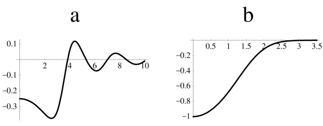
Figure 1: The 2-dimensional vector zero correlation function $g_{2}(r),$ plotted for two choices of $C(r):$ (a) $C(r)=J_{0}(r);$ (b) $C(r)=\exp(-r^{2}/2).$

5 Critical points in two dimensions

In this section, the scheme of section 2 is used to calculate the topological charge correlation function of critical points of isotropic gaussian random functions in the plane, that is the Poincaré index correlation function of isotropic random surfaces.

The gaussian random function examined shall be written $f=f(\bi{r})=f(x,y)$ (where $x=r_{1},y=r_{2}$), which will be assumed stationary and isotropic, so the expressions in section 3 may be used. In particular, $f$ and its first derivatives have the correlations (3.5), (3.6), as well as further correlations involving second derivatives, described below. As in the previous section, for convenience in calculations, the two points $A$ and $B$ are separated only in the $x$ coordinate.

At a critical point, the gradient $\nabla f=(f_{,x},f_{,y})$ is zero. The critical point jacobian $\mathcal{J}_{\mathrm{c}}$ whose sign defines the topological charge (Poincaré index) is the hessian determinant

$$\mathcal{J}_{\mathrm{c}}=\det f_{,ij}=f_{,xx}f_{,yy}-f_{,xy}^{2};$$ (5.1)

this is the gaussian curvature of the surface. Unlike a general 2-dimensional random vector field (as in the previous section), the gradient field $\nabla f$ is irrotational, which gives rise to relationships and correlations between the derivatives of the components (e.g. $f_{,xy}=f_{,yx}$, whereas before, $v_{1,2}\neq v_{2,1}$ in general). This makes the explicit computation of the topological charge correlation function more difficult than in the previous section, even in the 2-dimensional case that is considered here; the scheme of section 2 applies to gradient zeros in fields of any dimension.

The statistical properties of critical points of gaussian random fields in 2 dimensions were considered by Longuet-Higgins (1957a,b); he found that the density $d_{\mathrm{c}}$ of critical points is (Longuet-Higgins 1957b equations (71), (78)):

$$d_{\mathrm{c}}=\left|\frac{2C^{(4)}_{0}}{3\pi\sqrt{3}C^{\prime\prime}_{0}}\right|,$$ (5.2)

($C^{(4)}_{0}$ denotes the fourth derivative of $C,$ evaluated at $r=0$). The density of saddles equals the density of extrema (maxima and minima), and the density of maxima equals the density of minima. The probability density function of the gaussian curvature $\mathcal{J}$, despite its asymmetry (Longuet-Higgins 1958 equation (7.14), Dennis 2002 equation (57)), has zero first moment, implying the average topological charge $\langle\delta^{2}(\nabla f)\mathcal{J}_{\mathrm{c}}\rangle$ is zero, as expected.

The topological charge correlation function is again calculated using the scheme of section 2, particularly (2.10). Therefore, the vector $\bi{u}$ (2.3) of gaussian random variables, in a convenient ordering, is

$$\bi{u}_{\mathrm{c}}=(f_{A,xx},f_{A,yy},f_{B,xx},f_{B,yy},f_{A,xy},f_{B,xy},f_{A,x},f_{B,x},f_{A,y},f_{B,y})$$ (5.3)

with correlation matrix (c.f. (2.2))

$$\boldsymbol{\Sigma}_{\mathrm{c}}=\left(\begin{array}[]{cccccccccc}M_{0}&L_{0}&M&L&0&0&0&G&0&0\\ L_{0}&M_{0}&L&N&0&0&0&I&0&0\\ M&L&M_{0}&L_{0}&0&0&-G&0&0&0\\ L&N&L_{0}&M_{0}&0&0&-I&0&0&0\\ 0&0&0&0&L_{0}&L&0&0&0&I\\ 0&0&0&0&L&L_{0}&0&0&-I&0\\ 0&0&-G&-I&0&0&F_{0}&F&0&0\\ G&I&0&0&0&0&F&F_{0}&0&0\\ 0&0&0&0&0&-I&0&0&F_{0}&H\\ 0&0&0&0&I&0&0&0&H&F_{0}\\ \end{array}\right),$$ (5.4)

where the correlations between elements of $\bi{u}_{\mathrm{c}}$ are computed to be

$$G \equiv\left[\partial_{x}^{3}C\right]_{x=r,y=0} =C^{(3)}$$

$$I \equiv\left[\partial_{x}^{2}\partial_{y}C\right]_{x=r,y=0} =(rC^{\prime\prime}-C^{\prime})/r^{2}$$

$$L \equiv\left[\partial_{x}^{2}\partial_{y}^{2}C\right]_{x=r,y=0} =(r^{2}C^{(3)}-2rC^{\prime\prime}+2C^{\prime})/r^{3}$$

$$M \equiv\left[\partial_{x}^{4}C\right]_{x=r,y=0} =C^{(4)}$$

$$N \equiv\left[\partial_{y}^{4}C\right]_{x=r,y=0} =3(rC^{\prime\prime}-C^{\prime})/r^{3}$$

$$G_{0} =I_{0}=0, M_{0}=N_{0}=3L_{0}=C^{(4)}_{0}.$$ (5.5)

The last line gives the special value of these correlations when $r=0.$

The matrix $\mathbf{K}_{\mathrm{c}}$ is the $4\times 4$ lower right submatrix of $\boldsymbol{\Sigma}_{\mathrm{c}},$ and has determinant

$$\det\mathbf{K}_{\mathrm{c}}=(F_{0}^{2}-H^{2})(F_{0}^{2}-F^{2}).$$ (5.6)

The pair of differential jacobian operators are, from (5.1),

$$\mathcal{J}_{\nabla A}\mathcal{J}_{\nabla B}=\nabla_{1}\nabla_{2}\nabla_{3}\nabla_{4}+\nabla_{5}^{2}\nabla_{6}^{2}-\nabla_{1}\nabla_{2}\nabla_{6}^{2}-\nabla_{3}\nabla_{4}\nabla_{5}^{2}.$$ (5.7)

Using (2.12), the result of these operators acting is on $\exp(-\bi{t}\cdot\boldsymbol{\Xi}\cdot\bi{t}/2)$ and setting $\bi{t}=\mathbf{0}$ (c.f. (2.10),(2.11)) is

$$D_{\mathrm{c}}=\Xi_{14}\Xi_{23}+\Xi_{13}\Xi_{24}-2\Xi_{16}\Xi_{26}+\Xi_{12}\Xi_{34}-2\Xi_{35}\Xi_{45}-\Xi_{34}\Xi_{55}+2\Xi_{56}^{2}-\Xi_{12}\Xi_{66}+\Xi_{55}\Xi_{66},$$ (5.8)

where the necessary entries of $\boldsymbol{\Xi}_{\mathrm{c}},$ are found using Jacobi’s determinant theorem in (1.5); as an example,

$$\Xi_{24}=M_{0}-FI^{2}/(F_{0}^{2}-F^{2}).$$ (5.9)

The topological charge correlation function $g_{\rm{c}}(r)$ for critical points is obtained by substituting (5.6), (5.8) (with all terms like (5.9) found using (1.5) into (2.10)). This expression is complicated and not very illuminating, and is not given here. Upon substituting (3.5), (3.6), (5.5) in, one finds that $g_{\mathrm{c}}$ can be written as a perfect derivative (c.f. (4.8)),

$$g_{\mathrm{c}}(r)=\frac{1}{4\pi^{2}d_{\mathrm{c}}^{2}r}\frac{\rmd h_{\mathrm{c}}}{\rmd r},$$ (5.10)

where

$$h_{\mathrm{c}}(r)=\frac{(C^{\prime\prime}-C^{\prime}/r)}{r\sqrt{(C_{0}^{\prime\prime 2}-C^{\prime\prime 2})(C_{0}^{\prime\prime 2}-C^{\prime 2}/r^{2})}}\left[\frac{C^{(3)}(3C_{0}^{\prime\prime 2}-2C^{\prime\prime 2}-C^{\prime\prime}C^{\prime}/r)}{C_{0}^{\prime\prime 2}-C^{\prime\prime 2}}\right.$$

$$\hbox to0.0pt{\hss${}\quad{}$}\left.-\frac{(C^{\prime\prime}-C^{\prime}/r)(3C_{0}^{\prime\prime 2}-2C^{\prime 2}/r^{2}-C^{\prime\prime}C^{\prime}/r)}{r(C_{0}^{\prime\prime 2}-C^{\prime 2}/r^{2})}\right]$$

$$\hbox to0.0pt{\hss${}={}$}\frac{1}{r(C^{\prime\prime}-C^{\prime}/r)}\frac{\rmd}{\rmd r}\frac{(C^{\prime\prime}-C^{\prime}/r)^{3}}{\sqrt{(C_{0}^{\prime\prime 2}-C^{\prime\prime 2})(C_{0}^{\prime\prime 2}-C^{\prime 2}/r^{2})}}.$$ (5.11)

This process of finding $h_{\mathrm{c}}$ is long and tedious, and details are omitted here. It is easy to see that $h_{\mathrm{c}}\to 0$ as $r\to\infty;$ it is straightforward, by Taylor expanding derivatives of $C,$ to show that

$$h_{\mathrm{c}}(0)=\frac{4C^{(4)}_{0}}{3\sqrt{3}C^{\prime\prime}_{0}}=-2\pi d_{\mathrm{c}}.$$ (5.12)

The critical point topological charge correlation function for two particular field correlation functions is shown in figure 2. As with the 2-dimensional vector case plotted in figure 1, the properties of the correlation function (oscillatory, exponential decay, etc) are similar to that of the underlying field correlation function $C(r),$ on which the correlation function depends. Features of interest in these plots include the sharp initial minimum of (a), and the fact that the monotonic decay in (b) is from above, not below (in contrast to its counterpart in figure 1. Nevertheless, the form of $h_{\mathrm{c}}$ is significantly more complicated than $h_{n},$ especially when $n=2.$

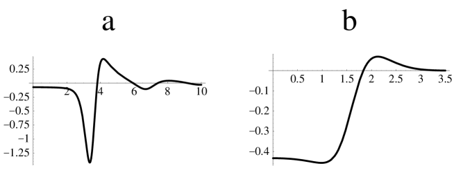
Figure 2: The critical point charge correlation function $g_{\mathbf{c}}(r),$ plotted for two choices of $C(r):$ (a) $C(r)=J_{0}(r);$ (b) $C(r)=\exp(-r^{2}/2).$

6 Umbilic points

Less well-known than critical points, umbilic points are geometric point singularity features associated with the second derivative of $f$ - namely where hessian matrix of second derivatives $\partial_{ij}f$ is degenerate (Berry and Hannay 1977, Porteous 2001, Hilbert and Cohn-Vossen 1952). Geometrically, the principal axes of gaussian curvature are not defined at these points. The eigenvalues of the hessian coincide when $f_{,xx}=f_{,yy},\,f_{,xy}=0.$ Umbilic points are therefore zeros of the 2-dimensional vector field

$$\bi{v}_{\mathrm{u}}=\left((f_{,xx}-f_{,yy})/2,f_{,xy}\right).$$ (6.1)

The factor of half in the first term ensures that $\bi{v}_{\mathrm{u}}$ is statistically rotation invariant.

An umbilic point has an index, determined geometrically by the sense of rotation of the principal axes of curvature around the umbilic point, and the index is generically $\pm 1/2$ (Berry and Hannay 1977); only the sign of the index is of interest here, and this is determined by the appropriate jacobian $\mathcal{J}_{\mathrm{u}}$ on $\bi{v}_{\mathrm{u}}$,

$$2\mathcal{J}_{\mathrm{u}}=f_{,xxx}f_{,xyy}+f_{,yyy}f_{,xxy}-f_{,xyy}^{2}-f_{,xxy}^{2},$$ (6.2)

depending on the third partial derivatives of $f.$ The calculation of the topological charge correlation function for umbilic points can proceed according to the scheme of section 2, in a similar way to the corresponding calculation for critical points.

Umbilic points for isotropic random functions was considered by Berry and Hannay; they found the density $d_{\mathrm{u}}$ to be (Berry and Hannay 1977 equation (34))

$$d_{\mathrm{u}}=\left|\frac{3C^{(6)}_{0}}{10\pi C^{(4)}_{0}}\right|,$$ (6.3)

($C^{(6)}_{0}$ is the sixth derivative of $C$ at 0) and that the average index $q$ is zero (the separate densities are $0.5d_{\mathrm{u}}$ for stars, $0.05279d_{\mathrm{u}}$ for monstars, and $0.44721d_{\mathrm{u}}$ for lemons). In the present work, the distinction between monstars and lemons, which both have positive index, is not used.

The ordering of the vector of gaussian random functions $\bi{u}_{\mathrm{u}}$ is chosen

$$\bi{u}_{\mathrm{u}}=(f_{A,xxx},f_{A,xyy},f_{B,xxx},f_{B,xyy},f_{A,xxy},f_{A,yyy},f_{B,xxy},f_{B,yyy},$$

$$\qquad\qquad(f_{A,xx}-f_{A,yy})/2,(f_{B,xx}-f_{B,yy})/2,f_{A,xy},f_{B,xy}).$$ (6.4)

The correlation matrix (2.2) is

$$\boldsymbol{\Sigma}_{\mathrm{u}}=\left(\begin{array}[]{cccccccccccc}S_{0}&T_{0}&S&T&0&0&0&0&0&-X&0&0\\ T_{0}&T_{0}&T&U&0&0&0&0&0&-Y&0&0\\ S&T&S_{0}&T_{0}&0&0&0&0&X&0&0&0\\ T&U&T_{0}&T_{0}&0&0&0&0&Y&0&0&0\\ 0&0&0&0&T_{0}&T_{0}&T&U&0&0&0&-Q\\ 0&0&0&0&T_{0}&S_{0}&U&V&0&0&0&-R\\ 0&0&0&0&T&U&T_{0}&T_{0}&0&0&Q&0\\ 0&0&0&0&U&V&T_{0}&S_{0}&0&0&R&0\\ 0&0&X&Y&0&0&0&0&L_{0}&W&0&0\\ -X&-Y&0&0&0&0&0&0&W&L_{0}&0&0\\ 0&0&0&0&0&0&Q&R&0&0&L_{0}&L\\ 0&0&0&0&-Q&-R&0&0&0&0&L&L_{0}\\ \end{array}\right),$$ (6.5)

where $W\equiv(M+N-2L)/4,X\equiv(P-Q)/2,Y\equiv(Q-R)/2,$ and

$$P \equiv-\left[\partial_{x}^{5}C\right]_{x=r,y=0} =-C^{(5)},$$

$$Q \equiv-\left[\partial_{x}^{3}\partial_{y}^{2}C\right]_{x=r,y=0} =-(r^{3}C^{(4)}-3r^{2}C^{(3)}+6rC^{\prime\prime}-6C^{\prime})/r^{4},$$

$$R \equiv-\left[\partial_{x}\partial_{y}^{4}C\right]_{x=r,y=0} =-3(r^{2}C^{(3)}-3rC^{\prime\prime}+3C^{\prime})/r^{4},$$

$$S \equiv-\left[\partial_{x}^{6}C\right]_{x=r,y=0} =-C^{(6)},$$

$$T \equiv-\left[\partial_{x}^{4}\partial_{y}^{2}C\right]_{x=r,y=0} =-(r^{4}C^{(5)}-4r^{3}C^{(4)}+12r^{2}C^{(3)}-24rC^{\prime\prime}+24C^{\prime})/r^{5},$$

$$U \equiv-\left[\partial_{x}^{2}\partial_{y}^{4}C\right]_{x=r,y=0} =-3(r^{3}C^{(4)}-5r^{2}C^{(3)}+12rC^{\prime\prime}-12C^{\prime})/r^{5},$$

$$V \equiv-\left[\partial_{y}^{6}C\right]_{x=r,y=0} =-15(r^{2}C^{(3)}-3rC^{\prime\prime}+3C^{\prime})/r^{5},$$

$$P_{0} =Q_{0}=R_{0}=0, S_{0}=5T_{0}=5U_{0}=V_{0}=-C^{(6)}_{0}.$$ (6.6)

The matrix $\mathbf{K}_{\mathrm{u}},$ defined using (2.5), has determinant

$$\det\mathbf{K}_{\mathrm{u}}=(L_{0}^{2}-(M+N-2L)^{2}/16)(L_{0}^{2}-L^{2}).$$ (6.7)

The result of the jacobian derivative operators (2.11) gives

$$D_{\mathrm{u}}=\Xi_{12}^{2}+\Xi_{14}^{2}+\Xi_{22}^{2}+2\Xi_{24}^{2}-2\Xi_{12}\Xi_{22}+\Xi_{13}\Xi_{24}-4\Xi_{14}\Xi_{24}-2\Xi_{12}\Xi_{55}+2\Xi_{12}\Xi_{56}$$

$$-2\Xi_{22}\Xi_{56}+\Xi_{55}^{2}+\Xi_{56}^{2}+2\Xi_{57}^{2}+\Xi_{58}^{2}-2\Xi_{55}\Xi_{56}-4\Xi_{57}\Xi_{58}+\Xi_{57}\Xi_{68}.$$ (6.8)

The necessary entries of $\boldsymbol{\Xi}_{\mathrm{u}}$ are found using (1.5). The resulting expression for $D_{\mathrm{u}},$ and therefore for $g_{\mathrm{u}},$ is very complicated, but may be reduced to the following form:

$$g_{\mathrm{u}}(r)=\frac{1}{4\pi^{2}d_{\mathrm{u}}^{2}r}\frac{\rmd h_{\mathrm{u}}}{\rmd r},$$ (6.9)

where

$$h_{\mathrm{u}}(r)=\frac{\rmd}{\rmd r}\left(\frac{r(Q-R)^{2}}{4\sqrt{\det\mathbf{K}_{\mathrm{u}}}}\right)+\frac{Q(P+R-2Q)}{4\sqrt{\det\mathbf{K}_{\mathrm{u}}}}.$$ (6.10)

It can be shown that $h_{\mathrm{u}}(0)=-2\pi d_{\mathrm{u}},$ and $h\to 0$ as $r\to\infty.$ $g_{\mathrm{u}}(r)$ is plotted in figure 3 for $C(r)=J_{0}(r)$ and $\exp(-r^{2}/2).$ The most obvious feature of these two plots, compared to figures 1, 2, is that they have a negative maximum, a property that seems to be general for $g_{\mathrm{u}},$ although this has not been proved. It is unclear what the physical significance of this kink should be; mathematically, it probably arises from interference between the two summands in $h_{\mathrm{u}}(r)$ in (6.10).

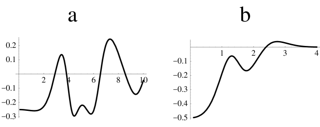
Figure 3: The umbilic charge correlation function $g_{\mathbf{u}}(r),$ plotted for two choices of $C(r):$ (a) $C(r)=J_{0}(r);$ (b) $C(r)=\exp(-r^{2}/2).$

7 Topological charge screening

Three particular charge correlation functions have been derived exactly (equations (4.8), (4.9), (5.10), (5.11), (6.9),(6.10)). In each case, the charge correlation function has the form

$$g(r)=\frac{(n-1)!}{(2\pi)^{n}d^{2}r^{n-1}}\frac{\rmd h(r)}{\rmd r},$$ (7.1)

where $n$ is the number of dimensions, $d$ is the density of zeros and $h(r)$ is a function such that

$$h(0)=\frac{(2\pi)^{n}d}{\sigma_{n-1}(n-1)!},\qquad h\to\infty\mathrm{\,as\,}r\to\infty.$$ (7.2)

The total charge density around a given (say positive) topological charge is therefore

$$d\int\rmd^{n}\bi{r}\,g(r) = \frac{(n-1)!}{(2\pi)^{n}d}\sigma_{n-1}\int_{0}^{\infty}\rmd r\,\frac{\rmd h(r)}{\rmd r}$$ (7.3)

$$= \frac{(n-1)!\sigma_{n-1}}{(2\pi)^{n}d^{2}}(h(\infty)-h(0))$$

$$= -1,$$

where the hypersphere area $\sigma_{n-1}$ appears in the first line from integration in polar coordinates. It implies that the distribution of topological charges is such that every topological charge tends to be surrounded by charges of the opposite sign, such that the topological charge is ‘screened’ at large distances. This fact was noticed in the random vector case by Halperin (1981) and Liu and Mazenko (1992) (although the general zero density $d_{n}$ had not been determined explicitly) and is independent of the field correlation function $C.$ The derivation here shows that this is a more general phenomenon, possibly a universal feature of topological charge correlations for gaussian random fields. It should be noted that (7.3) is not necessarily satisfied for an arbitrary distribution of signed points; for instance, $g(r)=0$ always for Poisson points, for which there is no screening. $\delta$-function correlations at the origin are ignored in the following.

An analogy may be drawn from the theory of ionic liquids (Hansen and McDonald 1986); in a fluid or plasma, consisting of two species identical except for opposite (Coulomb) charges, the following Stillinger-Lovett sum rules (Stillinger and Lovett 1968a,b) are found to hold:

$$d\int\rmd^{n}\bi{r}\,g(r) = -1,$$ (7.4)

$$d\int\rmd^{n}\bi{r}\,r^{2}g(r) = -a_{n}\Lambda^{2}.$$ (7.5)

Here, $g$ is the charge-charge correlation function, $\Lambda$ is a characteristic screening length dependent on temperature and $n,$ and $a_{n}$ is a constant dependent on dimensionality. These rules are discussed for $n=3$ by Hansen and McDonald (1986), Stillinger and Lovett 1968a,b, and $n=2$ by Jancovici 1987, Jancovici et al1994.

The screening relation (7.3) is equivalent to the first Stillinger-Lovett sum rule (7.4), which is derived using the statistical mechanics of pairwise, Coulomb interacting fluids. It is unclear whether the fact that topological and coulombic charges screen in the same way is coincidence, or evidence of some deeper connection between the two statistical theories.

It is natural to ask whether the topological charge correlation functions satisfy the second sum rule, which (upon integrating the left hand side of (7.5) by parts), depends on the integral of $rh.$ For $n=2,$ it was found (Berry and Dennis 2000) that for certain choices of $C,$ this integral may diverge. The slowest decay comes when $C=J_{0},$ and by (4.9),

$$h_{2}(r)\sim_{r\to\infty}\cos(r+\pi/4)^{2}/r\qquad\mathrm{when}\quad C=J_{0},$$ (7.6)

giving a logarithmic divergence for the second moment. For comparison, the critical and umbilic functions $h_{\mathrm{c}},h_{\mathrm{u}},$ (equations (5.11), (6.10) respectively) both give, for the same choice of $C,$

$$h_{\mathrm{c}}(r),h_{\mathrm{u}}(r)\sim_{r\to\infty}\cos(2r)/r^{2}\qquad\mathrm{when}\quad C=J_{0},$$ (7.7)

implying that the second sum rule is satisfied generally for critical and umbilic points, although, as for the cases of random vectors where the integral converges, the screening length $\Lambda,$ defined in analogy to (7.5), depends on the choice of $C.$ For random vectors with $n>2,$ the second moment of $g$ always converges, because of the higher power of $C^{\prime}$ appearing in (4.9) (also, the decay of $C$ will be faster, as discussed at the end of section 3).

Comparison may be drawn to the electrostatic analogy in random matrix theory, particularly in the case of the so-called Ginibre ensemble of $N\times N$ matrices whose entries are independent, identically distributed circular gaussian random variables (Ginibre 1965). The eigenvalues of these matrices are found to have exactly the same statistical behaviour as a 1-component 2-dimensional Coulomb gas of $N$ charges in a harmonic oscillator potential, and the 2-point density correlation function screens against a uniform background (i.e. $d\int\rmd^{2}z\,(g_{\mathrm{Gin}}-1)=-1$), and have finite second moment. Certain random polynomial analogues have zeros that can also be expressed as 2-dimensional Coulomb gases with additional interactions (Hannay 1998, Forrester and Honner 1999). The eigenvalues of random matrices (which may be expressed as the zeros of the characteristic polynomial) and zeros of random polynomials are all of the same sign, since they are zeros of complex analytic functions, and the density correlation functions of zeros are unique (there is no analogue of $C$).

There may be a danger in taking the analogy with fluids too far; for instance, the oscillations of the functions in figures 1,2,3a are reminiscent of those of charged fluids (e.g. Hansen and McDonald 1986). However, the physical causes for these oscillations are very different. In fluids, the oscillations usually arise from packing considerations (the ions themselves are of finite size, fixing the lengthscale, although in plasmas they are usually represented as point charges (Baus and Hansen 1980)). Topological charges, on the other hand, are points, and the oscillations in these figures originate from the oscillations in the underlying field correlation function $C(r),$ which is $J_{0}$ in this case. Although Halperin (1981) discusses the similarity between the short-range behaviour of the 2-dimensional vector correlation function (4.8), (4.9) and Kosterlitz-Thouless theory, the present situation is more general, both in that the (possibly long-range) screening is exact, and that the results hold for any reasonable field correlation function $C(r).$

8 Discussion

Using a general scheme for calculating topological charge correlation functions, three particular correlation functions were found explicitly, and were found always to satisfy a screening relation (7.3).

The scheme of section 2 used to calculate the charge correlation functions is very general, and can be generalised to calculate the charge-charge correlation function between two different sets of topological charges - for instance with a critical point at $A,$ and an umbilic point at $B.$ Although not done so here, the scheme may be applied to anisotropic fields.

It is rather more difficult to calculate the density correlation function for topological charges (the analogue of (1.3) where the moduli of the jacobians are taken). It was calculated for 1-dimensional vectors (i.e. random functions in 1 dimension) by Rice (1954), and for 2-dimensional vectors (realised as complex scalars) by Berry and Dennis (2000), Saichev et al(2001). However, it has not been possible to generalise such methods to the case of critical points. Also, numerical evidence (Freund and Wilkinson 1998) suggests that the correlation function of extrema signed by the sign of their laplacian ($+1$ for minima, $-1$ for maxima) also satisfies the screening relation (7.4). All such functions would be needed to calculate the partial correlation functions between the species (e.g. maxima with maxima, maxima with saddles, maxima with minima, etc), which would give a complete statistical picture.

The presence of boundaries in the random function will affect the statistical properties of topological charges (e.g. Berry (2002) for nodal points in the plane), and it is possible that there may be some further analogy with the physics of interfaces of Coulomb fluids. The scheme of section 2 ought to be adaptable to calculate charge correlation functions in this case.

Only zeros of fields linear in gaussian random functions have been considered here, although the density of others may be calculated, for instance, in addition to nodal points, a 2-dimensional gaussian random complex scalar has critical points of its modulus squared (Weinrib and Halperin 1982) and its argument (Dennis 2001a). The scheme employed here cannot be used to calculate correlation functions for these, although numerical evidence (I Freund, personal communication) suggests that the critical points of argument (together with the nodal points) do screen, therefore adding to the cases shown here. It is tempting to conjecture that topological charge screening may be a universal phenomenon in gaussian random fields.

Appendix A Jacobi’s determinant theorem

Let $\mathbf{A}$ be a square matrix. The minor $\mathcal{M}^{i_{1}\dots i_{k}}_{j_{1}\dots j_{k}}(\mathbf{A})$ is the determinant of the $k\times k$ submatrix of $\mathbf{A}$ with rows $i_{1},\dots,i_{k}$ and columns $j_{1},\dots,j_{k}.$ $\overline{\mathcal{M}}^{i_{1},\dots,i_{k}}_{j_{1},\dots,j_{k}}(\mathbf{A})$ shall be used to denote the complementary minor, that is, the minor of the submatrix of $\mathbf{A}$ with rows $i_{1},\dots,i_{k}$ and columns $j_{1},\dots,j_{n}$ excluded. Then Jacobi’s determinant theorem (Jeffreys and Jeffreys 1956, page 135) states

$$\det\mathbf{A}\,\mathcal{M}^{i_{1},\dots,i_{k}}_{j_{1},\dots,j_{k}}(\mathbf{A}^{-1})=(-1)^{i_{1}+\dots+i_{k}+j_{1}+\dots+j_{k}}\overline{\mathcal{M}}^{i_{1},\dots,i_{k}}_{j_{1},\dots,j_{k}}(\mathbf{A}).$$ (1.1)

Applying this to $\boldsymbol{\Sigma}$ in (2.5), and choosing $\boldsymbol{\Xi}^{-1}$ as the submatrix whose determinant is the minor of $\boldsymbol{\Sigma}^{-1},$

$$\det\boldsymbol{\Sigma}\,\det\boldsymbol{\Xi}^{-1} = \det\boldsymbol{\Sigma}\,\mathcal{M}^{1,\dots,2m}_{1,\dots,2m}(\boldsymbol{\Sigma}^{-1})$$ (1.2)

$$= (-1)^{1+\dots+2m+1+\dots+2m}\mathcal{M}^{2m+1,\dots,2(m+n)}_{2m+1,\dots,2(m+n)}(\boldsymbol{\Sigma})$$

$$= \det\mathbf{K},$$

from which (2.6) follows directly.

Jacobi’s theorem can also be used to find the elements $\Xi_{ij}$ of the inverse reduced inverse matrix $\boldsymbol{\Xi}$ in (2.5), needed for (2.12). In this case, (1.1) is applied twice, once on the matrix $\boldsymbol{\Xi}^{-1},$ and once on $\boldsymbol{\Sigma}.$ Therefore

$$\Xi_{ij} = \mathcal{M}^{i}_{j}(\boldsymbol{\Xi})$$ (1.5)

$$= (-1)^{i+j}\overline{\mathcal{M}}^{i}_{j}(\boldsymbol{\Xi}^{-1})/\det\boldsymbol{\Xi}^{-1}$$

$$= (-1)^{i+j}\det{\boldsymbol{\Xi}}\,\mathcal{M}^{1,\dots,i-1,i+1,\dots,2m}_{1,\dots,j-1,j+1,\dots,2m}(\boldsymbol{\Sigma}^{-1})$$

$$= \det{\boldsymbol{\Xi}}\,\mathcal{M}^{i,2m+1,\dots,2m+2n}_{j,2m+1,\dots,2m+2n}(\boldsymbol{\Sigma})$$

$$= \mathcal{M}^{i,2m+1,\dots,2m+2n)}_{j,2m+1,\dots,2m+2n}(\boldsymbol{\Sigma})/\det\mathbf{K},$$

$$= \det\mathbf{K}^{-1}\det\left(\begin{array}[]{cc}\Sigma_{ij}&\bullet\\ \bullet&\mathbf{K}\end{array}\right)$$

where in the last line $\bullet$ represents the terms $\Sigma_{i,k},\Sigma_{k,j}$ where $k=2m+1,\dots,2m+2n.$ Thus the $\Xi_{ij}$ appearing in the expression for $D$ in (2.12), is the determinant of the $(2n+1)\times(2n+1)$ submatrix comprised of the $i$th row and $j$th column of $\boldsymbol{\Sigma},$ and the submatrix $\mathbf{K}.$

Appendix B Calculation of the density of vector zeros (4.1)

In order to integrate (4.1), the following must be integrated

$$\mathcal{V}=\int\rmd^{n^{2}}v_{i,j}\,|\det v_{i,j}|\exp\left(-\frac{1}{2}\sum_{i,j=1}^{n}v_{i,j}^{2}\right).$$ (2.1)

This is, mathematically, the average hypervolume of an $n$-dimensional parallelepiped specified by gaussian random vectors $\bi{w}_{1}=(v_{1,1},\dots v_{1,n}),\dots,\bi{w}_{n}=(v_{n,1},\dots,v_{n,n}).$ These gaussian random vectors are identically distributed isotropically in $n$-dimensional space. The hypervolume is nonzero exactly when the set of $n$ vectors is linearly independent.

This hypervolume may be found explicitly in a manner reminiscent of the Gram-Schmidt orthogonalization procedure for vectors. Geometrically,

$$\rm{volume\,of\,parallelepiped}=\rm{length\,of\,}\bi{w}_{1}\times\rm{\,length\,of\,}\bi{w}_{2}\rm{\,orthogonal\,to\,}\bi{w}_{1}\times\dots$$

$$\times\rm{\,length\,of\,}\bi{w}_{n}{\,\rm orthogonal\,to\,}\mathrm{span}\{\bi{w}_{1},\dots,\bi{w}_{n-1}\}.$$ (2.2)

A given factor in this product is therefore the average length of the gaussian random vector $\bi{w}_{j}$ in the orthogonal complement of a $(j-1)$-dimensional subspace $\mathrm{span}\{\bi{w}_{1},\dots,\bi{w}_{j-1}\}.$

Now, since the vector $\bi{w}_{j}$ is isotropic, it may be represented identically in any choice of orthonormal basis of $n$-dimensional space; in particular, its first $j-1$ components $v_{j,1},\dots,v_{j,j-1}$ may be chosen to be in $\mathrm{span}\{\bi{w}_{1},\dots,\bi{w}_{j-1}\}$ (as in the Gram-Schmidt procedure). The total contribution of $\bi{w}_{j}$ to the integral in (4.1) involves the average length of the vector made up of the other components $v_{j,j},\dots,v_{j,n}.$ Where $k=n-j-1,$ this is

$$\int\rmd^{n}\bi{w}_{j}\,\sqrt{v_{j,1}^{2}+\dots+v_{j,n}^{2}}\exp\left(-\frac{1}{2}\sum_{i=1}^{n}v_{j,i}^{2}\right)$$

$$=\left[\int_{-\infty}^{\infty}\rmd v_{j,1}\,\exp(-v_{j,1}^{2}/2)\right]^{j-1}\int_{\mathcal{S}_{k-1}}\rmd^{k-1}\Omega_{k-1}\int_{0}^{\infty}\rmd\rho\,\rho^{k}\exp(-\rho^{2}/2)$$ (2.3)

where, in the second line, the first $m-1$ components have been pulled out as trivial gaussians, integrating to $(2\pi)^{(j-1)/2}=(2\pi)^{(n-k)/2};$ the remaining $k$ integrals are the average length of a gaussian random vector in $k$-dimensional space. This integral has been converted to polar coordinates, with $\rmd\omega_{k-1}$ the solid angle infinitesimal on the unit $(k-1)$-sphere $\mathcal{S}_{k-1},$ and $\rho$ is the radius. It is well known that the surface area $\sigma_{k-1}$ of the unit $(k-1)$-hypersphere is

$$\sigma_{k-1}=\int\rmd^{k-1}\Omega_{k-1}=\frac{2\pi^{k/2}}{(\frac{k-2}{2})!}.$$ (2.4)

The $\rho$ integral in (2.3) is $2^{(k-1)/2}((k-1)/2)!.$ Therefore, the numerical part of (4.1) is $1/(2\pi)^{n(n+1)/2}$ times the product in (2.2), with each term in the product, now labelled by $k,$ given by the expression (2.3). Therefore

$$\mathcal{V} = \frac{1}{(2\pi)^{n(n+1)/2}}\prod_{k=1}^{n}(2\pi)^{(n-k)/2}\times\frac{2\pi^{k/2}}{(\frac{k-2}{2})!}\times 2^{(k-1)/2}\left(\frac{k-1}{2}\right)!$$ (2.5)

$$= \frac{1}{(2\pi)^{n(n+1)/2}}\prod_{k=1}^{n}(2\pi)^{(n+1)/2}\pi^{n/2}\frac{(\frac{k-1}{2})!}{(\frac{k-2}{2})!}$$

$$= \frac{(\frac{n-1}{2})!}{\pi^{(n+1)/2}}.$$

This value agrees with that stated by Halperin (1981), Liu and Mazenko (1992) of $1/\pi$ ($n=1$), $1/2\pi$ ($n=2$) and $1/\pi^{2}$ ($n=3$).

References

References

- [1]
- [2] [] Adler R J 1981 The geometry of random fields (Wiley)
- [3]
- [4] [] Baus M and Hansen J-P 1980 Statistical mechanics of simple Coulomb systems Phys.Rep. 59 1–94
- [5]
- [6] [] Berry M V 1977 Regular and irregular semiclassical wavefunctions J.Phys.A:Math.Gen. 10 2083–91
- [7]
- [8] [] —–1978 Disruption of wavefronts: statistics of dislocations in incoherent gaussian random waves J.Phys.A:Math.Gen. 11 27–37
- [9]
- [10] [] —–2002 Statistics of nodal lines and points in quantum billiards: perimeter corrections, fluctuations, curvature J.Phys.A:Math.Gen. 35 3025–38
- [11]
- [12] [] Berry M V and Hannay J H 1977 Umbilic points on a gaussian random surface J.Phys.A:Math.Gen. 10 1809–21
- [13]
- [14] [] Berry M V and Dennis M R 2000 Phase singularities in isotropic random waves Proc.R.Soc.Lond.A. 456 2059–79 (errata 456 3059).
- [15]
- [16] [] Dennis M R 2001a Phase critical point densities in planar isotropic random waves J.Phys.A:Math.Gen. 34 L297–L303
- [17]
- [18] [] —–2001b Topological singularities in wave fields Ph.D. thesis, Bristol University
- [19]
- [20] [] —–2002 Polarization singularities in paraxial vector fields: morphology and statistics Opt.Commun. 213 201–21
- [21]
- [22] [] Feller W 1950 An introduction to probability theory and its applications, volume I. (Wiley, New York)
- [23]
- [24] [] Foltin G 2003a Signed zeros of gaussian vector fields - density, correlation functions and curvature J.Phys.A:Math.Gen. 36 1729–41
- [25]
- [26] [] —–2003b The distribution of extremal points of Gaussian scalar fields. J.Phys.A:Math.Gen. 36 4561–80
- [27]
- [28] [] Forrester P J and Honner G 1999 Exact statistical properties of complex random polynomials J.Phys.A:Math.Gen. 32 2961–81
- [29]
- [30] [] Freund I and Wilkinson M 1998 Critical-point screening in random wave fields J.Opt.Soc.Am.A 15 2892–902
- [31]
- [32] [] Ginibre J 1965 Statistical ensembles of complex, quaternion and real matrices. J.Math.Phys. 6 440–49
- [33]
- [34] [] Halperin B I 1981 Statistical mechanics of topological defects. in R Balian, M Kléman, and J-P Poirier, eds, Les Houches Session XXV - Physics of Defects (North-Holland, Amsterdam)
- [35]
- [36] [] Hannay J H 1998 The chaotic analytic function J.Phys.A:Math.Gen. 31 L755–61
- [37]
- [38] [] Hansen J-P and McDonald I R 1986 Theory of simple liquids (Academic Press)
- [39]
- [40] [] Hilbert D and Cohn-Vossen S 1952 Geometry and the Imagination (Chelsea Publishing)
- [41]
- [42] [] Jancovici B 1987 Charge correlations and sum rules in Coulomb systems. I. in F J Rogers and H E Dewitt, eds, Strongly Coupled Plasma Physics (Plenum)
- [43]
- [44] [] Jancovici B, Manificat G and Pisani C 1994 Coulomb systems seen as critical systems: Finite-size effects in two dimensions J.Stat.Phys. 78 307–29
- [45]
- [46] [] Jeffreys H and Jeffreys B S 1956 Methods of Mathematical Physics (Cambridge University Press)
- [47]
- [48] [] Liu F and Mazenko G F 1992 Defect-defect correlation in the dynamics of first-order phase transitions Phys.Rev.B 46 5963–71
- [49]
- [50] [] Longuet-Higgins M S 1957a The statistical analysis of a random, moving surface Phil.Trans.R.Soc.A, 249 321–87
- [51]
- [52] [] —–1957b Statistical properties of an isotropic random surface Phil.Trans.R.Soc.A 250 157–74
- [53]
- [54] [] —–1958 The statistical distribution of the curvature of a random Gaussian surface Proc.Camb.Phil.Soc. 54 439–53
- [55]
- [56] [] Mermin N D 1979 The topological theory of defects in ordered media Rev.Mod.Phys. 51 591–648
- [57]
- [58] [] Milnor J W 1965 Topology from the differentiable viewpoint (Virginia University Press)
- [59]
- [60] [] Nye J F and Berry M V 1974 Dislocations in wave trains Proc.R.Soc.Lond.A 336 165–90
- [61]
- [62] [] Porteous I R 2001 Geometric differentiation: for the intelligence of curves and surfaces, 2nd ed (Cambridge University Press)
- [63]
- [64] [] Rice S O Mathematical analysis of random noise, reprinted in N Wax, ed, 1954 Selected papers on noise and stochastic processes (Dover, New York)
- [65]
- [66] [] Saichev A I, Berggren K-F, and Sadreev A F 2001 Distribution of nearest distances between nodal points for the Berry function in two dimensions. Phys.Rev.E 64 036222
- [67]
- [68] [] Stillinger F H and Lovett R 1968a Ion-pair theory of concentrated electrolytes. I. Basic concepts. J.Chem.Phys. 48 3858–68
- [69]
- [70] [] —–1968b General restriction on the distribution of ions in electrolytes J.Chem.Phys. 49 1991–4
- [71]
- [72] [] Weinrib A and Halperin B I 1982 Distribution of maxima, minima, and saddle points of the intensity of laser speckle patterns Phys.Rev.B 26 1362–8
- [73]