Conformal restriction, highest-weight representations and SLE

Abstract

We show how to relate Schramm-Loewner Evolutions (SLE) to highest-weight representations of infinite-dimensional Lie algebras that are singular at level two, using the conformal restriction properties studied by Lawler, Schramm and Werner in [33]. This confirms the prediction from conformal field theory that two-dimensional critical systems are related to degenerate representations.

1 Introduction

The goal of this paper is to show how the Schramm-Loewner evolutions (or Stochastic Loewner Evolutions, which is anyway abbreviated by SLE) can be used to interpret in a simple and elementary way some of the starting points of conformal field theory, stated by Belavin-Polyakov-Zamolodchikov in their seminal paper [7]. In particular, we will see how restriction properties studied in [33] can be rephrased in terms of highest-weight representations of the Lie algebra $\cal A$ of vector fields on the unit circle (and its central extension, the Virasoro algebra). The results in this paper were announced in the note [18].

It is probably worthwhile to spend some lines outlining our perception of the history of this subject (see also the recent review paper by Cardy [10]): It has been recognized by physicists some decades ago that two-dimensional systems from statistical physics near their critical temperatures have some universal features. In particular, some quantities (correlation length for instance) obey universal power laws near the critical temperature, and the value of the (critical) exponent in fact depends only on the phenomenological features of the discrete system (for instance, it is the same for the same model, taken on different lattices). In order to identify the value of the exponents, two techniques turned out to be very successful. The first one is the “Coulomb gas approach” (see e.g. [37] and the references therein, as well as the reprinted papers in [21]), which is based on explicit computations for some specific models. The second one (see Polyakov [38], Belavin-Polyakov-Zamolodchikov [7], Cardy [8]) is conformal field theory. Based on the analogy with some other problems, it is argued in [7] that two-dimensional critical systems are associated to conformal fields. These fields should then satisfy certain relations, such as the Ward identities, which then allow to make a link with highest-weight representations of the Virasoro algebra. Then the critical exponents can be identified from the corresponding highest weights.

We now quote from [22]: “The remarkable link between the theory of highest-weight modules over the Virasoro algebra and conformal field theory and statistical mechanics was discovered by Belavin-Polyakov-Zamolodchikov [6, 7]. Conformal Field Theory has now become a huge field with ramifications to other fields of mathematics and mathematical physics”. We refer for instance to the introduction of [16] and the compilation of papers in [19, 21]. This approach has then been used to develop the related “quantum gravity” method (see e.g. [13]) and the references therein.

It is worthwhile to stress some points: The actual mathematical meaning, intuition or definition of these fields (and their properties, such as the Ward identities) in terms of the discrete two-dimensional models was to our knowledge never clarified. Also, the notion of “conformal invariance” itself for these systems remained rather obscure. In the case of critical percolation, Aizenman [2] formulated clearly what it should mean, but for other famous models such as self-avoiding walks, or Ising, the precise conjecture was never stated until recently.

In [9], Cardy pointed out that in the case of critical percolation, the arguments from [7, 8] could be used in order to predict the exact formula for asymptotic crossing probabilities of a topological rectangle by a percolation cluster. This prediction was popularized in the mathematical community through the review paper by Langlands-Pouliot-StAubin [25], that attracted many mathematicians to this specific problem (including Stas Smirnov). In that paper, the authors also explain how difficult it is for mathematicians to understand Cardy’s arguments.

On a rigorous mathematical level, only limited progress towards the understanding of 2D critical phenomena had been made before the late 90’s. In 1999, Oded Schramm [40] defined a one-parameter family of random curves based on Loewner’s differential equation, SLE_κ indexed by the positive real parameter $\kappa$. These random curves are the only ones which combine conformal invariance and a Markovian-type property (which is usually already satisfied in the discrete setting). Provided that the scaling limit of an interface in a model studied in statistical physics (such as Ising, Potts or percolation) exists and is conformally invariant (and this approach allows one to give a precise meaning to this), then the limiting object must be one of the SLE_κ curves. Conformal invariance has now been rigorously shown in some cases (critical site percolation on the triangular lattice has been solved by Stas Smirnov [42], the case of loop-erased random walks and uniform spanning trees is treated in Lawler-Schramm-Werner [31]). For a general discussion of the conjectured relation between the discrete models and SLE, see [39]. See also [32] for self-avoiding walks and self-avoiding polygons.

In the SLE setting, the critical exponents simply correspond to principal eigenvalues of some differential operators, see Lawler-Schramm-Werner [27, 28, 29, 30]. Recognizing this led to complete mathematical derivations of the values of critical exponents for the models, that have been proved to be conformally invariant, in particular for critical percolation on the triangular lattice (see [43]). In order to establish rigorously the conjectures for the other models, the missing step is to show their conformal invariance.

Using the Markovian property (which implies that with “time” the conditional probabilities of macroscopic events are martingales) of SLE and Itô’s formula, one readily sees that the probabilities of macroscopic events such as crossing probabilities have to satisfy some second order differential equations [27, 28, 29, 41]. This enables one to recover Cardy’s formula in the case of SLE₆, and to generalize it to other models (i.e. for other values of $\kappa$). Note that just as observed by Carleson in the case of critical percolation, these crossing probabilities formulae become extremely simple in well-chosen triangles, as pointed out by Dubédat [11].

It is therefore natural to think that SLE should be related to conformal field theory and to highest-weight representations of the Virasoro Algebra. Bauer-Bernard [3, 4] recently viewed (with a physics approach) SLE as a process living on a “Virasoro group”, which shows such a link and enables them among other things to recover in conformal field theory language, the generalized crossing probabilities mentioned above.

Back in 1999, Lawler and Werner [34] had introduced a notion of universality based on a family of conformal restriction measures, that gave a good insight into the fact that the exponents associated to self-avoiding walks, critical percolation and simple random walks were in fact the same (these correspond in CFT language to the models with zero central charge) and pointed out the important role played by these restriction properties (which became also instrumental in the papers [27, 28, 29]). In the recent paper [33] by Lawler, Schramm and Werner, closely related (but slightly different) restriction properties are studied. Loosely speaking (and this will be recalled in more precise terms below), one looks for random subsets $K$ of a given set (the upper half-plane, say), joining two boundary points ($0$ and infinity, say), such that the law of $K$ is invariant under the following operations: For all simply connected subset $H$ of $\mathbb{H}$, the law of $K$ conditioned on $K\subset H$ is equal to the law of $\Phi(K)$, where $\Phi$ is a conformal map from $\mathbb{H}$ onto $H$ preserving the two prescribed boundary points. In some sense, the law of $K$ is “invariant” under perturbation of the boundary. It turns out that one can fully classify these random sets (it is a one-parameter family termed restriction measures, that are indexed by their positive real exponent), and that they can be constructed in different but equivalent ways. For instance, by taking the hull of Brownian excursions (possibly reflected on the boundary of the domain), or by adding to an SLE_κ path a certain Poissonian cloud of Brownian loops. This gives an alternative description of the SLE curves, that does not rely on Loewner’s equation and on the Markovian property, but can be interpreted as a variational equation (“how does the law of the SLE change”) with respect to perturbations of the domain. This in turn can be shown to correspond in the geometric setting of CFT to differentiating the partition function with respect to the moduli, which then gives the correlation functions of the stress-energy tensor. In fact, the SLE correlation functions derived below, are those of the stress tensor. This will not be further explained in the present text, but is one of the subjects of the forthcoming paper [17].

The aim of the present paper is to point out that these restriction properties (and their relation to the SLE curves) can be rephrased in a way that exhibits a direct and simple link between the SLE curves (and therefore also the two-dimensional critical systems) and representation theory. In this setting, the Ward identities turn out to be a reformulation of the restriction property. More precisely, we will associate to each restriction measure a highest-weight representation of ${\cal A}$ (viewed as operators on a properly defined vector space). The degeneracy of the representation corresponds to the Markovian type property of SLE. The density of the Poissonian cloud of Brownian loops that one has to add to the SLE_κ is (up to a sign-change) the central charge associated to the representation and the exponent of the restriction measure is its highest-weight.

The reader acquainted with conformal field theory will recognize almost all the identities that we will derive as “usual and standard” facts from the CFT perspective, but the point is here to give them a rigorous meaning and interpretation in terms of SLE and discrete models. Also, in the spirit of the conclusion of Cardy’s review paper [10] and as already confirmed by [3], the rigorous SLE approach should hopefully become useful and exploited within the theoretical physics community.

2 Background

2.1 Chordal SLE

The chordal SLE_κ curve $\gamma$ is characterized as follows: The conformal maps $g_{t}$ from $\mathbb{H}\setminus\gamma[0,t]$ onto $\mathbb{H}$ such that $g_{t}(z)=z+o(1)$ when $z\to\infty$ solve the ordinary differential equation $\partial_{t}g_{t}(z)=2/(g_{t}(z)-W_{t})$ (and are started from $g_{0}(z)=z$), where $W_{t}=\sqrt{\kappa}b_{t}$ (here and in the sequel, $(b_{t},t\geq 0)$ is a standard real-valued Brownian motion with $b_{0}=0$). In other words, $\gamma_{t}$ is precisely the point such that $g_{t}(\gamma_{t})=W_{t}$. See e.g. [27, 39] for the definition and properties of SLE, or [26, 44] for reviews. Note that for any finite set of points, if one defines the function $f_{t}(z)=g_{t}(z)-W_{t}$, the Markov property of the Brownian motion $b$ shows that the law of $(f_{t_{0}+t},t\geq 0)$ is identical to that of $(f_{t},t\geq 0)$. Then Itô’s formula immediately implies that for any set of real points $x_{1},\ldots,x_{n}$ and any smooth function $F:\mathbb{R}^{n}\to\mathbb{R}$,

$$dF(f_{t}(x_{1}),\ldots,f_{t}(x_{n}))=-dW_{t}\sum_{j=1}^{n}\partial_{j}F(f_{t}(x_{1}),\ldots,f_{t}(x_{n}))$$

$$+dt\left\{\frac{\kappa}{2}(\sum_{j=1}^{n}\partial_{j})^{2}+(\sum_{j=1}^{n}\frac{2}{f_{t}(x_{j})}\partial_{j})\right\}F(f_{t}(x_{1}),\ldots,f_{t}(x_{n}))$$

i.e. if one defines the operators $L_{N}:=-\sum_{j=1}^{n}x_{j}^{1+N}\partial_{j}$, and the value $F_{t}=F(f_{t}(x_{1}),\ldots,f_{t}(x_{n}))$,

$$dF_{t}=dW_{t}L_{-1}F_{t}+dt(\kappa/2L_{-1}^{2}-2L_{-2})F(f_{t}(x_{1}),\ldots,f_{t}(x_{n})).$$

From this the chordal crossing probabilities [27, 29] are identified by using the fact that the drift term vanishes iff $F$ is a martingale i.e. if $(\kappa/2L_{-1}^{2}-2L_{-2})F=0$. This already enabled [3] to tie a link with conformal field theory.

2.2 Chordal restriction

All the facts recalled in this section are derived in [33]. Let $\mathbb{H}$ denote the open upper half-plane. We call ${\cal H}_{+}$ (resp. ${\cal H}$) the family of simply connected subsets $H$ of $\mathbb{H}$ such that: $\mathbb{H}\setminus H$ is bounded and bounded away from $\mathbb{R}_{-}$ (resp. from $0$). For such an $H$, we define the conformal map $\Phi_{H}$ from $H$ onto $\mathbb{H}$ such that $\Phi_{H}(0)=0$ and $\Phi_{H}(z)\sim z$ when $z\to\infty$.

We say that a simply connected set $K$ in $\mathbb{H}$ satisfies the “one-sided restriction property” (resp. the two-sided restriction property) if:

• It is scale-invariant (the laws of $K$ and of $\lambda K$ are identical for all $\lambda>0$).

• For all $H\in{\cal H}_{+}$ (resp. $H\in{\cal H}$), the conditional law of $\Phi_{H}(K)$ given $K\cap(\mathbb{H}\setminus H)=\emptyset$ is identical to the law of $K$.

All such random sets $K$ are classified in [33]. It is not difficult to see that this definition implies that, for all $H\in{\cal H}_{+}$ (resp. $H\in{\cal H}$), and for some fixed exponent $h>0$,

$$P[K\cap(\mathbb{H}\setminus H)=\emptyset]=\Phi_{H}^{\prime}(0)^{h}.$$

This (modulo filling) in fact characterizes the law of the random set $K$. Conversely, for all $h>0$, there exists such a random set $K$. It can be constructed through three a priori very different means: By using a variant of SLE_8/3, called SLE$(8/3,\rho)$, by filling certain (reflected) Brownian excursions (see below), or by adding Brownian loops to a certain SLE_κ. In the two-sided case, such random sets $K$ only exist when $h\geq 5/8$. The only value $h$ corresponding to a simple curve $K$ is $h=5/8$ (and this random curve conjecturally corresponds to the scaling limit of half-plane infinite self-avoiding walks, see [32]).

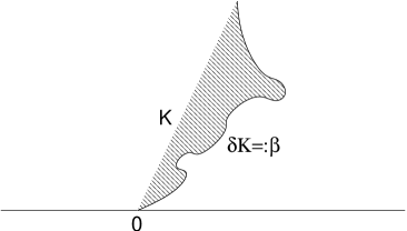
Figure 1: The set $K$ and its right-boundary $\beta$.

Here we will focus mainly on the right boundary of such sets $K$ (which -in the one-sided case- is an equivalent way of describing $K$) that will be denoted by $\beta$. It is shown in [33] that this curve is an SLE$(8/3,\rho)$ for some $\rho=\rho(h)$. In particular, the Hausdorff dimension of all these curves $\beta$ is $4/3$.

The most important examples of such sets $\beta$ are:

• The SLE_8/3 curve itself. In fact, it is the only simple curve satisfying the two-sided restriction property. The corresponding exponent $h$ is $5/8$.

• If one takes the “right-boundary” of a Brownian excursion from 0 to $\infty$ in the upper-half plane (this process is a Markov process that can be loosely described as Brownian motion conditioned never to hit the real line). This corresponds to the exponent $h=1$.

This last example can in fact be generalized to all $h<1$: If one takes the “right-boundary” of a Brownian motion started from the origin that is

• Conditioned never to hit the positive half-axis,

• Reflected off the negative half-axis with a fixed well-chosen angle $\theta(h)$,

then, it satisfies the one-sided restriction property with exponent $h$. See [33] for more details.

Also, it is easy to see that if $\beta_{1},\beta_{2},\ldots,\beta_{N}$ are $N$ such independent curves with respective exponents $h_{1},h_{2},\ldots,h_{N}$, then the right-boundary $\beta$ of $\beta_{1}\cup\ldots\cup\beta_{N}$ also satisfies the one-sided restriction property with exponent $h_{1}+\cdots+h_{N}$. This is simply due to the fact that

$$P[\beta\cap(\mathbb{H}\setminus H)=\emptyset]=\prod_{j=1}^{j=N}P[\beta_{j}\cap(\mathbb{H}\setminus H)=\emptyset]=\Phi_{H}^{\prime}(0)^{h_{1}+\cdots+h_{N}}$$

for all $H\in{\cal H}_{+}$.

In particular, this shows that any one-sided restriction measure can be constructed using the union of independent (conditioned and reflected) Brownian motions.

3 Boundary correlation functions

Suppose now that the random simple curve $\beta$ satisfies the one-sided restriction property. For each real positive $x$ and ${\varepsilon}$, define the event

$$E_{\varepsilon}(x):=\{\beta\cap[x,x+i{\varepsilon}\sqrt{2}]\not=\emptyset\}.$$

The one-sided restriction property of $\beta$ shows that

$$P[E_{{\varepsilon}_{1}}(x_{1})\cup\ldots\cup E_{{\varepsilon}_{n}}(x_{n})]=1-\Phi_{\mathbb{H}\setminus\cup_{j=1}^{n}[x_{j},x_{j}+i{\varepsilon}_{j}\sqrt{2}]}^{\prime}(0)^{h},$$

for all positive $x_{j}$’s and ${\varepsilon}_{j}$’s. These derivatives can (in principle) be determined ($\Phi^{-1}$ is a simple Schwarz-Christoffel transformation, see [1]). This (by a simple inclusion-exclusion formula) yields the values of the probabilities

$$f(x_{1},{\varepsilon}_{1},\ldots,x_{n},{\varepsilon}_{n}):=P[E_{{\varepsilon}_{1}}(x_{1})\cap\ldots\cap E_{{\varepsilon}_{n}}(x_{n})]$$

in terms of $x_{1},\ldots,x_{n},{\varepsilon}_{1},\ldots,{\varepsilon}_{n}$. For example, when $n=1$,

$$f(x,{\varepsilon})=P[E_{\varepsilon}(x)]=1-\left(\frac{x}{\sqrt{x^{2}+2{\varepsilon}^{2}}}\right)^{h}.$$

In particular, $f(x,{\varepsilon})\sim{\varepsilon}^{2}h/x^{2}$ when ${\varepsilon}\to 0$. We then define $B_{1}^{(h)}(x)=h/x^{2}=\lim_{{\varepsilon}\to 0}{\varepsilon}^{-2}f(x,{\varepsilon})$.

More generally, one can define the functions $B_{n}=B_{n}^{(h)}$ as

$$B_{n}(x_{1},\ldots,x_{n}):=\lim_{{\varepsilon}_{1},\ldots,{\varepsilon}_{n}\to 0}{\varepsilon}_{1}^{-2}\ldots{\varepsilon}_{n}^{-2}f(x_{1},{\varepsilon}_{1},\ldots,x_{n},{\varepsilon}_{n}).$$ (1)

Figure 2: The event $E=E_{\varepsilon}(x_{1})\cap E_{\varepsilon}(x_{2})\cap E_{\varepsilon}(x_{3})$.

An indirect way to justify the existence of the existence of the limit in (1) goes as follows: First, note that when $h=1$, the description of $\beta$ as the right-boundary of a Brownian excursion yields the existence of $B_{n}^{(1)}$ and the following explicit expression:

$$B_{n}^{(1)}(x_{1},\ldots,x_{n})=\sum_{s\in\sigma_{n}}\prod_{j=1}^{n-1}(x_{s(j)}-x_{s(j-1)})^{-2},$$

where $\sigma_{n}$ denotes the group of permutations of $\{1,\ldots,n\}$ and by convention $x_{s(0)}=0$. This is due to the fact that $\beta$ intersects all these slits if and only if the Brownian excursion itself intersects all these slits. One then decomposes this event according to the order with which the excursion actually hits them, and one uses its strong Markov property.

Similarly, an analogous reasoning using the Brownian motions reflected on the negative half-axis, and conditioned not to hit the positive half-axis (and its strong Markov property), yields the existence of the limit in (1) for all $h<1$.

Also, since the right-boundary of the union $K_{1}\cup\ldots\cup K_{N}$ of $N$ independent sets satisfying the restriction property with exponents $h_{1},\ldots,h_{N}$ satisfies the one-sided restriction property with exponent $h_{1}+\cdots+h_{N}$, we get easily the existence of the limit in (1) for all $h$ (using the existence when $h_{1},\ldots,h_{N}\leq 1$), and the following property of the functions $B$: For all $R:\{1,\ldots,n\}\to\{1,\ldots,N\}$, write $r(j)=\hbox{card}(R^{-1}\{j\})$. Then,

$$B_{n}^{(h_{1}+\cdots+h_{N})}(x_{1},\ldots,x_{n})=\sum_{R}\prod_{j=1}^{N}B_{r(j)}^{(h_{j})}(x_{R^{-1}\{j\}}),$$ (2)

where $B_{0}=1$ and $x_{I}$ denotes the vector with coordinates $x_{k}$ for $k\in I$. This yields a simple explicit formula for $B^{(n)}$ when $n$ is a positive integer.

In the general case, one way to compute $B_{n}^{(h)}$ is to use the following inductive relation (together with the convention $B^{(h)}_{0}\equiv 1$):

Proposition 1.

For all $n\in\mathbb{N}$, $x,x_{1},\ldots,x_{n}\in\mathbb{R}_{+}$,

$$B_{n+1}^{(h)}(x,x_{1},x_{2},\ldots,x_{n})\ =\ \frac{h}{x^{2}}B_{n}^{(h)}(x_{1},\ldots,x_{n})$$ (3)

$$-\sum_{j=1}^{n}\left\{(\frac{1}{x_{j}-x}+\frac{1}{x})\partial_{x_{j}}-\frac{2}{(x_{j}-x)^{2}}\right\}B_{n}^{(h)}(x_{1},\ldots,x_{n}).$$

This relation plays the role of the Ward identities in the CFT formalism.

Proof. Suppose now that the real numbers $x_{1},\ldots,x_{n}$ are fixed and let us focus on the event $E=E_{\varepsilon}(x_{1})\cap\ldots\cap E_{\varepsilon}(x_{n})$. Let us also choose another point $x\in\mathbb{R}$ and a small $\delta$. Now, either the curve $\beta$ avoids $[x,x+i\delta\sqrt{2}]$ or it does hit it. This additional slit is hit (as well as the $n$ other ones) with a probability $A$ comparable to

$${\varepsilon}^{2n}\delta^{2}B_{n+1}(x_{1},\ldots,x_{n},x)$$

when both $\delta$ and ${\varepsilon}$ vanish. On the other hand, the image of $\beta$ conditioned to avoid $[x,x+i\delta\sqrt{2}]$ under the map

$$\varphi(z)=\Phi_{\mathbb{H}\setminus[x,x+i\delta\sqrt{2}]}=\sqrt{(z-x)^{2}+2\delta^{2}}-\sqrt{x^{2}+2\delta^{2}}$$

has the same law as $\beta$. In particular, we get immediately that

$$A^{\prime} := {\bf P}[E\mid\beta\cap[x,x+i\delta\sqrt{2}]=\emptyset]$$

$$\sim {\varepsilon}^{2n}\prod_{j=1}^{n}|\varphi^{\prime}(x_{j})|^{2}B(\varphi(x_{1}),\ldots,\varphi(x_{n}))$$

when ${\varepsilon}\to 0$ (this square for the derivatives can be interpreted as the fact that the “boundary exponent” for restriction measures is always 2). But when $\delta$ vanishes,

$$\varphi(z)=z+{\delta^{2}}\left(\frac{1}{z-x}+\frac{1}{x}\right)+o(\delta^{2})$$

and

$$\varphi^{\prime}(z)=1-\frac{\delta^{2}}{(z-x)^{2}}+o(\delta^{2}).$$

On the other hand,

$${\bf P}[E]=A+A^{\prime}{\bf P}[\beta\cap[x,x+i\delta\sqrt{2}]=\emptyset]$$ (4)

is independent of $\delta$ and

$${\bf P}[\beta\cap[x,x+i\delta\sqrt{2}]=\emptyset]=\varphi^{\prime}(0)^{h}=1-\frac{h\delta^{2}}{x^{2}}+o(\delta^{2})$$

when $\delta\to 0$. Looking at the $\delta^{2}$ term in the $\delta$-expansion of (4), we get (3). ∎

4 Highest-weight representations

We now define, for all $N\in\mathbb{Z}$, the operators

$${\cal L}_{N}=\sum_{j}\{-x_{j}^{1+N}\partial_{x_{j}}-2(N+1)x_{j}^{N}\}$$

acting on functions of the real variables $x_{1},x_{2},\ldots$. In fact, one should (but we will omit this) make precise the range of $j$ i.e. define ${\cal L}_{N}$ on the union over $n$ of the spaces $V_{n}$ of functions of $n$ variables $x_{1},\ldots,x_{n}$.

Note that these operators satisfy the commutation relation

$$[{\cal L}_{N},{\cal L}_{M}]=(N-M){\cal L}_{N+M}$$

just as the operators $L_{N}$ do. In other words, the vector space generated by these operators is (isomorphic to) the the Witt algebra, i.e. the Lie algebra of vector fields on the unit circle (this is classical, see e.g. [15]).

Note also that one can rewrite the Ward identity in terms of these operators as:

$$B_{n+1}^{(h)}(x,x_{1},\ldots,x_{n})=\frac{h}{x^{2}}B_{n}^{(h)}(x_{1},\ldots,x_{n})+\sum_{N\geq 1}x^{N-2}{\cal L}_{-N}B_{n}^{(h)}(x_{1},\ldots,x_{n}).$$ (5)

We are now going to consider vectors $w=(w_{0},w_{1},w_{2},\ldots)$ such that for each $n$, $w_{n}$ is a function of $n$ variables $x_{1},\ldots,x_{n}$. An example of such a vector is

$$B=B^{(h)}=(B_{0}^{(h)},B_{1}^{(h)},B_{2}^{(h)},\ldots)$$

where $B_{0}^{(h)}$ is set to be equal to $1$. For convenience we will fix $h$ and not always write the $(h)$ superscript.

For such a vector $w$, we define for all $N\in\mathbb{Z}$ the operator $l_{N}$ in such a way that

$$w_{n+1}(x,x_{1},\ldots,x_{n})=\sum_{N\in\mathbb{Z}}x^{N-2}(l_{-N}(w))_{n}(x_{1},\ldots,x_{n}).$$

In other words, the $n$-variable component $(l_{N}(w))_{n}$ of $l_{N}(w)$ is the $x^{-N-2}$ term in the Laurent expansion of $w_{n+1}(x,x_{1},\ldots,x_{n})$ with respect to $x$.

For example, the Ward identity (5) gives the values of $l_{N}(B)$:

$$l_{N}(B)=\left\{\begin{array}[]{l@{\hbox{ if }}l}(0,0,\ldots)&N>0\\ (hB_{0},hB_{1},\ldots)&N=0\\ ({\cal L}_{N}B_{0},{\cal L}_{N}B_{1},\ldots)&N<0\end{array}\right.$$ (6)

We insist on the fact that $l_{N}(B)$ does not coincide with ${\cal L}_{N}(B)$ for non-negative $N$’s. For instance,

$${\cal L}_{0}(B_{1})=0\not=hB_{1}=(l_{0}B)_{1}.$$

But the identity for negative $N$’s can be iterated as follows:

Lemma 1.

For all $k\geq 1$ and negative $N_{1},\ldots,N_{k}$,

$$(l_{N_{1}}\cdots l_{N_{k}}B)_{n}={\cal L}_{N_{1}}\ldots{\cal L}_{N_{k}}B_{n}.$$ (7)

Proof of the Lemma. This is a rather straightforward consequence of (5). We have just seen that it holds for $k=1$. Assume that (7) holds for some given integer $k\geq 1$. Then, for all negative $N_{2},\ldots,N_{k}$,

$$({\cal L}_{N_{2}}\cdots{\cal L}_{N_{k}}B)_{n+1}(x,x_{1},\ldots,x_{n})$$

$$= u+\sum_{N\leq-1}x^{-N-2}{\cal L}_{N}{\cal L}_{N_{2}}\ldots{\cal L}_{N_{k}}B_{n}(x_{1},\ldots,x_{n})$$

where $u$ is a Laurent series in $x$ such that $u(x,x_{1},\ldots,x_{n})=O(x^{-2})$ when $x\to\infty$. We then apply ${\cal L}_{N_{1}}$ (viewed as acting on the space of functions of the $n+1$ variables $x,x_{1},\ldots,x_{n}$) to this equation, where $N_{1}<0$. There are two $x^{-N-2}$ terms in the expansion on the right-hand side: The first one is simply

$$x^{-N-2}{\cal L}_{N_{1}}{\cal L}_{N}{\cal L}_{N_{2}}\ldots{\cal L}_{N_{k}}B_{n}(x_{1},\ldots,x_{n}).$$

The second one comes from the term

$$({\cal L}_{N_{1}}x^{-N-N_{1}-2}){\cal L}_{N+N_{1}}{\cal L}_{N_{2}}\ldots{\cal L}_{N_{k}}B_{n}(x_{1},\ldots,x_{n})$$

$$= (N-N_{1})x^{-N-2}{\cal L}_{N+N_{1}}{\cal L}_{N_{2}}\ldots{\cal L}_{N_{k}}B_{n}(x_{1},\ldots,x_{n}).$$

The sum of these two contributions is indeed

$$x^{-N-2}{\cal L}_{N}{\cal L}_{N_{1}}\ldots{\cal L}_{N_{k}}B_{n}(x_{1},\ldots,x_{n})$$

because of the commutation relation

$${\cal L}_{N_{1}}{\cal L}_{N}+(N-N_{1}){\cal L}_{N+N_{1}}={\cal L}_{N}{\cal L}_{N_{1}}.$$

This proves (7) for $k+1$. ∎

We now define, the vector space $V$ generated by the vector $B$ and all vectors $l_{N_{1}}\ldots l_{N_{k}}B$ for negative $N_{1},\ldots,N_{k}$ and positive $k$ (we will refer to these vectors as the generating vectors of $V$). Then:

Proposition 2.

For all $v\in V$, for all $M,R$ in $\mathbb{Z}$,

$$l_{M}(v)\in V\hbox{ and }[l_{M},l_{R}]v=(M-R)l_{M+R}v.$$

We insist again on the fact that $l_{N}$ only coincides with ${\cal L}_{N}$ for negative $N$. Also, the commutation relation for the $l_{N}$’s does not hold for a general vector. The above statement only says that it is valid on this special vector space $V$.

Proof. Note that the commutation relation holds for negative $R$ and $M$’s because of Lemma 1.

Suppose now that $N_{1},\ldots,N_{k}$ are negative. Then,

$${\cal L}_{N_{1}}\ldots{\cal L}_{N_{k}}B_{n+1} = \sum_{N\leq 0,I}{\cal L}_{N_{i_{1}}}\ldots{\cal L}_{N_{i_{r}}}(x^{-2-N})$$

$$\hskip 28.45274pt\times{\cal L}_{N_{j_{1}}}\ldots{\cal L}_{N_{j_{s}}}(l_{N}B)_{n}(x_{1},\ldots,x_{n})$$

where the sum is over all $I:=\{i_{1},\ldots,i_{r}\}\subset\{1,\ldots,k\}$. One then writes $\{j_{1},\ldots j_{s}\}=\{1,\ldots,k\}\setminus\{i_{1},\ldots,i_{r}\}$ (and the $i$’s and $j$’s are increasing). We use $l_{N}(B)_{n}$ instead of ${\cal L}_{N}B_{n}$ to simplify the expression (otherwise the case $N=0$ would have to be treated separately).

Since

$${\cal L}_{N_{i_{1}}}\ldots{\cal L}_{N_{i_{k}}}(x^{-2-N})$$

$$= (N-2N_{i_{r}})(N-N_{i_{r}}-2N_{i_{r-1}})\ldots$$

$$\ldots(N-N_{i_{r}}-\ldots-N_{i_{2}}-2N_{i_{1}})x^{-2-N+N_{i_{1}}+\cdots+N_{i_{k}}},$$

it follows immediately that for all integer $M$,

$$(l_{M}l_{N_{1}}\ldots l_{N_{k}}B)_{n}$$ (8)

$$= \sum_{I:\ M+N_{i_{1}}+\cdots+N_{i_{r}}\leq 0}(M+N_{i_{1}}+\ldots+N_{i_{r-1}}-N_{i_{r}})\ldots(M-N_{i_{1}})$$

$$\hskip 28.45274pt\times{\cal L}_{N_{j_{1}}}\ldots{\cal L}_{N_{j_{s}}}(l_{M+N_{i_{1}}+\ldots+N_{i_{r}}}B)_{n}$$

This implies that indeed, $l_{M}(V)\subset V$. When $M\leq 0$, then for any $i_{1},\ldots,{i_{r}}$, $M+N_{i_{1}}+\ldots+N_{i_{r}}\leq 0$, so that the sum is over all $I$.

Suppose now that $M\geq 0$, $R<0$, and consider $v=l_{N_{1}}\ldots l_{N_{k}}$ for some fixed negative $N_{1},\ldots,N_{k}$. We can apply (8) to get the expression of $l_{R+M}v$, of $l_{M}l_{R}v$ and of $l_{M}v$. Furthermore, we can use the Lemma to deduce the following expression for $l_{R}l_{M}v$:

$$(l_{R}l_{M}v)_{n}$$

$$= \sum_{I:\ M+N_{i_{1}}+\cdots+N_{i_{r}}\leq 0}(M+N_{i_{1}}+\ldots+N_{i_{r-1}}-N_{i_{r}})\ldots(M-N_{i_{1}})$$

$$\hskip 28.45274pt\times{\cal L}_{R}{\cal L}_{N_{j_{1}}}\ldots{\cal L}_{N_{j_{s}}}(l_{M+N_{i_{1}}+\ldots+N_{i_{r}}}B)_{n}$$

On the other hand,

$$(l_{M}l_{R}v)_{n}$$

$$= \sum_{I_{0}:\ M+N_{i_{0}}+\cdots+N_{i_{r}}\leq 0}(M+N_{i_{0}}+\ldots+N_{i_{r-1}}-N_{i_{r}})\ldots(M-N_{i_{0}})$$

$$\hskip 28.45274pt\times{\cal L}_{N_{j_{1}}}\ldots{\cal L}_{N_{j_{s}}}(l_{M+N_{i_{0}}+\ldots+N_{i_{r}}}B)_{n},$$

where this time, the sum is over $\{i_{0},\ldots,i_{r}\}\subset\{0,\ldots,k\}$, and we put $R=N_{0}$. The difference between these two expressions is due to the terms (in the latter) where $i_{0}=0$:

$$[l_{M},l_{R}]v$$

$$= (M-R)\sum_{I:\ M+N_{i_{1}}+\cdots+N_{i_{r}}\leq 0}(M+R+N_{i_{1}}+\ldots+N_{i_{r-1}}-N_{i_{r}})\ldots$$

$$\ldots(M+R-N_{i_{1}}){\cal L}_{N_{j_{1}}}\ldots{\cal L}_{N_{j_{s}}}(l_{M+R+N_{i_{1}}+\ldots+N_{i_{r}}}B)_{n}$$

$$= (M-R)l_{M+R}.$$

This proves the commutation relation for negative $R$ and arbitrary $M$.

Finally, to prove the commutation relation when both $R$ and $M$ are negative and $v=l_{N_{1}}\ldots l_{N_{k}}$ as before, it suffices to use the previously proved commutation relations to write $l_{M}v$, $l_{R}v$ and $l_{M+R}v$ as linear combination of the generating vectors of $V$. Then, one can iterate this procedure to express $[l_{M},l_{R}]v$ as a linear combination of the generating vectors of $V$. Since this formal algebraic calculation is identical to that one would do in the Lie algebra ${\cal A}$, one gets indeed $[l_{M},l_{R}]v=(M-R)l_{M+R}$, which therefore also holds for any $v\in V$. ∎

To put it differently, to each (one-sided) restriction measure, one can simply associate a highest-weight representation of the Lie algebra ${\cal A}$ (without central extension) acting on a certain space of function-valued vectors. The value of the highest weight is the exponent of the restriction measure.

Note that the right-sided boundary of a simply connected set $K$ satisfying the two-sided restriction property satisfies the one-sided restriction property (so that one can also associate a representation to it). In this case, the function $B_{n}$ also represents the limiting value of

$${\varepsilon}^{-2n}P(K\hbox{ intersects all slits }[x_{j},x_{j}+i{\varepsilon}\sqrt{2}],j=1,\ldots,n)$$

even for negative values of some $x_{j}$’s.

5 Evolution and degeneracy

5.1 SLE_8/3

We are now going to see how to combine the previous considerations with a Markovian property. For instance, does there exist a value of $\kappa$ such that SLE_κ satisfies the restriction property? We know from [33] that the answer is yes, that the value of $\kappa$ is $8/3$ and that the corresponding exponent is $5/8$. This “boundary exponent” for SLE_8/3 has appeared before in the theoretical physics literature (see e.g. [14]) as the boundary exponent for long self-avoiding walks (which is consistent with the conjecture [32] that this SLE is the scaling limit of the half-plane self-avoiding walk). This exponent was identified as the only possible highest-weight of a highest-weight representation of ${\cal A}$ that is degenerate at level two.

We are now going to see that indeed, the Markovian property of SLE is just a way of saying that the two vectors $l_{-2}(B)$ and $l_{-1}^{2}(B)$ are not independent. This shows (without using the computations in [33]) why the values $\kappa=8/3$, $h=5/8$ pop out.

Suppose that $\beta$ is an SLE_κ. Consider the event $E:=E_{{\varepsilon}_{1}}(x_{1})\cap\ldots\cap E_{{\varepsilon}_{n}}(x_{n})$ as in the definition of $B_{n}^{(h)}$. If one considers the conditional probability of $E$ given $\beta$ up to time $t$, then it is the probability that an (independent) SLE $\tilde{\beta}$ hits the (curved) slits $f_{t}([x_{j},x_{j}+i{\varepsilon}_{j}\sqrt{2}])$. At first order, this is equivalent to hitting the straight slits

$$[f_{t}(x_{j}),f_{t}(x_{j})+i{\varepsilon}_{j}\sqrt{2}f_{t}^{\prime}(x_{j})].$$

If the SLE satisfies the restriction property with exponent $h$, then this means that

$$f_{t}^{\prime}(x_{1})^{-2}\ldots f_{t}^{\prime}(x_{n})^{-2}B_{n}^{(h)}(f_{t}(x_{1}),\ldots,f_{t}(x_{n}))$$

is a local martingale. Recall that

$$\partial_{t}f_{t}(x)=-\sqrt{\kappa}db_{t}+\frac{2}{f_{t}(x)}\hbox{ and }\partial_{t}f_{t}^{\prime}(x)=\frac{-2f_{t}^{\prime}(x)}{f_{t}(x)^{2}}.$$

Hence, since the drift term of the previous local martingale vanishes, Itô’s formula yields

$$\frac{\kappa}{2}{\cal L}_{-1}^{2}B_{n}-2{\cal L}_{-2}B_{n}=0$$

for all $n\geq 1$. Note that the operators are ${\cal L}$’s, and not $L$’s as in the crossing probability formulae, because of the local scaling properties of the functions $B$.

In other words, $l_{-2}(B)$ and $l_{-1}^{2}(B)$ are collinear and the previously described highest-weight representation of ${\cal A}$ must be degenerate at level two. It is elementary to deduce the values of $h$ and $\kappa$, using the fact that

$$l_{2}(\frac{\kappa}{2}l_{-1}^{2}-2l_{-2})B=(3\kappa-8)l_{0}B=0$$

which implies that $\kappa=8/3$ and

$$l_{1}(\frac{\kappa}{2}l_{-1}^{2}-2l_{-2})B=\frac{\kappa}{2}(4l_{-1}l_{0}B+2l_{-1}B)-6l_{-1}B=(2\kappa h+\kappa-6)l_{-1}B=0$$

which then implies that $h=5/8$.

5.2 The cloud of bubbles

We are now going to use the description of the “restriction paths” $\beta$ via SLE curves to which one adds a Poissonian cloud of Brownian bubbles, as explained in [33]. Let us briefly recall how it goes. Consider an SLE_κ for $\kappa<8/3$. As we have just seen, it does not satisfy the restriction property. However, if one adds to this curve an appropriate random cloud of Brownian loops, then the obtained set satisfies the two-sided restriction property for a certain exponent $h>5/8$ (and its right-boundary $\beta$ satisfies the one-sided restriction property). More details and properties of the Brownian loop-soup and the procedure of adding loops can be found in [33, 35].

Intuitively this phenomenon can be understood from the case, where $\kappa=2$: SLE₂ is the scaling limit of the loop-erased random walk excursion (see [31]). Adding Brownian loops to it, one should (in principle) recover the Brownian excursion that satisfies the restriction property with parameter $h=1$.

More generally, let $\kappa<8/3$ be fixed, and consider an SLE_κ curve $\gamma$, with its usual time-parametrization. There exists a natural (infinite) measure on Brownian bubbles in $\mathbb{H}$ rooted at the origin. This is a measure supported on Brownian paths of finite length in $\mathbb{H}$ that start and end at the origin (more generally, we say that a bubble in $H$ rooted at $x\in\partial H$ is a path $\eta$ of finite length $T$ such that $\eta(0,T)\in H$ and $\eta(0)=\eta(T)=x$). Consider a Poisson point process of these Brownian bubbles in $\mathbb{H}$, with intensity $\lambda$ (more precisely, $\lambda$ times the measure on Brownian bubbles). A realization of this point process is a family $(\hat{\eta}_{t},t\geq 0)$ such that for all but a random countable set $\{t_{j}\}$ of times, $\hat{\eta}_{t}=\emptyset$ and for the times $t_{j}$, $\hat{\eta}_{t_{j}}$ is a (Brownian) bubble in $\mathbb{H}$ rooted at the origin. We then define for all $t$, $\eta_{t}=f_{t}^{-1}(\hat{\eta}_{t})$, so that $\eta_{t}$ is empty if $t\notin\{t_{j}\}$ and is a bubble in $\mathbb{H}\setminus\gamma[0,t_{j}]$ rooted at $\gamma(t_{j})$ if $t=t_{j}$. Another equivalent way to define this random family $(\eta_{t},t\geq 0)$ via a certain Brownian loop-soup is described in [35].

Define the union $\Gamma$ of $\gamma$ and the bubbles $\eta_{t}$, i.e.

$$\Gamma=\cup_{t\geq 0}(\{\gamma_{t}\}\cup\eta_{t}).$$

We let ${\cal F}_{t}$ denote the $\sigma$-field generated by $(\gamma_{s},\eta_{s},s\leq t)$.

The right outer-boundary $\beta$ (see [33, 35]) of $\Gamma$ then satisfies the restriction property (actually $\Gamma$ satisfies the two-sided restriction property). This is proved in [33] studying the conditional probabilities that $\Gamma$ avoids a given set $A$ with respect to the filtration generated by $\gamma$ alone. As observed in [33], the relation between the density $\lambda(\kappa)$ of the loops that one has to add to the SLE_κ and the exponent $h(\kappa)$ of the corresponding restriction measure (i.e. $h=(6-\kappa)/2\kappa$ and $\lambda=(8-3\kappa)h$) recalls the relation between the central charge and the highest-weight of degenerate highest-weight representations of the Virasoro algebra (which is the central extension of ${\cal A}$). We shall try in this subsection to give one way to explain the relation to representations, via the functions $B_{n}^{(h)}$, and therefore recover these values of $h$ and $\lambda$, just assuming that if one adds the cloud of bubbles with intensity some $\lambda$, one obtains a restriction measure.

It is worthwhile emphasizing that in this context, the functions $B_{n}^{(h)}$ are only indirectly related to the SLE curve via this Poissonian cloud of loops. They do for instance not represent the probabilities that the SLE itself does visit the infinitesimal slits, but the probability that some loops that have been attached to this SLE curve do visits the infinitesimal slits.

Recall that the functions $B_{n}^{(h)}$ are related to a highest-weight representation of ${\cal A}$, as discussed in the previous section. As in the $\kappa=8/3$ case, we will try to obtain an additional information on this representation, using the evolution of the SLE curve. More precisely: How does the (conditional) probability with respect to ${\cal F}_{t}$ of the event $E$ that $\beta$ intersects the $n$ slits $[x_{j},x_{j}+i{\varepsilon}_{j}\sqrt{2}]$ for infinitesimal ${\varepsilon}_{j}$’s evolve with time? Here is a heuristic discussion, that can easily be made rigorous:

Consider an infinitesimal time $\Delta$. Let $\tilde{\Gamma}_{\Delta}$ denote the union of $\gamma[\Delta,\infty)$ and the loops that it does intersect. More precisely,

$$\tilde{\Gamma}_{\Delta}=\cup_{t>\Delta}(\{\gamma_{t}\}\cup\eta_{t}).$$

Typically (for very small $\Delta$), there is no bubble $\eta_{t}$ for $t\in[0,\Delta]$ that does intersect one of these $n$ slits. In this case, the conditional probability of the event $E$ given ${\cal F}_{\Delta}$ is simply the probability that $\tilde{\Gamma}_{\Delta}$ does intersect these $n$ slits (given ${\cal F}_{\Delta}$). The definition of $\gamma$ and of the bubbles show that the conditional law of $f_{\Delta}(\tilde{\Gamma}_{\Delta})$ given ${\cal F}_{\Delta}$ is independent of $\Delta$ (in particular, it is the same as for $\Delta=0$ i.e. the law of $\Gamma$). This shows that (exactly as in the $\kappa=8/3$ case), the conditional probability of $E$ has a drift term due to the distortion of space induced by the SLE (i.e. by $f_{\Delta}$) of the type

$$(\frac{\kappa}{2}{\cal L}_{-1}^{2}B_{n}-2{\cal L}_{-2}B_{n})\Delta.$$

But there is an additional term due to the fact that one might in the small time-interval $[0,\Delta]$, have added a Brownian loop $\eta_{t}$ to the curve that precisely goes through one or several of the $n$ slits $[x_{j},x_{j}+i{\varepsilon}_{j}\sqrt{2}]$. The probability that one has added a loop that goes through the $j$-th slit is of order ${\lambda{\varepsilon}_{j}^{2}}\Delta/{x_{j}^{4}}$. This fact is due to scale-invariance. Here $\lambda$ is the (constant) density of loops that is added on top of the SLE curve (we use this definition for this density $\lambda$ in this paper, as in [33]; in other contexts, replacing $\lambda$ by $\lambda/6$ can be more natural). One way to understand the ${\varepsilon}_{j}^{2}/x_{j}^{4}$ term is that the Brownian bubble has to go from $0$ to the slit, which contributes a factor ${\varepsilon}_{j}^{2}/x_{j}^{2}$, and then back to the origin, which contributes also $1/x_{j}^{2}$. If such a loop has been added, the conditional probability of $E$ is (at first order) the probability that the SLE+loops hits the remaining $n-1$ slits, i.e. $f_{n-1}(x_{\{1,\ldots n\}\setminus\{j\}})\prod_{l\not=j}{\varepsilon}_{l}^{2}$ (here and in the sequel $x_{J}$ stands for $(x_{j_{1}},\ldots,x_{j_{p}})$ when $J=\{j_{1},\ldots,j_{p}\}$). More generally, define $T_{0}=0$, $T_{1}(x)=1/x^{4}$, and for $p\geq 2$,

$$T_{p}(x_{1},\ldots,x_{p})=\sum_{s\in\sigma_{p}}\frac{1}{x_{s(1)}^{2}(x_{s(2)}-x_{s(1)})^{2}\ldots(x_{s(p)}-x_{s(p-1)})^{2}x_{s(p)}^{2}}.$$

Each $s$ corresponds intuitively to an order of visits of the infinitesimal slits by the loop. For $J=\{j_{1},\ldots,j_{p}\}\subset\{1,\ldots,n\}$ with $|J|=p\geq 1$, the probability to add a loop that goes precisely through the slits near $x_{j}$ for $j\in J$ is of the order of

$${\varepsilon}_{j_{1}}^{2}\ldots{\varepsilon}_{j_{p}}^{2}T_{p}(x_{J})\lambda\Delta.$$

We are therefore naturally led to define the operator $U$ by

$$(Uf)_{n}(x_{1},\ldots,x_{n})=\sum_{J\subset\{1,\ldots,n\}}T_{p}(x_{J})\times f_{n-p}(x_{\{1,\ldots n\}\setminus J}).$$

Then, the fact that $P(E|{\cal F}_{t})$ is a martingale, shows that the drift term vanishes i.e. that

$$\left\{\frac{\kappa}{2}{l}_{-1}^{2}-2{l}_{-2}+\lambda U\right\}B=0.$$ (9)

Note that the definitions of $l_{N}$ and $U$ show easily that for any $w=(w_{0},w_{1},\ldots)$ (not only in $V$),

$$([l_{N},U]w)_{n}(x_{1},\ldots,x_{n})=\sum_{J\subset\{1,\ldots,n\}}(l_{N}(T))_{p}(x_{J})\times w_{n-p}(x_{\{1,\ldots n\}\setminus J}).$$

In order to compute $l_{N}(T)_{p}$, one has to look at the Laurent expansion (when $x\to 0$) of $T_{p+1}(x,x_{1},\ldots,x_{p})$. Recall that $T_{1}(x)=1/x^{4}$ and note that for $p\geq 1$,

$$T_{p+1}(x,x_{1},\ldots,x_{p})=2x^{-2}T_{p}(x_{1},\ldots,x_{p})+o(x^{-2})$$ (10)

(the only terms in the sum that contribute to the leading term are those corresponding to $x$ being visited first or last by the loop). It follows that $l_{N}T=0$ if $N>2$ and if $N=1$ (there are no $x^{-N-2}$ terms in the expansion). Also, $l_{2}T=(1,0,0,\ldots)$ (the only case where there is an $x^{-4}$ term is $p+1=1$). Finally, $l_{0}T=2T$ because of (10). Hence,

$$[l_{N},U]=\left\{\begin{array}[]{l@{\hbox{ if }}l}0&N>2\\ \hbox{Id}&N=2\\ 0&N=1\\ 2U&N=0\end{array}\right.$$

This enables as before to relate $\lambda$ to $\kappa$ and $h$:

$$l_{2}(\kappa l_{-1}^{2}/2-2l_{-2})B=l_{2}(-\lambda UB)=-\lambda B-\lambda Ul_{2}B=-\lambda B$$

and

$$l_{1}(\kappa l_{-1}^{2}/2-2l_{-2})B=l_{1}(-\lambda UB)=-\lambda Ul_{1}B=0.$$

This last relation implies that

$$h=\frac{6-\kappa}{2\kappa}$$

and the first one then shows that

$$\lambda=(8-3\kappa)h=\frac{(8-3\kappa)(6-\kappa)}{2\kappa},$$

which are the formulae appearing in [33].

This relation between $h$ and $-\lambda$ is indeed that between the highest-weight and the central charge for a representation of the Virasoro algebra that is degenerate at level two. Recall that if $\tilde{l}_{n}$’s are the generators of the Virasoro Algebra and $C$ its central element, then $[\tilde{l}_{2},\tilde{l}_{-2}]=4\tilde{l}_{0}+C/2$, so the little two by two linear system leading to the determination of $\kappa$ and $h$ for a degenerate highest-weight representation of the Virasoro algebra is the same (and therefore leads to the same expression); roughly speaking, $l_{-2}-\lambda U/2$ plays the role of $\tilde{l}_{-2}$.

Note that the previous considerations involving the Brownian bubbles is valid only in the range $\kappa\in(0,8/3]$ and therefore for $c\leq 0$. This corresponds to the fact that two-sided restriction measures exist only for $h\geq 5/8$. In this case all functions $B^{(h)}_{n}$ are positive for all (real) values of $x_{1},\ldots,x_{n}$.

5.3 Analytic continuation

In the representations that we have just been looking at, we considered simple operators acting on simple rational functions. All the results depend analytically on $\kappa$ (or $h$). In other words, for all real $\kappa$ (even negative!), if one defines the functions $B_{n}^{(h)}$ recursively, the operators $l_{n}$, the vector $B^{(h)}$ and the vector space $V=V^{(h)}$ as before, then one obtains a highest-weight representation of ${\cal A}$ with highest weight $h$. The values of $\kappa$, $\lambda$ and $h$ are still related by the same formula, but do not correspond necessarily to a quantity that is directly relevant to the SLE curve or the restriction measures.

When $h\in(0,5/8)$, the functions $B^{(h)}_{n}$ can still be interpreted as renormalized probabilities for one-sided restriction measures. They are therefore positive for all positive $x_{1},\ldots,x_{n}$ but they can become negative for some negative values of the arguments. The “SLE + bubbles” interpretation of the degeneracy (i.e. of the relation (9)) is no longer valid since the “density of bubbles” becomes negative (i.e. the corresponding central charge is positive). In this case, the local martingales measuring the effect of boundary perturbations are no longer bounded (and do not correspond to conditional probabilities anymore).

For negative $h$, the functions $B_{n}^{(h)}$ can still be defined. This time, the functions $B_{n}^{(h)}$ are not (all) positive, even when restricted on $(0,\infty)^{n}$ and they do not correspond to any restriction measure. These facts correspond to “negative probabilities” that are often implicit in the physics literature.

Note that $c$ (i.e. $-\lambda$) cannot take any value: For positive $\kappa$, $c$ varies in $(-\infty,1)$ and for negative $\kappa$, it varies in $[25,\infty)$. The transformation $\kappa\leftrightarrow-\kappa$ corresponds to the well-know $c\leftrightarrow 26-c$ duality (e.g. [36]).

In other words, the $B_{n}^{(h)}$’s provide the highest-weight representations of ${\cal A}$ with highest weight $h$. Each one is related to a highest-weight representation of the Virasoro algebra that is degenerate at level 2. Furthermore, all $B_{n}^{(h)}$’s are related by (2).

6 Remarks

In order to clarify the state of the art seen from a mathematical perspective, let us now try to sum up things:

• The interfaces of two-dimensional critical models (such as random cluster interfaces, that are very closely related to Potts models) are believed to be conformally invariant in the scaling limit. In some cases, this is proved (critical percolation, uniform spanning trees). In some other cases (Ising, double-domino tiling), some partial results hold. Anyway, to derive conformal invariance, it seems that one has to work on each specific model separately.

• These interfaces can be constructed in a dynamic way i.e. they have a Markovian type property (at least the critical random cluster interfaces, that have the same correlation functions as the Potts models). Therefore, if conformal invariance holds, their scaling limit must be one of the SLE curves. In general, these limits correspond to the SLE curves with $\kappa>4$ that are not simple curves. The correlation functions of the 2D statistical physics model are related to the fractal properties of the SLE curve, but the knowledge of the SLE curve is a much richer information than just the value of the exponents.

• One can understand the dependence of the law of an SLE in a domain with respect to this domain via the restriction properties. This shows that some specific “finite-dimensional observables” of the SLE curves satisfy some relations. This can be reformulated in terms of highest-weight representations of the Lie algebra ${\cal A}$, and explains the relation between the physics models and these representations. Also, it makes it possible to define conformal fields via SLE. However, and we think that this has to be again stressed, since the initial purpose was to understand the statistical physics models and their behaviour, the SLE itself is a more natural way. Also, one should also again emphasize that in the present paper, the “correlation functions” $B_{n}^{(h)}$ do correspond only indirectly with the curve $\gamma$ (via the cloud of Brownian bubbles) when the central charge does not vanish.

All functions described in the present paper deal with the boundary (or “surface”) behaviour of the systems. One may want to develop a similar theory for points lying in the inside of the upper half-plane (“in the bulk”). Beffara’s results [5] (for instance in the case $\kappa=8/3$) provide a first step in this direction, and show that the definition of these correlation functions themselves is not an easy task.

Acknowledgements. Thanks are of course due to Greg Lawler and Oded Schramm, in particular because of the instrumental role played by the ideas developed in the paper [33]. We have also benefited from very useful discussions with Vincent Beffara and Yves Le Jan. R.F. acknowledges support and hospitality of IHES.

——————

Laboratoire de Mathématiques

Université Paris-Sud

91405 Orsay cedex, France

emails: rolandf@ihes.fr, wendelin.werner@math.u-psud.fr

References

- [1] L.V. Ahlfors, Complex Analysis, 3rd Ed., McGraw-Hill, New-York, 1978.
- [2] M. Aizenman (1996), The geometry of critical percolation and conformal invariance, StatPhys 19 (Xiamen 1995), 104-120.
- [3] M. Bauer, D. Bernard (2002), SLEκ growth and conformal field theories, Phys. Lett. B 543, 135-138.
- [4] M. Bauer, D. Bernard (2002), Conformal Field Theories of Stochastic Loewner Evolutions, arxiv:hep-th/0210015, preprint.
- [5] V. Beffara (2002), The dimension of the SLE curves, arxiv:math.PR/0211322, preprint.
- [6] A.A. Belavin, A.M. Polyakov, A.B. Zamolodchikov (1984), Infinite conformal symmetry of critical fluctuations in two dimensions, J. Statist. Phys. 34, 763-774.
- [7] A.A. Belavin, A.M. Polyakov, A.B. Zamolodchikov (1984), Infinite conformal symmetry in two-dimensional quantum field theory. Nuclear Phys. B 241, 333–380.
- [8] J.L. Cardy (1984), Conformal invariance and surface critical behavior, Nucl. Phys. B 240 (FS12), 514–532.
- [9] J.L. Cardy (1992), Critical percolation in finite geometries, J. Phys. A 25, L201-206.
- [10] J.L. Cardy (2002), Conformal Invariance in Percolation, Self-Avoiding Walks and Related Problems, cond-mat/0209638, preprint.
- [11] J. Dubédat (2003), SLE and triangles, Electr. Comm. Probab. 8, 28-42.
- [12] J. Dubédat (2003), SLE() martingales and duality, arxiv:math.PR/0303128, preprint.
- [13] B. Duplantier (2000), Conformally invariant fractals and potential theory, Phys. Rev. Lett. 84, 1363-1367.
- [14] B. Duplantier, H. Saleur (1986), Exact surface and wedge exponents for polymers in two dimensions, Phys. Rev. Lett. 57, 3179-3182.
- [15] B.L. Feigin, D.B. Fuks (1982), Skew-symmetric invariant differential operators on the line and Verma modules over the Virasoro algebra, Functional Anal. Appl. 16, 114–126.
- [16] E. Frenkel, D. Ben-Zvi, Vetrex Algebras and Algebraic curves, A.M.S. monographs 88, 2001.
- [17] R. Friedrich, J. Kalkkinen (2003), in preparation.
- [18] R. Friedrich, W. Werner (2002), Conformal fields, restriction properties, degenerate representations and SLE, C.R. Acad. Sci. Paris Ser. I. Math. 335, 947-952.
- [19] P. Goddard, D. Olive (Ed.), Kac-Moody and Virasoro algebras. A reprint volume for physicists. Advanced Series in Mathematical Physics 3, World Scientific, 1988.
- [20] C. Itzykson, J.-M. Drouffe, Statistical field theory. Vol. 2. Strong coupling, Monte Carlo methods, conformal field theory, and random systems, Cambridge University Press, Cambridge, 1989.
- [21] C. Itzykson, H. Saleur, J.-B. Zuber (Ed), Conformal invariance and applications to statistical mechanics, World Scientific, 1988.
- [22] V.G. Kac, Infinite-dimensional Lie Algebras, 3rd Ed, CUP, 1990.
- [23] V.G. Kac, A.K. Raina, Bombay lectures on highest weight representations of infinite-dimensional Lie algebras. Advanced Series in Mathematical Physics 2, World Scientific, 1987.
- [24] T.G. Kennedy (2002), Monte-Carlo tests of Stochastic Loewner Evolution predictions for the 2D self-avoiding walk, Phys. Rev. Lett. 88, 130601.
- [25] R. Langlands, Y. Pouliot, Y. Saint-Aubin (1994), Conformal invariance in two-dimensional percolation, Bull. A.M.S. 30, 1–61.
- [26] G.F. Lawler (2001), An introduction to the stochastic Loewner evolution, Proceeding of a conference on random walks, ESI Vienne, to appear.
- [27] G.F. Lawler, O. Schramm, W. Werner (2001), Values of Brownian intersection exponents I: Half-plane exponents, Acta Mathematica 187, 237-273.
- [28] G.F. Lawler, O. Schramm, W. Werner (2001), Values of Brownian intersection exponents II: Plane exponents, Acta Mathematica 187, 275-308.
- [29] G.F. Lawler, O. Schramm, W. Werner (2002), Values of Brownian intersection exponents III: Two sided exponents, Ann. Inst. Henri Poincaré 38, 109-123.
- [30] G.F. Lawler, O. Schramm, W. Werner (2002), One-arm exponent for critical 2D percolation, Electronic J. Probab. 7, paper no.2.
- [31] G.F. Lawler, O. Schramm, W. Werner (2001), Conformal invariance of planar loop-erased random walks and uniform spanning trees, arXiv:math.PR/0112234, Ann. Prob., to appear.
- [32] G.F. Lawler, O. Schramm, W. Werner (2002), On the scaling limit of planar self-avoiding walks, arXiv:math.PR/0204277, in Fractal geometry and application, A jubilee of Benoit Mandelbrot, AMS Proc. Symp. Pure Math., to appear.
- [33] G.F. Lawler, O. Schramm, W. Werner (2002), Conformal restriction. The chordal case, arXiv:math.PR/0209343, J. Amer. Math. Soc., to appear.
- [34] G.F. Lawler, W. Werner (2000), Universality for conformally invariant intersection exponents, J. Europ. Math. Soc. 2, 291-328.
- [35] G.F. Lawler, W. Werner (2003), The Brownian loop-soup, arXiv:math.PR/0304419, preprint.
- [36] Yu. A. Neretin (1994), Representations of Virasoro and affine Lie Algebras, in Representation theory and non-commutative harmonic analysis I (A.A. Kirillov Ed.), Springer, 157-225.
- [37] B. Nienhuis (1984), Coulomb gas description of 2D critical behaviour, J. Stat. Phys. 34, 731-761.
- [38] A.M. Polyakov (1974), A non-Hamiltonian approach to conformal field theory, Sov. Phys. JETP 39, 10-18.
- [39] S. Rohde, O. Schramm (2001), Basic properties of SLE, arXiv:math.PR/0106036, preprint.
- [40] O. Schramm (2000), Scaling limits of loop-erased random walks and uniform spanning trees, Israel J. Math. 118, 221–288.
- [41] O. Schramm (2001), A percolation formula, Electr. Comm. Prob. 6, 115-120.
- [42] S. Smirnov (2001), Critical percolation in the plane: Conformal invariance, Cardy’s formula, scaling limits, C. R. Acad. Sci. Paris S r. I Math. 333 no. 3, 239–244.
- [43] S. Smirnov, W. Werner (2001), Critical exponents for two-dimensional percolation, Math. Res. Lett. 8, 729-744.
- [44] W. Werner (2002), Random planar curves and Schramm-Loewner Evolutions, Lecture Notes of the 2002 St-Flour summer school, Springer, to appear.
——————