Last Branching in Directed Last Passage Percolation

Abstract

The $1+1$ dimensional directed polymers in a Poissonean random environment is studied. For two polymers of maximal length with the same origin and distinct end points we establish that the point of last branching is governed by the exponent for the transversal fluctuations of a single polymer. We also investigate the density of branches.

Keywords: First passage percolation
AMS Subject Classification: Primary $60K35$, Secondary $82B44$
Running Title: Last Branching

1 Introduction and main result

First passage percolation was invented as a simple model for the spreading of a fluid in a porous medium. One imagines that the fluid is injected at the origin. Upon spreading the time it takes to wet across a given bond is postulated to be random. In the directed version the wetting is allowed along a preferred direction only. The task is then to study the random shape of the wetted region at some large time $t$. The existence of a deterministic shape as $t\to\infty$ follows from the subadditive ergodic theorem [Ke]. The shape fluctuations are more difficult to analyse and only some bounds are available [Pi].

A spectacular progress has been achieved recently by Baik, Deift, and Johansson [BDJ], who prove that for directed first passage percolation in two dimensions the wetting time measured along a fixed ray from the origin has fluctuations of order $t^{1/3}$. The amplitude has a non-Gaussian distribution. In fact it is Tracy-Widom distributed [TW], a distribution known previously from the theory of Gaussian random matrices. Of course, such a detailed result is available only for a very specific model. In this model the wetting time is negative, which can be converted into a positive one at the expense of studying last rather than first passage percolation, hence our title. One thereby loses the physical interpretation of the spreading of a fluid. But directed first and last passage percolation models are expected to be in the same universality class under the condition that along the ray under consideration the macroscopic shape has a non-zero curvature [KMH, PS].

Such detailed results are available only for a few last passage percolation models, among them the Poissonean model studied in [BDJ]. It was first introduced by Hammersley [Ha], cf. also the survey by Aldous and Diaconis [AD]. We start from a Poisson point process on $\mathbb{R}_{+}^{2}$ with intensity one. Let $(x,y)\prec(x^{\prime},y^{\prime})$ if $x<x^{\prime}$ and $y<y^{\prime}$. For a given configuration $\omega$ of the Poisson process and two points $S\prec E\in\mathbb{R}_{+}^{2}$ a directed polymer starting at $S$ and ending at $E$ is a piecewise linear path $\pi$ obtained by connecting $S$ and $E$ through a subset $\{q_{1},\ldots,q_{N}\}$ of points in $\omega$ such that $S\prec q_{1}\prec\cdots\prec q_{N}\prec E$. The length, $l(\pi)$, of the directed polymer $\pi$ is the number of Poisson points visited by $\pi$. We denote by $\Pi(S,E,\omega)$ the set of all directed polymers from $S$ to $E$ for given $\omega$ and we are interested in directed polymers which have maximal length. In general there will be several of these and we denote by $\Pi_{\max}(S,E,\omega)$ the set of maximizers, i.e. of directed polymers in $\Pi(S,E,\omega)$ with maximal length

$$L(S,E)(\omega)=\max_{\pi\in\Pi(S,E,\omega)}l(\pi).$$

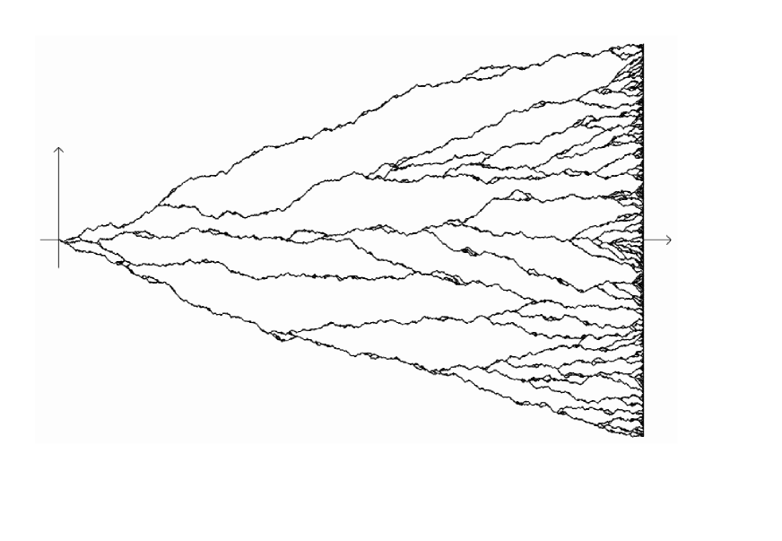
Figure 1: Set of all maximizers from the origin to the line $U_{t}$. The sample uses $\sim 8\cdot 10^{6}$ Poisson points, which in our units correspond to $t=2000$. Only the section $[0,1]\times[-1/6,1/6]$ is shown.

For the specific choice $S=(0,0)$, $E=(t,t)$ let us set $L(S,E)=L(t)$. The distribution function for $L(t)$ can be written in determinantal form as

$$\mathbb{P}(L(t)<a)=\operatorname*{Det}(\mathbbm{1}-P_{a}B_{t})$$ (1)

Here $P_{a}$ and $B_{t}$ are projection operators in $\ell_{2}(\mathbb{Z})$. $P_{a}$ projects onto $[a,\infty)$ and $B_{t}$ is the spectral projection corresponding to the interval $(-\infty,0]$ of the operator $H_{t}$ defined through

$$H_{t}\,\psi(n)=-\psi(n+1)-\psi(n-1)+\frac{n}{t}\psi(n),$$ (2)

i.e. $B_{t}$ is the discrete Bessel kernel. (1) should be compared with the determinantal formula for the largest eigenvalue, $E_{\max}$, of a $N\times N$ Gaussian, $\beta=2$ random matrix, which has the distribution function

$$\mathbb{P}(E_{\max}\leq a)=\operatorname*{Det}(\mathbbm{1}-P_{a}K_{N}).$$ (3)

Here $P_{a}$ and $K_{N}$ are projections in $L^{2}(\mathbb{R})$. $P_{a}$ projects onto the semiinfinite interval $[a,\infty)$ and $K_{N}$ is the spectral projection onto the interval $[0,N]$ of the operator $-\frac{1}{2}\frac{\operatorname*{d}^{2}}{\operatorname*{d}\!x^{2}}+\frac{1}{2}x^{2}$. In the limit of large $t$, under suitable rescaling [PS, TW], both determinantal formulae converge to

$$\operatorname*{Det}(\mathbbm{1}-P_{a}K)$$ (4)

where $K$ is the Airy kernel, i.e. the spectral projection corresponding to $(-\infty,0]$ of the Airy operator $-\frac{\operatorname*{d}^{2}}{\operatorname*{d}\!x^{2}}+x$. (4) is the distribution function for a standard Tracy-Widom random variable $\zeta_{2}$ [TW]. The famous result in [BDJ] states that

$$L(t)\cong 2t+t^{1/3}\zeta_{2}$$ (5)

in the limit of large $t$. In brackets, we remark that the proof in [BDJ] proceeds via Toeplitz and not, as indicated here, via Fredholm determinants.

While (5) gives very precise information about the typical length of directed polymer, it leaves untouched the issue of typical spatial excursions of a maximizing directed polymer. As shown in [Jo], they are in fact of size $t^{2/3}$ away from the diagonal. No information on the distribution is available. The transverse exponent $2/3$ appears also in a somewhat different quantity [PS]. Set $S=(0,0)$, $E=(t-yt^{\nu},t+yt^{\nu})$ and consider the joint distribution of $t^{-1/3}(L(t)-2t)$ and $t^{-1/3}(L(S,E)-2t)$. If $\nu>2/3$, the two random variables become independent as $t\to\infty$ and if $\nu<2/3$ the joint distribution is concentrated on the diagonal. Only for $\nu=2/3$ there is a non-degenerate joint distribution which can be written in terms of suitable determinants involving the Airy operator $-\frac{d^{2}}{dx^{2}}+x$ on $L^{2}(\mathbb{R})$.

In our present work we plan to study a related, but more geometrical quantity, see Figure 1 which displays the directed polymers rotated by $\pi/4$ for better visibility. The root point is always $S=(0,0)$ and the end points lie on the line $U_{t}=\{(t-x,t+x),|x|\leq t\}$. For fixed realization $\omega$ and for each end point $E$ we draw the set of all maximizers. Note that, e.g. for $E=(t,t)$, the directed polymer splits and merges again, which reflects that $\Pi_{\max}(S,E,\omega)$ contains many paths, their number presumably growing exponentially in $t$. The resulting network of lines has some resemblance to a river network with $(0,0)$ as the mouth or to a system of blood vessels, see [Me] for related models. To characterize the network a natural geometrical object is the last branching for a pair of directed polymers with distinct end points [FH]. As in Figure 1 the starting point is always $S=(0,0)$ and the end point $E$ must lie on the line $U_{t}$. If $\pi_{i}$ is a maximizer with start point $S=(0,0)$ and end point $E_{i}\in U_{t}$, $i=1,2$, then the last point in which $\pi_{1}$ and $\pi_{2}$ intersect is denoted by $I(\pi_{1},\pi_{2})$. We define the last intersection point for two sets of maximizers by

$$J(E_{1},E_{2})=I(\pi_{1},\pi_{2})\textrm{ which minimizes }d(I(\pi_{1},\pi_{2}),U_{t})$$

where $d(X,U_{t})$ is the Euclidean distance between $X$ and $U_{t}$. $J(E_{1},E_{2})$ depends on the configuration $\omega$ of the Poisson points but is independent from the choice of the maximizers. $J(E_{1},E_{2})$ is unique since the existence of two distinct last intersection points is in contradiction with the condition of being the last intersection. In particular if $(E_{1})_{1}<(E_{2})_{1}$, then $J(E_{1},E_{2})$ can be obtained by taking the highest maximizer from $0$ to $E_{2}$ and the lowest maximizer from $0$ to $E_{1}$.

Instead of the geometrical intersection, one could require the last intersection point to be a Poisson point. The two maximisers have then necessarily a common root. For the coarse quantities studied here there is no distinction and our results are identical in both cases.

One would expect that the branching is governed again by the transverse exponent $2/3$. More precisely let us assume that

$$d(E_{1},E_{2})=\mathcal{O}(t^{\nu}),\,0\leq\nu<1\textrm{ and }E_{1},E_{2}\in U_{t}.$$

If $\nu=2/3$, the last branching point should have a distance of order $t$ from $U_{t}$ with some on that scale non-degenerate distribution. On the other hand if $\nu>2/3$ the branching will be close to the root and if $\nu<2/3$ the branching will be close to $U_{t}$. Our main result is to indeed single out $\nu=2/3$ and provide some estimates on the tails.

Theorem 1.

Let $E_{1}=(t,t)$ and $E_{2}=E_{1}+yt^{\nu}(-1,1)$ with $y\sim\mathcal{O}(1)$.

• For $\nu>2/3$, there exists a $C(y)<\infty$ such that for all $\sigma>5/3-\nu$,

  $$\lim_{t\to\infty}\mathbb{P}(\{d(0,J(E_{1},E_{2}))\leq C(y)t^{\sigma}\})=1.$$

• For $\nu\leq 2/3$ and for all $\mu<2\nu-1/3$ one has

  $$\lim_{t\to\infty}\mathbb{P}(\{d(J(E_{1},E_{2}),U_{t})\leq t^{\mu}\})=0.$$

In particular for $\nu=2/3$, one can choose $\mu<1$.

Our result does not rule out the possibility that for $\nu=2/3$ the distribution of the last intersection point is degenerate near the origin. In fact the proof exploits geometric aspects for branching points close to $U_{t}$, which cannot be used to obtain sharp results close to the origin.

Another way to characterize the network of Figure 1 is to consider the line density at the cross-section $U_{s}$, equivalently the typical distance between maximizers when crossing $U_{s}$. To have a definition, for given $\omega$ let $\overline{M}_{t}$ be all the maximizers with end points in $U_{t}$ considered as a subset of $\{(x_{1},x_{2}),0\leq x_{1}+x_{2}\leq 2t\}$. $\overline{M}_{t}$ consists of straight segments connecting two points of $\omega$ and straight segments connecting $0$ with a point in $\omega$. In addition there is a union of triangles with base contained in $U_{t}$ and the apex a point of $\omega$. We define $M_{t}$ to be $\overline{M}_{t}$ such that in every triangle only the two sides emerging from the apex are retained. Let

$$N_{t}(s)=\#\textrm{ of points of }M_{t}\cap U_{s},\,0\leq s\leq t.$$ (6)

If $s=c\,t$, $0<c<1$, then the typical distance between lines is of order $t^{2/3}$ and thus one expects

$$N_{t}(ct)\simeq t^{1/3}.$$

On the other hand for a cross-section closer to $U_{t}$ the number of points should increase faster. In particular $N_{t}(t)\simeq t$. This suggests that

$$N_{t}(t-t^{\mu})\simeq t^{g(\mu)}$$

with $g(0)=1$ and $g(1)=1/3$. In the last section we prove the lower bound

$$g(\mu)\geq\frac{5}{6}-\frac{\mu}{2}.$$

2 Last branching

We plan to prove Theorem 1. Before we introduce some notation and state some results of [BDJ] concerning large deviations for the length of maximizers.

For any $w\prec w^{\prime}\in\mathbb{R}_{+}^{2}$, we denote by $[w,w^{\prime}]$ the rectangle with corners at $w$ and $w^{\prime}$ and by $a(w,w^{\prime})$ its area. The maximal length $L(w,w^{\prime})$ is a random variable whose distribution function depends only on $a(w,w^{\prime})$ with $L(w,w^{\prime})\sim 2\sqrt{a(w,w^{\prime})}$. Large deviation estimates for $\mathbb{P}(L(w,w^{\prime})\leq 2\sqrt{a(w,w^{\prime})}+n)$ are proved in [BDJ], Lemma 7.1. We consider the case of $a(w,w^{\prime})\gg 1$ and $|n|\gg 1$. Let

$$\tau=n(\sqrt{a(w,w^{\prime})}+n/2)^{-1/3}.$$

Then there are some positive constants $\theta,T_{0},c_{1},c_{2}$ so that
1. Upper tail: if $T_{0}\leq\tau$ and $n\leq 2\sqrt{a(w,w^{\prime})}$, then

$$\mathbb{P}(L(w,w^{\prime})\geq 2\sqrt{a(w,w^{\prime})}+n)\leq c_{1}\exp(-c_{2}\tau^{3/2}),$$ (7)

2. Lower tail: if $\tau\leq-T_{0}$ and $|n|\leq 2\sqrt{a(w,w^{\prime})}\,\theta$, then

$$\mathbb{P}(L(w,w^{\prime})\leq 2\sqrt{a(w,w^{\prime})}-|n|)\leq c_{1}\exp(-c_{2}|{\tau}|^{3}).$$ (8)

Our first step is to prove a lemma on the length (as in [Jo], Lemma 3.1) and a geometric lemma because both will be used in the proofs. Let $\mathcal{Z}$ be a set of points in $\mathbb{R}_{+}^{2}$ such that $|\mathcal{Z}|\leq t^{m}$ for a finite $m$ and let for each $z\in\mathcal{Z}$ be $z^{\prime}=z+\hat{x}$ where $\hat{x}$ is a unit vector of $\mathbb{R}_{+}^{2}$.

Lemma 2.

Let $\delta\in(1/3,1)$ and $E$ a fixed end point on $U_{t}$. For each $z\in\mathcal{Z}$,

$$E_{z}=\{\omega\in\Omega\textrm{ s.t. }L(0,z^{\prime})\leq 2\sqrt{a(0,z^{\prime})}+t^{\delta}\textrm{ and }L(z,E)\leq 2\sqrt{a(z,E)}+t^{\delta}\}.$$

Then for all $\varepsilon>0$ and $t$ large enough we have

$$\mathbb{P}\bigg{(}\bigcup_{z\in\mathcal{Z}}\Omega\setminus E_{z}\bigg{)}\leq\varepsilon.$$

Proof.

Let $\omega([z,E])$ be the number of Poisson points in $[z,E]$. If $a=a(z,E)\leq t^{\delta/2}$, then

$$\mathbb{P}(\omega([z,E])\geq t^{\delta})=\sum_{j\geq t^{\delta}}{\textrm{e}^{-a}\frac{a^{j}}{j!}}\leq C\sum_{j\geq t^{\delta}}{\textrm{e}^{-af(j/a)}},$$

where $f(x)=1-x+x\ln{x}$ and $C>0$ a constant (using Stirling’s formula). But for $x>7$, $f(x)>x$ and here $x=j/a\geq t^{\delta/2}\gg 1$, therefore

$$\mathbb{P}(L(z,E)\geq 2\sqrt{a(z,E)}+t^{\delta})\leq\mathbb{P}(\omega([z,E])\geq t^{\delta})\leq C\sum_{j\geq t^{\delta}}{\textrm{e}^{-j}}\leq 2C\textrm{e}^{-t^{\delta}}.$$ (9)

The same bound holds for $\mathbb{P}(L(0,z^{\prime})\geq 2\sqrt{a(0,z^{\prime})}+t^{\delta})$.

If $a=a(z,E)\geq t^{\delta/2}$ then

$$\mathbb{P}(L(z,E)\geq 2\sqrt{a}+t^{\delta})\leq\mathbb{P}(L(z,E)\geq 2\sqrt{a}+a^{\delta/2}).$$

Consequently taking $n=a^{\delta/2}$, we have $\tau=a^{\delta/2-1/6}(1+o(1))$. Moreover $\tau\geq t^{(\delta-1/3)\delta/4}/2$ for $t$ large enough, because $a\geq t^{\delta/2}$ and consequently by (7)

$$\mathbb{P}(L(z,E)\geq 2\sqrt{a(z,E)}+t^{\delta})\leq c_{1}\exp(-c_{2}t^{(3\delta-1)\delta/8}/3).$$ (10)

The same estimate holds for $\mathbb{P}(L(0,z^{\prime})\geq 2\sqrt{a(0,z^{\prime})}+t^{\delta})$. Since $-t^{\delta}\ll-t^{(3\delta-1)\delta/8}$ for $t$ large, combining (9) and (10) we have

$$\mathbb{P}\bigg{(}\bigcup_{z\in\mathcal{Z}}\Omega\setminus E_{z}\bigg{)}\leq t^{m}\max_{z\in\mathcal{Z}}\mathbb{P}(\Omega\setminus E_{z})\leq t^{m}c_{1}\exp(-c_{2}t^{(3\delta-1)\delta/8}/3)\leq\varepsilon$$ (11)

for $t$ large enough. ∎

\psfrag{A}[1.8]{$A$}\psfrag{B}[1.8]{$B$}\psfrag{A'}[1.8]{$A^{\prime}$}\psfrag{B'}[1.8]{$B^{\prime}$}\psfrag{u}[1.8]{$U_{t}$}\psfrag{w}[1.8]{$w$}\psfrag{l}[1.8]{$l$}\psfrag{O}[1.8]{$0$}\psfrag{E}[1.8]{$E$}\psfrag{z_j}[1.8]{$z_{j}$}\psfrag{Cyl}[1.8]{$C(w,l)$}\psfrag{1}[1.8]{$1$}\psfrag{2}[1.8]{$2$}\includegraphics[angle={0},width=227.62204pt]{Figure2.eps}

Figure 2: Geometrical construction used in Lemma 3 and Theorem 1 $i)$.

Let us consider an end point $E$ on $U_{t}$ given by $E=(t(1-k),t(1+k))$ with $k\in(-1,1)$ and let $\hat{x}$ be the unit vector with direction $\overrightarrow{0E}$. The cylinder $C(w,l)$ has axis $\overline{0E}$, width $w$ and length $l$ (see Figure 2). $\partial C(w,l)$ is the boundary of the cylinder without lids. Then the following geometric lemma holds.

Lemma 3.

Let $z\in\partial C(w,l)$ with $w=t^{\nu}$, $l=t^{\mu}$, $\nu<\mu$ and $z^{\prime}=z+\hat{x}$. Then there exists a $C(k)>0$ such that

$$\sqrt{a(0,z^{\prime})}+\sqrt{a(z,E)}-\sqrt{a(0,E)}\leq-C(k)\frac{w^{2}}{l}\textrm{ as }t\to\infty.$$ (12)

Proof.

First let us consider $\mu<1$. Let $e_{1}=\frac{1}{\sqrt{2(1+k^{2})}}\binom{1-k}{1+k}$ and $e_{2}=\frac{1}{\sqrt{2(1+k^{2})}}\binom{-(1+k)}{1-k}$. Then $z=E\pm we_{2}-\lambda le_{1}$ with $\lambda\leq 1$ such that $z\in[0,E]$. For the computations we consider the ”$+$” case, the ”$-$” case is obtained replacing $w$ with $-w$ at the end. Let $Q=\sqrt{2(1+k^{2})}$ and $l^{\prime}=\lambda l-1$. Then

$$z=\binom{t(1-k)-w(1+k)/Q-\lambda l(1-k)/Q}{t(1+k)+w(1-k)/Q-\lambda l(1+k)/Q}$$

and

$$z^{\prime}=\binom{t(1-k)-w(1+k)/Q-l^{\prime}(1-k)/Q}{t(1+k)+w(1-k)/Q-l^{\prime}(1+k)/Q}.$$

Expansion leads to the following results,

$$\sqrt{a(0,z^{\prime})} = t\sqrt{1-k^{2}}-\frac{\lambda l}{\sqrt{2}}\sqrt{\frac{1-k^{2}}{1+k^{2}}}-\frac{\sqrt{2}kw}{\sqrt{1-k^{4}}}+\mathcal{O}(w^{2}/t),$$

$$\sqrt{a(0,E)} = t\sqrt{1-k^{2}},$$

$$\sqrt{a(z,E)} = \frac{\lambda l}{\sqrt{2}}\sqrt{\frac{1-k^{2}}{1+k^{2}}}f(k,w/\lambda l),$$

where $f(k,\zeta)=\sqrt{1+4k\zeta(1-k^{2})^{-1}-\zeta^{2}}$. It follows that

$$\sqrt{a(0,z^{\prime})}+\sqrt{a(z,E)}-\sqrt{a(0,E)}=-\sqrt{\frac{1-k^{2}}{2(1+k^{2})}}h(k,w,\lambda l)+\mathcal{O}(w^{2}/t),$$

where

$$h(k,w,\lambda l)=\lambda l\bigg{(}1-\sqrt{1+\frac{4kw}{\lambda l(1-k^{2})}-\frac{w^{2}}{\lambda^{2}l^{2}}}+\frac{2kw}{\lambda l(1-k^{2})}\bigg{)}.$$

It is easy to see that $h(k,w,\lambda l)\geq 0$ (in fact, $h(k,w,\lambda l)=0$ only if $\frac{1}{\lambda l}=0$). Moreover

$$h(k,w,\lambda l)\sim\frac{(k^{2}+1)^{2}w^{2}}{2(k^{2}-1)^{2}\lambda l}+\mathcal{O}(w^{3}/(\lambda l)^{2}),$$

and the minimal value is obtained for $\lambda=1$. Consequently, for $l=t^{\nu}$ large enough,

$$\sqrt{a(0,z^{\prime})}+\sqrt{a(z,E)}-\sqrt{a(0,E)}\leq-C(k)\frac{w^{2}}{l}\textrm{ with }C(k)=\frac{(k^{2}+1)^{2}}{4(k^{2}-1)^{2}}.$$

Secondly let us consider the case $\mu=1$. In this case a $z\in\partial C(w,l)$ can be written as

$$z=\binom{\alpha t(1-k)-w(1+k)/Q}{\alpha t(1+k)+w(1-k)/Q}\textrm{ and }z^{\prime}=\binom{\alpha^{\prime}t(1-k)-w(1+k)/Q}{\alpha^{\prime}t(1+k)+w(1-k)/Q}$$

where $\alpha\in(0,1)$ such that $z\in[0,E]$ and $\alpha^{\prime}=\alpha+1/tQ$. The expansion yields to

$$\sqrt{a(0,z^{\prime})}+\sqrt{a(z,E)}-\sqrt{a(0,E)} = -\left(\frac{1}{\alpha}+\frac{1}{1-\alpha}\right)\frac{1+k^{2}}{4(1-k^{2})^{3/2}}\frac{w^{2}}{t}+\mathcal{O}(w^{3}/t^{2})$$

$$\leq-\frac{1+k^{2}}{(1-k^{2})^{3/2}}\frac{w^{2}}{t}+\mathcal{O}(w^{3}/t^{2}) \leq -C(k)\frac{w^{2}}{t}\textrm{ with }C(k)=\frac{1+k^{2}}{2(1-k^{2})^{3/2}}$$

for $t$ large enough. ∎

Proof of Theorem 1:

Proof of $i)$.

Let $E_{1}=(t,t)$ and $E_{2}=E_{1}+yt^{\nu}(-1,1)$ with $\nu>2/3$. First we prove that for a $E=(t(1-k),t(1+k))$ with $k\in(-1,1)$, all maximizers from $0$ to $E$ are contained in a cylinder $C(w)$ of axis $\overline{OE}$, width $w=t^{\kappa}$, $\kappa>2/3$, with probability one (as in Section 3 of [Jo]). Then we compute the intersection of such cylinders starting at $0$ and ending at $E_{1}$ and $E_{2}$ respectively.

Let us consider the following event:

$$D\equiv D(w)=\{\omega\in\Omega\textrm{ s.t. }\forall\,\pi\in\Pi_{\max}(0,E,\omega)\textrm{ we have }\pi\cap\partial C(w)=\emptyset\}.$$

We prove that

$$\forall\,\varepsilon>0,\mathbb{P}(D)\geq 1-\varepsilon\textrm{ for }t\textrm{ large enough.}$$ (13)

If $\omega\in\Omega\setminus D$, then there exists a maximizer $\pi$ such that $\pi\cap\partial C(w)\neq\emptyset$. We divide the two sides of $\partial C(w)$ in $K=2t$ equidistant points (see Figure 2) with $A=z_{0}$, $B=Z_{K}$ and $z_{j}=A+j|AB|/K\hat{x}$ where $\hat{x}$ is the unit vector with direction $\overrightarrow{0E}$. Likewise for the second side of the cylinder. Let $\mathcal{A}$ be the set of all these points. We define $z(\omega)$ as follows: if the last intersection of $\pi$ with $\partial C(w)$ is in $\overline{z_{j-1}z_{j}}$, then $z(\omega)=z_{j}$ (with $z(\omega)=z_{j}$ is the intersection is exactly at $z_{j}$), and $z^{\prime}(\omega)=z(\omega)+\hat{x}$. Then we have

$$L(0,E)\leq L(0,z^{\prime}(\omega))+L(z(\omega),E).$$ (14)

Defining for all $z\in\mathcal{A}$

$$E_{z}=\{\omega\in\Omega\textrm{ s.t. }L(0,z^{\prime})\leq 2\sqrt{a(0,z^{\prime})}+t^{\delta}\textrm{ and }L(z,E)\leq 2\sqrt{a(z,E)}+t^{\delta}\}$$ (15)

we obtain, by Lemma 2, that for $\delta>1/3$

$$\mathbb{P}\bigg{(}\bigcup_{z\in\mathcal{A}}\Omega\setminus E_{z}\bigg{)}\leq\varepsilon\textrm{ for all }\varepsilon>0\textrm{ and }t\textrm{ large enough.}$$

We consider now the set of events $F=(\Omega\setminus D)\bigcap_{z\in\mathcal{A}}E_{z}$. Then $\mathbb{P}(F)=1-\mathbb{P}(\Omega\setminus F)\geq 1-\mathbb{P}(D)-\mathbb{P}(\bigcup_{z\in\mathcal{A}}\Omega\setminus E_{z})\geq\mathbb{P}(\Omega\setminus D)-\varepsilon$ if $t$ is large enough, that means

$$\mathbb{P}(\Omega\setminus D)\leq\varepsilon+\mathbb{P}(F).$$

We need to prove that $\mathbb{P}(F)\leq\varepsilon$ for $t$ large enough. For all $\omega\in F$, from (14) and (15) follows:

$$L(0,E)\leq 2t^{\delta}+2(\sqrt{a(0,z^{\prime}(\omega))}+\sqrt{a(z(\omega),E)}).$$ (16)

Applying Lemma 3 with $\mu=1$ we obtain

$$\sqrt{a(0,z^{\prime}(\omega))}+\sqrt{a(z(\omega),E)}\leq\sqrt{a(0,E)}-C(k)t^{2\kappa-1}.$$ (17)

From (16) and (17) we have, for all $\omega\in F$, $L(0,E)-2\sqrt{a(0,E)}\leq 2t^{\delta}-2C(k)t^{2\kappa-1}$ for $t$ large enough. This implies, taking $\delta<2\kappa-1$ (always possible since $2\kappa-1>1/3$), for $t$ large enough,

$$\mathbb{P}(F) \leq \mathbb{P}(L(0,E)-2\sqrt{a(0,E)}\leq 2t^{\delta}-2C(k)t^{2\kappa-1})$$

$$\leq \mathbb{P}(L(0,E)-2\sqrt{a(0,E)}\leq-C(k)t^{2\kappa-1})\leq\varepsilon$$

because $-t^{2\kappa-1}/t^{1/3}\to-\infty$ as $t\to\infty$. This proves (13).

Therefore with probability approaching to one as $t$ goes to infinity, the maximizers from $0$ to $E$ are in a cylinder of width $w=t^{\kappa}$ with $\kappa>2/3$. We use the result for $E=E_{1}$ and for $E=E_{2}$. Let us take $\kappa\in(2/3,\nu)$ and let $C_{1},C_{2}$ be the cylinders that include the maximizers from $0$ to $E_{1},E_{2}$ respectively. Let $G$ be the farthest point from the origin in $C_{1}\cup C_{2}$. Then for $t$ large enough and for all $\varepsilon>0$,

$$\mathbb{P}(d(0,J(\omega))\leq d(0,G))\geq 1-2\varepsilon.$$ (18)

We need only to compute $d(0,G)$. By some algebraic computations we obtain

$$d(0,G)=\frac{t^{\kappa+1-\nu}}{|y|}+\mathcal{O}(t^{\nu-1})\leq\frac{2t^{\kappa+1-\nu}}{|y|}\textrm{ for }t\textrm{ large enough}$$

and $\kappa\in(2/3,\nu)$ implies $\kappa+1-\nu>5/3-\nu$. ∎

Proof of $ii)$.

We consider the case $y>0$, the case $y<0$ is obtained by symmetry. Let us consider the cylinder $C(w,l)$ with axis $\overline{0E_{1}}$ of length $l=t^{\mu}$ and width $w=yt^{\nu}$, $\nu<\mu$. We note by $\partial C(w,l)_{+}$ the upper side of $C(w,l)$ (see Figure 3).

\psfrag{A}[1.8]{$A$}\psfrag{B}[1.8]{$B$}\psfrag{u}[1.8]{$U_{t}$}\psfrag{O}[1.8]{$0$}\psfrag{E_1}[1.8]{$E_{1}$}\psfrag{E_2}[1.8]{$E_{2}$}\psfrag{d_m}[1.8]{$d_{m}$}\psfrag{Cyl}[1.8]{$C(w,l)$}\psfrag{1}[1.8]{$1$}\psfrag{2}[1.8]{$2$}\includegraphics[angle={0},width=227.62204pt]{Figure3.eps}

Figure 3: Geometrical construction used in Theorem 1 $ii)$ and in Theorem 4.

Let

$$D\equiv D(w,l)=\{\omega\in\Omega\textrm{ s.t. }\forall\,\pi\in\Pi_{\max}(0,E_{1},\omega)\textrm{ we have }\pi\cap\partial C(w,l)_{+}=\emptyset\}.$$

If $\omega\in\Omega\setminus D$ then the highest maximizer, $\pi_{0}$, from $0$ to $E_{1}$ intersect $\partial C(w,l)_{+}$ in $\overline{AB}$. We divide $\overline{AB}$ in $K=[\sqrt{2}(l-w)]+1$ equidistant points with $A=z_{0}$, $B=z_{K}$ and $z_{j}=A+j(l-w)(1,1)/K$. Let $\mathcal{A}$ be the set of all these points. We define $z(\omega)$ as follows: if the last intersection of $\pi_{0}$ with $\partial C(w,l)_{+}$ is in $\overline{z_{j-1}z_{j}}$, then $z(\omega)=z_{j}$ (with $z(\omega)=z_{j}$ if the intersection is exactly at $z_{j}$) and $z^{\prime}(\omega)=z(\omega)+(1,1)/\sqrt{2}$. We have

$$L(0,E_{1})\leq L(0,z^{\prime}(\omega))+L(z(\omega),E_{1}).$$ (19)

We define for all $z\in\mathcal{A}$

$$E_{z}=\{\omega\in\Omega\textrm{ s.t. }L(0,z^{\prime})\leq 2\sqrt{a(0,z^{\prime})}+t^{\delta}\textrm{ and }L(z,E_{1})\leq 2\sqrt{a(z,E_{1})}+t^{\delta}\}$$ (20)

and the set of events $F=(\Omega\setminus D)\bigcap_{z\in\mathcal{A}}E_{z}$. In what follows we consider $\delta>1/3$. Then using Lemma 2 we conclude that for all $\varepsilon>0$ and $t$ large enough

$$\mathbb{P}(\Omega\setminus D)\leq\varepsilon+\mathbb{P}(F).$$

For all $\omega\in F$, from (19) and (20) follows:

$$L(0,E_{1})\leq 2t^{\delta}+2(\sqrt{a(0,z^{\prime}(\omega))}+\sqrt{a(z(\omega),E_{1})}).$$ (21)

From the geometric Lemma 3 we deduce

$$\sqrt{a(0,z^{\prime}(\omega))}+\sqrt{a(z(\omega),E_{1})}\leq\sqrt{a(0,E_{1})}-Cy^{2}t^{2\nu-\mu}.$$ (22)

Therefore for all $\omega\in F$, by (21) and (22), $L(0,E_{1})-2t\leq 2t^{\delta}-2Cy^{2}t^{2\nu-\mu}\leq-Cy^{2}t^{2\nu-\mu}$ for $t$ large enough if $2\nu-\mu>\delta$. This implies that for all $\varepsilon>0$ and $t$ large enough

$$\mathbb{P}(\Omega\setminus D)\leq\varepsilon+\mathbb{P}(F)\leq\varepsilon+\mathbb{P}(L(0,E_{1})-2t\leq-Cy^{2}t^{2\nu-\mu})\leq 2\varepsilon\textrm{, if }\mu<2\nu-\delta.$$

Let now define the set of events

$$Q=\{\omega\in\Omega\textrm{ s.t. }d(J(E_{1},E_{2})(\omega),u)\leq l\textrm{ with }l=t^{\mu}\}.$$

We need to prove that

$$\lim_{t\to\infty}\mathbb{P}(Q)=0\textrm{ for all }\mu<2\nu-1/3.$$ (23)

We consider the event $T=Q\cap D$ with $\mu<2\nu-1/3$. For any choice of $\mu<2\nu-1/3$, there exists a $\delta>1/3$ such that $\mu<2\nu-\delta$ is verified. Then for $t$ large enough we have $\mathbb{P}(T)\geq\mathbb{P}(D)+\mathbb{P}(Q)-1\geq\mathbb{P}(Q)-\varepsilon$, i.e. $\mathbb{P}(Q)\leq\mathbb{P}(T)+\varepsilon$.
If $\omega\in T$ then the lowest maximizer from $0$ to $E_{2}$ intersect $\partial C(w,l)_{+}$ at some point $H$,

$$H=\binom{t}{t}-\frac{\lambda}{\sqrt{2}}\binom{l}{l}+\frac{1}{\sqrt{2}}\binom{-w}{w}$$

with $\lambda\in(0,1]$ such that $(H)_{1}\leq t-yt^{\nu}$. We define $h(\omega)=z_{j}\in\mathcal{A}$ if $H(\omega)\in\overline{z_{j-1}z_{j}}$ (always with $h(\omega)=z_{j}$ if $H(\omega)=z_{j}$) and $h^{\prime}(\omega)=h(\omega)+(1,1)/\sqrt{2}$. As before, for $\omega\in T$ we have

$$L(0,E_{2})\leq 2t^{\delta}+2(\sqrt{a(0,h^{\prime}(\omega))}+\sqrt{a(h(\omega),E_{2})}).$$

In order to apply the geometric lemma we need to know the minimal distance $d_{m}$ between $\partial C(w,l)_{+}$ and the segment $\overline{0E_{2}}$. We find $d_{m}=(\sqrt{2}-1)yt^{\nu}+\mathcal{O}(t^{\nu+\mu-1})$.
Applying Lemma 3 we obtain

$$\sqrt{a(0,h^{\prime}(\omega))}+\sqrt{a(h(\omega),E_{2})}\leq\sqrt{a(0,E_{2})}-C^{\prime}t^{2\nu-\mu}$$

provided that $\mu<2\nu-1/3$. Therefore for all $\varepsilon>0$ and $\mu<2\nu-1/3$,

$$\mathbb{P}(Q)\leq\mathbb{P}(T)+\mathbb{P}(\Omega\setminus D)\leq\mathbb{P}(L(0,E_{2})-2\sqrt{a(0,E_{2})}\leq-C^{\prime}t^{2\nu-\mu})+2\varepsilon\leq 3\varepsilon$$

for $t$ large enough. ∎

3 Density of branches

We recall the definition (6) of the number of branches $N_{t}(s)$ at cross-section $U_{s}$.

Theorem 4.

For $0\leq\mu<1$ the following lower bound holds,

$$\lim_{t\to\infty}\mathbb{P}\left(N_{t}(t-t^{\mu})\geq t^{\sigma}\right)=1$$

for all $\sigma<\frac{5}{6}-\frac{\mu}{2}.$

Proof.

The first part of the proof is close to the one of Theorem 1 ii).

As in Figure 3 let us consider two fixed points

$$E_{1}=(t(1-k),t(1+k))\textrm{ and }E_{2}=E_{1}+t^{\nu}(-1,1)$$

with $k\in(-1,1)$. We look at the region closer than $l=t^{\mu}$ from the line $U_{t}$. We take $w=t^{\nu}/2$ and define $C(w,l)$, $\partial C(w,l)_{+}$ and $D=D(w,l)$ as in the previous proof. We divide $\overline{AB}$ in $K=[|AB|]+1$ equidistant points $z_{j}$, define the $z(\omega)$, $z^{\prime}(\omega)$ and $E_{z}$ (see (20)) as in the previous proof. Equation (19) holds unchanged too. Let $F=(\Omega\setminus D)\bigcap_{z\in\mathcal{A}}E_{z}$. Then for $\delta>1/3$ the proof of Lemma 2 gives also (see (11))

$$\mathbb{P}\bigg{(}\bigcup_{z\in\mathcal{A}}\Omega\setminus E_{z}\bigg{)}\leq 1/t^{2}\textrm{ for }t\textrm{ large enough.}$$

Then

$$\mathbb{P}(\Omega\setminus D)\leq t^{-2}+\mathbb{P}(F)$$

for $t$ large enough.

We still have (21) for all $\omega\in F$ and (22) becomes

$$\sqrt{a(0,z^{\prime}(\omega))}+\sqrt{a(z(\omega),E_{1})}\leq\sqrt{a(0,E_{1})}-C(k)t^{2\nu-\mu}/4.$$

Therefore, taking $2\nu-\mu>\delta$, for $t$ large enough

$$\mathbb{P}(F)\leq\mathbb{P}(L(0,E_{1})\leq 2\sqrt{a(0,E_{1})}-C(k)t^{2\nu-\mu}/4).$$

Let $\psi=\min\{2\nu-\mu,(1+\delta)/2\}$, then

$$\mathbb{P}(F)\leq\mathbb{P}(L(0,E_{1})\leq 2\sqrt{a(0,E_{1})}-C(k)t^{\psi}/4).$$

The $\psi$ is introduced in order to remain in the domain in which (8) can be applied. The large deviation estimate leads to

$$\mathbb{P}(F)\leq c_{1}\exp(-c_{2}P(k)t^{3\psi-1})\textrm{ with }P(k)=\frac{C(k)^{3}}{4^{3}2\sqrt{1-k^{2}}}>0.$$

Therefore $\mathbb{P}(F)\leq 1/t^{2}$ for $t$ large enough. Consequently

$$\mathbb{P}(\Omega\setminus D)\leq t^{-2}+\mathbb{P}(F)\leq 2t^{-2}.$$

Define the set of events

$$Q=\{\omega\in\Omega\textrm{ s.t. }d(J(E_{1},E_{2})(\omega),U_{t})\leq l\textrm{ with }l=t^{\mu}\}.$$

We prove that for $t$ large enough

$$\mathbb{P}(Q)\leq t^{-2}\textrm{ for all }\mu<2\nu-1/3.$$ (24)

We consider the event $T=Q\cap D$ with $\mu<2\nu-1/3$. As in the previous proof, for $t$ large enough we have $\mathbb{P}(Q)\leq\mathbb{P}(T)+\mathbb{P}(\Omega\setminus D)$. If $\omega\in T$ then the lowest maximizer from $0$ to $E_{2}$ intersects $\partial C(w,l)_{+}$ at some point $H$. We define $h(\omega)$ and $h^{\prime}(\omega)$ as in the previous proof and for $\omega\in T$ we have

$$L(0,E_{2})\leq 2t^{\delta}+2(\sqrt{a(0,h^{\prime}(\omega))}+\sqrt{a(h(\omega),E_{2})}).$$

We compute the minimal distance $d_{m}$ between $\partial C(w,l)_{+}$ and the segment $\overline{0E_{2}}$ finding $d_{m}=\left(\frac{\sqrt{2}}{\sqrt{1+k^{2}}}-\frac{1}{2}\right)t^{\nu}+\mathcal{O}(t^{\mu-1})$. Applying Lemma 3 we obtain

$$\sqrt{a(0,h^{\prime}(\omega))}+\sqrt{a(h(\omega),E_{2})}\leq\sqrt{a(0,E_{2})}-C^{\prime}(k)t^{2\nu-\mu}/2$$

provided that $\mu<2\nu-1/3$ and with $C^{\prime}(k)=C(k)\left(\frac{\sqrt{2}}{\sqrt{1+k^{2}}}-\frac{1}{2}\right)^{2}$. Therefore for $\mu<2\nu-1/3$,

$$\mathbb{P}(T)\leq\mathbb{P}(L(0,E_{2})-2\sqrt{a(0,E_{2})}\leq-C^{\prime}(k)t^{2\nu-\mu})\leq\mathbb{P}(L(0,E_{2})-2\sqrt{a(0,E_{2})}\leq-C^{\prime}(k)t^{\psi}).$$

Applying (8) with $n=-C^{\prime}(k)t^{\psi}$ we obtain

$$\mathbb{P}(T)\leq c_{1}\exp(-c_{2}C^{\prime\prime}(k)t^{3\psi-1})$$

with $C^{\prime\prime}(k)=C^{\prime}(k)^{3}/2\sqrt{1-k^{2}}$. Therefore $\mathbb{P}(T)\leq 1/t^{2}$ for $t$ large enough. Finally for $t$ large enough

$$\mathbb{P}(T)\leq\mathbb{P}(\Omega\setminus D)+\mathbb{P}(T)\leq 3/t^{2}$$

provided that $\mu<2\nu-1/3$.

Now we can prove the theorem. Let us fix $0<k_{0}\ll 1$ and $M=[(1-k_{0})t^{1-\nu}]$. We choose $2M+1$ points on $U_{t}$ as follows: $T_{0}=(t,t)$ and $T_{j}=T_{0}+jt^{\nu}(-1,1)$ for $j=-M,\ldots,M$. Let $W(j)$ be the set of all intersections between the maximizers with end point at $T_{j}$ and the ones with end point at $T_{j+1}$. We define $m(j)$ to be the set of points of $W(j)$ whose distance to $U_{t}$ is at most $l=t^{\mu}$. Then

$$\mathbb{P}(\exists\,j\textrm{ s.t. }m(j)\neq\emptyset)=\mathbb{P}\bigg{(}\bigcup_{j=-M}^{M-1}m(j)\neq\emptyset\bigg{)}\leq 2M\max_{j=-M,\ldots,M-1}\mathbb{P}(m(j)\neq\emptyset)\leq 6t^{-1-\nu}$$

as $t$ goes to infinity. Then as $t$ goes to infinity we have, at distance $t^{\mu}$ with $\mu<2\nu-1/3$, at least $2M+1\sim t^{1-\nu}$ branches that have not yet merged with probability one. Since for $k_{0}\ll 1$, $2M+1=2[(1-k_{0})t^{1-\nu}]+1\geq t^{1-\nu}$, for all $\sigma=1-\nu<5/6-\mu/2$ we have

$$\lim_{t\to\infty}\mathbb{P}\left(N_{t}(t-t^{\mu})\geq t^{\sigma}\right)=1.$$

∎

References

[AD] D. Aldous, P. Diaconis, Longest increasing subsequences:
from patience sorting to the Baik-Deift-Johansson Theorem, Bull. Amer. Math.
Soc. 36, 413–432 (1999).
[BDJ] J. Baik, P.A. Deift, K. Johansson, On the distribution of the
length of the longest increasing subsequence of random permutations,
J. Amer. Math. Soc. 12 1119–1178 (1999).
[FH] D.S. Fisher, T. Hwa, Anomalous fluctuations of directed
polymers in random media, Phys. Rev. B 49, 3136–3154 (1994).
[Ha] J.M. Hammersley, A few seedlings of research, Proc.
Sixth Berkeley Symp. Math. Statist. and Probability 1, 345–394, University
of California Press (1972).
[Ke] H. Kesten, Aspects of first-passage percolation,
Lecture Notes in Math. 1180 125–264 (1986).
[KMH] J. Krug, P. Meakin, T. Halpin-Healy, Amplitude
universality for driven interfaces and directed polymers in random media, Phys.
Rev. A 45, 638–653 (1992).
[Jo] K. Johansson, Transversal fluctuations for increasing
subsequences on the plane, Probab. Theory Relat. Fields 116, 445–456
(2000).
[Me] P. Meakin, Fractals, Scaling and Growth Far From
Equilibrium, Cambridge University Press, Cambridge, 1998.
[Pi] M.S.T. Piza, Directed Polymers in a random environment:
some results on fluctuations, J. Stat. Phys. 89, 581–603
(1997).
[PS] M. Prähofer, H. Spohn, Scale invariance of the PNG droplet
and the Airy process, J. Stat. Phys. 108, 1071–1106 (2002).
[TW] C.A. Tracy, H. Widom, Level-spacing distributions and the
Airy kernel, Comm. Math. Phys. 159, 151–174 (1994).