Wilson surfaces and higher dimensional knot invariants

Abstract.

An observable for nonabelian, higher-dimensional forms is introduced, its properties are discussed and its expectation value in $BF$ theory is described. This is shown to produce potential and genuine invariants of higher-dimensional knots.

1. Introduction

Wilson loops play a very important role in gauge theories. They appear as natural observables, e.g., in Yang–Mills and in Chern–Simons theory; in the latter, their expectation values lead to invariants for (framed) knots [18]. A generalization of Wilson loops in the case where the connection is replaced by a form $B$ of higher degree and the loop by a higher-dimensional submanifold is then natural and might have applications to the theories of D-branes, gerbes and—as we discuss in this paper—invariants of imbeddings.

In the abelian case, one assumes $B$ to be an ordinary $n$-form on an $m$-dimensional manifold $M$. The generalization of abelian gauge symmetries is in this case given by transformations of the form $B\mapsto B+{\mathrm{d}}\sigma$, $\sigma\in\Omega^{n-1}(M)$. The obvious generalization of a Wilson loop has then the form

(1.1) $$\mathcal{O}(B,f,\lambda)={\mathrm{e}}^{\frac{{\mathrm{i}}}{\hbar}\lambda\int_{N}f^{*}B},$$

where $\lambda$ is a coupling constant, $N$ is an $n$-dimensional manifold and $f$ is a map $N\to M$.

As an example of a theory where this observable is interesting, one has the so-called abelian $BF$ theory [15] which is defined by the action functional

$$S(A,B)=\int_{M}B\,{\mathrm{d}}A,\qquad B\in\Omega^{n}(M),\ A\in\Omega^{m-n-1}(M).$$

The expectation value of the product $\mathcal{O}(B,f,\lambda)\mathcal{O}(A,g,\tilde{\lambda})$ (with $f\colon N\to M$, $g\colon\tilde{N}\to M$, $\dim N=n$, $\dim\tilde{N}=m-n-1$) is then an interesting topological invariant which in the case $M={\mathbb{R}}^{n}$ turns out to be a function of the linking number of the images of $f$ and $g$ (assuming that they do not intersect).

A nonabelian generalization seems to require necessarily that along with $B$ one has an ordinary connection $A$ on some principal bundle $P\to M$. The field $B$ is then assumed to be a tensorial $n$-form on $P$.

If the map $f(N)$ describes an $(n-1)$-family of imbedded loops (viz., $N=S^{1}\times X$ and $f(\bullet,x)$ is an imbedding $S^{1}\hookrightarrow M$ $\forall x\in X$), then a generalization of (1.1) has been introduced in [6] in the case $n=2$ and, more generally, in [7, 9]. If such an observable is then considered in the context of nonabelian $BF$ theories (which implies that one has to take $n=m-2$), one gets cohomology classes of the Vassiliev type on the space of imbeddings of a circle into $M$ [7, 9, 5].

In the present paper we are however interested in the case where $f$ is an imbedding of $N$ into $M$. We assume throughout $n=m-2$ and we choose $B$ to be of the coadjoint type. In particular, this will make our generalization of (1.1), the Wilson surface, suitable for the so-called canonical $BF$ theories, see Section 2. Since these theories are topological, expectation values of Wilson surfaces should yield potential invariants of imbeddings of codimension two, i.e., of higher-dimensional knots.

As an example, we discuss explicitly the case when $M={\mathbb{R}}^{m}$ and $N={\mathbb{R}}^{m-2}$ and the imbeddings are assumed to have a fixed linear behavior at infinity (long knots). In this case, by studying the first orders in perturbation theory, we recover an invariant proposed by Bott in [2] for $m$ odd and introduce a new invariant for $m=4$. More general invariants may be obtained at higher orders. (These results have appeared in [14] to which we will recurringly refer for more technical details.)

We believe that our Wilson surfaces may have broader applications in gauge theories.

Plan of the paper

In Section 2, we recall nonabelian canonical $BF$ theories and give a very formal, but intuitively clear, definition of Wilson surfaces, see (2.4) and (2.5). We discuss their formal properties and, in particular, we clarify why we expect their expectation values to yield invariants of higher-dimensional knots. (In this Section by invariant we mean a $\mathit{Diff}_{0}(N)\times\mathit{Diff}_{0}(M)$-invariant function on the space of imbeddings $N\hookrightarrow M$.)

In Section 3, we give a more precise and at the same time more general definition of Wilson surfaces under the simplifying assumption that we work on trivial principal bundles. The properties of Wilson surfaces are here summarized in terms of descent equations (3.3), the crucial point of the whole discussion being the modified quantum master equation (3.6). Though we briefly recall here the fundamental facts about the Batalin–Vilkovisky (BV) formalism [1], some previous exposure to it will certainly be helpful.

In Section 4, we carefully describe the perturbative definition of Wilson surfaces—see (4.5), (4.6) and (4.8)—in the case $M=\operatorname{\mathbb{R}}^{m}$ and $N=\operatorname{\mathbb{R}}^{m-2}$ to which we will stick to the end of the paper.

This perturbative definition of Wilson surfaces is finally rigorous, and in Section 5 we are able to prove some of its properties, viz., the “semiclassical” version of the descent equation, see (5.1) and Prop. 5.1. The “quantum” descent equation, on the other hand, still relies on some formal arguments.

In Section 6, we discuss the perturbative expansion of the expectation value of a Wilson surface in $BF$ theory. The main results we obtain by considering the first three orders in perturbation theory are a generalization of the self-linking number (6.2), the Bott invariant (6.3), and a new invariant for long $2$-knots (6.4), see Prop. 6.3. (In this Section an invariant is understood as a locally constant function on the space of imbeddings.) We also discuss the general behavior of higher orders as well as the expectation value (6.5) of the product of a Wilson loop and a Wilson surface. The discussions in this Section require some knowledge on the compactification of configuration spaces relative to imbeddings described in [3]. We refer for more details on this part to [14].

Finally, in Section 7, we discuss some possible extensions of our work.

Acknowledgment.

We thank J. Stasheff for his very useful comments and for revising a first version of the manuscript. We also thank R. Longoni and D. Indelicato for discussions on the material presented here.

2. Canonical $BF$ theories and Wilson surfaces

We begin by fixing some notations that we will use throughout. Let $G$ be a Lie group, ${\mathfrak{g}}$ its Lie algebra and $P$ a $G$-principal bundle over an $m$-dimensional manifold $M$. We will denote by $\mathcal{A}$ and $\mathcal{G}$ the affine space of connection $1$-forms and the group of gauge transformations, respectively. Given a connection $A$ and a gauge transformation $g$, we will denote by $A^{g}$ the transformed connection. The next ingredients are the spaces $\Omega^{k}(M,\mathrm{ad}P)$ and $\Omega^{k}(M,\mathrm{ad}^{*}P)$ of tensorial $k$-forms of the adjoint and coadjoint type respectively. Given a connection $A$, we will denote by ${\mathrm{d}}_{A}$ the corresponding covariant derivatives on $\Omega^{\bullet}(M,\mathrm{ad}P)$ and on $\Omega^{\bullet}(M,\mathrm{ad}^{*}P)$.

2.1. Canonical $BF$ theories

Given $A\in\mathcal{A}$ and $B\in\Omega^{m-2}(M,\mathrm{ad}^{*}P)$, one defines the canonical $BF$ action functional by

(2.1) $$S(A,B):=\int_{M}\left\langle{\,{B}\,,\,{F_{A}}\,}\right\rangle,$$

where $F_{A}$ is the curvature $2$-form of $A$ and $\left\langle{\,{\ }\,,\,{\ }\,}\right\rangle$ denotes the extension to forms of the adjoint and coadjoint type of the canonical pairing between ${\mathfrak{g}}$ and ${\mathfrak{g}}^{*}$. The critical points of $S$ are pairs $(A,B)\in\mathcal{A}\times\Omega^{m-2}(M,\mathrm{ad}^{*}P)$ where $A$ is flat and $B$ is covariantly closed, i.e., solutions to $F_{A}=0={\mathrm{d}}_{A}B$.

The $BF$ action functional is invariant under the action of an extension of the group $\mathcal{G}$ of gauge transformations, viz., the semidirect product $\widetilde{\mathcal{G}}:=\mathcal{G}\rtimes\Omega^{m-3}(M,\mathrm{ad}^{*}P)$, where $\mathcal{G}$ acts on the abelian group $\Omega^{m-3}(M,\mathrm{ad}^{*}P)$ via the coadjoint action. A pair $(g,\sigma)\in\widetilde{\mathcal{G}}$ acts on a pair $(A,B)\in\mathcal{A}\times\Omega^{m-2}(M,\mathrm{ad}^{*}P)$ by

(2.2a) $$A \mapsto A^{g},$$

(2.2b) $$B \mapsto B^{(g,\sigma)}=\operatorname{Ad}_{g^{-1}}^{*}B+{\mathrm{d}}_{A^{g}}\sigma,$$

and it is not difficult to prove that $S(A^{g},B^{(g,\sigma)})=S(A,B)$.

By definition an observable is a $\widetilde{\mathcal{G}}$-invariant function on $\mathcal{A}\times\Omega^{m-2}(M,\mathrm{ad}^{*}P)$. In the quantum theory, one defines the expectation value of an observable by

(2.3) $${\left\langle\;{\mathcal{O}}\;\right\rangle}=\int\mathcal{D}A\mathcal{D}B\;{\mathrm{e}}^{\frac{{\mathrm{i}}}{\hbar}S(A,B)}\;\mathcal{O}(A,B),$$

where the formal measure $\mathcal{D}A\mathcal{D}B$ is assumed to be $\widetilde{\mathcal{G}}$-invariant.

2.2. Wilson surfaces

We are now going to define an observable for $BF$ theories associated to an imbedding $f\colon N\hookrightarrow M$, where $N$ is a fixed $(m-2)$-dimensional manifold. The first observation is that, using $f$, one can pull back the principal bundle $P$ to $N$; let us denote by $f^{*}P$ the principal bundle over $N$ obtained this way. Given a connection one-form $A$ on $P$, we denote by $f^{*}A$ the induced connection one-form on $f^{*}P$; moreover, given $B\in\Omega^{m-2}(M,\mathrm{ad}^{*}P)$ we denote by $f^{*}B$ the induced element of $\Omega^{m-2}(N,\mathrm{ad}^{*}f^{*}P)$. We then define

(2.4) $$\Sigma(\xi,\beta,A,B,f):=\int_{N}\left\langle{\,{\xi}\,,\,{{\mathrm{d}}_{f^{*}A}\beta+f^{*}B}\,}\right\rangle,$$

for $\xi\in\Omega^{0}(N,\mathrm{ad}f^{*}P)$ and $\beta\in\Omega^{m-3}(N,\mathrm{ad}^{*}f^{*}P)$. Our observable, which we will call Wilson surface, is then defined as the following functional integral:

(2.5) $$\mathcal{O}(A,B,f):=\int\mathcal{D}\xi\mathcal{D}\beta\;{\mathrm{e}}^{\frac{{\mathrm{i}}}{\hbar}\Sigma(\xi,\beta,A,B,f)}.$$

There are two important observations at this point:

1. At first sight we have a Gaussian integral where the quadratic part pairs $\xi$ with $\beta$ but there is no linear term in $\beta$; so it seems that one could omit the linear term in $\xi$ as well. As a consequence $\mathcal{O}$ would not depend on $B$ and would then have a rather trivial expectation value in $BF$ theory. The point however is that (2.4) has in general zero modes. One has then to expand around each zero mode and then integrate over them (with some measure “hidden” in the notation $\mathcal{D}\xi\mathcal{D}\beta$). This makes things more interesting as we will see in the rest of the paper; in particular, the dependency of $\mathcal{O}$ on $B$ will be nontrivial.

2. The action functional (2.4) may have symmetries (depending on $A$ and $B$) which make the quadratic part around critical points degenerate. So in the computation of $\mathcal{O}$ the choice of some adapted gauge fixing is understood. We defer a more precise discussion to the following Sections.

We want now to show that (formally) $\mathcal{O}$ is an observable. First observe that an element $(g,\sigma)$ of the symmetry group $\widetilde{\mathcal{G}}$ of canonical $BF$ theories, induces a pair $(\tilde{g},\tilde{\sigma})$, where $\tilde{g}$ is a gauge transformation for $f^{*}P$ and $\tilde{\sigma}=f^{*}\sigma\in\Omega^{m-3}(N,\mathrm{ad}^{*}f^{*}P)$. It is not difficult to show that

$$\Sigma(\xi,\beta,A^{g},B^{(g,\sigma)},f)=\Sigma(\operatorname{Ad}_{\tilde{g}}\xi,\operatorname{Ad}^{*}_{\tilde{g}}(\beta+\tilde{\sigma}),A,B,f).$$

Thus, by making a change of variables in (2.5), we see that $\mathcal{O}$ is $\widetilde{\mathcal{G}}$-invariant if we make the following

Assumption 1.

We assume that the measure $\mathcal{D}\xi\mathcal{D}\beta$ is invariant under $i$) the action of gauge transformation on $\Omega^{0}(N,\mathrm{ad}f^{*}P)\times\Omega^{m-3}(N,\mathrm{ad}^{*}f^{*}P)$ and $ii$) translations of $\beta$.

In the following we will see examples where these conditions are met; observe that this will in particular imply conditions on the measure on zero modes.

2.3. Invariance properties

Next we want to discuss invariance of $\mathcal{O}$ under the group $\mathit{Diff}_{0}(N)$ of diffeomorphisms of $N$ connected to the identity. For $\psi\in\mathit{Diff}_{0}(N)$, one can now prove that

$$\Sigma(\xi,\beta,A,B,f\circ\psi^{-1})=\Sigma(\psi^{*}\xi,\psi^{*}\beta,A,B,f).$$

If we now further assume that the measure $\mathcal{D}\xi\mathcal{D}\beta$ is invariant under $\psi^{*}$, we obtain that

$$\mathcal{O}(A,B,f\circ\psi^{-1})=\mathcal{O}(A,B,f).$$

Finally, we want to prove that ${\left\langle\;{\mathcal{O}}\;\right\rangle}$ is also $\mathit{Diff}_{0}(M)$-invariant. For $\phi\in\mathit{Diff}_{0}(M)$, the relevant identity is now

$$\Sigma(\xi,\beta,A,B,\phi\circ f)=\Sigma(\xi,\beta,\phi^{*}A,\phi^{*}B,f).$$

After integrating out $\xi$ and $\beta$, we get then

$$\mathcal{O}(A,B,\phi\circ f)=\mathcal{O}(\phi^{*}A,\phi^{*}B,f).$$

Observe now that the $BF$ action (2.1) if $\mathit{Diff}_{0}(M)$-invariant, viz.,

$$S(A,B)=S(\phi^{*}A,\phi^{*}B).$$

Thus, if we assume the measure $\mathcal{D}A\mathcal{D}B$ to be $\mathit{Diff}_{0}(M)$-invariant as well, we deduce that ${\left\langle\;{\mathcal{O}}\;\right\rangle}(f)={\left\langle\;{\mathcal{O}}\;\right\rangle}(\phi\circ f)$ $\forall\phi\in\mathit{Diff}_{0}(M)$.

In conclusion, whenever we can make sense of the observable $\mathcal{O}$ and the expectation value (2.3) together with assumption 1, we may expect to obtain invariants of higher-dimensional knots $N\hookrightarrow M$. A caveat is that in the perturbative evaluation of the functional integrals some regularizations have to be included (e.g., point splitting) and this may spoil part of the result (analogously to what happens in Chern–Simons theory where expectation values of Wilson loops do not actually yield knot invariants but invariants of framed knots).

2.4. The abelian case

As a simple example we discuss now the case ${\mathfrak{g}}={\mathbb{R}}$. The action $\Sigma$ simplifies to

$$\Sigma(\xi,\beta,A,B,f):=\int_{N}{\xi}({\mathrm{d}}\beta+f^{*}B).$$

The critical points are solutions to ${\mathrm{d}}\xi_{0}={\mathrm{d}}\beta_{0}+f^{*}B=0$. Since we want to treat $B$ perturbatively, we expand instead around a solution to ${\mathrm{d}}\xi_{0}={\mathrm{d}}\beta_{0}=0$. For simplicity we consider only the case $\beta_{0}=0$. On the other hand $\xi_{0}$ has to be a constant function; we will denote by $\Xi$ its value. We get then

$$\mathcal{O}(A,B,f)=Z\int_{\Xi\in{\mathbb{R}}}\mu(\Xi)\;{\mathrm{e}}^{\frac{{\mathrm{i}}}{\hbar}\Xi\int_{N}f^{*}B},$$

where $\mu$ is a measure on the moduli space ${\mathbb{R}}$ of solutions to ${\mathrm{d}}\xi_{0}=0$, and

$$Z=\int\mathcal{D}\alpha\mathcal{D}\beta\;{\mathrm{e}}^{\frac{{\mathrm{i}}}{\hbar}\int_{N}{\alpha}({\mathrm{d}}\beta+f^{*}B)}=\int\mathcal{D}\alpha\mathcal{D}\beta\;{\mathrm{e}}^{\frac{{\mathrm{i}}}{\hbar}\int_{N}{\alpha}{\mathrm{d}}\beta},$$

where we have denoted by $\alpha$ the perturbation of $\xi$ around $\Xi$. Observe that $Z$ is independent of $f$, of $A$ and of $B$. If we take the measure $\mu$ to be a delta function peaked at some value $\lambda$, we recover, apart from the constant $Z$, the observable displayed in (1.1).

3. BV formalism

$BF$ theories present symmetries that are reducible on shell. To deal with it, one resorts to the Batalin–Vilkovisky (BV) formalism. We summarize here the results on BV for canonical $BF$ theories [9]. First we introduce the following spaces of superfields:

$$\boldsymbol{\mathcal{A}} :=\mathcal{A}\oplus\bigoplus_{\begin{subarray}{c}i=0\\ i\not=1\end{subarray}}^{m}\Omega^{i}(M,\mathrm{ad}P)[1-i],$$

$$\boldsymbol{\mathcal{B}} :=\bigoplus_{i=0}^{m}\Omega^{i}(M,\mathrm{ad}^{*}P)[m-2-i],$$

where the number in square brackets denotes the ghost number to be given to each component. If we introduce the total degree as the sum of ghost number and form degree, we see that elements of $\mathcal{A}$ have total degree equal to one and elements of $\mathcal{B}$ have total degree equal to $m-2$.

Remark 3.1.

In the following, whenever we refer to some super algebraic structure(Lie brackets, derivations,…), it will always be understood that the grading is the total degree.

Observe then that the space $\boldsymbol{\mathcal{A}}$ of superconnections is modeled on the super vector space

$$\boldsymbol{\mathcal{A}}_{0}:=\bigoplus_{i=0}^{m}\Omega^{i}(M,\mathrm{ad}P)[1-i].$$

The Lie algebra structure on ${\mathfrak{g}}$ induces a super Lie algebra structure on $\boldsymbol{\mathcal{A}}_{0}$ whose Lie bracket will be denoted by $[\![\ \,;\ ]\!]$. (We refer to [9] for more details and sign conventions.) Given ${\mathsf{A}}\in\boldsymbol{\mathcal{A}}$, we define its curvature

$${\mathsf{F}}_{\mathsf{A}}=F_{A_{0}}+{\mathrm{d}}_{A_{0}}{\mathsf{a}}+\frac{1}{2}[\![{\mathsf{a}}\,;{\mathsf{a}}]\!],$$

where $A_{0}$ is any reference connection and ${\mathsf{a}}:={\mathsf{A}}-A_{0}\in\boldsymbol{\mathcal{A}}_{0}$. Then we define the BV action for the canonical $BF$ theory by

$${\mathsf{S}}({\mathsf{A}},{\mathsf{B}})=\int_{M}\left\langle\!\left\langle{\,{{\mathsf{B}}}\ ;\,{{\mathsf{F}}_{{\mathsf{A}}}}\,}\right\rangle\!\right\rangle,$$

where $\left\langle\!\left\langle{\,{\ }\ ;\,{\ }\,}\right\rangle\!\right\rangle$ denotes the extension to forms of the adjoint and coadjoint type of the canonical pairing between ${\mathfrak{g}}$ and ${\mathfrak{g}}^{*}$ with shifted degree:

$$\left\langle\!\left\langle{\,{\alpha}\ ;\,{\beta}\,}\right\rangle\!\right\rangle:=(-1)^{\operatorname{gh}\alpha\deg\beta}\left\langle{\,{\alpha}\,,\,{\beta}\,}\right\rangle.$$

Integration over $M$ is assumed here to select the form component of degree $m$. Observe that ${\mathsf{S}}(A,B)=S(A,B)$ as in (2.1).

The space $\boldsymbol{\mathcal{A}}\times\boldsymbol{\mathcal{B}}$ of superfields is isomorphic to $\operatorname{T}\!^{*}[-1]\boldsymbol{\mathcal{A}}$ and as such it has a canonical odd symplectic structure whose corresponding BV bracket we will denote by $\left(\!\left({\,{\ }\,;\,{\ }\,}\right)\!\right)$. It can then be shown that ${\mathsf{S}}$ satisfies the classical master equation $\left(\!\left({\,{{\mathsf{S}}}\,;\,{{\mathsf{S}}}\,}\right)\!\right)=0$. This implies that the derivation (of total degree one) $\boldsymbol{\delta}:=\left(\!\left({\,{{\mathsf{S}}}\,;\,{\ }\,}\right)\!\right)$ is a differential (the BRST differential). It can be easily checked that

(3.1) $${\boldsymbol{\delta}}{\mathsf{A}}=(-1)^{m}\,{\mathsf{F}}_{\mathsf{A}},\qquad{\boldsymbol{\delta}}{\mathsf{B}}=(-1)^{m}\,{\mathrm{d}}_{\mathsf{A}}{\mathsf{B}}.$$

As usual in the BV formalism one also introduces the BV Laplacian ${\boldsymbol{\Delta}}$. For this, one assumes a measure which induces a divergence operator and defines ${\boldsymbol{\Delta}}F$ by $\frac{1}{2}\operatorname{div}X_{F}$ with $X_{F}=\left(\!\left({\,{F}\,;\,{\ }\,}\right)\!\right)$ the Hamiltonian vector field of $F$. In the functional integral, the measure is defined only formally. For us, the Laplace operator will have the property that

(3.2) $${\boldsymbol{\Delta}}(({\mathsf{A}}_{k})^{a}(x)\,({\mathsf{B}}_{l})_{b}(y))=\delta_{k+l,-1}\,\delta^{a}_{b}\,\delta(x,y),$$

where ${\mathsf{A}}_{k}$ (${\mathsf{B}}_{k}$) denotes the component of ghost number $k$ of ${\mathsf{A}}$ (${\mathsf{B}}$), and we have chosen a local trivialization of $\operatorname{ad}P$ ($\operatorname{ad}^{*}P$) to expand ${\mathsf{A}}_{k}$ (${\mathsf{B}}_{k}$) on a basis of ${\mathfrak{g}}$ (${\mathfrak{g}}^{*}$). One can then show that ${\boldsymbol{\Delta}}{\mathsf{S}}=0$. As a consequence ${\mathsf{S}}$ satisfies the quantum master equation $\left(\!\left({\,{{\mathsf{S}}}\,;\,{{\mathsf{S}}}\,}\right)\!\right)-2{\mathrm{i}}\hbar{\boldsymbol{\Delta}}{\mathsf{S}}=0$, and the operator

$${\boldsymbol{\Omega}}:={\boldsymbol{\delta}}-{\mathrm{i}}\hbar{\boldsymbol{\Delta}}$$

is a coboundary operator (i.e., ${\boldsymbol{\Omega}}^{2}=0$) of total degree one.

Given a function ${\mathsf{O}}$ on $\operatorname{T}\!^{*}[-1]\boldsymbol{\mathcal{A}}$, one defines its expectation value by

$${\left\langle\;{{\mathsf{O}}}\;\right\rangle}:=\int_{\mathcal{L}}\mathcal{D}{\mathsf{A}}\mathcal{D}{\mathsf{B}}\;{\mathrm{e}}^{\frac{{\mathrm{i}}}{\hbar}{\mathsf{S}}({\mathsf{A}},{\mathsf{B}})}\;{\mathsf{O}}({\mathsf{A}},{\mathsf{B}}),$$

where $\mathcal{L}$ is a Lagrangian submanifold (determined by a gauge fixing). The general properties of the BV formalism ensure that

1. the expectation value of an ${\boldsymbol{\Omega}}$-closed function (called a BV observable) is invariant under deformations of $\mathcal{L}$ (“independence of the gauge fixing”); and

2. the expectation value of an ${\boldsymbol{\Omega}}$-exact function vanishes (“Ward identities”).

3.1. Wilson surfaces in the BV formalism

We want now to extend the observable $\mathcal{O}$ to a function ${\mathsf{O}}$ (of total degree zero) on $\operatorname{T}\!^{*}[-1]\boldsymbol{\mathcal{A}}\times\Omega^{\bullet}(\operatorname{Imb}(N,M))$ (where $\operatorname{Imb}(N,M)$ denotes the space of imbeddings $N\hookrightarrow M$) that satisfies the “descent equations”

(3.3) $${\boldsymbol{\Omega}}{\mathsf{O}}=(-1)^{m}\,{\mathrm{d}}{\mathsf{O}},$$

where ${\mathrm{d}}$ is the de Rham differential on $\Omega^{\bullet}(\operatorname{Imb}(N,M))$. Observe that denoting by ${\mathsf{O}}_{i}$ the $i$-form component, the descent equation implies in particular

$${\boldsymbol{\Omega}}{\mathsf{O}}_{0} =0,$$

$${\boldsymbol{\Omega}}{\mathsf{O}}_{1} =(-1)^{m}\,{\mathrm{d}}{\mathsf{O}}_{0}.$$

Thus, ${\mathsf{O}}_{0}$ will be a BV observable satisfying ${\mathrm{d}}{\left\langle\;{{\mathsf{O}}_{0}}\;\right\rangle}=0$. We expect then that (apart from regularization problems) ${\left\langle\;{{\mathsf{O}}_{0}}\;\right\rangle}$ should yield a higher-dimensional knot invariant. Observe that, since ${\mathsf{O}}$ will be defined in terms of a gauge-fixed functional integral, we will have to take care of the dependence of ${\mathsf{O}}$ under the gauge fixing. We will show that the variation of ${\mathsf{O}}$ w.r.t. the gauge fixing is $({\mathrm{d}}+(-1)^{m}{\boldsymbol{\Omega}})$-exact. As a consequence, the variation of ${\mathsf{O}}$ w.r.t. the gauge fixing will be ${\mathrm{d}}$-exact and hence well defined in cohomology. In particular, we should expect that ${\left\langle\;{{\mathsf{O}}_{0}}\;\right\rangle}$ should be gauge-fixing independent.

In order to define ${\mathsf{O}}$ properly and to show its properties we make from now on the following simplifying

Assumption 2.

We assume that the principal bundle $P$ is trivial. As a consequence, from now on, elements of $\boldsymbol{\mathcal{A}}$ ($\boldsymbol{\mathcal{B}}$) will be regarded as forms on $M$ taking values in ${\mathfrak{g}}$ (${\mathfrak{g}}^{*}$).

Our definition of ${\mathsf{O}}$ requires first the introduction of superfields on $N$. We set

$$\boldsymbol{\widehat{\mathcal{A}}} :=\bigoplus_{i=0}^{m-2}\Omega^{i}(N;{\mathfrak{g}})[-i],$$

$$\boldsymbol{\widehat{\mathcal{B}}} :=\bigoplus_{i=0}^{m-2}\Omega^{i}(N;{\mathfrak{g}}^{*})[m-3-i].$$

Elements of $\boldsymbol{\widehat{\mathcal{A}}}$ have then total degree zero, while elements of $\boldsymbol{\widehat{\mathcal{B}}}$ have total degree $m-3$. Again we may regard $\boldsymbol{\widehat{\mathcal{A}}}\times\boldsymbol{\widehat{\mathcal{B}}}$ as $\operatorname{T}\!^{*}[-1]\boldsymbol{\widehat{\mathcal{A}}}$, which we endow with its canonical odd symplectic structure. We will denote by $\left(\!\left({\,{\ }\,;\,{\ }\,}\right)\!\right)^{^}$ the corresponding BV bracket.

We are now in a position to give a first BV generalization of (2.4); viz., for $\boldsymbol{\xi}\in\boldsymbol{\widehat{\mathcal{A}}}$ and $\boldsymbol{\beta}\in\boldsymbol{\widehat{\mathcal{B}}}$, we define

$$\boldsymbol{\Sigma}_{0}(\boldsymbol{\xi},\boldsymbol{\beta},{\mathsf{A}},{\mathsf{B}})(f):=\int_{N}\left\langle\!\left\langle{\,{\boldsymbol{\xi}}\ ;\,{{\mathrm{d}}_{f^{*}{\mathsf{A}}}\boldsymbol{\beta}+f^{*}{\mathsf{B}}}\,}\right\rangle\!\right\rangle.$$

One can immediately verify that $\boldsymbol{\Sigma}_{0}(\xi,\beta,A,B)(f)=\Sigma(\xi,\beta,A,B,f)$.

The notation used suggests that we want to consider $\boldsymbol{\Sigma}_{0}(\boldsymbol{\xi},\boldsymbol{\beta},{\mathsf{A}},{\mathsf{B}})$ as a function on $\operatorname{Imb}(N,M)$. More generally, we want to define a functional $\boldsymbol{\Sigma}$ taking values in forms on $\operatorname{Imb}(N,M)$. To do so, we first introduce the evaluation map

$$\mathrm{ev}\colon\ \begin{array}[t]{ccc}N\times\operatorname{Imb}(N,M)&\to&M\\ (x,f)&\mapsto&f(x),\end{array}$$

and the projection $\pi\colon N\times\operatorname{Imb}(N,M)\to\operatorname{Imb}(N,M)$. Denoting by $\pi_{*}$ the corresponding integration along the fiber $N$, we define

$$\boldsymbol{\Sigma}(\boldsymbol{\xi},\boldsymbol{\beta},{\mathsf{A}},{\mathsf{B}}):=\pi_{*}\left\langle\!\left\langle{\,{\boldsymbol{\xi}}\ ;\,{{\mathrm{d}}_{\mathrm{ev}^{*}{\mathsf{A}}}\boldsymbol{\beta}+\mathrm{ev}^{*}{\mathsf{B}}}\,}\right\rangle\!\right\rangle\in\Omega^{\bullet}(\operatorname{Imb}(N,M)).$$

Observe that $\boldsymbol{\Sigma}$ is a sum of forms on $\operatorname{Imb}(N,M)$ of different ghost numbers with total degree equal to zero and that $\boldsymbol{\Sigma}_{0}$ is the component of $\boldsymbol{\Sigma}$ of form degree zero (or, equivalently, of ghost number zero). Now, by using (3.1) and the property ${\mathrm{d}}\pi_{*}=(-1)^{m}\pi_{*}{\mathrm{d}}$, one can prove the identity

(3.4) $${\mathrm{d}}\boldsymbol{\Sigma}=(-1)^{m}\,{\boldsymbol{\delta}}\boldsymbol{\Sigma}+\frac{1}{2}\,\left(\!\left({\,{\boldsymbol{\Sigma}}\,;\,{\boldsymbol{\Sigma}}\,}\right)\!\right)^{^}.$$

We may also define the derivation $\boldsymbol{\widehat{\boldsymbol{\delta}}}:=\left(\!\left({\,{\boldsymbol{\Sigma}}\,;\,{\ }\,}\right)\!\right)^{^}$ which, by (3.4) is not a differential; on generators it gives

(3.5) $$\boldsymbol{\widehat{\boldsymbol{\delta}}}\boldsymbol{\xi}=(-1)^{m}\,{\mathrm{d}}_{\mathrm{ev}^{*}{\mathsf{A}}}\boldsymbol{\xi},\qquad\boldsymbol{\widehat{\boldsymbol{\delta}}}\boldsymbol{\beta}=(-1)^{m}\,\left({\mathrm{d}}_{\mathrm{ev}^{*}{\mathsf{A}}}\boldsymbol{\beta}+\mathrm{ev}^{*}{\mathsf{B}}\right).$$

Observe that for any given family of imbeddings, one gets a vector field on $\operatorname{T}\!^{*}[-1]\boldsymbol{\widehat{\mathcal{A}}}$.

We now introduce a formal measure $\mathcal{D}\boldsymbol{\xi}\mathcal{D}\boldsymbol{\beta}$ on this space. In terms of this measure, we define the BV Laplacian $\boldsymbol{\widehat{\Delta}}$. We assume the formal measure to satisfy the following generalization of Assumption 1 on page 1:

Assumption 3.

We assume the measure to be invariant under the vector fields defined by (3.5); viz., we assume $\boldsymbol{\widehat{\Delta}}\boldsymbol{\Sigma}=0$.

Formally we can now improve (3.4) to the fundamental identity of this theory which we will call the modified quantum master equation; viz,

(3.6) $$\boxed{{\mathrm{d}}\boldsymbol{\Sigma}=(-1)^{m}\,\left({\boldsymbol{\Omega}}\boldsymbol{\Sigma}+\frac{1}{2}\,\left(\!\left({\,{\boldsymbol{\Sigma}}\,;\,{\boldsymbol{\Sigma}}\,}\right)\!\right)\right)+\frac{1}{2}\,\widehat{\mathrm{QME}}(\boldsymbol{\Sigma})}$$

with

$$\widehat{\mathrm{QME}}(\boldsymbol{\Sigma}):=\left(\!\left({\,{\boldsymbol{\Sigma}}\,;\,{\boldsymbol{\Sigma}}\,}\right)\!\right)^{^}-2{\mathrm{i}}\hbar\boldsymbol{\widehat{\Delta}}\boldsymbol{\Sigma}.$$

This identity is a consequence of the following formal facts:

1. ${\boldsymbol{\Delta}}\boldsymbol{\Sigma}$ vanishes since $\boldsymbol{\Sigma}$ is at most linear in ${\mathsf{A}}$ and ${\mathsf{B}}$;

2. $\boldsymbol{\widehat{\Delta}}\boldsymbol{\Sigma}$ vanishes by Assumption 3.

3. $\left(\!\left({\,{\boldsymbol{\Sigma}}\,;\,{\boldsymbol{\Sigma}}\,}\right)\!\right)$ is proportional to a delta function at coinciding points, but the coefficient is proportional to $\left\langle\!\left\langle{\,{[\![\boldsymbol{\xi}\,;\boldsymbol{\xi}]\!]}\ ;\,{\boldsymbol{\beta}}\,}\right\rangle\!\right\rangle$ which vanishes since $\boldsymbol{\xi}$ has total degree zero.

Observe finally that the modified quantum master equation can also be rewritten in the form

(3.7) $$\left({\mathrm{d}}-(-1)^{m}\,{\boldsymbol{\Omega}}+{\mathrm{i}}\hbar\boldsymbol{\widehat{\Delta}}\right){\mathrm{e}}^{\frac{{\mathrm{i}}}{\hbar}\boldsymbol{\Sigma}}=0.$$

We are now in a position to define the observable ${\mathsf{O}}$ and to prove its formal properties. We set

$${\mathsf{O}}_{\Psi}:=\int_{\mathcal{L}_{\Psi}}\mathcal{D}\boldsymbol{\xi}\mathcal{D}\boldsymbol{\beta}\;{\mathrm{e}}^{\frac{{\mathrm{i}}}{\hbar}\boldsymbol{\Sigma}},$$

where $\mathcal{L}_{\Psi}$ is the Lagrangian section determined by the gauge-fixing fermion $\Psi$. Recall that, as in general in the BV formalism, $\Psi$ is required to depend only on the fields. In this modified situation, we call good a gauge-fixing fermion that in addition satisfies the equation

$${\boldsymbol{\Omega}}\Psi+\left(\!\left({\,{\Psi}\,;\,{\boldsymbol{\Sigma}}\,}\right)\!\right)=(-1)^{m}\,{\mathrm{d}}\Psi.$$

In particular, gauge-fixing fermions independent of ${\mathsf{A}}$, ${\mathsf{B}}$ and the imbedding are good.

Now let $\Psi_{t}$ be a path of good gauge-fixing fermions. By the usual manipulations in the BV formalism, the modified quantum master equation (3.6) implies that

$$\frac{{\mathrm{d}}}{{\mathrm{d}}t}\mathcal{O}_{\Psi_{t}}=\frac{{\mathrm{i}}}{\hbar}\,((-1)^{m}{\boldsymbol{\Omega}}-{\mathrm{d}})\widetilde{\mathcal{O}}_{\Psi_{t}}$$

with

$$\widetilde{\mathcal{O}}_{\Psi_{t}}=\int_{\mathcal{L}_{\Psi_{t}}}\mathcal{D}\boldsymbol{\xi}\mathcal{D}\boldsymbol{\beta}\;{\mathrm{e}}^{\frac{{\mathrm{i}}}{\hbar}\boldsymbol{\Sigma}}\;\frac{{\mathrm{d}}}{{\mathrm{d}}t}\Psi_{t}.$$

As a consequence, the expectation value of $\mathcal{O}_{\Psi}$ will be gauge-fixing independent modulo exact forms on $\operatorname{Imb}(N,M)$ as long as we stay in the class of good gauge fixings. This understood, from now on we will drop the label $\Psi$.

Another consequence of the modified quantum master equation are the descent equations (3.3), which are immediately obtained by integrating (3.7) over the Lagrangian section $\mathcal{L}_{\Psi}$ determined by a good gauge-fixing fermion $\Psi$.

4. The case of long higher-dimensional knots

We will concentrate from now on on the case $M={\mathbb{R}}^{m}$ and $N={\mathbb{R}}^{m-2}$, $m>3$. We also choose once and for all a reference linear imbedding $\sigma\colon{\mathbb{R}}^{m-2}\hookrightarrow{\mathbb{R}}^{m}$ and we consider only those imbedding that outside a compact coincide with $\sigma$; we denote by $\operatorname{Imb}_{\sigma}$ the corresponding space, whose elements are usually called long $(m-2)$-knots.

On the trivial bundle $P\simeq{\mathbb{R}}^{m}\times G$, we pick the trivial connection as a reference point. Thus, we may identify $\mathcal{A}$ with the space of ${\mathfrak{g}}$-valued $1$-forms. More generally, we think of $\boldsymbol{\mathcal{A}}$ and $\boldsymbol{\mathcal{B}}$ as spaces of ${\mathfrak{g}}$- resp. ${\mathfrak{g}}^{*}$-valued forms. Observe that the pair $(A,B)=(0,0)$ is now a critical point of $BF$ theory. We will denote by ${\mathsf{a}}$ and ${\mathsf{B}}$ the perturbations around the trivial critical point, but, in order to keep track that they are “small”, we will scale them by $\sqrt{\hbar}$. Observe that we assume the fields ${\mathsf{a}}$ and ${\mathsf{B}}$ to vanish at infinity. To simplify the following computations, we also rescale $\boldsymbol{\xi}\to\hbar\boldsymbol{\xi}$. As a consequence, the super $BF$ action functional and the super $\Sigma$ functional will now read as follows:

(4.1a) $$\frac{1}{\hbar}\,{\mathsf{S}}({\mathsf{a}},{\mathsf{B}}) =\int_{M}\left\langle\!\left\langle{\,{{\mathsf{B}}}\ ;\,{{\mathrm{d}}{\mathsf{a}}+\frac{\sqrt{\hbar}}{2}\,[\![{\mathsf{a}}\,;{\mathsf{a}}]\!]}\,}\right\rangle\!\right\rangle,$$

(4.1b) $$\frac{1}{\hbar}\,\boldsymbol{\Sigma}(\boldsymbol{\xi},\boldsymbol{\beta},{\mathsf{a}},{\mathsf{B}}) =\pi_{*}\left\langle\!\left\langle{\,{\boldsymbol{\xi}}\ ;\,{{\mathrm{d}}\boldsymbol{\beta}}\,}\right\rangle\!\right\rangle+\sqrt{\hbar}\,\pi_{*}\left\langle\!\left\langle{\,{\boldsymbol{\xi}}\ ;\,{[\![\mathrm{ev}^{*}{\mathsf{a}}\,;\boldsymbol{\beta}]\!]+\mathrm{ev}^{*}{\mathsf{B}}}\,}\right\rangle\!\right\rangle.$$

4.1. Zero modes

We now consider the critical points of $\boldsymbol{\Sigma}$ for $\hbar=0$. The equations of motions are simply ${\mathrm{d}}\xi={\mathrm{d}}\beta=0$. Using translations by exact forms (which are the symmetries for $\boldsymbol{\Sigma}$ at $\hbar=0$), a critical point can always be put in the form $\beta=0$ and $\xi$ a constant function, whose value we will denote by $\Xi\in{\mathfrak{g}}$. We have now to choose a measure $\mu$ on the space ${\mathfrak{g}}$ of zero modes. Then we write $\boldsymbol{\xi}=\Xi+\boldsymbol{\alpha}$ with $\boldsymbol{\alpha}$ assumed to vanish at infinity. We also assume $\boldsymbol{\beta}$ to vanish at infinity and write

$${\mathsf{O}}({\mathsf{A}},{\mathsf{B}})=\int_{\Xi\in{\mathfrak{g}}}\mu(\Xi)\;{\mathsf{U}}({\mathsf{A}},{\mathsf{B}},\Xi),$$

with

(4.2) $${\mathsf{U}}({\mathsf{A}},{\mathsf{B}},\Xi):=\int_{\mathcal{L}_{\Psi}}\mathcal{D}\boldsymbol{\alpha}\mathcal{D}\boldsymbol{\beta}\;{\mathrm{e}}^{\frac{{\mathrm{i}}}{\hbar}\boldsymbol{\Sigma}(\Xi+\boldsymbol{\alpha},\boldsymbol{\beta},{\mathsf{A}},{\mathsf{B}})}.$$

In the following, we will concentrate on ${\mathsf{U}}({\mathsf{A}},{\mathsf{B}},\bullet)$ which we will regard as an element of the completion of the symmetric algebra of ${\mathfrak{g}}^{*}$.

Before starting the perturbative expansion of ${\mathsf{U}}$, we comment briefly on the validity of Assumption 3 on page 3. We assume the formal measure $\mathcal{D}\boldsymbol{\alpha}\mathcal{D}\boldsymbol{\beta}$ to be induced from a given constant measure on ${\mathfrak{g}}$. This means that $\boldsymbol{\widehat{\Delta}}$ will have the following property (cf. with (3.2) for notations):

(4.3) $$\boldsymbol{\widehat{\Delta}}((\boldsymbol{\xi}_{k})^{a}(x)\,(\boldsymbol{\beta}_{l})_{b}(y))=\delta_{k+l,-1}\,\delta^{a}_{b}\,\delta(x-y).$$

Then, by a computation analogous to that for canonical $BF$ theories, one obtains in $\boldsymbol{\widehat{\Delta}}\boldsymbol{\Sigma}$ a combination of delta functions and its derivatives at coinciding points (!) but with a vanishing coefficient. So, formally, Assumption 3 is satisfied.

4.2. The Feynman diagrams

We split the action $\boldsymbol{\Sigma}(\Xi+\boldsymbol{\alpha},\boldsymbol{\beta},{\mathsf{A}},{\mathsf{B}})$ into the sum of $\boldsymbol{\Sigma}^{(0)}(\boldsymbol{\alpha},\boldsymbol{\beta})$ and the perturbation $\boldsymbol{\Sigma}^{(1)}_{\Xi}(\boldsymbol{\alpha},\boldsymbol{\beta},{\mathsf{A}},{\mathsf{B}})$:

(4.4) $$\frac{1}{\hbar}\,\boldsymbol{\Sigma}^{(0)}(\boldsymbol{\alpha},\boldsymbol{\beta}) =\pi_{*}\left\langle\!\left\langle{\,{\boldsymbol{\alpha}}\ ;\,{{\mathrm{d}}\boldsymbol{\beta}}\,}\right\rangle\!\right\rangle=\int_{{\mathbb{R}}^{m-2}}\left\langle\!\left\langle{\,{\boldsymbol{\alpha}}\ ;\,{{\mathrm{d}}\boldsymbol{\beta}}\,}\right\rangle\!\right\rangle,$$

$$\frac{1}{\hbar}\,\boldsymbol{\Sigma}^{(1)}_{\Xi}(\boldsymbol{\alpha},\boldsymbol{\beta},{\mathsf{a}},{\mathsf{B}}) =\sqrt{\hbar}\,\pi_{*}(\left\langle\!\left\langle{\,{\boldsymbol{\alpha}}\ ;\,{[\![\mathrm{ev}^{*}{\mathsf{a}}\,;\boldsymbol{\beta}]\!]}\,}\right\rangle\!\right\rangle+\left\langle\!\left\langle{\,{\boldsymbol{\alpha}}\ ;\,{\mathrm{ev}^{*}{\mathsf{B}}}\,}\right\rangle\!\right\rangle+$$

$$\phantom{=}+\left\langle\!\left\langle{\,{\Xi}\ ;\,{[\![\mathrm{ev}^{*}{\mathsf{a}}\,;\boldsymbol{\beta}]\!]}\,}\right\rangle\!\right\rangle+\left\langle\!\left\langle{\,{\Xi}\ ;\,{\mathrm{ev}^{*}{\mathsf{B}}}\,}\right\rangle\!\right\rangle).$$

As a consequence, in the perturbative expansion of ${\mathsf{U}}$, we will have a propagator of order $1$ in $\hbar$ (the inverse of ${\mathrm{d}}$ with some gauge fixing) and four vertices of order $\sqrt{\hbar}$. Graphically, we will denote the propagator by a dashed line oriented from $\boldsymbol{\beta}$ to $\boldsymbol{\alpha}$. The four vertices are then represented as in fig. 1, where the black and white strip represents the zero mode $\Xi$.

Figure 1. The four vertices coming from the second equation in (4.4).

Observe that with these vertices one can construct two types of connected diagrams:

1. Polygons consisting only of vertices of the first type, see fig. 2 (observe that the $1$-gon is a tadpole, so in general it will be removed by renormalization);

   

   Figure 2. The polygon $\tau_{n}$ with $n$ vertices.

2. “Snakes” with a ${\mathsf{B}}$-field at the head and a zero mode at the tail; there is a very short snake consisting of a vertex of the fourth type only; a longer snake consisting of a vertex of the second type followed by a vertex of the third type; and a sequel of longer snakes consisting of a vertex of the second type followed by vertices of the first type and ending with a vertex of the third type. See fig. 3.

   

   Figure 3. The “snake” $\sigma_{n}$ with $n+1$ terms.

We will denote by $\tau_{n}$ the $n$-gon and by $\sigma_{n}$ the snake with $n$ vertices beside the head. Then, the combinatorial structure of ${\mathsf{U}}$ is given by

(4.5) $${\mathsf{U}}={\mathrm{e}}^{\sigma+\tau},$$

with

(4.6) $$\tau=\sum_{n=2}^{\infty}\frac{\hbar^{\frac{n}{2}}}{n}\,\tau_{n},\qquad\sigma=\sum_{n=0}^{\infty}\hbar^{\frac{n+1}{2}}\,\sigma_{n}.$$

(The factor $n$ dividing $\tau_{n}$ is the order of the group of automorphisms of the polygon.)

Remark 4.1.

Observe that setting ${\mathsf{B}}=0$ kills $\sigma$. On the other hand, the partition function of $\boldsymbol{\Sigma}|_{{\mathsf{B}}=0}$ is just the torsion of the connection ${\mathrm{d}}_{\mathrm{ev}^{*}{\mathsf{A}}}$ [15]. As a consequence, $\exp\tau({\mathsf{a}})$ is the perturbative expression of the torsion for ${\mathsf{A}}=A_{0}+\sqrt{\hbar}\,{\mathsf{a}}$, where $A_{0}$ is the trivial connection.

4.3. The gauge fixing

To compute $\sigma$ and $\tau$ explicitly, one has to choose a gauge fixing. Our choice is the so-called covariant gauge fixing ${\mathrm{d}}^{\star}\beta=0$, where ${\mathrm{d}}^{\star}$ is defined in terms of a Riemannian metric on $\operatorname{\mathbb{R}}^{m-2}$, e.g., the Euclidean metric.

In the BV formalism, one needs a gauge fixing also for some of the ghosts, and everything has to be encoded into a gauge-fixing fermion. The first step consists in introducing antighosts and Lagrange multipliers and to extend the BV action. We will denote by $\bar{\sigma}_{i,l}$ the antighosts and by $\lambda_{i,l}$ the Lagrange multipliers ($i=1,\dots,m-3$, $l=1,\dots,i$), with the following properties:

• $\overline{\sigma}_{i,l}$ is a ${\mathfrak{g}}$-valued form of degree $m-3-i$ and ghost number $-i+2l-2$;

• $\lambda_{i,l}$ is a ${\mathfrak{g}}$-valued form of degree $m-3-i$ and ghost number $-i+2l-1$.

We then introduce the corresponding antifields $\bar{\sigma}_{i,l}^{+}$ and $\lambda_{i,l}^{+}$. To the BV action $\boldsymbol{\Sigma}$ we add then the piece

$$\sum_{i=1}^{m-3}\sum_{l=1}^{i}(-1)^{i}\int_{\operatorname{\mathbb{R}}^{m-2}}\left\langle\!\left\langle{\,{\bar{\sigma}_{i,l}^{+}}\ ;\,{\lambda_{i,l}}\,}\right\rangle\!\right\rangle.$$

By means of the Euclidean metric on ${\mathbb{R}}^{m-2}$, we can construct the corresponding Hodge $\star$ operator, which maps linearly forms on ${\mathbb{R}}^{m-2}$ of degree $k$ to forms of degree $m-2-k$; moreover, we define the $\text{L}^{2}$-duality between forms on ${\mathbb{R}}^{m-2}$ with values in $\mathfrak{g}$ and $\mathfrak{g}^{*}$ as follows:

(4.7) $$\left\langle{\,{\eta}\,,\,{\omega}\,}\right\rangle_{\text{L}^{2}}:=\int_{{\mathbb{R}}^{m-2}}\left\langle\!\left\langle{\,{\omega}\ ;\,{\star\eta}\,}\right\rangle\!\right\rangle,$$

where the operator $\star$ acts on the form part of $\eta$. Finally, we choose the gauge-fixing fermion to be

$$\Psi=\left\langle\!\left\langle{\,{\overline{\sigma}_{1}}\ ;\,{{\mathrm{d}}^{\star}\beta}\,}\right\rangle\!\right\rangle_{\text{L}^{2}}+\sum_{i=1}^{m-4}\left\langle\!\left\langle{\,{\overline{\sigma}_{i+1,1}}\ ;\,{{\mathrm{d}}^{\star}\sigma_{i}}\,}\right\rangle\!\right\rangle_{\text{L}^{2}}+\\ +\sum_{i=1}^{m-4}\sum_{l=2}^{i}\left\langle\!\left\langle{\,{\overline{\sigma}_{i+1,k+2-l}}\ ;\,{{\mathrm{d}}^{\star}\overline{\sigma}_{i,l}}\,}\right\rangle\!\right\rangle_{\text{L}^{2}}.$$

Observe that this gauge fixing is independent of ${\mathsf{A}}$, of ${\mathsf{B}}$ and of the imbedding; as a consequence it is a good gauge fixing (according to the terminology introduced at the end of subsection 3.1). With this choice of gauge fixing, the superpropagator is readily computed. To avoid the singularity on the diagonal of $\operatorname{\mathbb{R}}^{m-2}\times\operatorname{\mathbb{R}}^{m-2}$, we prefer to work on the (open) configuration space

$$C_{2}(\operatorname{\mathbb{R}}^{m-2}):=\{(x,y)\in\operatorname{\mathbb{R}}^{m-2}\ |\ x\not=y\}.$$

If we denote by $\pi_{i}$, $i=1,2$, the projection from $C_{2}(\operatorname{\mathbb{R}}^{m-2})$ onto the $i$-th component, we get

$$\left\langle\pi_{1}^{*}\left(\boldsymbol{\alpha}^{a}\right)\pi_{2}^{*}\left(\boldsymbol{\beta}_{b}\right)\right\rangle_{\text{g.f.}}:=\eta\ \delta^{a}_{b},$$

where $\eta$ is the pullback of the normalized, $SO(m-2)$-invariant volume form $w_{m-3}$ on $S^{m-3}$ via the map

$$\phi\colon\begin{array}[t]{ccc}C_{2}(\operatorname{\mathbb{R}}^{m-2})&\to&S^{m-3}\\ (x,y)&\mapsto&\frac{y-x}{\left\lvert\!\left\lvert y-x\right\rvert\!\right\rvert}\end{array},$$

where $\left\lvert\!\left\lvert\ \right\rvert\!\right\rvert$ denotes the Euclidean norm.

4.4. Explicit expressions

We are now in a position to write down $\sigma$ and $\tau$ in an explicit way. We only need a few more pieces of notation. First, we introduce the (open) configuration space $C_{n}({\mathbb{R}}^{m-2})$ as the space of $n$ distinct points on ${\mathbb{R}}^{m-2}$:

$$C_{n}({\mathbb{R}}^{m-2}):=\{(x_{1},\dots,x_{n})\in({\mathbb{R}}^{m-2})^{n}\ |\ i\not=j\Rightarrow x_{i}\not=x_{j}\}.$$

For a given $C_{n}$, we introduce the projections

$$\pi_{i}\colon\begin{array}[t]{ccc}C_{n}({\mathbb{R}}^{m-2})&\to&{\mathbb{R}}^{m-2}\\ (x_{1},\dots,x_{n})&\mapsto&x_{i}\end{array},$$

and, for $i\not=j$,

$$\pi_{ij}\colon\begin{array}[t]{ccc}C_{n}({\mathbb{R}}^{m-2})&\to&C_{2}({\mathbb{R}}^{m-2})\\ (x_{1},\dots,x_{n})&\mapsto&(x_{i},x_{j})\end{array}.$$

Then we set

$${\mathsf{a}}_{i}:=\left(\mathrm{ev}\circ(\mathrm{id}\times\pi_{i})\right)^{*}{\mathsf{a}},\quad{\mathsf{B}}_{i}:=\left(\mathrm{ev}\circ(\mathrm{id}\times\pi_{i})\right)^{*}{\mathsf{B}},$$

and

$$\eta_{ij}:=\pi_{ij}^{*}\,\eta.$$

Finally, we may write

(4.8a) $$\tau_{n}({\mathsf{a}}) =\pi^{n}_{*}\operatorname{Tr}\left[\operatorname{ad}({\mathsf{a}}_{1})\eta_{12}\operatorname{ad}({\mathsf{a}}_{2})\eta_{23}\cdots\eta_{n-1,n}\operatorname{ad}({\mathsf{a}}_{n})\eta_{n1}\right],$$

(4.8b) $$\sigma_{n}({\mathsf{a}},{\mathsf{B}};\Xi) ={\mathrm{i}}\,\pi^{n+1}_{*}\left\langle{\,{\operatorname{ad}^{*}({\mathsf{a}}_{1})\eta_{12}\operatorname{ad}^{*}({\mathsf{a}}_{2})\eta_{23}\cdots\operatorname{ad}^{*}({\mathsf{a}}_{n})\eta_{n,n+1}{\mathsf{B}}_{n+1}}\,,\,{\Xi}\,}\right\rangle,$$

where $\pi^{n}_{*}$ denotes the integration along the fiber corresponding to the projection $\pi^{n}\colon C_{n}({\mathbb{R}}^{m-2})\times\operatorname{Imb}_{\sigma}\to\operatorname{Imb}_{\sigma}$, and $\operatorname{Tr}$ is the trace in the adjoint representation.

5. Properties of the Wilson surface for long knots

In this section we discuss the properties of the functions $\tau$ and $\sigma$ introduced in (4.8).

Proposition 5.1.

The functions $\tau$ and $\sigma$ are well-defined and satisfy

$${\boldsymbol{\delta}}\tau=(-1)^{m}\,{\mathrm{d}}\tau,\qquad{\boldsymbol{\delta}}\sigma=(-1)^{m}\,{\mathrm{d}}\sigma.$$

Proof.

We have first to prove that the integrals defining $\sigma$ and $\tau$ converge. This is easily done by introducing the compactifications $C_{n}[{\mathbb{R}}^{m-2}]$ of the (open) configuration spaces $C_{n}({\mathbb{R}}^{m-2})$ defined in [3]. These compactified configuration spaces are manifolds with corners, with the property that all projections to configuration spaces with less points may be lifted to smooth maps. Moreover, the form $\eta$ defined in the previous subsection extends to a smooth, closed $(m-3)$-form on $C_{2}[{\mathbb{R}}^{m-2}]$. As a consequence, $\sigma$ and $\tau$ may be expressed by integrating along the compactification. In other words, we take the same expressions but we interpret $\pi^{n}_{*}$ as the integration along the fiber corresponding to the projection $\pi^{n}\colon C_{n}[{\mathbb{R}}^{m-2}]\times\operatorname{Imb}_{\sigma}\to\operatorname{Imb}_{\sigma}$.

To prove the properties, we use the generalized Stokes Theorem ${\mathrm{d}}\pi^{n}_{*}=(-1)^{mn}(\pi^{n}_{*}{\mathrm{d}}-\pi^{n,\partial}_{*})$, where $\pi^{n,\partial}_{*}$ denotes integration along the (codimension-one) boundary of $C_{n}[{\mathbb{R}}^{m-2}]$. Since the forms $\eta_{ij}$ are closed, the first term produces a sum of integrals where ${\mathrm{d}}$ is applied, one at a time, to a form ${\mathsf{a}}$ or ${\mathsf{B}}$. The boundary terms may be divided into principal and hidden faces, the former corresponding to the collapse of exactly two points. If the two points are not consecutive, they are not joined by an $\eta$ and the integral along the fiber vanishes by dimensional reasons. If on the other hand they are consecutive, the integral along the fiber of $\eta$ is normalized; we get then contributions of the form $[\![{\mathsf{a}}\,;{\mathsf{a}}]\!]$ or $\operatorname{ad}^{*}({\mathsf{a}}){\mathsf{B}}$. Collecting all the terms and using (3.1), we get the formulae displayed in the proposition, up to hidden faces.

The vanishing of the hidden faces (corresponding to more points collapsing together and/or escaping to infinity) is due partly to dimensional reasons, partly to slight modifications of the Kontsevich Lemma (see [13]). We refer the reader to [14] for the detailed proof. ∎

An immediate consequence of the Proposition is that the Wilson surface ${\mathsf{U}}$, defined in (4.2), satisfies the “semiclassical” descent equation

(5.1) $${\boldsymbol{\delta}}{\mathsf{U}}=(-1)^{m}\,{\mathrm{d}}{\mathsf{U}}.$$

In order to prove the “quantum” descent equation ${\boldsymbol{\Omega}}{\mathsf{U}}=(-1)^{m}\,{\mathrm{d}}{\mathsf{U}}$, we must now show that, formally, ${\mathsf{U}}$ is ${\boldsymbol{\Delta}}$-closed. To do so, we first observe that, by the formal properties of the BV Laplacian,

$${\boldsymbol{\Delta}}{\mathsf{U}}={\mathsf{U}}\,\left({\boldsymbol{\Delta}}\sigma+{\boldsymbol{\Delta}}\tau+\frac{1}{2}\left(\!\left({\,{\sigma}\,;\,{\sigma}\,}\right)\!\right)+\left(\!\left({\,{\sigma}\,;\,{\tau}\,}\right)\!\right)+\frac{1}{2}\left(\!\left({\,{\tau}\,;\,{\tau}\,}\right)\!\right)\right).$$

The second and last terms in parentheses vanish since $\tau$ depends only on ${\mathsf{a}}$ (and not on ${\mathsf{B}}$). In [14], it is proved that also the third term vanishes and that ${\boldsymbol{\Delta}}\sigma+\left(\!\left({\,{\sigma}\,;\,{\tau}\,}\right)\!\right)=0$. Graphically, these terms are represented in fig. 4 and 5.

Figure 4. The typical term in $\left(\!\left({\,{\sigma}\,;\,{\sigma}\,}\right)\!\right)$.

Figure 5. The typical term in ${\boldsymbol{\Delta}}\sigma$ or in $\left(\!\left({\,{\sigma}\,;\,{\tau}\,}\right)\!\right)$.

We observe that the proof in [14] is rather formal in the sense that, in the computation of ${\boldsymbol{\Delta}}\sigma$, it ignores the term coming from ${\mathsf{B}}$ and the adjacent ${\mathsf{a}}$, as this term produces a tadpole. However, if ${\mathfrak{g}}$ is unimodular, the Lie algebraic coefficient of this term vanishes. In the general case, one has to introduce a suitable counterterm $\tau_{1}$ in the torsion to compensate for it in $\left(\!\left({\,{\sigma}\,;\,{\tau}\,}\right)\!\right)$.

Our final comment is that it does not make much sense to spend efforts in making the proof of the quantum descent equation more rigorous. In any case, the descent equation implies only formally that ${\left\langle\;{{\mathsf{U}}_{0}}\;\right\rangle}$ should be an invariant, where ${\mathsf{U}}_{0}$ denotes the piece of ${\mathsf{U}}$ of degree $0$ (hence, of ghost number $0$). What one has to do instead is to take the perturbative expression of ${\left\langle\;{{\mathsf{U}}_{0}}\;\right\rangle}$ and directly either prove that it produces invariants of long knots or compute its failure (“anomaly” in the language of [3]) and understand how to correct it. We will see examples of this in the next Section.

6. Perturbative invariants of long higher-dimensional knots

In this Section we compute the first terms of the perturbative expansion of ${\left\langle\;{{\mathsf{U}}_{0}}\;\right\rangle}$ and briefly discuss the expectation value of the product of ${\mathsf{U}}_{0}$ with a Wilson loop. First we have, however, to describe the Feynman rules for $BF$ theory. According to the action as written in (4.1a), there is a superpropagator between ${\mathsf{a}}$ and ${\mathsf{B}}$, which we will denote by a solid line oriented from ${\mathsf{B}}$ to ${\mathsf{a}}$, and a trivalent vertex as in fig. 6 of weight $\sqrt{\hbar}$.

Figure 6. The propagator and the interaction vertex.

In the covariant gauge, the superpropagator can easily be described as follows (see [9] for details). Let us denote by $\pi_{i}$, $i=1,2$, the projection from $C_{2}(\operatorname{\mathbb{R}}^{m})$ onto the $i$-th component. Then

$$\left\langle\pi_{1}^{*}\left({\mathsf{A}}^{a}\right)\pi_{2}^{*}\left({\mathsf{B}}_{b}\right)\right\rangle_{\text{g.f.}}:=\theta\ \delta^{a}_{b},$$

where $\theta$ is the pullback of the normalized, $SO(m)$-invariant volume form $w_{m-1}$ on $S^{m-1}$ via the map

$$\psi\colon\begin{array}[t]{ccc}C_{2}(\operatorname{\mathbb{R}}^{m})&\to&S^{m-1}\\ (x,y)&\mapsto&\frac{y-x}{\left\lvert\!\left\lvert y-x\right\rvert\!\right\rvert}\end{array},$$

with $\left\lvert\!\left\lvert\ \right\rvert\!\right\rvert$ denoting the Euclidean norm.

In order to proceed with the discussion of the perturbative expansion, we have to introduce some pieces of notation. Given $f\in\operatorname{Imb}_{\sigma}$, we denote by $C_{s,t}(f)$ the configuration space of $s+t$ points on ${\mathbb{R}}^{m}$ the first $s$ of which are constrained to lie on the image of $f$; in other words,

$$C_{s,t}(f)=\left\{\begin{array}[]{l}(x_{1},\dots,x_{s})\in({\mathbb{R}}^{m-2})^{s}\\ (y_{s+1},\dots,y_{s+t})\in({\mathbb{R}}^{m})^{t}\end{array}\Bigg{|}\begin{array}[]{l}x_{i}\not=x_{j},\ 1\leq i<j\leq s\\ y_{i}\not=y_{j},\ s<i<j\leq s+t\\ f(x_{i})\not=y_{j},\ 1\leq i\leq s<j\leq s+t\end{array}\right\}.$$

Observe that $C_{s,0}(f)=C_{s}({\mathbb{R}}^{m-2})$ and $C_{0,t}(f)=C_{t}({\mathbb{R}}^{m})$. For $i,j=1,\dots,s$, $i\not=j$, we have projections

$$\pi_{ij}\colon\begin{array}[t]{ccc}C_{s,t}(f)&\to&C_{2}({\mathbb{R}}^{m-2})\\ (x_{1},\dots,x_{s};y_{1},\dots,y_{t})&\mapsto&(x_{i},x_{j})\end{array}$$

We will denote by $\eta_{ij}$ the pullback of $\eta$ by $\pi_{ij}$. Moreover, for $i,j=1,\dots,s+t$, $i\not=j$, we have projections

(6.1) $$\varpi_{ij}\colon\begin{array}[t]{ccc}C_{s,t}(f)&\to&C_{2}({\mathbb{R}}^{m})\\ (x_{1},\dots,x_{s};y_{s+1},\dots,y_{s+t})&\mapsto&\begin{cases}(f(x_{i}),f(x_{j}))&i,j\leq s\\ (f(x_{i}),y_{j})&i\leq s<j\\ (y_{i},f(x_{j}))&j\leq s<i\\ (y_{i},y_{j})&i,j>s\end{cases}\end{array}$$

We will then denote by $\theta_{ij}$ the pullback of $\theta$ by $\varpi_{ij}$.

As for the convergence of the integrals appearing in the perturbative expansion, we make the two following observations:

1. There are certainly divergences when a superfield ${\mathsf{a}}$ is paired to a superfield ${\mathsf{B}}$ in the same interaction term (“tadpoles”). The Lie algebra coefficient of tadpoles vanishes if ${\mathfrak{g}}$ is unimodular. In general tadpoles are removed by finite renormalization.

2. The remaining terms are integrals over configuration spaces $C_{s,t}(f)$. There exists a compactification $C_{s,t}[f]$ of these spaces [3] such that the above projections are still smooth maps. The integrals over the compactification then automatically converge (but do not differ from the original ones as one has simply added a measure-zero set).

For notational convenience in the following we will simply write $C_{s,t}$ instead of $C_{s,t}[f]$.

In the organization of the perturbative expansion, it is quite convenient to make use of the following combinatorial

Lemma 6.1.

The order in $\hbar$ equals the degree in $\Xi$.

Proof.

Let us consider a Feynman diagram produced by $s_{n}$ snakes $\sigma_{n}$, $t_{n}$ $n$-gons $\tau_{n}$ and $v$ interaction vertices. We recall that $\sigma_{n}$ is of degree $n$ in ${\mathsf{a}}$ and of degree one in ${\mathsf{B}}$ and in $\Xi$; $\tau_{n}$ is of degree $n$ in ${\mathsf{a}}$ and contains no ${\mathsf{B}}$s or $\Xi$s; each interaction vertex is of degree two in ${\mathsf{a}}$ and of degree one in ${\mathsf{B}}$ and contains no $\Xi$. Thus, the degree in $\Xi$ of the diagram is $\sum s_{n}$. Moreover,

$$\text{degree in }{\mathsf{a}} =\sum ns_{n}+\sum nt_{n}+2v,$$

$$\text{degree in }{\mathsf{B}} =\sum s_{n}+v.$$

By Wick’s theorem these degrees must be equal, so we get the identity

$$\sum(n-1)s_{n}+\sum nt_{n}+v=0.$$

Recall now that the order in $\hbar$ of $\sigma_{n}$ is $(n+1)/2$, whereas the order of $\tau_{n}$ is $n/2$. As the the order of each interaction vertex in $1/2$, the total order of the diagram is

$$\frac{1}{2}\,\left(\sum(n+1)s_{n}+\sum nt_{n}+v\right)$$

which by the previous identity is equal to $\sum s_{n}$. But this is also the degree in $\Xi$. ∎

6.1. Order $1$

The only possible term at order $1$ has the form $\Theta_{1}\operatorname{Tr}(\operatorname{ad}\Xi)$ with

(6.2) $$\Theta_{1}=\int_{C_{2,0}}\theta_{12}\,\eta_{12}.$$

Observe that this term does not appear if ${\mathfrak{g}}$ is unimodular. It is also possible to prove (considering the involution $(x_{1},x_{2})\mapsto(x_{2},x_{1})$ of $C_{2,0}$) that $\Theta_{1}$ vanishes if $m$ is odd. The graphical representation of $\Theta_{1}$ is displayed in fig. 7. (From now on we omit in diagrams the black and white strip representing $\Xi$. In fig. 7 it would be attached to vertex $1$.)

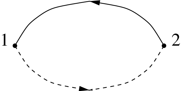
Figure 7. Order $1$.

In even dimensions, $\Theta_{1}$ furnishes a function on $\operatorname{Imb}_{\sigma}$ which is a generalization of the self-linking number for ordinary knots. This function is not an invariant. It can be easily proved that, in computing the differential of $\Theta_{1}$, the only boundary contribution corresponds to the collapse of the two points. One obtains then

$${\mathrm{d}}\Theta_{1}=-p_{1*}(\Phi^{*}w_{m-1}\;p_{3}^{*}w_{m-3}),$$

where

$$\Phi\colon\begin{array}[t]{ccc}\operatorname{Imb}_{\sigma}\times{\mathbb{R}}^{m-2}\times S^{m-3}&\to&S^{m-1}\\ (f,x,v)&\mapsto&\frac{{\mathrm{d}}f(x)v}{\left\lvert\!\left\lvert{\mathrm{d}}f(x)v\right\rvert\!\right\rvert}\end{array}$$

and $p_{i}$ denotes the projection to the $i$th factor.

6.2. Order $2$

The contributions corresponding to connected diagrams may be written as $\Theta_{2}\operatorname{Tr}((\operatorname{ad}\Xi)^{2})$, where $\Theta_{2}$ is graphically represented in fig. 8 (where white circles denote vertices in ${\mathbb{R}}^{m}$ not constrained to lie on the image of the imbedding) and has the following analytical expression:

(6.3) $$\Theta_{2}=\int_{C_{4,0}}\theta_{13}\theta_{24}\eta_{12}\eta_{23}+\frac{1}{2}\int_{C_{4,0}}\theta_{13}\theta_{24}\eta_{12}\eta_{34}-\int_{C_{3,1}}\theta_{14}\theta_{24}\theta_{34}\eta_{12}.$$

Figure 8. Order $2$.

It is not difficult to prove that $\Theta_{2}$ vanishes if $m$ is even (consider the involutions that exchange point $1$ with point $3$ in the first term, point $1$ with point $2$ in the last term, and the pair of points $(1,3)$ with the pair $(2,4)$ in the second term). In odd dimensions, $\Theta_{2}$ may be rewritten as

$$\Theta_{2}=\frac{1}{8}\int_{C_{4,0}}\theta_{13}\theta_{24}\eta_{1234}^{2}-\frac{1}{3}\int_{C_{3,1}}\theta_{14}\theta_{24}\theta_{34}\eta_{123},$$

where $\eta_{1234}$ and $\eta_{123}$ are the cyclic sums

$$\eta_{1234}=\eta_{12}+\eta_{23}+\eta_{34}+\eta_{41},\quad\eta_{123}=\eta_{12}+\eta_{23}+\eta_{31}.$$

In this form it is clear that $\Theta_{2}$ is the long-knot version of the invariant of knots introduced by Bott in [2].

Proposition 6.2.

$\Theta_{2}$ is an invariant.

Proof.

In the computation of ${\mathrm{d}}\Theta_{2}$, the contributions of the principal faces of the three terms cancel each other as can be easily verified. The vanishing of hidden faces may be easily proved, see [14]. ∎

6.3. Order $3$

Connected diagrams sum up to yield a term of the form $\Theta_{3}\operatorname{Tr}((\operatorname{ad}\Xi)^{3})$—which clearly vanishes if the Lie algebra is unimodular—where $\Theta_{3}$ corresponds to the sum of the eight Feynman diagrams displayed in fig. 9. Its analytical expression is the following:

(6.4) $$\Theta_{3} =\frac{1}{3}\int_{C_{6,0}}\theta_{14}\theta_{26}\theta_{35}\eta_{12}\eta_{34}\eta_{56}+\int_{C_{6,0}}\theta_{14}\theta_{26}\theta_{35}\eta_{12}\eta_{23}\eta_{45}+$$

$$\phantom{=}-\int_{C_{6,0}}\theta_{14}\theta_{26}\theta_{35}\eta_{12}\eta_{23}\eta_{34}+\frac{1}{3}\int_{C_{6,0}}\theta_{14}\theta_{25}\theta_{36}\eta_{12}\eta_{23}\eta_{31}+$$

$$\phantom{=}+\int_{C_{5,1}}\theta_{16}\theta_{36}\theta_{56}\theta_{24}\eta_{12}\eta_{34}-\int_{C_{5,1}}\theta_{16}\theta_{36}\theta_{56}\theta_{24}\eta_{12}\eta_{23}+$$

$$\phantom{=}-\int_{C_{4,2}}\theta_{16}\theta_{36}\theta_{56}\theta_{25}\theta_{45}\eta_{12}+\frac{1}{3}\int_{C_{3,3}}\theta_{14}\theta_{25}\theta_{36}\theta_{45}\theta_{46}\theta_{56}.$$

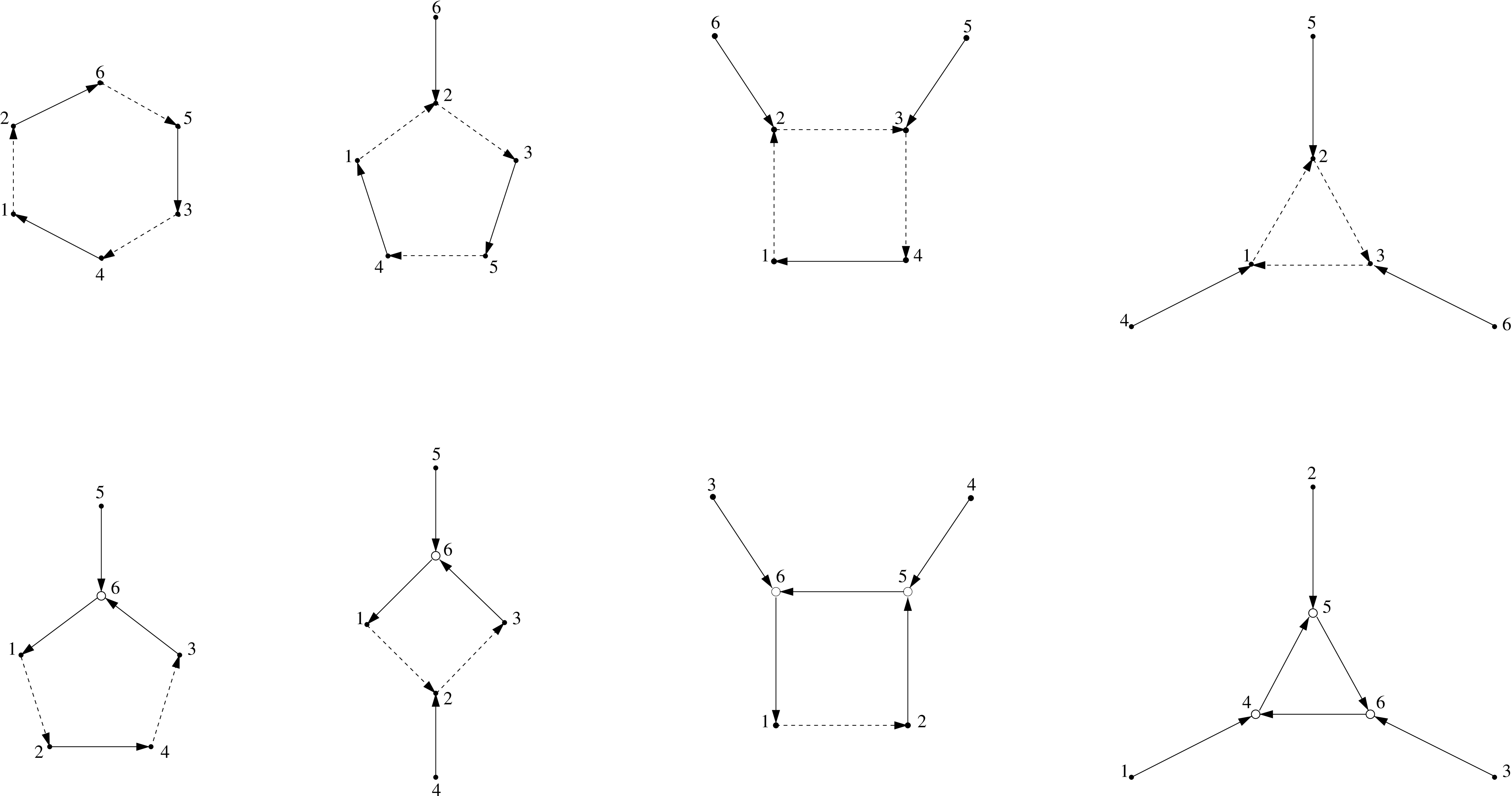
Figure 9. Order $3$.

In [14] it is proved (by considering suitable involutions) that $\Theta_{3}$ vanishes if $m$ is odd.

In even dimensions, the differential of $\Theta_{3}$ is explicitly computed in [14] and it is proved that the only boundary contribution that may survive in each term is the most degenerate face, i.e., the one corresponding to the collapse of all vertices (and with some more effort it is moreover proved that only the seventh term may yield a nonvanishing contribution). To describe ${\mathrm{d}}\Theta_{3}$, we first introduce the space $\mathcal{I}_{m,m-2}$ of linear injective maps from ${\mathbb{R}}^{m-2}$ into ${\mathbb{R}}^{m}$. Next we consider the map

$$T\colon\begin{array}[t]{ccc}\operatorname{Imb}_{\sigma}\times{\mathbb{R}}^{m-2}&\to&\mathcal{I}_{m,m-2}\\ (f,x)&\mapsto&{\mathrm{d}}f(x)\end{array}$$

Then we may write

$${\mathrm{d}}\Theta_{3}=p_{1*}T^{*}\widehat{\Theta}_{3},$$

where $p_{1}$ is the projection onto the first factor and the “anomaly” $\widehat{\Theta}_{3}$ is an $(m-1)$-form that can be explicitly described as follows. Given $\alpha\in\mathcal{I}_{m,m-2}$, one defines the following action on $C_{s,t}(\alpha)$ of the group $I={\mathbb{R}}^{+}_{*}\ltimes{\mathbb{R}}^{m-2}$ of dilations and translations of ${\mathbb{R}}^{m-2}$:

$$x_{i}\mapsto\lambda x_{i},\ i=1,\dots,s,\quad y_{i}\mapsto\lambda y_{i},\ i=1,\dots,t,\qquad\lambda\in{\mathbb{R}}^{+}_{*},$$

$$x_{i}\mapsto x_{i}+a,\ i=1,\dots,s,\quad y_{i}\mapsto y_{i}+\alpha(a),\ i=1,\dots,t,\qquad a\in{\mathbb{R}}^{m-2}.$$

One then defines $\widehat{C}_{s,t}(\alpha)$ as the quotient of $C_{s,t}(\alpha)$ by $I$. Denoting by $\widehat{C}_{s,t}^{m,m-2}\to\mathcal{I}_{m,m-2}$ the fiber bundle with fiber $\widehat{C}_{s,t}(\alpha)$ over $\alpha$, one may write $\widehat{\Theta}_{3}$ as a sum of integrals along the fibers of $\widehat{C}_{s,t}^{m,m-2}$ where the integrand form is given by the same products of propagators $\eta_{ij}$ and $\theta_{ij}$ as before, with the only modification that $\varpi_{ij}$, see (6.1), is now defined in terms of the linear map $\alpha$ (instead of $f$), over which the fiber lies.

In general, we do not know if $\Theta_{3}$ is an invariant. We briefly describe however a possible strategy to correct it.

Let $V_{m,m-2}$ be the Stiefel manifold (regarded as the space of linear isometries from ${\mathbb{R}}^{m-2}$ into ${\mathbb{R}}^{m}$ w.r.t. the Euclidean metrics). Observe that $V_{m,m-2}$ is equipped with a left action of $SO(m)$ and a free, right action of $SO(m-2)$. Let us denote by $\iota$ the inclusion of $V_{m,m-2}$ into $\mathcal{I}_{m,m-2}$ and by $r$ some deformation retract; viz., $r$ is a map from $\mathcal{I}_{m,m-2}$ to $V_{m,m-2}$ such that $\iota\circ r$ is homotopic to the identity (the existence of such a retract may be proved, e.g., by Gram–Schmidt orthogonalization procedure). Let $h$ be a given homotopy, i.e., a map $[0,1]\times\mathcal{I}_{m,m-2}\to\mathcal{I}_{m,m-2}$ such that $h(0,\alpha)=\alpha$ and $h(1,\alpha)=\iota(r(\alpha))$. Define

$$\widetilde{\Theta}_{3}=\mathit{pr}_{2*}h^{*}\widehat{\Theta}_{3},$$

where $\mathit{pr}_{2}$ denotes the projection onto the second factor. Given the explicit form of $\widehat{\Theta}_{3}$, one can prove that it is closed. Thus, we obtain

$${\mathrm{d}}\widetilde{\Theta}_{3}=-\widehat{\Theta}_{3}+r^{*}\iota^{*}\widehat{\Theta}_{3}.$$

It is now possible to show that $\boldsymbol{\Theta}_{3}:=\iota^{*}\widehat{\Theta}_{3}$ is $SO(m-2)\times SO(m)$-invariant. If $m=4$, we can moreover prove that $\boldsymbol{\Theta}_{3}$ is also $SO(m-2)$-horizontal; hence it is the pullback of an $SO(4)$-invariant $3$-form on the Grassmannian $\mathit{Gr}_{4,2}$. Since the only such form is zero, it follows that in four dimensions $\boldsymbol{\Theta}_{3}=0$ and we get the following

Proposition 6.3.

$\overline{\Theta}_{3}:=\Theta_{3}+p_{1*}T^{*}\widetilde{\Theta}_{3}$ is an invariant of long $2$-knots.

As far as we know, this invariant is new.

Observe that also for $m>4$ one may define $\overline{\Theta}_{3}$. It turns out from the previous considerations that ${\mathrm{d}}\overline{\Theta}_{3}=p_{1*}T^{*}r^{*}\boldsymbol{\Theta}_{3}$. Thus, though in general we cannot claim that $\overline{\Theta}_{3}$ is an invariant, we can compute its differential in terms of an invariant form on the Stiefel manifold. This implies that, when ${\mathrm{d}}\overline{\Theta}_{3}$ does not vanish, we may use it to correct the potential invariants coming from higher-orders in perturbation theory, as explained in the next subsection.

6.4. Higher orders

Higher-order terms may be explicitly computed. In [14] some vanishing Lemmata are proved which imply that only the most degenerate faces (i.e., when all points collapse) contribute to the differential of the corresponding functions on $\operatorname{Imb}_{\sigma}$. One can then prove that in odd dimensions also these contributions vanish. One then obtains genuine invariants of long $(m-2)$-knots with $m$ odd.

In even dimensions, one may repeat the considerations of the previous subsection. In particular, in four dimensions one may construct genuine invariants of long $2$-knots. For $m>4$, this construction yields an infinite set of functions on $\operatorname{Imb}_{\sigma}$ whose differentials are pullbacks of $SO(m-2)\times SO(m)$-invariant $(m-1)$-forms on $V_{m,m-2}$. Since the space of such forms is finite dimensional [12], one may produce an infinite set of invariants by taking suitable linear combinations. This is the higher-dimensional analogue of the procedure used in [3] to kill the (possible) anomalies in the perturbative expansion of Chern–Simons theory with covariant gauge fixing.

6.5. Other observables

The new observable we have introduced in this paper is not the only known observable for $BF$ theories. For example, the usual Wilson loop

$$W_{\rho}(\gamma)(A)=\operatorname{Tr}(\rho(\mathrm{Hol}(A,\gamma)),$$

where $\rho$ is a representation of the Lie group $G$ and $\gamma$ an imbedding of $S^{1}$, is an observable; more generally, one also has the generalized Wilson loops introduced in [7, 9], whose expectation values yield cohomology classes on the space of imbeddings of $S^{1}$.

The expectation value of the usual Wilson loop is rather trivial (the dimension of the representation space) since the degree in ${\mathsf{a}}$ cannot be matched by the degree in ${\mathsf{B}}$. The mixed expectation value of ${\mathsf{U}}_{0}$ and $W_{\rho}$ is more interesting. If $\gamma$ does not intersect $f$, the product defines an observable, and one can show that

(6.5) $${\left\langle\;{{\mathsf{U}}_{0}(f)\,W_{\rho}(\gamma)}\;\right\rangle}={\left\langle\;{{\mathsf{U}}_{0}(f)}\;\right\rangle}\,\operatorname{Tr}{\mathrm{e}}^{-\hbar\operatorname{lk}(f,\gamma)\,\rho_{*}(\Xi)},$$

where $\rho_{*}$ is the induced representation of ${\mathfrak{g}}$ and $\operatorname{lk}(f,\gamma)$ is the linking number between (the images of) $f$ and $\gamma$. It can be written as

$$\operatorname{lk}(f,\gamma)=\int_{{\mathbb{R}}^{m-2}\times S^{1}}\varphi^{*}\theta_{12}$$

where

$${\varphi}\colon\begin{array}[t]{ccc}{{\mathbb{R}}^{m-2}\times S^{1}}&\to&{C_{2}({\mathbb{R}}^{m})}\\ {(x,t)}&\mapsto&{(f(x),\gamma(t))}\end{array}$$

The result in (6.5) is tantamount saying that the only connected diagram arising from the $n$th order in $W_{\rho}$ expanded in powers of $a$ is the one obtained by joining each of these $n$ $a$s to a short snake $\sigma_{0}$. This result is purely combinatorial after observing that either joining the last ${\mathsf{a}}$ of a snake to the ${\mathsf{B}}$ of a $\sigma_{0}$ or joining the two ${\mathsf{a}}$s of an interaction vertex to the ${\mathsf{B}}$s of two $\sigma_{0}$s yields a factor ${\left[{\,{\Xi}\,,\,{\Xi}\,}\right]}$ which clearly vanishes.

7. Final comments

In this paper we have introduced a new observable for $BF$ theories that is associated to imbeddings of codimension two. We list here some possible follow-ups of our work.

7.1. Yang–Mills theory

In [4], Yang–Mills theory is regarded as a deformation, called $BF$YM theory, of $BF$ theory with deformation parameter the coupling constant $g_{\text{YM}}$. In this setting $\mathcal{O}(A,B,f)$ becomes an observable for the $BF$YM theory in the topological limit $g_{\text{YM}}\to 0$. Moreover, in this limit the expectation value of this observable times a Wilson loop is still given by (6.5). Thus, $\mathcal{O}$ might constitute the topological limit of a dual ’t Hooft variable [17].

7.2. Nonabelian gerbes

Assume $B$ to be a two form (in the context of $BF$ theories, we assume then that we are working in four dimensions). In the abelian case, the observable (1.1) defines a connection for the gerbe defined by $B$ [16]; in this case, it is interesting to consider also the case when $N$ has boundary. A suitable extension of our observable $\mathcal{O}$ to this case would then be a candidate for a connection on a nonabelian gerbe.

7.3. Classical Hamiltonian viewpoint

For $M$ of the form $M_{0}\times{\mathbb{R}}$, the reduced phase space of $BF$ theory is the space of pairs $(A,B)$, with $A$ a flat connection on $M_{0}$ and $B$ a covariantly closed $(m-2)$-form of the coadjoint type, modulo symmetries. The Poisson algebra generated by generalized Wilson loops is considered in [8] and, in the case $G=GL_{n}$ it is proved to be related to the Chas–Sullivan string topology [11]. It would be interesting to see which new structure one may obtain by considering the Poisson algebra generated by generalized Wilson loops and, in addition, our new observables.

7.4. Cohomology classes of imbeddings of even codimension

In Section 6 we have described how the perturbative expansion produces (potential) invariants of long knots. The same formulae may be used to define forms on the space of imbeddings $\operatorname{Imb}_{\sigma}^{s}$ of ${\mathbb{R}}^{m-2s}$ into ${\mathbb{R}}^{m}$ (with fixed linear behavior $\sigma$ at infinity) with $s>1$; up to hidden faces, these forms are closed (they certainly are so for $m$ odd). This way, we produce cohomology classes on $\operatorname{Imb}_{\sigma}^{s}$.

7.5. Graph cohomology

Generalizing [5], one can define a graph cohomology for graphs with two types of vertices (corresponding to points on the imbedding and in the ambient space) and two types of edges (corresponding to the two types of propagators) such that the “integration map” that associates to a graph the corresponding integral over configuration spaces is a chain map up to hidden faces. The Feynman diagrams discussed in this paper produce then nontrivial classes in this graph cohomology. We plan to discuss all this in details in [10].

References

• [1] I. A. Batalin and G. A. Vilkovisky, “Relativistic $S$-matrix of dynamical systems with boson and fermion constraints,” Phys. Lett. 69 B, 309–312 (1977); E. S. Fradkin and T. E. Fradkina, “Quantization of relativistic systems with boson and fermion first- and second-class constraints,” Phys. Lett. 72 B, 343–348 (1978).
• [2] R. Bott, “Configuration spaces and imbedding invariants,” in Proceedings of the 4th Gökova Geometry–Topology Conference, Tr. J. Math. 20, 1–17 (1996).
• [3] R. Bott and C. Taubes, “On the self-linking of knots,” J. Math. Phys. 35, 5247–5287 (1994).
• [4] A. S. Cattaneo, P. Cotta-Ramusino, F. Fucito, M. Martellini, M. Rinaldi, A. Tanzini and M. Zeni, “Four-dimensional Yang–Mills theory as a deformation of topological $BF$ theory,” Commun. Math. Phys. 197, 571–621 (1998).
• [5] A. S. Cattaneo, P. Cotta-Ramusino and R. Longoni, “Configuration spaces and Vassiliev classes in any dimension,” math.GT/9910139.
• [6] A. S. Cattaneo, P. Cotta-Ramusino and M. Rinaldi, “Loop and path spaces and four-dimensional $BF$ theories: connections, holonomies and observables,” Commun. Math. Phys. 204, 493–524 (1999).
• [7] A. S. Cattaneo, P. Cotta-Ramusino and C. A. Rossi, “Loop observables for $BF$ theories in any dimension and the cohomology of knots”, Lett. Math. Phys. 51, 301–316 (2000).
• [8] A. S. Cattaneo, J. Fröhlich and B. Pedrini, “Topological field theory interpretation of string topology,” math.GT/0202176.
• [9] A. S. Cattaneo and C. A. Rossi, “Higher-dimensional $BF$ theories in the Batalin–Vilkovisky formalism: the BV action and generalized Wilson loops,” Commun. Math. Phys. 221, 591–657 (2001).
• [10] A. S. Cattaneo and C. A. Rossi, “Configuration space invariants of higher dimensional knots,” in preparation.
• [11] M. Chas and D. Sullivan, “String topology,” math/9911159.
• [12] W. Greub, S. Halperin and R. Vanstone, Connections, Curvature and Cohomology. Vol. II: Lie Groups, Principal Bundles, Characteristic Classes, Pure and Applied Mathematics 47 II, Academic Press (New York–London, 1973).
• [13] M. Kontsevich, “Feynman diagrams and low-dimensional topology,” First European Congress of Mathematics, Paris 1992, Volume II, Progress in Mathematics 120, Birkhäuser (Basel, 1994), 97–121.
• [14] C. Rossi, Invariants of Higher-Dimensional Knots and Topological Quantum Field Theories, Ph. D. thesis, Zurich University 2002, http://www.math.unizh.ch/$\sim$asc/RTH.ps
• [15] A. S. Schwarz, “The partition function of degenerate quadratic functionals and Ray–Singer invariants,” Lett. Math. Phys. 2, 247–252 (1978).
• [16] G. Segal, “Topological structures in string theory,” Phil. Trans. R. Soc. Lond. A 359, 1389–1398 (2001).
• [17] G. ’t Hooft, “On the phase transition towards permanent quark confinement,” Nucl. Phys. B 138, 1 (1978); “A property of electric and magnetic flux in nonabelian gauge theories,” Nucl. Phys. B 153, 141 (1979).
• [18] E. Witten, “Quantum field theory and the Jones polynomial,” Commun. Math. Phys. 121, 351–399 (1989).