Abstract

We present a numerical study of the nonlinear system of $\Phi^{4}_{0}$ equations of motion. The solution is obtained iteratively, starting from a precise point-sequence of the appropriate Banach space, for small values of the coupling constant. The numerical results are in perfect agreement with the main theoretical results established in a series of previous publications.

1 Introduction

1.1 A new non perturbative method

Several years ago we started a program for the construction of a non trivial $\Phi^{4}_{4}$ model consistent with the general principles of a Wightman Quantum Field Theory (Q.F.T.) [1]. In references [2] we have introduced a non perturbative method for the construction of a non trivial solution of the system of the $\Phi^{4}$ equations of motion for the Green’s functions, in the Euclidean space of zero, one and two dimensions. In references [3] we applied an extension of this method to the case of four (and a fortiori of three)-dimensional Euclidean momentum space.

This method is different in approach from the work done in the Constructive Q.F.T. framework of Glimm–Jaffe and others [4], and the methods of Symanzik who created the basis for a pure Euclidean approach to Q.F.T. [5].

It is based on the proof of the existence and uniqueness of the solution of the corresponding infinite system of dynamical equations of motion verified by the sequence of the Schwinger functions. This solution is obtained inside a particular subset characterised by alternating signs and “splitting” or factorization properties.

The reasons that motivated us for a study in smaller dimensions and not directly in four, were the absence of the difficulties due to the renormalization and the pure combinatorial character of the problem in zero dimensions.

Another useful aspect of the zero dimensional case is the fact that it provides a direct way to test numerically the validity of the method.

In a more recent work [6] a numerical analysis of the $\Phi^{4}_{0}$ solution has been obtained following our method.

This paper constitutes a new version of this work. More precisely we present the numerical study and construction of the solution of the $\Phi^{4}$ zero-dimensional problem realized by iteration. Our numerical results are coherent with our basic theorems. More precisely:

1. The validity of the contractivity criterion by the iterated mapping ${\mathcal{M}}^{*}$, is verified up to the value $\Lambda=0.01$ for the coupling constant. The calculations give an indication that it should be true beyond this value, the limit being below $0.05$ with the relaxation method used here. An unstable behaviour appears with amplified oscillations for bigger values of the coupling constant.

2. The “good” properties of “alternating signs” and “splitting” are certainly verified by the constructed solution (truncated sequence $H$).

3. When the coupling constant increases beyond the critical value $\Lambda=0.05$, the number of iterations needed for the convergence $\nu_{\rm conv}$ grows rapidly and the stability of the Green’s functions in a finite time is ensured only for a reduced number of Green’s functions

1.2 The existence and uniqueness of the $\Phi^{4}_{0}$ solution.
The theoretical background

1.2.1 The vector space ${\mathcal{B}}$ and the $\Phi^{4}_{0}$ equations of motion

Definition 1 (The space ${\mathcal{B}}$).

We consider the vector space ${\mathcal{B}}$ of the sequences $H=\{H^{n+1}\}_{n=2k+1;k\in\mathbb{N}}$ by the following:

The functions $H^{n+1}$ belong to the space $C^{\infty}(\mathbb{R}^{+})$ of continuously differentiable numerical functions of the variable $\Lambda\in\mathbb{R}^{+}$ (which physically represents the coupling constant).

Moreover, there exists a universal (independent of n and of $\Lambda$) positive constant $K_{0}$, such that the following uniform bounds are verified:

$$\forall\;n=2k+1,\ k\in\mathbb{N}\qquad\left|H^{n+1}(\Lambda)\right|\leq n!(K_{0})^{n}\qquad\forall\;\Lambda\in\mathbb{R}^{+}.$$ (1)

We suppose that the system of equations under consideration, concerns the sequences of Euclidean connected and amputated with respect to the free propagators Green’s functions (the Schwinger functions). and that these sequences denoted by $H=\{H^{n+1}\}_{n=2k+1,k\in\mathbb{N}}$ belong to the above space ${\mathcal{B}}$.

Taking into account the facts that in the present zero-dimensional case all the external four-momenta are set equal to zero, that the physical mass can be taken equal to $1$ and that the renormalization parameters must be set equal to their trivial values one directly obtains the corresponding infinite system of equations of motion for the sequence of the Schwinger functions in the following form:

$$\forall\;\Lambda\in\mathbb{R}^{+}\qquad H^{2}(\Lambda)=-\Lambda H^{4}(\Lambda)+1$$ (2)

and for all $n\geq 3$,

$$H^{n+1}(\Lambda)=A^{n+1}(\Lambda)+B^{n+1}(\Lambda)+C^{n+1}(\Lambda)$$ (3)

with:

$$A^{n+1}(\Lambda)=-\Lambda H^{n+3}(\Lambda);$$ (4)

$$B^{n+1}(\Lambda)=-3\Lambda\sum_{\varpi_{n}(J)}\frac{n!}{j_{1}!j_{2}!}H^{j_{2}+2}(\Lambda)H^{j_{1}+1}(\Lambda);$$ (5)

$$C^{n+1}(\Lambda)=-6\Lambda\sum_{\varpi_{n}(I)}\frac{n!}{i_{1}!i_{2}!i_{3}!\sigma_{\rm sym}(I)}\prod_{l=1,2,3}H^{i_{l}+1}(\Lambda).$$ (6)

1.2.2 The subset $\Phi\subset{\mathcal{B}}$ and the new contractive mapping ${\mathcal{M}^{*}}$

Definition 2.

We introduce the class ${\mathcal{D}}$ of sequences

$$\delta=\{\delta_{n}\}_{n=2k+1;k\in\mathbb{N}}\in{\mathcal{B}},$$

such that they verify the bounds (1) in the following simpler form:

$$|\delta_{n}(\Lambda)|\leq K_{0}\qquad\forall\;\Lambda\in\mathbb{R}^{+},\qquad\forall\;n=2k+1;\ k\in\mathbb{N}.$$ (7)

Definition 3 (Signs and splitting).

A sequence $H\in{\mathcal{B}}$ belongs to the subset $\Phi\subset{\mathcal{B}}$ if there exists a slowly increasing associated sequence of positive and bounded functions on $\mathbb{R}^{+}$,

$$\delta=\{\delta_{n}\}_{n=2k+1;k\in\mathbb{N}}\in{\mathcal{D}},$$

such that the following “splitting” (or factorization) and sign properties are verified $\forall\;\Lambda\in\mathbb{R}^{+}$:

$$\Phi.1\ \ H^{2}(\Lambda)=1+\Lambda\delta_{1}(\Lambda),\quad\mbox{with:}\ \ \lim_{\Lambda\rightarrow 0}\delta_{1}(\Lambda)=0;$$ (8)

$$\Phi.2\ \ H^{4}(\Lambda)=-\delta_{3}(\Lambda)\left[H^{2}(\Lambda)\right]^{3},\quad\mbox{with:}\ \ \delta_{3}(\Lambda)\leq 6\Lambda,\ \ \lim_{\Lambda\rightarrow 0}\frac{\delta_{3}(\Lambda)}{\Lambda}=6;$$ (9)

$$\Phi.3\ \ \forall\;n\geq 5\qquad H^{n+1}(\Lambda)=\frac{\delta_{n}(\Lambda)C^{n+1}}{3\Lambda n(n-1)},\quad\mbox{with:}\ \ \lim_{\Lambda\rightarrow 0}\frac{\delta_{n}(\Lambda)}{\Lambda}=3n(n-1).$$ (10)

Moreover $\exists$ a uniform bound at infinity $\delta_{\infty}^{\Lambda}$ such that:

$$\lim_{n\rightarrow\infty}\delta_{n}(\Lambda)\leq\delta_{\infty}^{\Lambda}.$$ (11)

Definition 4 (The new contractive mapping ${\mathcal{M}^{*}}$).

We define the following application ${\mathcal{M}^{*}}:\Phi\stackrel{{\scriptstyle\mathcal{M}^{*}}}{{\longrightarrow}}{\mathcal{B}}$ by:

$$H^{2^{\prime}}(\Lambda)=1+\Lambda\delta_{1}^{{}^{\prime}}(\Lambda)\qquad\mbox{with}\qquad\delta_{1}^{{}^{\prime}}(\Lambda)=-H^{4}(\Lambda),$$ (12)

$$H^{4^{\prime}}(\Lambda)=-\delta_{3}^{{}^{\prime}}(\Lambda)\left[H^{2^{\prime}}\right]^{3}\quad\mbox{with}\quad\delta_{3}^{{}^{\prime}}(\Lambda)=6\Lambda\!\left[1+6\Lambda H^{2}\!\left(\frac{3}{2}-\frac{\left|H^{6}\right|}{6\left|H^{4}\right|\left|H^{2}\right|}\right)\!\right]^{-1}\!\!\!\!\!\!\!$$ (13)

and for every $n\geq 5$

$$H^{n+1^{\prime}}(\Lambda)=\frac{\delta_{n}^{{}^{\prime}}(\Lambda)C^{n+1^{\prime}}(\Lambda)}{3\Lambda n(n-1)};$$ (14)

with:

$$\delta_{n}^{{}^{\prime}}(\Lambda)=\frac{3\Lambda n(n-1)}{1+D_{n}(H)}$$ (15)

and

$$D_{n}(H)=\frac{\left|B^{n+1}\right|-\left|A^{n+1}\right|}{\left|H^{n+1}\right|}.$$ (16)

Theorem 1

(The contractivity of the mapping ${\mathcal{M}^{*}}$ inside $\Phi$ and the construction of the unique non trivial $\Phi_{0}^{4}$ solution.)

1. The subset $\Phi$ is a nonempty, closed, complete subspace of ${\mathcal{B}}$ in the induced topology.

2. There exists a finite positive constant $\Lambda^{*}(\approx 0.01)$ such that the mapping ${\mathcal{M}^{*}}$ is contractive inside the subset $\Phi$ and therefore the mapping ${\mathcal{M}}$ has a unique nontrivial fixed point inside the subset $\Phi$ when $\Lambda\in]0,\Lambda^{*}]$.

3. The unique nontrivial solution of the $\Phi_{0}^{4}$ equations of motion lies in a neihbourhood of the fundamental sequence $H_{0}$.

2 The numerical study of the $\Phi^{4}_{0}$ solution

2.1 The algorithm for the numerical construction of the $\Phi^{4}_{0}$ solution

2.1.1 The iterative procedure

For the numerical realization of the solution of the system, we applied the following iterative procedure: We considered the so called “fundamental sequence” $H_{0}$ mentioned in the previous section. We have chosen it because:

1. It has a simple form which “imitates” the mapping.

2. It is a nontrivial point of the appropriate subset $\Phi$ (validity of the signs and splitting properties) where we have shown that the solution is expected to be.

For these two reasons we could expect a rapid convergence of the iteration to the solution in the neighbourhood of this sequence $H_{0}$:

$$H^{2}_{0}(\Lambda)=1+6\Lambda^{2},$$ (17)

$$H^{4}_{0}(\Lambda)=-6\Lambda\left[H^{2}_{0}(\Lambda)\right]^{3},$$ (18)

and $\forall\;n\geq 5$

$$H^{n+1}_{0}(\Lambda)=\frac{\delta_{n,0}(\Lambda)C^{n+1}_{0}(\Lambda)}{3\Lambda n(n-1)},$$ (19)

with:

$$C^{n+1}_{0}(\Lambda)=-6\Lambda\sum_{\varpi_{n}(I)}\frac{n!}{i_{1}!i_{2}!i_{3}!\sigma_{\rm sym}(I)}\prod_{l=1,2,3}H^{i_{l}+1}_{0}(\Lambda)$$ (20)

and

$$\delta_{n,0}(\Lambda)=\frac{3\Lambda n(n-1)}{1+0.5\Lambda n\ (n-1)}.$$ (21)

Then, taking this sequence as starting point we iterated the zero-dimensional analog of the mapping ${\mathcal{M}}^{*}$, precisely Definition 16.

2.1.2 Convergence and stopping criteria

Let us first introduce the following definitions:

1. The “dimension” of each truncated sequence $H$ used by the computer denoted by $n_{\max}$.

2. The sequence $H_{\rm conv}$ which is characterized by all components taken at their convergence values.

3. The sequence $\delta_{\rm conv}$ which is the splitting sequence associated with $H_{\rm conv}$.

For some given value of the coupling constant $\Lambda$ and $n_{\max}$, the algorithm calculates by iteration the values of $H$ (that means all the components $H^{n+1}$, for $1\leq n\leq n_{\max}$), and stops when the value nearly does not vary between a step and the next one, using the following criteria (independently on each component of $H$):

• near $0$, (if $\left|H^{n+1}_{\rm conv}\right|\leq\epsilon_{H}$) the convergence is obtained if

  $$\left|H^{n+1}-H^{n+1}_{\rm conv}\right|<\epsilon_{H};$$

• otherwise, by using the value $\epsilon_{H}=10^{-10}$ we apply the relative criterium

  $$\left|\frac{H^{n+1}}{H^{n+1}_{\rm conv}}-1\right|<\epsilon_{H}.$$

When for one component of $H$ the convergence is obtained, the value of $H^{n+1}_{\rm conv}$ is frozen, and the order of iteration is memorized as $\nu_{\rm conv}$. When the convergence is obtained for all the components of $H$, the algorithm stops, the values of $H_{\rm conv}$ and $\nu_{\rm conv}$ are memorized, and the values of $\delta$ are memorized as $\delta_{\rm conv}$. To avoid an infinite loop, a maximum number of iterations is also given. Then, the algorithm also stops, and the same values are memorized, but they are only the last obtained values, not the convergence ones, since the convergence was not obtained.

2.2 Graphical representations and conclusions

2.2.1 The $H$’s and $\delta$’s as functions of $\nu$

We have chosen to realize the computation for $n_{\max}=55$ and $10$ values of $\Lambda$ from $0.010$ to $0.100$ because:

• Some phenomena do not appear for small values of $n_{\max}$. For example if $n_{\max}\leq 29$ roughly, the convergence is obtained for much bigger values of $\Lambda$ and the oscillations are not observed.

• For bigger values of $n_{\max}$ the needed time and memory space become prohibitive for our machines.

We obtained the values of $H^{n+1}$’s and $\delta_{n}$’s as functions of $\nu$ (the order of iteration) for some given $n_{\max}$ and $\Lambda$. The $H^{n+1}$’s themselves have (as expected by the method) alternately positive $\left(H^{2},H^{6},H^{10},\ldots\right)$ and negative $\left(H^{4},H^{8},H^{6},\ldots\right)$ signs (except in the case of divergence). We find that $H^{2}$ converges towards values a little greater than $1$, (as it was expected theoretically).

The curves giving $H^{n+1}$’s are very flat, and what happens is most clear when we analyse the curves giving the $\delta_{n}$’s (“splitting”sequences):

For small values of $\Lambda$, the algorithm converges monotonically (Fig. 1), but damped oscillations appear (starting from the value $0.020$) for bigger values of $\Lambda$. An approximated pseudo-period can be found. It is roughly linearly linked to the “dimension” of the space, because of the perturbations due to the particular form of the mapping.

When $\Lambda$ increases, the oscillations are less and less damped, very slightly damped for $0.050$ (Fig. 2), and then amplified, more and more, and remain with a smaller and less stable pseudo-period, before explosion. These oscillations do not appear if $n_{\max}\leq 29$ roughly, or $\Lambda$ very big. In the latter case the divergence occurs before the end of the first pseudo-period.

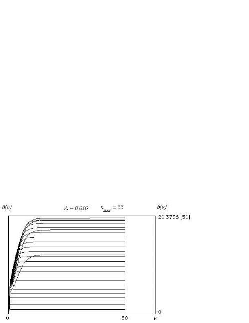
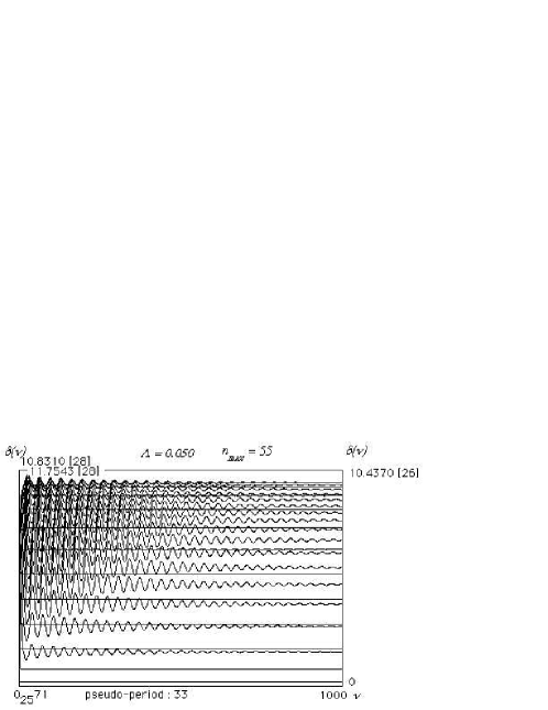
Figure 1: Convergence of $\delta_{n;\nu}(\Lambda=0.01)$ as a function of the iteration number $\nu$ for $n_{\max}=55$.

Figure 2: Convergence of $\delta_{n;\nu}(\Lambda=0.05)$ as a function of the iteration number $\nu$ for $n_{\max}=55$.

The convergence (verification of the contractivity criterium) which has been proven mathematically up to $\Lambda=0.010$ can here be shown numerically for values slightly larger, and we can see how it is progressively destroyed, since a pronounced instability appears in the form of amplified oscillations when the coupling constant increases.

2.2.2 Curves of $H_{\rm conv}$, $\delta_{\rm conv}$ and $\nu_{\rm conv}$, as functions of $n_{\max}$

In order to keep the article down to manageable size we do not present the figures we comment here. They are, of course, at the disposal of all interested readers, in the corresponding electronic version of the journal [8].

1. For small coupling constant, $\Lambda\leq 0.03$, the curves of $H_{\rm conv}$ (i.e. the values of $H^{n+1}$’s for which the convergence is obtained) as a function of $n_{\max}$ (the dimension of the used truncated sequence) show a good convergence, for sufficiently small $n_{\max}$. But, when $n_{\max}$ increases, analogous instabilities appear again: there are damped oscillations, then amplified oscillations and there is no more convergence. Just before the threshold of this phenomenon, the number of iterations needed for the convergence grows very rapidly.

2. The curves of $\delta_{\rm conv}$ (i.e. the corresponding $\delta_{n}$’s of the iteration for which the convergence is obtained) as a function of $n_{\max}$, show similar properties of the iteration procedure. For small values of the coupling constant the convergence is obtained (for both the $\delta_{n}$’s and the enveloppe of the curves) as far as $n_{\max}$ increases.

   For $\Lambda=0.01$, no instability appears up to $n_{\max}=119$ (with a limit of $200$ iterations), and the maximum $\delta_{\rm conv}$ obtained can be found around $30$. For $\Lambda=0.02$, some instabilities appear for $n_{\max}$ near $90$, and for $\Lambda\geq 0.06$, they begin for $n_{\max}\leq 50$.

3. Finally, the curves representing $\nu_{\rm conv}$ (the iteration order for the convergence of each component) as a function of $n_{\max}$ make evident an analogous behaviour. Moreover, these curves yield some concrete idea about the speed of convergence of the iteration.

   For small values of the coupling constant ($\Lambda\leq 0.03$), the number of iterations needed to obtain the convergence grows roughly linearly with the dimension of the space $n_{\max}$ and the component number $n$. The first components converge rapidly and independenly of $n_{\max}$ because the different Green’s functions are very weekly coupled and reach their limit value before the truncation number ($n_{\max}$) takes his largest values.

   When the coupling constant grows ($\Lambda\geq 0.04$), the required number of iterations for the convergence, $\nu_{\rm conv}$, grows very rapidly and all the components $H^{n+1}$, but the first ones, converge simultaneously being strongly coupled between them. The convergence is no more obtained for bigger values of $n_{\max}$.

   This divergence occurs for smaller and smaller $n_{\max}$, when $\Lambda$ increases.

2.3 Outlook and further investigations

1. In order to study more precisely the behaviour of the convergence, we also obtained numerical results and curves showing the ratio

   $$\left|\frac{H^{n+1}_{\nu}}{H^{n+1}_{\nu_{\rm conv}}}\right|$$

   at fixed $\Lambda$ and $n_{\max}$. The convergence again is evident up to the values $\Lambda\leq 0.04$ ([7]). Oscillations appear from $\Lambda\geq 0.05$ and they are amplified for larger values of the coupling constant.

2. We also explored another aspect of the iteration by perfoming a kind of “map” [7] as follows.

   The iteration process starts upwards: From the $H^{2}$ Green’s function and $\Lambda$ we calculate the $H^{4},H^{6},\ldots,H^{n_{\max}+1}$ Green’s functions using the iteration formulas and we verify the sign of each of the Green’s functions. If the alternating signs (positive for $H^{2}$-negative for $H^{4},\ldots$ etc.) are obtained, that means the convergence is guaranteed. If the sign is wrong, the iteration yields values without any physical significance; then, the convergence is impossible.

3. In order to accelerate the convergence of the iteration we are looking at two types of investigations:

   • We can “redefine” each step of the iteration by putting together the calculations of $2$ steps of our previous procedure.

   • We also can define another starting point of the iteration by choosing appropriate and more physical values of the splitting sequence, in terms of the values of the coupling constant. More precisely, if instead of the fundamental sequence $H_{0}$, we take as initial point of the iteration one of the previous fixed points (at a given value of $\Lambda$ and $n_{\max}$) one expects a very rapid convergence to the physical solution without chaotic behaviour.

   These two last points are under investigation [7].

Acknowledgments

The authors are indebted to O Lanford for useful discussions and comments of previous versions of this work. They are also grateful to B Grammaticos for a critical reading of the paper and crucial remarks. The authors would like also to thank the director of EISTI, N Fintz for his encouragements and excellent conditions at EISTI during the elaboration of this work.

References

-
[1]
Wightman A S, Phys. Rev. 101 (1965), 860;
Streater R and Wightman A, PCT Spin Stat. and all That, Benjamin, New York, 1964;
Bogoliubov N N, Logunov A A and Todorov I T, Introduction to the Axiomatic Q.F.T., Benjamin, New York, 1975;
Jost R, The General Theory of Quantized Fields, American Math. Society, Providence, RI, 1965;
Bogoliubov N N and Shirkov D V, Introduction to the Theory of Quantized Fields, Interscience, New York, 1968. -
[2]
Manolessou M,
J. Math. Phys. 29 (1988), 2092;
30 (1989), 175; 30, (1989), 907;
32 (1991), 12;
Back to the Solution, Preprint E.I.S.T.I., 1994. -
[3]
Manolessou M,
Nucl. Physics B (Proc. Suppl.) 6 (1989), 163–166;
The Non Trivial Solution, Preprint E.I.S.T.I., 1992;
Contribution to the International Congress of Math. Physics, Unesco-Sorbonne, Editor: D. Iagolnitzer, 1994. -
[4]
Glimm J and Jaffe A,
Phys. Rev. 176 (1968), 1945;
Commun. Math. Phys. 11 (1968), 99;
Bull. Ann. Math. Soc. 76 (1969), 407;
Acta. Math. 125 (1970), 203;
Stat. Mech. and Quantum Field Theory, Les Houches, 1970, 1–108, Gordon and Breach, New York, 1971. - [5] Symanzik K, J. Math. Phys. 7 (1966), 510.
- [6] Gladkoff S, Alaie A, Sansonnet Y and Manolessou M, Preprint EISTI, 1995.
- [7] Gladkoff S and Manolessou M, Preprint EISTI, 2001 (in preparation).
- [8] Gladkoff S, Alaie A, Sansonnet Y and Manolessou M, J. Nonlin. Math. Phys. 9 Nr.1 (2001) (Electronic version).