Quantum Electrodynamics on the 3-torus
I.- First step

Abstract

We study the ultraviolet problem for quantum electrodynamics on a three dimensional torus. We start with the lattice gauge theory on a toroidal lattice and seek to control the singularities as the lattice spacing is taken to zero. This is done by following the flow of a sequence of renormalization group transformations. The analysis is facilitated by splitting the space of gauge fields into into large fields and small fields at each step following Balaban. In this paper we explore the first step in detail.

1 Introduction

Quantum electrodynamics in a four dimensional space time, (QED)₄, is the basic theory of electrons and photons. The theory is very singular at short distances. Nevertheless it does have a well defined perturbation theory (expansion in the coupling constant) provided various renormalizations are carried out. At this level it gives a spectacularly precise description of nature.

One would like to have a rigorous non-perturbative construction of the model. To date this has not been possible and success is not likely anytime soon. However the singularities are weaker in lower dimensions and there is the possibility of progress. In this sequence of papers we give a construction of (QED)₃. To avoid long distance (infrared) problems, which are also present, we work on the three dimensional torus.

The theory is formally defined by functional integrals. The program is to add cutoffs to take out the short distance (ultraviolet) singularities and make the theory well-defined. Then one tries to remove the cutoffs. The singularities that develop are to be cancelled by adjusting the bare parameters - this is renormalization. At the same time one must keep control throughout over the size of the functional integrals - this is the stability problem.

An effective way to deal with these difficulties is to regularize the theory by putting it on a lattice and then study the continuum limit. This regularization has the advantage of preserving gauge invariance. This helps with the treatment of the singularities- the counterterms required are minimal. The stability problem also seems more tractable in the lattice approximation.

Our general method is the renormalization group (RG) technique. We first scale up to a unit lattice theory. By block averaging we generate a sequence of effective actions corresponding to different length scales. The effective coupling constant starts from near zero and grows but remains small. Renormalization cancellations are made perturbatively at each level. The remainders must also be controlled and for this we need control over the size of the gauge field. This is accomplished by breaking the functional integral into large and small field regions at each level. The contribution of the large field region is suppressed by the free measure, and in the small field region we can do the perturbative analysis. Stability emerges naturally in this approach as well.

The scheme outlined above was originally developed by Balaban for a study of scalar (QED)₃ [1], [2], [3], [4]. See also King [21]. The method was further developed by Balaban, Brydges, Imbrie, and Jaffe [7], [8] who used it in their study of the Higgs mechanism for this model. There is further exposition of this work in lecture notes by Imbrie [20]. Balaban continued by proving basic stability bounds for pure Yang-Mills YM₃, YM₄ [5],[6]. Balaban, O’Carroll, and Schor [9], [10] gave an analysis of the fermion propagators that arise in a RG approach. These papers were the main inspiration for the present work.

Let us also mention some earlier related results. Weingarten and Challifour [25] and Weingarten [26] gave a construction of (QED)₂. For scalar electrodynamics there is extensive work for $d=2$ by Brydges, Fröhlich, and Seiler [13]. Magnen and Seneor gave a treatment of Yukawa in $d=3$ [22]. For a heuristic discussion of (QED)₃ see [14].

The present work will not directly generalize to (QED)₄. The problem is that this model lacks ultraviolet asymptotic freedom, the flow of the effective coupling constants away zero. However the present work is progress toward a construction of quantum chromodynamics (QCD)_3,4, the fundamental theory of the strong interactions. It seems likely that combining Balaban’s results on Yang-Mills [5],[6] with the present work would be sufficient, albeit still on a torus.

Acknowledgement: I would like to thank T. Balaban for helpful conversations.

2 Preliminaries

2.1 the model

The basic torus is ${\mathbb{T}}_{M}=({\mathbb{R}}/L^{M}{\mathbb{Z}})^{3}$ where $L$ is a fixed large positive number and $M\geq 0$ is a fixed nonnegative integer. It has volume $L^{3M}$. In this torus we consider lattices with spacing $L^{-N}$ defined by

$${\mathbb{T}}_{M}^{-N}=(L^{-N}{\mathbb{Z}}/L^{M}{\mathbb{Z}})^{3}$$ (1)

Let $\bar{\psi},\psi$ be fermi fields and let ${\cal A}$ be an Abelian gauge field on the lattice. The lattice version of Euclidean (QED)₃ in the Feynman gauge is defined by the density

$$\begin{split}\rho(\bar{\psi},\psi,{\cal A})=\exp\left(-\frac{1}{2}({\cal A},(-\Delta+\mu^{2}){\cal A})-(\bar{\psi},(D_{e}({\cal A})+m)\psi)-\delta v-\delta E\right)\end{split}$$ (2)

Here $D_{e}(A)$ is the lattice Dirac operator with potential ${\cal A}$ and coupling constant $e\geq 0$, and $\delta v,\delta E$ are mass and energy counterterms. We are interested in integrals like the normalization factor (partition function)

$$Z=\int\rho(\bar{\psi},\psi,{\cal A})\ d\bar{\psi}\ d\psi\ d{\cal A}$$ (3)

and in correlation functions such as the two point function

$$<\psi(x)\bar{\psi}(y)>=Z^{-1}\int\psi(x)\bar{\psi}(y)\ \rho(\bar{\psi},\psi,{\cal A})\ d\bar{\psi}\ d\psi\ d{\cal A}$$ (4)

The problem is to control the $N\to\infty$ limit.

Let us explain the terms in (2) is more detail. The gauge field ${\cal A}={\cal A}(xx^{\prime})$ is a real valued function on bonds $x,x^{\prime}$ (nearest neighbors) in ${\mathbb{T}}_{M}^{-N}$ satisfying ${\cal A}(xx^{\prime})=-{\cal A}(x^{\prime}x)$. If $\{e_{\mu}\}=\{e_{1},e_{2},e_{3}\}$ are oriented unit basis vectors we write ${\cal A}_{\mu}(x)={\cal A}(x,x+L^{-N}e_{\mu})$. The derivative of ${\cal A}_{\mu}$ in the direction $e_{\nu}$ is

$$(\partial_{\nu}{\cal A}_{\mu})(x)=({\cal A}_{\mu}(x+L^{-N}e_{\nu})-{\cal A}_{\mu}(x))/L^{-N}$$ (5)

and $({\cal A},(-\Delta+\mu^{2}){\cal A})$ is the quadratic form defined by the lattice Laplacian:

$$({\cal A},(-\Delta+\mu^{2}){\cal A})=\sum_{\mu,\nu,x}L^{-3N}|(\partial_{\nu}{\cal A}_{\mu})(x)|^{2}+\mu^{2}\sum_{\mu,x}L^{-3N}|{\cal A}_{\mu}(x)|^{2}$$ (6)

The fermion fields $\bar{\psi}_{\alpha}(x),\psi_{\alpha}(x)$ are indexed by $x\in{\mathbb{T}}_{M}^{-N}$ and $1\leq\alpha\leq 4$. They are the natural basis for the space of functions from the lattice to pairs of four component spinors. They provide a basis for the Grassman algebra generated by this space. This is the space of fermions fields. Integration over fermion fields means projection onto the element of maximal degree. The Dirac operator is given by

$$(\bar{\psi},D_{e}({\cal A})\psi)=L^{-2N}\sum_{xx^{\prime}}\bar{\psi}(x)\gamma_{xx^{\prime}}e^{ieL^{-N}{\cal A}(xx^{\prime})}\psi(x^{\prime})\ -\frac{3r}{2}L^{-2N}\sum_{x}\bar{\psi}(x)\psi(x)$$ (7)

If $x^{\prime}=x\pm L^{-N}e_{\mu}$ then then $\gamma_{xx^{\prime}}=\frac{1}{2}(r\pm\gamma_{\mu})$ where $\gamma_{\mu}$ are the usual self-adjoint Dirac matrices satisfying $\{\gamma_{\mu},\gamma_{\nu}\}=2\delta_{\mu\nu}$. This can also be written as

$$\begin{split}(\bar{\psi},D_{e}({\cal A})\psi)=&L^{-2N}\sum_{x,\mu}\bar{\psi}(x)(\frac{r+\gamma_{\mu}}{2})e^{ieL^{-N}{\cal A}(x,x+L^{-N}e_{\mu})}\psi(x+L^{-N}e_{\mu})\\ +&L^{-2N}\sum_{x,\mu}\bar{\psi}(x)(\frac{r-\gamma_{\mu}}{2})e^{ieL^{-N}{\cal A}(x,x-L^{-N}e_{\mu})}\psi(x-L^{-N}e_{\mu})\\ -&\frac{3r}{2}L^{-2N}\sum_{x}\bar{\psi}(x)\psi(x)\\ \end{split}$$ (8)

Formally the $r$ terms disappear as $N\to\infty$ and we get the usual continuum action $\sum_{\mu}\int\bar{\psi}(x)\gamma_{\mu}(\partial_{\mu}+ie{\cal A}_{\mu}(x))\psi(x)dx$. The propagator for this action has some well-known pathologies when $r=0$, so we take a fixed $0<r\leq 1$.

Actually we want a modification of the above corresponding to anti-periodic boundary conditions for the fermions. Instead of basis vectors $\bar{\psi}(x),\psi(x)$ indexed by the torus ${\mathbb{T}}_{M}^{-N}$ we consider basis vectors $\bar{\psi}(x),\psi(x)$ indexed by the infinite lattice $(L^{-N}{\mathbb{Z}})^{3}$, but with the identifications

$$\begin{split}\psi(x+L^{M}e_{\mu})=&-\psi(x)\\ \bar{\psi}(x+L^{M}e_{\mu})=&-\bar{\psi}(x)\\ \end{split}$$ (9)

Then $j(x,x^{\prime})\equiv\bar{\psi}(x)\gamma_{xx^{\prime}}e^{ieL^{-N}{\cal A}(xx^{\prime})}\psi(x^{\prime})$ satisfies $j(x+L^{M}e_{\mu},x^{\prime}+L^{M}e_{\mu})=j(x,x^{\prime})$. Thus it is a function on the torus and so we can define sums like $\sum_{xx^{\prime}}j(x,x^{\prime})$ which appear in (7). The anti-periodic boundary conditions are necessary for Osterwalder-Schrader positivity, that is for a Hilbert space structure [13]. This is physically desirable and will also be technically useful.

The above expression depends on three parameters: the coupling constant $e$, the fermion mass $m$ , and the photon mass $\mu$. The parameters $e,m$ are arbitrary. The photon mass is added because the Feynman gauge is not a complete gauge. We need it to suppress constant fields. One would really like to eliminate it, but this would mean picking another gauge or using the Wilson action. In either case the treatment would be more complicated, but still feasible. We regard the photon mass as a convenience, not an essential modification of this UV problem.

The model has a charge conjugation symmetry. Define the charge conjugation matrix $C$ to satisfy $C^{T}\gamma_{\mu}C=-\gamma_{\mu}^{T}$ and we can take $C^{T}=C^{-1}=-C$. Then we have $C^{T}\gamma_{xx^{\prime}}C=\gamma_{x^{\prime}x}^{T}$ . Under the transformation

$$\begin{split}\bar{\psi}\rightarrow&C\psi\\ \psi\rightarrow&-C\bar{\psi}\\ {\cal A}\rightarrow&-{\cal A}\\ \end{split}$$ (10)

the term $(\bar{\psi},D({\cal A})\psi)$ is invariant. In fact the entire density has this symmetry and we preserve it throughout our analysis.

The term $(\bar{\psi},D({\cal A})\psi)$ is also invariant under gauge transformations:

$$\begin{split}\bar{\psi}\rightarrow&e^{ie_{0}\lambda}\bar{\psi}\\ \psi\rightarrow&e^{-ie_{0}\lambda}\psi\\ {\cal A}\rightarrow&{\cal A}-\partial\lambda\\ \end{split}$$ (11)

The term $({\cal A},(-\Delta+\mu^{2}){\cal A})$ is of course not invariant. Nevertheless we will be able to preserve a substantial amount of gauge invariance throughout the analysis

The scaled model: Before proceeding we scale the problem up to a unit lattice with large volume. This changes our ultraviolet problems to infrared problems and puts us in the natural home for the renormalization group. The new lattice is ${\mathbb{T}}_{N+M}^{0}$ with volume $L^{3(N+M)}$ and unit lattice spacing. For fields $\Psi,A$ on this lattice we define $\rho_{0}(\bar{\Psi},\Psi,A)=\rho(\bar{\Psi}_{L^{-N}},\Psi_{L^{-N}},A_{L^{-N}})$ where

$$\begin{split}(A_{L})(xx^{\prime})=&(\sigma_{L}A)(xx^{\prime})=L^{-1/2}A(L^{-1}x,L^{-1}x^{\prime})\\ (\Psi_{L})(x)=&(\sigma_{L}\psi)(x)=L^{-1}\Psi(L^{-1}x)\\ \end{split}$$ (12)

(The scaling operator $\sigma_{L}$ is defined differently for bosons and and fermions). Then

$$\begin{split}\rho_{0}(\bar{\Psi},\Psi,{\cal A})=\exp\left(-\frac{1}{2}(A,(-\Delta+\mu_{0}^{2})A)-(\bar{\Psi},(D_{e_{0}}(A)+m_{0})\Psi)-\delta v_{0}-\delta E_{0}\right)\end{split}$$ (13)

Here the (real) inner products and operators are all on the unit lattice (i.e. put $N=0$ in (5)-(8)), and the new coupling constants are all very small:

$$e_{0}=L^{-N/2}e\ \ \ \ \ m_{0}=L^{-N}m\ \ \ \ \ \mu_{0}=L^{-N}\mu$$ (14)

The mass counterterm is taken to have the Wick-ordered form

$$v_{0}=\sum_{x}:\bar{\Psi}(x)\delta m_{0}\Psi(x):_{\hat{S}_{0}}\equiv\sum_{x}\bar{\Psi}(x)\delta m_{0}\Psi(x)-tr(\delta m_{0}\hat{S}_{0}(x,x))$$ (15)

where $\hat{S}_{0}=(D(0)+m_{0})^{-1}$ and $\delta m_{0}$ is to be specified. In all the above we have used the subscript zero (rather than $N$) because this is the starting point for the RG flow.

Remark. The Dirac operator $D_{e_{0}}(A)$ depends on the potential $A$ through the phase $e^{ie_{0}A_{xx^{\prime}}}$. In analyzing the model it is tempting to replace $e^{ie_{0}A_{xx^{\prime}}}$ by $1+(e^{ie_{0}A_{xx^{\prime}}}-1)$ right from the start. The first term gives a kinetic term and the second a potential. This does break gauge invariance, but the split is natural for a perturbative analysis and the associated RG transformations are clean. We refrain from making the split because we do not have good control over the size of $A$. The potential is not necessarily small even though $e_{0}$ is small. (The term $\exp(-\mu_{0}^{2}\sum A^{2})$ in the density does not give any significant suppression of large $A$ because the the coefficient $\mu^{2}_{0}$ is too small.) Instead we wait and carry out the split in each fluctuation step. By declining to do it all at once we are going to have background fields in our fermion propagators. This will prove to be a nuisance.

2.2 counterterms

Renormalization means adjusting bare parameters to cancel the singularities in the theory. Since our model is super-renormalizable it suffices to choose the counterterms to cancel singularities in low order perturbation theory. Suppose one splits off a potential as above and computes various quantities to second order in $e_{0}$. One finds an apparent logarithmic divergence in the fermion mass and a quadratic divergence in the vacuum energy as $N\to\infty$. (We ignore an apparent linear divergence in the photon mass. This will be ruled out by gauge invariance).

Consider first the fermion mass. In the two point function $<\Psi(x)\bar{\Psi}(y)>$ for the scaled model look at the amputated one-particle irreducible part. The second order contribution is given by certain Gaussian integrals and computing them we find the expression $\delta m_{0}\ \delta_{x,y}+\Sigma_{0}(x,y)$ where

$$\begin{split}\Sigma_{0}(x,y)=&\sum_{x^{\prime}y^{\prime}zw}{\cal V}^{(1)}_{e_{0},\mu}(z,x,x^{\prime})(D(0)+m_{0})^{-1}(x^{\prime},y^{\prime}){\cal V}^{(1)}_{e_{0},\mu}(w,y^{\prime},y)(-\Delta+\mu_{0}^{2})^{-1}(z,w)\\ &+\sum_{z,z}{\cal V}^{(2)}_{e_{0},\mu,\mu}(z,z,x,y)(\Delta+\mu_{0}^{2})^{-1}(z,z)\\ \end{split}$$ (16)

Here we have defined vertices

$${\cal V}^{(n)}_{e_{0},\mu_{1},\dots,\mu_{n}}(z_{1},\cdots z_{n},x,x^{\prime})=[\frac{\partial^{n}D_{e_{0}}(A,x,x^{\prime})}{\partial A_{\mu_{1}}(z_{1})\cdots\partial A_{\mu_{n}}(z_{n})}]_{A=0}={\cal O}(e_{0}^{n})$$ (17)

They vanish unless $z_{1}=\cdots=z_{n}$ and $\mu_{1}=\cdots=\mu_{n}$. The vertex ${\cal V}^{(1)}_{e_{0},\mu}$ is the lattice version of $ie_{0}\gamma_{\mu}$. The sums in (16) are restricted to nearest neighbors of $x,y$ in ${\mathbb{T}}^{0}_{N+M}$. The expression corresponds to the diagrams shown in figure 1.

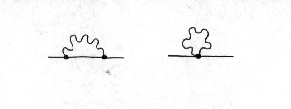
Figure 1: The fermion self-energy $\Sigma_{0}(x,y)$

Terms in which the fermion fields in the potential contract to each other do not occur.

The singularity comes from the non-summability of $\Sigma_{0}(x,y)$. As $d(x,y)\to\infty$ the best estimates uniform in $N$ are $(-\Delta+\mu_{0}^{2})^{-1}(xx^{\prime},yy^{\prime})={\cal O}(d(x,y)^{-1})$ for bosons and $(-D(0)+m_{0})^{-1}(x,y)={\cal O}(d(x,y)^{-2})$ for fermions and hence $\Sigma_{0}(x,y)={\cal O}(d(x,y)^{-3})$. This gives the logarithmic divergence when summed. The counterterm is chosen to compensate and we take

$$\delta m_{0}=-\sum_{y\in{\mathbb{T}}^{0}_{N+M}}\Sigma_{0}(x,y)$$ (18)

This is independent of $x$ by translation invariance.

When the cutoffs are removed the divergent part of $\delta m_{0}$ formally vanishes by symmetry considerations. This suggests that perhaps we do not really need the mass counterterm. We include it nevertheless as a convenient way to cancel dangerous looking terms in our effective actions. Along these lines we mention also that $\delta m_{0}$ is formally a Dirac scalar when the cutoffs are removed. We do not claim it is true as it stands.

The vacuum energy counterterm can also be chosen from looking at the divergences in perturbation theory. But now one would have to include all diagrams up to sixth order. We do not really want to go to the trouble of keeping track of all these diagrams, particularly since the vacuum energy does not contribute at all to the correlation functions. Instead we pick a counterterm by a method more suited to our analysis. The counterterm is taken to have the form

$$\delta E_{0}=\sum_{j=0}^{N-1}\delta{\cal E}_{j}\ L^{3(N+M-j)}$$ (19)

where the $j^{th}$ term is chosen to remove dangerous terms in the $(j+1)^{st}$ RG step. The factor $L^{3(N+M-j)}$ is the volume in which we will be working at that point. The energy densities $\delta{\cal E}_{j}$ are to be specified, but we will have $\delta{\cal E}_{j}={\cal O}(e_{j}^{2})$ where $e_{j}=L^{-(N-j)/2}$ is a running coupling constant. Note the quadratic divergence $\delta E_{0}={\cal O}(L^{2N})$.

2.3 the RG transformation

The renormalization group (RG) is a series of transformations which average out the short distance features of the model, leaving only the the long distance properties in which we are interested (now that we have scaled the model). Here we define a simple version of the first RG transformation. Our purpose is to explain the general idea and establish some notation. This simple version will not be suitable for iteration which is the eventual goal. Counterterms are omitted.

First we define averaging operators. These take functions on ${\mathbb{T}}_{N+M}^{0}$ to functions on ${\mathbb{T}}_{N+M}^{1}$ and are defined for spinors and vector fields respectively by

$$\begin{split}(Q_{e_{0}}(A)f)(y)&=L^{-3}\sum_{x\in B(y)}\exp\left(ie_{0}A(\Gamma_{yx})\right)f(x)\\ (Qh)_{\mu}(y)&=L^{-3}\sum_{x\in B(y)}h_{\mu}(x)\\ \end{split}$$ (20)

Here for $y\in{\mathbb{T}}_{N+M}^{1}$ we have defined

$$B(y)=\{x\in{\mathbb{T}}_{N+M}^{0}:|x-y|\leq L/2\}$$ (21)

The distance is $|x-y|=\sup_{\mu}|x_{\mu}-y_{\mu}|$ so this in an $L$-cube centered on $y$. We assume $L$ is odd so the $B(y)$ form a partition. Also $\Gamma_{yx}$ is a rectilinear path from $x$ to $y$ obtained by successively changing each of the three components, and $A(\Gamma)=\sum_{x^{\prime}x\in\Gamma}A_{x^{\prime}x}$. The spinor averaging operator is chosen to be gauge covariant:

$$Q_{e_{0}}(A-\partial\lambda)=e^{-ie_{0}\lambda}Q(A)e^{ie_{0}\lambda}$$ (22)

Let $Q_{e_{0}}(A)^{T},Q^{T}$ denote the transpose operators which take functions on ${\mathbb{T}}_{N+M}^{1}$ to functions on ${\mathbb{T}}_{N+M}^{0}$. These are defined with respect to the natural inner product on ${\mathbb{T}}_{N+M}^{1}$, i.e. sums are weighted by $L^{3}$. They are computed to be

$$\begin{split}(Q_{e_{0}}(A)^{T}f)(x)&=\exp\left(ie_{0}A(\Gamma_{yx})\right)f(y)\\ (Q^{T}h)_{\mu}(x)&=h_{\mu}(y)\\ \end{split}$$ (23)

where $y$ is the unique point so $x\in B(y)$. We have $Q_{e_{0}}(-A)Q_{e_{0}}(A)^{T}=I$ and $QQ^{T}=I$ while $Q_{e_{0}}(-A)^{T}Q_{e_{0}}(A)$ and $Q^{T}Q$ are projection operators.

Now starting with the density $\rho_{0}$ on ${\mathbb{T}}^{0}_{N+M}$ then we define a transformed density on ${\mathbb{T}}^{1}_{N+M}$ by

$$\begin{split}\tilde{\rho}_{1}(\Psi,A)=&c_{0}\int\exp\left(-\frac{a}{2L^{2}}|A-QA_{0}|^{2}\right)\exp\left(-\frac{a}{L}|\Psi-Q_{e_{0}}(A_{0})\Psi_{0}|^{2}\right)\\ &\rho_{0}(\Psi_{0},A_{0})\ d\Psi_{0}\ dA_{0}\\ \end{split}$$ (24)

We have passed to a larger Grassman algebra generated by $\Psi,\Psi_{0}$ and are now integrating over the $\Psi_{0}$ part of it. We have also introduced the (somewhat abusive) notation

$$|\Psi-Q(A_{0})\Psi_{0}|^{2}=(\bar{\Psi}-Q_{e_{0}}(-A_{0})\bar{\Psi}_{0},\Psi-Q_{e_{0}}(A_{0})\Psi_{0})$$ (25)

The positive constant $a$ is arbitrary and the constant $c_{0}$ is chosen so that

$$\int\tilde{\rho}_{1}(\Psi,A)\ d\Psi\ dA=\int\rho_{0}(\Psi_{0},A_{0})\ d\Psi_{0}\ dA_{0}$$ (26)

Now insert the expression for $\rho_{0}$ into (24). The quadratic form in $(A,A_{0})$ is

$$\frac{a}{2L^{2}}|A-QA_{0}|^{2}+\frac{1}{2}(A_{0},(-\Delta+\mu_{0}^{2})A_{0})$$ (27)

and we would like to diagonalize it. To this end we introduce

$$\Delta^{\#}\equiv-\Delta+\mu_{0}^{2}+\frac{a}{L^{2}}\ Q^{T}Q$$ (28)

This is positive and so we can also define

$$\begin{split}C=&(\Delta^{\#})^{-1}\\ H_{1}=&\frac{a}{L^{2}}\ (\Delta^{\#})^{-1}Q^{T}\\ \tilde{\Delta}_{1}=&\frac{a}{L^{2}}-\frac{a^{2}}{L^{4}}\ Q(\Delta^{\#})^{-1}Q^{T}\\ \end{split}$$ (29)

Here $C$ is an operator on ${\mathbb{T}}^{0}_{N+M}$ (more precisely an operator on functions on bonds in ${\mathbb{T}}^{0}_{N+M}$), $H_{1}$ is an operator from ${\mathbb{T}}^{1}_{N+M}$ to ${\mathbb{T}}^{0}_{N+M}$ , and $\tilde{\Delta}_{1}$ is an operator on ${\mathbb{T}}^{1}_{N+M}$. The quadratic form is diagonalized by the change of variables $A_{0}\to A_{0}+H_{1}A$. Under this transformation the quadratic form becomes

$$\frac{1}{2}(A,\tilde{\Delta}_{1}A)+\frac{1}{2}(A_{0},\Delta^{\#}A_{0})$$ (30)

We have split it into a piece for the background field $A$, and a piece for the fluctuation field $A_{0}$. Now identify the Gaussian measure

$$d\mu_{\stackrel{{\scriptstyle}}{{C_{0}}}}(A_{0})=Z_{1}^{-1}\exp\left(-\frac{1}{2}(A_{0},\Delta^{\#}A_{0})\right)dA_{0}$$ (31)

where $Z_{1}$ is a normalization factor. Defining $\tilde{A}=H_{1}A$, and omitting counterterms for simplicity our transformed density has become

$$\begin{split}&\tilde{\rho}_{1}(\Psi,A)=c_{0}\exp\left(-\frac{1}{2}(A,\tilde{\Delta}_{1}A)\right)\ Z_{1}\\ &\int\exp\left(-\frac{a}{L}|\Psi-Q_{e_{0}}(\tilde{A}+A_{0})\Psi_{0})|^{2}-(\bar{\Psi}_{0},(D_{e_{0}}(\tilde{A}+A_{0})+m_{0})\Psi_{0})\right)d\Psi_{0}\ d\mu_{C_{0}}(A_{0})\\ \end{split}$$ (32)

Next we define a potential $V_{0}$ by

$$\begin{split}&\frac{a}{L}|\Psi-Q_{e_{0}}(\tilde{A}+A_{0})\Psi_{0}|^{2}+(\bar{\Psi}_{0},(D_{e_{0}}(\tilde{A}+A_{0})+m_{0})\Psi_{0})\\ =&\frac{a}{L}|\Psi-Q_{e_{0}}(\tilde{A})\Psi_{0})|^{2}+(\bar{\Psi}_{0},(D_{e_{0}}(\tilde{A})+m_{0})\Psi_{0})+V_{0}(\Psi,\Psi_{0},\tilde{A},A_{0})\end{split}$$ (33)

Thus $V_{0}$ is the part of the fermion quadratic form depending on the fluctuation field $A_{0}$. The fluctuation field is massive due to the $Q^{T}Q$ in $\Delta^{\#}$. Hence large $A_{0}$ is suppressed and we can expect that $V_{0}$ is small. The most important contribution to $V_{0}$ is from the term

$$(\bar{\Psi}_{0},D_{e_{0}}(\tilde{A}+A_{0})\Psi_{0})-(\bar{\Psi}_{0},D_{e_{0}}(\tilde{A})\Psi_{0})=\sum_{xx^{\prime}}\bar{\Psi}_{0}(x)\gamma_{xx^{\prime}}e^{ie_{0}\tilde{A}(xx^{\prime})}(e^{ie_{0}A_{0}(xx^{\prime})}-1)\Psi_{0}(x^{\prime})$$ (34)

The lowest order term in $e_{0}$ gives the classical interaction vertex, but with the background $e^{ie_{0}\tilde{A}}$. Higher order terms give multiphoton vertices. There are also vertices coming from the $Q$ terms.

Now consider the fermion quadratic form with background field, i.e. the first two terms on the right side of (33). We want to diagonalize in $\Psi,\Psi_{0}$. This involves the inverse of the operator

$$D^{\#}(\tilde{A})\equiv D_{e_{0}}(\tilde{A})+m_{0}+\frac{a}{L}\ Q_{e_{0}}(-\tilde{A})^{T}Q_{e_{0}}(\tilde{A})$$ (35)

(We could write $Q_{e_{0}}(-\tilde{A})^{T}$ as $Q_{e_{0}}(\tilde{A})^{*}$ where the adjoint refers to a complex inner product). However we cannot control the inverse unless with have control over the field strength for $\tilde{A}$ . This is an issue we address in the the rest of the paper. For now we just assume that $e_{0}|\partial\tilde{A}|$ is sufficiently small. In this case we can define

$$\begin{split}\Gamma(\tilde{A})=&D^{\#}(\tilde{A})^{-1}\\ H_{1}(\tilde{A})=&\begin{cases}\frac{a}{L}\ D^{\#}(\tilde{A})^{-1}Q_{e_{0}}(-\tilde{A})^{T}&\textrm{ on }\Psi\\ \frac{a}{L}\ [D^{\#}(\tilde{A})^{-1}]^{T}Q_{e_{0}}(\tilde{A})^{T}&\textrm{ on }\bar{\Psi}\\ \end{cases}\\ \tilde{D}_{1}(\tilde{A})=&\ \frac{a}{L}-\frac{a^{2}}{L^{2}}\ Q_{e_{0}}(\tilde{A})D^{\#}(\tilde{A})^{-1}Q_{e_{0}}(-\tilde{A})^{T}\\ \end{split}$$ (36)

Now make the change of variables $\Psi_{0}\to\Psi_{0}+H_{1}(\tilde{A})\Psi$ and $\bar{\Psi}_{0}\to\bar{\Psi}_{0}+H_{1}(\tilde{A})\bar{\Psi}$. The quadratic form becomes

$$(\bar{\Psi},\tilde{D}_{1}(\tilde{A})\Psi)+(\bar{\Psi}_{0},D^{\#}(\tilde{A})\Psi_{0})$$ (37)

We identify the fermion Gaussian measure

$$d\mu_{\stackrel{{\scriptstyle}}{{\Gamma(\tilde{A})}}}(\Psi_{0})=\tilde{Z}_{1}(\tilde{A})^{-1}\exp\left(-(\bar{\Psi}_{0},D^{\#}(\tilde{A})\Psi_{0})\right)d\Psi_{0}$$ (38)

where $\tilde{Z}_{1}(\tilde{A})$ is the normalization factor. With $\tilde{\Psi}(\tilde{A})=H_{1}(\tilde{A})\Psi$ the complete fluctuation integral is now the Gaussian integral

$$\tilde{\Xi}_{1}(\Psi,\tilde{A})\equiv\int\exp\left(-V_{0}(\Psi,\Psi_{0}+\tilde{\Psi}(\tilde{A}),\tilde{A},A_{0})\right)d\mu_{\stackrel{{\scriptstyle}}{{\Gamma(\tilde{A})}}}(\Psi_{0})d\mu_{\stackrel{{\scriptstyle}}{{C}}}(A_{0})$$ (39)

and the overall density is

$$\tilde{\rho}_{1}(\Psi,A)=c_{0}\exp\left(-\frac{1}{2}(A,\tilde{\Delta}_{1}A))-(\bar{\Psi},\tilde{D}_{1}(\tilde{A})\Psi)\right)Z_{1}\tilde{Z}_{1}(\tilde{A})\ \tilde{\Xi}_{1}(\Psi,\tilde{A})$$ (40)

We note that $(\bar{\Psi},\tilde{D}_{1}(\tilde{A})\Psi)$ and $\tilde{Z}_{1}(\tilde{A})$ and $\tilde{\Xi}_{1}(\Psi,\tilde{A})$ are all invariant under gauge transformations in the variables $(\bar{\Psi},\Psi,\tilde{A})$. (They would not be invariant in the fundamental variables $(\bar{\Psi},\Psi,A$).)

Finally we scale back to fields on a unit lattice. For $\Psi_{1},A_{1}$ on ${\mathbb{T}}^{0}_{N+M-1}$ by we define

$$\rho_{1}(\Psi_{1},A_{1})=\tilde{\rho}_{1}(\Psi_{1,L},A_{1,L})$$ (41)

For the boson parts of this we define ${\cal Q}=\sigma_{L}^{-1}Q\sigma_{L}$ which is the natural averaging operator mapping functions on ${\mathbb{T}}^{-1}_{N+M-1}$ (an $L^{-1}$ lattice ) to functions on ${\mathbb{T}}^{0}_{N+M-1}$. Then we define

$$\begin{split}G_{1}=&L^{-2}\sigma_{L}^{-1}C_{0}\ \sigma_{L}=\left(-\Delta+\mu_{1}^{2}+{\cal Q}^{T}{\cal Q}\right)^{-1}\\ {\cal H}_{1}=&\sigma_{L}^{-1}H_{1}\sigma_{L}=a\ G_{1}{\cal Q}^{T}\\ \Delta_{1}=&L^{2}\sigma_{L}^{-1}\tilde{\Delta}_{1}\sigma_{L}=aI-a^{2}{\cal Q}G_{1}{\cal Q}^{T}\\ \end{split}$$ (42)

Here $G_{1}$ is on operator on on ${\mathbb{T}}^{-1}_{N+M-1}$ , ${\cal H}_{1}$ is an operator from ${\mathbb{T}}^{0}_{N+M-1}$ to ${\mathbb{T}}^{-1}_{N+M-1}$, and $\Delta_{1}$ is an operator on ${\mathbb{T}}^{0}_{N+M-1}$. The background field $\tilde{A}=H_{1}A$ scales to $H_{1}A_{1,L}$ on ${\mathbb{T}}^{0}_{N+M}$, and it can now be written ${\cal A}_{1,L}$ where ${\cal A}_{1}={\cal H}_{1}A_{1}$ is a field on ${\mathbb{T}}^{-1}_{N+M-1}$

Now for fermions we define ${\cal Q}_{e_{1}}({\cal A}_{1})=\sigma_{L}^{-1}Q_{e_{0}}({\cal A}_{1,L})\sigma_{L}$ which is the natural averaging operator on ${\mathbb{T}}^{-1}_{N+M-1}$ with $e_{1},{\cal A}_{1}$. Then we define

$$\begin{split}S_{1}({\cal A}_{1})=&L^{-1}\sigma_{L}^{-1}\Gamma_{0}({\cal A}_{1,L})\ \sigma_{L}=\left(D_{e_{1}}({\cal A}_{1})+m_{1}+{\cal Q}_{e_{1}}(-{\cal A}_{1})^{T}{\cal Q}_{e_{1}}({\cal A}_{1})\right)^{-1}\\ {\cal H}_{1}({\cal A}_{1})=&\sigma_{L}^{-1}H_{1}({\cal A}_{1,L})\sigma_{L}=\begin{cases}aS_{1}({\cal A}_{1}){\cal Q}_{e_{1}}(-{\cal A}_{1})^{T}&\textrm{ on }\Psi\\ aS_{1}({\cal A}_{1})^{T}{\cal Q}_{e_{1}}({\cal A}_{1})^{T}&\textrm{ on }\bar{\Psi}\\ \end{cases}\\ D_{1}({\cal A}_{1})=&L\ \sigma_{L}^{-1}\tilde{D}_{1}({\cal A}_{1,L})\sigma_{L}=aI-a^{2}{\cal Q}_{e_{1}}({\cal A}_{1})S_{1}({\cal A}_{1}){\cal Q}_{e_{1}}(-{\cal A}_{1})^{T}\\ \end{split}$$ (43)

The fermi field $\tilde{\Psi}(\tilde{A})$ scales to $H_{1}({\cal A}_{1,L})\Psi_{1,L}$ which can be written $(\psi_{1}({\cal A}_{1}))_{L}$ where $\psi_{1}({\cal A}_{1})\equiv{\cal H}_{1}({\cal A}_{1})\Psi_{1}$. This field appears in the scaled fluctuation integral

$$\Xi_{1}(\Psi_{1},{\cal A}_{1})=\tilde{\Xi}_{1}(\Psi_{1,L},{\cal A}_{1,L})$$ (44)

We also define $Z_{1}({\cal A}_{1})=\tilde{Z}_{1}({\cal A}_{1,L})$. Then we have for the new density (still under a small field assumption)

$$\rho_{1}(\Psi_{1},A_{1})=c_{0}\exp\left(-\frac{1}{2}(A_{1},\Delta_{1}A_{1}))-(\bar{\Psi}_{1},D_{1}({\cal A}_{1})\Psi_{1})\right)Z_{1}Z_{1}({\cal A}_{1})\Xi_{1}(\Psi_{1},{\cal A}_{1})$$ (45)

This expression shows a nice split into a kinetic part (the exponential) and an effective interaction (the rest). Next one could compute the leading contributions to $Z_{1}({\cal A}_{1})$ and $\Xi_{1}(\Psi_{1},{\cal A}_{1})$ in perturbation theory. However we leave this for the full treatment.

Another representation: Suppose we undo some of the steps that got us here. Go back to the expression (40) for $\tilde{\rho}_{1}(\Psi,A)$. Express $\tilde{Z}_{1}(\tilde{A})$ and $Z_{1}$ as integrals over $\Psi_{0}$ and $A_{0}$ and then make the inverse transformations $\Psi_{0}\to\Psi_{0}-\tilde{\Psi}(\tilde{A})$ and $A_{0}\to A_{0}-\tilde{A}$. This yields

$$\begin{split}\tilde{\rho}_{1}(\Psi,A)=&c_{0}\ \tilde{\Xi}_{1}(\Psi,\tilde{A})\int\exp\left(-\frac{a}{2L^{2}}|A-QA_{0}|^{2}\right)\exp\left(-\frac{a}{L}|\Psi-Q(\tilde{A})\Psi_{0}|^{2}\right)\\ &\exp\left(-\frac{1}{2}(A_{0},(-\Delta+\mu_{0}^{2})A_{0})-(\bar{\Psi}_{0},(D_{e_{0}}(\tilde{A})+m_{0})\Psi_{0})\right)d\Psi_{0}\ dA_{0}\\ \end{split}$$ (46)

This can also be scaled to get another representation for $\rho_{1}(\Psi_{1},A_{1})$. The expression (46) is close to what we started with in (24). The change is that the gauge field $A_{0}$ has been replaced with a background field $\tilde{A}$ with fewer degrees of freedom, and there is a corresponding correction factor $\tilde{\Xi}_{1}(\Psi,\tilde{A})$. Variations of this representation will be useful for iteration.

2.4 some tools

We introduce some tools that we need for subsequent developments. These are roughly ordered by length scale.

A. We use random walk expansions for the basic propagators $C$ and $\Gamma(A)$ assuming $e_{0}|\partial A|$ is sufficiently small. These are developed on a scale $M_{0}$ which is a fixed power of $L$. We consider the $M_{0}$ lattice ${\mathbb{T}}^{M_{0}}_{N+M}$ A path is a sequence $\omega=(j_{0},j_{1},\dots,j_{n})$ of points in this lattice which are neighbors in the sense that $|j_{\alpha}-j_{\alpha+1}|=0\textrm{ or }M_{0}$. Associated with a path $\omega$ is a sequence $({\cal O}_{j_{0}},{\cal O}_{j_{1}},\cdots,{\cal O}_{j_{n}})$ of overlapping $2M_{0}$ cubes ${\cal O}_{j}$ centered on the points $j$. We write $\omega:x\to y$ if $x\in{\cal O}_{j_{0}}$ and $y\in{\cal O}_{j_{n}}$.

The random walk expansion has the form

$$\begin{split}\Gamma(A,x,y)=&\sum_{\omega:x\to y}\Gamma_{\omega}(A,x,y)\\ C(x,y)=&\sum_{\omega:x\to y}C_{\omega}(x,y)\\ \end{split}$$ (47)

The individual terms are $({\cal O}(1)M_{0}^{-1})^{\ell(\omega)}$ where $\ell(\omega)$=number of steps in $\omega$, and this is sufficient for convergence if $M_{0}$ is large enough. From the condition $\omega:x\to y$ we can also extract some exponential decay and obtain for $\beta={\cal O}(M_{0}^{-1})$

$$|\Gamma(A,x,y)|,\ \ |C(x,y)|\leq C\exp(-\beta d(x,y))$$ (48)

We also note that $\Gamma_{\Lambda,\omega}(A)$ depends on $A$ only in ${\cal O}_{j_{0}}\cup{\cal O}_{j_{1}}\cup\cdots\cup{\cal O}_{j_{n}}$.

See appendix A for details of this construction and the original references.

B. The fluctuation integrals will be processed by a cluster expansion. This means all terms must be localized. This will be done on a scale $M_{1}$, also a fixed power of $L$ but larger than $M_{0}$. $\Delta$ will denote a $M_{1}$ cube centered on the ${\mathbb{T}}^{M_{1}}_{N+M}$ lattice. These partition the lattice. A union of such $\Delta$ will be denoted by $X,Y,Z,\dots$. Such a set is connected and called a polymer if for any two $\Delta,\Delta^{\prime}\subset X$ there is a sequence $\Delta,\Delta_{1},\dots\Delta_{n},\Delta^{\prime}$ in $X$ such that consecutive blocks touch in any dimension. The terms in our effective potentials will be polymer sums $\sum_{X}E(X)$ where $E(X)$ only depends on fields in $X$.

C. We introduce a scale beyond which correlations are completely negligible. This is defined by

$$r(e_{0})=(\log e_{0}^{-1})^{r}=\left(\frac{N}{2}+\log e^{-1}\right)^{r}$$ (49)

for some small positive integer $r$. If $N$ is large then $e_{0}$ is small and $r(e_{0})$ is large; we assume it is larger than $M_{1}$. Let $R_{0}=\inf_{m}\{L^{m}:L^{m}\geq r(e_{0})\}$ be an associated power of $L$. We will consider blocks $\square$ of size $R_{0}$ centered on points in ${\mathbb{T}}^{R_{0}}_{N+M}$ and collections of such blocks denoted $\Omega,\Lambda,...$.

We also will use approximate propagators which do not couple beyond this scale. These are defined in terms of the random walk expansion. Let $\chi_{\omega}(x,y)$ is the characteristic function of paths which stay within $r(e_{0})/2$ of both $x$ and $y$. Then we define

$$\begin{split}C^{loc}(x,y)=&\sum_{\omega:x\to y}C_{\omega}(x,y)\chi_{\omega}(x,y)\\ \Gamma^{loc}(A,x,y)=&\sum_{\omega:x\to y}\Gamma_{\omega}(A,x,y)\chi_{\omega}(x,y)\\ \end{split}$$ (50)

These vanish for $d(x,y)\geq r(e_{0})/2$ and still satisfy (48).

D. We introduce a scale which distinguishes between large and small values of $|\partial A|$. This is defined by

$$p(e_{0})=(\log e_{0}^{-1})^{p}=\left(\frac{N}{2}+\log e^{-1}\right)^{p}$$ (51)

for some integer $p$ larger than $r$. “Small fields” will satisfy conditions like $|\partial A|\leq{\cal O}(p(e_{0}))$ and may actually be rather large. Still $e_{0}|\partial A|$ would be small as required for the existence of $\Gamma(A)$.

F. Finally we discuss introduce some norms for fermions. Let $\xi$ stand for $(0,\alpha,x)$ or $(1,\alpha,x)$ with $x\in{\mathbb{T}}^{0}_{N+M}$ and $1\leq\alpha\leq 4$. Then define $\Psi(0,\alpha,x)=\Psi_{\alpha}(x)$ and $\Psi(1,\alpha,x)=\bar{\Psi}_{\alpha}(x)$. We consider elements of the Grassmann algebra of the form:

$$K(\Psi)=\sum_{n=0}^{\infty}1/n!\sum_{\xi_{1},...,\xi_{n}}k_{n}(\xi_{1},...,\xi_{n})\Psi(\xi_{1})...\Psi(\xi_{n})$$ (52)

The kernel $k_{n}$ may also depend on the gauge field $A$. A family of norms is defined by

$$\|K\|_{h}=\sum_{n=0}^{\infty}\frac{h^{n}}{n!}\|k_{n}\|_{1}$$ (53)

where $\|k_{n}\|_{1}$ is the $\ell_{1}$ norm and $h={\cal O}(1)$ is an adjustable parameter. These norms satisfy $\|KL\|_{h}\leq\|K\|_{h}\|L\|_{h}$. Properties and variations are discussed in appendix B.

We will also want to consider functions which only depend on dressed fields like $\tilde{\Psi}=\tilde{\Psi}(\tilde{A})=H_{1}(\tilde{A})\Psi$. These would have the form

$$K(\tilde{\Psi})=\sum_{n=0}^{\infty}1/n!\sum_{\xi_{1},...,\xi_{n}}k_{n}(\xi_{1},...,\xi_{n})\tilde{\Psi}(\xi_{1})...\tilde{\Psi}(\xi_{n})$$ (54)

We define a kernel norm by

$$|K|_{h}=\sum_{n=0}^{\infty}\frac{h^{n}}{n!}\|k_{n}\|_{1}$$ (55)

This still satisfies $|KL|_{h}\leq|K|_{h}|L|_{h}$.

3 The first step

We now give another version of the first RG transformation and this time it is something we can iterate. The idea is to break up the RG integral over the gauge field into a large fields and small fields. This is done at each point in space time we generate a sum over regions where the field is large and regions where the field is small. In the small field region we can carry out the analysis of effective action that we have sketched. Furthermore we can make a perturbation expansion with good control over the remainder. The contribution of the large field region makes a tiny contribution due to tiny factors from the free action. These small factors are enough to control the sum over the regions. We now enter into the details which follow especially [2], [8].

3.1 the split

We analyze (24), but now splitting into large and small field regions. The small field region will be a set on which the following inequalities hold

$$\begin{split}|\partial A_{0}|\leq&\ \ p(e_{0})\\ |A_{0}|\leq&\ \ \mu_{0}^{-1}p(e_{0})\\ |A-QA_{0}|\leq&\ \ p(e_{0})\\ \end{split}$$ (56)

These correspond to various terms in the action. Fields which violate them will be exponentially suppressed.

Specifically we insert under the integral sign the expression

$$1=\sum_{\Omega}\zeta_{0}(\Omega^{c},A,A_{0})\chi_{0}(\Omega,A,A_{0})$$ (57)

Here $\Omega$ is an arbitrary collection of blocks $\square$ of size $R_{0}$. The function $\chi_{0}(\Omega,A,A_{0})$ enforces the inequalities (56) on $\Omega$ and we take it to have the form

$$\begin{split}&\chi_{0}(\Omega,A,A_{0})\\ =&\prod_{x\in\Omega}\chi(|\partial A_{0}(x)|/p(e_{0}))\prod_{x\in\Omega}\chi(|A_{0}(x)|/\mu_{0}^{-1}p(e_{0}))\prod_{y\in\Omega}\chi(|(A-QA_{0})(y)|/p(e_{0}))\\ \end{split}$$ (58)

where $\chi(\alpha)$ is a smooth positive function interpolating between $\chi=1$ for $|\alpha|\leq\frac{1}{2}$ and $\chi=0$ for $|\alpha|\geq 1$. We assume the derivatives satisfy $|\chi^{(n)}|\leq{\cal O}(n!^{2})$. The function $\zeta_{0}(\Omega^{c},A,A_{0})$ is also smooth and enforces that at least one of the inequalities (56) (with a factor $\frac{1}{2}$) is violated at some point in every block in $\Omega^{c}$. For the explicit formula see [2], [8].

Now we have

$$\begin{split}&\tilde{\rho}_{1}(\Psi,A)=c_{0}e^{\delta E_{0}}\sum_{\Omega}\int d\Psi_{0}dA_{0}\ \zeta_{0}(\Omega^{c},A,A_{0})\ \chi_{0}(\Omega,A,A_{0})\\ &\exp\left(-\frac{a}{2L^{2}}|A-QA_{0}|^{2}-\frac{1}{2}(A_{0},(-\Delta+\mu_{0}^{2})A_{0})\right)\\ &\exp\left(-\frac{a}{L}|\Psi-Q_{e_{0}}(A_{0})\Psi_{0}|^{2}+(\bar{\Psi}_{0},(D_{e_{0}}(A_{0})+m_{0})\Psi_{0})-v(\delta m_{0})\right)\ \\ \end{split}$$ (59)

3.2 boson translation

Again we seek to diagonalize the boson quadratic form, but now only in the small field region. We define a local version of $H_{1}$ by

$$H_{1}^{loc}=\frac{a}{L^{2}}C^{loc}Q^{T}$$ (60)

We approximately diagonalize by making the transformation

$$A_{0}\to A_{0}+[H_{1}^{loc}A]_{\Omega^{\prime}}\equiv A_{0}+\tilde{A}_{\Omega^{\prime}}$$ (61)

Here $\Omega^{\prime}$ is $\Omega$ shrunk by a corridor of $R_{0}$ blocks so that $d(\Omega^{c},\Omega^{\prime})=R_{0}\geq r(e_{0})$. Since $H_{1}^{loc}$ has range $r(e_{0})/2$ the expression $[H_{1}^{loc}A]_{\Omega^{\prime}}$ only depends on $A$ in $\Omega$ where we have some control.

Lemma 1

Under the transformation (61) the boson quadratic form (27) becomes

$$\frac{1}{2}(A,[\tilde{\Delta}_{1}]_{\Omega}A)+\frac{1}{2}(A_{0},\Delta^{\#}A_{0})+F^{b}+W^{b}$$ (62)

Here each $F^{b}=F^{b}(A,A_{0})$ is localized in $(\Omega^{\prime\prime})^{c}$ and $W^{b}=W^{b}(A,A_{0})$ has the form $W^{b}=\sum_{X\subset\Omega}W^{b}(X)$ where the sum is over polymers $X$. The function $W^{b}(X)=W^{b}(X,A,A_{0})$ only depends on $A,A_{0}$ in $X$. Assuming the bounds (56) we have with $\beta=M_{0}^{-1}$

$$|W^{b}(X,A,A_{0})|\leq{\cal O}(1)e^{-\frac{1}{2}\beta r(e_{0})}e^{-\frac{1}{2}\beta M_{1}|X|_{1}}$$ (63)

Remarks. Here are some notational conventions

1. If $f$ is a function then $f_{\Omega}=\chi_{\Omega}f$ is the restriction to $\Omega$. If $T$ is an operator the $T_{\Omega}=\chi_{\Omega}T\chi_{\Omega}$ and $T_{\Omega\Omega^{\prime}}=\chi_{\Omega}T\chi_{\Omega^{\prime}}$.

2. The general convention is that constants denoted ${\cal O}(1)$ may depend on the parameters $L,M_{0},M_{1},\mu$, but not on $e,m$ or on the fundamental cutoffs $N,M$. A constant which is independent of all parameters is designated as universal.

3. The symbol $|X|_{1}$ stands for the number of elementary $M_{1}$ blocks in $X$. Thus the volume is $|X|=M_{1}^{3}|X|_{1}$. The quantity $M_{1}|X|_{1}$ is the linear size of $|X|$. In fact if ${\cal L}(X)$ is the length of the shortest tree joining the centers of the blocks in $X$ then ${\cal L}(X)=M_{1}(|X|_{1}-1)$. We could have written the bound with ${\cal L}(X)$. Since $\beta M_{1}={\cal O}(M_{0}^{-1}M_{1})$ is assumed large the factor $e^{-\frac{1}{2}\beta M_{1}|X|_{1}}$ controls the sum over $X$. The relevant standard bound is that for $\kappa$ large enough

   $$\sum_{X\supset\Delta}e^{-\kappa|X|_{1}}\leq 1$$ (64)

   Or we could replace the condition $X\supset\Delta$ by $X$ touches $\Delta$.

4. Note that $e^{-r(e_{0})}={\cal O}(e_{0}^{n})$ for any $n$; it is extremely small.

Proof. Making the translation the term quadratic in $A_{0}$ remains $\frac{1}{2}(A_{0},\Delta^{\#}A_{0})$ where $\Delta^{\#}$ is defined in ( 28).

The cross term is

$$(A_{0},\Delta^{\#}[H_{1}^{loc}A]_{\Omega^{\prime}})-\frac{a}{L^{2}}(QA_{0},A)$$ (65)

We replace $A_{0}$ by $A_{0,\Omega}$. In the first term there is no change and the difference for the second term is localized in $\Omega^{c}$ and contributes to $F^{b}$. Thus it suffices to consider (65) with $A_{0,\Omega}$. Next we write

$$[H_{1}^{loc}A]_{\Omega^{\prime}}=[H_{1}^{loc}A_{\Omega}]_{\Omega^{\prime}}=H_{1}^{loc}A_{\Omega}-[H_{1}^{loc}A_{\Omega}]_{(\Omega^{\prime})^{c}}$$ (66)

The term $[H_{1}^{loc}A_{\Omega}]_{(\Omega^{\prime})^{c}}$ has $A$ dependence in $\Omega\cap(\Omega^{\prime\prime})^{c}$, and its contribution also has $A_{0}$ dependence in this set. Thus these terms contribute to $F^{b}$. We are left with

$$(A_{0,\Omega},\Delta^{\#}H_{1}^{loc}A_{\Omega})-\frac{a}{L^{2}}(QA_{0,\Omega},A_{\Omega})$$ (67)

If we replace $H_{1}^{loc}$ by $H_{1}$ we get zero. Thus we can write this term as

$$W_{1}\equiv(A_{0,\Omega},\Delta^{\#}(H_{1}^{loc}-H_{1})A_{\Omega})$$ (68)

The terms quadratic in $A$ have the form

$$\frac{a}{2L^{2}}(A,A)-\frac{a}{L^{2}}(A,Q[H_{1}^{loc}A]_{\Omega^{\prime}})+\frac{1}{2}([H_{1}^{loc}A]_{\Omega^{\prime}},\Delta^{\#}[H_{1}^{loc}A]_{\Omega^{\prime}})$$ (69)

We replace $A$ by $A_{\Omega}$. The difference only comes from the first term and it contributes to $F^{b}$. We also insert (66) and again the terms arising from $[H_{1}^{loc}A_{\Omega}]_{(\Omega^{\prime})^{c}}$ are all localized in $\Omega\cap(\Omega^{\prime\prime})^{c}$ and contribute to $F_{b}$. We are left with

$$\frac{a}{2L^{2}}(A_{\Omega},A_{\Omega})-\frac{a}{L^{2}}(A_{\Omega},QH_{1}^{loc}A_{\Omega})+\frac{1}{2}(H_{1}^{loc}A_{\Omega},\Delta^{\#}H_{1}^{loc}A_{\Omega})$$ (70)

If we replace $H_{1}^{loc}$ by $H_{1}$ we get $\frac{1}{2}(A_{\Omega},\tilde{\Delta}_{1}A_{\Omega})=\frac{1}{2}(A,\tilde{\Delta}_{1,\Omega}A)$. The difference is

$$\begin{split}W_{2}\equiv&-\frac{a}{L^{2}}(A_{\Omega},Q(H_{1}^{loc}-H_{1})A_{\Omega})\\ &+\frac{1}{2}((H^{loc}_{1}-H_{1})A_{\Omega},\Delta^{\#}H_{1}^{loc}A_{\Omega})+\frac{1}{2}(H_{1}A_{\Omega},\Delta^{\#}(H_{1}^{loc}-H_{1})A_{\Omega})\\ \end{split}$$ (71)

Now we have established the representation (62) with $W^{b}=W_{1}+W_{2}$.

Let us analyze $W_{1}$. It can be written

$$W_{1}=(A_{0},w_{1}A)=\sum_{x,y\in\Omega}A_{\mu,0}(x)w_{1,\mu,\nu}(x,y)A_{\nu}(y)$$ (72)

Now $w_{1}$ depends on $H_{1}-H_{1}^{loc}$ and hence on $C-C^{loc}$. In appendix A, lemma 17, we use a random walk expansion to find a local expansion $C-C^{loc}=\sum_{X}\delta C(X)$ in which $\delta C_{\mu,\nu}(X,x,y)$ is supported on $X\times X$ and only very large $X$ contribute. This leads to an expansion $w_{1}=\sum_{X}w_{1}(X)$ with $w_{1,\mu,\nu}(X,x,y)$ supported on $X\times X$ and satisfying

$$|w_{1}(X,x,y)|\leq{\cal O}(1)e^{-\beta r(e_{0})}e^{-\beta M_{1}|X|_{1}}e^{-\beta d(x,y)}$$ (73)

Now we have $W_{1}=\sum_{X}W_{1}(X)$ where $W_{1}(X)=(A_{0},w_{1}(X)A)$. We have the weak bounds $|A_{0}|\leq\mu_{0}^{-1}p(e_{0})$ and

$$|A|\leq|A-QA_{0}|+|QA_{0}|\leq{\cal O}(\mu_{0}^{-1}p(e_{0}))$$ (74)

The factors ${\cal O}(\mu_{0}^{-1}p(e_{0}))$ are compensated by a factor $e^{-\frac{1}{2}\beta r(e_{0})}$. We also get a volume factor $|X|=M_{1}^{3}|X|_{1}$ which is dominated by a factor $e^{-\frac{1}{2}\beta M_{1}|X|_{1}}$. Overall we have

$$|W_{1}(X)|\leq e^{-\frac{1}{2}\beta r(e_{0})}e^{-\frac{1}{2}\beta M_{1}|X|_{1}}$$ (75)

The analysis of $W_{2}$ is similar. This completes the proof.

At this point we have

$$\begin{split}&\tilde{\rho}_{1}(\Psi,A)=c_{0}e^{\delta E_{0}}\sum_{\Omega}\int d\Psi_{0}dA_{0}\ \zeta_{0}(\Omega^{c},A,A_{0})\ \chi_{0}(\Omega,A,\tilde{A}_{\Omega^{\prime}}+A_{0})\\ &\exp\left(-\frac{1}{2}(A,\tilde{\Delta}_{1,\Omega}A)-\frac{1}{2}(A_{0},\Delta^{\#}A_{0})-F^{b}-W^{b})\right)\\ &\exp\left(-\frac{a}{L}|\Psi-Q_{e_{0}}(\tilde{A}_{\Omega^{\prime}}+A_{0})\Psi_{0}|^{2}-(\bar{\Psi}_{0},(D_{e_{0}}(\tilde{A}_{\Omega^{\prime}}+A_{0})+m_{0})\Psi_{0})-v(\delta m_{0})\right)\ \\ \end{split}$$ (76)

3.3 new field restrictions

Let us consider the characteristic function $\chi_{0}(\Omega,A,\tilde{A}_{\Omega^{\prime}}+A_{0})$ where we recall that $A$ is a function on ${\mathbb{T}}^{1}_{N+M}$ and that $A_{0},\tilde{A}=H_{1}^{loc}A$ are functions on ${\mathbb{T}}^{0}_{N+M}$. The characteristic function imposes that on $\Omega^{\prime}$

$$\begin{split}|\partial(\tilde{A}+A_{0})|\leq&\ \ p(e_{0})\\ |\tilde{A}+A_{0}|\leq&\ \ \mu_{0}^{-1}p(e_{0})\\ |A-Q(\tilde{A}+A_{0})|\leq&\ \ p(e_{0})\\ \end{split}$$ (77)

These inequalities imply inequalities on the fields $A,A_{0},\tilde{A}$ separately as follows

Lemma 2

Assume, (77) holds on $\Omega^{\prime}$. Then there are constants $C_{1},C_{2}$ such that

1. $|\partial A|\leq C_{1}p(e_{0})$ and $|A|\leq C_{1}\mu_{0}^{-1}p(e_{0})$ on $\Omega^{\prime}$.

2. $\tilde{A}=Q^{T}A+{\cal O}(p(e_{0}))$ on $\Omega^{\prime\prime}$

3. $|A_{0}|\leq\ \ C_{1}p(e_{0})$ on $\Omega^{\prime\prime}$

4. $|\partial\tilde{A}|\leq C_{2}p(e_{0})$ and $|\tilde{A}|\leq C_{2}\mu_{0}^{-1}p(e_{0})$ on $\Omega^{\prime\prime}$

Remarks. The bound ${\cal O}(p(e_{0}))$ on the fluctuation field $A_{0}$ is a substantial improvement over ${\cal O}(\mu_{0}^{-1}p(e_{0}))$. Since we are on a unit lattice we have the same bound for $\partial A_{0}$.

The last bound follows directly from (1.) and (3.), a fact we use later on.

Proof. The proof follows [2].

1. Let $\check{A}=\tilde{A}+A_{0}$. We have for $y,y+Le_{\mu}\in\Omega^{\prime}$

   $$\begin{split}|(\partial_{\mu}A_{\nu})(y)|=&L|A_{\nu}(y)-A_{\nu}(y+Le_{\mu})|\\ \leq&L|(Q\check{A}_{\nu})(y)-(Q\check{A}_{\nu})(y+Le_{\mu})|+{\cal O}(p(e_{0}))\\ \leq&{\cal O}(p(e_{0}))\end{split}$$ (78)

   where we have used the first and third bounds in (77) . This proves the bound on $\partial A$. The bound on $|A|$ follows similarly from second and third bounds in (77).

2. If $x\in B(y)$ then $(Q^{T}A)(x)=A(y)$. Thus we must show that for $x\in B(y)\subset\Omega^{\prime\prime}$ that

   $$\tilde{A}(x)=A(y)+{\cal O}(p(e_{0}))$$ (79)

   We write

   $$\tilde{A}(x)=(H_{1}^{loc}A_{\Omega^{\prime}})(x)=\left(H^{loc}_{1}1_{\Omega^{\prime}})(x)A(y)+(H^{loc}_{1}(A_{\Omega^{\prime}}-1_{\Omega^{\prime}}A(y))\right)(x)$$ (80)

   The second term in (80) is $\sum_{y^{\prime}\in\Omega^{\prime}}H^{loc}_{1}(x,y)(A(y^{\prime})-A(y))$. This vanishes unless $x$ and hence $y$ are in the same component of $\Omega^{\prime}$ as $y^{\prime}$. Thus we can use the estimate on $\partial A$ to get $|A(y^{\prime})-A(y)|\leq d(y,y^{\prime}){\cal O}(p(e_{0}))$. The term is then ${\cal O}(p(e_{0}))$.

   For the first term in (80) we write

   $$(H^{loc}_{1}1_{\Omega^{\prime}})(x)=(H_{1}1)(x)-(H_{1}1_{(\Omega^{\prime})^{c}})(x)+((H^{loc}_{1}-H_{1})1_{\Omega^{\prime}})(x)$$ (81)

   For the last term here we again use lemma 17 which has tiny factors $e^{-r(e_{0})}$ to dominate the ${\cal O}(\mu_{0}^{-1}p(e_{0}))$ bound on $A(y)$ and give ${\cal O}(p(e_{0}))$ (or better). For the second term $H_{1}$ connects $x\in\Omega^{\prime\prime}$ to points in $(\Omega^{\prime})^{c}$ and thus also has tiny factors from the decay of $H_{1}$. For the first term we have

   $$\begin{split}H_{1}1=&\frac{a}{L^{2}}CQ^{T}1=C(\frac{a}{L^{2}}Q^{T}Q)1\\ =&1-C(-\Delta_{\Omega}+\mu_{0}^{2})1=1+{\cal O}(\mu_{0}^{2})\\ \end{split}$$ (82)

   Hence $(H_{1}1)(x)A(y)=A(y)+{\cal O}(p(e_{0}))$ and hence the result.

3. Now consider the bound on $A_{0}=\check{A}-\tilde{A}$. For $x\in B(y)\subset\Omega^{\prime\prime}$ we have

   $$|A_{0}(x)|\leq|\check{A}(x)-(Q\check{A})(y)|+|(Q\check{A})(y)-A(y)|+|A(y)-\tilde{A}(x)|$$ (83)

   The first term is ${\cal O}(p(e_{0}))$ by the first bound in (77), and the second term is ${\cal O}(p(e_{0})$ by the third bound in (77). For the last term we use (79 ).

4. This follows using the bounds (77) and the bounds on $A_{0}$. But we want to also show that it follows just from (1.) and (3.). In fact if (1.) holds then the identity (79) holds. Hence the bound on $\tilde{A}$ follows from the bound on $A$ and the bound on $\partial\tilde{A}$ follows from the bound on $\partial A$. In the latter case look at $(\partial_{\mu}\tilde{A}_{\nu})(x)=\tilde{A}(x+e_{\mu})-\tilde{A}(x)$ separately in the cases where $x$ and $x+e_{\mu}$ are or are not in the same $B(y)$. This completes the proof.

Now introduce new characteristic functions enforcing the conditions on $A,A_{0}$ by defining

$$\begin{split}\tilde{\chi}_{1}(\Omega^{\prime\prime},A)=&\prod_{x\in\Omega^{\prime\prime}}\chi\left(\frac{|\partial A(x)|}{2C_{1}p(e_{0})}\right)\prod_{x\in\Omega^{\prime\prime}}\chi\left(\frac{|A(x)|}{2C_{1}\mu_{0}^{-1}p(e_{0})}\right)\\ \chi^{*}(\Omega^{\prime\prime},A_{0})=&\prod_{x\in\Omega^{\prime\prime}}\chi\left(\frac{|A_{0}(x)|}{2C_{1}p(e_{0})}\right)\\ \end{split}$$ (84)

and inserting $\tilde{\chi}_{1}(\Omega^{\prime\prime},A)\chi^{*}(\Omega^{\prime\prime},A_{0})$ under the integral sign in (76).

Consider the old factor

$$\chi_{0}(\Omega,A,\tilde{A}_{\Omega^{\prime}}+A_{0})=\chi_{0}(\Omega-\Omega^{\prime\prime},A,\tilde{A}_{\Omega^{\prime}}+A_{0})\chi_{0}(\Omega^{\prime\prime},A,\tilde{A}+A_{0})$$ (85)

With the new characteristic functions in place it is safe to break up the second factor by replacing $\chi$ by $1+(1-\chi)$ at each point. We get an expansion of the form

$$\chi_{0}(\Omega^{\prime\prime},A,\tilde{A}+A_{0})=\sum_{\tilde{\Lambda}\subset\Omega^{\prime\prime}}\bar{\zeta}(\Omega^{\prime\prime}-\tilde{\Lambda},A,\tilde{A}+A_{0})$$ (86)

The sum is over unions of $R_{0}$ blocks $\tilde{\Lambda}\subset\Omega^{\prime\prime}$ and the function $\zeta(\Omega^{\prime\prime}-\tilde{\Lambda},A,\tilde{A}+A_{0})$ forces at least one of the inequalities (77) to be violated in each block in $\Omega^{\prime\prime}-\tilde{\Lambda}$.

Let us collect some of the the characteristic functions into

$$\begin{split}\chi_{0,\Omega,\tilde{\Lambda}}(A,A_{0})=&\chi_{0}(\Omega-\Omega^{\prime\prime},A,\tilde{A}_{\Omega^{\prime}}+A_{0})\ \chi^{*}(\Omega^{\prime\prime}-\tilde{\Lambda}^{\prime\prime},A_{0})\\ \zeta_{0,\Omega,\tilde{\Lambda}}(A,A_{0})=&\zeta_{0}(\Omega^{c},A,A_{0})\ \bar{\zeta}(\Omega^{\prime\prime}-\tilde{\Lambda},A,\tilde{A}+A_{0})\\ \end{split}$$ (87)

The overall expression is now

$$\begin{split}&\tilde{\rho}_{1}(\Psi,A)=c_{0}e^{\delta E_{0}}\sum_{\Omega,\tilde{\Lambda}}\int d\Psi_{0}dA_{0}\ \zeta_{0,\Omega,\tilde{\Lambda}}(A,A_{0})\ \chi_{0,\Omega,\tilde{\Lambda}}(A,A_{0})\ \tilde{\chi}_{1}(\Omega^{\prime\prime},A)\ \chi^{*}(\tilde{\Lambda}^{\prime\prime},A_{0})\\ &\exp\left(-\frac{1}{2}(A,\tilde{\Delta}_{1,\Omega}A)-\frac{1}{2}(A_{0},\Delta^{\#}A_{0})-F^{b}-W^{b})\right)\\ &\exp\left(-\frac{a}{L}|\Psi-Q_{e_{0}}(\tilde{A}_{\Omega^{\prime}}+A_{0})\Psi_{0}|^{2}+(\bar{\Psi}_{0},(D_{e_{0}}(\tilde{A}_{\Omega^{\prime}}+A_{0})+m_{0})\Psi_{0})-v(\delta m_{0})\right)\ \\ \end{split}$$ (88)

where the sum is restricted by $\tilde{\Lambda}\subset\Omega^{\prime\prime}$.

3.4 potential

The quadratic form for fermions has the external field $\tilde{A}_{\Omega^{\prime}}+A_{0}$. We want to take out the $A_{0}$, but only in the region where we have control. Let $\theta_{0}$ be the characteristic function of $\Omega^{\prime\prime}$ and write $\tilde{A}_{\Omega^{\prime}}+A_{0}=A^{+}+\delta A^{+}$ where

$$\begin{split}A^{+}=&(1-\theta_{0})(\tilde{A}_{\Omega^{\prime}}+A_{0})+\theta_{0}\tilde{A}\\ \delta A^{+}=&\theta_{0}A_{0}\\ \end{split}$$ (89)

Then $\delta A^{+}={\cal O}(p(e_{0}))$ and on $\Omega^{\prime\prime}$ we have $\partial A^{+}=\partial\tilde{A}={\cal O}(p(e_{0}))$. Now write the quadratic form as

$$\begin{split}&\frac{a}{L}|\Psi-Q_{e_{0}}(A^{+}+\delta A^{+})\Psi_{0}|^{2}+(\bar{\Psi}_{0},(D_{e_{0}}(A^{+}+\delta A^{+})+m_{0})\Psi_{0})\\ =&\frac{a}{L}|\Psi-Q_{e_{0}}(A^{+})\Psi_{0}|^{2}+(\bar{\Psi}_{0},(D_{e_{0}}(A^{+})+m_{0})\Psi_{0})+V_{0}(\Psi,\Psi_{0},A^{+},\delta A^{+})\\ \end{split}$$ (90)

(This is the same $V_{0}$ as before with new arguments). We also want to include the mass counterterm and part of the energy counterterm defining

$$V_{0}^{\prime}=V_{0}+\delta v_{0}+\delta{\cal E}_{0}L^{3(M+N)}$$ (91)

We need a local version.

Lemma 3

The potential $V_{0}^{\prime}(\Psi,\Psi_{0},A^{+},\delta A^{+})$ has the expansion $V_{0}^{\prime}=\sum_{X}V_{0}^{\prime}(X)$ where $X$ has one or two blocks and $V_{0}^{\prime}(X)$ only depends on fields in $X$. With $\delta A^{+}={\cal O}(p(e_{0}))$ we have

$$\|V_{0}^{\prime}(X)\|_{h}\leq{\cal O}(e_{0}p(e_{0}))$$ (92)

Proof. We establish the result for each part separately. Making the conjugate variables explicit we define for $M_{1}$-blocks $\Delta,\Delta^{\prime}$

$$V_{0}(\Delta,\Delta^{\prime},\bar{\Psi},\Psi,\bar{\Psi}_{0},\Psi_{0},A^{+},\delta A^{+})=V_{0}(\bar{\Psi},\Psi,1_{\Delta}\bar{\Psi}_{0},1_{\Delta^{\prime}}\Psi_{0},A^{+},\delta A^{+})$$ (93)

This vanishes unless $\Delta,\Delta^{\prime}$ either coincide or have a common face. For such $\Delta,\Delta^{\prime}$ and $X=\Delta\cup\Delta^{\prime}$ define $V(X)=V(\Delta,\Delta^{\prime})$. Define $V(X)=0$ for any other polymer $X$. Then

$$V_{0}=\sum_{\Delta,\Delta^{\prime}}V_{0}(\Delta,\Delta^{\prime})=\sum_{X}V_{0}(X)$$ (94)

(Since $\delta A^{+}$ vanishes away from $\Omega^{\prime\prime}$ we have that $V_{0}(X)$ vanishes for $X$ away from $\Omega^{\prime\prime}$). The bound on $\delta A^{+}$ gives $|\exp(ie_{0}\delta A^{+})-1|\leq{\cal O}(e_{0}p(e_{0}))$ and this leads to $\|V_{0}(X)\|_{h}\leq{\cal O}(e_{0}p(e_{0}))$.

Next define

$$\delta v_{0}(\Delta)=\sum_{x,y\in\Delta}:\bar{\Psi}_{0}(x)\delta m_{0}\Psi_{0}(x):_{\hat{S}_{0}}$$ (95)

and then $\delta v_{0}=\sum_{\Delta}\delta v_{0}(\Delta)\equiv\sum_{X}\delta v_{0}(X)$. We have $\|\delta v_{0}(X)\|_{h}\leq{\cal O}(e_{0}^{2}\cdot N)\leq{\cal O}(e_{0}^{2}p(e_{0}))$. We also define $\delta{\cal E}_{0}(\Delta)=\delta{\cal E}_{0}M_{1}^{3}$ where $\delta{\cal E}_{0}={\cal O}(e_{0}^{2})$ is still to be specified. Then $\delta{\cal E}_{0}\ L^{3(M+N)}=\sum_{\Delta}\ \delta{\cal E}_{0}(\Delta)\equiv\sum_{X}\ \delta{\cal E}_{0}(X)$. Thus we have our expansion with $V_{0}^{\prime}(X)=V_{0}(X)+\delta v_{0}(X)+\delta{\cal E}_{0}(X)$.

3.5 fermion translation

The quadratic form for fermions is now

$$\frac{a}{L}|\Psi-Q_{e_{0}}(A^{+})\Psi_{0}|^{2}+(\bar{\Psi}_{0},(D_{e_{0}}(A^{+})+m_{0})\Psi_{0})$$ (96)

We introduce

$$H_{1}^{loc}(A^{+})=\begin{cases}\frac{a}{L}\ \Gamma^{loc}(A^{+})Q_{e_{0}}(-A^{+})^{T}&\textrm{ on }\Psi\\ \frac{a}{L}\ \Gamma^{loc}(A^{+})^{T}Q_{e_{0}}(A^{+})^{T}&\textrm{ on }\bar{\Psi}\\ \end{cases}$$ (97)

where $\Gamma^{loc}(A^{+})$ is defined in (50). This is not well-defined everywhere since $\partial A^{+}$ may be large. Nevertheless we can use it in the transformation

$$\Psi_{0}\to\Psi_{0}+[H_{1}^{loc}(A^{+})\Psi]_{\tilde{\Lambda}^{\prime}}\equiv\Psi_{0}+\tilde{\Psi}(A^{+})_{\tilde{\Lambda}^{\prime}}$$ (98)

and similarly for $\bar{\Psi}$. This only depends on $A^{+}$ in $\tilde{\Lambda}$ where $A^{+}=\tilde{A}$ and we have control over $\partial A^{+}=\partial\tilde{A}$.

We also introduce

$$\tilde{D}_{1}^{loc}(A^{+})=\frac{a}{L}-\frac{a^{2}}{L^{2}}Q_{e_{0}}(A^{+})\Gamma^{loc}(A^{+})Q_{e_{0}}(-A^{+})^{T}$$ (99)

this is well-defined when restricted to $\tilde{\Lambda}^{\prime}$.

Lemma 4

Under the transformation (98) the quadratic form becomes

$$(\bar{\Psi},[\tilde{D}^{loc}_{1}(A^{+})]_{\tilde{\Lambda}^{\prime}}\Psi)+(\bar{\Psi}_{0},D^{\#}(A^{+})\Psi_{0})+F^{f}+W^{f}$$ (100)

Here $F^{f}=F^{f}(\Psi,\Psi_{0},A,A_{0})$ is localized in $(\tilde{\Lambda}^{\prime\prime})^{c}$ and $W^{f}=W^{f}(\Psi,\Psi_{0},A,A_{0})$ has the local expansion $W^{f}=\sum_{X}W^{f}(X)$ where $W^{f}(X)$ has fields localized in $X$ and satisfies

$$\|W^{f}(X)\|_{h}\leq{\cal O}(e^{-\frac{1}{2}\beta r(e_{0})})e^{-\frac{1}{2}\beta M_{1}|X|_{1}}$$ (101)

Remark. In the course of the proof we will want to make further restrictions to $\tilde{\Lambda}$ such as $\Gamma_{\tilde{\Lambda}}(A^{+})=[D^{\#}(A^{+})]_{\tilde{\Lambda}}^{-1}$ (first restrict, then inverse) and a local version $\Gamma^{loc}_{\tilde{\Lambda}}(A^{+})$ defined by the random walk representation as in (50). These define restricted operators $H_{1,\tilde{\Lambda}}(A^{+})$ and $H^{loc}_{1,\tilde{\Lambda}}(A^{+})$ just as in (36) (97). Defining these operators as zero off $\tilde{\Lambda}$ they are defined everywhere.

Proof. The term quadratic in $\Psi_{0}$ remains $(\bar{\Psi}_{0},D^{\#}(A^{+})\Psi_{0})$. The cross terms have the form

$$\begin{split}&-\frac{a}{L}(Q_{e_{0}}(-A^{+})\bar{\Psi}_{0},\Psi)+(\bar{\Psi}_{0},D^{\#}(A^{+})[H_{1}^{loc}(A^{+})\Psi]_{\tilde{\Lambda}^{\prime}})\\ &-\frac{a}{L}(\bar{\Psi},Q_{e_{0}}(A^{+})\Psi_{0})+([H_{1}^{loc}(A^{+})\bar{\Psi}]_{\tilde{\Lambda}^{\prime}},D^{\#}(A^{+})\Psi_{0})\\ \end{split}$$ (102)

We focus on the first line. Replace $\bar{\Psi}_{0}$ by $\bar{\Psi}_{0,\tilde{\Lambda}}$ and the difference contributes to $F^{f}$. Next replace $D^{\#}(A^{+})$ by $D^{\#}(A^{+})_{\tilde{\Lambda}}$ at no cost. Then replace $\Psi$ by $\Psi_{\tilde{\Lambda}^{\prime}}$ and again the difference contributes to $F^{f}$. Now in $[H_{1}^{loc}(A^{+})\Psi_{\tilde{\Lambda}^{\prime}}]_{\tilde{\Lambda}^{\prime}}$ the only paths which contribute avoid the boundary of $\tilde{\Lambda}$ and so we can replace it by $[H_{1,\tilde{\Lambda}}^{loc}(A^{+})\Psi_{\tilde{\Lambda}^{\prime}}]_{\tilde{\Lambda}^{\prime}}$. Finally we drop the outside restriction to $\tilde{\Lambda}^{\prime}$ at the cost of another contribution to $F^{b}$. At this point the first line has become

$$-\frac{a}{L}(Q_{e_{0}}(-A^{+})\bar{\Psi}_{0,\tilde{\Lambda}},\Psi_{\tilde{\Lambda}^{\prime}})+(\bar{\Psi}_{0,\tilde{\Lambda}^{\prime}},D^{\#}(A^{+})_{\tilde{\Lambda}}H_{1,\tilde{\Lambda}}^{loc}(A^{+})\Psi_{\tilde{\Lambda}^{\prime}})$$ (103)

If we replace $H_{1,\tilde{\Lambda}}^{loc}(A^{+})$ by $H_{1,\tilde{\Lambda}}(A^{+})$ we get zero. The difference is

$$W_{3}=(\bar{\Psi}_{0,\tilde{\Lambda}},D^{\#}(A^{+})_{\tilde{\Lambda}}(H_{1,\tilde{\Lambda}}^{loc}(A^{+})-H_{1,\tilde{\Lambda}}(A^{+}))\Psi_{\Lambda^{\prime}})$$ (104)

To estimate $W_{3}$ we use $\Gamma_{\tilde{\Lambda}}(A^{+})-\Gamma_{\tilde{\Lambda}}^{loc}(A^{+})=\sum_{X}\delta\Gamma_{\tilde{\Lambda},X}(A^{+})$ where $\delta\Gamma_{\tilde{\Lambda},X}(A^{+})$ is supported on $X\times X$ and

$$|\delta\Gamma_{\tilde{\Lambda},X}(A^{+})|\leq{\cal O}(e^{-\beta r(e_{0})})e^{-\beta M_{1}|X|_{1}}e^{-\beta d(x,y)}$$ (105)

See appendix C. The same holds for $H_{1,\tilde{\Lambda}}^{loc}(A^{+})-H_{1,\tilde{\Lambda}}(A^{+})$ and also breaking $D^{\#}(A^{+})_{\Lambda}$ into small polymers (c.f. lemma 3 ) gives the local representation $W_{3}=\sum_{X}W_{3}(X)$ with $\|W_{3}(X)\|_{h}\leq{\cal O}(e^{-\beta r(e_{0})})e^{-\frac{1}{2}\beta M_{1}|X|_{1}}$.

The term quadratic in $\Psi$ is

$$\begin{split}&\frac{a}{L}(\bar{\Psi},\Psi)-\frac{a}{L}(\bar{\Psi},Q_{e_{0}}(A^{+})[H_{1}^{loc}(A^{+})\Psi]_{\tilde{\Lambda}^{\prime}})-\frac{a}{L}(Q_{e_{0}}(-A^{+})[H_{1}^{loc}(A^{+})\bar{\Psi}]_{\tilde{\Lambda}^{\prime}},\Psi)\\ &+([H_{1}^{loc}(A^{+})\bar{\Psi}]_{\tilde{\Lambda}^{\prime}},\ D^{\#}(A^{+})[H_{1}^{loc}(A^{+})\Psi]_{\tilde{\Lambda}^{\prime}})\\ \end{split}$$ (106)

We make the replacements $D^{\#}(A^{+})\to D^{\#}(A^{+})_{\tilde{\Lambda}}$ and $\Psi\to\Psi_{\tilde{\Lambda}^{\prime}}$ and $[H_{1}^{loc}(A^{+})\Psi]_{\tilde{\Lambda}^{\prime}}\ \to H_{1,\tilde{\Lambda}}^{loc}(A^{+})\Psi_{\tilde{\Lambda}^{\prime}}$ . Just as for the cross term the difference contributes to $F^{f}$. Now replace $H_{1,\tilde{\Lambda}}^{loc}(A^{+})\Psi_{\tilde{\Lambda}^{\prime}}$ by $H_{1,\tilde{\Lambda}}(A^{+})\Psi_{\tilde{\Lambda}^{\prime}}$ and call the difference $W_{4}$. We are left with

$$\frac{a}{L}(\bar{\Psi}_{\tilde{\Lambda}^{\prime}},\Psi_{\tilde{\Lambda}^{\prime}})-\frac{a^{2}}{L^{2}}(\bar{\Psi}_{\tilde{\Lambda}^{\prime}},Q_{e_{0}}(A^{+})\Gamma_{\tilde{\Lambda}}(A^{+})Q_{e_{0}}(-A^{+})^{T}\Psi_{\tilde{\Lambda}^{\prime}})$$ (107)

Next replace $\Gamma_{\tilde{\Lambda}}(A^{+})$ by $\Gamma^{loc}_{\tilde{\Lambda}}(A^{+})$ and call the difference $W_{5}$. Since they connect points in $\tilde{\Lambda}^{\prime}$ we can replace $\Gamma^{loc}_{\tilde{\Lambda}}(A^{+})$ by $\Gamma^{loc}(A^{+})$ at no cost and we get the announced term $(\bar{\Psi}_{\tilde{\Lambda}^{\prime}},\tilde{D}^{loc}_{1}(A^{+})\Psi_{\tilde{\Lambda}^{\prime}})$

A typical term in $W_{4}$ is

$$((H^{loc}_{1,\tilde{\Lambda}}(A^{+})-H_{1,\tilde{\Lambda}}(A^{+}))\Psi_{\tilde{\Lambda}^{\prime}},\ D^{\#}(A^{+})_{\tilde{\Lambda}}H_{1,\tilde{\Lambda}}(A^{+})\Psi_{\tilde{\Lambda}^{\prime}})$$ (108)

We insert local expansions for $H^{loc}_{1,\tilde{\Lambda}}(A^{+})-H_{1,\tilde{\Lambda}}(A^{+})$ as above and similarly for $D^{\#}(A^{+})_{\tilde{\Lambda}}$ and $H_{1,\tilde{\Lambda}}(A^{+})$. The multiple sum over polymers is rearranged into a single sum which gives the local expansion for this part of $W_{4}$. The estimates follow. The other terms in $W_{4}$ are treated similarly as is $W_{5}$

This completes the proof of the lemma with $W^{f}=W_{3}+W_{4}+W_{5}$.

The full expansion is now with $W=W^{b}+W^{f}$

$$\begin{split}&\tilde{\rho}_{1}(\Psi,A)=c_{0}e^{-\delta E_{1}}\sum_{\Omega,\tilde{\Lambda}}\int d\Psi_{0}dA_{0}\ \zeta_{0,\Omega,\tilde{\Lambda}}(A,A_{0})\ \chi_{0,\Omega,\tilde{\Lambda}}(A,A_{0})\ \tilde{\chi}_{1}(\Omega^{\prime\prime},A)\ \chi^{*}(\tilde{\Lambda}^{\prime\prime},A_{0})\\ &\exp\left(-\frac{1}{2}(A,\tilde{\Delta}_{1,\Omega}A)-\frac{1}{2}(A_{0},\Delta^{\#}A_{0})-F^{b})\right)\\ &\exp\left(-(\bar{\Psi},[\tilde{D}^{loc}_{1}(A^{+})]_{\tilde{\Lambda}^{\prime}}\Psi)-(\bar{\Psi}_{0},D^{\#}(A^{+})\Psi_{0})-F^{f}\right)\ \\ &\exp\left(-V^{\prime}_{0}(\Psi,\Psi_{0}+\tilde{\Psi}(A^{+})_{\tilde{\Lambda}^{\prime}},A^{+},\delta A^{+})-W\right)\\ \end{split}$$ (109)

3.6 spacetime split

Now let us focus on the fluctuation integral. We consider the integral in two steps, first integrating over the fields inside $\Lambda\equiv\tilde{\Lambda}^{\prime\prime}$ by conditioning on the fields outside, and then doing the remaining integral. The conditional expectation can be identified with a Gaussian integral with non-zero mean depending on external variables. The relevant identities can be found in appendix C. When we carry out this step only $V_{0}^{\prime},W$ depend on variables inside $\Lambda$. Taking account also that $A^{+}=\tilde{A}$ in $\Lambda$ we obtain

$$\begin{split}\tilde{\rho}_{1}(\Psi,A)=&c_{0}e^{-\delta E_{1}}\sum_{\Omega,\tilde{\Lambda}}\int d\Psi_{0}dA_{0}\ \zeta_{0,\Omega,\tilde{\Lambda}}(A,A_{0})\ \chi_{0,\Omega,\tilde{\Lambda}}(A,A_{0})\ \tilde{\chi}_{1}(\Omega^{\prime\prime},A)\\ &\exp\left(-\frac{1}{2}(A,\tilde{\Delta}_{1,\Omega}A)-\frac{1}{2}(A_{0},\Delta^{\#}A_{0})-F^{b})\right)\\ &\exp\left(-(\bar{\Psi},[\tilde{D}^{loc}_{1}(A^{+})]_{\tilde{\Lambda}^{\prime}}\Psi)-(\bar{\Psi}_{0},D^{\#}(A^{+})\Psi_{0})-F^{f}\right)\ \\ &\Xi_{\Lambda}\left(\Psi,\Psi_{0,\Lambda^{c}},A,A_{0,\Lambda^{c}}\right)\\ \end{split}$$ (110)

where

$$\begin{split}\Xi_{\Lambda}\left(\Psi,\Psi_{0,\Lambda^{c}},A,A_{0,\Lambda^{c}}\right)=&\int\ d\mu_{\stackrel{{\scriptstyle}}{{C_{\Lambda},\alpha_{\Lambda}}}}(A_{0,\Lambda})\ d\mu_{\stackrel{{\scriptstyle}}{{\Gamma_{\Lambda}(\tilde{A}),\beta_{\Lambda}(\tilde{A})}}}(\Psi_{0,\Lambda})\chi^{*}(\Lambda,A_{0})\\ &\exp\left(-V^{\prime}_{0}(\Psi,\Psi_{0}+\tilde{\Psi}(A^{+})_{\tilde{\Lambda}^{\prime}},A^{+},\delta A^{+})-W(\Psi,\Psi_{0},A,A_{0})\right)\\ \end{split}$$ (111)

Here the Gaussian integrals have covariances and means

$$\begin{split}C_{\Lambda}=&[\Delta^{\#}_{\Lambda}]^{-1}\\ \alpha_{\Lambda}=&[\Delta^{\#}_{\Lambda}]^{-1}\Delta^{\#}_{\Lambda\Lambda^{c}}A_{0,\Lambda^{c}}\\ \Gamma_{\Lambda}(\tilde{A})=&[D^{\#}(\tilde{A})_{\Lambda}]^{-1}\\ \beta_{\Lambda}(\tilde{A})=&[D^{\#}(\tilde{A})_{\Lambda}]^{-1}[D^{\#}(\tilde{A})]_{\Lambda\Lambda^{c}}\Psi_{0,\Lambda^{c}}\\ \end{split}$$ (112)

Here $\beta_{\Lambda}(\tilde{A})$ is the mean for $\Psi_{0,\Lambda}$. There is a similar $\bar{\beta}_{\Lambda}(\tilde{A})$ as the mean for $\bar{\Psi}_{0,\Lambda}$. See the appendix. We note that the integrand in (111) contains extensive dependence on variables outside $\Lambda$.

3.7 backing up

Let us define $\Xi^{W}_{\Lambda}$ to be the same as $\Xi_{\Lambda}$ but with $V_{0}^{\prime}=0$ and $\chi^{*}=1$. We will see that $\Xi^{W}_{\Lambda}$ is invertible, i.e. the no-fermion part is non-zero. Thus we can write

$$\Xi_{\Lambda}=\Xi^{W}_{\Lambda}\ \left(\frac{\Xi_{\Lambda}}{\Xi^{W}_{\Lambda}}\right)\equiv\Xi^{W}_{\Lambda}\tilde{\Xi}_{\Lambda}$$ (113)

Now put this in (110) and then undo the conditioning with the first factor $\Xi^{W}_{\Lambda}$. The second factor $\tilde{\Xi}_{\Lambda}$ is not affected since it only depends on variables in $\Lambda^{c}$. This gives

$$\begin{split}\tilde{\rho}_{1}(\Psi,A)=&c_{0}e^{-\delta E_{1}}\sum_{\Omega,\tilde{\Lambda}}\int d\Psi_{0}dA_{0}\ \zeta_{0,\Omega,\tilde{\Lambda}}(A,A_{0})\ \chi_{0,\Omega,\tilde{\Lambda}}(A,A_{0})\ \tilde{\chi}_{1}(\Omega^{\prime\prime},A)\\ &\exp\left(-\frac{1}{2}(A,\tilde{\Delta}_{1,\Omega}A)-\frac{1}{2}(A_{0},\Delta^{\#}A_{0})-F^{b}-W^{b}\right)\\ &\exp\left(-(\bar{\Psi}_{\Lambda},[\tilde{D}^{loc}_{1}(A^{+})]_{\tilde{\Lambda}^{\prime}}\Psi_{\Lambda})-(\bar{\Psi}_{0},D^{\#}(A^{+})\Psi_{0})-F^{f}-W^{f}\right)\ \\ &\tilde{\Xi}_{\Lambda}\left(\Psi,\Psi_{0,\Lambda^{c}},A,A_{0,\Lambda^{c}}\right)\\ \end{split}$$ (114)

We also undo the translations. We make the inverse transformation $\Psi_{0}\to\Psi_{0}-\tilde{\Psi}(A^{+})_{\tilde{\Lambda}^{\prime}}$. By lemma 4 the second exponential above is changed back to to the exponential of the original fermion quadratic form (96). We also make the inverse transformation $A_{0}\to A_{0}-\tilde{A}_{\Omega^{\prime}}$ By lemma 1 the first exponential above is changed back to to the exponential of the original boson quadratic form (27) .

In addition there the following changes changes. The characteristic functions become

$$\begin{split}\chi^{\prime}_{0,\Omega,\tilde{\Lambda}}(A,A_{0})\equiv&\chi_{0,\Omega,\tilde{\Lambda}}(A,A_{0}-\tilde{A}_{\Omega^{\prime}})\\ =&\chi_{0}(\Omega-\Omega^{\prime\prime},A,A_{0})\ \chi^{*}(\Omega^{\prime\prime}-\Lambda,A_{0}-\tilde{A}_{\Omega^{\prime}})\\ \zeta^{\prime}_{0,\Omega,\tilde{\Lambda}}(A,A_{0})\equiv&\zeta_{0,\Omega,\tilde{\Lambda}}(A,A_{0}-\tilde{A}_{\Omega^{\prime}})\\ =&\zeta_{0}(\Omega^{c},A,A_{0})\ \bar{\zeta}(\Omega^{\prime\prime}-\tilde{\Lambda},A,A_{0})\\ \end{split}$$ (115)

The background field for the fermions changes from $A^{+}$ to

$$A^{*}\equiv(1-\theta_{0})A_{0}+\theta_{0}\tilde{A}$$ (116)

Finally the fluctuation part is transformed to

$$\tilde{\Xi}^{\prime}_{\Lambda}\left(\Psi,\Psi_{0,\Lambda^{c}},A,A_{0,\Lambda^{c}}\right)=\tilde{\Xi}_{\Lambda}\left(\Psi,\Psi_{0,\Lambda^{c}}-\tilde{\Psi}(A^{*})_{\tilde{\Lambda}^{\prime}-\Lambda},A,A_{0,\Lambda^{c}}-\tilde{A}_{\Omega^{\prime}-\Lambda}\right)$$ (117)

Thus our expression has become

$$\begin{split}\tilde{\rho}_{1}(\Psi,A)=&c_{0}e^{-\delta E_{1}}\sum_{\Omega,\tilde{\Lambda}}\int d\Psi_{0}dA_{0}\ \zeta^{\prime}_{0,\Omega,\tilde{\Lambda}}(A,A_{0})\ \chi^{\prime}_{0,\Omega,\tilde{\Lambda}}(A,A_{0})\ \tilde{\chi}_{1}(\Omega^{\prime\prime},A)\\ &\exp\left(-\frac{a}{2L^{2}}|A-QA_{0}|^{2}-\frac{1}{2}(A_{0},(-\Delta+\mu_{0}^{2})A_{0})\right)\\ &\exp\left(-\frac{a}{L}|\Psi-Q_{e_{0}}(A^{*})\Psi_{0}|^{2}-(\bar{\Psi}_{0},(D_{e_{0}}(A^{*})+m_{0})\Psi_{0})\right)\ \\ &\tilde{\Xi}^{\prime}_{\Lambda}\left(\Psi,\Psi_{0,\Lambda^{c}},A,A_{0,\Lambda^{c}}\right)\\ \end{split}$$ (118)

3.8 scaling

Now we scale to $\rho_{1}(\Psi_{1},A_{1})\equiv\tilde{\rho}_{1}(\Psi_{1,L},A_{1,L})$ where $\Psi_{1},A_{1}$ on ${\mathbb{T}}_{N+M-1}^{0}$ scale up to $\Psi_{1,L},A_{1,L}$ is on ${\mathbb{T}}_{N+M}^{1}$. Define ${\cal H}_{1}^{loc}=\sigma_{L}^{-1}H_{1}^{loc}\sigma_{L}$. Then $\tilde{A}=H^{loc}_{1}A$ becomes $H^{loc}_{1}A_{1,L}={\cal A}_{1,L}$ where ${\cal A}_{1}={\cal H}^{loc}_{1}A_{1}$ and the background field $A^{*}$ becomes

$$\hat{A}_{1}=(1-\theta_{0})A_{0}+\theta_{0}{\cal A}_{1,L}$$ (119)

We also define $\zeta_{1,\Omega,\tilde{\Lambda}}(A_{1},A_{0})=\zeta^{\prime}_{0,\Omega,\tilde{\Lambda}}(A_{1,L},A_{0})$ and $\chi_{1,\Omega,\tilde{\Lambda}}(A_{1},A_{0})=\chi^{\prime}_{0,\Omega,\tilde{\Lambda}}(A_{1,L},A_{0})$ and

$$\begin{split}\chi_{1}(L^{-1}\Omega^{\prime\prime},A_{1})=&\tilde{\chi}_{1}(\Omega^{\prime\prime},A_{1,L})\\ \Xi_{1,\Lambda}\left(\Psi_{1},\Psi_{0,\Lambda^{c}},A_{1},A_{0,\Lambda^{c}}\right)=&\tilde{\Xi}^{\prime}_{\Lambda}\left(\Psi_{1,L},\Psi_{0,\Lambda^{c}},A_{1,L},A_{0,\Lambda^{c}}\right)\\ \end{split}$$ (120)

Then we have the final expression

$$\begin{split}\rho_{1}(\Psi_{1},A_{1})=&c_{0}e^{-\delta E_{1}}\sum_{\Omega,\tilde{\Lambda}}\int d\Psi_{0}dA_{0}\ \zeta_{1,\Omega,\tilde{\Lambda}}(A_{1},A_{0})\ \chi_{1,\Omega,\tilde{\Lambda}}(A_{1},A_{0})\\ &\exp\left(-\frac{a}{2L^{2}}|A_{1,L}-QA_{0}|^{2}-\frac{1}{2}(A_{0},(-\Delta+\mu_{0}^{2})A_{0})\right)\\ &\exp\left(-\frac{a}{L}|\Psi_{1,L}-Q_{e_{0}}(\hat{A}_{1})\Psi_{0}|^{2}-(\bar{\Psi}_{0},(D_{e_{0}}(\hat{A}_{1})+m_{0})\Psi_{0})\right)\ \\ &\Xi_{1,\Lambda}\left(\Psi_{1},\Psi_{0,\Lambda^{c}},A_{1},A_{0,\Lambda^{c}}\right)\chi_{1}(L^{-1}\Omega^{\prime\prime},A_{1})\\ \end{split}$$ (121)

4 Fluctuation integral

4.1 a local expansion

We study the fluctuation integral $\tilde{\Xi}=\Xi_{\Lambda}/\Xi_{\Lambda}^{W}$. First we consider the normalization factor $\Xi_{\Lambda}^{W}$ which is given by

$$\begin{split}\Xi^{W}_{\Lambda}\left(\Psi,\Psi_{0,\Lambda^{c}},A,A_{0,\Lambda^{c}}\right)=&\int\ d\mu_{\stackrel{{\scriptstyle}}{{C_{\Lambda},\alpha_{\Lambda}}}}(A_{0,\Lambda})\ d\mu_{\stackrel{{\scriptstyle}}{{\Gamma_{\Lambda}(\tilde{A}),\beta_{\Lambda}(\tilde{A})}}}(\Psi_{0,\Lambda})\\ &\exp\left(-W(\Psi,\Psi_{0},A,A_{0})\right)\\ \end{split}$$ (122)

This is a tiny perturbation of a Gaussian and we have the local representation:

Lemma 5

Assume $|A|\leq{\cal O}(\mu_{0}^{-1}p(e_{0}))$ on $\Omega$ and $|A_{0}|\leq\mu_{0}^{-1}p(e_{0})$ on $\Omega-\Lambda$. Then

$$\Xi^{W}_{\Lambda}\left(\Psi,\Psi_{0,\Lambda^{c}},A,A_{0,\Lambda^{c}}\right)=\exp\left(-\sum_{X}W^{*}(X,\Psi,\Psi_{0,\Lambda^{c}},A,A_{0,\Lambda^{c}})\right)$$ (123)

where

$$\|W^{*}(X)\|_{h}\leq{\cal O}(e^{-{\cal O}(1)\beta r(e_{0})})e^{-{\cal O}(1)\beta M_{1}|X|_{1}}$$ (124)

Remark. The assumed bounds on $A,A_{0}$ are needed for control over $W$ as we have seen in lemma 1. Let us note that they still follow from the modified characteristic functions of the expansion (110). Indeed the bound on $A$ on $\Omega^{\prime\prime}$ follows from the bounds of $\tilde{\chi}_{1}(\Omega^{\prime\prime},A)$ while the bound on $A$ on $\Omega-\Omega^{\prime\prime}$ follows from the bounds of $\chi_{0}(\Omega-\Omega^{\prime\prime},A,\tilde{A}_{\Omega^{\prime}}+A_{0})$. The bound on $A_{0}$ on $\Omega^{\prime\prime}-\Lambda$ follows from the bounds of $\chi^{*}(\Omega^{\prime\prime}-\Lambda,A_{0})$ while the bound on $A_{0}$ on $\Omega-\Omega^{\prime\prime}$ follows from the bound $|\tilde{A}_{\Omega^{\prime}}+A_{0}|\leq{\cal O}(\mu_{0}^{-1}p(e_{0}))$ on $\Omega-\Omega^{\prime\prime}$ and the bound on $A$. Also note that we maintain control after the backing-up transformation since $\Xi^{W}_{\Lambda}$ and the characteristic functions undergo the same transformation.

Proof. The expression factors into a fermion piece and a boson piece. We discuss the boson piece in detail; fermions are similar. The boson piece is

$$\begin{split}\Xi^{W,b}_{\Lambda}\left(A,A_{0,\Lambda^{c}}\right)=&\int\ d\mu_{\stackrel{{\scriptstyle}}{{C_{\Lambda},\alpha_{\Lambda}}}}(A_{0,\Lambda})\ \exp\left(-W^{b}(A,A_{0})\right)\\ =&\int\ d\mu_{\stackrel{{\scriptstyle}}{{C_{\Lambda}}}}(A_{0,\Lambda})\ \exp\left(-W^{b}(A,A_{0}+\alpha_{\Lambda})\right)\\ \end{split}$$ (125)

We recall from lemma 1 that $W^{b}(A,A_{0})=(A_{0},w_{1}A)+\frac{1}{2}(A_{0},w_{2}A_{0})$ so that

$$W^{b}(A,A_{0}+\alpha_{\Lambda})=((A_{0}+\alpha_{\Lambda}),w_{1}A)+\frac{1}{2}((A_{0}+\alpha_{\Lambda}),w_{2}(A_{0}+\alpha_{\Lambda}))$$ (126)

We also have $w_{1}=\sum_{X}w_{1}(X)$ and

$$|w_{1}(X,x,y)|\leq{\cal O}(1)e^{-{\cal O}(1)\beta r(e_{0})}e^{-{\cal O}(1)\beta M_{1}|X|_{1}}e^{-{\cal O}(1)\beta d(x,y)}$$ (127)

and similarly for $w_{2}$.

The terms $W_{1}^{*}=(\alpha_{\Lambda},w_{1}A)+\frac{1}{2}(\alpha_{\Lambda},w_{2}\alpha_{\Lambda})$ come outside the integral. From lemma 16 we have $C_{\Lambda}=\sum_{X}C_{\Lambda}(X)$ and hence $\alpha_{\Lambda}=\sum_{X}\alpha_{\Lambda}(X)$ with the bound $|\alpha_{\Lambda}(X)|\leq{\cal O}(p(e_{0}))e^{-{\cal O}(1)\beta M_{1}|X|_{1}}$. Use this together with the expansions for $w_{1},w_{2}$ and combine into to single expansion to get $W_{1}^{*}=\sum_{X}W_{1}^{*}(X)$ where $W_{1}^{*}(X)$ satisfies the bound of the lemma. The point is that the strong $e^{-{\cal O}(1)\beta r(e_{0})}$ factor from $w_{1},w_{2}$ compensates the weak ${\cal O}(p(e_{0}))$ bound in $\alpha_{\Lambda}$ and the $\mu_{0}^{-1}p(e_{0})$ bound on $A$.

We are left with the expression

$$\int\ \exp\left(-(A_{0},f)-\frac{1}{2}(A_{0},w_{2}A_{0})\right)d\mu_{\stackrel{{\scriptstyle}}{{C_{\Lambda}}}}(A_{0,\Lambda})\$$ (128)

where $f=w_{1}A+w_{2}\alpha_{\Lambda}$. As above we have the local expansion $f=\sum_{X}f(X)$ with $|f(X)|\leq{\cal O}(e^{-{\cal O}(1)\beta r(e_{0})})e^{-{\cal O}(1)\beta M_{1}|X|_{1}}$. Next break $A_{0}$ into $A_{0,\Lambda^{c}}$ and $A_{0,\Lambda}$. The terms $W_{2}^{*}=(A_{0,\Lambda^{c}},f)+\frac{1}{2}(A_{0,\Lambda^{c}},w_{2}A_{0,\Lambda^{c}})$ again have a local expansion and we are left with

$$\int\ \exp\left(-(A_{0,\Lambda},f^{\prime})-\frac{1}{2}(A_{0,\Lambda},w_{2}A_{0,\Lambda})\right)d\mu_{\stackrel{{\scriptstyle}}{{C_{\Lambda}}}}(A_{0,\Lambda})\$$ (129)

where $f^{\prime}=f+w_{2}A_{0,\Lambda^{c}}$. Note that $f^{\prime}$ again has a local expansion with the same bounds as $f$. This Gaussian integral can be explicitly evaluated as

$$\det(1+w_{2}C_{\Lambda})^{-\frac{1}{2}}\exp\left(\frac{1}{2}(f^{\prime},(w_{2}+C_{\Lambda}^{-1})^{-1}f^{\prime})\right)$$ (130)

Consider the first factor in (130). Since $w_{2}C_{\Lambda}$ has a small ${\cal L}^{2}$-operator norm we can write

$$\begin{split}\det(1+w_{2}C_{\Lambda})^{-\frac{1}{2}}=&\exp\left(-\frac{1}{2}\sum_{n=1}^{\infty}\frac{(-1)^{n+1}}{n}tr((w_{2}C_{\Lambda})^{n})\right)=\exp\left(-\sum_{Z}W_{3}^{*}(Z)\right)\\ \end{split}$$ (131)

In the second step we have inserted the local expansions for $w_{2},C_{\Lambda}$ and defined

$$W^{*}_{3}(Z)=\frac{1}{2}\sum_{n=1}^{\infty}\frac{(-1)^{n+1}}{n}\sum_{X_{1},Y_{1},\dots,X_{n},Y_{n}\to Z}tr(w_{2}(X_{1})C_{\Lambda}(Y_{1})\dots w_{2}(X_{n})C_{\Lambda}(Y_{n}))\$$ (132)

The sum is over sets $X_{1},Y_{1},\dots,X_{n},Y_{n}$ whose union is $Z$. The terms in this sequence must intersect their neighbors, else we get no contribution. Thus $Z$ is connected. We have the estimate

$$|(w_{2}(X)C_{\Lambda}(Y))(x,y)|\leq{\cal O}(e^{-{\cal O}(1)\beta r(e_{0})})e^{-{\cal O}(1)\beta M_{1}(|X|_{1}+|Y|_{1})}e^{-{\cal O}(1)\beta d(x,y)}$$ (133)

Thus the operator norm satisfies $\|w_{2}(X)C_{\Lambda}(Y)\|\leq{\cal O}(e^{-{\cal O}(1)\beta r(e_{0})})e^{-{\cal O}(1)\beta M_{1}(|X|_{1}+|Y|_{1})}$. The Hilbert Schmidt norm $\|w_{2}(X)C_{\Lambda}(Y)\|_{2}$ satisfies the same bound with a negligible factor of $|X|=M_{1}^{3}|X|_{1}$ and the trace norm $\|w_{2}(X)C_{\Lambda}(Y)\|_{1}$ satisfies the same, again with a negligible factor. Now using $|tr(AB)|\leq\|A\|_{1}\|B\|$ we obtain

$$|W^{*}_{3}(Z)|\leq\sum_{n=1}^{\infty}\sum_{X_{1},Y_{1},\dots,X_{n},Y_{n}\to Z}\prod_{i=1}^{n}{\cal O}(e^{-{\cal O}(1)\beta r(e_{0})})e^{-{\cal O}(1)\beta M_{1}(|X_{i}|_{1}+|Y_{i}|_{1})}$$ (134)

Next extract an overall factor $\exp(-{\cal O}(1)\beta M_{1}|Z|_{1})$. The sum over $|Y_{n}|$ is then estimated by

$$\sum_{Y_{n}\cap X_{n}\neq\emptyset}e^{-{\cal O}(1)\beta M_{1}|Y_{n}|_{1}}\leq|X_{n}|_{1}$$ (135)

and the $|X_{n}|$ is absorbed by the factor $e^{-{\cal O}(1)\beta M_{1}|X_{n}|_{1}}$. Continue estimating the sums in this fashion. In the last step we get a factor $|Z|_{1}$ which is also absorbed. Thus we end with

$$|W^{*}_{3}(Z)|\leq e^{-{\cal O}(1)\beta M_{1}|Z|_{1}}\sum_{n=1}^{\infty}({\cal O}(e^{-{\cal O}(1)\beta r(e_{0})}))^{n}$$ (136)

which has the bound of the lemma.

Now consider the second factor in (130) which we write

$$\begin{split}&\exp\left(\frac{1}{2}(f^{\prime},(w_{2}+C_{\Lambda}^{-1})^{-1}f^{\prime})\right)=\exp\left(\frac{1}{2}(f^{\prime},C_{\Lambda}(1+w_{2}C_{\Lambda})^{-1}f^{\prime})\right)\\ =&\exp\left(\frac{1}{2}(f^{\prime},C_{\Lambda}\sum_{n=0}^{\infty}(w_{2}C_{\Lambda})^{n}f^{\prime})\right)=\exp\left(\sum_{Z}W_{4}^{*}(Z)\right)\\ \end{split}$$ (137)

In the last step we have inserted local expansions and grouped terms by their localization. The estimate on $W_{4}^{*}(Z)$ is similar to the estimate on $W_{3}^{*}(Z)$, but now only operator norms enter. This completes the proof.

4.2 adjustments

Insert the expression (123) for $\Xi_{\Lambda}^{W}$ into $\tilde{\Xi}=\Xi_{\Lambda}/\Xi_{\Lambda}^{W}$ and put the terms under the integral sign. Also insert the local expansions for $V_{0}^{\prime}$ and $W$ and obtain

$$\tilde{\Xi}_{\Lambda}=\int\exp\left(\sum_{X}E_{0}(X)\right)\chi^{*}(\Lambda,A_{0})\ d\mu_{\stackrel{{\scriptstyle}}{{C_{\Lambda},\alpha_{\Lambda}}}}(A_{0,\Lambda})\ d\mu_{\stackrel{{\scriptstyle}}{{\Gamma_{\Lambda}(\tilde{A}),\beta_{\Lambda}(\tilde{A})}}}(\Psi_{0,\Lambda})$$ (138)

where

$$\begin{split}E_{0}(X)=&-V^{\prime}_{0}(X,\Psi,\Psi_{0}+\tilde{\Psi}(A^{+})_{\tilde{\Lambda}^{\prime}},A^{+},\delta A^{+})\\ -&W(X,\Psi,\Psi_{0},A,A_{0})+W^{*}(X,\Psi,\Psi_{0},A,A_{0})\\ \end{split}$$ (139)

This is the main object of our attention. Before we attack it however we want to make some adjustments. We concentrate on the case $X\subset\Lambda^{\prime}$ in which case the potential can be written $V^{\prime}_{0}(X,\Psi,\Psi_{0}+\tilde{\Psi}(\tilde{A}),\tilde{A},A_{0})$ We break it into pieces by writing (at first without the translation)

$$V^{\prime}_{0}(X,\Psi,\Psi_{0},\tilde{A},A_{0})=V^{Q}_{0}(X,\Psi,\Psi_{0},\tilde{A},A_{0})+V^{D}_{0}(X,\Psi_{0},\tilde{A},A_{0})+\delta V_{0}(X,\Psi_{0})$$ (140)

where $V^{Q}$ is the part that comes from the variation of $aL^{-1}|\Psi-Q_{e_{0}}(A)\Psi_{0}|^{2}$ and $V_{0}^{D}$ is the part that comes from the variation of $(\bar{\Psi}_{0},D_{e_{0}}(A)\Psi_{0})$ and $\delta V_{0}$ are the counterterms. Our goal is to get rid of the $\Psi$ dependence in $V^{Q}_{0}$ and make it a function of $\tilde{\Psi}(\tilde{A})=H_{1}^{loc}(\tilde{A})\Psi$ only. This will be important later on.

To accomplish this we define for any $A$

$$M_{\Lambda}(A)=\begin{cases}\frac{L}{a}\ Q_{e_{0}}(A)[D^{\#}(A)]_{\Lambda}&\textrm{ on }\Psi\\ \frac{L}{a}\ Q_{e_{0}}(-A)[D^{\#}(A)]_{\Lambda}&\textrm{ on }\bar{\Psi}\\ \end{cases}$$ (141)

which satisfies

$$M_{\Lambda}(A)H_{1,\Lambda}(A)=I$$ (142)

Then we write with $\delta Q(\tilde{A},A_{0})=Q_{e_{0}}(\tilde{A}+A_{0})-Q_{e_{0}}(\tilde{A})$

$$\begin{split}\sum_{X\subset\Lambda^{\prime}}V^{Q}_{0}(X,\Psi,\Psi_{0},\tilde{A},A_{0})=&-\frac{a}{L}(\bar{\Psi},\delta Q\Psi_{0,\Lambda^{\prime}})+\dots\\ =&-\frac{a}{L}(M_{\Lambda}(\tilde{A})H_{1,\Lambda}(\tilde{A})\bar{\Psi},\delta Q\Psi_{0,\Lambda^{\prime}})+\dots\\ =&-\frac{a}{L}(M_{\Lambda}(\tilde{A})H^{loc}_{1,\Lambda}(\tilde{A})\bar{\Psi},\delta Q\Psi_{0,\Lambda^{\prime}})+\cdots\\ &-\frac{a}{L}(M_{\Lambda_{*}}(\tilde{A})(H_{1,\Lambda}(\tilde{A})-H^{loc}_{1,\Lambda}(\tilde{A}))\bar{\Psi},\delta Q\Psi_{0,\Lambda^{\prime}})+\dots\\ \equiv&\sum_{X}\tilde{V}^{Q}_{0}(X,\tilde{\Psi}(\tilde{A}),\Psi_{0},\tilde{A},A_{0})+V^{\dagger}_{0}(X,\Psi,\Psi_{0},\tilde{A},A_{0})\\ \end{split}$$ (143)

Here $+\dots$ indicates a similar term with $\bar{\Psi}_{0}\Psi$ rather than $\bar{\Psi}\Psi_{0}$. In passing to the last line in the first term we have replaced $H^{loc}_{1,\Lambda}(\tilde{A}x,y)$ by $H^{loc}_{1}(\tilde{A},x,y)$ which is allowed since $x,y$ are far from $\partial\Lambda$. Then we have localized the first term in $\tilde{\Psi}(\tilde{A}),\Psi_{0}$ The second term is localized using a local expansion for $H_{1,\Lambda}(\tilde{A})-H^{loc}_{1,\Lambda}(\tilde{A})$, see lemma 4 for details in a similar case. Also it is tiny. We have the estimates $\|\tilde{V}^{Q}_{0}(X)\|_{h}\leq{\cal O}(e_{0}p(e_{0}))e^{-{\cal O}(1)\beta M_{1}|X|_{1}}$ and $\|V^{\dagger}_{0}(X)\|_{h}\leq{\cal O}(e^{-{\cal O}(1)\beta r(e_{0})})e^{-{\cal O}(1)\beta M_{1}|X|_{1}}$.

Having made this rearrangement in $\Lambda^{\prime}$ the integrand is now $\exp(\sum_{X}E^{\prime}_{0}(X))$ where $E_{0}^{\prime}(X)=E_{0}^{\prime}(X,\tilde{\Psi}(A^{+}),\Psi,\Psi_{0,\Lambda^{c}},\tilde{A},A,A_{0,\Lambda^{c}})$ is given by

$$E_{0}^{\prime}(X)=\begin{cases}E_{0}(X)-V^{\#}(X)&X\cap(\Lambda^{\prime})^{c}\neq\emptyset\\ -V_{0}^{*}(X)+R_{0}(X)&X\subset\Lambda^{\prime}\\ \end{cases}$$ (144)

where

$$\begin{split}V^{\#}(X)=&[\tilde{V}^{Q}_{0}(X)+V^{\dagger}_{0}(X)]_{\Psi_{0}=\Psi_{0}+\Psi(\tilde{A})}\\ V_{0}^{*}(X)=&[\tilde{V}^{Q}_{0}(X)+V^{D}_{0}(X)+\delta V_{0}(X)]_{\Psi_{0}=\Psi_{0}+\Psi(\tilde{A})}\\ R_{0}(X)=&[-V^{\dagger}_{0}(X)]_{\Psi_{0}=\Psi_{0}+\Psi(\tilde{A})}-W(X)+W^{*}(X)\\ \end{split}$$ (145)

The important term is $V_{0}^{*}$ and we note that it is now a function only of the variables we want.

Before the translation we have bounds on all these functions. The effect of the translation $\Psi_{0}\to\Psi_{0}+\Psi(\tilde{A})$ is to lower the value of $h={\cal O}(1)$ to $h^{\prime}={\cal O}(1)$ satisfying $h^{\prime}(1+\|{\cal H}_{1}^{loc}\|^{(2)})\leq h$. See lemma 20 in appendix B. Thus we have the following bounds

$$\begin{split}\|V_{0}^{*}(X)\|_{h^{\prime}}\leq&{\cal O}(e_{0}p(e_{0}))e^{-{\cal O}(1)\beta M_{1}|X|_{1}}\\ \|R_{0}(X)\|_{h^{\prime}}\leq&{\cal O}(e^{-{\cal O}(1)\beta r(e_{0})})e^{-{\cal O}(1)\beta M_{1}|X|_{1}}\\ \|E_{0}^{\prime}(X)\|_{h^{\prime}}\leq&{\cal O}(e_{0}p(e_{0}))e^{-{\cal O}(1)\beta M_{1}|X|_{1}}\\ \end{split}$$ (146)

4.3 cluster expansion

The fluctuation integral is now

$$\tilde{\Xi}_{\Lambda}=\int\exp\left(\sum_{X}E_{0}^{\prime}(X)\right)\chi^{*}(\Lambda,A_{0})\ d\mu_{\stackrel{{\scriptstyle}}{{C_{\Lambda},\alpha_{\Lambda}}}}(A_{0,\Lambda})\ d\mu_{\stackrel{{\scriptstyle}}{{\Gamma_{\Lambda}(\tilde{A}),\beta_{\Lambda}(\tilde{A})}}}(\Psi_{0,\Lambda})$$ (147)

Our cluster expansion expresses this as a sum of local parts, but only well inside $\Lambda$. Cluster expansions similar to ours appear in [19], [7], [5].

Theorem 1

Let $e_{0}$ be sufficiently small (depending on $L,M_{0},M_{1}$). Also let $|\partial A|\leq{\cal O}(p(e_{0}))$ on $\Omega^{\prime\prime}$ and $|A|\leq{\cal O}(\mu_{0}^{-1}p(e_{0}))$ on $\Omega$ and $|A_{0}|\leq p(e_{0})$ on $\Omega-\Lambda$. Then

$$\tilde{\Xi}_{\Lambda}=\sum_{\Theta\subset\Lambda^{\prime}}{\cal T}(\Theta^{c})\exp\left(\sum_{X\subset\Theta}\tilde{E}(X)\right)$$ (148)

where

1. $\tilde{E}(X)=\tilde{E}(X,\tilde{\Psi}(\tilde{A}),\Psi,\tilde{A},A)$ only depends on the indicated fields in $X$ (and is independent of $\Psi_{0,\Lambda^{c}},A_{0,\Lambda^{c}}$). There is a constant $h_{1}={\cal O}(1)$ and a universal constant $\kappa$ such that

   $$\|\tilde{E}(X)\|_{h_{1}}\leq{\cal O}(e_{0}p(e_{0}))e^{-\kappa|X|_{1}}$$ (149)

2. Let $\{\Theta^{c}_{\beta}\}$ be the connected components of $\Theta^{c}$. The the sum over $\Theta$ is further restricted by the constraint that each $\Theta^{c}_{\beta}$ contain a connected component of $\Lambda^{c}$. Also we have the factorization ${\cal T}(\Theta^{c})=\prod_{\beta}{\cal T}(\Theta^{c}_{\beta})$ and the bound

   $$\|{\cal T}(\Theta^{c}_{\beta})\|_{h_{1}}\leq e^{{\cal O}(1)|\Theta^{c}_{\beta}-\Lambda^{\prime}|_{1}}e^{-\kappa|\Theta^{c}_{\beta}\cap\Lambda^{\prime}|_{1}}$$ (150)

Remarks.

1. The assumed bounds on $A,A_{0}$ still hold in our expansion. See the remark following lemma 5.

2. We have retreated from decay in the linear size $M_{1}|X|_{1}$ to just decay in $|X|_{1}$. Nevertheless the decay in ${\cal T}(\Theta)$ will be sufficient for convergence of the sum over $\Theta$.

3. The function ${\cal T}(\Theta^{c}_{\beta})={\cal T}(\Theta^{c}_{\beta},\tilde{\Psi}(A^{+}),\Psi,\Psi_{0,\Lambda^{c}},\tilde{A},A,A_{0,\Lambda^{c}})$ only depends on the indicated fields in $\Theta^{c}_{\beta}$. Both ${\cal T}(\Theta)$ and $\tilde{E}(X)$ depend on $\Omega,\Lambda$.

Proof. We suppress external variables throughout.

part I: If $X$ is contained in $\Lambda^{c}$ then $E^{\prime}_{0}(X)$ does not depend on $\Psi_{0,\Lambda},A_{0,\Lambda}$ and we can take these terms outside the integral. It remains to consider terms intersecting $\Lambda$.

We make a Mayer expansion and write

$$\begin{split}&\exp(\sum_{X:X\cap\Lambda\neq\emptyset}E^{\prime}_{0}(X))=\prod_{X}e^{E^{\prime}_{0}(X)}\\ =&\prod_{X}\left((e^{E^{\prime}_{0}(X)}-1)+1\right)=\sum_{\{X_{i}\}}\prod_{i}(e^{E^{\prime}_{0}(X)}-1)=\sum_{X}K_{0}(X)\end{split}$$ (151)

Here the sum over $\{X_{i}\}$ is a sum over collections of distinct subsets intersecting $\Lambda$. In the last step we have grouped to together terms with the same $X=\cup_{i}X_{i}$ and defined

$$K_{0}(X)=\sum_{\{X_{i}\}:\cup_{i}X_{i}=X}\prod_{i}(e^{E^{\prime}_{0}(X_{i})}-1)$$ (152)

Note that if $\{X_{\alpha}\}$ are the connected components of $X$, then $K_{0}(X)=\prod_{\alpha}K(X_{\alpha})$.

We estimate $K_{0}(X)$ for $X$ connected. Under our assumptions on $A,A_{0,\Lambda^{c}}$ together with the bound $|A_{0,\Lambda}|\leq{\cal O}(p(e_{0}))$ from $\chi^{*}(\Lambda,A_{0})$ the bound (146) on $E_{0}^{\prime}(X)$ holds. Then for $X$ connected we have

$$\begin{split}&\|K_{0}(X)\|_{h^{\prime}}\leq\sum_{\{X_{i}\}:\cup_{i}X_{i}=X}\prod_{i}\|e^{E^{\prime}_{0}(X_{i})}-1\|_{h^{\prime}}\\ &\leq\sum_{\{X_{i}\}:\cup_{i}X_{i}=X}\prod_{i}{\cal O}(e_{0}p(e_{0}))e^{-{\cal O}(1)\beta M_{1}|X_{i}|_{1}}\leq{\cal O}(e_{0}p(e_{0}))e^{-{\cal O}(1)\beta M_{1}|X|_{1}}\\ \end{split}$$ (153)

In the last step the origin of the small factors is clear. For the convergence of the sum we use that for collections $\{X_{i}\}$ of connected subsets of $X$, any $\alpha$, and $\kappa$ large enough

$$\begin{split}&\sum_{\{X_{i}\}}\prod_{i}\alpha e^{-\kappa|X_{i}|}\leq\sum_{n}\frac{1}{n!}\sum_{(X_{1},\dots,X_{n})}\prod_{i}\alpha e^{-\kappa|X_{i}|}\\ &=\exp(\sum_{X^{\prime}\subset X}\alpha e^{-\kappa|X^{\prime}|})\leq\exp(\alpha|X|_{1})\\ \end{split}$$ (154)

We also remove the characteristic functions in $\Lambda-X$ where they are not needed We write

$$\chi^{*}(\Lambda,A_{0})=\chi^{*}(\Lambda\cap X,A_{0})\sum_{P\subset\Lambda-X}\zeta^{*}(P,A_{0})$$ (155)

Here $\zeta^{*}(P,A_{0})$ enforces that every block in $P$ has at least one point where the inequality $|A_{0}|\leq 4C_{1}p(e_{0})$ is violated. Explicitly

$$\zeta^{*}(P,A_{0})=\sum_{Q:\bar{Q}^{M_{1}}=P}\ \ \ \prod_{x\in Q}(\chi\left(\frac{|A_{0}(x)|}{2C_{1}p(e_{0})}\right)-1)$$ (156)

Here $Q$ is a subset of lattice points in P and $\bar{Q}^{M_{1}}$ is the smallest union of $M_{1}$ blocks containing $Q$. The purpose of this step is to arrange that every block $\Delta$ either has nothing in it, or something small.

Now we need to analyze:

$$\begin{split}&\sum_{X,P}\int K_{0}(X,\Psi_{0},A_{0})\ \chi^{*}(\Lambda\cap X,A_{0})\ \zeta^{*}(P,A_{0})\ d\mu_{\stackrel{{\scriptstyle}}{{C_{\Lambda},\alpha_{\Lambda}}}}(A_{0})\ d\mu_{\stackrel{{\scriptstyle}}{{\Gamma_{\Lambda}(\tilde{A}),\beta_{\Lambda}(\tilde{A})}}}(\Psi_{0})\ \\ \end{split}$$ (157)

part II.: To break up the integral we have to break up the covariances $C_{\Lambda}$ and $\Gamma_{\Lambda}(\tilde{A})$. This will be accomplished using the random walk expansion.

We introduce a variable $s=\{s_{\Delta}\}$ with $0\leq s_{\Delta}\leq 1$ for every $M_{1}$ cube $\Delta$. If $\omega=(j_{0},j_{1},\dots,j_{n})$ is a path in the $M_{0}$ lattice with localization domain $({\cal O}_{j_{0}},{\cal O}_{j_{1}},\cdots,{\cal O}_{j_{n}})$ we define

$$s_{\omega}=\prod_{\Delta:\Delta\cap({\cal O}_{j_{1}}\cup\dots\cup{\cal O}_{j_{n}})\neq\emptyset}s_{\Delta}$$ (158)

Note that ${\cal O}_{j_{0}}$ is omitted. Hence if $\omega$ is only the single point $\{j_{0}\}$ (i.e. $\ell(\omega)=0$) the product is empty and in this case we set $s_{\omega}=1$. Now we define

$$\begin{split}C_{\Lambda}(s)=&\sum_{\omega}s_{\omega}C_{\Lambda,\omega}\\ \Gamma_{\Lambda}(s,\tilde{A})=&\sum_{\omega}s_{\omega}\Gamma_{\Lambda,\omega}(\tilde{A})\\ \end{split}$$ (159)

When all variables $s_{\Delta}=1$ we recover the original operators $C_{\Lambda},\Gamma_{\Lambda}(\tilde{A})$. If all the $s_{\Delta}=0$ we have only paths with $\ell(\omega)=0$ and have the totally decoupled operators

$$\begin{split}C_{\Lambda}(0)=&C^{*}_{\Lambda}\equiv\sum_{j}h_{j}C_{{\cal O}_{j}}h_{j}\\ \Gamma_{\Lambda}(0,\tilde{A})=&\Gamma^{*}_{\Lambda}(\tilde{A})\equiv\sum_{j}h_{j}\Gamma_{{\cal O}_{j}}(\tilde{A})h_{j}\\ \end{split}$$ (160)

Now we write

$$\begin{split}C_{\Lambda}(s)=&C_{\Lambda}(0)+\delta C_{\Lambda}(s)\\ \Gamma_{\Lambda}(s,\tilde{A})=&\Gamma_{\Lambda}(0,\tilde{A})+\delta\Gamma_{\Lambda}(s,\tilde{A})\\ \end{split}$$ (161)

One can show $\Delta_{{\cal O}}^{\#}\leq{\cal O}(L^{3})$. It follows that ${\cal C}_{{\cal O}}=[\Delta_{{\cal O}}^{\#}]^{-1}\geq{\cal O}(L^{-3})$. and hence $C_{\Lambda}(0)\geq{\cal O}(L^{-3})$. On the other hand by the bounds of lemma 14 in appendix A we have $\|\delta C_{\Lambda}(s)\|\leq{\cal O}(M_{0}^{-1})$. Since $M_{0}$ is assumed larger than $L$ we see that $C_{\Lambda}(s)$ is positive.

We introduce the $s$ parameters into (157), replacing $C_{\Lambda},\Gamma_{\Lambda}(\tilde{A})$ by $C_{\Lambda}(s),\Gamma_{\Lambda}(s,\tilde{A})$. This includes replacing $\alpha_{\Lambda},\beta_{\Lambda}(\tilde{A})$ by

$$\begin{split}\alpha_{\Lambda}(s)=&C_{\Lambda}(s)\Delta^{\#}_{\Lambda\Lambda^{c}}A_{0,\Lambda^{c}}\\ \beta_{\Lambda}(s,\tilde{A})=&\Gamma_{\Lambda}(s,\tilde{A})[D^{\#}(A^{+})]_{\Lambda\Lambda^{c}}\Psi_{0,\Lambda^{c}}\\ \end{split}$$ (162)

We have the expression for $s_{\Delta}=1$ and we study it by expanding around $s_{\Delta}=0$, but only for $\Delta$ in $\Lambda^{\prime}-(X\cup P)$, essentially the region with no contribution to the integrand. (We leave $\Lambda-\Lambda^{\prime}$ alone to avoid trouble with the fact that $\alpha_{\Lambda}$ is not small enough here.) Now (157) can be written

$$\begin{split}&\sum_{X,P,Y}\int ds_{Y}\frac{\partial}{\partial s_{Y}}[\int K_{0}(X)\chi^{*}(\Lambda\cap X)\zeta^{*}(P)d\mu_{\stackrel{{\scriptstyle}}{{C_{\Lambda}(s),\alpha_{\Lambda}(s)}}}(A_{0})\ d\mu_{\stackrel{{\scriptstyle}}{{\Gamma_{\Lambda}(s,\tilde{A}),\beta_{\Lambda}(s,\tilde{A})}}}(\Psi_{0})\ ]_{s_{Y^{c}}=0}\\ &=\sum_{Z}\tilde{K}(Z)\\ \end{split}$$ (163)

where $s_{Y}=\{s_{\Delta}\}_{\Delta\subset Y}$. The sum is over $Y\subset\Lambda^{\prime}-(X\cup P)$ and $Y^{c}$ is the complement in this set so that $s_{Y^{c}}=0$ is really $s_{\Lambda^{\prime}-(X\cup P\cup Y)}=0$. In the second step we have defined $\tilde{K}(Z)$ to be given by the same expression, but with the sum restricted to $X\cup P\cup Y\cup(\Lambda-\Lambda^{\prime})=Z$

Now let $Z_{\ell}$ be the connected components of $Z$. We claim that $\tilde{K}(Z)=\prod_{\ell}\tilde{K}(Z_{\ell})$. Since $K_{0}(X)$ factors over the connected components of $X$ it factors over the $\{Z_{\ell}\}$, and this is true for the entire integrand. Next consider the random walk expansions (159) for $C_{\Lambda}(s),\Gamma_{\Lambda}(s,\tilde{A})$. Since $s_{\Lambda^{\prime}-Z}=0$ paths connecting different $Z_{\ell}$ do not contribute. Hence these operators do not connect different components. Hence the Gaussian integrals factor over the connected components. In each component the measures can be taken as

$$\begin{split}d\mu_{\Lambda,Z_{\ell},s}(A_{0})\equiv&d\mu_{\stackrel{{\scriptstyle}}{{[C_{\Lambda}(s)]_{\Lambda\cap Z_{\ell}},[\alpha_{\Lambda}(s)]_{\Lambda\cap Z_{\ell}}}}}(A_{0,\Lambda\cap Z_{\ell}})\\ d\mu_{\Lambda,Z_{\ell},s}(\Psi_{0})\equiv&d\mu_{\stackrel{{\scriptstyle}}{{[\Gamma_{\Lambda}(s,\tilde{A})]_{\Lambda\cap Z_{\ell}},[\beta_{\Lambda}(s,\tilde{A})]_{\Lambda\cap Z_{\ell}}}}}(\Psi_{0,\Lambda\cap Z_{\ell}})\\ \end{split}$$ (164)

The derivatives and integrals with respect to $s_{Y}$ preserve the factorization since expressions like $[C_{\Lambda}(s)]_{\Lambda\cap Z_{\ell}}$ only depend on $s_{Y}$ for $Y\subset Z_{\ell}$. Finally the sum over $X,P,Y$ factorizes as well.

To summarize our expression is

$$\sum_{Z}\tilde{K}(Z)=\sum_{\{Z_{\ell}\}}\prod_{\ell}\tilde{K}(Z_{\ell})$$ (165)

where the sum is over disjoint connected $\{Z_{\ell}\}$ intersecting $\Lambda$ and for any such connected $Z=Z_{\ell}\neq\emptyset$

$$\begin{split}&\tilde{K}(Z)=\sum_{X,P,Y\to Z}\int ds_{Y}\frac{\partial}{\partial s_{Y}}[\int K_{0}(X)\ \chi^{*}(\Lambda\cap X)\ \zeta^{*}(P)\ d\mu_{\Lambda,Z,s}(A_{0})\ d\mu_{\Lambda,Z,s}(\Psi_{0})\ ]\\ \end{split}$$ (166)

Here $X,P,Y\to Z$ means $X\cap\Lambda\neq\emptyset$ (unless $X=\emptyset$) and $P\subset(\Lambda^{\prime}-X)$ and $Y\subset\Lambda^{\prime}-(X\cup P)$ and $Z$ is the union of $X\cup P\cup Y$ and any connected components of $\Lambda-\Lambda^{\prime}$ touching this set. (Or we could write $P\subset(\Lambda^{\prime}\cap Z-X)$, etc.)

We note the following features:

• In $\tilde{K}(Z)$ all variables are localized in $Z$.

• If $Z\subset\Lambda^{\prime}$ then $Z$ contains no part of $\Lambda-\Lambda^{\prime}$ and so $[\alpha_{\Lambda}(s)]_{Z}=[\beta_{\Lambda}(s,\tilde{A})]_{Z}=0$. It follows that in this case $\tilde{K}(Z)$ does not depend on $\Psi_{0,\Lambda^{c}},A_{0,\Lambda^{c}}$.

• We can rule out $X\cup P=\emptyset$ since in this case $Y\neq\emptyset$ and we have $\partial/\partial s_{Y}[1]=0$.

part III. We now digress to estimate $\tilde{K}(Z)=\tilde{K}(Z,\tilde{\Psi}(A^{+}),\Psi,\Psi_{0,\Lambda^{c}},\tilde{A},A,A_{0,\Lambda^{c}})$ in a series of lemmas. We break the analysis into three parts by writing

$$\begin{split}\tilde{K}(Z)=&\sum_{X,P,Y\to Z}\int ds_{Y}\frac{\partial}{\partial s_{Y}}F(X,P,s)\\ F(X,P,s)=&\int G(X,s)\ \chi^{*}(\Lambda\cap X)\ \zeta^{*}(P)\ \ d\mu_{\Lambda,Z,s}(A_{0})\\ G(X,s)=&\int K_{0}(X)\ \ d\mu_{\Lambda,Z,s}(\Psi_{0})\ \\ \end{split}$$ (167)

Lemma 6

The function $G(X,A_{0},s)$ is analytic in complex $|A_{0}(x)|\leq{\cal O}(1)p(e_{0})$ for $x\in\Lambda$ and satisfies in this domain

$$\|\frac{\partial}{\partial s_{Y}}G(X,A_{0},s)\|_{h_{1}}\leq M_{0}^{-\frac{1}{2}|Y|_{1}}\prod_{\alpha}{\cal O}(e_{0}p(e_{0}))e^{-{\cal O}(1)\beta M_{1}|X_{\alpha}|_{1})}$$ (168)

where $\{X_{\alpha}\}$ are the connected components of $X$.

Proof. First we give the bound with $Y=\emptyset$ and $A_{0}$ real. The integral be written in more detail as

$$G(X,A_{0},s)=\int K_{0}(X,\ \Psi_{0}+[\beta_{\Lambda}(s,\tilde{A})]_{\Lambda\cap Z},\ A_{0})\ d\mu_{\stackrel{{\scriptstyle}}{{[\Gamma_{\Lambda}(s,\tilde{A})]_{\Lambda\cap Z}}}}(\Psi_{0})$$ (169)

We have the bound $|\Gamma_{\Lambda}(s,\tilde{A},x,y)|\leq{\cal O}(1)exp(-\beta d(x,y))$ uniformly in $s$. This is proved in lemma 15 in Appendix A for $s=1$ and the same proof holds for general $s$. Then $\|\Gamma_{\Lambda}(s,\tilde{A})\|^{(1)}$ and $\|\Gamma_{\Lambda}(s,\tilde{A})\|^{(2)}$ defined in (302) and (310) are bounded uniformly in $s$. Now we have

$$\begin{split}\|G(X,A_{0},s)\|_{h_{1}}\leq&\|K_{0}(X,\ \Psi_{0}+[\beta_{\Lambda}(s,\tilde{A})]_{\Lambda\cap Z},\ A_{0})\|_{h_{1}}\\ \leq&\|K_{0}(X,\Psi_{0},A_{0})\|_{h^{\prime}}\\ \leq&\prod_{\alpha}{\cal O}(e_{0}p(e_{0}))e^{-{\cal O}(1)\beta M_{1}|X_{\alpha}|_{1}}\\ \end{split}$$ (170)

The first estimate follows from lemma 22 in Appendix B and holds provided we chose $h_{1}$ so that $\sup_{s}\|\Gamma_{\Lambda}(s,\tilde{A})\|^{(2)}\leq h_{1}^{2}$. The second estimate follows from lemma 20 in Appendix B and holds provided $h_{1}(1+\sup_{s}\|\Gamma_{\Lambda}(s,\tilde{A})[D^{\#}(A^{+})]_{\Lambda\Lambda^{c}}\|^{(1)})\leq h^{\prime}$, a condition on $h^{\prime}$. The last estimate is the bound (153).

The above estimates were carried out for real $s_{\Delta}$ with $|s_{\Delta}|\leq 1$ but we could have allowed complex $s_{\Delta}$ with $|s_{\Delta}|\leq M_{0}^{\frac{1}{2}}$. In this case we have $|s_{\omega}|\leq M_{0}^{(\ell(\omega)+1)/2}$ instead of $|s_{\omega}|\leq 1$ but this does not spoil the estimates on $\Gamma_{\Lambda}(s,\tilde{A})$. In fact $\Gamma_{\Lambda}(s,\tilde{A})$ is analytic in this domain and so is $G(X,A_{0},s)$. The result for $Y\neq\emptyset$ now follows by a Cauchy bound.

The analyticity in $A_{0}$ holds for $V,W$ hence for $E_{0},E_{0}^{\prime},K_{0}$ and hence for $G$. The bounds and analysis are not affected. This completes the proof.

Lemma 7

The function $F(X,P,s)$ satisfies

$$\|\frac{\partial}{\partial s_{Y}}F(X,P,s)\|_{h_{0}}\leq M_{0}^{-{\cal O}(1)|Y|_{1}}e^{-{\cal O}(1)p(e_{0})^{2}|P|_{1}}\left(\prod_{\alpha}{\cal O}(e_{0}p(e_{0}))e^{-{\cal O}(1)\beta M_{1}|X_{\alpha}|_{1}}\right)$$ (171)

with the first and third ${\cal O}(1)$ universal.

Proof. First consider the bound with $Y=\emptyset$. The characteristic function $\chi^{*}(X)$ ensures that the bounds of the previous lemma are applicable and we have

$$\|F(X,P,s)\|_{h_{1}}\leq\left(\int\zeta^{*}(P)\ d\mu_{\Lambda,Z,s}(A_{0})\right)(\dots)$$ (172)

where $(\dots)$ is the parenthetic expression in (171). For $\zeta^{*}(P)$ we note that for any $\gamma$

$$(\chi\left(\frac{|A_{0}(x)|}{2C_{1}p(e_{0})}\right)-1)\leq e^{-16c_{1}^{2}\gamma p(e_{0})^{2}+\gamma|A_{0}(x)|^{2}}(\chi\left(\frac{|A_{0}(x)|}{2C_{1}p(e_{0})}\right)-1)$$ (173)

We can use this bound at least once in each block of $P$ and obtain

$$|\zeta^{*}(P)|\leq e^{-{\cal O}(1)p(e_{0})^{2}|P|_{1}+\gamma\|A_{0}\|_{P}^{2}}$$ (174)

Thus we have the small factors we need and it remains to control

$$\begin{split}\int e^{\gamma\|A_{0}\|_{P}^{2}}\ d\mu_{\Lambda,Z,s}(A_{0})=&\int e^{\gamma\|A_{0}+\alpha_{\Lambda}(s)\|_{P}^{2}}d\mu_{\stackrel{{\scriptstyle}}{{C_{\Lambda}(s)}}}(A_{0})\\ \leq&e^{2\gamma\|\alpha_{\Lambda}(s)\|_{P}^{2}}\int e^{2\gamma\|A_{0}\|_{P}^{2}}d\mu_{\stackrel{{\scriptstyle}}{{C_{\Lambda}(s)}}}(A_{0})\\ \end{split}$$ (175)

We first estimate $\|\alpha_{\Lambda}(s)\|_{P}^{2}$. As in lemma 15 in Appendix A we have the bound $|C_{\Lambda}(s,\tilde{A},x,y)|\leq{\cal O}(1)exp(-\beta d(x,y))$ uniformly in $s$. Since we have been careful to separate $P$ by a distance at least $r(e_{0})$ from $\Lambda^{c}$ we gain a factor $e^{-\frac{1}{2}\beta r(e_{0})}$ and thus in

$$\|\alpha_{\Lambda}(s)\|_{P}^{2}\leq{\cal O}(e^{-\frac{1}{2}\beta r(e_{0})}p(e_{0}))|P|$$ (176)

the dangerous factor $p(e_{0})$ from $A_{0}$ on $\partial\Lambda$ is controlled. On the other hand for $\gamma$ sufficiently small

$$\int e^{2\gamma\|A_{0}\|_{P}^{2}}d\mu_{\stackrel{{\scriptstyle}}{{C_{\Lambda}(s)}}}(A_{0})\ =\det(1-4\gamma\chi_{P}C_{\Lambda}(s))^{-\frac{1}{2}}\leq e^{{\cal O}(1)\gamma|P|}$$ (177)

follows from $\|4\gamma\chi_{P}C_{\Lambda}(s)\|\leq{\cal O}(1)\gamma$ and $\|4\gamma\chi_{P}C_{\Lambda}(s)\|_{1}\leq{\cal O}(1)\gamma|P|$. Thus we have

$$\int e^{\gamma\|A_{0}\|_{P}^{2}}\ d\mu_{\Lambda,Z,s}(A_{0})\leq e^{{\cal O}(1)\gamma|P|}\leq e^{{\cal O}(1)|P|_{1}}$$ (178)

which can be absorbed by the tiny factor $e^{-{\cal O}(1)p(e_{0})^{2}|P|_{1}}$

Now consider $Y\neq\emptyset$. Unlike the previous lemma we do not have analyticity in $s$ and cannot use a Cauchy bounds. Instead we evaluate the derivatives explicitly. In general a Gaussian integral with covariance $C(s)$ and mean $\alpha(s)$ satisfies

$$\frac{d}{ds}\int f\ d\mu_{\stackrel{{\scriptstyle}}{{C(s),\alpha(s)}}}=\int({\cal L}^{\prime}(s)f)\ d\mu_{\stackrel{{\scriptstyle}}{{C(s),\alpha(s)}}}$$ (179)

where ${\cal L}(s)$ is the differential operator

$${\cal L}(s)=\frac{1}{2}\sum_{x,y}\frac{\partial}{\partial A_{0}(x)}C(s,x,y)\frac{\partial}{\partial A_{0}(y)}+\sum_{z}\alpha(s,z)\frac{\partial}{\partial A_{0}(z)}$$ (180)

We apply this repeatedly and we also have derivatives acting on $G$. Altogether we have

$$\begin{split}&\frac{\partial}{\partial s_{Y}}F(X,P,s)\\ =&\sum_{Y_{0}}\sum_{n}\sum_{\{Y_{1},\dots,Y_{n}\}}\int\prod_{j=1}^{n}\left(\frac{\partial{\cal L}(s)}{\partial s_{Y_{j}}}\right)[\frac{\partial G(X,s)}{\partial s_{Y_{0}}}\ \chi^{*}(\Lambda\cap X)\ \zeta^{*}(P)]\ d\mu_{\Lambda,Z,s}(A_{0})\ \end{split}$$ (181)

where the sum is over subsets $Y_{0}\subset Y$ and partitions $\{Y_{1},\dots,Y_{n}\}$ of $Y-Y_{0}$ . Expanding the terms in $\partial{\cal L}(s)/\partial s_{Y_{j}}$ we get a sum over subsets ${\cal N}$ of $(1,\dots,n)$ and have

$$\begin{split}=&\sum_{Y_{0}}\sum_{n}\sum_{\{Y_{1},\dots,Y_{n}\}}\sum_{{\cal N}}\sum_{\{x_{i},y_{j}\}_{j\in{\cal N}}}\sum_{\{z_{j}\}_{j\notin{\cal N}}}\prod_{j\in{\cal N}}\frac{1}{2}\frac{\partial C(s)}{\partial s_{Y_{j}}}(x_{j},y_{j})\prod_{j\notin{\cal N}}\frac{\partial\alpha_{\Lambda}(s)}{\partial s_{Y_{j}}}(z_{j})\\ &\int\prod_{x}\left(\frac{\partial}{\partial A_{0}(x)}\right)^{n_{x}}[\frac{\partial G(X,s)}{\partial s_{Y_{0}}}\ \chi^{*}(\Lambda\cap X)\ \zeta^{*}(P)]\ \ \ d\mu_{\Lambda,Z,s}(A_{0})\ \end{split}$$ (182)

Here $n_{x}$ is the number of times a variable $x$ occurs in $\{x_{i},y_{j}\}_{j\in{\cal N}}$ and $\{z_{j}\}_{j\notin{\cal N}}$. We have $n\leq\sum_{x}n_{x}\leq 2n$

We need to estimate the effect of the derivatives with respect to $A_{0}$. To begin we have for $n\geq 0$

$$|\left(\frac{\partial}{\partial A_{0}(x)}\right)^{n}\chi(\frac{A_{0}(x)}{2C_{1}p(e_{0})})|\leq(n!)^{2}\left(\frac{{\cal O}(1)}{p(e_{0})}\right)^{n}$$ (183)

and hence

$$|\prod_{x}\left(\frac{\partial}{\partial A_{0}}\right)^{n_{x}}\chi^{*}(\Lambda\cap X)|\leq\prod_{x}(n_{x}!)^{2}\left(\frac{{\cal O}(1)}{p(e_{0})}\right)^{n_{x}}$$ (184)

One can obtain the same estimate for derivatives of $\zeta^{*}(P)$. Since derivatives do not enlarge supports we can still extract decay in $|P|_{1}$ as in (174). Thus we have

$$|\prod_{x}\left(\frac{\partial}{\partial A_{0}(x)}\right)^{n_{x}}\zeta^{*}(P)|\leq\prod_{x}[(n_{x}!)^{2}\left(\frac{{\cal O}(1)}{p(e_{0})}\right)^{n_{x}}]\ e^{-{\cal O}(1)p(e_{0})^{2}|P|_{1}+\gamma\|A_{0}\|_{P}^{2}}$$ (185)

By the analyticity result of the previous lemma and Cauchy bounds we also have

$$\begin{split}&|\prod_{x}\left(\frac{\partial}{\partial A_{0}(x)}\right)^{n_{x}}\frac{\partial G(X,s)}{\partial s_{Y_{0}}}|\\ &\ \ \ \ \ \leq\prod_{x}[n_{x}!\left(\frac{{\cal O}(1)}{p(e_{0})}\right)^{n_{x}}]\ M_{0}^{-\frac{1}{2}|Y_{0}|_{1}}\prod_{\alpha}{\cal O}(e_{0}p(e_{0}))e^{-{\cal O}(1)\beta M_{1}|X_{\alpha}|_{1})}\\ \end{split}$$ (186)

We combine the last three results and use some elementary combinatorics to obtain

$$\begin{split}&\prod_{x}\left(\frac{\partial}{\partial A_{0}(x)}\right)^{n_{x}}[\frac{\partial G(X,s)}{\partial s_{Y_{0}}}\ \chi^{*}(\Lambda\cap X)\ \zeta(P)]\\ &\ \ \ \ \ \ \leq\prod_{x}[(n_{x}!)^{2}]\left(\frac{{\cal O}(1)}{p(e_{0})}\right)^{n}e^{\gamma\|A_{0}\|_{P}^{2}}M_{0}^{-\frac{1}{2}|Y_{0}|_{1}}(\dots)\\ \end{split}$$ (187)

where now $(\dots)=e^{-{\cal O}(1)p(e_{0})^{2}|P|_{1}}\prod_{\alpha}{\cal O}(e_{0}p(e_{0}))e^{-{\cal O}(1)\beta M_{1}|X_{\alpha}|_{1})}$ .

Now using the bound of lemma 18 from Appendix A we obtain

$$\begin{split}|&\prod_{j\in{\cal N}}\frac{\partial C(s)}{\partial s_{Y_{j}}}(x_{j},y_{j})\prod_{j\notin{\cal N}}\frac{\partial\alpha_{\Lambda}(s)}{\partial s_{Y_{j}}}(z_{j})|\\ \leq&\prod_{j=1}^{n}{\cal O}(1)M_{0}^{-{\cal O}(1)|Y_{j}|_{1}}\prod_{j\in{\cal N}}e^{-\beta{\cal L}(x_{j},y_{j},Y_{j})}\prod_{j\notin{\cal N}}e^{-{\cal O}(1)\beta{\cal L}(z_{j},Y_{j})}\\ \end{split}$$ (188)

where ${\cal L}(x,y,Y)$ is the length of the shortest tree through $x,y$ and the centers of the blocks in $Y$. Here we have used $\exp(-\frac{1}{2}\beta d(Y,\Lambda^{c}))\leq\exp(-\frac{1}{2}\beta r(e_{0}))$ to suppress a factor $p(e_{0})$ in $\alpha_{\Lambda}(s)$. Next since the $Y_{j}$ associated with a particular $x$ are disjoint one can show that

$$n_{x}!\leq{\cal O}(1)^{n_{x}}\exp\left(\sum_{j:\ x_{j}=x}d(x,Y_{j})/M_{1}+\sum_{j:\ y_{j}=x}d(x,Y_{j})/M_{1}+\sum_{j:\ z_{j}=x}d(x,Y_{j})/M_{1}\right)$$ (189)

(see [19], [7], [16] for similar bounds) and hence

$$\prod_{x}n_{x}!\leq({\cal O}(1))^{n}\exp\left(\sum_{j\in{\cal N}}d(x_{j},Y_{j})/M_{1}+\sum_{j\in{\cal N}}d(y_{j},Y_{j})/M_{1}+\sum_{j\notin{\cal N}}d(z_{j},Y_{j})/M_{1}\right)$$ (190)

Even after squaring this factor can be dominated by factors on the right side of (188). Combining (187), (188), (190) we can now bound (182) by

$$\begin{split}&\sum_{Y_{0}}\sum_{n}\left(\frac{{\cal O}(1)}{p(e_{0})}\right)^{n}\sum_{\{Y_{1},\dots,Y_{n}\}}\sum_{{\cal N}}\sum_{\{x_{i},y_{j}\}_{j\in{\cal N}}}\sum_{\{z_{j}\}_{j\notin{\cal N}}}\\ &\prod_{j=0}^{n}M_{0}^{-{\cal O}(1)|Y_{j}|_{1}}\prod_{j\in{\cal N}}e^{-{\cal O}(1)\beta{\cal L}(x_{j},y_{j},Y_{j})}\prod_{j\notin{\cal N}}e^{-{\cal O}(1)\beta{\cal L}(z_{j},Y_{j})}\left(\int e^{\gamma\|A_{0}\|_{P}^{2}}\ d\mu_{\Lambda,Z,s}(A_{0})\ \right)(\dots)\ \ \end{split}$$ (191)

We do the sum over $x_{j},y_{j}$ and $z_{j}$ we get a factor $\prod_{j}{\cal O}(1)|Y_{j}|e^{-{\cal O}(1)\beta{\cal L}(Y_{j})}$. The $|Y_{j}|$ can be absorbed by the $M_{0}^{-{\cal O}(1)|Y_{j}|_{1}}$. Also we have $\prod_{j}M_{0}^{-{\cal O}(1)|Y_{j}|_{1}}=M_{0}^{-{\cal O}(1)|Y|_{1}}$. This factor is incorporated into $(\dots)$ which now has the form that we want for the lemma. Nothing depends on ${\cal N}$ at this point and the sum gives a factor $2^{n}$. The Gaussian integral is bounded by (178) and the resulting factor absorbed. Thus our expression is bounded by

$$\left[\sum_{Y_{0}}\sum_{n}\alpha^{n}\sum_{\{Y_{1},\dots,Y_{n}\}}\prod_{j=1}^{n}e^{-{\cal O}(1)\beta{\cal L}(Y_{j})}\right](\dots)$$ (192)

where $\alpha\equiv{\cal O}(1)p(e_{0})^{-1}$ is small for $e_{0}$ small. We dominate the sum over partitions by an unrestricted sum and obtain for the bracketed expression

$$\begin{split}[\dots]\leq&\sum_{Y_{0}}\sum_{n}\frac{\alpha^{n}}{n!}\sum_{(Y_{1},\dots,Y_{n})}\prod^{n}_{j=1}e^{-{\cal O}(1)\beta{\cal L}(Y_{j})}\\ =&\sum_{Y_{0}}\exp\left(\alpha\sum_{Y^{\prime}\subset(Y-Y_{0})}e^{-{\cal O}(1)\beta{\cal L}(Y^{\prime})}\right)\\ \leq&\sum_{Y_{0}}e^{{\cal O}(1)\alpha|Y-Y_{0}|_{1}}\leq 2^{|Y|_{1}}e^{{\cal O}(1)\alpha|Y|_{1}}\leq e^{|Y|_{1}}\\ \end{split}$$ (193)

The second inequality is standard. The sum here is over $Y^{\prime}$ which are not connected we definitely need the stronger $e^{-{\cal O}(1)\beta{\cal L}(Y^{\prime})}$ decay. Finally the factor $e^{|Y|_{1}}$ is absorbed by the $M_{0}^{-{\cal O}(1)|Y|_{1}}$ in $(\dots)$ to complete the proof.

Lemma 8

For any $\kappa>0$, $Z$ connected, and $Z\cap\Lambda\neq\emptyset$ we have under the hypotheses of the theorem

$$\|\tilde{K}(Z)\|_{h_{1}}\leq{\cal O}(e_{0}p(e_{0}))e^{|Z\cap(\Lambda-\Lambda^{\prime})|_{1}}e^{-\kappa|Z-(\Lambda-\Lambda^{\prime})|_{1}}$$ (194)

Remark. If $Z\subset\Lambda^{\prime}$ this becomes

$$\|\tilde{K}(Z)\|_{h_{1}}\leq{\cal O}(e_{0}p(e_{0}))e^{-\kappa|Z|_{1}}$$ (195)

Proof. Assuming $M_{0},M_{1},p(e_{0})$ are sufficiently large we have by the previous lemma

$$\begin{split}\|\tilde{K}(Z)\|_{h_{1}}\leq&\sum_{X,P,Y\to Z}M_{0}^{-{\cal O}(1)|Y|_{1}}e^{-{\cal O}(1)p(e_{0})^{2}|P|_{1}}\left(\prod_{\alpha}{\cal O}(e_{0}p(e_{0}))e^{-{\cal O}(1)\beta M_{1}|X_{\alpha}|_{1}}\right)\\ \leq&\sum_{X,P,Y\to Z}\left(\prod_{\alpha}e^{-3\kappa|X_{\alpha}|_{1}}\right)e^{-3\kappa|P|_{1}}e^{-3\kappa|Y|_{1}}\\ \leq&e^{-2\kappa|Z-(\Lambda-\Lambda^{\prime})|_{1}}\left(\sum_{X\subset Z,X_{\alpha}\cap\Lambda\neq\emptyset}\prod_{\alpha}e^{-\kappa|X_{\alpha}|_{1}}\right)(\sum_{P\subset Z\cap\Lambda^{\prime}}e^{-\kappa|P|_{1}})(\sum_{Y\subset Z\cap\Lambda^{\prime}}e^{-\kappa|Y|_{1}})\\ \leq&e^{-2\kappa|Z-(\Lambda-\Lambda^{\prime})|_{1}}e^{|Z\cap\Lambda|_{1}}e^{2|Z\cap\Lambda^{\prime}|_{1}}\\ \leq&e^{-\kappa|Z-(\Lambda-\Lambda^{\prime})|_{1}}e^{|Z\cap(\Lambda-\Lambda^{\prime})|_{1}}\\ \end{split}$$ (196)

In the third inequality we use that $X,P,Y$ are disjoint and $X\cup P\cup Y\supset(Z-(\Lambda-\Lambda^{\prime}))$ and in the last inequality we use $(Z-(\Lambda-\Lambda^{\prime}))\supset Z\cap\Lambda^{\prime}$. Since it is not possible that $X\cup P=\emptyset$ we can also extract the factor ${\cal O}(e_{0}p(e_{0}))$ from either the $X$-terms or the $P$ terms. This completes the proof of the lemma.

part IV: Now we return to the proof of the theorem. At this point we have the expression

$$\exp\left(\sum_{X:X\subset\Lambda^{c}}E^{\prime}_{0}(X)\right)\sum_{\{Z_{\ell}\}:Z_{\ell}\cap\Lambda\neq\emptyset}\prod_{\ell}\tilde{K}(Z_{\ell})$$ (197)

For each collection $\{Z_{\ell}\}$ with $Z_{\ell}\cap\Lambda\neq\emptyset$ consider the $\{Z_{\ell}\}$ touching $(\Lambda^{\prime})^{c}$. Take the union of $(\Lambda^{\prime})^{c}$ and the $\{Z_{\ell}\}$ touching $(\Lambda^{\prime})^{c}$, add a corridor of $M_{1}$-blocks and call this the $\Theta^{c}$, written $\{Z_{\ell}\}\to\Theta^{c}$. (So $(\Lambda^{\prime})^{c}\subset\Theta^{c}$ and $\Theta\subset\Lambda^{\prime}$ ). We classify the terms in the sum by the $\Theta$ that they determine. The remaining $\{Z_{\ell}\}$ are in $\Theta$ and are otherwise unrestricted. Thus the second factor in (197) can be written

$$\sum_{\Theta\subset\Lambda^{\prime}}\sum_{\{Z_{\ell}\}\to\Theta^{c}}\prod_{\ell}\tilde{K}(Z_{\ell})\left(\sum_{\{Z^{\prime}_{\ell}\}:Z^{\prime}_{\ell}\subset\Theta}\prod_{\ell}\tilde{K}(Z^{\prime}_{\ell})\right)$$ (198)

and (197) itself can be written

$$\sum_{\Theta\subset\Lambda^{\prime}}{\cal T}(\Theta^{c})\left(\sum_{\{Z^{\prime}_{\ell}\}:Z^{\prime}_{\ell}\subset\Theta}\prod_{\ell}\tilde{K}(Z^{\prime}_{\ell})\right)$$ (199)

where

$${\cal T}(\Theta^{c})=\exp(\sum_{X:X\subset\Lambda^{c}}E^{\prime}_{0}(X))\sum_{\{Z_{\ell}\}\to\Theta^{c}}\prod_{\ell}\tilde{K}(Z_{\ell})\$$ (200)

Let $\{\Theta_{\beta}^{c}\}$ be the connected components of $\Theta$ . The sum over $\{Z_{\ell}\}$ factors over $\{\Theta_{\beta}^{c}\}$ as do the terms in $\sum_{X:X\subset\Lambda^{c}}E_{0}(X)$ since the $X$ must be connected and so lie in a single connected component of $\Lambda^{c}$. Thus we get ${\cal T}(\Theta_{\beta}^{c})=\prod_{\beta}{\cal T}(\Theta_{\beta}^{c})$ where

$${\cal T}(\Theta^{c}_{\beta})=\exp\left(\sum_{X:X\subset\Theta^{c}_{\beta}\cap\Lambda^{c}}E^{\prime}_{0}(X)\right)\sum_{\{Z_{\ell}\}\to\Theta^{c}_{\beta}}\prod_{\ell}\tilde{K}(Z_{\ell})\$$ (201)

Lemma 9

$$\|{\cal T}(\Theta^{c}_{\beta})\|_{h_{1}}\leq e^{{\cal O}(1)|\Theta^{c}_{\beta}-\Lambda^{\prime}|_{1}}e^{-\kappa|\Theta^{c}_{\beta}\cap\Lambda^{\prime}|_{1}}$$ (202)

Proof. Using the estimates (146) and (195) we have

$$\|{\cal T}(\Theta^{c}_{\beta})\|_{h_{1}}\leq e^{{\cal O}(e_{0}p(e_{0})|\Theta^{c}_{\beta}\cap\Lambda^{c}|}\sum_{\{Z_{\ell}\}\to\Theta^{c}_{\beta}}\prod_{\ell}{\cal O}(e_{0}p(e_{0}))e^{|Z_{\ell}\cap(\Lambda-\Lambda^{\prime})|_{1}}e^{-2\kappa|Z_{\ell}-(\Lambda-\Lambda^{\prime})|_{1}}$$ (203)

The first factor is less than $e^{{\cal O}(1)|\Theta^{c}_{\beta}-\Lambda^{\prime}|_{1}}$. Now a factor $e^{-\kappa|Z_{\ell}-(\Lambda-\Lambda^{\prime})|_{1}}$ is less than $e^{-\kappa|Z_{\ell}\cap\Lambda^{\prime}|_{1}}$ and after the product over $\ell$ this gives the $e^{-\kappa|\Theta^{c}_{\beta}\cap\Lambda^{\prime}|_{1}}$ which is the decay factor we want. The other factor satisfies $e^{-\kappa|Z_{\ell}-(\Lambda-\Lambda^{\prime})|_{1}}\leq e^{-\kappa|Z_{\ell}|}e^{\kappa|Z_{\ell}\cap(\Lambda-\Lambda^{\prime})|_{1}}$. Then we use $\prod_{\ell}e^{(\kappa+1)|Z_{\ell}\cap(\Lambda-\Lambda^{\prime})|_{1}}=e^{(\kappa+1)|\Theta^{c}_{\beta}\cap(\Lambda-\Lambda^{\prime})|_{1}}$ and this is less than $e^{{\cal O}(1)|\Theta^{c}_{\beta}-\Lambda^{\prime}|_{1}}$ . We are left with the sum

$$\sum_{\{Z_{\ell}\}\to\Theta^{c}_{\beta}}\prod_{\ell}{\cal O}(e_{0}p(e_{0}))e^{-\kappa|Z_{\ell}|_{1}}\leq\exp({\cal O}(e_{0}p(e_{0}))|\Theta^{c}_{\beta}-\Lambda^{\prime}|_{1})$$ (204)

For this estimate we enlarge the sum to $Z_{\ell}$ touching $\Theta^{c}_{\beta}-\Lambda^{\prime}$ and identify an exponential as in (154). This completes the proof.

part V: This bound on $\tilde{K}$ in $\Theta$ is sufficiently small that we can exponentiate the expression in parentheses in (199). See [24], [7] for more details of this standard argument. We first write

$$\sum_{\{Z_{\ell}\}:Z_{\ell}\subset\Theta}\prod_{\ell}\tilde{K}(Z_{\ell})=1+\sum_{n=1}^{\infty}\frac{1}{n!}\sum_{(Z_{1},\dots,Z_{n})}\{\prod_{i<j}\zeta(Z_{i},Z_{j})\}\tilde{K}(Z_{1})\dots\tilde{K}(Z_{n})$$ (205)

where the sum over $(Z_{1},\dots,Z_{n})$ is now unrestricted, but $\zeta(Z_{i},Z_{j})=0$ if the sets touch and $\zeta(Z_{i},Z_{j})=1$ if they do not. This can be rearranged as

$$\sum_{\{Z_{\ell}\}:Z_{\ell}\subset\Theta}\prod_{\ell}\tilde{K}(Z_{\ell})=\exp(\sum_{X\subset\Theta}\tilde{E}(X))$$ (206)

where

$$\tilde{E}(X)=\sum_{n=1}^{\infty}\frac{1}{n!}\sum_{\stackrel{{\scriptstyle Z_{1},...,Z_{n}}}{{\cup_{i}Z_{i}=X}}}\rho^{T}(Z_{1},...,Z_{n})\tilde{K}(Z_{1})\dots\tilde{K}(Z_{n})$$ (207)

and where

$$\rho^{T}(Z_{1},...,Z_{n})=\sum_{G}\prod_{\{i,j\}\in G}(\zeta(Z_{i},Z_{j})-1)$$ (208)

Here $G$ runs over the connected graphs on $(1,...,n)$.

One can use the bound (195) on $\tilde{K}$ and a tree domination argument to show

$$\|\tilde{E}(X)\|_{h_{1}}\leq{\cal O}(e_{0}p(e_{0}))e^{-\kappa|X|_{1}}$$ (209)

This completes the proof of the theorem.

4.4 more adjustments

We make adjustments which will simplify the treatment of perturbation theory in the small field region.

We first want to resum the expression in the small field region. Accordingly we define for any $\Theta\subset\Lambda^{\prime}$

$$Z^{\dagger}_{\Theta}=\int\exp\left(\sum_{X\subset\Theta}E^{\prime}_{0}(X)\right)\chi^{*}(\Theta,A_{0})\ d\mu_{\stackrel{{\scriptstyle}}{{C(1,\Theta)}}}(A_{0})\ d\mu_{\stackrel{{\scriptstyle}}{{\Gamma(1,\Theta,\tilde{A})}}}(\Psi_{0})$$ (210)

where for $x,y\in\Theta$

$$C(s,\Theta,x,y)=\sum_{\stackrel{{\scriptstyle\omega:x\to y}}{{\bar{\omega}\subset\Theta}}}s_{\omega}\ C_{\omega}(x,y)$$ (211)

Here $\bar{\omega}$ is the localization of $\omega$ defined in Appendix A. This is positive definite. There is a similar expression for $\Gamma(s,\Theta,\tilde{A})$. If we repeat the steps of theorem 1 we find that

$$Z^{\dagger}_{\Theta}=\sum_{\{Z_{\ell}\}:Z_{\ell}\subset\Theta}\prod_{\ell}K^{\dagger}(Z_{\ell})=\exp(\sum_{X\subset\Theta}E^{\dagger}(X))$$ (212)

where $E^{\dagger}(X)$ is defined from $K^{\dagger}(Z)$ by (207), where

$$\begin{split}&K^{\dagger}(Z)=\sum_{X,P,Y\to Z}\int ds_{Y}\frac{\partial}{\partial s_{Y}}[\int K_{0}(X)\ \chi^{*}(X)\ \zeta^{*}(P)d\mu_{\stackrel{{\scriptstyle}}{{C(s,\Theta)}}}(A_{0})\ d\mu_{\stackrel{{\scriptstyle}}{{\Gamma(s,\Theta,\tilde{A})}}}(\Psi_{0})]\\ \end{split}$$ (213)

and where $K_{0}$ is still defined by (152). The sum is over disjoint $X,P,Y$ whose union is $Z$. We could as well write $C(s,Z)$ and $\Gamma(s,Z,\tilde{A})$ for the covariances.

The expression for $K^{\dagger}(Z)$ is identical with the expression for $\tilde{K}(Z)$ specialized to the case $Z\subset\Lambda^{\prime}$. Indeed the measures have mean zero and the same covariance, and the restrictions on the sums are the same. Hence also for $X\subset\Theta$ we have $E^{\dagger}(X)=\tilde{E}(X)$ and so we have the resummation

$$\exp(\sum_{X\subset\Theta}\tilde{E}(X))=Z^{\dagger}_{\Theta}$$ (214)

Next we work toward a more translation invariant expression which means eliminating dependence on $\Omega,\Lambda,\Theta$. We first work on the measure and define

$$Z^{\#}_{\Theta}=\int\exp\left(\sum_{X\subset\Theta}E^{\prime}_{0}(X)\right)\chi^{*}(\Theta,A_{0})\ d\mu_{\stackrel{{\scriptstyle}}{{C^{loc}}}}(A_{0})\ d\mu_{\stackrel{{\scriptstyle}}{{\Gamma^{loc}(\tilde{A})}}}(\Psi_{0})$$ (215)

Now $C^{loc}$ is a small perturbation of $C^{*}$ and hence is positive definite. Thus the expression is well-defined.

Lemma 10

$$Z^{\#}_{\Theta}=\sum_{\{Z_{\ell}\}:Z_{\ell}\cap\Theta\neq\emptyset}\prod_{\ell}K^{\#}(Z_{\ell})=\exp(\sum_{X\cap\Theta\neq\emptyset}E^{\#}(X))$$ (216)

where $K^{\#},E^{\#}$ satisfy the same bounds (195),(209) as $\tilde{K},\tilde{E}$.

Proof. This is another cluster expansion which follows the steps in Theorem 1 with some differences. $C^{loc}$ still has a broken version $C^{loc}(s)$ which is also a small perturbation of $C^{*}$ and positive definite. However since there is no boundary for $C^{loc}$ we now vary $s_{\Delta}$ for all $\Delta$ in $(X\cup P)^{c}$, not just $\Theta-(X\cup P)$. We get polymer activities $K^{\#}(Z)$ for any connected $Z$ intersecting $\Theta$ given by

$$K^{\#}(Z)=\sum_{X,P,Y\to Z}\int ds_{Y}\frac{\partial}{\partial s_{Y}}[\int K_{0}(X)\ \chi^{*}(X)\ \zeta^{*}(P)d\mu_{\stackrel{{\scriptstyle}}{{C^{loc}(s)}}}(A_{0})\ d\mu_{\stackrel{{\scriptstyle}}{{\Gamma^{loc}(s,\tilde{A})}}}(\Psi_{0})]$$ (217)

where $X\subset\Theta$, $P\subset\Theta-X$, $Y\subset(X\cup P)^{c}$, and $Z=X\cup P\cup Y$. This is bounded as before and the exponential version follows as before. This completes the proof.

Now we compare ${\cal Z}^{\dagger}_{\Theta},{\cal Z}^{\#}_{\Theta}$. Recall that $\Theta$ is a union of $M_{1}$-blocks. Take the $R_{0}$ blocks contained in $\Theta$, delete an $R_{0}$ corridor, and call the result $\Theta^{\prime}$. Deleting another corridor gives $\Theta^{\prime\prime}$.

Lemma 11

$${\cal Z}^{\dagger}_{\Theta}={\cal Z}^{\#}_{\Theta}\exp\left(\sum_{X\subset(\Theta^{\prime\prime})^{c},X\cap\Theta\neq\emptyset}B^{\#}(X)+\sum_{X\cap\Theta^{\prime\prime}\neq\emptyset}R^{\#}(X)\right)$$ (218)

where

$$\begin{split}\|B^{\#}(X)\|_{h_{1}}\leq&{\cal O}(e_{0}p(e_{0}))e^{-\kappa|X|_{1}}\\ \|R^{\#}(X)\|_{h_{1}}\leq&{\cal O}(e^{-r(e_{0})/M_{1}})e^{-\frac{1}{2}\kappa|X|_{1}}\\ \end{split}$$ (219)

Proof. We have

$${\cal Z}^{\dagger}_{\Theta}={\cal Z}^{\#}_{\Theta}\exp\left(\sum_{X\cap\Theta\neq\emptyset}(E^{\dagger}(X)-E^{\#}(X))\right)$$ (220)

with the convention that $E^{\dagger}(X)=0$ unless $X\subset\Theta$. Define $B^{\#}(X)$ and $R^{\#}(X)$ to be the expression $E^{\dagger}(X)-E^{\#}(X)$ when respectively $X\subset(\Theta^{\prime\prime})^{c}$ and when $X$ intersects $\Theta^{\prime\prime}$. The bound on $B^{\#}$ follows from the separate bounds on $E^{\dagger}(X),E^{\#}(X)$. To bound $R^{\#}$ first suppose that $X$ also intersects $(\Theta^{\prime})^{c}$. Then $M_{1}|X|_{1}\geq r(e_{0})$ and we use $e^{-\frac{1}{2}\kappa|X|_{1}}\leq e^{-r(e_{0})/M_{1}}$ in each term to obtain the bound. It remains to consider $R^{\#}(X)$ when $X\subset\Theta^{\prime}$ and now we really look at the difference.

We interpolate between $C(1,\Theta)$ and $C^{loc}$. with

$$C(u)=u\ C(1,\Theta)+(1-u)\ C^{loc}$$ (221)

which is also positive definite. Together with a similar $\Gamma(u,\tilde{A})$ we define $Z_{\Theta}(u)$. There are also broken versions $C(u,s)=u\ C(s,\Theta)+(1-u)\ C^{loc}(s)$ and $\Gamma(u,s,\tilde{A})$ which we use to expand $Z_{\Theta}(u)$ in terms of

$$\begin{split}&K(u,Z)=\sum_{X,P,Y\to Z}\int ds_{Y}\frac{\partial}{\partial s_{Y}}[\int K_{0}(X)\ \chi^{*}(X)\ \zeta^{*}(P)d\mu_{\stackrel{{\scriptstyle}}{{C(u,s)}}}(A_{0})\ d\mu_{\stackrel{{\scriptstyle}}{{\Gamma(u,s,\tilde{A})}}}(\Psi_{0})]\\ \end{split}$$ (222)

and associated $E(u,X)$. We follow the setup of the previous lemma so $Z$ is only required to intersect $\Theta$. However $K(1,Z)$ is only non-zero if $Z\subset\Theta$.

The derivative with respect to $u$ satisfies

$$\begin{split}&\frac{d}{du}K(u,Z)=\sum_{X,P,Y\to Z}\int ds_{Y}\frac{\partial}{\partial s_{Y}}\\ &\{\int d\mu_{\stackrel{{\scriptstyle}}{{C(u,s)}}}(A_{0})\ \chi^{*}(X)\ \zeta^{*}(P)\frac{\partial}{\partial u}[\int K_{0}(X)\ d\mu_{\stackrel{{\scriptstyle}}{{\Gamma(u,s,\tilde{A})}}}(\Psi_{0})]\ \\ &+\frac{\partial}{\partial u^{\prime}}\int d\mu_{\stackrel{{\scriptstyle}}{{C(u^{\prime},s)}}}(A_{0})\ \chi^{*}(X)\ \zeta^{*}(P)[\int K_{0}(X)\ d\mu_{\stackrel{{\scriptstyle}}{{\Gamma(u,s,\tilde{A})}}}(\Psi_{0})]_{u^{\prime}=u}\}\ \\ \end{split}$$ (223)

To estimate this expression for $Z\subset\Theta^{\prime}$ we look at $\partial C(u,s)/\partial u=C(s,\Theta)-C^{loc}(s)$. We use that for $x,y\in\Theta^{\prime}$

$$|C(s,\Theta,x,y)-C^{loc}(s,x,y)|\leq{\cal O}(e^{-\beta r(e_{0})})e^{-\beta d(x,y)}$$ (224)

To see this compare each term to $C(s,x,y)$ and notice that only paths of length greater than $r(e_{0})$ contribute. There is a similar bound for $\Gamma(s,\Theta,\tilde{A},x,y)-\Gamma^{loc}(s,\tilde{A},x,y)$

Because of the $\Gamma$ bound the expression $\int K_{0}(X)d\mu_{\stackrel{{\scriptstyle}}{{\Gamma(u,s)}}}$ in the first term in (223) is analytic in $|u|\leq e^{{\cal O}(1)\beta r(e_{0})}$. By a Cauchy bound the derivative in $u$ gives a factor $e^{-{\cal O}(1)\beta r(e_{0})}$ The rest of the estimate proceeds as in theorem 1 and we have the bound $e^{-{\cal O}(1)\beta r(e_{0})}e^{-\kappa|Z|_{1}}$. For the second term in $(\ref{derivative})$ the derivative with respect to $u^{\prime}$ is evaluated using the identity (179). This introduces $\partial C(u,s)/\partial u$ gives us the factor $e^{-\beta r(e_{0})}$, even when derivatives with respect to $s$ are piled onto it. Again the estimate proceeds as in theorem 1 with the same result. Altogether then we have for $Z\subset\Theta^{\prime}$

$$\|\frac{d}{du}K(u,Z)\|_{h_{1}}\leq{\cal O}(e^{-{\cal O}(1)\beta r(e_{0})})e^{-\kappa|Z|_{1}}$$ (225)

This leads to the bound for $X\subset\Theta^{\prime}$

$$\|\frac{d}{du}E(u,X)\|_{h_{1}}\leq\ {\cal O}(e^{-{\cal O}(1)\beta r(e_{0})})e^{-\kappa|X|_{1}}$$ (226)

and the same bound now holds for

$$E^{\dagger}(X)-E^{\#}(X)=E(1,X)-E(0,X)=\int_{0}^{1}\frac{d}{du}E(u,X)\ du$$ (227)

This is the bound on $R^{\#}(X)$ for $X\subset\Theta^{\prime}$, it is stronger than we need, and the proof is complete.

Now we work on $Z^{\#}_{\Theta}$. We recall that in $\Theta\subset\Lambda^{\prime}$ we have $E_{0}^{\prime}(X)=-V^{*}_{0}(X)+R_{0}(X)$ where $R_{0}(X)$ still has some $\Omega,\Lambda$-dependence but is tiny. We drop this term and define

$$Z^{*}_{\Theta}=\int\exp\left(\sum_{X\subset\Theta}-V_{0}^{*}(X)\right)\chi^{*}(\Theta,A_{0})\ d\mu_{\stackrel{{\scriptstyle}}{{C^{loc}}}}(A_{0})\ d\mu_{\stackrel{{\scriptstyle}}{{\Gamma^{loc}(\tilde{A})}}}(\Psi_{0})$$ (228)

As before follow theorem 1 and obtain

$$Z^{*}_{\Theta}=\sum_{\{Z_{\ell}\}:Z_{\ell}\cap\Theta\neq\emptyset}\prod_{\ell}K^{*}(Z_{\ell})=\exp(\sum_{X\cap\Theta\neq\emptyset}E^{*}(X))$$ (229)

again with $\|E^{*}(x)\|_{h_{1}}\leq{\cal O}(e_{0}p(e_{0}))e^{-\kappa|X|_{1}}$.

Lemma 12

$${\cal Z}^{\#}_{\Theta}={\cal Z}^{*}_{\Theta}\exp\left(\sum_{X\cap\Theta\neq\emptyset}R^{*}(X)\right)$$ (230)

where

$$\|R^{*}(X)\|_{h_{1}}\leq{\cal O}(e^{-{\cal O}(1)\beta r(e_{0})})e^{-\kappa|X|_{1}}$$ (231)

Proof. The proof is similar to the previous lemma, but easier. The formula holds with $R^{*}(X)=E^{\#}(X)-E^{*}(X)$ so it suffices to establish the bound for this object. To interpolate between $V_{0}^{*}(X)$ and $E_{0}^{\prime}(X)$ we introduce $E_{0}(u,X)=-V_{0}^{*}(X)+uR_{0}(X)$. This defines $K_{0}(u,X)$ by (152) and then

$$\begin{split}&K(u,Z)=\sum_{X,P,Y\to Z}\int ds_{Y}\frac{\partial}{\partial s_{Y}}[\int K_{0}(u,X)\ \chi^{*}(X)\ \zeta^{*}(P)d\mu_{\stackrel{{\scriptstyle}}{{C^{loc}(s)}}}(A_{0})\ d\mu_{\stackrel{{\scriptstyle}}{{\Gamma^{loc}(s,\tilde{A})}}}(\Psi_{0})]\\ \end{split}$$ (232)

and from this $E(u,X)$. Since $\|R_{0}(X)\|_{h^{\prime}}$ satisfies the bound (146) we have that $E_{0}(u,X)$ is analytic in $|u|\leq{\cal O}(e^{{\cal O}(1)\beta r(e_{0})})$ and the same holds for $K_{0}(u,X),K(u,Z),E(u,X)$. Now from the bound $\|E(u,X)\|_{h_{1}}\leq{\cal O}(e_{0}p(e_{0}))e^{-\kappa|X|_{1}}$ and a Cauchy bound we obtain

$$\|\frac{d}{du}E(u,X)\|_{h_{1}}\leq\ {\cal O}(e^{-{\cal O}(1)\beta r(e_{0})})e^{-\kappa|X|_{1}}$$ (233)

and the result now follows from

$$E^{\#}(X)-E^{*}(X)=E(1,X)-E(0,X)=\int_{0}^{1}\frac{d}{du}E(u,X)\ du$$ (234)

Remarks.

1. $E^{*}(X)=E^{*}(X,\tilde{\Psi}(\tilde{A}),\tilde{A})$ only depends on the indicated variables in $X$ (and in fact on $\tilde{\Psi}(\tilde{A})$ only in $X\cap\Theta$). We can also consider the kernel norm of $E^{*}(X)$ as defined in (55). We claim that in the kernel norm we have the same bound:

   $$|E^{*}(X)|_{h_{1}}\leq{\cal O}(e_{0}p(e_{0}))e^{-\kappa|X|_{1}}$$ (235)

   This follows by repeating the analysis of theorem 1 working with a mixed norm which is kernel in the external variable $\tilde{\Psi}(\tilde{A})$ and standard in the fluctuation variable $\Psi_{0}$. This bound will have better iteration properties.

2. $E^{*}(X)$ is translation covariant. If $X\subset\Theta$ the $\Theta$ dependence drops out of the definition of $E^{*}(X)$. Hence if $X,X+a\subset\Theta$ one can show

   $$E^{*}(X+a,\tilde{\Psi}(\tilde{A})(\cdot-a),\tilde{A}(\cdot-a))=E^{*}(X,\tilde{\Psi}(\tilde{A}),\tilde{A})$$ (236)

   Here we use the translation covariance of $V_{0}^{*}(X)$ and $C^{loc},\Gamma^{loc}$.

4.5 perturbation theory

We study the perturbation theory for ${\cal Z}^{*}_{\Theta}$ defined in (228). In this expression we have the potential $\sum_{X\subset\Theta}V_{0}^{*}(X)\equiv V^{*}_{\Theta}$. This is essentially the original potential restricted to $\Theta$ and is given explicitly by

$$\begin{split}V^{*}_{\Theta}(\tilde{\Psi}(\tilde{A}),\Psi_{0},\tilde{A},A_{0})=&|M(\tilde{A})\tilde{\Psi}(\tilde{A})-Q_{e_{0}}(\tilde{A}+A_{0})[\tilde{\Psi}(\tilde{A})+\Psi_{0}]_{\Theta}|^{2}-\{A_{0}=0\}\\ +&\left([\tilde{\bar{\Psi}}(\tilde{A})+\bar{\Psi}_{0}]_{\Theta},D_{e_{0}}(\tilde{A}+A_{0})[\tilde{\Psi}(\tilde{A})+\Psi_{0}]_{\Theta}\right)-\{A_{0}=0\}\\ +&\sum_{x\in\Theta}:[\tilde{\bar{\Psi}}(\tilde{A})+\bar{\Psi}_{0}](x)\delta m_{0}[\tilde{\Psi}(\tilde{A})+\Psi_{0}](x):_{\stackrel{{\scriptstyle}}{{\hat{S}_{0}}}}+\delta{\cal E}_{0}|\Theta|\\ \equiv&V^{**}_{\Theta}(\tilde{\Psi}(\tilde{A}),\Psi_{0},\tilde{A},A_{0})+\delta V_{\Theta}(\tilde{\Psi}(\tilde{A}),\Psi_{0},)\\ \end{split}$$ (237)

where $M(\tilde{A})$ is defined in (141) (without the restriction to $\Lambda$ which is not needed here).

For our perturbation expansion we introduce

$$V(t)=V^{**}_{\Theta}(\tilde{\Psi}(\tilde{A}),\Psi_{0},\tilde{A},tA_{0})+t^{2}\delta V_{\Theta}(\tilde{\Psi}(\tilde{A}),\Psi_{0},)$$ (238)

so that $V(1)=V^{*}_{\Theta}$ and $V(0)=0$. We also define for $0\leq t\leq 1$

$$Z(t)=\int\exp\left(-V(t)\right)\chi^{*}(\Theta,A_{0})\ d\mu_{\stackrel{{\scriptstyle}}{{C^{loc}}}}(A_{0})\ d\mu_{\stackrel{{\scriptstyle}}{{\Gamma^{loc}(\tilde{A})}}}(\Psi_{0})$$ (239)

and then $Z(1)=Z^{*}_{\Theta}$. If we restore a local expansion for $V(t)$ we can just as for $Z^{*}_{\Theta}$ obtain a local expansion

$${\cal Z}(t)=\exp\left(\sum_{X\cap\Theta\neq\emptyset}E(t,X)\right)$$ (240)

and $E(t,X)$ satisfies the same bounds as $E^{*}(X)=E(1,X)$ uniformly in $t$.

Our perturbation theory is the expansion $\log{\cal Z}(t)$ around $t=0$ evaluated at $t=1$. We are especially interested in second order. At first instead of ${\cal Z}(t)$ let us consider $\tilde{\cal Z}(t)$ defined just as ${\cal Z}(t)$ but with the characteristic function omitted. Computing some Gaussian integrals we find:

$$\begin{split}P_{\Theta}(\tilde{\Psi}(\tilde{A}),\tilde{A})&\equiv\frac{1}{2}(\log\tilde{\cal Z})^{{}^{\prime\prime}}(0)\\ =&\frac{1}{2}\int\left(V^{\prime}(0)^{2}-V^{\prime\prime}(0)\right)\ \ d\mu_{\stackrel{{\scriptstyle}}{{C^{loc}}}}(A_{0})\ d\mu_{\stackrel{{\scriptstyle}}{{\Gamma^{loc}(\tilde{A})}}}(\Psi_{0})\\ =&\frac{1}{2}\sum_{x,y\in\Theta}J^{(1)}_{\mu}(x)C^{loc}(x,y)J^{(1)}_{\mu}(y)-\frac{1}{2}\sum_{x\in\Theta}J^{(2)}_{\mu,\mu}(x,x)C^{loc}(x,x)\\ +&\frac{1}{2}\sum_{x,y,z,w\in\Theta}\bar{K}^{(1)}_{\mu}(z,x)\Gamma^{loc}(\tilde{A};z,w)K^{(1)}_{\mu}(w,y)\ C^{loc}(x,y)\\ -&\frac{1}{2}\sum_{x,y,z,w\in\Theta}K^{(1)}_{\mu}(z,x)\Gamma^{loc}(\tilde{A};z,w)\bar{K}^{(1)}_{\mu}(w,y)\ C^{loc}(x,y)\\ -&\sum_{\stackrel{{\scriptstyle x,y,z,z^{\prime}}}{{w,w^{\prime}\in\Theta}}}tr\left(L^{(1)}_{\mu}(z,z^{\prime},x)\Gamma^{loc}(\tilde{A};z^{\prime},w^{\prime})L^{(1)}_{\mu}(w^{\prime},w,y)\Gamma^{loc}(\tilde{A};w,z)\right)C^{loc}(x,y)\\ -\frac{1}{2}&\sum_{x,z,z^{\prime}\in\Theta}tr\left(L^{(2)}_{\mu}(z,z^{\prime},x,x)\Gamma^{loc}(\tilde{A};z^{\prime},z)\right)C^{loc}(x,x)\\ -&\sum_{x\in\Theta}:\tilde{\bar{\Psi}}(\tilde{A},x)\delta m_{0}\tilde{\Psi}(\tilde{A},x):_{\hat{S}_{0}-\Gamma^{loc}(\tilde{A})}-\delta{\cal E}_{0}|\Theta|\\ \end{split}$$ (241)

These correspond to the diagrams of figure 2 (except the counterterms). The vertex functions are

$$\begin{split}&J^{(n)}_{\mu_{1},\dots,\mu_{n}}(x_{1},\dots,x_{n},\tilde{\Psi}(\tilde{A}),\tilde{A})=\frac{\partial^{n}V^{**}_{\Theta}}{\partial A_{0,\mu_{1}}(x_{1})\dots\partial A_{0,\mu_{n}}(x_{n})}(\tilde{\Psi}(\tilde{A}),0,\tilde{A},0)\\ &\bar{K}^{(n)}_{\mu_{1},\dots,\mu_{n}}(z,x_{1},\dots,x_{n},\tilde{\Psi}(\tilde{A}),\tilde{A})=\frac{\partial^{n+1}V^{**}_{\Theta}}{\partial\Psi_{0,}(z)\partial A_{0,\mu_{1}}(x_{1})\dots\partial A_{0,\mu_{n}}(x_{n})}(\tilde{\Psi}(\tilde{A}),0,\tilde{A},0)\\ &\bar{L}^{(n)}_{\mu_{1},\dots,\mu_{n}}(z,z^{\prime},x_{1},\dots,x_{n},\tilde{\Psi}(\tilde{A}),\tilde{A})\\ &\ \ \ \ \ \ \ \ \ \ \ \ \ \ =\frac{\partial^{n+2}V^{**}_{\Theta}}{\partial\bar{\Psi}_{0}(z)\partial\Psi_{0}(z^{\prime})\partial A_{0,\mu_{1}}(x_{1})\dots\partial A_{0,\mu_{n}}(x_{n})}(\tilde{\Psi}(\tilde{A}),0,\tilde{A},0)\\ \end{split}$$ (242)

and $K$ has $\partial/\partial\bar{\Psi}_{0}$ instead of $\partial/\partial\Psi_{0}$. These vanish unless $x_{1}=\cdots=x_{n}$ and $\mu_{1}=\cdots=\mu_{n}$. They are independent of $\Theta$ away from the boundary.

This differs somewhat from the standard lattice perturbation theory. There are are no external photon lines corresponding to the photon field $\tilde{A}$. Instead $\tilde{A}$ appears as a background field in the propagators and vertices. Another difference is that the vertices are not entirely pointlike due to the presence of $Q$ terms in $V_{\Theta}^{**}$

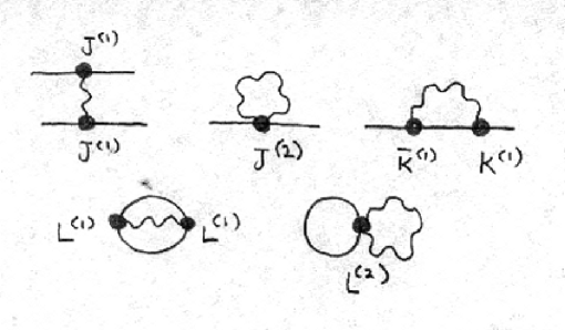
Figure 2: second order perturbation theory

With this preliminary calculation out of the way we are now ready to state:

Theorem 2

$${\cal Z}^{*}_{\Theta}=\exp\left(P_{\Theta}+\sum_{X\cap\Theta\neq\emptyset}E^{**}(X)\right)$$ (243)

The functions $E^{**}(X)$ are translation covariant inside $\Theta$ and for any $\epsilon>0$ we have

$$\|E^{**}(X)\|_{h_{1}}\leq{\cal O}(e_{0}^{4-\epsilon})e^{-\kappa|X|_{1}}$$ (244)

also in the kernel norm.

Proof. We expand $\log{\cal Z}_{\Theta}^{*}=\log{\cal Z}(1)$ by

$$\log{\cal Z}(1)=\log{\cal Z}(0)+\frac{1}{2!}(\log{\cal Z})^{{}^{\prime\prime}}(0)++\frac{1}{3!}\int_{0}^{1}(1-t)^{3}(\log{\cal Z})^{{}^{\prime\prime\prime\prime}}(t)dt$$ (245)

To treat the remainder term we use the expansion $\log{\cal Z}(t)=\sum_{X}E(t,X)$ from (240). This gives a contribution $\frac{1}{3!}\int_{0}^{1}(1-t)^{3}E^{{}^{\prime\prime\prime\prime}}(t,X)dt$ to $E^{**}(X)$. To analyze this term we first claim $E(t,X)$ is actually analytic in complex $|t|\leq e_{0}^{-1+\epsilon}$ with a weaker bound. This follows because $t$ enters V(t) either in the combination $e^{ite_{0}A_{0}}-1$ for the main terms or $t^{2}e_{0}$ for the counterterms. In the first case we have our characteristic function enforcing that $|A_{0}|\leq{\cal O}(p(e_{0}))$ and thus this factor is ${\cal O}(e_{0}^{\epsilon}p(e_{0}))$. The counterterms are ${\cal O}(e_{0}^{2\epsilon})$. Altogether we have that $V(t)$ is ${\cal O}(e_{0}^{\epsilon}p(e_{0}))$. This carries through the proof of theorem 1 and yields $\|E(t,X)\|_{h_{1}}\leq{\cal O}(e_{0}^{\epsilon}p(e_{0})e^{-\kappa|X|_{1}})$ for $|t|\leq e_{0}^{-1+\epsilon}$ Now returning to $0\leq t\leq 1$ and using a Cauchy bound we have for the fourth derivative $\|E^{{}^{\prime\prime\prime\prime}}(t,X)\|_{h_{1}}\leq{\cal O}(e_{0}^{4-3\epsilon}p(e_{0})e^{-\kappa|X|_{1}})$. Since $p(e_{0})\leq e_{0}^{-\epsilon}$ and $\epsilon$ is arbitrary we can take this to be ${\cal O}(e_{0}^{4-\epsilon}e^{-\kappa|X|_{1}})$ as claimed.

Next consider the second order term. This time we do not use (240) but instead use the global representation (239). Thus we almost get the terms we computed in (241), but now we must deal with the characteristic functions. We compute

$$\frac{1}{2}(\log{\cal Z})^{{}^{\prime\prime}}(0)=\frac{1}{2}\frac{\int\left(V^{\prime}(0)^{2}-V^{\prime\prime}(0)\right)\chi^{*}(\Theta,A_{0})\ d\mu_{\stackrel{{\scriptstyle}}{{C^{loc}}}}(A_{0})\ d\mu_{\stackrel{{\scriptstyle}}{{\Gamma^{loc}(\tilde{A})}}}(\Psi_{0})}{\int\chi^{*}(\Theta,A_{0})\ d\mu_{\stackrel{{\scriptstyle}}{{C^{loc}}}}(A_{0})}$$ (246)

The four-fermion part of this is

$$\frac{1}{2}\sum_{x,y\in\Theta}J^{(1)}_{\mu}(x)J^{(1)}_{\mu}(y)C^{loc}_{\chi}(x,y)$$ (247)

where (no sum on $\mu$)

$$C^{loc}_{\chi}(x,y)=\frac{\int A_{\mu,0}(x)A_{\mu,0}(y)\chi^{*}(\Theta,A_{0})\ d\mu_{\stackrel{{\scriptstyle}}{{C^{loc}}}}(A_{0})}{\int\chi^{*}(\Theta,A_{0})\ d\mu_{\stackrel{{\scriptstyle}}{{C^{loc}}}}(A_{0})}$$ (248)

We claim that this can be written as $C^{loc}(x,y)$ plus something tiny with good decay. This follows by another cluster expansion which we outline in Appendix D. For us the most useful way to state it is

$$C^{loc}_{\chi}(x,y)=C^{loc}(x,y)+\sum_{X\ni x,y}\delta K_{xy}(X)$$ (249)

where $|\delta K_{xy}(X)|\leq{\cal O}(e^{-{\cal O}(1)p(e_{0})^{2}})e^{-2\kappa|X|_{1}}$. Inserting this in (247) the first term contributes to $P_{\Theta}$. The second term gives a contribution to $E^{**}(X)$ which is

$$\sum_{x,y\in X\cap\Theta}J^{(1)}_{\mu}(x)J^{(1)}_{\mu}(y)\delta K_{xy}(X)$$ (250)

and this has the bound ${\cal O}(e_{0}^{4-\epsilon}e^{-\kappa|X|_{1}})$ as claimed.

The treatment of the other terms in (246) is similar in each case splitting into a contribution to $P_{\Theta}$ and a contribution to $E^{**}$. The fermion propagator must also be localized with an expansion (see lemma 16)

$$\Gamma^{loc}(\tilde{A};x,y)=\sum_{X\ni x,y}\Gamma_{X}^{loc}(\tilde{A};x,y)$$ (251)

for its contribution to $E^{**}(X)$.

Finally consider the zeroth order term $\log Z(0)$. Again we use (240): $\log{\cal Z}(0)=\sum_{X}E(0,X)$. Now there is no potential. The only contributions to $E(0,X)$ are from the characteristic functions. This means lemma 8 can be modified to obtain a factor ${\cal O}(e^{-{\cal O}(1)p(e_{0})^{2}})$ instead of ${\cal O}(e_{0}p(e_{0}))$. Hence $E(0,X)$ is ${\cal O}(e^{-{\cal O}(1)p(e_{0})^{2}})e^{-\kappa|X|_{1}}$. These terms contribute to $E^{**}(X)$.

4.6 final adjustments

Assembling the results of the previous two sections we have for the small field region

$${\cal Z}^{\dagger}=\exp\left(P_{\Theta}+\sum_{X\cap\Theta\neq\emptyset}E^{**}(X)\sum_{X\cap\Theta\neq\emptyset,X\subset(\Theta^{\prime\prime})^{c}}B^{\#}(X)+\sum_{X\cap\Theta\neq\emptyset}R^{\prime}(X)\right)$$ (252)

where $R^{\prime}(X)=R^{\#}(X)+R^{*}(X)$.

It will be convenient to remove the $R^{\prime}$ from the small field region. It is possible because $R^{\prime}$ is so tiny. We make another Mayer expansion and write

$$\exp\left(\sum_{X\cap\Theta\neq\emptyset}R^{\prime}(X)\right)=\sum_{\{X_{i}\}}\prod_{i}(e^{R^{\prime}(X_{i})}-1)=\sum_{S}U(S)$$ (253)

where $\{X_{i}\}$ are distinct connected sets and where

$$U(S)=\sum_{\{X_{i}\}:\cup X_{i}=S}\prod_{i}(e^{R^{\prime}(X_{i})}-1)$$ (254)

The function $U(S)$ factors over its connected components each one of which must intersect $\Theta$. From the bound on $R^{\prime}(X)$ we have for $S$ connected

$$\|U(S)\|_{h_{1}}\leq{\cal O}(e^{-r(e_{0})/M_{1}})e^{-{\cal O}(1)\kappa|S|}$$ (255)

This is sufficient to control the sum over $S$. Now we write

$$\sum_{S}U(S)=\sum_{\Upsilon\subset\Theta}\left(\sum_{S:\Theta-S=\Upsilon}U(S)\right)\equiv\sum_{\Upsilon\subset\Theta}{\cal U}(\Upsilon^{c})$$ (256)

Let us return to the full fluctuation integral (148). This can now be written

$$\tilde{\Xi}_{\Lambda}=\sum_{\Upsilon\subset\Theta\subset\Lambda^{\prime}}{\cal G}_{\Theta,\Upsilon}\ \ \exp\left(P_{\Theta}+\sum_{X\cap\Theta\neq\emptyset}E^{**}(X)\right)$$ (257)

where we have defined

$${\cal G}_{\Theta,\Upsilon}={\cal T}(\Theta^{c})\exp\left(\sum_{X\cap\Theta\neq\emptyset,X\subset(\Theta^{\prime\prime})^{c}}B^{\#}(X)\right){\cal U}(\Upsilon^{c})$$ (258)

We make the inverse transformation $A_{0}\to A_{0}-[H_{1}^{loc}A]_{\Omega^{\prime}}$ in $\Lambda^{c}$ and similarly for fermions. This does not affect the exponential and changes ${\cal G}_{\Theta,\Upsilon}$ to ${\cal G}^{\prime}_{\Theta,\Upsilon}$ whence

$$\tilde{\Xi}^{\prime}_{\Lambda}=\sum_{\Upsilon\subset\Theta\subset\Lambda^{\prime}}{\cal G}^{\prime}_{\Theta,\Upsilon}\ \ \exp\left(P_{\Theta}+\sum_{X\cap\Theta\neq\emptyset}E^{**}(X)\right)$$ (259)

Next we scale replacing $A$ by $A_{1,L}$ , etc. to obtain

$$\Xi_{1,\Lambda}=\sum_{\Upsilon\subset\Theta\subset\Lambda^{\prime}}{\cal G}_{1,\Theta,\Upsilon}\ \ \exp\left({\cal P}_{1,L^{-1}\Theta}+\sum_{Y\cap L^{-1}\Theta\neq\emptyset}E_{1}(Y)\right)$$ (260)

where ${\cal G}_{1,\Theta,\Upsilon}$ is the scaled version of ${\cal G}^{\prime}_{\Theta,\Upsilon}$. We have also defined

$$\begin{split}{\cal P}_{1,L^{-1}\Theta}(\psi_{1}({\cal A}_{1}),{\cal A}_{1})=&P_{\Theta}([\psi_{1}({\cal A}_{1})]_{L},{\cal A}_{1,L})\\ E_{1}(Y,\psi_{1}({\cal A}_{1}),{\cal A}_{1})=&\sum_{X:\bar{X}^{L}=LY,X\cap\Theta\neq\emptyset}E^{**}(X,[\psi_{1}({\cal A}_{1})]_{L},{\cal A}_{1,L})\\ \end{split}$$ (261)

Here $\bar{X}^{L}$ is the smallest union of of $LM_{1}$ blocks containing $X$. Explicitly we have for $S\subset{\mathbb{T}}^{-1}_{N+M-1}$

$$\begin{split}&{\cal P}_{1,S}(\tilde{\Psi}(\tilde{A}),\tilde{A})\\ =&\frac{1}{2}L^{-6}\sum_{x,y\in S}{\cal J}^{(1)}_{\mu}(x)G^{loc}_{1}(x,y){\cal J}^{(1)}_{\mu}(y)-\frac{1}{2}L^{-4}\sum_{x\in S}{\cal J}^{(2)}_{\mu,\mu}(x,x)G^{loc}_{1}(x,x)\\ +&\frac{1}{2}L^{-6}\sum_{x,y,z,w\in S}\bar{\cal K}^{(1)}_{\mu}(z,x)S^{loc}_{1}({\cal A}_{1};z,w){\cal K}^{(1)}_{\mu}(w,y)\ G^{loc}_{1}(x,y)\\ -&\frac{1}{2}L^{-6}\sum_{x,y,z,w\in S}{\cal K}^{(1)}_{\mu}(z,x)S^{loc}_{1}({\cal A}_{1};z,w)\bar{\cal K}^{(1)}_{\mu}(w,y)\ G^{loc}_{1}(x,y)\\ -&L^{-6}\sum_{x,y,z,z^{\prime},w,w^{\prime}\in S}tr\left({\cal L}^{(1)}_{\mu}(z,z^{\prime},x)S^{loc}_{1}({\cal A}_{1};z^{\prime},w^{\prime}){\cal L}^{(1)}_{\mu}(w^{\prime},w,y)S^{loc}_{1}({\cal A}_{1};w,z)\right)G^{loc}_{1}(x,y)\\ -&\frac{1}{2}L^{-4}\sum_{x,y,z,z^{\prime}\in S}tr\left({\cal L}^{(2)}_{\mu}(z,z^{\prime},x,x)S^{loc}_{1}({\cal A}_{1};z^{\prime},z)\right)G^{loc}_{1}(x,x)\\ -&L^{-3}\sum_{x\in S}:\bar{\psi}_{1}({\cal A}_{1},x)\ \delta m_{1}\ \psi({\cal A}_{1},x):_{\hat{S}_{1}-{\cal S}_{1}^{loc}({\cal A}_{1})}-\delta cE_{1}^{\prime}|S|\\ \end{split}$$ (262)

Here $\hat{S}_{1}=(D(0)+m_{1})^{-1},m_{1}=Lm_{0},\delta m_{1}=L\delta m_{0}$, and $\delta{\cal E}^{\prime}_{1}=L^{3}\delta{\cal E}_{0}$. The vertices ${\cal J}^{(n)},{\cal K}^{(n)},{\cal L}^{(n)}$ are the scaled versions of $J^{(n)},K^{(n)},L^{(n)}$. For example

$${\cal J}_{\mu}^{(1)}(x,\psi_{1}({\cal A}_{1}),{\cal A}_{1})=L^{5/2}J_{\mu}^{(1)}(Lx,[\psi_{1}({\cal A}_{1})]_{L},{\cal A}_{1,L})$$ (263)

In general $J^{(n)},K^{(n)},L^{(n)}$ have the scaling factors $L^{2+\frac{1}{2}n},L^{1+\frac{1}{2}n},L^{\frac{1}{2}n}$. With this choice and $e_{1}=L^{1/2}e_{0}$ we have that $J^{(n)},K^{(n)},L^{(n)}$ are ${\cal O}(e_{1}^{n})$. We have also introduced

$$\begin{split}G^{loc}_{1}(x,y)=&LC^{loc}(Lx,Ly)\\ S^{loc}_{1}({\cal A}_{1};x,y)=&L^{2}\Gamma^{loc}_{0}({\cal A}_{1,L};Lx,Ly)\\ \end{split}$$ (264)

which are local approximations to the propagators $G_{1},S_{1}({\cal A}_{1})$ defined earlier

5 Summary

Now insert the expression (260) for the fluctuation integral into our expansion (121) and obtain the density on ${\mathbb{T}}^{0}_{N+M-1}$

$$\begin{split}\rho_{1}(\Psi_{1},A_{1})=&c_{0}e^{-\delta E_{1}}\sum_{\Omega,\tilde{\Lambda},\Theta,\Upsilon}\int d\Psi_{0}dA_{0}\ \zeta_{1,\Omega,\tilde{\Lambda}}\ \chi_{1,\Omega,\tilde{\Lambda}}\ {\cal G}_{1,\Theta,\Upsilon}\ \\ &\exp\left(-\frac{a}{2L^{2}}|A_{1,L}-QA_{0}|^{2}-\frac{1}{2}(A_{0},(-\Delta+\mu_{0}^{2})A_{0})\right)\\ &\exp\left(-\frac{a}{L}|\Psi_{1,L}-Q_{e_{0}}(\hat{A}_{1})\Psi_{0}|^{2}-(\bar{\Psi}_{0},(D_{e_{0}}(\hat{A}_{1})+m_{0})\Psi_{0})\right)\ \\ &\exp\left({\cal P}_{1,L^{-1}\Theta}+\sum_{X\cap L^{-1}\Theta\neq\emptyset}E_{1}(X)\right)\chi_{1}(L^{-1}\Omega^{\prime\prime},A_{1})\\ \end{split}$$ (265)

The sum is over decreasing sets $\Omega\supset\tilde{\Lambda}\supset\Theta\supset\Upsilon$ (which however are not the only restrictions). The factor $\zeta_{1,\Omega,\tilde{\Lambda}}\ \chi_{1,\Omega,\tilde{\Lambda}}\ {\cal G}_{1,\Theta,\Upsilon}$ supplies the convergence factors for the sums and is localized in $\Upsilon^{c}$. The function ${\cal P}_{1}+\sum_{X}E_{1}(X)$ is the effective action for the small field region with second order perturbation theory isolated.

This completes the treatment of the first step. In next paper we take these expressions as a starting point and iterate the operations we have performed. After $k$ steps we are on the smaller torus ${\mathbb{T}}_{N+M-k}$ and we have an expansion similar to the above now with $4k$ decreasing sums over regions. In the new small field we have an effective action ${\cal P}_{k}+\sum_{X}E_{k}(X)$. The function ${\cal P}_{k}$ is second order in a running coupling constant $e_{k}=L^{-(N-k)/2}e$. It is given by the same diagrams as ${\cal P}_{1}$ but is expressed on the finer lattice ${\mathbb{T}}^{-k}_{N+M-k}$ instead of ${\mathbb{T}}^{-1}_{N+M-1}$.

As $k$ gets large the ultraviolet singularities begin to appear again. In ${\cal P}_{k}$ the effect is denied by explicit renormalization cancellations. One can perhaps see how this will develop already in (262). In higher orders the effect is reflected in the fact that every time we scale down we potentially gain a factor of $L^{3}$ (see (261)). This is handled by the scaling properties of the fermion fields and the allowed growth of the coupling constant. In this respect our analysis is more like [11]. The case of no fermion fields is special. We take out the constant part with the energy counterterm and then locally we use gauge invariance to regard it as a function of the field strength $dA$. This has sufficiently good scaling properties to control the growth, see [15]. Thus the UV problems are handled. The IR problems are also disappearing as $k\to N$ since the volume is shrinking. Thus we will get an expression which is uniformly bounded in $N$.

Appendix A random walk expansions

We quote/sketch some results on the covariance operators. The original treatment for the Laplacian is due to Balaban [4] and the treatment for the Dirac operator can be found in Balaban, O’Carroll, and Schor [9], [10]. The operators on a unit lattice ${\mathbb{T}}^{0}_{N}$ are

$$\begin{split}C_{\Lambda}=&[\Delta^{\#}]_{\Lambda}^{-1}=[-\Delta+\mu_{0}^{2}+\frac{a}{L^{2}}Q^{T}Q]_{\Lambda}^{-1}\\ \Gamma_{\Lambda}(A)=&[D^{\#}(A)]_{\Lambda}^{-1}=[D_{e_{0}}(A)+m_{0}+\frac{a}{L}Q_{e_{0}}(-A)^{T}Q_{e_{0}}(A)]_{\Lambda}^{-1}\\ \end{split}$$ (266)

Here $\Lambda$ is a union of $M_{0}$-cubes centered on the $M_{0}$ lattice ${\mathbb{T}}^{M_{0}}_{N}$. The operators $[-\Delta]_{\Lambda}$ and $[D(A)]_{\Lambda}$ are defined by restricting to bonds in $\Lambda$. For the Laplacian this means Neumann boundary conditions.

First consider $C_{{\cal O}},\Gamma_{{\cal O}}(A)$ where ${\cal O}$ is one of the sets ${\cal O}_{j}$ defined for $j\in T^{M_{0}}_{N}$ by

$${\cal O}_{j}=\{x\in\Lambda:|x-j|\leq M_{0}\}$$ (267)

Here $|x-j|=\sup_{\mu}|x_{\mu}-j_{\mu}|$. These overlap and cover $\Lambda$. For interior points ${\cal O}_{j}$ is a $2M_{0}$ cube. Let $\|\partial A\|_{{\cal O}}=\sup_{{\cal O}}|\partial A|$

Lemma 13

Let $e_{0}M_{0}L^{2}\|\partial A\|_{{\cal O}}$ be sufficiently small. Then $\Gamma_{{\cal O}}(A)$, $C_{{\cal O}}$ exist and

$$\begin{split}\|\Gamma_{{\cal O}}(A)f\|_{2}\leq&{\cal O}(L^{2})\|f\|_{2}\\ \|C_{{\cal O}}f\|_{2}\leq&{\cal O}(L^{2})\|f\|_{2}\\ \end{split}$$ (268)

Proof. The bounds on $C_{{\cal O}}$ follow from the lower bound $(f,[-\Delta+aL^{-2}Q^{T}Q]_{{\cal O}}f)\geq{\cal O}(L^{-2})\|f\|^{2}$. This in turn follows by bounding it below by a sum over $L$-squares with Neumann conditions. On each $L$-square $Q^{T}Q$ projects onto constants and on the complement of the constants the Laplacian is bounded below by ${\cal O}(L^{-2})$. See [4]. The bound for $\Gamma_{{\cal O}}(0)$ can be reduced to a bound on the Laplacian. See [10], lemma VI.4 for general idea.

lf $A_{0}$ is a constant (possibly large) we have on ${\cal O}$ that $A_{0}=\partial\lambda_{0}$. Then by the gauge covariance

$$\Gamma_{{\cal O}}(A_{0})=e^{ie_{0}\lambda_{0}}\Gamma_{{\cal O}}(0)e^{-ie_{0}\lambda_{0}}$$ (269)

Hence we have the result for constant background field.

Now in general for a field A on ${\cal O}$ we can write $A=\bar{A}+\delta A$ where $\bar{A}$ = constant is the average over ${\cal O}$ and $|\delta A|\leq M\|\partial A\|_{{\cal O}}$. Then put $V=D^{\#}_{{\cal O}}(\bar{A}+\delta A)-D^{\#}_{{\cal O}}(\bar{A})$ This has the contribution (34) from $D_{e_{0}}(A)$, and also a contribution from $Q_{e_{0}}(-A)^{T}Q_{e_{0}}(A)$. For $x\in B(y)$ we have the explicit formula

$$\left(Q(-A)^{T}Q(A)f\right)(x)=L^{-3}\sum_{\tilde{x}\in B(y)}\exp\left(ie_{0}A(\Gamma_{xy}\cup\Gamma_{y\tilde{x}})\right)f(\tilde{x})$$ (270)

Using these expressions we find

$$\|Vf\|_{2}\leq{\cal O}(1)(e_{0}M_{0}\|\partial A\|_{{\cal O}})\|f\|_{2}$$ (271)

Under our assumptions the inverse exists and is given by

$$\Gamma_{{\cal O}}(\bar{A}+\delta A)=\Gamma_{{\cal O}}(\bar{A})\sum_{n-0}^{\infty}(-V\ \Gamma_{{\cal O}}(\bar{A}))^{n}$$ (272)

with the bound

$$\|\Gamma_{{\cal O}}(\bar{A}+\delta A)f\|_{2}\leq{\cal O}(L^{2})(1-e_{0}M_{0}L^{2}\|\partial A\|_{{\cal O}})^{-1}\|f\|_{2}\leq{\cal O}(L^{2})\|f\|_{2}$$ (273)

This completes the proof.

We turn to the case of general $\Lambda$. Now inverses are obtained by a random walk expansion. A path $\omega$ in $\Lambda$ is a sequence of lattice point $\omega=(j_{0},j_{1},\dots,j_{n})$ which are neighbors in the sense that $|j_{\alpha}-j_{\alpha+1}|=0$ or $M_{0}$ for any adjacent pair $(j_{\alpha},j_{\alpha+1})$. The length of the path is $\ell(\omega)=n$. Each path $\omega$ also determines a sequence of cubes $({\cal O}_{j_{0}},{\cal O}_{j_{1}},\cdots,{\cal O}_{j_{n}})$ as defined above. A path connects points $x,y$ in the unit lattice if $x\in{\cal O}_{j_{0}}$ and $y\in{\cal O}_{j_{n}}$ in which case we write $\omega:x\to y$.

Lemma 14

Let $L^{2}/M_{0}$ and $e_{0}M_{0}L^{2}\|\partial A\|_{{\cal O}}$ be sufficiently small.

1. $\Gamma_{\Lambda}(A)$ and $C_{\Lambda}$ exist.

2. We have the random walk expansion

   $$\begin{split}\Gamma_{\Lambda}(A)=&\sum_{\omega}\Gamma_{\Lambda,\omega}(A)\\ C_{\Lambda}=&\sum_{\omega}C_{\Lambda,\omega}\\ \end{split}$$ (274)

   The kernels $\Gamma_{\Lambda,\omega}(A,x,y)$ and $C_{\Lambda,\omega}(x,y)$ vanish unless $\omega:x\to y$ and satisfy for some constant $\alpha$

   $$\begin{split}|C_{\Lambda,\omega}(x,y)|\leq&{\cal O}(L^{2})(\frac{\alpha L^{2}}{M_{0}})^{\ell(\omega)}\\ |\Gamma_{\Lambda,\omega}(A,x,y)|\leq&{\cal O}(L^{2})(\frac{\alpha L^{2}}{M_{0}})^{\ell(\omega)}\\ \end{split}$$ (275)

3. $\Gamma_{\Lambda,\omega}(A)$ depends on $A$ only in ${\cal O}_{j_{0}}\cup\dots\cup{\cal O}_{j_{n}}$.

Proof. We give the results for the Dirac operator. First suppose $\Lambda$ is the whole torus $T^{0}_{N}$ and denote $\Gamma_{\Lambda}(A)$ as just $\Gamma(A)$. Choose smooth $g$ with support in $\{x:|x|\leq\frac{2}{3}\}$ so that $g=1$ on $\{x:|x|\leq\frac{1}{3}\}$ and so that $\sum_{i\in{\mathbb{Z}}^{3}}g^{2}(x-i)=1$. Then for $j\in T^{M_{0}}_{N}$ define $h_{j}(x)=g((x-j)/M_{0})$. Then $h_{j}$ is supported in $\{x:|x-j|\leq\frac{2}{3}M_{0}\}\subset{\cal O}_{j}$ and $h_{j}=1$ on $\{x:|x-j|\leq\frac{1}{3}M_{0}\}$ and $\sum_{j}h_{j}^{2}=1$. We define a parametrix by

$$\Gamma^{*}(A)=\sum_{j}h_{j}\Gamma_{{\cal O}_{j}}(A)h_{j}$$ (276)

Here things are arranged to avoid potential discontinuities of $\Gamma_{{\cal O}_{j}}(x,y)$ for $(x,y)$ on the boundary of ${\cal O}_{j}$. Since $D^{\#}(A)\Gamma_{{\cal O}_{j}}(A)=I$ inside ${\cal O}_{j}$ we have

$$D^{\#}(A)\Gamma^{*}(A)=I-\sum_{j}R_{j}(A)\Gamma_{{\cal O}_{j}}(A)h_{j}\equiv I-R(A)$$ (277)

where

$$R_{j}(A)=-\left[D^{\#}(A),h_{j}\right]$$ (278)

The inverse of $D^{\#}(A)$ is now

$$\Gamma(A)=\Gamma^{*}(A)(I-R(A))^{-1}=\Gamma^{*}(A)\sum_{n=0}^{\infty}R(A)^{n}$$ (279)

with convergence in $\ell^{2}$ provided $\|R(A)\|<1$.

To see this we develop some estimates. For $R_{j}(A)$ we note that $\|[D_{e_{0}}(A),h_{j}]\|={\cal O}(M_{0}^{-1})$ since $|\partial h_{j}|\leq{\cal O}(M_{0}^{-1})$. Furthermore we compute for $x\in B(y)$

$$\begin{split}&\frac{a}{L}\left([Q(-A)^{T}Q(A),h_{j}]f\right)(x)\\ &L^{-3}\sum_{\tilde{x}\in B(y)}\exp\left(ie_{0}A(\Gamma_{xy}\cup\Gamma_{y\tilde{x}})\right)\frac{a}{L}(h_{j}(x)-h_{j}(\tilde{x}))f(\tilde{x})\\ \end{split}$$ (280)

Again this is bounded by $|\partial h_{j}|$ and so $(a/L)\|[Q(-A)^{T}Q(A),h_{j}]\|={\cal O}(M_{0}^{-1})$. Combining these bounds we have $\|R_{j}(A)\|\leq{\cal O}(M_{0}^{-1})$. Note also that functions in the range of $R_{j}(A)$ have support in ${\cal O}_{j}$ since $L$ is much smaller than $M_{0}$.

Now we have since $h_{i}R_{j}(A)=0$ unless $i,j$ are neighbors

$$\|h_{i}Rf\|\leq\sum_{j}\|h_{i}R_{j}(A)\Gamma_{{\cal O}_{j}}(A)h_{j}f\|\leq{\cal O}(L^{2}M_{0}^{-1})\sum_{j:|i-j|\leq M_{0}}\|h_{j}f\|$$ (281)

After a Schwarz inequality we can replace the sum on the right by the expression $(\sum_{j:|i-j|\leq M_{0}}\|h_{j}f\|^{2})^{1/2}$. Then

$$\|R(A)f\|^{2}=\sum_{i}\|h_{i}R(A)f\|^{2}\leq{\cal O}(L^{4}M_{0}^{-2})\sum_{i,j:|i-j|\leq M_{0}}\|h_{j}f\|^{2}\leq{\cal O}(L^{4}M_{0}^{-2})\|f\|^{2}$$ (282)

Hence $\|R(A)\|\leq{\cal O}(L^{2}M_{0}^{-1})<1$ and (a.) is proved.

Now we can write $\Gamma(A)$ as a sum over random walks by inserting the definitions of $\Gamma^{*}(A)$ and $R(A)$ into (279) and obtaining

$$\begin{split}\Gamma(A)=&\sum_{n=0}^{\infty}\sum_{j_{0},j_{1},...,j_{n}}(h_{j_{0}}\Gamma_{{\cal O}_{j_{0}}}(A)h_{j_{0}})(R_{j_{1}}(A)\Gamma_{{\cal O}_{j_{1}}}(A)h_{j_{1}})\cdots(R_{j_{n}}(A)\Gamma_{{\cal O}_{j_{n}}}(A)h_{j_{n}})\\ \equiv&\sum_{\omega}\Gamma_{\omega}(A)\\ \end{split}$$ (283)

Here in the last step we notice that we get zero unless $j_{\alpha},j_{\alpha+1}$ are neighbors.

By our previous estimates we have for some $\alpha={\cal O}(1)$

$$\|\Gamma_{\omega}(A)\|\leq{\cal O}(L^{2})(\alpha L^{2}/M_{0})^{\ell(\omega)}$$ (284)

Since we are on a unit lattice the same bound holds for $|\Gamma_{\omega}(A,x,y)|$. The restriction to $\omega:x\to y$ is obvious. Thus (b.) is proved and (c.) follows by inspection.

Now suppose consider general $\Lambda$. We replace $h_{j}$ by $h^{\Lambda}_{j}\equiv\chi_{\Lambda}h_{j}$ and repeat the above argument with $[D^{\#}(A)]_{\Lambda}$ instead of $D^{\#}(A)$. This completes the proof.

Remark. If $\omega$ has no points on $\partial\Lambda$ then $C_{\Lambda,\omega}$ and $\Gamma_{\Lambda,\omega}(A)$ are independent of $\Lambda$.

Lemma 15

Under the same assumptions with $\beta=M_{0}^{-1}$ we have for $x,y\in\Lambda$.

$$\begin{split}|C_{\Lambda}(x,y)|&\leq{\cal O}(L^{2})exp(-\beta d(x,y))\\ |\Gamma_{\Lambda}(A;x,y)|&\leq{\cal O}(L^{2})exp(-\beta d(x,y))\\ \end{split}$$ (285)

Also

$$|\Gamma_{\Lambda}(A;x,y)-\Gamma(A;x,y)|\leq{\cal O}(L^{2})exp\left(-\beta(d(x,y)+d(x,\Lambda^{c})+d(y,\Lambda^{c}))\right)$$ (286)

and similarly for $C_{\Lambda}(x,y)$.

Proof. A crude estimate is

$$\begin{split}\Gamma_{\Lambda}(A;x,y)\leq&{\cal O}(L^{2})\sum_{\omega:x\to y}(\frac{\alpha L^{2}}{M_{0}})^{\ell(\omega)}\\ \leq&{\cal O}(L^{2})\sum_{n}(\frac{\alpha L^{2}}{M_{0}})^{n}|\{\omega:x\to y:\ell(\omega)=n\}|\\ \leq&{\cal O}(L^{2})\sum_{n}(\frac{27\alpha L^{2}}{M_{0}})^{n}\leq{\cal O}(L^{2})\\ \end{split}$$ (287)

But the condition $\omega:x\to y$ means that the sum is restricted to $n\geq(d(x,y)/M_{0})-2$. Thus we can estimate $(\alpha L^{2}M_{0}^{-1})^{n/2}$ by ${\cal O}(1)\exp(-d(x,y)/M_{0})$ and still have another factor $(\alpha L^{2}M_{0}^{-1})^{n/2}$ to estimate the sum as above.

For the second result proceed as follows. We write

$$\Gamma_{\Lambda}(A;x,y)-\Gamma(A;x,y)=\sum_{\omega:x\to y}\Gamma_{\Lambda,\omega}(A;x,y)-\Gamma_{\omega}(A;x,y)$$ (288)

But if $\omega$ has no boundary points we have $\Gamma_{\Lambda,\omega}(A,x,y)=\Gamma_{\omega}(A,x,y)$ and hence no contribution. Thus we can restrict to $\omega$ with boundary points and hence get the result for each term separately.

We will also need reblocked random walk expansions on a scale $M_{1}$ larger than $M_{0}$. We assume $\Lambda$ is a union of $M_{1}$ blocks centered on ${\mathbb{T}}^{M_{1}}_{N}$ and we have

Lemma 16

Under the same assumptions

$$\begin{split}C_{\Lambda}=&\sum_{X\ni x,y}C_{\Lambda,X}\\ \Gamma_{\Lambda}(A)=&\sum_{X\ni x,y}\Gamma_{\Lambda,X}(A)\\ \end{split}$$ (289)

where the sum is over connected unions of $M_{1}$-blocks $X$. The operator $\Gamma_{\Lambda,X}(A)$ depends on $A$ only in X and the kernels $C_{\Lambda}(x,y),\Gamma_{\Lambda}(A,x,y)$ have support in $X\times X$. Furthermore

$$\begin{split}|C_{\Lambda,X}(x,y)|\leq&{\cal O}(1)e^{-\beta M_{1}|X|_{1}}e^{-\beta d(x,y)}\\ |\Gamma_{\Lambda,X}(A,x,y)|\leq&{\cal O}(1)e^{-\beta M_{1}|X|_{1}}e^{-\beta d(x,y)}\\ \end{split}$$ (290)

Proof. Define

$$\Gamma_{\Lambda,X}(A,x,y)=\sum_{\stackrel{{\scriptstyle\omega:x\to y}}{{\bar{\omega}=X}}}\Gamma_{\Lambda,\omega}(A,x,y)$$ (291)

where $\bar{\omega}$ are the $M_{1}$ blocks intersecting ${\cal O}_{j_{0}}\cup\dots\cup{\cal O}_{j_{n}}$. Now $\bar{\omega}$ cannot be very large without $\omega$ itself covering some substantial distance and one can show

$$M_{0}\ell(\omega)\geq 9M_{1}(|\bar{\omega}|_{1}-8)$$ (292)

Using this for a lower bound on $\ell(\omega)$ we extract the factor $e^{-\beta M_{1}|X|_{1}}$. The estimate now proceeds as before. This completes the proof.

We also want to consider local operators $C^{loc}_{\Lambda}(x,y)$ and $\Gamma^{loc}_{\Lambda}(A,x,y)$ defined by restricting the random walk expansion (274) to paths which stay within $r(e_{0})/2$ of both $x$ and $y$. Then we have

Lemma 17

Under the same assumptions

$$\begin{split}C_{\Lambda}-C^{loc}_{\Lambda}=&\sum_{X}\delta C_{\Lambda,X}\\ \Gamma_{\Lambda}(A)-\Gamma^{loc}_{\Lambda}(A)=&\sum_{X}\delta\Gamma_{\Lambda,X}(A)\\ \end{split}$$ (293)

where

$$\begin{split}|\delta C_{\Lambda,X}(x,y)|\leq&{\cal O}(e^{-\beta r(e_{0})})e^{-\beta M_{1}|X|_{1}}e^{-\beta d(x,y)}\\ |\delta\Gamma_{\Lambda,X}(A,x,y)|\leq&{\cal O}(e^{-\beta r(e_{0})})e^{-\beta M_{1}|X|_{1}}e^{-\beta d(x,y)}\\ \end{split}$$ (294)

Proof. $\delta\Gamma_{\Lambda,X}(A,x,y)$ has an expression like (291) in which only paths with $\ell(\omega)\geq M_{0}^{-1}r(e_{0})/2$ contribute. This enables us to extract the factor $e^{-\beta r(e_{0})}$.

Finally we consider operators of the form $\partial C_{\Lambda}(s)/\partial s_{Y}$ as defined in the text in (159)

Lemma 18

Let ${\cal L}(x,y,Y)$ is the length of the shortest tree through $x,y$ and the centers of the blocks in $Y$. Then with a universal constant ${\cal O}(1)$ we have

$$\begin{split}|\frac{\partial C_{\Lambda}}{\partial s_{Y}}(x,y)|\leq&{\cal O}(1)M_{0}^{-{\cal O}(1)|Y|_{1}}e^{-\beta{\cal L}(x,y,Y)}\\ \end{split}$$ (295)

and similarly for fermions.

Proof. We can assume $Y\neq\emptyset$. We have $C_{\Lambda}(s,x,y)=\sum_{\omega:x\to y}s_{\omega}C_{\Lambda,\omega}(x,y)$. After the $\partial/\partial s_{Y}$ differentiation the only terms $\omega$ which survive are those with with $\ell(\omega)\geq 1$ and $\bar{\omega}\supset\Delta_{x}\cup\Delta_{y}\cup Y$ where $\Delta_{x}$ is the $M_{1}$ block containing $x$. This leads to

$$|\frac{\partial C_{\Lambda}}{\partial s_{Y}}(x,y)|\leq{\cal O}(L^{2})\sum_{\omega}{}^{\prime}(\frac{\alpha L^{2}}{M_{0}})^{\ell(\omega)}$$ (296)

The prime indicates the restricted sum over paths. Now $\ell(\omega)\geq|\bar{\omega}|_{1}/2\geq|Y|_{1}/2-1$ enables us to extract a factor $M_{0}^{-{\cal O}(1)|Y|_{1}}$. (For the first inequality assume $|\bar{\omega}|_{1}\geq 2$ and use $\ell(\omega)\geq|\bar{\omega}|_{1}-1\geq|\bar{\omega}|/2$; check $|\bar{\omega}|_{1}=1$ separately). On the other hand by (292) and the fact that $\bar{\omega}$ is connected we have

$$M_{0}\ell(\omega)\geq 9M_{1}|\bar{\omega}|-{\cal O}(1)\geq 9{\cal L}(\bar{\omega})-{\cal O}(1)\geq{\cal O}(1){\cal L}(\Delta_{x}\cup\Delta_{y}\cup Y)-{\cal O}(1)$$ (297)

This enables us to extract a factor ${\cal O}(1)e^{-\beta{\cal L}(x,y,Y)}$.

Appendix B fermion norms and integrals

We consider the Grassman algebra generated by $\Psi_{\alpha}(x),\bar{\Psi}_{\alpha}(x)$ where $(x,\alpha)$ are spacetime and spinor indices. Let $\xi$ stand for $(0,\alpha,x)$ or $(1,\alpha,x)$ and define $\Psi(\xi)$ by $\Psi(0,\alpha,x)=\Psi_{\alpha}(x)$ and $\Psi(1,\alpha,x)=\bar{\Psi}_{\alpha}(x)$. Then the $\Psi(\xi)$ generate the algebra and any element can be uniquely written

$$F(\Psi)=\sum_{n}1/r!\sum_{\xi_{1},...,\xi_{r}}f_{r}(\xi_{1},...,\xi_{r})\Psi(\xi_{1})...\Psi(\xi_{r})$$ (298)

where the coefficients $f_{r}$ are totally antisymmetric functions. We define a norm $\|\cdot\|_{h}$ depending on a parameter $h>0$ by (c.f. [12])

$$\|F\|_{h}=\sum_{r}\frac{h^{r}}{r!}\|f_{r}\|_{1}$$ (299)

where $\|f_{r}\|_{1}$ is the $\ell_{1}$ norm.

Lemma 19

$\|FG\|_{h}\leq\|F\|_{h}\|G\|_{h}$

Proof. $H=FG$ has the coefficients

$$h_{r}=\sum_{s+t=r}\frac{r!}{s!t!}\ \textrm{alt}(f_{s}\otimes g_{t})$$ (300)

and hence

$$\|h_{r}\|_{1}\leq\sum_{s+t=r}\frac{r!}{s!t!}\ \|f_{s}\|_{1}\|g_{t}\|_{1}$$ (301)

Now multiplying by $h^{r}/r!$ and summing over $r$ gives the result.

Next consider transformations of the form $F^{\prime}(\Psi)=F(A\Psi)$ where $(A\Psi)(\xi)=\sum_{\xi^{\prime}}A(\xi,\xi^{\prime})\Psi(\xi^{\prime})$. We can estimate the effect in terms of the norm

$$\|A\|^{(1)}=\sup_{\xi}\sum_{\xi^{\prime}}|A(\xi,\xi^{\prime})|$$ (302)

Lemma 20

Let $F^{\prime}(\Psi)=F(A\Psi)$. If $h^{\prime}\|A\|^{(1)}\leq h$ then

$$\|F^{\prime}\|_{h^{\prime}}\leq\|F\|_{h}$$ (303)

Proof. $F^{\prime}$ has coefficients

$$f^{\prime}_{r}(\xi^{\prime}_{1},\dots,\xi^{\prime}_{r})=\sum_{\xi_{1},\dots,\xi_{r}}f_{r}(\xi_{1},\dots,\xi_{n})\prod_{i=1}^{r}A(\xi_{i},\xi^{\prime}_{i})$$ (304)

Hence $\|f^{\prime}_{r}\|\leq(\|A\|^{(1)})^{r}\|f_{r}\|$. Now multiply by $(h^{\prime})^{r}/r!$ and sum over $r$ to get the result.

Now we distinguish between $\Psi(x),\bar{\Psi}(x)$. We use a notation in which the spinor indices are suppressed, i.e. $x_{i}$ really means the pair $(x_{i},\alpha_{i})$. The general element (298) can then be uniquely written be in the form:

$$\begin{split}&F(\Psi,\bar{\Psi})\\ =&\sum_{n,m}\frac{1}{n!m!}\sum_{\stackrel{{\scriptstyle x_{1},...,x_{n}}}{{\bar{x}_{1},...,\bar{x}_{m}}}}f_{n,m}(x_{1},...,x_{n},\bar{x}_{1},\dots,\bar{x}_{m})\Psi(x_{1})\dots\Psi(x_{n})\bar{\Psi}(\bar{x}_{1})\dots\bar{\Psi}(\bar{x}_{m})\\ \equiv&\sum_{n,m}\frac{1}{n!m!}\sum_{X_{n},\bar{X}_{m}}f_{n,m}(X_{n},\bar{X}_{m})\Psi(X_{n})\bar{\Psi}(\bar{X}_{m})\\ \end{split}$$ (305)

where the coefficients $f_{n,m}$ are antisymmetric separately in $X_{1}=(x_{1},...,x_{n})$ and $\bar{X}_{m}=(\bar{x}_{1},...,\bar{x}_{m})$. We have in fact

$$f_{n,m}(x_{1},...,x_{n},\bar{x}_{1},\dots,\bar{x}_{m})=f_{n+m}((0,x_{1}),...,(0,x_{n}),(1,\bar{x}_{1}),\dots,(1,\bar{x}_{m}))$$ (306)

We usually consider elements in which only terms with $n=m$ contribute.

Now the norm (299) can now be written

$$\|F\|_{h}=\sum_{n,m}\frac{h^{n+m}}{n!m!}\|f_{n,m}\|_{1}$$ (307)

A fermion Gaussian ”measure” with non-singular covariance $\Gamma=D^{-1}$ can be defined by

$$d\mu_{\stackrel{{\scriptstyle}}{{\Gamma}}}(\Psi,\bar{\Psi})=\frac{e^{-(\bar{\Psi},D\Psi)}d\Psi d\bar{\Psi}}{\int e^{-(\bar{\Psi},D\Psi)}d\Psi d\bar{\Psi}}$$ (308)

Then one can consider integrals of the form $\int Fd\mu_{\Gamma}$. Terms with $n\neq m$ give zero while terms with $n=m$ are integrated by

$$\int\Psi(x_{1})\bar{\Psi}(\bar{x}_{1})\dots\Psi(x_{n})\bar{\Psi}(\bar{x}_{n})\ d\mu_{\stackrel{{\scriptstyle}}{{\Gamma}}}(\Psi,\bar{\Psi})=\det\left\{\Gamma(x_{i},\bar{x}_{j})\right\}$$ (309)

For the proof see for example [17] whose conventions we have adopted. This identity can also be used to define $d\mu_{\stackrel{{\scriptstyle}}{{\Gamma}}}$ when $\Gamma$ is singular.

To estimate these integrals we introduce

$$\|\Gamma\|^{(2)}=\left(\sup_{x}\sum_{\bar{x}}|\Gamma(x,\bar{x})|^{2}\right)^{1/2}$$ (310)

Lemma 21

If $\sqrt{\|\Gamma\|^{(2)}}\leq h$ then

$$|\int F(\Psi,\bar{\Psi})d\mu_{\stackrel{{\scriptstyle}}{{\Gamma}}}(\Psi,\bar{\Psi})|\leq\|F\|_{h}$$ (311)

Proof. Let $\sigma_{n}$ be the sign of the permutation that takes $\Psi(x_{1})\dots\Psi(x_{n})\bar{\Psi}(\bar{x}_{1})\dots\bar{\Psi}(\bar{x}_{n})$ to $\Psi(x_{1})\bar{\Psi}(\bar{x}_{1})\dots\Psi(x_{n})\bar{\Psi}(\bar{x}_{n})$. Then the integral is evaluated as

$$\int Fd\mu_{\Gamma}=\sum_{n}\frac{\sigma_{n}}{(n!)^{2}}\sum_{\stackrel{{\scriptstyle x_{1},...,x_{n}}}{{\bar{x}_{1},...,\bar{x}_{n}}}}f_{n,n}(x_{1},...,x_{n},\bar{x}_{1},\dots,\bar{x}_{n})\det\left\{\Gamma(x_{i},\bar{x}_{j})\right\}$$ (312)

By Hadamard’s inequality [18] we have

$$|\det\left\{\Gamma(x_{i},\bar{x}_{j})\right\}|\leq(\|\Gamma\|^{(2)})^{n}\leq h^{2n}$$ (313)

and so the result:

$$|\int Fd\mu_{\Gamma}|\leq\sum_{n}\frac{h^{2n}}{(n!)^{2}}\|f_{n,n}\|_{1}\leq\|F\|_{h}$$ (314)

Now suppose our Grassman algebra is generated by two sets of basis elements $\Psi(y),\bar{\Psi}(y)$ and $\Psi^{\prime}(x),\bar{\Psi}^{\prime}(x)$. The general element has the form

$$\begin{split}&F(\Psi,\bar{\Psi},\Psi^{\prime},\bar{\Psi}^{\prime})\\ =&\sum_{n,m,\ell,k}\frac{1}{n!m!\ell!k!}\sum_{Y_{n},\bar{Y}_{m},X_{\ell},\bar{X}_{k}}f_{n,m,\ell,k}(Y_{n},\bar{Y}_{m},X_{\ell},\bar{X}_{k})\Psi(Y_{n})\bar{\Psi}(\bar{Y}_{m})\Psi^{\prime}(X_{\ell})\bar{\Psi}^{\prime}(\bar{X}_{k})\\ \end{split}$$ (315)

where $f_{n,m,\ell,k}$ is anti-symmetric separately in each of the four groups of variables. The norm is now

$$\|F\|_{h}=\sum_{n,m,\ell,k}\frac{h^{n+m+\ell+k}}{n!m!\ell!k!}\|f_{n,m,\ell,k}\|_{1}$$ (316)

Gaussian integrals with respect to $\Psi^{\prime},\bar{\Psi}^{\prime}$ only are defined in the obvious way. They are estimated as follows:

Lemma 22

If $h^{\prime},\sqrt{\|\Gamma\|^{(2)}}\leq h$ then

$$\|\int F(\Psi,\bar{\Psi},\Psi^{\prime},\bar{\Psi}^{\prime})d\mu_{\stackrel{{\scriptstyle}}{{\Gamma}}}(\Psi^{\prime},\bar{\Psi}^{\prime})\|_{h^{\prime}}\leq\|F\|_{h}$$ (317)

Proof. The integral is evaluated as

$$\begin{split}&\sum_{n,m,\ell}\frac{\sigma_{\ell}}{n!m!(\ell!)^{2}}\sum_{Y_{n},\bar{Y}_{m},X_{\ell},\bar{X}_{\ell}}f_{n,m,\ell,\ell}(Y_{n},\bar{Y}_{m},X_{\ell},\bar{X}_{\ell})\ \det\{\Gamma(x_{i},\bar{x}_{j})\}\ \Psi(Y_{n})\bar{\Psi}(\bar{Y}_{m})\\ \end{split}$$ (318)

By Hadamard’s inequality the determinant is less than $(\|\Gamma\|^{(2)})^{\ell}$ and this expression has $h^{\prime}$-norm dominated by

$$\sum_{n,m,\ell}\frac{(h^{\prime})^{n+m}(\|\Gamma\|^{(2)})^{\ell}}{n!m!(\ell!)^{2}}\|f_{n,m,\ell,\ell}\|_{1}\leq\|F\|_{h}$$ (319)

Appendix C spacetime split

Let $S$ be a finite set (e.g. one of our tori) and let $\Lambda$ be a subset (e.g. a small field region). Suppose we have a Gaussian integral on ${\mathbb{R}}^{S}$ defined by a positive self-adjoint operator $T$ on ${\mathbb{R}}^{S}$. We want to carry out the integral over ${\mathbb{R}}^{\Lambda}$ first. This is accomplished by:

Lemma 23

$$\begin{split}&\int_{{\mathbb{R}}^{S}}H(A_{\Lambda^{c}})F(A)\exp\left(-\frac{1}{2}(A,TA)\right)dA=\int_{{\mathbb{R}}^{S}}H(A_{\Lambda^{c}})\tilde{F}(A_{\Lambda^{c}})\exp\left(-\frac{1}{2}(A,TA)\right)dA\\ \end{split}$$ (320)

where

$$\tilde{F}(A_{\Lambda^{c}})=\int_{{\mathbb{R}}^{\Lambda}}F(A)d\mu_{\stackrel{{\scriptstyle}}{{C_{\Lambda},\alpha_{\Lambda}}}}(A_{\Lambda})\$$ (321)

and $\mu_{\stackrel{{\scriptstyle}}{{C_{\Lambda},\alpha_{\Lambda}}}}$ is the Gaussian measure with covariance $C_{\Lambda}=T_{\Lambda}^{-1}$ and mean $\alpha_{\Lambda}=-T_{\Lambda}^{-1}T_{\Lambda\Lambda^{c}}A_{\Lambda^{c}}$

Remark. $\tilde{F}(A_{\Lambda^{c}})$ is the conditional expectation of $F(A)$ with respect to the variables $A_{\Lambda^{c}}$.

Proof. In $(A,TA)$ we write $T=T_{\Lambda^{c}}+T_{\Lambda^{c}\Lambda}+T_{\Lambda\Lambda^{c}}+T_{\Lambda}$ where $T_{\Lambda^{c}\Lambda}=\chi_{\Lambda^{c}}T\chi_{\Lambda}$, etc. The cross terms are eliminated by the transformation $A_{\Lambda}\to A_{\Lambda}+\alpha_{\Lambda},A_{\Lambda^{c}}\to A_{\Lambda^{c}}$ which we also write as $A\to A+\alpha_{\Lambda}$. Then the left side of (320) becomes

$$\begin{split}&\int dA_{\Lambda^{c}}H(A_{\Lambda^{c}})\ \exp(-\frac{1}{2}(A,R_{\Lambda_{c}}A))\ \left(\int F(A+\alpha_{\Lambda})\exp(-\frac{1}{2}(A,T_{\Lambda}A))dA_{\Lambda}\right)\\ \end{split}$$ (322)

where $R_{\Lambda^{c}}=T_{\Lambda^{c}}-T_{\Lambda^{c}\Lambda}T_{\Lambda}^{-1}T_{\Lambda\Lambda^{c}}$. If we divide by $\int\exp(-(\Phi,T_{\Lambda}\Phi))d\Phi_{\Lambda}$ the term in parentheses is identified as $\tilde{F}(A_{\Lambda^{c}})$ and we have

$$\begin{split}&\int dA_{\Lambda^{c}}H(A_{\Lambda^{c}})\tilde{F}(A_{\Lambda^{c}})\ \exp(-\frac{1}{2}(A,R_{\Lambda_{c}}A))\ \left(\int\exp(-\frac{1}{2}(A,T_{\Lambda}A))dA_{\Lambda}\right)\\ \end{split}$$ (323)

Now reverse the first step to get the right side of (320) . This completes the proof.

The above result is for bosons. For fermions suppose we have Grassman variables $\bar{\Psi},\Psi$ indexed by $S$ and a Gaussian measure determined by an operator $T$ on ${\mathbb{R}}^{S}$. We assume that $T_{\Lambda}=\chi_{\Lambda}T\chi_{\Lambda}$ is non-singular.

Lemma 24

$$\begin{split}&\int H(\bar{\Psi}_{\Lambda^{c}},\Psi_{\Lambda^{c}})F(\bar{\Psi},\Psi)\exp\left(-(\bar{\Psi},T\Psi)\right)d\bar{\Psi}d\Psi\\ =&\int H(\bar{\Psi}_{\Lambda^{c}},\Psi_{\Lambda^{c}})\tilde{F}(\bar{\Psi}_{\Lambda^{c}},\Psi_{\Lambda^{c}})\exp\left(-(\bar{\Psi},T\Psi)\right)d\bar{\Psi}d\Psi\\ \end{split}$$ (324)

where

$$\tilde{F}(\bar{\Psi}_{\Lambda^{c}},\Psi_{\Lambda^{c}})=\int F(\bar{\Psi},\Psi)d\mu_{\stackrel{{\scriptstyle}}{{\Gamma_{\Lambda},\beta_{\Lambda},\bar{\beta}_{\Lambda}}}}(\bar{\Psi}_{\Lambda},\Psi_{\Lambda})$$ (325)

is the the Gaussian integral over $\bar{\Psi}_{\Lambda},\Psi_{\Lambda}$ with covariance $\Gamma_{\Lambda}=T_{\Lambda}^{-1}$ and mean $\beta_{\Lambda}=-T_{\Lambda}^{-1}T_{\Lambda\Lambda^{c}}\Psi_{\Lambda^{c}}$ and $\bar{\beta}_{\Lambda}=-(T_{\Lambda}^{-1})^{T}(T_{\Lambda^{c}\Lambda})^{T}\bar{\Psi}_{\Lambda^{c}}$.

Proof. Follow the proof of the previous lemma. The transformation is now $\Psi_{\Lambda}\to\Psi_{\Lambda}+\beta_{\Lambda}$ and $\bar{\Psi}_{\Lambda}\to\bar{\Psi}_{\Lambda}+\bar{\beta}_{\Lambda}$ and the Gaussian integral is identified/defined as

$$\tilde{F}(\bar{\Psi}_{\Lambda^{c}},\Psi_{\Lambda^{c}})=\frac{\int F(\bar{\Psi}+\bar{\beta}_{\Lambda},\Psi+\beta_{\Lambda})\exp\left(-(\bar{\Psi},T_{\Lambda}\Psi)\right)d\bar{\Psi}_{\Lambda}d\Psi_{\Lambda}}{\int\exp\left(-(\bar{\Psi},T_{\Lambda}\Psi)\right)d\bar{\Psi}_{\Lambda}d\Psi_{\Lambda}}$$ (326)

The denominator is non-zero by the assumption that $T_{\Lambda}$ is non-singular.

Appendix D two point function

We study the fluctuation two point function with characteristic functions present as defined by

$$C_{\chi}(x,y)=\frac{\int A_{0,\mu}(x)A_{0,\mu}(y)\chi^{*}(\Theta,A_{0})\ d\mu_{\stackrel{{\scriptstyle}}{{C}}}(A_{0})}{\int\chi^{*}(\Theta,A_{0})\ d\mu_{\stackrel{{\scriptstyle}}{{C}}}(A_{0})}$$ (327)

where $\chi^{*}$ is defined in (84) The following results also hold with $C$ replaced by $C^{loc}$

Lemma 25

We have with a universal ${\cal O}(1)$ in the exponent

1. $|C_{\chi}(x,y)|\leq{\cal O}(1)\exp(-{\cal O}(1)M_{1}^{-1}d(x,y))$

2. $|C_{\chi}(x,y)-C(x,y)|\leq{\cal O}(e^{-{\cal O}(1)p(e_{0})^{2}})\exp(-{\cal O}(1)M_{1}^{-1}d(x,y))$

Proof. We use a simpler version of the cluster expansion of theorem 1 to which we refer for more details.

Start with the numerator in $C_{\chi}$. Replace the characteristic function by $\sum_{P\subset\Theta}\zeta^{*}(P)$ and then break up the measure by introducing the $s$-parameters in the complement of $\Delta_{x}\cup\Delta_{y}\cup P$. ($\Delta_{x}=M_{1}$-block containing $x$). We find an expansion

$$\int A_{0,\mu}(x)A_{0,\mu}(y)\chi^{*}(\Theta,A_{0})\ d\mu_{\stackrel{{\scriptstyle}}{{C}}}(A_{0})=\sum_{\{Z_{i}\}}\prod_{i}K(Z_{i})$$ (328)

where the sum is over collections of disjoint connected sets $Z_{i}$ intersecting $\Delta_{x}\cup\Delta_{y}\cup\Theta$. In fact the points $x,y$ must be contained in a single $Z_{i}$, otherwise the contribution vanishes since we are integrating an odd function. Call this distinguished polymer $Z^{*}$. We have

$$K(Z^{*})=\sum_{P,Y\to Z^{*}}\int ds_{Y}\frac{\partial}{\partial s_{Y}}[\int A_{0,\mu}(x)A_{0,\mu}(y)\ \zeta^{*}(P)\ d\mu_{\stackrel{{\scriptstyle}}{{C(s)}}}(A_{0})]$$ (329)

The sum is over disjoint $(\Delta_{x}\cup\Delta_{y})\cup P\cup Y=Z^{*}$. Given $\kappa$ this satisfies $|K(Z^{*})|\leq{\cal O}(1)e^{-\kappa|Z^{*}|_{1}}$ provided $M_{0},M_{1}$ are large enough. If $Z$ does not contain $x,y$ then $K(Z)$ is given by the same expression with no $A_{0}-$fields. Now $P$ cannot be empty and using (174) we get $|K(Z)|\leq{\cal O}(e^{-{\cal O}(1)p(e_{0})^{2}})e^{-\kappa|Z|_{1}}$. We separate off the distinguished polymer and write for (328)

$$\sum_{Z^{*}\ni x,y}K(Z^{*})\left(\sum_{\{Z_{i}\}\textrm{ in }(Z^{**})^{c}}\prod_{i}K(Z_{i})\right)=\sum_{Z^{*}\ni x,y}K(Z^{*})\exp\left(\sum_{X\subset(Z^{**})^{c}}E(X)\right)$$ (330)

where $Z^{**}$ is $Z^{*}$ enlarged by a corridor of $M_{1}$-blocks. Here we take advantage of the small norm in $(Z^{**})^{c}$ to exponentiate. We have $|E(X)|\leq{\cal O}(e^{-{\cal O}(1)p(e_{0})^{2}})e^{-\kappa|X|_{1}}$.

Now do the same thing without the fields and obtain

$$\int\chi^{*}(\Theta,A_{0})\ d\mu_{\stackrel{{\scriptstyle}}{{C}}}(A_{0})=\exp\left(\sum_{X}E(X)\right)$$ (331)

For the ratio we have

$$C_{\chi}(x,y)=\sum_{Z^{*}\ni x,y}K(Z^{*})\exp\left(\sum_{X\cap Z^{**}\neq\emptyset}E(X)\right)\equiv\sum_{Z^{*}\ni x,y}K^{\prime}(Z^{*})$$ (332)

Using $|\sum_{X}E(X)|\leq{\cal O}(e^{-{\cal O}(1)p(e_{0})^{2}})|Z^{*}|$ and the bound on $K(Z^{*})$ we get $|K^{\prime}(Z^{*})|\leq{\cal O}(1)e^{-\frac{1}{2}\kappa|Z^{*}|_{1}}$ This controls the sum over $Z^{*}$ and also yields the decay factor. Thus the first result is established.

For the second result we make a cluster expansion for $C(x,y)$. Now only polymers containing $x,y$ contribute at all and we have

$$C(x,y)=\int A_{\mu,0}(x)A_{\mu,0}(y)\ d\mu_{\stackrel{{\scriptstyle}}{{C}}}(A_{0})=\sum_{Z^{*}\ni xy}K^{0}(Z^{*})$$ (333)

where

$$K^{0}(Z^{*})=\sum_{Y\to Z^{*}}\int ds_{Y}\frac{\partial}{\partial s_{Y}}[\int A_{\mu,0}(x)A_{\mu,0}(y)\ d\mu_{\stackrel{{\scriptstyle}}{{C(s)}}}(A_{0})]$$ (334)

The difference is expressed as

$$C_{\chi}(x,y)-C(x,y)=\sum_{Z^{*}\ni x,y}\left(K^{\prime}(Z^{*})-K^{0}(Z^{*})\right)\equiv\sum_{Z^{*}\ni x,y}\delta K(Z^{*})$$ (335)

We claim that

$$|\delta K(Z^{*})|\leq{\cal O}(e^{-{\cal O}(1)p(e_{0})^{2}})e^{-\frac{1}{2}\kappa|Z^{*}|_{1}}$$ (336)

which will give the result. If we replace the exponential in $K^{\prime}(Z^{*})$ by one, the difference is a term with this estimate. Thus it suffices to look at

$$K(Z^{*})-K^{0}(Z^{*})=\sum_{P,Y\to Z^{*},P\neq\emptyset}\int ds_{Y}\frac{\partial}{\partial s_{Y}}[\int A_{\mu,0}(x)A_{\mu,0}(y)\ \zeta^{*}(P)d\mu_{\stackrel{{\scriptstyle}}{{C(s)}}}(A_{0})]$$ (337)

Here we use $\zeta^{*}(\emptyset)=1$. The new condition $P\neq\emptyset$ allows us to extract a factor ${\cal O}(e^{-{\cal O}(1)p(e_{0})^{2}})$ and the rest of the bound goes as before. This completes the proof.

References

- [1] T. Balaban (Higgs)2,3 Quantum Fields in a Finite Volume. I Commun. Math. Phys., 85: 603-636 , 1982.
- [2] T. Balaban (Higgs)2,3 Quantum Fields in a Finite Volume. II Commun. Math. Phys., 86: 555-594 , 1982.
- [3] T. Balaban (Higgs)2,3 Quantum Fields in a Finite Volume. III Commun. Math. Phys., 88: 411-445 , 1983.
- [4] T. Balaban Regularity and Decay of Lattice Green’s Functions Commun. Math. Phys., 89: 571-597 , 1983.
- [5] T. Balaban, Renormalization group approach to lattice gauge field theories I., Commun. Math. Phys. 109: 249-301, 1987, II., Commun. Math. Phys. 116: 1-22, 1988.
- [6] T. Balaban, Convergent renormalization expansions for lattice gauge field theories, Commun. Math. Phys. 119: 243-285, 1988.
- [7] T. Balaban, D. Brydges, J. Imbrie, A. Jaffe, The mass gap for Higgs models on a unit lattice Ann. of Phys., 158: 281-319 , 1984.
- [8] T. Balaban, J. Imbrie, A. Jaffe, Effective Action and Cluster Properties of the Abelian Higgs Model Commun. Math. Phys., 114: 257-315 , 1988.
- [9] T. Balaban, M. O’Carroll, R. Schor, Block renormalization group for Euclidean fermions, Commun. Math. Phys. 122: 233-247, 1989.
- [10] T. Balaban, M. O’Carroll, R. Schor, Properties of block renormalization group operators for Euclidean fermions in an external gauge field J. Math. Phys., 32: 3199-3208, 1991.
- [11] D.Brydges, J.Dimock, and T.R. Hurd. The short distance behavior of . Commun. Math. Phys., 172:143–186, 1995.
- [12] D.Brydges, S. Evans, J. Imbrie, Self-avoiding walk on a hierarchical lattice in four dimensions, Ann. Prob. 20, 82-124, 1992.
- [13] D.Brydges, J.Fröhlich, E. Seiler, On the construction of quantized gauge fields I., Ann. of Phys. 121:227-284, 1979, II., Commun. Math. Phys. 71: 159-205, 1980, III., Commun. Math. Phys. 79: 353-399, 1981.
- [14] S. Deser, R. Jackiw, S. Templeton, Topologically massive gauge theories, Ann. of Phys 140: 372-411 1982.
- [15] J. Dimock and T.R. Hurd, A renormalization group analysis of infrared QED, J. Math Phys. 33: 814-821,1992.
- [16] J. Dimock and T.R. Hurd, Sine-Gordon revisited, Ann. Henri Poincare 1, 499-541, 2000.
- [17] J. Feldman, J. Magnen, V. Rivasseau, E. Trubowitz, Fermionic many-body models, In J. Feldman, R. Froese, and L. Rosen, editors, Mathematical Quantum Theory I: Field Theory and Many–body Theory. AMS, 1994.
- [18] J. Feldman, H. Knorrer, E. Trubowitz, Fermionic functional integrals and the renormalization group. preprint.
- [19] J. Glimm, A. Jaffe, T. Spencer. The particle structure of the weakly coupled model and other applications of high temperature expansions. in G. Velo., A. Wightman, eds, Constructive Quantum field theory, Springer-Verlag, New York, 1973
- [20] J. Imbrie, Renormalization group methods in gauge field theories. In K. Osterwalder and R. Stora, editors, Critical Phenomena, Random Systems, Gauge Theories. Amsterdam: North-Holland, 1986.
- [21] C. King, The Higgs model, Commun. Math. Phys. 103, 323-349, 1986.
- [22] J. Magnen, R. Seneor, Yukawa quantum field theory in three dimensions, in Third International Conference on Collective Phenomena, J. Lebowitz, J. Langer, W. Glaberson, Eds., New York Academy of Sciences, New York, 1980.
- [23] J. Magnen, V. Rivasseau, R. Seneor, Construction of YM4 with an infrared cutoff, Commun. Math. Phys. 155, 325-383, 1993.
- [24] E. Seiler, Gauge Theories as a Problem of Constructive Quantum Field Theory and Statistical Mechanics, Springer, New York (1982).
- [25] D. Weingarten, J. Challifour, Continuum limit of QED2 on a lattice, Ann. of Phys. 123, 61-101, 1979.
- [26] D. Weingarten, Continuum limit of QED2 on a lattice II., Ann. of Phys. 126, 154-175, 1980.