Abstract

A family of systems related to a linear and bilinear evolution of roots of polynomials in the complex plane is introduced. Restricted to the line, the evolution induces dynamics of the Coulomb charges (or point vortices) in external potentials, while its fixed points correspond to equilibriums of charges in the plane. The construction reveals a direct connection with the theories of the Calogero-Moser systems and Lie-algebraic differential operators. A study of the equilibrium configurations amounts in a construction (bilinear hypergeometric equation) for which the classical orthogonal and the Adler-Moser polynomials represent some particular cases.

Mathematics Subject Classification: 33C,33E,35Q35,35Q40,35Q51, 35Q53,37J.

I. Introduction

In the present paper we propose to discuss a Bilinear Hypergeometric Operator

$$\begin{array}[]{c}H_{\lambda}^{\Lambda}[f,g]=\left(f^{\prime\prime}g-2\Lambda f^{\prime}g^{\prime}+\Lambda^{2}g^{\prime\prime}f\right)P+\frac{1}{2}\left(f^{\prime}g+\Lambda^{2}g^{\prime}f\right)P^{\prime}+\left(f^{\prime}g-\Lambda g^{\prime}f\right)U+\lambda fg\\ \\ P:=P(z)=A+Bz+Cz^{2},\quad U:=U(z)=a+bz,\quad\Lambda\in{\mathbb{R}}\\ \\ f:=f(z),\,g:=g(z),\quad f^{\prime}:=\frac{df(z)}{dz}\end{array}$$ (1)

and to study integrable dynamics:

$$\begin{array}[]{l}\frac{d}{dt}x_{i}=2P(x_{i})\left(-\sum_{j=1,j\not=i}^{n}\frac{1}{x_{i}-x_{j}}+\sum_{j=1}^{m}\frac{\Lambda}{x_{i}-y_{j}}\right)-U(x_{i})-\frac{1}{2}P^{\prime}(x_{i})\\ \\ \frac{d}{dt}y_{i}=2P(y_{i})\left(\sum_{j=1,i\not=i}^{m}\frac{\Lambda}{y_{i}-y_{j}}-\sum_{j=1}^{n}\frac{1}{y_{i}-x_{j}}\right)-U(y_{i})+\frac{\Lambda}{2}P^{\prime}(y_{i})\\ \end{array}$$ (2)

of roots $x_{i}$, $y_{i}$ of polynomials in a complex variable $z$

$$q_{m}(z,t)=\prod_{i=1}^{m}(z-x_{i}(t)),\quad p_{n}(z,t)=\prod_{i=1}^{n}(z-y_{i}(t))$$

induced by the action of (1)

$$p_{n}\frac{dq_{m}}{dt}-\Lambda q_{m}\frac{dp_{n}}{dt}=H_{\lambda_{nm}}^{\Lambda}[p_{n},q_{m}],\quad\lambda_{nm}=(\Lambda m-n)\left(U^{\prime}+(n-\Lambda m)P^{\prime\prime}/2\right)$$ (3)

The above construction has a nice physical interpretation: The fixed points of (2) correspond to equilibrium distributions of $n$ and $m$ Coulomb charges (or point vortices in hydrodynamics) of values 1 and $-\Lambda$ respectively in external potentials on the plane or cylinder, while the real solutions describe their motion on the line or circle.

It should, however, be noted that the physical analogies are not complete, because $dx_{i}^{*}/dt$ and $dy_{i}^{*}/dt$ should appear in place of $dx_{i}/dt$ and $dy_{i}/dt$ in the lhs of (2). Nevertheless, all equilibrium solutions in the plane as well as time dependent solutions on the real line are same for (2) and corresponding physical systems

The electrostatic interpretation for roots goes back to works by Stieltjes on the classical orthogonal [20], and by Bartman on the Adler-Moser polynomials [4]. These results represent special cases in our construction.

The Bilinear Hypergeometric Equation

$$H_{\lambda}^{\Lambda}[f,g](z)=0$$ (4)

is a natural extension of the Gauss hypergeometric equation

$$H_{\lambda}^{\Lambda}[f,1](z)=P(z)f^{\prime\prime}(z)+\left(U(z)+\frac{1}{2}P^{\prime}(z)\right)f^{\prime}+\lambda f(z)=0$$

and the recurrent relation

$$H_{0}^{1}[\theta_{i},\theta_{i+1}](z)=\theta_{i+1}^{\prime\prime}(z)\theta_{i}(z)-2\theta_{i}^{\prime}(z)\theta_{i+1}^{\prime}(z)+\theta_{i+1}(z)\theta_{i}^{\prime\prime}(z)=0,\quad P=1,\,U=0$$

for the Adler-Moser polynomials $\theta_{i}(z)$ [1]. Another special case

$$\Lambda=1,\,P(z)=-z^{2},\,U=0$$

of (4) provides an interpretation for Huygensian polynomials in two variables studied by Y.Berest and the author in connection with the Hadamard problem [6].

The paper is organized as follows:

In the next two sections we study a linear evolution of polynomials, which is a particular case of the bilinear dynamics. We show that such an evolution corresponds to dynamics of pairwise interacting charges iff it is induced by second order Lie-algebraic (hypergeometric or “quasi exactly solvable” ) differential operators. The system of charges then can be embedded into an integrable Hamiltonian (in general, elliptic Calogero-Moser or Inozemtsev) model related to a Coxeter root system. Skipping consideration of the “quasi” and elliptic cases in the sequel , we classify remaining cases by types of corresponding hypergeometric equations.

Sections IV-VI are devoted to the study of the bilinear evolution and its fixed points in the special case $\Lambda=1$: Introducing the bilinear hypergeometric operator, we show that its action induces dynamics, which, in some settings, can be interpreted as a motion of unit positive and negative Coulomb charges (or a system of vortices in hydrodynamics) in external potentials. We find that it can be embedded in a flow generated by a sum of two independent Calogero(Sutherland)-Moser Hamiltonians. In this way (2) can be integrated by the Lax method if $\Lambda=1$.

Considering polynomial solutions to $H_{\lambda}^{1}[f,g]=0$ in section V, we analyze equilibrium configurations of charges. It turns out that such solutions can be obtained from associated linear problems by a finite number of the Darboux transformations.

In section VI we discuss degenerate limits of the bilinear dynamics related with the Kadomtsev-Petviashvilli equation and give an interpretation to a set of algebraic solutions of a particular type of (4) obtained earlier in connection with the Hadamard problem in two dimensions.

In section VII we introduce polylinear ($l$-linear) hypergeometric operators and related dynamical systems, with (1)-(3) presenting a special case $l=2$. In this picture, $l$ distinct types of charges move in external potentials, interacting with each other. Such a dynamics can be embedded in a Hamiltonian system of $l$ species of particles of a Calogero-Moser type. In contrast with the $l=2,\Lambda=1$ case, there is no separation of the Hamiltonian flow in independent components and the Calogero(Sutherland)-Moser type potentials are not related to the Coxeter root systems.

In section VIII we return to generic two component dynamics, presenting some arguments in favor of integrability of (2) for arbitrary real $\Lambda$.

Some open questions are discussed in the concluding section of the paper.

II. Linear Evolution

This section, which is a generalization of works by Choodnovsky & Choodnovsky [10] and Calogero [8], is devoted to the study of a particular case of the bilinear evolution.

Let

$${\rm\bf V}={\rm Span}\{1,z,\dots,z^{n-1},z^{n}\}$$ (5)

be a linear space of polynomials over the complex numbers ${\mathbb{C}}$, ${\rm\bf V}\cong{\mathbb{C}}^{n+1}$ of the degree less or equal to $n$ in $z$.

We consider the evolution of polynomials $p(z,t)$

$$\frac{dp(z,t)}{dt}=L[p(z,t)],\quad p(z,t)=T(t)\prod_{i=1}^{n}(z-z_{i}(t))\in{\rm\bf V}$$ (6)

under the action of a time independent linear operator $L\in{\rm End({\bf V},{\bf V})}$.

Rewriting (6) in terms of roots $z_{i}(t),i=1\dots n$ and the common factor $T(t)$ we arrive to the following

Lemma 1

The linear evolution equation (6) is equivalent to the following dynamical system

$$\begin{array}[]{lr}T^{-1}\frac{d}{dt}T=\tau(z_{1}\dots z_{n}),&\qquad(a)\\ \\ \frac{d}{dt}z_{i}=v(z_{i}|z_{1},z_{2},\dots,{\hat{z}}_{i},\dots,z_{n-1},z_{n}),\quad i=1\dots n,&\qquad(b)\end{array}$$ (7)

$v$ is a rational function symmetric in the last $n-1$ (all but $z_{i}$, the hat in (7a) denotes omission of $z_{i}$) variables.

Proof: Representing $L$ in the matrix form

$$L[z^{i}]=\sum_{j=0}^{n}L_{ij}z^{j},\quad L_{ij}\in{\mathbb{C}}$$ (8)

we equate the lhs and the rhs coefficients at different powers of $z$ in (6). Equation (7a) is obtained by picking out a coefficient at $z^{0}=1$. Expressing $dT/dt$ from (7a) and substituting it to the rest of equations we get:

$$\frac{d\sigma_{i}}{dt}=f_{i}(z_{1}...z_{n}),\quad i=1...n$$ (9)

where $f_{i}$ are polynomials symmetric in $z_{i},i=1..n$ and $\sigma_{i}$ stand for elementary symmetric polynomials $\sigma_{0}(z_{1}\dots z_{n})=1,\sigma_{1}(z_{1}\dots z_{n})=\sum_{i=1}^{n}z_{i},\sigma_{2}(z_{1}\dots z_{n})=\sum_{i<j}z_{i}z_{j},\dots$

Equation (9) is a linear system for $dz_{i}/dt$ with determinant $\prod_{i<j}(z_{i}-z_{j})$ . It is not singular, provided all $z_{i}$ are distinct, and (9) has a unique solution.

Since $f_{i}$ are symmetric in all arguments, this completes the proof.

We call (7) a system with two body interactions if

$$v(z_{i}|z_{1},z_{2},\dots,{\hat{z}}_{i},\dots,z_{n-1},z_{n})=\sum_{j\in N\not=i}w(z_{i},z_{j})+u(z_{i})$$ (10)

In (10) and in the sequel the following notations $N:=\{1,2,...n\}$, $M:=\{1,2,...m\}$ are used.

Theorem 1

: A system generated by (6) for $n>2$ is a system with the two-body interaction if and only if $L$ is a (modulo adding a constant) second order differential operator

$$\begin{array}[]{c}L=P(z)\frac{d^{2}}{dz^{2}}+U(z)\frac{d}{dz}-\frac{n}{2}U^{\prime}(z)-\frac{n(n-1)}{6}P^{\prime\prime}(z)\\ \\ P(z)=A+Bz+Cz^{2}+Dz^{3}+Ez^{4},\quad U(z)=a+bz+cz^{2}-2(n-1)Ez^{3}\end{array}$$ (11)

with polynomial coefficients $P(z)$ and $U(z)$ at most degree four and three respectively.

Under condition (11), (7) becomes

$$\frac{dz_{i}}{dt}=-2P(z_{i})\sum_{j\in N\not=i}\frac{1}{z_{i}-z_{j}}-U(z_{i}),\\$$ (12)

In other words, (12) is the most general system with two body interactions induced by a linear evolution in the polynomial space.

Remark: The cases $n=1,2$ are excluded from the theorem, since any linear operator induces a two-body dynamics.

Proof: Introducing the following set of differential operators

$${\cal L}_{ij}=\frac{(-)^{i}z^{j}}{(n-i)!}\prod_{k=1}^{n-i}\left(z\frac{d}{dz}-k\right)\frac{d^{i}}{dz^{i}},\quad{\cal L}_{ij}[z^{k}]=\delta_{ik}z^{j},\quad 0\leq i,j,k\leq n$$

we see from (8), that any $L\in{\rm End}({\rm\bf V},{\rm\bf V})$ can be represented by a differential operator with polynomial coefficients $Q_{i}(z)$

$$L=\sum_{i=0}^{n}\sum_{j=0}^{n}L_{ij}{\cal L}_{ij}=\sum_{i=0}^{n}Q_{i}(z)\frac{d^{i}}{dz^{i}}$$ (13)

Substituting (13) to (6), using (7a) and imposing condition (10) we have:

$$\begin{array}[]{l}Q:=\tau(z_{1},z_{2},\dots)-Q_{0}(z)-\sum_{i}\left(Q_{1}(z)-u(z_{i})\right)t_{i}\\ \\ \qquad\qquad-2\sum_{i<j}\left(Q_{2}(z)-w(z_{i},z_{j})\right)t_{i}t_{j}-6\sum_{i<j<k}Q_{3}(z)t_{i}t_{j}t_{k}-.....=0\end{array}$$

where $t_{i}=1/(z-z_{i})$.

Taking the $n+1$ th partial derivative $\frac{\partial^{n+1}Q}{\partial z\partial z_{1}\partial z_{2}\dots\partial z_{n-1}\partial z_{n}}=0$ we get the following equation

$$(t_{1}...t_{n})^{2}\left(2Q_{n}(z)\sum_{i\in N}t_{i}-Q_{n}^{\prime}(z)\right)=0$$

Picking out the coefficients at different powers of $t_{i},i\in N$, we find that $Q_{n}(z)=0$, since $z,t_{1}....t_{n}$ is a set of independent variables.

Proceeding by induction and taking the $n,n-1,...4$th derivative of $Q$

$$\frac{\partial^{n}Q}{\partial z\partial z_{i_{1}}\partial z_{i_{2}}\dots\partial z_{i_{j}}}=0,\quad i_{1}<i_{2}<...<i_{j},\quad 2<j<n$$

we eliminate all $Q_{i}$ with $i>2$.

Hence , the operator $L$ is at most of the second order.

Decomposing $L$ into the sum of homogeneous components

$$L=\sum_{i}L_{i},\quad L_{i}:{\mathbb{C}}z^{j}\to{\mathbb{C}}z^{i+j},\quad L_{i}=a_{i}z^{i+2}\frac{d^{2}}{dz^{2}}+b_{i}z^{i+1}\frac{d}{dz}+c_{i}z^{i}$$

and remembering that ${\rm\bf V}$ is spanned by $z^{i},i=0..n$ only, we have

$$L_{i}[z^{n-2}]=L_{i}[z^{n-1}]=L_{i}[z^{n}]=0,\quad{\rm for}\quad i>2$$

It is immediate that

$$a_{i}=b_{i}=c_{i}=0,\quad{\rm for}\quad i>2$$

Proceeding in this way, we impose similar conditions for $i=1$ and $i=2$

$$L_{2}[z^{n-1}]=L_{2}[z^{n}]=L_{1}[z^{n}]=0$$

getting the most general expression (11) for a second order differential operator $L\in{\rm End}({\rm\bf V},{\rm\bf V})$.

The sufficient condition of the theorem is proved by the direct calculation: Substituting (12) and

$$T^{-1}\frac{d}{dt}T=L_{nn}+L_{n-1,n}\sum_{i=1}^{n}z_{i}+L_{n-2,n}\sum_{i<j}z_{i}z_{j}$$

into (11), expressing the matrix elements $L_{ij}$ in terms of $a,b,c,A,B,C,D,E,n$ and using the following identity

$$\frac{1}{(z-z_{i})(z-z_{j})}=\frac{1}{z_{i}-z_{j}}\left(\frac{1}{z-z_{i}}-\frac{1}{z-z_{j}}\right)$$ (14)

we show that (6) holds identically. This completes the proof.

Although (12) is not a Hamiltonian system, the following proposition holds

Proposition 1

(12) is a trajectory of a system with the Hamiltonian

$$\begin{array}[]{c}H=\sum_{i\in N}\frac{1}{2P(z_{i})}\left(\frac{dz_{i}}{dt}\right)^{2}-V,\\ \\ V=2\sum_{i<j}\frac{P(z_{i})+P(z_{j})}{(z_{i}-z_{j})^{2}}+(n-2)\left(E(z_{i}+z_{j})^{2}+D(z_{i}+z_{j})\right)+\frac{U(z_{i})-U(z_{j})}{z_{i}-z_{j}}+\frac{1}{2}\sum_{i}\frac{U^{2}(z_{i})}{P(z_{i})}\end{array}$$ (15)

In other words, the Hamiltonian equations of motion

$$\frac{1}{P(z_{i})^{2}}\left(\frac{d^{2}z_{i}}{dt^{2}}\right)-\frac{P^{\prime}(z_{i})}{2P(z_{i})^{2}}\left(\frac{dz_{i}}{dt}\right)^{2}=\frac{\partial V}{\partial z_{i}},\quad i\in N$$ (16)

are corollaries of (12).

Remark: Equations (16) are reduced to the Newtonian form

$$\frac{d^{2}\phi_{i}}{dt^{2}}=\frac{\partial V}{\partial\phi_{i}},\quad i\in N$$ (17)

by the change of variables

$$\phi_{i}=\zeta(z_{i}),\quad\frac{d\zeta(z)}{dz}=\frac{1}{\sqrt{P(z)}}$$ (18)

Proof of proposition 1: Expressing second derivatives through (12) $\frac{d^{2}z_{i}}{dt^{2}}=\sum_{j\in N}\frac{dz_{j}}{dt}\frac{\partial}{\partial z_{j}}\left(\frac{dz_{i}}{dt}\right)$ by direct calculations, we evaluate the lhs of (16):

$${\rm lhs(\ref{acceleration})}=-\frac{\partial}{\partial z_{i}}\left(2\sum_{i,n\not=i,j\not=i}\frac{P(z_{i})}{(z_{j}-z_{i})(z_{n}-z_{i})}+\sum_{i\not=j}\frac{U(z_{i})-U(z_{j})}{z_{i}-z_{j}}+\frac{1}{2}\sum_{i}\frac{U^{2}(z_{i})}{P(z_{i})}\right)$$

Using the identity

$$\sum_{i,n\not=i,j\not=i}\frac{P(z_{i})}{(z_{j}-z_{i})(z_{n}-z_{i})}=\sum_{i<j}\frac{P(z_{i})+P(z_{j})}{(z_{i}-z_{j})^{2}}+(n-2)\left(E(z_{i}+z_{j})^{2}+D(z_{i}+z_{j})+\frac{2}{3}C\right)$$

we get (15), which competes the proof.

III. System Classification, Lie-Algebraic Operators and
Calogero$-$Moser Models

Consider the $n+1$ dimensional representation of the Lie algebra $sl(2,{\mathbb{C}})$

$$\left[J^{0},J^{\pm}\right]=\pm J^{\pm},\quad\left[J^{-},J^{+}\right]=2J^{0}$$

by differential operators

$$J^{+}=z^{2}\frac{d}{dz}-nz,\quad J^{0}=z\frac{d}{dz}-\frac{n}{2},\quad J^{-}=\frac{d}{dz}$$ (19)

acting on (5).

Operator (11) is an element of the universal enveloping algebra of $sl(2,{\mathbb{C}})$, $L=\sum\alpha_{\upsilon\varsigma}J^{\upsilon}J^{\varsigma}+\beta_{\varsigma}J^{\varsigma},\upsilon,\varsigma=\pm,0$ (19). Such Lie-algebraic operators are called “quasi-exactly solvable” [21]. They can be separated in nine nontrivial equivalence classes under the linear-fractional transformations of the independent variable $z$. Based on the invariant-theoretic classification of canonical forms for quartic polynomials [12], operators (11) can be placed in the nine canonical forms with

$$\begin{array}[]{llll}(1)&P(z)=1&\quad(4,5)&P(z)=1\mp z^{2}\\ (2)&P(z)=z&\quad(6,7)&P(z)=(1\mp z^{2})^{2}\\ (3)&P(z)=-z^{2}&\quad(8,9)&P(z)=(z^{4}+\tau z^{2}\mp 1)\end{array}$$ (20)

Most general Hamiltonian systems (15) in this classification are elliptic Inozemtsev models (for trigonometric and rational Inozemtsev Modes see e.g. [15], [19] ) related to ${\rm A_{n}}$ and ${\rm BC/D_{n}}$ Coxeter root systems.

Skipping analysis of “quasi” and elliptic cases in the sequel, we content ourselves with “exactly solvable” hypergeometric operators dealing with the first five classes only (and linear $U(z)=a+bz$) in (20).

Figure 1 gathers needed information on the first four (the fifth one is a hyperbolic version of the fourth) classes, which are related to the rational/trigonometric Calogero(Sutherland)-Moser systems.

$P(z)$	$z=z(\phi)$	Root	Calogero-Moser	Polynomial Eigen-
	$(\ref{new})$	System	Potential $V(z(\phi))$, (15), (17)	functions of $L$ (11)
$1$	$z=\phi$	${\rm A}_{n}$	$\sum_{j<k}\frac{4}{(\phi_{k}-\phi_{j})^{2}}+\frac{1}{2}\sum_{j}\left(a+b\phi_{j}\right)^{2}$	$\begin{array}[]{c}{\rm if}\,b\not=0\,{\rm Hermite}\\ H_{n}\left(\sqrt{\frac{-b}{2}}(z+\frac{a}{b})\right)\\ {\rm if}\,b=0,\\ 1,z\end{array}$
$z$	$z=\frac{\phi^{2}}{4}$	${\rm BC/D}_{n}$	$\begin{array}[]{r}\sum_{j<k}\frac{4}{(\phi_{k}-\phi_{j})^{2}}+\frac{4}{(\phi_{k}+\phi_{j})^{2}}\\ +\sum_{j}\frac{2a^{2}}{\phi_{j}^{2}}+\frac{b^{2}\phi^{2}_{j}}{8}\end{array}$	$\begin{array}[]{c}{\rm if}\,b\not=0\,{\rm Laguerre}\\ L_{n}^{a-1}(-bz)\\ {\rm if}\,b=0,a=1-j\\ 1,z^{j}\end{array}$
$-z^{2}$	$z=\exp(i\phi)$	${\rm A}_{n}$	$\sum_{j<k}\frac{1}{\sin^{2}(\phi_{k}-\phi_{j})/2}+\frac{1}{2}\sum_{j}ae^{-i\phi_{j}}+be^{i\phi_{j}}$	$\begin{array}[]{c}\\ z^{n}L^{b-2n+1}_{n}\left(\frac{-a}{z}\right)\\ \mu(z)=z^{b-2n+1}e^{\frac{a}{z}}\end{array}$
$1-z^{2}$	$z=\cos(\phi)$	${\rm BC/D}_{n}$	$\begin{array}[]{r}\sum_{j<k}\frac{1}{\sin^{2}(\phi_{k}-\phi_{j})/2}+\frac{1}{\sin^{2}(\phi_{k}+\phi_{j})/2}\\ +\sum_{j}\frac{(b+a)^{2}}{2\sin^{2}\phi_{j}}-\frac{ab}{2\cos^{2}\phi_{j}/2}\end{array}$	$\begin{array}[]{c}\\ {\rm Jacobi}\\ P_{n}^{(-\frac{a+b+2}{2},\frac{a-2-b}{2})}(z)\\ \end{array}$

Figure 1: Four generic classes of Hypergeometric systems

IV. Bilinear Evolution, $\Lambda=1$

In this section we introduce a special case $H_{\lambda}[\cdot,\cdot]:=H^{1}_{\lambda}[\cdot,\cdot]$ of the Bilinear Hypergeometric Operator (1) and study related integrable dynamics of roots.

Let

$${\rm\bf V}_{1}\cong{\mathbb{C}}^{n+1},{\rm\bf V}_{2}\cong{\mathbb{C}}^{m+1},{\rm\bf V}_{3}\cong{\mathbb{C}}^{m+n}$$

be linear spaces of polynomials of degree less or equal to $n$, $m$ and $n+m-1$ respectively.

Consider the evolution

$$q\frac{dp}{dt}-p\frac{dq}{dt}=H_{\lambda}[p,q],\quad p\in{\rm\bf V}_{1},q\in{\rm\bf V}_{2}$$ (21)

under the action of a bilinear operator $H_{\lambda}:V_{1}\times V_{2}\to V_{3}$ on the monic polynomials

$$p=\prod_{i\in N}(z-x_{i}(t)),\quad q=\prod_{i\in M}(z-y_{i}(t))$$ (22)

of the $n$th and $m$th degrees.

Lemma 2

The bilinear evolution equation (21) is equivalent to the following dynamical system

$$\begin{array}[]{lr}\frac{d}{dt}x_{i}=v_{1}(x_{i}|x_{1}..{\hat{x}}_{i}..x_{n}|y_{1}..y_{m}),\quad i=1\dots n\\ \\ \frac{d}{dt}y_{i}=v_{2}(y_{i}|y_{1}..{\hat{y}}_{i}..y_{m}|x_{1}..x_{n}),\quad i=1\dots m\end{array}$$

where $v_{1}$ and $v_{2}$ are rational functions ($v_{1}$ is symmetric in $x_{1}..{\hat{x}}_{i}..x_{n}$ and $y$ . $v_{2}$ is symmetric in $y_{1}..{\hat{y}}_{i}..y_{m}$ and $x$).

Proof: is similar to the linear case (lemma 1), except that the polynomials are monic now. $dx/dt$ and $dy/dt$ are uniquely expressed from a linear system of equations with the determinant $\prod_{j<i\in N}(x_{j}-x_{i})\prod_{j\in N,i\in M}(x_{j}-y_{i})\prod_{i<j\in M}(y_{i}-y_{j})$. It is non singular provided all roots are distinct.

Again, we study systems with two body interactions which means that

$$\begin{array}[]{l}v_{1}(x_{i}|\hat{x}|y)=\sum_{j\not=i}w_{11}(x_{i},x_{j})+\sum_{i,j}w_{12}(x_{i},y_{j})\\ \\ v_{2}(y_{i}|\hat{y}|x)=\sum_{j\not=i}w_{22}(y_{i},y_{j})+\sum_{i,j}w_{21}(y_{i},x_{j})\end{array}$$

As in the linear case, it is natural to look for differential operators inducing integrable dynamics in a system with two-body interactions. It turns out that such operators exist and are extensions of the linear case.

Proposition 2

The bilinear operator $H_{\lambda_{nm}}:V_{1}\times V_{2}\to V_{3}$

$$H_{\lambda_{nm}}\left[p,q\right]=(p^{\prime\prime}q-2p^{\prime}q^{\prime}+pq^{\prime\prime})P+\frac{1}{2}(p^{\prime}q+pq^{\prime})P^{\prime}+(p^{\prime}q-q^{\prime}p)U+\lambda_{nm}pq$$ (23)

$$P(z)=A+Bz+Cz^{2},\quad U(z)=a+bz,$$

$$\lambda_{nm}=(m-n)\left(U^{\prime}+(n-m)P^{\prime\prime}/2\right)$$

induces dynamics

$$\begin{array}[]{l}\frac{d}{dt}x_{i}=2P(x_{i})\left(-\sum_{j=1,j\not=i}^{n}\frac{1}{x_{i}-x_{j}}+\sum_{j=1}^{m}\frac{1}{x_{i}-y_{j}}\right)-U(x_{i})-\frac{1}{2}P^{\prime}(x_{i})\\ \\ \frac{d}{dt}y_{i}=2P(y_{i})\left(\sum_{j=1,i\not=i}^{m}\frac{1}{y_{i}-y_{j}}-\sum_{j=1}^{n}\frac{1}{y_{i}-x_{j}}\right)-U(y_{i})+\frac{1}{2}P^{\prime}(y_{i})\\ \end{array}$$ (24)

by action (21) on (22).

Remark: Equation (21), (23) may be written in the form of the Schrödinger evolution equation with a time-dependent potential

$$\frac{d\psi}{dt}=P(z)\psi^{\prime\prime}+(U+1/2P^{\prime})\psi^{\prime}+(P^{\prime}(\ln q)^{\prime}-2P(\ln q)^{\prime\prime}+\lambda)\psi$$ (25)

where $\psi=p/q$. In this setting, we study the time evolution of polynomial $q$ and a rational function $\psi$ with denominator $q$, which is a rather inconvenient formulation for our purposes.

Remark: Substituting $P(z)=1$, $U(z)=-k,(dk/dz=0)$, and $\lambda=0$ in (25) and reexpressing it in the formally self-adjoint form we obtain the nonstationary Scrödinger equation

$$\frac{d\Phi}{dt}=\Phi^{\prime\prime}+{\cal U}\Phi,\,{\cal U}=-2(\log\tau)^{\prime\prime},$$ (26)

$$\tau=q$$

which is a second equation of an auxiliary linear problem for Kadomtsev-Petviasvilly hierarchy [18] (with $q$ as a $\tau$-function). The solution to (26) is now a quasirational function

$$\Phi=\frac{p}{q}\exp(kz+k^{2}t)$$

We observe similarities with Krichever construction [16] , [17] for the rational Baker-Achieser function. In more details, the Backer-Akhieser function $\Psi(z,t,k)$ is a special $n=\deg(p(z))=m=\deg(q(z))$ case of the above quasirational function

$$\Phi=\Psi=\left(1+\sum_{i=1}^{n}\frac{\eta_{i}(t,k)}{z-x_{i}(t)}\right)\exp\left(kz+k^{2}t\right)$$

with divisor of simple poles defined at points $x_{i},i\in N,N=M$.

Proof of the proposition 2: Is essentially similar to the proof of sufficient condition of theorem 1: one substitutes (24) in (23) and uses identity (14).

Similarly to the linear case, equations of motion (24) can be expressed in the Newtonian coordinates (18)

$$\frac{d\phi_{i}}{dt}=-\frac{\partial{\cal H}}{\partial\phi_{i}},\quad\frac{d\theta_{j}}{dt}=\frac{\partial{\cal H}}{\partial\theta_{j}},\quad x_{i}=\zeta(\phi_{i}),y_{j}=\zeta(\theta_{j})\,i\in N,\,j\in M$$

$${\cal H}=\sum_{i<j\in N}w(\phi_{i},\phi_{j})+\sum_{i\in N}u(\phi_{i})-\sum_{i\in N,j\in M}w(\phi_{i},\theta_{j})-\sum_{i\in M}u(\theta_{i})+\sum_{i<j\in M}w(\theta_{i},\theta_{j})$$ (27)

$$w(\phi,\theta)=\ln\frac{\left(\zeta(\phi)-\zeta(\theta)\right)^{2}}{P(\zeta(\phi))P(\zeta(\theta))},\quad P(z)\frac{du(\phi(z))}{dz}=U(z)-\frac{m-n}{2}P^{\prime}(z),$$ (28)

Should we have $d\phi^{*}_{i}/dt$, $d\theta^{*}_{i}/dt$ instead of $d\phi_{i}/dt$ and $d\theta_{i}/dt$ in the lhs of the equations of motion, the system (27) would be a Hamiltonian system of $n$ positive and $m$ negative vortices or Coulomb charges on the plane or cylinder [2], [3]. It is not Hamiltonian in our case, but has the same fixed points in the plane or cylinder and dynamics on the real line or circle.

Let us discuss the question of integrability of (24).

In the linear case, which is a particular case $m=0$ of (21), there were two lines of approach to the integration of system (12):

For the first possibility, the linear dynamics (6) in the finite basis (5) allowed us to find $p(z,t)$ (and $z_{i}(t)$) at any $t$.

The second way to find $z_{i}$ was to solve the Hamiltonian system (17) with initial conditions given by (12) itself.

Obviously, the first of above approaches does not apply in the bilinear case, since the evolution is not linear any more. Therefore, we use the second method, trying to embed (24) into a Hamiltonian system.

Lemma 3

If the odd function $\Phi(x)$ satisfies the functional equation

$$\Phi(x)\Phi(y)+\Phi(z)\Phi(x)+\Phi(y)\Phi(z)=0$$ (29)

whenever $x+y+z=0$. Then the following identities hold

$$I_{1}(x)=\sum_{i\in N,i\not=n}\sum_{j\in N,j\not=n}\sum_{n\in N}\Phi(x_{n}-x_{i})\Phi(x_{n}-x_{j})=2\sum_{i<j\in N}\Phi(x_{i}-x_{j})^{2}$$ (30)

$$I_{2}(x,y)=2\sum_{m\in M}\sum_{i\in N}\sum_{j\in N,j\not=i}\Phi(x_{j}-y_{m})\Phi(x_{i}-x_{j})-2\sum_{m\in N}\sum_{i\in M}\sum_{j\in M,j\not=i}\Phi(y_{j}-x_{m})\Phi(y_{i}-y_{j})$$

$$+\sum_{m\in N}\sum_{i\in N}\sum_{j\in M}\Phi(y_{j}-x_{m})\Phi(x_{i}-y_{j})-\sum_{m\in M}\sum_{i\in M}\sum_{j\in N}\Phi(x_{j}-y_{m})\Phi(y_{i}-x_{j})=0$$ (31)

Proof: is a calculation.

Theorem 2

(24) can be embedded into the flow generated by the sum of two independent Hamiltonians

$$H=H_{+}+H_{-},$$

$$H_{+}=\sum_{i\in N}\frac{1}{2P(x_{i})}\left(\frac{dx_{i}}{dt}\right)^{2}-V_{+}(x),\\ \quad H_{-}=-\sum_{i\in M}\frac{1}{2P(y_{i})}\left(\frac{dy_{i}}{dt}\right)^{2}+V_{-}(y)\\$$ (32)

$$V_{\pm}(z)=2\sum_{i<j}\frac{P(z_{i})+P(z_{j})}{(z_{i}-z_{j})^{2}}+\frac{1}{2}\sum_{i}\frac{U_{\pm}^{2}(z_{i})}{P(z_{i})},\quad U_{\pm}(z)=U(z)\pm\frac{1}{2}P^{\prime}(z)$$

In other words , the Hamiltonian equations of motion

$$\frac{d^{2}}{dt^{2}}\phi_{i}=\frac{\partial V_{+}(\zeta(\phi))}{\partial\phi_{i}},\quad\frac{d^{2}}{dt^{2}}\theta_{i}=\frac{\partial V_{-}(\zeta(\theta))}{\partial\theta_{i}}$$ (33)

where $\zeta$ is given by (18), are corollaries of (24).

Remark: Some results related to the special case $P(z)=1$ of theorem 2 (rational $A_{n}$ root system) were obtained by Veselov [22], who studied rational solutions of the Kadomtsev-Petviashvili equation. In particular, it was found that poles of (unbounded at infinity) rational solutions of the KP equation (which are coordinates $x_{i},i\in N$ in our case) move under the Calogero-Moser flow with nonzero external potential. It is interesting to note that the nondegenerate external potentials $U_{+}$ and $U_{-}$ coincide only in the above mentioned special case.

Proof of theorem 2: Let us check that the Hamiltonian equation of motion for $x_{i}$

$$\frac{1}{P(x_{i})^{2}}\left(\frac{d^{2}x_{i}}{dt^{2}}\right)-\frac{P^{\prime}(x_{i})}{2P(x_{i})^{2}}\left(\frac{dx_{i}}{dt}\right)^{2}=\frac{\partial}{\partial x_{i}}V_{+}$$ (34)

holds, expressing the second derivatives through (2)

$$\frac{d^{2}x_{i}}{dt^{2}}=\sum_{j=1}^{n}\frac{dx_{j}}{dt}\frac{\partial}{\partial x_{j}}\left(\frac{dx_{i}}{dt}\right)+\sum_{j=1}^{m}\frac{dy_{j}}{dt}\frac{\partial}{\partial y_{j}}\left(\frac{dx_{i}}{dt}\right)$$

By direct calculations we get

$${\rm lhs(\ref{acceleration1})}=-\frac{\partial}{\partial x_{i}}\left(2W_{1}(A,B,C|x,y)+4W_{2}(A,B,C|x)+\frac{1}{2}\frac{U_{+}(x_{i})^{2}}{P(x_{i})}\right)$$

where

$$W_{1}(A,B,C|x,y)=2\sum_{m\in M}\sum_{i\in N}\sum_{j\in N,j\not=i}\frac{P(x_{j})}{(x_{j}-y_{m})(x_{i}-x_{j})}-2\sum_{m\in N}\sum_{i\in M}\sum_{j\in M,j\not=i}\frac{P(y_{j})}{(y_{j}-x_{m})(y_{i}-y_{j})}$$

$$+\sum_{m\in N}\sum_{i\in N}\sum_{j\in M}\frac{P(y_{j})}{(y_{j}-x_{m})(x_{i}-y_{j})}-\sum_{m\in M}\sum_{i\in M}\sum_{j\in N}\frac{P(x_{j})}{(x_{j}-y_{m})(y_{i}-x_{j})}+\sum_{i\in M}\sum_{j\in N}\frac{P^{\prime}(y_{i})}{y_{i}-x_{j}}$$

$$W_{2}(A,B,C|x)=\sum_{i\in N,i\not=n}\sum_{j\in N,j\not=n}\sum_{n\in N}\frac{P(x_{n})}{(x_{n}-x_{i})(x_{n}-x_{j})}$$

and $P(z)=A+Bz+Cz^{2}$.

Let us evaluate $W_{1}(A,B,C|x,y)=AW_{1}(1,0,0|x,y)+BW_{1}(0,1,0|x,y)+CW_{1}(0,0,1|x,y)$.

In $W_{1}(1,0,0|x,y)$ we immediately recognize identity (31) with $\Phi(x)=1/x$. Consequently

$$W_{1}(1,0,0|x,y)=I_{2}(x,y)=0$$

Changing variables $x_{i}=\exp(\phi_{i})$, $y_{i}=\exp(\theta_{i})$ we find that

$$W_{1}(0,0,1|x,y)=I_{2}(\phi,\theta)+Anm(1-n+m)=Anm(1-n+m),\quad\Phi(x)=\coth(x).$$

Finally, using linearity of $W_{1}$ with respect to parameters $A,B,C$ we write $W_{1}(0,1,0|x,y)=W_{1}(0,0,1|x+\frac{1}{2},y+\frac{1}{2})-W_{1}(0,0,1|x,y)-\frac{1}{4}W_{1}(0,0,1|x,y)=0$

Therefore

$$W_{1}(A,B,C|x,y)=Anm(1-n+m)$$

Applying (30), we evaluate $W_{2}$ in a similar way, getting (34) with $V_{+}$ given in (32).

The proof is completed by applying a similar procedure to $y_{i}$.

Corollary 1

(1) is integrated by the Lax method

Proof: Since (32) are Calogero(Sutherland)-Moser Hamiltonians, equations of motions (33) can be represented in the Lax form [19]. Thus solutions to (24) may be found from (32) subject to initial conditions given by (24) itself.

V. Equilibrium Configurations, Bilinear Hypergeometric Equation

The fixed points $dx_{i}/dt=0$ and $dy_{i}/dt=0$ of (24) describe equilibrium of the unit positive and negative Coulomb charges in two dimensional electrostatic or point vortices in hydrodinamics respectively [20], [3]. The polynomials $p$ and $q$ (22) must then satisfy an ordinary bilinear differential equation

$$H_{\lambda_{nm}}[p,q]=0$$ (35)

which is a special case $\Lambda=1$ of the Bilinear Hypergeometric Equation (4).

Studying the dynamics of roots we supposed that they are distinct and polynomials $p$ and $q$ do not have common factors (lemmas 1, 2). However, solutions of (35) may have multiple roots or/and common factors. In this circumstances we need to modify (24).

Remark: one does not encounter such a problem in the linear case since polynomial solutions of ordinary Hypergeometric equation (classical orthogonal polynomials) do not have multiple roots.

Proposition 3

Let $p$ and $q$ be polynomials of orders $n$ and $m$ satisfying (35) and

$$p/q={\bar{p}}/{\bar{q}},\quad{\bar{p}}=\prod_{i=1}^{\bar{n}}(z-x_{i})^{\nu_{i}},\quad{\bar{q}}=\prod_{i=1}^{\bar{m}}(z-y_{i})^{\sigma_{i}}$$

where ${\bar{p}}$ and ${\bar{q}}$ do not have common roots. Then $x$ and $y$ are critical points of the Energy function

$${\cal H}(x,y)=\sum_{i<j=1}^{i={\bar{n}},j={\bar{n}}}\nu_{j}\nu_{i}w(x_{i},x_{j})+\sum_{i=1}^{\bar{n}}\nu_{i}u(x_{i})-\sum_{i,j=1}^{i={\bar{n}},j={\bar{m}}}\nu_{i}\sigma_{j}w(y_{i},x_{j})+\sum_{i<j=1}^{i={\bar{m}},j={\bar{m}}}\sigma_{i}\sigma_{j}w(y_{i},y_{j})-\sum_{j=1}^{\bar{m}}\sigma_{j}u(y_{j})$$ (36)

$$w(x_{1},x_{2})=\ln\frac{(x_{1}-x_{2})^{2}}{P(x_{1})P(x_{2})}$$

In other words, the total charge at point $x_{i}$ equals to the difference of multiplicities of the corresponding root in $p$ and $q$.

Proof: It is straightforward to check that

$${\rm res}_{z=x_{i}}\frac{H_{\lambda}[p,q](z)}{p(z)q(z)}={\rm res}_{z=x_{i}}\frac{H_{\lambda}[{\bar{p}},{\bar{q}}](z)}{{\bar{q}}(z){\bar{p}}(z)}$$

where ${\rm res}_{z=x_{i}}$ stands for the residue of a simple pole in the point $x_{i}$. The residue is zero since $p$ and $q$ satisfy (35).

By direct calculation we get

$$0={\rm res}_{z=x_{i}}\frac{H_{\lambda}[{\bar{p}},{\bar{q}}](z)}{{\bar{p}}(z){\bar{q}}(z)}=\sum_{j=1,j\not=i}^{\bar{n}}\frac{2\nu_{j}P(x_{i})}{x_{i}-x_{j}}+\sum_{j=1}^{\bar{m}}\frac{2\sigma_{j}P(x_{i})}{x_{i}-y_{j}}-\nu_{i}U(x_{i})+\frac{1-2\nu_{i}}{2}P^{\prime}(x_{i})$$

which is a derivative $\partial{\cal H}/\partial x_{i}$ of the energy (36). Repeating similar calculation for $y_{i}$ we complete the proof.

The following proposition gives examples of equilibrium configurations corresponding to several generic cases of the figure 1.

Proposition 4

Let $I=i_{1}<i_{2}...i_{k}<i_{k+1}$ be a strictly increasing sequence of nonegative integers and let $Q_{i}(z)$ be classical orthogonal polynomials satisfying the hypergeometric equation

$$(L+\lambda_{i})Q_{i}(z)=0,\quad L=P(z)\frac{d^{2}}{dz^{2}}+U(z)\frac{d}{dz}$$ (37)

where (up to a linear transformation of $z$)

$$\begin{array}[]{lll}{\rm(i)}&\quad P(z)=1&\quad U(z)=bz\\ {\rm(ii)}&\quad P(z)=-z^{2}&\quad U(z)=bz\end{array}\qquad b\not=0$$

Then polynomials $p$ and $q$

$$\begin{array}[]{ll}p(z)=P(z)^{\frac{1}{4}k(k+1)}{\cal W}[Q_{i_{1}}(z),Q_{i_{2}}(z),...Q_{i_{k}}(z),Q_{i_{k+1}}(z)],\\ \\ q(z)=P(z)^{\frac{1}{4}(k-1)k}{\cal W}[Q_{i_{1}}(z),Q_{i_{2}}(z),...Q_{i_{k}}(z)]\end{array}$$ (38)

$$\begin{array}[]{ll}{\rm(i)}&\quad\deg(p)=n=\sum_{j=1}^{k+1}i_{j}-\frac{1}{2}k(k+1),\,\deg(q)=m=\sum_{j=1}^{k}i_{j}-\frac{1}{2}k(k-1)\\ \\ {\rm(ii)}&\quad\deg(p)=n=\sum_{j=1}^{k+1}i_{j},\,\deg(q)=m=\sum_{j=1}^{k}i_{j}\end{array}$$

satisfy the bilinear hypergeometric equation (35) with $\lambda_{nm}$ given in proposition 2.

${\cal W}[\psi_{1}(z)...\psi_{k}(z)]=\det||d\psi_{i}(z)/dz^{j}||$ in (38) denotes the Wronskian determinant.

To prove the proposition we need the following lemma by Crum [11]

Lemma 4

Let $L$ be a given second order Sturm-Liouville operator

$$L=\frac{d^{2}}{d\phi^{2}}+u_{0}(\phi)$$

with a sufficiently smooth potential $u_{0}$, and let $\{\psi_{1},...\psi_{k}\}$ be its eigenfunctions corresponding to arbitrary fixed pairwise different eigenvalues $\{\lambda_{1},...\lambda_{k}\}$, i.e. $\psi_{i}\in\ker(L+\lambda_{i})$, $i=1..k$. Then, for arbitrary $\psi\in\ker(L+\lambda)$ the function

$$\tilde{\psi}=\frac{{\cal W}[\psi_{1}...\psi_{k},\psi]}{{\cal W}[\psi_{1}...\psi_{k}]}$$

satisfies the differential equation

$$\left(\frac{d^{2}}{d\phi^{2}}+{u_{k}}(\phi)+\lambda\right)\tilde{\psi}=0$$

with

$${u_{k}}=u_{0}+2\frac{d^{2}}{d\phi^{2}}\ln{\cal W}[\psi_{1}...\psi_{k}]$$

Proof of proposition 4:

Changing variables as in (18) and making a gauge transformation

$$L\to L_{0}=\nu L\nu^{-1},\quad\frac{d}{d\phi}\ln\nu=\frac{U}{2\sqrt{P}}$$

we get a formally self-adjoint operator

$$L_{0}=\left(\frac{d}{d\phi}+\frac{U}{2\sqrt{P}}\right)\left(\frac{d}{d\phi}-\frac{U}{2\sqrt{P}}\right)=\frac{d^{2}}{d\phi^{2}}+u_{0}$$

with eigenfunctions

$$\psi_{i}=\nu Q_{i},\quad(L_{0}+\lambda_{i})\psi_{i}=0,\quad i=0,1,2,...$$

According to the Crum lemma the function

$$\frac{{\cal W}[\psi_{i_{1}}(\phi),\psi_{i_{2}}(\phi),...\psi_{i_{k}}(\phi),\psi_{i_{k+1}}(\phi)]}{{\cal W}[\psi_{i_{1}}(\phi),\psi_{i_{2}}(\phi),...\psi_{i_{k}}(\phi)]}=\frac{\nu p}{q}$$ (39)

is an eigenfunction of

$$L_{k}=\frac{d^{2}}{d\phi^{2}}+u_{k},\quad u_{k}=u_{0}+2\frac{d^{2}}{d\phi^{2}}\log{\cal W}[\psi_{i_{1}},\psi_{i_{2}},...\psi_{i_{k}}]=u_{0}-2\frac{d^{2}}{d\phi^{2}}\log(\nu^{k}q)$$

with the eigenvalue $\lambda_{i_{k+1}}$.

Deriving (39) and the last equation we used the following properties of Wronskians

$${\cal W}[\nu f_{1},...\nu f_{n}]=\nu^{n}{\cal W}[f_{1},...f_{n}],\quad{\cal W}[f_{1}(z(\phi))...f_{n}(z(\phi))]=\left(\frac{dz}{d\phi}\right)^{\frac{1}{2}n(n-1)}{\cal W}[f_{1}(z)...f_{n}(z)]$$

It then follows immediately that

$$\begin{array}[]{l}\left(L_{k}+\lambda_{i_{k}+1}\right)\left[\frac{\nu p}{q}\right]=0=\\ \\ \quad\frac{1}{\nu q^{2}}\left(q\frac{d^{2}p}{d\phi^{2}}-2\frac{dq}{d\phi}\frac{dp}{d\phi}+p\frac{d^{2}q}{d\phi^{2}}+\frac{U}{\sqrt{P}}\left(\frac{dp}{d\phi}q-\frac{dq}{d\phi}p\right)+(\Lambda_{k}+\lambda_{i_{k+1}})pq\right)\end{array}$$ (40)

where

$$\Lambda_{k}=\frac{1}{2}k\left(2\frac{dU}{dz}-\frac{U}{P}\frac{dP}{dz}\right)$$

It is clear from the statement of the proposition that $\Lambda_{k}$ is independent of $z$.

Finally, changing the independent variable back to $z$ (18), $\phi=\phi(z)$ , we arrive to the bilinear hypergeometric operator in the rhs of (40). The degrees of $p$ and $q$ can then be evaluated from the highest powers of Wronskians (38).

Example: Consider, for instance, the equilibrium configuration corresponding to the sequence

$$I=2,4,6$$ (41)

in the system with

$$P=1,\quad U=-2z$$

The eigenstates of the linear problem are Hermite polynomials $H_{n}(z)$ (see figure 1). Computing $p$ and $q$, with the help of (38), we obtain

$$p=8192z^{3}(8z^{6}-12z^{4}+18z^{2}-15),\quad q=32z(4z^{4}+3-4z^{2})$$

Polynomial $p$ has a multiple root $z=0$ and this is a common root with polynomial $q$.

Excluding common factors we have

$${\bar{p}}=256z^{2}(8z^{6}-12z^{4}+18z^{2}-15),\quad{\bar{q}}=4z^{4}-4z^{2}+3$$

It can be verified without much difficulty that ${\bar{q}}$ and ${\bar{p}}$ do not have multiple roots, other than $z=0$. Hence sequence (41) gives the following equilibrium distribution of charges ( interacting via logarithmic potentials ) , in the linear external field: One charge of the value $\nu_{1}=+2$ at $z=0$, six charges of the value $\nu_{2..7}=+1$ on the real line and four negative charges $\sigma_{1..4}=-1$ in the complex plane.

The following proposition is an analog of proposition 4 for $P(z)=z$.

Proposition 5

Let $I=i_{1}<i_{2}...i_{k}<i_{k+1}$ be a strictly increasing sequence of nonegative integers and $k=0\bmod 4$. Let $Q_{i}(z)=L_{i}^{(-1)}(-bz)$ be Laguerre polynomials satisfying the hypergeometric equation

$$(L+\lambda_{i})Q_{i}(z)=0,\quad L=z\frac{d^{2}}{dz^{2}}+bz\frac{d}{dz},\,\,b\not=0$$

Then polynomials $p$ and $q$

$$\begin{array}[]{ll}p(z)=z^{\frac{1}{4}k(k+1)}{\cal W}[Q_{i_{1}}(z),Q_{i_{2}}(z),...Q_{i_{k}}(z),Q_{i_{k+1}}(z)],\\ \\ q(z)=z^{\frac{1}{4}(k-1)k}{\cal W}[Q_{i_{1}}(z),Q_{i_{2}}(z),...Q_{i_{k}}(z)]\end{array}$$ (42)

$$\deg(p)=n=\sum_{j=1}^{k+1}i_{j}-\frac{1}{4}k(k+1),\,\,\deg(q)=m=\sum_{j=1}^{k}i_{j}-\frac{1}{4}k(k-1)\\ \\$$

satisfy bilinear hypergeometric equation (35) with $P(z)=z$ and $U(z)=bz$.

Proof: repeats the proof of proposition 4, except that now $k$ must be multiple of 4 in order to (42) be polynomials.

VI. Rational and Trigonometric solutions of KP/KdV hierarchies, Evolution in Two Dimensions

Another interesting set of examples are limits $U=0$. They correspond to decreasing at infinity rational or periodic soliton solutions of the KP/KdV hierarchies (see equation (26) ).

For instance, studying the case

$$P=1,\quad U=0$$

Bartman [4] provided an electrostatic interpretation for the Adler-Moser polynomials.

Indeed, in this limit the bilinear hypergeometric equation becomes the recurrence relation for the Adler-Moser polynomials

$$p^{\prime\prime}q-2p^{\prime}q^{\prime}+pq^{\prime\prime}=0$$ (43)

which, as shown by Burchnall and Chaundy (who, by the author knowledge, first studied (43) in [7]), exhaust all polynomial solutions of (43).

Note that, in difference from the generic cases shown in the figure 1, we have a set of polynomials depending continuously on $k+1$ parameters:

$$p=\theta_{k+1},\quad q=\theta_{k},\quad\theta_{k}=\theta_{k}(z+t_{1},t_{2},...t_{k})$$

$$\theta_{k}={\cal W}[\psi_{1},...\psi_{k}],\quad\psi_{j}^{\prime\prime}=\psi_{j-1},\quad\psi_{0}=1,\psi_{1}=z,\quad\deg(\theta_{k}(z))=(k+1)k/2$$

with the second logarithmic derivatives of $\theta$s being rational solutions of the KdV hierarchy.

Thus, we have (at generic values of $t_{i}$) equilibrium of $k(k+1)/2$ positive and $\frac{1}{2}(k+1)(k+2)$ negative free charges with positions in the complex plane continuously depending on $t_{i}$.

Let us turn now to the following problem: Find homogeneous polynomials $p(X,Y,t),\,\deg(p)=n$ , $q(X,Y,t),\,\deg(q)=m$ in two variables $X,Y$ satisfying the equation

$$\frac{dp}{dt}q-\frac{dq}{dt}p=(X^{2}+Y^{2})\left(q\Delta p-2(\nabla q,\nabla p)+p\Delta q\right),$$ (44)

where

$$\Delta:=\frac{\partial^{2}}{\partial X}+\frac{\partial^{2}}{\partial Y},\quad\nabla:=\frac{\partial}{\partial X},\frac{\partial}{\partial Y}$$

and $(,)$ stands for the standard scalar product in ${\mathbb{C}}^{2}$.

Factorizing $p$ and $q$ as

$$p=\prod_{i=1}^{n}(X\sin\phi_{i}-Y\cos\phi_{i}),\,q=\prod_{i=1}^{m}(X\sin\theta_{i}-Y\cos\theta_{i})$$

we come to the following

Proposition 6

The bilinear evolution (44) induces dynamics

$$\begin{array}[]{l}\frac{d\phi_{i}}{dt}=-2\sum_{j\in N\not=i}\cot(\phi_{i}-\phi_{j})+2\sum_{j\in M}\cot(\phi_{i}-\theta_{j})\\ \\ \frac{d\theta_{i}}{dt}=2\sum_{j\in M\not=i}\cot(\theta_{i}-\theta_{j})-2\sum_{j\in N}\cot(\theta_{i}-\phi_{j})\end{array}$$ (45)

Proof: It is convenient to write (44) in the polar coordinates $(X=r\cos\phi,Y=r\sin\phi)$

$$p=r^{n}{\tilde{p}}=r^{n}\prod_{i=1}^{n}\sin(\phi-\phi_{i}),q=r^{m}{\tilde{q}}=r^{m}\prod_{i=1}^{m}\sin(\phi-\theta_{i})$$

$${\tilde{q}}\frac{d\tilde{p}}{dt}-{\tilde{p}}\frac{d\tilde{q}}{dt}=\tilde{q}\frac{\partial^{2}\tilde{p}}{\partial\phi^{2}}-2\frac{\partial\tilde{q}}{\partial\phi}\frac{\partial\tilde{p}}{\partial\phi}+\frac{\partial^{2}\tilde{q}}{\partial\phi^{2}}{\tilde{p}}+(n-m)^{2}{\tilde{p}}{\tilde{q}}$$ (46)

Then, it can be verified that equation (46) corresponds to the case $P(z)=-z^{2},\,U(z)=0$ in the classification of figure 1. It must be remarked, however, that solutions $\tilde{p}$ and $\tilde{q}$ are not polynomial, but algebraic functions of $z=\exp(2i\phi)$:

$$\begin{array}[]{l}{\tilde{p}}=z^{-n/2}\prod_{j\in N}x_{j}^{-1/2}{\bar{p}},\quad x_{j}=\exp(2i\phi_{j}),\,{\bar{p}}=\prod_{j\in N}(z-x_{j})\\ \\ {\tilde{q}}=z^{-m/2}\prod_{j\in M}y_{j}^{-1/2}{\bar{q}},\quad y_{j}=\exp(2i\theta_{j}),\,{\bar{q}}=\prod_{j\in M}(z-y_{j})\end{array}$$

Nevertheless, since $\tilde{p}$ and $\tilde{q}$ are of “almost” polynomial type, we get (45) by arguments similar to the proof of the proposition 2. More precisely, for this purpose it is rather more convenient to use (25), where we can replace $q$ and $p$ with “pure” polynomials ${\bar{p}}$ and ${\bar{q}}$ (and $\psi=\frac{p}{q}$ with $\frac{{\bar{p}}}{{\bar{q}}}$) : This substitution adds constants to coefficients in (25) and rhs of the equation acquires the common factor $z^{\frac{1}{2}(n-m)}\exp(i\sum_{j\in N}\phi_{j}-i\sum_{j\in M}\theta_{j})$. The lhs of (25) acquires the same factor, since the quantity (“center of mass of the system”) $\sum_{j\in N}\phi_{j}-\sum_{j\in M}\theta_{j}$ does not change with time. The later statement can be easily verified adding equations of motion for $\phi$s and subtracting equations of motion for $\theta$s in (46). Thus, the problem is reduced to the purely polynomial dynamics, which completes the proof.

The flow (45) is a trajectory of two Sutherland systems in the absence of the external potentials.

It is interesting that the equilibrium condition for (46) written in coordinates $X,Y$

$$q\Delta p-2(\nabla q,\nabla p)+p\Delta q=0$$ (47)

has been studied in [6], [5] in connection with the Hadamard problem in the Minkowski space: Solutions of (47) (or fixed points of (45)) define differential operators possessing Huygens property in the Hadamard sense [13]. The angular parts $\tilde{p},\tilde{q}$ of solutions to (47) are periodic soliton solutions of the Korteveg-de Vries equation.

The following proposition provides us with $k+1$-parametric family of solutions to (47) describing equilibrium configurations on the Coulomb charges (vortices) on the cylinder.

Proposition 7

Let $I=i_{1}<i_{2}...i_{k}<i_{k+1}$ be a strictly increasing sequence of nonnegative integers. Then

$$p=r^{n}{\cal W}[\psi_{i_{1}},\psi_{i_{2}},...\psi_{i_{k}},\psi_{i_{k+1}}],\,q=r^{m}{\cal W}[\psi_{i_{1}},\psi_{i_{2}},...\psi_{i_{k}}]$$

where

$$\psi_{i_{j}}:=\sin(i_{j}\phi+t_{i}),\,{\cal W}:=\det||d\psi_{i}/d\phi^{j}||,\quad m=\sum_{j=1}^{k}i_{j},n=\sum_{j=1}^{k+1}i_{j}$$

satisfy (47)

Proof: repeats the proof of the proposition 4 for (46)=0, except that now we have a superposition of the Thebyshev trigonometric polynomials $\sin(j\phi)$ and $\cos(j\phi)$ [20] instead of $Q_{j}$.

Thus, in contrast with the plane case we have $k+1$ continuous parameters and $k+1$ integers defining equilibrium configurations on the cylinder. Also, in difference from the plane distributions, the equilibrium is possible not only for consecutive triangle powers of the Adler-Moser polynomials, but for any two values of partitions $n=\deg(p)=\sum_{j=1}^{k+1}i_{j}$ and $m=\deg(q)=\sum_{j=1}^{k}i_{j}$. This is due to a different topology of the problem: roughly speaking, the charges on the cylinder have less ”possibilities” to ”escape” to infinity then on the plane. It must, however, be restated that numbers and values of charges depend on multiplicities and common factors of $p$ and $q$.

VII. Polylinear Evolution Equations and Related Hamiltonian Systems

As was mentioned in the introduction, (3) is, in fact, a special case of more general polylinear equation. The polylinear equation induces a polynomial dynamics which can be also embedded in a Hamiltonian flow. However, this flow does not separate now in independent components. The Hamiltonians are of the Calogero-Moser type for several species of interacting particles. They are not generally related to the Coxeter reflection groups.

Let us begin by introducing $l$ species of particles with distinct charges $Q:=\{Q_{i},i=1..l\}$, $Q_{i}\not=Q_{j},i\not=j$. We define the $l$-linear differential operator operator

$$\begin{array}[]{r}H_{\lambda}^{Q}[q_{1},...q_{l}](z)=P(z)\left(\sum_{i=1}^{l}Q_{i}^{2}q^{\prime\prime}_{i}(z)\prod_{n\not=i}^{l}q_{n}(z)+2\sum_{i<j}^{l}Q_{i}Q_{j}q_{i}^{\prime}(z)q_{j}^{\prime}(z)\prod_{n\not=i\not=j}^{l}q_{n}(z)\right)\\ \\ +\frac{1}{2}P^{\prime}(z)\sum_{i=1}^{l}Q_{i}^{2}q^{\prime}_{i}(z)\prod_{n\not=i}^{l}q_{n}(z)+U(z)\sum_{i=1}^{l}Q_{i}q^{\prime}_{i}(z)\prod_{n\not=i}^{l}q_{n}(z)+\lambda\prod_{i=1}^{l}q_{i}(z)\end{array}$$ (48)

acting on polynomials $q_{i}\in V_{i}\cong{\mathbb{C}}^{n_{i}+1},i=1..l$

$$q_{i}(z)=\prod_{j=N_{i}+1}^{N_{i}+n_{i}}(z-z_{j}(t)),\quad N_{i}=\sum_{j=1}^{i-1}n_{j}$$ (49)

For convenience, we now use unique numeration for roots of all polynomials.

Similarly to the case $l=2,Q_{1}=1,Q_{2}=-1$ of the bilinear hypergeometric operator (1), the following proposition holds (We skip proofs below, since they repeat arguments of preceding sections).

Proposition 8

The polylinear operator $H^{Q}_{\lambda_{n_{1},..,n_{l}}}:V_{1}\times V_{2}\times...\times V_{l}\to V_{l+1}$, $V_{l+1}\cong{\mathbb{C}}^{\sum_{i=1}^{l}n_{i}}$ given by (48) with

$$P(z)=A+Bz+Cz^{2},\quad U(z)=a+bz,$$

and

$$\lambda_{n_{1},..,n_{l}}=-\left(U^{\prime}+\frac{1}{2}P^{\prime\prime}\sum_{i=1}^{l}Q_{i}n_{i}\right)\sum_{i=1}^{l}Q_{i}n_{i}$$

induces dynamics

$$\frac{dz_{i}}{dt}=-2P(z_{i})\sum_{j\not=i}\frac{Q_{j}}{z_{i}-z_{j}}-U(z_{i})-\frac{Q_{i}}{2}P^{\prime}(z_{i})$$ (50)

by action

$$\sum_{i=1}^{l}Q_{i}\frac{dq_{i}}{dt}\prod_{n\not=i}^{l}q_{n}=H^{Q}_{\lambda_{n_{1},...,n_{l}}}[q_{1},..,q_{l}]$$

on (49).

Under conditions mentioned before, (50) describes motion/equilibrium of $n_{1}$ charges $Q_{1}$, $n_{2}$ charges $Q_{2}$ etc.

To avoid confusion, we note that in (50) and up to the end of this section, the summation indexes go from $1$ to the total number of roots $\sum_{j=1}^{l}n_{j}$ and to each root $z_{j}$ we assign $Q_{j}$ which is equal to the charge of the corresponding polynomial.

It is natural to ask the following important question: May dynamics (50) be embedded in a Hamiltonian flow? We address it in the following

Theorem 3

(50) is a trajectory of the Hamiltonian system

$$H=\sum_{j}\frac{Q_{j}}{2P(z_{j})}\left(\frac{dz_{j}}{dt}\right)^{2}-\sum_{j}Q_{j}\frac{U_{Q_{j}}(z_{j})^{2}}{2P(z_{j})}-\sum_{k<j}Q_{k}Q_{j}(Q_{k}+Q_{j})W(z_{k},z_{j})$$ (51)

where

$$W(z_{1},z_{2})=\frac{P(z_{1})+P(z_{2})}{(z_{1}-z_{2})^{2}},\quad U_{Q_{j}}(z)=U(z)+Q_{j}P^{\prime}(z)/2$$

System (51) is of the Calogero(Sutherland)-Moser type of $l$ species of particles with masses $Q_{i}$. In this picture, the two-body potentials are of the similar form, but having different amplitudes $Q_{j}Q_{k}(Q_{j}+Q_{k})$ (for interaction within each of the species of particles and between the species respectively). They are translation invariant in Newtonian coordinates (18) if (up to a linear transformation) $P(z)=1$ or $z^{2}$. We remind that in the case $l=2,Q_{1}=1,Q_{2}=-1$ the interaction between two different species vanishes, leading to separation of the Hamiltonians, while for $l=1$ we obtain identical Calogero-Moser particles. Both above cases are related to $A/BC/D$ root systems.

It is seen without much difficulty that for generic $l,Q$, system (51) is not related to any Coxeter reflection group. Although , by the author knowledge, quantum models related to different deformations of the Coxeter root systems were considered in earlier works ( eg [6], [9] ), (51) has not appeared in the literature. We do not attempt to address the question of integrability of (51) in this paper, leaving it for future studies.

VIII General Bilinear Dynamics, Evidences of Integrability

Let us concentrate on the two-component case $l=2,Q={1,-\Lambda}$ of general bilinear hypergeometric operator (23), restricting ourselves with the rational case

$$P(z)=i,U(z)=i\omega z,\quad i:=\sqrt{-1}$$

Such a choice of the coefficients leads to dynamical system

$$\begin{array}[]{l}i\frac{d}{dt}x_{j}=2\left(\sum_{k\in N\not=j}\frac{1}{x_{k}-x_{j}}-\sum_{k\in M}\frac{\Lambda}{x_{j}-y_{k}}\right)+\omega x_{j},\,j\in N\\ \\ i\frac{d}{dt}y_{j}=2\left(-\sum_{k\in M\not=j}\frac{\Lambda}{y_{j}-y_{k}}+\sum_{k\in N}\frac{1}{y_{j}-x_{k}}\right)+\omega y_{j},\,j\in M\end{array}$$ (52)

of $n$ and $m$ particles of two different types. According to proposition 8 and theorem 3, (52) is a corollary of the evolution equation

$$iq\frac{dp}{dt}-i\Lambda p\frac{dq}{dt}=p^{\prime\prime}q-2\Lambda p^{\prime}q^{\prime}+\Lambda^{2}pq^{\prime\prime}+\omega z\left(p^{\prime}q-\Lambda pq^{\prime}\right)+\omega(\Lambda m-n)pq$$ (53)

for polynomials $p$ and $q$ (22), and is a trajectory of a system with the Hamiltonian

$$H=\frac{1}{2}\sum_{j\in N}\left(\left(\frac{dx_{j}}{dt}\right)^{2}+\omega^{2}x_{j}^{2}\right)-\frac{\Lambda}{2}\sum_{j\in M}\left(\left(\frac{dy_{j}}{dt}\right)^{2}+\omega^{2}y_{j}^{2}\right)+V(x,y)$$ (54)

$$V(x,y)=\sum_{k<j\in N}\frac{2}{(x_{j}-x_{k})^{2}}+\sum_{j\in N,k\in M}\frac{\Lambda(\Lambda-1)}{(x_{j}-y_{k})^{2}}-\sum_{k<j\in M}\frac{2\Lambda^{3}}{(y_{j}-y_{k})^{2}}$$

Remark: Although, similarly to the case $\Lambda=1$, (53) can be written in the form of a time dependent Schrödinger equation (25), (changing $t$ to $it$) with the “$\psi$” and “$\tau$” functions given by

$$\psi=p/q^{\Lambda},\tau=q^{\frac{1}{2}\Lambda(\Lambda-1)}$$

the dynamics of poles of the potential ${\cal U}=2(\log q)^{\prime\prime}$ cannot be embedded in a Hamiltonian flow uncoupled from the dynamics of zeros of $p$. This is why system (52) cannot be connected with solutions of the KP hierarchy.

Although the Hamiltonian system (54) unlikely be integrable for arbitrary initial conditions and $\Lambda\not=0,\pm 1$, we find that its trajectories (52) (defined by the polynomial evolution (53)) are integrable.

Conjecture 1

System (52) is completely integrable for arbitrary real $\Lambda$ and $\omega$ in the sense that there exist $2(n+m)-1$ functionally independent integrals of motions $I_{j}$, which are real rational functions of $x,y$, i.e. $I_{j}=I_{j}(x_{1},x_{1}^{*},...x_{n},x^{*}_{n},y_{1},y^{*}_{1},..,y_{n},y^{*}_{n})=I_{j}(x^{*}_{1},x_{1},..,x_{n}^{*},x_{n},y^{*}_{1},y_{1},..,y^{*}_{n},y_{n})$, $j=1..2(m+n)-1$

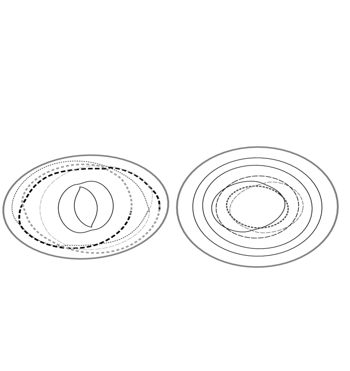
Figure 2: Examples of trajectories of the two component system consisting of $n=6$ unit charges and $m=1$ charge $-\Lambda$, where $\Lambda=1.213579$. Every curve shows an individual trajectory of each charge in its own coordinates $(\Re x_{j},\Im x_{j}),j=1..6$ or $(\Re y_{j},\Im y_{j}),j=1$. The charge of value $-\Lambda$ is depicted by the gray solid line. The motion shown on the left figure has period $4\pi/\omega=2T$, while the period on the right figure is equal to $T=2\pi/\omega$. The motion on the left is depicted within the time interval $t=[0,T]$, which is a half-period for such initial conditions. In this case trajectories of several charges coincide interchanging each half-period $T$.

We devote the rest of this section to examples in favor of this conjecture.

We take the case $\Lambda=1$ as the first example: According to corollary 1 the equations of motion can be reduced to the Lax form (see eg [19])

$$i\frac{d}{dt}L_{x}=[L_{x},A_{x}]+\omega L_{x},\,i\frac{d}{dt}L_{y}=[L_{y},A_{y}]+\omega L_{y}$$

where $L_{y},A_{y}$ and $L_{y},A_{y}$ are matrices of dimensions $n\times n,m\times m$ respectively

$$\begin{array}[]{c}(L_{x})_{jk}=\frac{1}{2}\left(i\frac{dx_{j}}{dt}+\omega x_{j}\right)\delta_{kj}+\frac{1-\delta_{jk}}{x_{j}-x_{k}},\quad j,k\in N\\ \\ (L_{y})_{jk}=\frac{1}{2}\left(i\frac{dy_{j}}{dt}+\omega y_{j}\right)\delta_{kj}+\frac{1-\delta_{jk}}{y_{j}-y_{k}},\quad j,k\in M\end{array}$$ (55)

Substituting (24) to (55) we eliminate velocities $dx/dt,dy/dt$, getting the Lax matrices $\tilde{L_{x}}$ and $\tilde{L_{y}}$ for (24), depending on the coordinates only. It is easy to see that the absolute values of squares of traces

$$I_{1}=({\rm Tr}L)({\rm Tr}L)^{*},\quad I_{2}=({\rm Tr}L^{2})({\rm Tr}L^{2})^{*},..,I_{2(n+m)-1}=({\rm Tr}L^{2(n+m)-1})({\rm Tr}L^{2(n+m)-1})^{*}$$ (56)

of the $(m+n)\times(m+n)$ matrix

$$L=\left(\begin{array}[]{cc}{\tilde{L}_{x}}&0\\ 0&{\tilde{L}_{y}}\end{array}\right)$$

are real rational integrals of motion. They are homogeneous functions in $x,y,\omega$ (with $x,y$ and $\omega$ having weights $-1,-1,2$ respectively). The functional independence of (56) can be easily proven by considering them as polynomials in $\omega$ with functionally independent highest symbols

$$I_{k}=\omega^{2k}\left(\sum_{j\in N}x_{j}^{k}+\sum_{j\in M}y_{j}^{k}\right)\left(\sum_{j\in N}(x^{*}_{j})^{k}+\sum_{j\in M}(y^{*}_{j})^{k}\right)+..,\quad k=1..2(n+m)-1$$

Let us now turn to the general system $\Lambda\not=0,\pm 1$. Although, in this case, our arguments in favor of inetgrability of (52) stem mainly from numerical studies, we would like to mention some analytic results:

The Hamiltonian (54) admits total separation of variables in low dimensions $n+m<4$. Namely, separating motion of the center of mass, we obtain one or two dimensional problem, admitting (in the latter case) further separation of variables in the polar coordinates.

Another (less trivial) example is the system with even number of unit charges $n=2l$ and a single particle of the second type $m=1$ having an arbitrary charge $-\Lambda$. The system is subject to symmetric initial conditions:

$$x_{j}(0)=x_{j+l}(0),\quad y_{1}(0)=0,\quad j=1..l$$

It is seen without much difficulty that due to this ${\mathbb{Z}}_{2}$ symmetry, the above conditions hold for any $t$. Taking this fact into account, we may reduce (52) by this symmetry keeping only variables $x_{j},j=1..l$. Changing the variables as $x_{j}=\sqrt{z_{j}}$ we arrive to the following equations of motion

$$i\frac{dz_{j}}{dt}=-\sum_{k\not=j}\frac{4z_{j}}{z_{j}-z_{k}}+\omega$$ (57)

which corresponds to the ${\rm BC}_{n}$ rational case of figure 1. The integrability of (57) is then provided by arguments used for the study of linear dynamics. The rational integrals of motion for (57) can be found using the Lax representation for the Calogero-Moser system of the ${\rm BC}_{n}$ type.

One can also prove the periodicity of small nonsymmetric deviations from the symmetric trajectories as linear perturbations around (57). We do not perform this analysis here, since it requires cumbersome calculations.

Finally, numerical simulations show that for any initial conditions and real $\Lambda$ trajectories of (52) turn out to be periodic, which shows existence of $2(n+m)-1$ independent rational integrals of motion. The period of motion is an integer multiple the period of the “free” oscillator $T=2\pi/\omega$, with an integer factor depending on the initial conditions.

Typical examples of trajectories for generic initial conditions and $\Lambda$ are shown on figure 2.

IX. Conclusions and Open Questions

The results at which we have now arrived may be summed up as follows: The bilinear hypergeometric operator (1) induces dynamics (2), which may be embedded in a Hamiltonian flow. In the case $\Lambda=1$ this flow is generated by a sum of two independent Calogero(Sutherland)-Moser Hamiltonians (theorem 2) with (generally) different forms of external potentials. This allows us to integrate (24) by the Lax method. The fixed points of the bilinear evolution correspond to equilibrium distributions of different species of point vortices on the plane or cylinder. They may be obtained (again, for $\Lambda=1$) by a finite number of Darboux transformations from the eigenstates of associated linear problems (propositions 4, 5, 7). The dynamical system (52) of two species of interacting points in an external field is conjectured to be completely integrable for arbitrary real $\Lambda$ and $\omega$.

Let us now mention some open questions

The main problem, of course, is to prove integrability of (52) for arbitrary $\Lambda$ (conjecture 1). It might be done by using two approaches: The first approach is to find a Lax representation for (52). The Lax matrices for arbitrary $\Lambda$ could have a complicated structure, being rational functions of $x,y$ and $\omega$ of greater homogeneity degree in comparison with the Calogero-Moser case. It makes hard to find them using straightforward computational approaches.

Another method is to try to linearize (53). Although, as was mentioned before, such a linearisation, connected with the KP equation, was possible for $P=1$ and $\Lambda=1$, we cannot apply a similar scheme in general case.

Another set of questions is connected with solutions of bilinear hypergeometric equation:

In 1929 [7], Burchenall and Chaundy studied the following question: What conditions must be satisfied by two polynomials $p(z),q(z)$ in order that the indefinite integrals

$$\int\left(\frac{p(x)}{q(x)}\right)^{2}dx,\quad\int\left(\frac{q(x)}{p(x)}\right)^{2}dx$$

may be rational, provided $p$ and $q$ do not have multiple and common roots?

They found that the integrals are rational if $p=\theta_{i}$, $q=\theta_{i+1}$ are (now know as the Adler-Moser) polynomials satisfying (43).

From the other hand, we know that any two polynomial solutions of the ordinary hypergeometric equations $p=Q_{n},q=Q_{m}$ are orthogonal with the measure $\nu(z)$

$$\int\nu(z)Q_{n}(z)Q_{m}(z)dz=0,n\not=m$$

Since the two above integrals are related to particular forms of (4), it is natural to ask the following question: what integration condition may be imposed on two polynomials $p$ and $q$ in order for they satisfy a nondegenarate bilinear hypergeometric equation (4)?

In the same work [7], Burcnall and Chaundy have shown that any polynomial solutions of (43) may be obtained by a finite number of Darboux transformation from the kernel of the ”free” differential operator $d^{2}/dz^{2}$.

In this paper we have proved proposition 4, stating that polynomials obtained from the eigenfunctions of the ordinary hypergeometric equation by a finite number of Darboux transformations are solutions of (4). By analogy with [7] it is natural to state the following

Conjecture 2

Any polynomial solutions to bilinear hypergeometric equations of propositions 4, 5 are (38) and (42) respectively.

Concluding the article we would like to mention briefly possible multi-dimensional generalizations of (4). A particular generalization was constructed in section VI for the homogeneous polynomials in two variables (47). A similar construction [5] related to the classical special functions in many dimensions [14], is connected with the quantum Calogero-Moser systems on the Coxeter root systems (and their deformations [6] , [9]). In this context, it would be interesting to find a proper analog of (4) in many dimensions.

Acknowlegements

The author is grateful to H.Aref, F.Calogero, B.Dubrovin, A.Kirillov, A.Orlov for useful information and remarks.

References

[1] M. Adler, J. Moser, On a class of polynomials connected with the
Korteveg-de Vries equation, Comm.Math.Phys. 61 (1978) 1-30
[2] Aref H. Integrable, Chaotic and turbulent motion of vortices in two dimensional flows Ann.Rew.Fluid Mech. 15 345-389 (1983)
[3] Arnold V. I. , Khesin B. A. Topological methods in
hydrodynamics , Springer-Verlag, NY 1998
[4] A. B. Bartman, A new interpretation of the Adler-Moser KdV
polynomials: interaction of vortices, Nonlinear and Turbulent Processes in Physics, Vol.3 (Kiev 1983), 1175-1181,
Harwood Academic Publ., Chur, 1984
[5] Y. Berest Huygens principle and the bispectarl problem , CRM Proceedings and Lecture Notes, Vol. 14, 1998
[6] Y.Berest, I.Loutsenko , Huygens principle in Minkowski
space and soliton solutions of the Korteveg de-Vries equation Comm.Math.Phys, 190 113-132 (1997)
[7] Burcenall J. L. Chaundy T. W. A set of
differential equations which can be solved by polynomials ,
Proc. London Soc, 1929
[8] F.Calogero, Motion of poles and zeros of special solutions of nonlinear
and linear partial differential equations and related ”solvable” many body problems
43 b 177 (1978)
[10] D.Choodnovsky and G.Choodnovsky Pole expansions
of nonlinear partial differential equations, Nuovo Cimento 40 B 339 (1977)
[11] Crum M Associated Sturm-Liouville Systems
Quart.J.Math 6 121-127 (1955)
[12] G.B.Gurevich, Foundations of the Theory of
Algebraic Invariants, Groningen, Holland: P.Noordhoff 1964
[13] Hadamard J. , Lectures on Cauchy’s problem
in linear partial differential equations , Yale Univ. Press,
New Haven, 1923
[14] Heckman G.J., Opdam E.M., Root systems and
hypergeometric functions I. , Composito Math. 64 (1987) 329-352
[15] Inozemtsev V., On the motion of classical
integrable systems of interacting particles in an external field ,
Phys.Lett. 98 316-318 (1984)
[16] I.Krichever Methods of algebraic geometry
in the theory of nonlinear equations Russian Math.Surveys 32,
185-213 (1977)
[17] I.Krichever Rational solutions of the
Kadomtsev-Petviashvili equation and integrable systems of
N particles on line Funct.Anal.Appl., Vol.12, (1978)
[18] Novikov S., Pitaevski L., Zakharov V., Manakov S.,
Theory of solitons: inverse scattering method,
the Contemporary Soviet Mathematics, New York, NY, 1984
[19] A. M. Perelomov Integrable systems in classical
mechanics and Lie’s algebras, Moscow, Nauka, 1990
[20] G. Szegö Orthogonal polynomials, AMS, NY 1939