Regular Spacings of Complex Eigenvalues in the One-dimensional non-Hermitian Anderson Model

Abstract

We prove that in dimension one the non-real eigenvalues of the non-Hermitian Anderson (NHA) model with a selfaveraging potential are regularly spaced. The class of selfaveraging potentials which we introduce in this paper is very wide and in particular includes stationary potentials (with probability one) as well as all quasi-periodic potentials. It should be emphasized that our approach here is much simpler than the one we used before. It allows us a) to investigate the above mentioned spacings, b) to establish certain properties of the integrated density of states of the Hermitian Anderson models with selfaveraging potentials, and c) to obtain (as a by-product) much simpler proofs of our previous results concerned with non-real eigenvalues of the NHA model.

1 Introduction

The non-Hermitian Anderson model (NHA model) was introduced by N. Hatano and D. Nelson in 1996. It arises in the physics of vortex matter, [5, 6], and in many other contexts, see e.g. [4, 11, 12]. This model is described by the following operator

$$(H_{n}^{g}\varphi)_{k}=-e^{g}\varphi_{k+1}+q_{k}\varphi_{k}-e^{-g}\varphi_{k-1},\ \ 1\leq k\leq n$$ (1)

with periodic boundary conditions

$$\varphi_{0}=\varphi_{n},\ \varphi_{1}=\varphi_{n+1}.$$ (2)

Here $g$ is a real parameter, $g\geq 0$. The Hilbert space is $l_{2}(1,n)$ with the standard inner product: if $\varphi=\{\varphi_{j}\}_{j=1}^{n}$ and $\psi=\{\psi_{j}\}_{j=1}^{n}$ are two vectors from $l_{2}(1,n)$, then $(\varphi,\psi)=\sum_{j=1}^{n}\varphi_{j}\bar{\psi}_{j}$.

Hatano and Nelson considered the case when the values $q_{j}$ of the potential are taken as a realization of a sequence of independent identically distributed random variables. By conducting a numerical experiment they discovered a number of remarkable properties both of the spectrum and the eigenfunctions of the operator $H_{n}^{g}$. It turns out that the asymptotic behavior of the eigenvalues depends strongly on the value of the parameter $g$. To demonstrate this statement we present in Fig.1 results of a similar numerical experiment. These pictures are not so well predictable in the following sense. It is a consequence of the Weyl criterion that the spectrum of the limiting random operator ($n=\infty$) contains with probability 1 the union of spectra of operators with constant potentials, $q_{j}\equiv q$, for any real $q$ belonging to the support of the random variable $q_{1}$. A very simple calculation shows then that the spectrum of $H_{\infty}^{g}$ would typically contain (with probability 1) a two-dimensional subset of the complex plain. (A much more detailed description of the spectrum of the limiting operator can be found in [3].) However, numerical experiments reproduce pictures like that in Fig.1 with remarkable stability also for large values of $n$ (in [5, 6] $n=1000$). They clearly show that the eigenvalues of $H_{n}^{g}$ have no tendency to spread over any two-dimensional region but rather tend to belong to smooth curves.

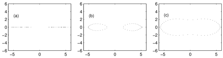
Figure 1: The eigenvalues of $H_{n}^{g}$, are presented by dots plotted in the complex plane. Here $n=50$ and $\{q_{k}\}$ is a fixed realization of independent samples from the uniform distribution on $[-4,-3]\cup[3,4]$; the values of $g$ are: (a) $g=0.2$, (b) $g=1.1$, (c) $g=1.4$.

Our attempt to understand whether this phenomenon would indeed persist as $n\to\infty$ or is due to the fact that $n$ is not large enough stimulated the appearance of two papers [7, 8] where the analysis of the spectra of operators $H_{n}^{g}$ for finite but large values of $n$ was carried out. We shall now briefly describe some of our results restricting ourselves to the case of bounded potentials. Namely it turns out that there are critical values $\underline{\hskip 2.15277ptg}_{\mathrm{cr}}$ and $\bar{g}_{cr}$ depending only on the distribution of the random potential and such that:

1. If $0\leq g<\underline{\hskip 2.15277ptg}_{\mathrm{cr}}$ then the eigenvalues of $H_{n}^{g}$ are “asymptotically” real (see Theorem 3.2 for the exact meaning of this statement). Moreover their limiting distribution does not depend on $g$ and is the same as in the Hermitian case (that is with $g=0$).

2. If $\underline{\hskip 2.15277ptg}_{\mathrm{cr}}<g<\bar{g}_{cr}$ then a finite proportion of eigenvalues moves out of the real axes and places itself on very smooth curves in the complex plane. These curves converge to non-random limiting curves as $n\to\infty$. Moreover we found the limiting density of states for non-real eigenvalues and proved that the “asymptotically” real eigenvalues have the same limiting distribution as in the case of the self-adjoint model.

3. If $g>\bar{g}_{cr}$ then virtually all eigenvalues leave the real axes.

One thus concludes that the phenomenon described above persists as $n$ is growing. The fact that the spectrum of the limiting operator is two-dimensional means that on this spectrum (but off the above mentioned curves) the resolvent of $H_{n}^{g}$ exists but its norm tends to infinity as $n\to\infty$. (See also [14] where the spectrum and the behavior of the norm of the resolvent of random bidiagonal matrices were studied.)

In the present paper we investigate spacings between the neighboring non-real eigenvalues. We do this for models with selfaveraging (deterministic!) potentials which are introduced below. The class of selfaveraging potentials is very wide and includes in particular random stationary, quasi-periodic, and many other potentials.

The approach used in [7, 8] was based on the theory of products of random matrices and on the potential theory. We would like to emphasize that the present paper is self-contained and that the technique we use here is much simpler and more straightforward than that we used before. It allows us:

- To prove that the non-real eigenvalues of NHA model behave in a very regularly way: not only do they belong to very smooth curves as $n\to\infty$ but also the difference between any two neighboring non-real eigenvalues $z_{k+1}$ and $z_{k}$ can be calculated with a great deal of precision as

$$z_{k+1}-z_{k}=\frac{2\pi i}{f(z_{k})}\frac{1}{n},$$

where $f(z)$ is an analytic function of $z$ (Theorem 3.5). This is our principal new result.

- To establish the log-Hölder continuity of the density of states for Hermitian Anderson models with selfaveraging potentials.

- To obtain (essentially as a by-product) much simpler proofs of our previous results listed above.

Remarks. 1. In [7, 8] we considered tri-diagonal matrices with off-diagonal elements $H(j,j+1)$ and $H(j,j-1)$ depending on $j$. All results of this paper can be extended to these models. The main additional condition that is needed is the existence of finite limits $\lim_{n\to\infty}n^{-1}\sum_{j=1}^{n}\ln H(j,j+1)$ and $\lim_{n\to\infty}n^{-1}\sum_{j=2}^{n}\ln H(j,j-1)$.

2. We have already mentioned above that, apart of the fact that stationary potentials provide natural examples of self-averaging potentials, randomness does not play any role in this paper. However as soon as one wishes to understand the real meaning of the next order term in formula (31) randomness becomes crucial. The very same thing applies to the properties of asymptotically real eigenvalues. Namely, it is natural to conjecture that the asymptotically real eigenvalue in fact are real for sufficiently large values of $n$. However there are reasons to believe that in order to prove this conjecture one should restrict himself to the class of random potentials with good properties.

3. The approach based on the theory of products of random matrices (TPRM) is more difficult than that of the present work. However, all main results of this paper can be obtain within the framework of the TPRM. Moreover this is what we did first. The additional advantage of the TPRM approach is that the case of one-dimensional differential Schroedinger operators can be treated by this method in exactly the same way as the discrete case. The attempt to extend the approach of this paper to the case of continuous space would lead to the necessity of using a certain regularization procedure similar to the one used in [2].

The paper is organized as follows. We introduce the class of selfaveraging potentials and discuss the log-Hölder continuity of the relevant density of states in Section 2. Section 3 contains the statement of main results which are proved in Section 4. In Appendix A we prove a version of a well known property of Lyapunov exponents (which we use in Section 2). This allows us to (a) make our exposition even more self-contained and (b) to demonstrate one more application of the technique we use. Appendix B contains an example of calculation of Lyapunov exponents for models whose potentials have rare high peaks. We believe that these examples are of their own interest but the initial purpose of finding them was to provide a natural completion for the study of selfaveraging potentials.

2 The selfaveraging potentials

We introduce now a class of deterministic potentials for which the distribution of the eigenvalues of the NHA model (1) – (2) will be investigated in this paper.

Given an infinite sequence of real numbers $q\equiv\{q_{k}\}_{k=1}^{\infty}$, we consider the sequence of selfadjoint operators $H_{n}^{0}$, $n=2,3,\ldots$, with potential $q$. Let $N_{n}(E)$ be the distribution function of the eigenvalues of $H_{n}^{0}$,

$$N_{n}(E)=\frac{1}{n}\#\{E_{i}\ :\ E_{i}\in\hbox{spectrum of $H_{n}^{0}$ and $E_{i}<E$}\}.$$ (3)

Definition We say that a real potential $q$ is selfaveraging if the integrated density of states of the self-adjoint Anderson model with this potential exists, i.e. there exists a non-decreasing function $N(E)$ such that $N_{n}(E)\longrightarrow N(E)$ as $n\to\infty$ at the points of continuity of $N(E)$.

Remarks: 1. We have borrowed the name ‘selfaveraging’ from the theory of random operators, where it is normally associated with convergence of $N_{n}(E)$ to a nonrandom limiting function.

2. The class of selfaveraging potentials is very wide. For example, it contains decaying potentials, periodic and almost periodic potentials, and stationary random potentials, see e.g. book [10] for proofs and more examples.

3. We do not require $\int dN(E)=1$. However, in many cases (and in particular in those mentioned above) the sequence of measures $dN_{n}(E)$ is tight and hence cannot lose mass.

4. The choice of periodic boundary conditions for $H_{n}^{0}$ is not essential, for example one could use the Dirichlet boundary conditions $\varphi_{0}=\varphi_{n+1}=0$ instead. This is because changing boundary conditions amounts to a rank two perturbation of $H_{n}^{0}$, and hence has no effect on $N(E)$ provided the perturbed finite interval operators remain selfadjoint. Our preference for the periodic boundary conditions will become apparent in the next section.

Let

$$U_{n}(x,y)\overset{\rm def}{=}\int_{-\infty}^{+\infty}\ln|x+iy-E|dN_{n}(E)\equiv\frac{1}{n}\sum_{j=1}^{n}\ln|x+iy-E_{j}|,$$ (4)

where the summation is over all eigenvalues of $H_{n}^{0}$, and

$$U(x,y)\overset{\rm def}{=}\int_{-\infty}^{+\infty}\ln|x+iy-E|dN(E),\hskip 12.91663ptx,y\in\mathbb{R},$$ (5)

Obviously the logarithmic integrals $U(x,y)$ and $U_{n}(x,y)$ are the real parts of the analytic functions

$$F(z)\overset{\rm def}{=}\int_{-\infty}^{+\infty}\ln(E-z)dN(E)=U(x,y)+iV(x,y).$$ (6)

$$F_{n}(z)\overset{\rm def}{=}\int_{-\infty}^{+\infty}\ln(E-z)dN_{n}(E)=U_{n}(x,y)+iV_{n}(x,y).$$ (7)

Here and below we consider analytic functions defined in the upper half-plane $\mathbb{C}_{+}=\{z\in\mathbb{C}:\hskip 4.30554pt\mathop{\mathrm{Im}}z>0\}$, and the branch of the $\ln(E-z)$ is chosen so that $\ln(-i)=-i\frac{\pi}{2}$.

The functions defined in (4) – (7) play an important role in this paper. In this section we study their properties under the following conditions

• The potential $q$ is selfaveraging.

• $\sup_{n\geq 1}\frac{1}{n}\sum_{k=1}^{n}\ln(1+|q_{k}|)\leq C<+\infty$.

The main role of Condition C2 is to ensure that the functions $U(x,y)$ and $F(z)$ are well defined:

Proposition 2.1

Assume C1-C2. Then for every $x,y\in\mathbb{R}$ the integral in (5) is converging.

Proof. Suppose first that $y>0$ and let $z=x+iy$. Note that

$$\ln y\leq U_{n}(x,y)\leq\ln(2+|z|)+C\hskip 12.91663pt\hbox{for all $x\in\mathbb{R}$ and $y>0$.}$$ (8)

The LHS inequality is trivial, and the RHS inequality is ensured by Condition C2. Indeed,

$$U_{n}(x,y)\leq\frac{1}{n}\sum_{j=1}^{n}\ln(2+|z|+|q_{j}|),$$

where the last inequality follows, e.g., from the representation $U_{n}(x,y)=\frac{1}{n}\ln|\det(zI_{n}-H_{n}^{0})|$ and Hadamard’s inequality for the determinants. By Condition C2,

$$\frac{1}{n}\sum_{j=1}^{n}\ln(2+|z|+|q_{j}|)\leq\ln(2+|z|)+C.$$

If $A>-\infty$ and $B<+\infty$ are points of continuity of $N(E)$ then, in view of Condition C1,

$$\int_{A}^{B}\ln|z-E|dN(E)=\lim_{n\to\infty}\int_{A}^{B}\ln|z-E|dN_{n}(E) \leq \lim_{n\to\infty}\int_{A}^{B}\ln|z+i-E|dN_{n}(E)$$

$$\leq \limsup_{n\to\infty}U_{n}(x,y+1).$$

Applying (8), we obtain that

$$\int_{A}^{B}\ln|z-E|dN(E)\leq\ln(3+|z|)+C.$$ (9)

As $y\not=0$, the function $\ln|z-E|$ is bounded from below, and (9) implies that the integral in (5) is converging for $y>0$. By the symmetry, it is also converging for $y<0$.

We shall now make use of the following inequality which will be proved later (Theorem 2.6): $U(x,y)\geq-c_{0}$ for some $c_{0}>0$ and all $x$ and $y\not=0$. This inequality together with the monotone convergence theorem yield that

$$\lim_{y\downarrow 0}U(x,y)=\int_{-\infty}^{+\infty}\ln|x-E|dN(E)\geq-c_{0},$$ (10)

hence the integral in (5) is also converging for $y=0$. $\Box$

Remark. It follows from (10) that $N(\cdot)$ is a continuous function. Therefore, under Conditions C1 and C2, we have that $N_{n}(E)$ converges pointwise to $N(E)$ as $n\to\infty$, and the convergence is uniform in $E,\ -\infty<E<\infty$.

In view of the inequalities

$$Q_{n}-2\leq H_{n}^{0}\leq Q_{n}+2$$ (11)

where $Q_{n}$ is the operator of multiplication by $q$, $(Q_{n}\varphi)_{j}=q_{j}\varphi_{j}$, $j=1,\ldots,n$, Condition C2 also ensures that the sequence of measures $dN_{n}(E)$ is tight:

Proposition 2.2

Suppose that $q$ satisfies Condition C2. Then for any $\varepsilon>0$ there exists $B>0$ such that $N_{n}(B)-N_{n}(-B)>1-\varepsilon$ for all $n$.

Proof. Denote by $\chi_{B}(E)$ the indicator-function of the interval $[B,+\infty)$, and let $E_{1},\ldots,E_{n}$ be the eigenvalues of $H_{n}^{0}$. Then for any $B>0$

$$1-N_{n}(B)=\frac{1}{n}\sum_{j=1}^{n}\chi_{B}(E_{j})\leq\frac{1}{n}\sum_{j=1}^{n}\chi_{B}(E_{j})\frac{\ln(1+E_{j})}{\ln(1+B)}\leq\frac{1}{n}\sum_{j=1}^{n}\chi_{B}(2+q_{j})\frac{\ln(1+2+q_{j})}{\ln(1+B)}$$

where the last inequality follows from (11). We use here the following fact: if $f(E)$ is a non-decreasing function and $A\leq B$ then $\mathop{\mathrm{tr}}f(A)\leq\mathop{\mathrm{tr}}f(B)$. Since $\chi_{B}(2+q_{j})\ln(1+2+q_{j})\leq\ln(1+|2+q_{j}|)$ we conclude, in view of Condition C2, that $N_{n}(B)\geq 1-C^{{}^{\prime}}/\ln(1+B)$ for some constant $C^{{}^{\prime}}>0$ and all $n$. Similarly, $N_{n}(-B)\leq C^{{}^{\prime\prime}}/\ln(1+B)$ for some constant $C^{{}^{\prime\prime}}>0$ and all $n$. $\Box$

We shall now investigate the relation between $F_{n}(z)$ and $F(z)$ in the limit $n\to\infty$.

Proposition 2.3

Assume C1-C2. Then for every real $x$ and $y\not=0$

$$\liminf_{n\to\infty}U_{n}(x,y)\geq U(x,y).$$ (12)

Proof. For all $B$ large enough (so that $[x-1,x+1]\subseteq[-B,B]$) we have that for any $n$

$$U_{n}(x,y)\geq\int_{-B}^{B}\ln|x+iy-E|dN_{n}(E)$$

and, by Condition C1,

$$\liminf_{n\to\infty}U_{n}(x,y)\geq\int_{-B}^{B}\ln|x+iy-E|dN(E).$$

By letting $B\to\infty$, we obtain (12). $\Box$

Under Conditions C1 and C2, the sequence $\{U_{n}(x,y)\}$ is not necessarily converging, even for $y\not=0$, and for some selfaveraging potentials the inequality in (12) is strict, for examples see Appendix B.

In view of (8), for any compact set $K\subset\mathbb{C}_{+}$, $\sup_{K}|F_{n}(z)|\leq M(K)$ for some constant $M(K)<+\infty$ and all $n$. Hence the sequence $\{F_{n}(z)\}$ has a uniformly converging subsequence. We shall now describe all limit points of $\{F_{n}(z)\}$:

Theorem 2.4

Assume C1-C2. Suppose that $F_{n_{j}}(z)$ is a converging subsequence of $\{F_{n}(z)\}$. Then necessarily

$$\lim_{j\to\infty}F_{n_{j}}(z)=F(z)+c$$ (13)

for all $z\in\mathbb{C}_{+}$ and some real constant $c$ satisfying the inequality $0\leq c\leq\ln 3+C$, where $C$ is the constant defined in Condition C2.

Proof. We note that $F^{{}^{\prime}}_{n}(z)=\int_{-\infty}^{+\infty}(z-E)^{-1}dN_{n}(E)$ and $F^{{}^{\prime}}(z)=\int_{-\infty}^{+\infty}(z-E)^{-1}dN(E)$. Since the function $h(E)=(z-E)^{-1}$ decays to zero at infinity, Condition C1 ensures that

$$\lim_{n\to\infty}F^{{}^{\prime}}_{n}(z)=F^{{}^{\prime}}(z)$$

uniformly in $z$ on compact sets in $\mathbb{C}_{+}$. Therefore there exists a sequence of complex constants $c_{n}$ such that $F_{n}(z)-c_{n}\longrightarrow F(z)$ as $n\to\infty$ for all $z\in\mathbb{C}_{+}$. Passing on to the converging subsequence $F_{n_{j}}(z)$, we have that $c_{n_{j}}$ is also converging. Putting $c=\lim_{j}c_{n_{j}}$ we arrive at (13). It remains to prove that $c$ is real, non-negative and satisfies the inequality $c\leq\ln 3+C$.

Due to our choice of the branch of the log-function we have that $-\pi\leq\mathop{\mathrm{Im}}\ln(E-z)\leq 0$ for all $z\in\mathbb{C}_{+}$. Thus

$$\mathop{\mathrm{Im}}F_{n}(z)=\int\mathop{\mathrm{Im}}\ln(E-z)dN_{n}(E)\longrightarrow\mathop{\mathrm{Im}}F(z),\hskip 12.91663pt\hbox{as $n\to\infty$},$$

because the integrand is bounded, the sequence of measures $dN_{n}(E)$ is tight and we have Condition C1. Therefore the constant $c$ is real. The fact that it is non-negative follows from Proposition 2.3. To complete the proof, note that $U_{n_{j}}(x,y)$ converges to $U(x,y)+c$ in the upper half of the $xy$-plane. Therefore, because of (8), $U(x,y)+c\leq\ln(2+|z|)+C$. Putting here $x=0$ and $y=1$, we obtain $c\leq\ln 3+c-U(0,1)\leq\ln 3+C$. (Obviously, $U(x,1)\geq 0$ for all $x$.) $\Box$

The following condition

• for any $\varepsilon>0$ there is a $B>0$ such that $\frac{1}{n}\sum\limits_{j=1}^{n}\chi_{B}(|q_{j}|)\ln(1+|q_{j}|)<\varepsilon$ for all $n$

guarantees the convergence of $F_{n}(z)$ to $F(z)$. It is obvious that Condition C2* is somewhat more restrictive than C2. On the other hand it is satisfied by many popular classes of potentials. For example, the random stationary potentials with finite expectation of $\ln(1+|q_{j})$ satisfy Condition C2* with probability one. It is also satisfied if

$$\frac{1}{n}\sum_{j=1}^{n}\ln^{1+\delta}(1+|q_{j}|)\leq C^{*}<+\infty\hskip 12.91663pt\hbox{for some $\delta>0$.}$$

Proposition 2.5

Assume C1 and C2*. Then

$$F_{n}(z)\underset{n\to\infty}{\longrightarrow}F(z)\hskip 8.61108pt\hbox{uniformly in $z$ on compact sets in $\mathbb{C}_{+}$}$$ (14)

and, in particular,

$$U_{n}(x,y)\underset{n\to\infty}{\longrightarrow}U(x,y)\hskip 8.61108pt\hbox{uniformly in $z=x+iy$ on compact sets in $\mathbb{C}_{+}$}.$$ (15)

Proof. If the potential $q$ is bounded then the statement of Proposition 2.5 is a straightforward corollary of Condition C1 and the fact that the functions $F_{n}(z)$ are equicontinuous on any compact subset of $\mathbb{C}_{+}$. If $q$ is unbounded then one needs to show additionally that the contribution of the tails of $dN_{n}(E)$ to $F_{n}(z)$ is negligible in the limit $n\to\infty$. Obviously, it will suffice to prove that:

$$\hbox{for any $\varepsilon>0$ there is a $B>0$ such that $\frac{1}{n}\sum\limits_{k=1}^{n}\chi_{B}(|E_{k}|)\ln(1+|E_{k}|)<\varepsilon$ for all n},$$ (16)

where the summation in (16) is effectively over all eigenvalues of $H_{n}^{0}$ such that $|E_{j}|\geq B$. To complete the proof note that, in view of the inequalities in (11), it is apparent that Condition C2* implies (16). $\Box$

We finish this Section with a proof of the log-Hölder continuity of $N(E)$. This property is well known for random potentials and in this case it follows from the fact that $U(x,y)\geq 0$ [2]. In turn, this inequality is a consequence of the Thouless formula according to which $U(x,y)$ coincides with the Lyapunov exponent of $H_{n}^{0}$ with $n=\infty$, see e.g. [2, 10, 1].

In our case Conditions C1 and C2 are too weak to guarantee the existence of the Lyapunov exponent even for non-real values of the spectral parameter, see examples in Appendix B. However these two conditions ensure that the function $U(x,y)$ is bounded from below which, in turn, implies (very much in the same ways as in [2]) that $N(E)$ is log-Hölder continuous.

Theorem 2.6

Assume C1-C2. Then:

• $U(x,y)\geq-c_{0}$ for some $c_{0}>0$ and all real $x$ and $y$.

• $N(E)$ is log-Hölder continuous: for any $E$ and $|\sigma|\leq\frac{1}{2}$

  $$|N(E+\sigma)-N(E)|=c(E,\sigma)|\ln|\sigma||^{-1}\ \hbox{ where }\ \lim_{\sigma\to 0}c(E,\sigma)=0.$$ (17)

  If $E$ belongs to a compact set then $c(E,\sigma)\leq c_{1}$ with the constant $c_{1}$ depending only on this compact set and the constant $C$ in Condition C2.

Proof. Part (i). In view of (10) and the symmetry in $y$, it will suffice to prove the inequality for $y>0$ only. It follows from Theorem 2.4 that

$$\liminf_{n\to\infty}U_{n}(x,y)=U(x,y)+c_{0}$$ (18)

for some $c_{0}\geq 0$ and all $x$ and $y\not=0$. To finish the proof, it is sufficient to show that the LHS in (18) is non-negative. If the $\lim_{n\to\infty}U_{n}(x,y)$ exists then it coincides with the Lyapunov exponent, and hence is non-negative. The general case can be treated similarly (see Appendix A).

Part (ii). Since $\int\ln|x-E|dN(E)\geq-c_{0}$, we have that

$$\int_{|x-E|\leq 1}\ln|x-E|\,dN(E)+\int_{|x-E|>1}\ln|x-E|\,dN(E)\geq-c_{0},$$

and

$$\int\limits_{|x-E|\leq 1}\ln\frac{1}{|x-E|}\,dN(E)\leq\int\limits_{|x-E|>1}\ln|x-E|\,dN(E)+c_{0}\leq U(x,1)+c_{0}.$$

Therefore, for any $|\delta|\leq\frac{1}{2}$,

$$U(x,1)+c_{0}\geq\int\limits_{|x-E|\leq|\delta|}\ln\frac{1}{|x-E|}\,dN(E)\geq|N(x+\delta)-N(x-\delta)|\ln\frac{1}{|\delta|},$$

and

$$|N(x+\delta)-N(x-\delta)|\leq[U(x,1)+c_{0}]|\ln|\delta||^{-1}.$$ (19)

Note that for any compact set $K\subset\mathbb{R}$, $\max_{K}U(x,1)<+\infty$. This is because $U(x,1)$ is continuous in $x$.

Now, define for $|\delta|\leq\frac{1}{2}$

$$c(x,\delta)=\int_{x}^{x+\delta}\ln\frac{1}{|x-E|}\,dN(E).$$

Obviously,

$$|N(x+\delta)-N(x)|\leq\frac{c(x,\delta)}{|\ln|\delta||}.$$

To complete the proof, note that (19) implies that the measure $dN(E)$ has no atoms, and therefore

$$c(x,\delta)\longrightarrow 0\hskip 8.61108pt\hbox{when $\delta\to 0$.}$$

$\Box$

3 Main results

For the sake of convenience and clarity of exposition, we shall formulate and prove our results for the class of potentials $q$ satisfying Conditions C1 and C2*. We emphasize however that our main results hold true, modulo trivial modifications, under Conditions C1 and C2, and the corresponding proofs are identical to those given in Section 4. This is a mere reflection of Theorem 2.4 and the fact that our proofs are based on the convergence of $F_{n}(z)$ to $F(z)$.

3.1 Notations and auxiliary statements

Let us fix any finite interval $[a,b]$ of the real axis $(a<b)$. Most of our results apply to the part of the spectrum of $H_{n}^{g}$ belonging to the strip $\{z:\ \mathop{\mathrm{Re}}z\in[a,b]\}$ in the complex plane $\mathbb{C}$.

We define several critical values of the parameter $g$:

$$\underline{\hskip 2.15277ptg}_{\mathrm{cr}}=\inf_{x\in\mathcal{S}}U(x,0),\hskip 12.91663pt\bar{g}_{\mathrm{cr}}=\sup_{x\in\mathcal{S}}U(x,0).$$ (20)

where we have introduced the notation $\mathcal{S}$ for the support of the measure $dN(E)$, and

$$\underline{\hskip 2.15277ptg}_{\mathrm{cr}}(a,b)=\inf_{x\in\mathcal{S}\cap[a,b]}U(x,0),\hskip 12.91663pt\bar{g}_{\mathrm{cr}}(a,b)=\sup_{x\in\mathcal{S}\cap[a,b]}U(x,0).$$ (21)

It may happen that $\bar{g}_{\mathrm{cr}}=+\infty$, and it is obvious, in view of Theorem 2.6, that $\underline{\hskip 2.15277ptg}_{\mathrm{cr}}\geq 0$ for any potential satisfying Conditions C1 and C2.

For every $g\in\mathbb{R}$, define

$$\Lambda_{g}=\{x\in\mathbb{R}:\hskip 4.30554ptU(x,0)<g\}.$$ (22)

If $g\leq\underline{\hskip 2.15277ptg}_{\mathrm{cr}}$ then $\Lambda_{g}=\emptyset$, otherwise $\Lambda_{g}$ consists of (possibly infinitely many) disjoint open intervals:

$$\Lambda_{g}=\bigcup_{j}\,(a_{j},b_{j}).$$ (23)

We note also that $U(x,y)=U(x,-y)$ and that

$$\frac{\partial}{\partial y}\,U(x,y)>0\hskip 8.61108pt\hbox{for any}\hskip 4.30554ptx\in\mathbb{R},\hskip 4.30554pty>0.$$ (24)

Proposition 3.1

Suppose that $g>\underline{\hskip 2.15277ptg}_{\mathrm{cr}}$ and let $(a_{j},b_{j})$ be the intervals defined in (23). Then the level set ${\cal L}_{g}=\{(x,y):\hskip 4.30554ptU(x,y)=g,\hskip 4.30554pty>0\}$ consists of disjoint analytic arcs

$$y=y_{j}(x),\hskip 8.61108pta_{j}<x<b_{j},$$ (25)

whose end-points lie on the real axis, i.e. $y_{j}(a_{j}+0)=y_{j}(b_{j}-0)=0$, if $-\infty<a_{j},b_{j}<+\infty$.

Proof. If $x_{0}\notin\Lambda_{g}$ then $U(x_{0},y)>g$ for all $y\not=0$. Therefore the equation $U(x_{0},y)=g$ cannot be solved for $y>0$.

Consider now any of the intervals $(a_{j},b_{j})$. If $x_{0}\in(a_{j},b_{j})$ then $U(x_{0},0)<g$, and in view of (24) and $U(x,+\infty)=+\infty$, there exists a unique positive solution $y_{0}\overset{\rm def}{=}y_{j}(x_{0})>0$ of the equation $U(x_{0},y)=g$. As $U(x,y)$ can be analytically continued into a neighborhood of $(x_{0},y_{0})$ in $\mathbb{C}^{2}$, the implicit function theorem asserts that $y_{j}(x)$ is analytic in a disk $|x-x_{0}|<\delta$ in the complex $x$-plane. The union of all such disks, when $x_{0}$ runs through $(a_{j},b_{j})$ covers $(a_{j},b_{j})$. Therefore the function $y_{j}(x)$ can be analytically continued into a domain in the complex $x$-plane that contains $(a_{j},b_{j})$, and, for any closed interval $[\alpha,\beta]\subset(a_{j},b_{j})$, this domain contains

$$D_{\alpha,\beta}=\{x\in\mathbb{C}:\hskip 4.30554pt\alpha-h\leq\mathop{\mathrm{Re}}x\leq\beta+h,\hskip 4.30554pt|\mathop{\mathrm{Im}}x|\leq h\}$$ (26)

for some $h>0$.

If $a_{j}>-\infty$ then $y_{j}(a_{j}+0)=0$. For, if not then $\bar{y}:=\limsup_{x\to a_{j},x>a_{j}}y_{j}(x)>0$. But then $U(a_{j},\bar{y})=g$ and hence $U(x,0)<g$ for every $x$ from some neighborhood of $a_{j}$ which contradicts the definition of $a_{j}$ as the end point of our interval. The same argument proves that if $b_{j}<+\infty$ then $y_{j}(b_{j}-0)=0$. $\Box$

3.2 Statement of results

We are now in a position to formulate our main results.

Theorem 3.2

For any $g>0$ all the eigenvalues of $H_{n}^{g}$ belong to the level lines of the function $U_{n}(x,y)$ defined by the equation

$$U_{n}(x,y)=g+\frac{2}{n}\ln(1-e^{-ng}).$$ (27)

Theorem 3.3

(i) Suppose that $g\leq\underline{\hskip 2.15277ptg}_{\mathrm{cr}}(a,b)$. Then for any $\varepsilon>0$ there exists $n_{0}=n_{0}(\varepsilon,g,q,a,b)$ such that for any $n>n_{0}$ all the eigenvalues $z_{j}$ of $H_{n}^{g}$ with $\mathop{\mathrm{Re}}z_{j}\in[a,b]$ belong to the $\varepsilon$-neighborhood of the real axis: $|\mathop{\mathrm{Im}}z_{j}|\leq\varepsilon$.

(ii) Suppose that $g>\underline{\hskip 2.15277ptg}_{\mathrm{cr}}$ and $(a_{j},b_{j})$ is one of the intervals comprising $\Lambda_{g}$. Then for any $[\alpha,\beta]\subset(a_{j},b_{j})$ there exists $n_{1}=n_{1}(q,g,\alpha,\beta)$ such that for any $n>n_{1}$ there exists a solution $y_{j,n}(x)$ to equation (27) which is analytic in the domain $D_{\alpha,\beta}$ defined in (26) and

$$\lim_{n\to\infty}y_{j,n}(x)=y_{j}(x),\hskip 12.91663pt\hbox{uniformly in $x\in D_{\alpha,\beta}$}.$$ (28)

The function $y_{j,n}(x)$, for $n>n_{1}$, is the only solution of (27) which is non-negative when $x\in[\alpha,\beta]$.

Remarks. 1. The previous two theorems imply that if $H_{n}^{g}$ has eigenvalues in the strip $a_{j}<\alpha\leq\mathop{\mathrm{Re}}z\leq\beta<b_{j}$, then, for $n>n_{1}$, they must lie on the analytic arc

$${\cal A}_{n}(\alpha,\beta)=\{(x,y):\hskip 4.30554pty=y_{j,n}(x),\hskip 2.15277pt\alpha\leq x\leq\beta\}$$

and on its reflection with respect to the real axis.

2. Relation (28) implies that the arcs ${\cal A}_{n}(\alpha,\beta)$ converge to the level lines of $U(x,y)$ when $n\to\infty$ together with all their derivatives.

3. We did not make use of two out of the four critical values introduced in (20) and (21). However, their role is clear: if $g>\bar{g}_{\mathrm{cr}}(a,b)$ then no limiting eigenvalue curves grow out of the support of $\mathcal{S}\cap[a,b]$. If $\bar{g}_{\mathrm{cr}}$ is finite then $[a,b]$ can be replaced in this statement by $\mathcal{S}$.

The next two theorems describe the asymptotic distribution of the eigenvalues of $H_{n}^{g}$ along the arc ${\cal A}_{n}(\alpha,\beta)$. In particular they state that $H_{n}^{g}$, for large $n$, does have eigenvalues on ${\cal A}_{n}(\alpha,\beta)$.

By $\nu_{n}(\alpha,\beta)$ we denote the number of complex eigenvalues of $H_{n}^{g}$ lying on ${\cal A}_{n}(\alpha,\beta)$.

Theorem 3.4

For any closed interval $[\alpha,\beta]\subset(a_{j},b_{j})$,

$$\lim_{n\to\infty}\frac{1}{n}\nu_{n}(\alpha,\beta)=\frac{1}{2\pi}[\theta(\beta)-\theta(\alpha)],$$

where $\theta(x)=-V(x,y_{j}(x))$ and $V(x,y)$ is the imaginary part of $F(z)$.

Remark. Let $l$ be the natural parameter on the curve $y=y_{j}(x)$, that is the length of the part of this curve contained between say $(\alpha,y_{j}(\alpha))$ and $(x,y_{j}(x))$. A simple calculation involving the Cauchy-Riemann equations for $F(z)$ shows that $d\theta=|f(z(l)|dl$, where

$$f(z)=F^{{}^{\prime}}(z)=\int\frac{dN(E)}{z-E}.$$ (29)

Hence

$$\lim_{n\to\infty}\frac{1}{n}\nu_{n}(\alpha,\beta)=\frac{1}{2\pi}\int_{\alpha}^{\beta}\theta^{\prime}(x)dx=\frac{1}{2\pi}\int_{\alpha+iy_{j}(\alpha)}^{\beta+iy_{j}(\beta)}|f(z(l))|dl,$$ (30)

where the integration is carried out along the path $y=y_{j}(x)$ from $\alpha+iy_{j}(\alpha)$ to $\beta+iy_{j}(\beta)$.

Theorems 3.3 and 3.4 are not entirely new and can be inferred from Theorems 2.1 and 2.2 in [8]. We are now going to formulate our principal new result. Let $[\alpha,\beta]$ be the same as before. Let us label the eigenvalues $z_{k}=x_{k}+iy_{k}$ of $H_{n}^{g}$ lying on the arc ${\cal A}_{n}(\alpha,\beta)$ so that $\alpha\leq x_{1}\leq x_{2}\ldots\leq x_{m}\leq\beta$ (we note that in fact the multiplicity of these eigenvalues is one and the inequalities here are strict; this follows from the inequality $\theta_{n}^{{}^{\prime}}(x)\geq C_{0}>0$ which is a part of the proof of Theorem 3.4).

Theorem 3.5

For any two consecutive eigenvalues $z_{k}$ and $z_{k+1}$ of $H_{n}^{g}$ lying on ${\cal A}_{n}(\alpha,\beta)$,

$$n(z_{k+1}-z_{k})=\frac{2\pi i}{f(z_{k})}+\delta_{n}(z_{k},z_{k+1})$$ (31)

where

$$\lim_{n\to\infty}\delta_{n}(z_{k},z_{k+1})=0\hskip 12.91663pt\hbox{uniformly in}\hskip 4.30554ptz_{k},z_{k+1}\in{\cal A}_{n}(\alpha,\beta).$$ (32)

4 Proofs

The eigenvalues and eigenfunctions of $H_{n}^{g}$ are determined by the equation

$$-e^{g}\varphi_{k+1}+q_{k}\varphi_{k}-e^{-g}\varphi_{k-1}=z\varphi_{k},\ \ 1\leq k\leq n$$ (33)

were

$$\varphi_{0}=\varphi_{n},\ \varphi_{1}=\varphi_{n+1}.$$ (34)

The parameter $g$ can be eliminated from (33) by making use of the standard substitution $\varphi_{k}=e^{-kg}\psi_{k}$ which transforms (33) into

$$-\psi_{k+1}+q_{k}\psi_{k}-\psi_{k-1}=z\psi_{k},\ \ 1\leq k\leq n,$$ (35)

and boundary conditions (34) into

$$\psi_{0}=e^{-ng}\psi_{n},\ \psi_{1}=e^{-ng}\psi_{n+1}.$$ (36)

Note that the transformed boundary conditions are asymmetric (unless $g=0$).

To solve equation (35) we shall follow the standard routine and rewrite it in the matrix form:

$$\left(\begin{array}[]{l}\psi_{k+1}\\ \psi_{k}\\ \end{array}\right)=A_{k}\left(\begin{array}[]{l}\psi_{k}\\ \psi_{k-1}\\ \end{array}\right),\ 0\leq k\leq n,\hskip 4.30554pt\hbox{ where }\ A_{k}=\begin{pmatrix}q_{k}-z&-1\\ 1&0\\ \end{pmatrix}.$$

Then

$$\begin{pmatrix}\psi_{n+1}\\ \psi_{n}\\ \end{pmatrix}=S_{n}(z)\begin{pmatrix}\psi_{1}\\ \psi_{0}\\ \end{pmatrix},\ \hbox{ where }\ S_{n}(z)=A_{n}A_{n-1}\ldots A_{1}.$$

On the other hand,

$$\begin{pmatrix}\psi_{n+1}\\ \psi_{n}\\ \end{pmatrix}=e^{ng}\begin{pmatrix}\psi_{1}\\ \psi_{0}\\ \end{pmatrix}$$

because of boundary conditions (36). Therefore the eigenvalues of $H_{n}^{g}$ are determined by the equation

$$\det[S_{n}(z)-e^{ng}I]=0.$$ (37)

Since $\det S_{n}(z)=1$ for all $z$, we have that

$$\det[S_{n}(z)-e^{ng}I]=1-e^{ng}\mathop{\mathrm{tr}}S_{n}(z)+e^{2ng}.$$

Hence:

Lemma 4.1

$z$ is an eigenvalue of $H_{n}^{g}$ iff

$$\mathop{\mathrm{tr}}S_{n}(z)=e^{ng}+e^{-ng}.$$

The trace of the matrix $S_{n}(z)$ is a polynomial in $z$ of degree $n$. The following representation of this polynomial, which is well known in the context of the discrete Hill equation (see e.g. [13] or [9]) is useful for our purposes.

Lemma 4.2

Let $E_{j}$, $j=1,\ldots,n$, be the eigenvalues of $H_{n}^{0}$. Then

$$\mathop{\mathrm{tr}}S_{n}(z)=\prod_{j=1}^{n}(E_{j}-z)+2.$$ (38)

Proof. For $g=0$, Lemma 4.1 asserts that the polynomials $\prod_{j=1}^{n}(E_{j}-z)$ and $\mathop{\mathrm{tr}}S_{n}(z)-2$ have the same set of zeros. It is easy to verify both polynomials have the same coefficient, $(-1)^{n}$, in front of the highest power of $z$, hence they must coincide. $\Box$

Here is our main technical lemma:

Lemma 4.3

Suppose that $g>0$. Then $z$ is an eigenvalue of $H_{n}^{g}$ iff

$$F_{n}(z)=\frac{2}{n}\ln\Big{(}e^{\frac{ng}{2}}-e^{\frac{-ng}{2}}\Big{)}+\frac{i\pi}{n}\hskip 21.52771pt\Big{(}\mod\frac{2\pi i}{n}\Big{)}$$ (39)

where $F_{n}(z)$ is the function defined in (7).

Proof. It follows from Lemmas 4.1 and 4.2 that $z$ is an eigenvalue of $H_{n}^{g}$ iff

$$\prod_{j=1}^{n}(E_{j}-z)=-(e^{\frac{ng}{2}}-e^{\frac{-ng}{2}})^{2}.$$ (40)

Since $F_{n}(z)=\frac{1}{n}\sum_{j=1}^{n}\ln(E_{j}-z)$, equation (40) is equivalent to (39), provided $g\not=0$. $\Box$

We are now in a position to prove Theorems 3.2 and 3.3.

Proof of Theorem 3.2: This theorem is a straightforward corollary of Lemma 4.3.

Proof of Theorem 3.3: (i) Let $g(\varepsilon)=\min_{x\in[a,b]}U(x,\varepsilon)$. According to Proposition 2.5 one can find $n_{0}$ such that for all $x\in[a,b]$

$$|U_{n}(x,\varepsilon)-U(x,\varepsilon)|\leq\frac{1}{2}[g(\varepsilon)-\underline{\hskip 2.15277ptg}_{\mathrm{cr}}(a,b)]$$

if $n>n_{0}$. (Note that $g(\varepsilon)>\underline{\hskip 2.15277ptg}_{\mathrm{cr}}(a,b)$ because of (24).) Thus, for all $a\leq x\leq b$ and $y\geq\varepsilon$,

$$U_{n}(x,y)\geq U_{n}(x,\varepsilon)\geq U(x,\varepsilon)-\frac{1}{2}[g(\varepsilon)-\underline{\hskip 2.15277ptg}_{\mathrm{cr}}(a,b)]\geq\frac{1}{2}U(x,\varepsilon)+\frac{1}{2}\underline{\hskip 2.15277ptg}_{\mathrm{cr}}(a,b)\geq\underline{\hskip 2.15277ptg}_{\mathrm{cr}}(a,b).$$

Recall that by the assumption $\underline{\hskip 2.15277ptg}_{\mathrm{cr}}(a,b)\geq g$. Since $g>g+\frac{2}{n}\ln(1-e^{-ng})$ for any $n>0$, we conclude that, for all $n>n_{0}$ equation (27) has no solutions in the half-strip $a\leq x\leq b$, $y\geq\varepsilon$. To complete the proof remember that $U_{n}(x,-y)=U_{n}(x,y)$.

(ii) First, note that for every real $x$ equation (27) has one non-negative solution at most.

Now, let $g>\underline{\hskip 2.15277ptg}_{\mathrm{cr}}$ and $[\alpha,\beta]\subset(a_{j},b_{j})$ where $(a_{j},b_{j})$ is one of the intervals comprising $\Lambda_{g}$. Recall that $y_{j}(x)$ is analytic in $D_{\alpha,\beta}$, see Proposition 3.1. Because of the compactness of $[\alpha,\beta]$, it will suffice to prove the existence of the solution $y_{j,n}(x)$ to equation (27) and its convergence to $y_{j}(x)$ as $n\to\infty$ in a small neighborhood of every point $(x,y_{j}(x))$ where $x$ runs through $[\alpha,\beta]$.

Fix $\tilde{x}\in[\alpha,\beta]$ and consider the point $(\tilde{x},\tilde{y})$ where $\tilde{y}=y_{j}(\tilde{x})$. It follows from the integral representations for $U_{n}(x,y)$ and $U(x,y)$ that these two functions are analytic in the domain

$$\tilde{D}\overset{\rm def}{=}\{(x,y):\hskip 4.30554pt|x-\tilde{x}|<\frac{\tilde{y}}{2},\hskip 2.15277pt|y-\tilde{y}|<\frac{\tilde{y}}{2}\}.$$

We shall use the following general lemma. Put $D_{r}\overset{\rm def}{=}\{(x,y):\hskip 4.30554pt|x-\tilde{x}|<r,\hskip 2.15277pt|y-\tilde{y}|<r\}$.

Lemma 4.4

Let $\Phi(x,y)$ and $\tilde{\Phi}(x,y)$ be two functions analytic in $D_{r}$ and such that for all $(x,y)\in D_{r}$

$$|\Phi_{x}^{{}^{\prime}}(x,y)|\leq c_{1},\hskip 4.30554pt0<c_{2}\leq|\Phi_{y}^{{}^{\prime}}(x,y)|\leq c_{3},\hskip 4.30554pt|\tilde{\Phi}(x,y)|\leq 1.$$

Suppose that $\Phi(\tilde{x},\tilde{y})=0$. Then there is a positive $\varepsilon_{0}$ which depends only on $c_{1},c_{2},c_{3},$ and $r$ (but not on $\Phi(\cdot,\cdot)$, $\tilde{\Phi}(\cdot,\cdot)$!) such that the equation

$$\Phi(x,y)+\varepsilon\tilde{\Phi}(x,y)=0$$ (41)

has a unique solution $y=y(x,\varepsilon)$ which is analytic in $(x,\varepsilon)$ in the domain $\{(x,\varepsilon):\hskip 4.30554pt|x-\tilde{x}|<2\varepsilon_{0},\,|\varepsilon|<2\varepsilon_{0}\}$ and $y(\tilde{x},0)=\tilde{y}$.

Proof of Lemma 4.4. Consider the function $G(x,\varepsilon,y)\overset{\rm def}{=}\Phi(x,y)+\varepsilon\tilde{\Phi}(x,y)$ of three complex variables $x$, $\varepsilon$, and $y$. In the domain $D_{\frac{r}{2}}$ we have:

$$\left|\tilde{\Phi}_{x}^{{}^{\prime}}(x,y)\right|=(2\pi)^{-1}\left|\int_{|u|=r}\Phi(u,y)(x-u)^{-2}du\right|\leq{\frac{2}{r}}$$

and similarly $\left|\Phi_{y}^{{}^{\prime}}\right|\leq{\frac{2}{r}}$. Hence, for $\varepsilon$ sufficiently small, $G_{x}^{{}^{\prime}}$ and $G_{y}^{{}^{\prime}}$ are close to $\Phi_{x}^{{}^{\prime}}$ and $\Phi_{y}^{{}^{\prime}}$ correspondingly. It is clear that $\left|G_{\varepsilon}^{{}^{\prime}}\right|\leq 1$. The implicit function theorem for an analytic function of three variables $x$, $\varepsilon$, and $y$ implies now the existence of the solution $y=y(x,\varepsilon)$ to the equation $G(x,\varepsilon,y)=0$. It should be emphasized that the domain where this solution exists and is analytic depends only on the corresponding estimates of $G_{x}^{{}^{\prime}}$, $G_{y}^{{}^{\prime}}$, and $G_{\varepsilon}^{{}^{\prime}}$. $\Box$

To finish our proof of Theorem 3.3, note that in our case $U(x,y)$ plays the role of $\Phi(x,y)$ and equation (41) has the form

$$U(x,y)+\varepsilon\frac{U_{n}(x,y)-U(x,y)}{\varepsilon_{0}}=0.$$

Here we first choose $\varepsilon_{0}$ so that to satisfy the conditions of Lemma 4.4, and then choose $n_{0}$ such that $|U_{n}(x,y)-U(x,y)|\leq\varepsilon_{0}$ for all $(x,y)\in\tilde{D}$ and $n>n_{0}$. The wanted result follows from our Lemma when $\varepsilon=\varepsilon_{0}$. $\Box$

Define

$$\theta_{n}(x)=-V_{n}(x,y_{j,n}(x))\hskip 8.61108pt\hbox{and}\hskip 8.61108pt\theta(x)=-V(x,y_{j}(x))$$

for $x\in[\alpha,\beta]\subset(a_{j},b_{j})$ and $n>n_{1}$ with $n_{1}$ as in part (ii) of Theorem 3.3. As before, $V_{n}(x,y)$ and $V(x,y)$ are the imaginary parts of the analytic functions $F_{n}(z$ and $F(z)$, see (6) and (7). In view of Theorem 3.3 and Proposition 3.1, we have that

$$\lim_{n\to\infty}\theta_{n}(x)=\theta(x)\hskip 12.91663pt\hbox{uniformly in $x\in[\alpha,\beta]$}.$$ (42)

It follows from the Cauchy-Riemann equations for $F_{n}(z)$ and $F(z)$ that

$$\theta_{n}^{{}^{\prime}}(x)=\left.\frac{|\nabla U_{n}(x,y)|^{2}}{\frac{\partial}{\partial y}U_{n}(x,y)}\right|_{y=y_{j,n}(x)}\hskip 8.61108pt\hbox{and}\hskip 8.61108pt\theta^{{}^{\prime}}(x)=\left.\frac{|\nabla U(x,y)|^{2}}{\frac{\partial}{\partial y}U(x,y)}\right|_{y=y_{j}(x)}.$$ (43)

Therefore we also have that

$$\lim_{n\to\infty}\theta_{n}^{{}^{\prime}}(x)=\theta^{{}^{\prime}}(x)\hskip 12.91663pt\hbox{uniformly in $x\in[\alpha,\beta]$}.$$ (44)

As $\frac{\partial}{\partial y}U_{n}(x,y)$ and $\frac{\partial}{\partial y}U(x,y)$ are positive in the upper half of the $xy$-plane, the functions $\theta_{n}(x)$ and $\theta(x)$ are monotone increasing. Moreover, in view of (44), it apparent that there is a constant $C_{0}>0$ such that

$$\theta_{n}^{{}^{\prime}}(x)\geq C_{0}>0\hskip 12.91663pt\hbox{for every $x\in[\alpha,\beta]$ and $n>n_{1}$}.$$ (45)

Now we are in a position to prove Theorems 3.4 and 3.5.

Proof of Theorem 3.4: On the arc ${\cal A}_{n}(\alpha,\beta)$, i.e. when $z=x+iy_{j,n}(x)$, $\alpha\leq x\leq\beta$, the eigenvalue equation (39) reduces to

$$e^{in\theta_{n}(x)}=-1.$$ (46)

When $x$ runs through $[\alpha,\beta]$ in the positive direction, $\theta_{n}(x)$ gets positive increment and $w=e^{in\theta_{n}(x)}$ moves anticlockwise along the unit circle $|w|=1$. Obviously, $\nu_{n}(\alpha,\beta)$, the number of eigenvalues of $H_{n}^{g}$ on ${\cal A}_{n}(\alpha,\beta)$, is, up to $\pm 1$, equal to the number of circuits completed by $w$ when $x$ completes its run. Thus

$$\nu_{n}(\alpha,\beta)=\lfloor\;\frac{n[\theta_{n}(\alpha)-\theta_{n}(\beta)]}{2\pi}\;\rfloor+\kappa,$$

where $|\kappa|\leq 1$. When $n\to\infty$, $\theta_{n}(x)$ converges to $\theta(x)=-V(x,y_{j}(x))$, and, therefore, $\frac{1}{n}\nu_{n}(\alpha,\beta)$ converges to $\frac{1}{2\pi}[\theta(\beta)-\theta(\alpha)]$. $\Box$

Proof of Theorem 3.5: Let $z_{l}=x_{l}+iy_{j}(x_{l})$ and $z_{l+1}=x_{l+1}+iy_{j}(x_{l+1})$ be two consecutive eigenvalues of $H_{n}^{g}$ on ${\cal A}_{n}(\alpha,\beta)$. We assume that $x_{l+1}>x_{l}$. It follows from equation (46) that

$$\theta_{n}(x_{l+1})-\theta_{n}(x_{l})=\frac{2\pi}{n},$$

and therefore

$$x_{l+1}-x_{l}=\frac{2\pi}{n}\frac{1}{\theta^{{}^{\prime}}_{n}(x^{*})}$$ (47)

for some $x^{*}\in(x_{l},x_{l+1})$. In view of (45),

$$0<x_{l+1}-x_{l}\leq\frac{2\pi}{C_{0}}\frac{1}{n}.$$

for all $n$ large. Hence $x^{*}\to x_{l}$ as $n\to\infty$, and (47) and (44) imply that

$$n(x_{l+1}-x_{l})=\frac{2\pi}{\theta^{{}^{\prime}}(x_{l})}+\delta_{n}(x_{l},x_{l+1})$$ (48)

where

$$\lim_{n\to\infty}\delta_{n}(x_{l},x_{l+1})=0\hskip 12.91663pt\hbox{uniformly in $x_{l},x_{l+1}\in[\alpha,\beta]$}.$$ (49)

To prove (31) – (32), note that

$$z_{l+1}-z_{l}=x_{l+1}-x_{l}+iy_{j,n}^{{}^{\prime}}(x^{**})(x_{l+1}-x_{l})$$

for some $x^{**}\in(x_{l},x_{l+1})$. By making use of (48), one obtains that

$$n(z_{l+1}-z_{l})=\frac{2\pi}{\theta(x_{l})}[1+iy_{j,n}^{{}^{\prime}}(x^{**})]+\delta_{n}(x_{l},x_{l+1}).$$

Now (31) – (32) easily follow from Theorem 3.3 and the following relation

$$\frac{1+iy_{j}^{{}^{\prime}}(x)}{\theta^{{}^{\prime}}(x)}=\left.\frac{1}{iF^{{}^{\prime}}(z)}\right|_{z=x+iy_{j}(x)}.$$ (50)

To verify this relation, make use of the equation

$$\int\log|x+iy_{j}(x)-E|dN(E)=g,$$

to obtain

$$y_{j}^{{}^{\prime}}(x)=-\left.\frac{U^{{}^{\prime}}_{x}(x,y)}{U^{{}^{\prime}}_{y}(x,y)}\right|_{y=y_{j}(x)}.$$

Now, in view of (43),

$$\frac{1+iy_{j}^{{}^{\prime}}(x)}{\theta^{{}^{\prime}}(x)}=\left.\frac{1}{U^{{}^{\prime}}_{y}(x,y)+iU^{{}^{\prime}}_{x}(x,y)}\right|_{y=y_{j}(x)}.$$

and (50) follows by the Cauchy-Riemann equations for $F(z)$. $\Box$

Appendix A Appendix

Proposition A.1

For all real $x$ and $y\not=0$ we have

$$\liminf_{n\to\infty}U_{n}(x,y)\geq 0$$ (51)

Proof. This result can be proved in many ways. We present here a proof based on (38).

It follows from (38) that

$$\frac{1}{n}\ln\mathop{\mathrm{tr}}S_{n}(z)-F_{n}(z)=\frac{1}{n}\ln\left[1+\frac{2}{\prod_{j=1}^{n}(E_{j}-z)}\right]$$ (52)

Therefore for every $z\in\mathbb{C}_{+}$ such that $\mathop{\mathrm{Im}}z>1$

$$\lim_{n\to\infty}\left[\frac{1}{n}\ln\mathop{\mathrm{tr}}S_{n}(z)-F_{n}(z)\right]=0.$$ (53)

The two functions in the LHS in (52) are analytic and uniformly bounded in $n$ on compact sets in $\mathbb{C}_{+}$. Therefore, by the Vitali theorem, (53) must hold for every $z\in\mathbb{C}_{+}$.

Consider now the eigenvalue equation for $S_{n}(z)$. If $z\notin\mathbb{R}$ then $S_{n}(z)$ has no eigenvalues on the unit circle. As $\det S_{n}(z)=1$, we then have that for every non-real $z$ the $2\times 2$ matrix $S_{n}(z)$ has one eigenvalue, $\lambda_{n}(z)$, in the exterior of the unit circle, i.e. $|\lambda_{n}(z)|>1$, and the other one, $1/\lambda_{n}(z)$, in the interior of the unit circle. Thus $\mathop{\mathrm{tr}}S_{n}(z)=\lambda_{n}(z)+\lambda^{-1}_{n}(z)$ and

$$\frac{1}{n}\ln\lambda_{n}(z)-\frac{1}{n}\ln\mathop{\mathrm{tr}}S_{n}(z)=\frac{1}{n}\ln[1+\lambda^{-2}(z)].$$ (54)

It follows from (38) that $|\mathop{\mathrm{tr}}S_{n}(z)|$ grows exponentially fast with $n$ provided $|\mathop{\mathrm{Im}}z|>1$, and then so does the dominant eigenvalue of $S_{n}(z)$. This is because $|\mathop{\mathrm{tr}}S_{n}(z)|\leq|\lambda_{n}(z)|+1$ (In fact, $\lambda_{n}(z)$ grows exponentially fast with $n$ for every non-real $z$.) Hence, for every $z\in\mathbb{C}_{+}$ such that $\mathop{\mathrm{Im}}z>1$,

$$\lim_{n\to\infty}\left[\frac{1}{n}\ln\lambda_{n}(z)-\frac{1}{n}\ln\mathop{\mathrm{tr}}S_{n}(z)\right]=0.$$ (55)

The two functions in the LHS in (54) are analytic and uniformly bounded in $n$ on compact sets in $\mathbb{C}_{+}$. Therefore, by the Vitali theorem, (55) holds for every $z\in\mathbb{C}_{+}$. From (53) and (55) we have that

$$\lim_{n\to\infty}\left[\frac{1}{n}\ln\lambda_{n}(z)-F_{n}(z)\right]=0$$

for every $z\in\mathbb{C}_{+}$. Taking the real part,

$$\lim_{n\to\infty}\left[\frac{1}{n}\ln|\lambda_{n}(x+iy)|-U_{n}(x,y)\right]=0,$$

and therefore (recall that $|\lambda_{n}(z)|\geq 1$)

$$\liminf_{n\to\infty}U_{n}(x,y)=\liminf_{n\to\infty}\frac{1}{n}\ln|\lambda_{n}(x+iy)|\geq 0.$$

$\Box$

Appendix B Appendix

Obviously the integrated density of states, $N(E)$, depends on the potential $q$. To make this dependence explicit, we shall write in this section $N_{n}(E;q)$ and $N(E;q)$ instead of $N_{n}(E)$ and $N(E)$.

Let $k_{1},k_{2},\ldots$ be an increasing (infinite) sequence of natural numbers such that

$$\frac{\#\{j:\hskip 2.15277ptk_{j}\leq n\}}{n}\longrightarrow 0\hskip 12.91663pt\hbox{as $n\to\infty$},$$ (56)

and let $v=\{v_{k}\}_{k=1}^{\infty}$ be a potential supported by the sequence $k_{j}$, i.e. $v_{k}=0$ unless $k\in\{k_{j}\}$.

Proposition B.1

If $q$ is a selfaveraging potential then so is $\tilde{q}=q+v$, and $N(E;\tilde{q})=N(E,q)$.

Proof. According to the well known theorem from linear algebra, if $A$ and $B$ are two selfadjoint $n\times n$ matrices then the number of eigenvalues of the matrix $A+B$ in interval $\Delta$ differs from that of the matrix $A$ by rank$(A-B)$ at most. Hence

$$|N_{n}(E;\tilde{q})-N_{n}(E;q)|\leq\frac{\#\{j:\hskip 2.15277ptk_{j}\leq n\}}{n},$$

which proves the proposition. $\Box$

Let us now assume that the potential $v$ satisfies Condition C2 and $|v_{k_{j}}|\to\infty$ as $j\to\infty$. Define

$$s_{n}=\frac{1}{n}\sum_{j:\,k_{j}\leq n}\ln(1+|v_{k_{j}}|).$$

and

$$\tilde{U}_{n}(x,y)=\int_{-\infty}^{+\infty}\ln|x+iy-E|dN(E;\tilde{q}),\hskip 12.91663pty>0.$$

Theorem B.2

Let $q$ be a selfaveraging potential with $\sup_{k}|q_{k}|=M$, and $\tilde{q}=q+v$. Then

$$\lim_{n\to\infty}[\tilde{U}_{n}(x,y)-s_{n}]=U(x,y).$$

Proof. We prove this Theorem under the following additional condition on $v$: $|v_{k_{j+1}}|>|v_{k_{j}}|+2+M$ for all $j$. The proof for the general case requires minor but cumbersome modifications.

Let $z=x+iy$. By definition,

$$\tilde{U}_{n}(x,y)=\frac{1}{n}\sum_{k=1}^{n}\ln|z-\tilde{E}_{k}|=\frac{1}{n}\sum_{|\tilde{E}_{k}|\leq 2+M}\ln|z-\tilde{E}_{k}|+\frac{1}{n}\sum_{|\tilde{E}_{k}|>2+M}\ln|z-\tilde{E}_{k}|,$$

where the $\tilde{E}_{k}$ are the eigenvalues of $H_{n}^{0}$ with the potential $\tilde{q}$. By Proposition B.1 the first sum converges to $U(x,y)$ when $n\to\infty$. We note next that the eigenvalues $\tilde{E}_{k}$ in the interval $|\tilde{E}_{k}|>2+M$ have the following property: for all but may be a finite number of them there is a unique $j$ such that $|\tilde{E}_{k}-v_{k_{j}}|\leq 2+M$. This is due to the fact that the eigenvalues of the operator of multiplication by $v$ differ from the eigenvalues of $H_{n}^{0}$ with the potential $\tilde{q}$ by $2+M$ at most. Hence taking into account that $\ln\frac{|z-\tilde{E}_{k}|}{1+|v_{k_{j}}|}\to 0$ when $|E_{k}|\to\infty$, we obtain that

$$\lim_{n\to\infty}\left[\frac{1}{n}\sum_{|\tilde{E}_{k}|>2+M}\ln|z-\tilde{E}_{k}|-\frac{1}{n}\sum_{k_{j}\leq n,\,|v_{k_{j}}|>2+M}\ln(1+|v_{k_{j}}|)\right]=0.$$

It is apparent that

$$\lim_{n\to\infty}\left[\frac{1}{n}\sum_{k_{j}\leq n,\,|v_{k_{j}}|>2+M}\ln(1+|v_{k_{j}}|)-s_{n}\right]=0,$$

which completes the proof. $\Box$

It is easy now to construct examples showing that the statement of Proposition 2.3 cannot be improved.

Example 1. Let $k_{j}=j^{2}$ and $v_{j^{2}}=e^{j}$, $j=1,2,\ldots.$ Then $\lim_{n\to\infty}s_{n}=\frac{1}{2}$. Hence $\lim_{n\to\infty}\tilde{U}_{n}(x,y)=U(x,y)+\frac{1}{2}$.

Example 2. Let $k_{j}=2^{j}$ and $v_{2^{j}}=e^{2^{j}}$, $j=1,2,\ldots.$ Then $\limsup_{n\to\infty}s_{n}=2$ and $\liminf_{n\to\infty}s_{n}=1$. Hence $\limsup_{n\to\infty}\tilde{U}_{n}(x,y)=U(x,y)+2$ and $\liminf_{n\to\infty}\tilde{U}_{n}(x,y)=U(x,y)+1$. It is easy to check that for every $1\leq c\leq 2$ there is a subsequence $U_{n_{j}}(x,y)$ converging to $U(x,y)+c$ when $j\to\infty$.

References

- [1] Carmona, R. and Lacroix, J., Spectral Theory of Random Schrödinger Operators. Birkhäuser, Boston, 1990.
- [2] Craig W., and Simon B., Subharmonicity of the Lyapunov Index, Duke Math. Journ., 50 (1983) 551 – 560.
- [3] Davies, E. B., Spectral theory of pseudo-ergodic operators. Commun. Math. Phys. 216, 687 – 704 (2001).
- [4] Efetov K. B.: Directed quantum chaos. Phys. Rev. Lett. 79, 491 – 494 (1997).
- [5] Hatano, N, and Nelson, D. R., Localization transitions in non-Hermitian quantum mechanics. Phys. Rev. Lett. 77, 570 – 573 (1996).
- [6] Hatano, N, and Nelson, D. R., Vortex pinning and non-Hermitian quantum mechanics. Phys. Rev. B56, 8651 – 8673 (1997).
- [7] Goldsheid, I. Ya., and Khoruzhenko, B. A., Distribution of eigenvalues in non-Hermitian Anderson models. Phys. Rev. Lett. 80, 2897 – 2900 (1998).
- [8] Goldsheid, I. Ya., and Khoruzhenko, B. A., Eigenvalue curves of asymmetric tridiagonal random matrices. Electronic Journal of Probability 5, Paper 16, 26 p. (2000).
- [9] Last, Y., On the measure of gaps and spectra for discrete 1D Schrödinger operators. Commun. Math. Phys. 149, 347–360 (1992).
- [10] Pastur, L.A., and Figotin, A.L., Spectra of random and almost-periodic operators. Berlin, Heidelberg, New York: Springer 1992.
- [11] Shnerb, N.M., and Nelson, D. R., Non-Hermitian localization and population biology. Phys. Rev. B58, 1383 – 1403 (1998).
- [12] Shnerb, N. M., and Nelson, D. R., Winding numbers, complex currents, and non-Hermitian localization. Phys. Rev. Lett. 80, 5172 – 5175 (1998).
- [13] Toda, M.: Theory of non-linear lattices. Chap. 4. Berlin, Heidelberg, New York: Springer, 1981.
- [14] Trefethen, L.N., Contendini, M, and Embree, M., Spectra, pseudospectra, and localization for random bidiagonal matrices. Commun. Pure and Appl. Math. 54(5), 595 – 623 (2001)