Milne phase for the Coulomb quantum problem related to Riemann’s hypothesis
Abstract
We use the Milne phase function in the continuum part of the spectrum of the particular Coulomb problem that has been employed by Bhaduri, Khare, and Law as an equivalent physical way for calculating the density of zeros of the Riemann’s function on the critical line. The Milne function seems to be a promising approximate method to calculate the density of prime numbers.
From a 1995 PRE paper of Bhaduri, Khare, and Law [1] one can obtain the following formula for the density of zeros of Riemann’s zeta function on the critical line
| (1) |
where the digamma function is the logderivative of the gamma function, . Formula 16 of the same paper gives the phase shift of a repulsive Coulomb potential obtained from an inverted oscillator with a hard wall at the origin for the unconventional value of the partial wave number . Taking the derivative of that formula, one obtains
| (2) |
where
| (3) |
Thus, under an appropriate shift, the two expressions given by (1) and (2) differ only by an exponentially small term as noted by the Indian team of authors.
Our aim in this work is to apply another technique based on the so-called Milne phase function for the calculation of the ‘density of states’ in the continuum of the same Coulomb problem. Indeed, being a phase, one might think a priori that Milne’s function has something to do with the nontrivial zeros of the Riemann function. Not only this is a different procedure, but it might be a quite competitive approximation for . Previously, Korsch [2] applied the same method with very good results in the case of bound states for a few illustrative cases of elementary quantum mechanics. He also established that in this approach the density of quantum states is nowhere unique and not even necessarily positive (!?). For the Coloumb problem under focus here the nonuniqueness issue is actually an advantage because in a certain sense one can choose by trial and error a better Milne approximation for . The Milne function is expressed through the following formula
| (4) |
where is the solution of the Pinney nonlinear equation and and are the two linear independent solutions of the repulsive Coulomb problem, i.e.
| (5) |
and
| (6) |
where, as we mentioned before, . The other symbols are as follows: is a reduced spectral parameter, where is the spectral parameter in the initial inverted oscillator problem and is the angular frequency of the oscillator; ; , where is the oscillator coordinate. The superposition constants and are determined by arbitrary ‘initial’ conditions at some point . We fix them in the most ‘economic’ way, which is at the point allowing one to eliminate the logarithm in the argument of the trigonometric functions. Moreover, we employ the Eliezer-Gray prescription, for details see the master thesis of Espinoza [3]. Thus
| (7) |
| (8) |
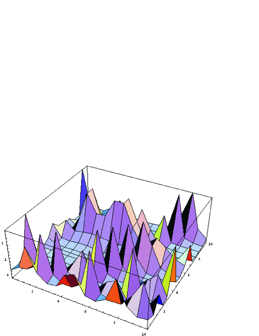
A three-dimensional plot of is displayed in Fig. 1, where an expected oscillatory behaviour can be seen. Not only the procedure based on the Milne phase function could compete very well with other approximate methods for the density of prime numbers but there is a further advantage on which we briefly comment in the following. As is well known, the Milne phase function enters as a basic ingredient in the Ermakov-Lewis phase-amplitude approach for parametric oscillator problems (for recent applications see [4]). To transform the Coulomb problem at hand
| (9) |
into a parametric dynamical problem for a unit mass classical particle, one can use the well-known map to canonical classical variables and leading to
| (10) |
| (11) |
where the coordinate plays the role of the classical Hamiltonian time. Various quantities, such as the Ermakov-Lewis invariant and geometrical angles can be calculated easily for this particularly interesting Coulomb problem (due to its connection with prime numbers). But we want to emphasize a different point here. In the parametric oscillator interpretation and of as Hamiltonian time, one can use as a direct tool for time-energy (and therefore time-imaginary axis) characterization of the density of prime numbers as can be inferred from Fig. 1.
References
References
- [1] Bhaduri M T C Khare A and Law D B 1995 Phys. Rev. E52 486, chao-dyn/9406006
- [2] Korsch H J 1985 Phys. Lett. A109 313
- [3] Espinoza P B 2000 Ermakov-Lewis dynamic invariants with some applications, Master thesis supervised by Rosu H C, math-ph/0002005
- [4] Rosu H C 2002 Physica Scripta 65 296, quant-ph/0104003; Rosu H C and Espinoza P 2001 Phys. Rev. E63 037603, physics/0004014; Hawkins R M and Lidsey J E 2002 Phys. Rev. D66 023523