Random matrix theory and the zeros of $\zeta\,^{\prime}(s)$

Abstract

We study the density of the roots of the derivative of the characteristic polynomial $Z(U,z)$ of an $N\times N$ random unitary matrix with distribution given by Haar measure on the unitary group. Based on previous random matrix theory models of the Riemann zeta function $\zeta(s)$, this is expected to be an accurate description for the horizontal distribution of the zeros of $\zeta\,^{\prime}(s)$ to the right of the critical line. We show that as $N\rightarrow\infty$ the fraction of the roots of $Z\,^{\prime}(U,z)$ that lie in the region $1-x/(N-1)\leq\left|z\right|<1$ tends to a limit function. We derive asymptotic expressions for this function in the limits $x\rightarrow\infty$ and $x\rightarrow 0$ and compare them with numerical experiments.

• 5 November 2002

• Mathematics Subject Classification: 15A52, 11M99

1 Introduction

We study the density of the roots of

$$Z\,^{\prime}(U,z)=\frac{\rmd}{\rmd z}\det(Iz-U)=\frac{\rmd}{\rmd z}\prod_{j=1}^{N}\left(z-\rme^{\rmi\theta_{j}}\right),\quad z\in\mathbb{C},$$

where $U$ is a random $N\times N$ unitary matrix, with respect to the circular unitary ensemble (CUE) of random matrix theory (RMT). Our main motivation is to investigate the horizontal distribution of the zeros of the derivative of the Riemann zeta function.

The zeta function is defined by

$$\zeta(s)=\sum_{n=1}^{\infty}\frac{1}{n^{s}},\quad\sigma=\mathop{\mathrm{Re}}\nolimits(s)>1,$$

and has an analytic continuation in the rest of the complex plane except for a simple pole at $s=1$. There are infinitely many non-trivial solutions to the equation $\zeta(s)=0$ in the strip $0<\sigma<1$; the Riemann hypothesis (RH) states that they all lie on the critical line $\sigma=1/2$. The interest in the horizontal distribution of the zeros of $\zeta\,^{\prime}(s)$ is motivated by its connection with RH. In 1934 Speiser [1] showed that RH is equivalent to $\zeta\,^{\prime}(s)$ having no zeros in the region $0<\sigma<1/2$. Furthermore, up to now the most efficient ways of computing the fraction the of zeros of the Riemann zeta function on the the critical line are based on what is known as Levinson’s method [2]; it turns out that the zeros of $\zeta\,^{\prime}(s)$ close to the critical line have a significant effect on the efficiency of this technique [4], therefore it is important to know how they are distributed. Levinson and Montgomery [5] proved a quantitative refinement of Speiser’s theorem, namely that $\zeta(s)$ and $\zeta\,^{\prime}(s)$ have essentially the same number of zeros to the left of $\sigma=1/2$, and showed that as $T\rightarrow\infty$, where $T$ is the height on the critical line, a positive proportion of the zeros of $\zeta\,^{\prime}(s)$ are in the region

$$\sigma<\frac{1}{2}+(1+\epsilon)\frac{\log\log T}{\log T},\quad\epsilon>0.$$

Subsequent improvements of Levinson and Montgomery’s results, first by Conrey and Ghosh [4], then by Guo [6], Soundararajan [7] and recently by Zhang [8] have established that a typical zero of $\zeta\,^{\prime}(s)$ tends to be much closer to the critical line and that conditionally on RH a positive proportion lie in the region

$$\sigma<\frac{1}{2}+\frac{C}{\log T},$$

for some positive constant $C$. Their distribution, however, is still unknown. Other results on the zeros of $\zeta\,^{\prime}(s)$ can be found in [9].

Over the past thirty years, overwhelming evidence has been accumulated which suggests that the local correlations of the non-trivial zeros of $\zeta(s)$ coincide, as $T\rightarrow\infty$, with those of the eigenvalues of hermitian matrices of large dimensions from the Gaussian unitary ensemble (GUE) [14]. As $N\rightarrow\infty$, the GUE statistics are in turn the same as those of the phases of the eigenvalues of $N\times N$ unitary matrices, on the scale of their mean distance $2\pi/N$, averaged over the CUE ensemble. More recently, however, it was realized that RMT not only describes with high accuracy the distribution of the Riemann zeros, but that it also provides techniques to make predictions and computations about the Riemann zeta function and certain classes of L-functions that previous methods had not been able to tackle. This started with the work of Keating and Snaith [30] on moments of the Riemann zeta function and other L-functions. Their key observation was that the locally determined statistical properties of $\zeta(s)$ high up the critical line can be modelled by characteristic polynomials $Z(U,z)$ of random unitary matrices $U$. In this model the two asymptotic parameters, $T$ for $\zeta(s)$ and $N$ for $U$, are compared by setting the densities of the zeros of $\zeta(s)$ and of the eigenvalues of $U$ equal, i.e.

$$N=\log\frac{T}{2\pi}.$$

This approach has since been extremely successful [32].

Following the same ideas, in this paper we suggest that the density $\rho(z)$ of the roots of $Z\,^{\prime}(U,z)$ will accurately describe the distribution of the zeros of $\zeta\,^{\prime}(s)$. A classical theorem in complex analysis states that if $p(z)$ is a polynomial, then the roots of $p\,^{\prime}(z)$ that are not roots of $p(z)$ lie all in the interior or on the boundary of the smallest convex polygon containing the zeros of $p(z)$ (see, e.g., [41]). Therefore, since the eigenvalues of a unitary matrix have modulus one, the solutions of the equation $Z\,^{\prime}(U,z)=0$ that are not zeros of $Z(U,z)$ are all inside the unit circle. If $s=1/2+\rmi t+u$, $t\in\mathbb{R}$, denotes the point at which $\zeta\,^{\prime}(s)$ is evaluated, then the region of $\mathbb{C}$ to the right of the critical line is mapped inside the unit circle by the conformal mapping $z=\rme^{-u}$. Thus, the radial density

$$\int_{0}^{2\pi}\left|z\right|\rho(z)\;\rmd\phi$$

becomes the analogue of the horizontal distribution of the zeros of $\zeta\,^{\prime}(s)$ to the right of the line $\sigma=1/2$. However, instead of $\rho(z)$, it turns out to be more convenient to consider $\mathop{\mathrm{Ip}}\nolimits(x)$, the fraction of the roots in the annulus $1-x/(N-1)\leq\left|z\right|<1$, where $x$ is the scaled distance from the unit circle. Our main results concern the asymptotics of $\mathop{\mathrm{Ip}}\nolimits(x)$. We show that as $N$ increases the roots of $Z\,^{\prime}(U,z)$ approach the unit circle, and $\mathop{\mathrm{Ip}}\nolimits(x)$ tends to a function independent of $N$. Furthermore, we obtain the following asymptotics as $N\rightarrow\infty$:

$$\mathop{\mathrm{Ip}}\nolimits(x)\sim 1-1/x,\quad x\rightarrow\infty,\quad x={\rm o}(N),$$

$$\mathop{\mathrm{Ip}}\nolimits(x)=\frac{8}{9\pi}\;x^{3/2}-\frac{64}{225\pi}\;x^{5/2}+\frac{128}{2205\pi}\;x^{7/2}+\Or(x^{4}).$$

These formulae are then tested numerically.

The paper is organized as follows: in section 2 we introduce the mathematical problem and describe the main properties of the roots of $Z\,^{\prime}(U,z)$; in section 3 the asymptotics of $\mathop{\mathrm{Ip}}\nolimits(x)$ as $x\rightarrow\infty$ are computed; using heurstic arguments, in section 4, $\mathop{\mathrm{Ip}}\nolimits(x)$ is derived in the limit $x\rightarrow 0$; section 5 concludes the paper with final remarks.

2 The distribution of the roots of $Z\,^{\prime}(U,z)$

The CUE ensemble of RMT is defined as the space ${\rm U}(N)$ of $N\times N$ unitary matrices endowed with a probability measure $\rmd\mu(U)$ invariant under any inner automorphism

$$U\mapsto VUW,\quad U,V,W\in{\rm U}(N).$$

In other words, $\rmd\mu(U)$ must be invariant under left and right multiplication by elements of ${\rm U}(N)$, so that each matrix in the ensemble is equally weighted. There exists a unique measure on the unitary group ${\rm U}(N)$ with this property, known as Haar measure. The infinitesimal volume element of the CUE ensemble occupied by those matrices whose eigenvalues have phases lying between $\boldsymbol{\theta}=(\theta_{1},\theta_{2},\ldots,\theta_{N})$ and $\boldsymbol{\theta}+\rmd^{N}\boldsymbol{\theta}$ is given by

$$\Omega(N)\Delta^{2}(\boldsymbol{\theta})\rmd^{N}\boldsymbol{\theta},$$ (2.1)

where

$$\Delta(\boldsymbol{\theta})=\prod_{1\,\leq j\,<\,k\,\leq\,N}\left|\rme^{\rmi\theta_{j}}-\rme^{\rmi\theta_{k}}\right|\quad{\rm and}\quad\Omega(N)=\frac{1}{(2\pi)^{N}N!}.$$

Our goal in this paper is to study the density of the roots of $Z\,^{\prime}(U,z)$, where $U$ is a random unitary matrix with distribution given by (2.1). The analogous problem for the Ginibre ensemble has been studied by Dennis and Hannay [42].

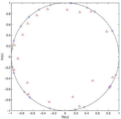
(a) $N=20$

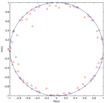
(b) $N=50$

Figure 1: Zeros of characteristic polynomials of random unitary matrices (□) and of their derivatives (△).

In figure 1 are plotted the zeros of the characteristic polynomials $Z(U,z)$ and of their derivatives of two unitary matrices taken at random with respect to Haar measure for $N=20$ and $N=50$. Such matrices can be easily generated numerically by taking complex matrices whose entries are independent complex random numbers with Gaussian distribution, and then by applying Gram-Schmidt orthogonalization to the rows or columns (see, e.g., [43]). There are a few qualitative features that can be immediately observed. Firstly, since the distribution (2.1) is translation invariant on the unit circle, the density of the roots of $Z\,^{\prime}(U,z)$ depends only on the distance from the origin. Secondly, as mentioned in the introduction, the roots of $Z\,^{\prime}(U,z)$ are all inside the unit circle. This property can be easily understood with the following argument. Let $z_{1},z_{2},\ldots,z_{N}$ be $N$ complex numbers; if they all are on the same side of a straight line passing through the origin, then

$$z_{1}+z_{2}+\cdots+z_{N}\neq 0\quad{\rm and}\quad\frac{1}{z_{1}}+\frac{1}{z_{2}}+\cdots+\frac{1}{z_{N}}\neq 0.$$ (2.2)

Let $\{z_{j}\}_{j=1}^{N}$ be the roots of a polynomial $p(z)$ and $z$ a point outside the smallest convex polygon containing $\{z_{j}\}_{j=1}^{N}$. Now, consider a straight line passing through $z$ and lying outside such a polygon. Because of equation (2.2), the logarithmic derivative

$$\frac{p\,^{\prime}(z)}{p(z)}=\frac{1}{z-z_{1}}+\frac{1}{z-z_{2}}+\cdots+\frac{1}{z-z_{N}}$$

cannot vanish. There are two others less obvious features that figure 1 reveals and that become more apparent as $N$ increases: firstly, the roots of $Z\,^{\prime}(U,z)$ concentrate in a small region in proximity of the the unit circle; secondly, given two consecutive zeros of $Z(U,z)$, say $\rme^{\rmi\theta_{j}}$ and $\rme^{\rmi\theta_{j+1}}$, close to each other, there often appears to be a root of $Z\,^{\prime}(U,z)$ near the midpoint

$$\frac{\rme^{\rmi\theta_{j}}+\rme^{\rmi\theta_{j+1}}}{2}.$$ (2.3)

In the following sections we shall give quantitative interpretations of these properties.

Let us set $u=\mathop{\mathrm{Re}}\nolimits{z}$ and $v=\mathop{\mathrm{Im}}\nolimits{z}$; furthermore, denote by $\{\lambda_{j}(\boldsymbol{\theta})\}_{j=1}^{N-1}$ the set of roots of $Z\,^{\prime}(U,z)$ and consider the linear functional

$$F[\tau]_{\lambda_{j}(\boldsymbol{\theta})}=\int_{\mathbb{C}}\tau(z)\boldsymbol{\delta}\left(z-\lambda_{j}(\boldsymbol{\theta})\right)\rmd^{2}z=\tau\left(\lambda_{j}(\boldsymbol{\theta})\right),$$

where $\rmd^{2}z=\rmd u\,\rmd v$ and $\tau(z)$ is an infinitely differentiable complex function whose partial derivatives with respect to $u$ and $v$ decrease faster than any power of $1/\left|z\right|$. Moreover,

$$\boldsymbol{\delta}\left(z-\lambda_{j}(\boldsymbol{\theta})\right)=\delta\left(u-\mathop{\mathrm{Re}}\nolimits\left(\lambda_{j}(\boldsymbol{\theta})\right)\right)\delta\left(v-\mathop{\mathrm{Im}}\nolimits\left(\lambda_{j}(\boldsymbol{\theta})\right)\right)$$

is the product of two Dirac delta functions with real arguments. Then, we have

$$\int_{\mathbb{C}}\tau(z)\rho(z)\,\rmd^{2}z=\frac{\Omega(N)}{N-1}\sum_{j=1}^{N-1}\int_{[0,\,2\pi]^{N}}\int_{\mathbb{C}}\tau(z)\,\boldsymbol{\delta}\left(z-\lambda_{j}(\boldsymbol{\theta})\right)\Delta^{2}(\boldsymbol{\theta})\rmd^{2}z\,\rmd^{N}\boldsymbol{\theta},$$

where the distribution

$$\rho(z):=\frac{\Omega(N)}{N-1}\sum_{j=1}^{N-1}\int_{[0,\,2\pi]^{N}}\boldsymbol{\delta}\left(z-\lambda_{j}(\boldsymbol{\theta})\right)\Delta^{2}(\boldsymbol{\theta})\rmd^{N}\boldsymbol{\theta}$$ (2.4)

defines the density of $\{\lambda_{j}(\boldsymbol{\theta})\}_{j=1}^{N-1}$ .

The main tool that we shall use to evaluate (2.4) is a basic identity that expresses Toeplitz determinants in terms of integrals over the unitary group. If

$$f(\theta)=\sum_{k=-\infty}^{\infty}\hat{f}_{k}\,\rme^{\rmi k\,\theta}$$

is a complex function on the unit circle, then we denote by $D_{N-1}[f]$ the determinant of the Toeplitz matrix

$$T_{N-1}[f]:=\left(\begin{array}[]{cccc}\hat{f}_{0}&\hat{f}_{1}&\cdots&\hat{f}_{N-1}\\ \hat{f}_{-1}&\hat{f}_{0}&\cdots&\hat{f}_{N-2}\\ \vdots&\vdots&&\vdots\\ \hat{f}_{-(N-1)}&\hat{f}_{-(N-2)}&\cdots&\hat{f}_{0}\end{array}\right).$$

Now, let $\Phi_{f}$ be a class function, i.e. a complex function on ${\rm U}(N)$ such that

$$\Phi_{f}\left(VUV^{-1}\right)=\Phi_{f}(U),\quad V,U\in{\rm U}(N).$$

Furthermore, suppose that

$$\Phi_{f}(U)=f(\theta_{1})f(\theta_{2})\cdots f(\theta_{N}),$$ (2.5)

where $\{\rme^{\rmi\theta_{j}}\}_{j=1}^{N}$ are the eigenvalues of $U$. The Heine-Szegő identity [44] states that

$$D_{N-1}[f] =\int_{{\rm U}(N)}\Phi_{f}(U)\,\rmd\mu(U)$$ (2.6)

$$=\Omega(N)\int_{[0,\,2\pi]^{N}}\left(\prod_{j=1}^{N}f(\theta_{j})\right)\Delta^{2}(\boldsymbol{\theta})\rmd^{N}\boldsymbol{\theta}.$$

In order to apply this formula, we must express the sum of delta functions in (2.4) as a product of the form (2.5). The zeros of $Z\,^{\prime}(U,z)$ that are not multiple roots of $Z(U,z)$ are the same as those of the logarithmic derivative of $Z(U,z)$. Since the set of unitary matrices with degenerate eigenvalues has zero measure, we rewrite the integrand in equation (2.4) as

$$\sum_{j=1}^{N-1}\boldsymbol{\delta}\left(z-\lambda_{j}\right)=\boldsymbol{\delta}\left(Z\,^{\prime}(U,z)/Z(U,z)\right)\left|\frac{\rmd}{\rmd z}\left[Z\,^{\prime}(U,z)/Z(U,z)\right]\right|^{2}.$$ (2.7)

In the next step we use the integral representation of a delta function:

$$\delta(x)=\frac{1}{2\pi}\int_{-\infty}^{\infty}\rme^{\rmi\xi x}\,\rmd\xi.$$

The complex delta function in the right-hand side of equation (2.7) now becomes

$$\boldsymbol{\delta}\left(Z\,^{\prime}(U,z)/Z(U,z)\right)=\frac{1}{4\pi^{2}}\int_{\mathbb{C}}\exp\left[\frac{\rmi}{2}\left(\frac{Z\,^{\prime}(U,z)}{Z(U,z)}\;\overline{w}+\frac{\overline{Z\,^{\prime}(U,z)}}{\overline{Z(U,z)}}\,w\right)\right]\rmd^{2}w.$$ (2.8)

Clearly, the identity (2.6) can be applied to the argument of the integral (2.8); furthermore, the Jacobian in equation (2.7) can be transformed into a product of the form (2.5) by using the following representation of the modulus square of a complex number:

$$\left|z\right|^{2}=-\left.\frac{\partial^{2}}{\partial\alpha^{2}}\;G(\alpha,z)\right|_{\alpha=0},\quad\alpha\in\mathbb{R},$$

where

$$G(z,\alpha):=\exp\left[\rmi\alpha\left(z+\overline{z}\,\right)/2\right]+\exp\left[\alpha\left(z-\overline{z}\,\right)/2\right].$$

Finally, the density (2.4) becomes

$$\rho(z)=-\frac{1}{4\pi^{2}\left(N-1\right)}$$

$$\qquad\quad\times\frac{\partial^{2}}{\partial\alpha^{2}}\left[\int_{\mathbb{C}}\Bigl{(}D_{N-1}[\exp(\rmi g)](w,\alpha,z)+D_{N-1}[\exp(\rmi h)](w,\alpha,z)\Bigr{)}\rmd^{2}w\right]_{\alpha=0},$$ (2.9)

where

$$g(\theta;w,\alpha,z):=\frac{1}{2}\left(\frac{\overline{w}}{z-\rme^{\rmi\theta}}+\frac{w}{\overline{z}-\rme^{-\rmi\theta}}\right)-\frac{\alpha}{2}\left(\frac{1}{\left(z-\rme^{\rmi\theta}\right)^{2}}+\frac{1}{\left(\overline{z}-\rme^{-\rmi\theta}\right)^{2}}\right)$$

and

$$h(\theta;w,\alpha,z):=\frac{1}{2}\left(\frac{\overline{w}}{z-\rme^{\rmi\theta}}+\frac{w}{\overline{z}-\rme^{-\rmi\theta}}\right)+\frac{\rmi\alpha}{2}\left(\frac{1}{\left(z-\rme^{\rmi\theta}\right)^{2}}-\frac{1}{\left(\overline{z}-\rme^{-\rmi\theta}\right)^{2}}\right)$$

are real functions.

3 Asymptotics of $\rho(z)$

Computing (2) exactly appears to be a formidable task. However, there exists a powerful theorem of Szegő that will allow us to compute the leading-order asymptotics of $\rho(z)$ as $N\rightarrow\infty$.

The strong Szegő limit theorem. Let

$$\eta(\theta)=\sum_{k=-\infty}^{\infty}\hat{\eta}_{k}\,\rme^{\rmi k\,\theta}$$

be a complex function on the unit circle. If the series

$$\sum_{k=-\infty}^{\infty}\left|\hat{\eta}_{k}\right|\quad{\it and}\quad\sum_{k=-\infty}^{\infty}\left|k\right|\left|\hat{\eta}_{k}\right|^{\,2}$$ (3.1)

converge, then

$$D_{N-1}[\exp(\eta)]=\exp\left(\hat{\eta}_{0}N+\sum_{k=1}^{\infty}k\,\hat{\eta}_{-k}\hat{\eta}_{k}+{\rm o}(1)\right),\quad N\rightarrow\infty.$$ (3.2)

The first proof of this theorem was given by Szegő in [45] under stronger conditions; several proofs have since been developed [46, 51].

In the region $\left|z\right|<1$, $g(\theta;w,\alpha,z)$ and $h(\theta;w,\alpha,z)$ are just sums of geometric series and of their derivatives whose Fourier coefficients can be easily computed. We have

$$g(\theta;w,\alpha,z)=\sum_{k=-\infty}^{\infty}\hat{g}_{k}\,\rme^{\rmi k\theta}\quad{\rm and}\quad h(\theta;w,\alpha,z)=\sum_{k=-\infty}^{\infty}\hat{h}_{k}\,\rme^{\rmi k\theta},$$

where

$$\hat{g}_{0}=0,\quad\hat{g}_{k}=-\frac{w}{2}\overline{z}^{\;k-1}-\frac{\alpha}{2}\left(k-1\right)\overline{z}^{\;k-2},\quad k\in\mathbb{Z}^{+}$$

and

$$\hat{h}_{0}=0,\quad\hat{h}_{k}=-\frac{w}{2}\overline{z}^{\;k-1}-\frac{\rmi\alpha}{2}\left(k-1\right)\overline{z}^{\;k-2},\quad k\in\mathbb{Z}^{+}.$$

Since $g(\theta;w,\alpha,z)$ and $h(\theta;w,\alpha,z)$ are real, $\hat{g}_{-k}=\overline{\hat{g}}_{k}$ and $\hat{h}_{-k}=\overline{\hat{h}}_{k}$. Computing the argument in the exponential of equation (3.2) involves only summing and differentiating geometric series. We obtain

$$E(g)=\sum_{k=1}^{\infty}k\,\left|\hat{g}_{k}\right|^{2} =c(w,\alpha,r)+\frac{\alpha\mathop{\mathrm{Re}}\nolimits(w\overline{z})}{\left(1-r^{2}\right)^{3}},$$ (3.3a)

$$E(h)=\sum_{k=1}^{\infty}k\,\left|\hat{h}_{k}\right|^{2} =c(w,\alpha,r)+\frac{\alpha\mathop{\mathrm{Im}}\nolimits(w\overline{z})}{\left(1-r^{2}\right)^{3}},$$ (3.3b)

where $r=\left|z\right|$ and

$$c(w,\alpha,r)=\frac{\left|w\right|^{\,2}}{4}\frac{1}{\left(1-r^{2}\right)^{2}}+\frac{\alpha^{2}}{2}\left[\frac{3r^{2}}{\left(1-r^{2}\right)^{4}}+\frac{1}{\left(1-r^{2}\right)^{3}}\right].$$

As a consequence, the second sum in (3.1) is finite. Furthermore, we have

$$\lim_{k\rightarrow\infty}\left|\frac{\hat{g}_{k+1}}{\hat{g}_{k}}\right|=\lim_{k\rightarrow\infty}\left|\frac{\hat{h}_{k+1}}{\hat{h}_{k}}\right|=r<1.$$

Hence, the first series in (3.1) converges too, and the strong Szegő limit theorem applies.

When computing derivatives of the asymptotics of the integral (2), care must be taken that the error term does not become comparable or even greater than the leading-order term. This could happen, for example, if the remainder were a highly oscillatory function of $\alpha$. It turns out that the convergence of $D_{N-1}[\exp(\rmi g)]$ and $D_{N-1}[\exp(\rmi h)]$ to (3.2) is so fast that the derivatives of the error term remain small. This is proved in the appendix.

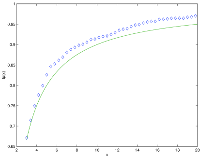
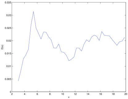
Figure 2: Comparison (a) and difference (b) between $\mathop{\mathrm{Ip}}\nolimits(x)$ computed numerically for $N=800$ (◇) and formula (3) (——).

In equation (2) the second derivative commutes with the integral, hence differentiating twice with respect to $\alpha$ gives

$$\frac{\partial^{2}}{\partial\alpha^{2}}\Biggl{[}D_{N-1}[\exp(\rmi g)](w,\alpha,z)+D_{N-1}[\exp(\rmi h)](w,\alpha,z)\Biggr{]}_{\alpha=0}$$

$$\sim\left[\frac{\left|w\right|^{2}r^{2}}{\left(1-r^{2}\right)^{6}}-\frac{6r^{2}}{\left(1-r^{2}\right)^{4}}-\frac{2}{\left(1-r^{2}\right)^{3}}\right]\exp\left[-\frac{\left|w\right|^{2}}{4\left(1-r^{2}\right)^{2}}\right],\quad N\rightarrow\infty.$$

This expression can be trivially integrated. Finally, we obtain

$$\rho(z)\sim\frac{2}{\pi\left(N-1\right)\left(1-r^{2}\right)^{2}}\,,\quad N\rightarrow\infty.$$

As anticipated, $\rho(z)$ depends only on the distance from the origin $r$ and is asymptotically concentrated in a small region near the unit circle, which explains the migration of the roots of $Z\,^{\prime}(U,\lambda)$ observed in figure 1 as $N$ increases. Since $\rho(z)$ is a density, it must be normalized to one, therefore we require

$$\int_{0}^{2\pi}\int_{0}^{1-\epsilon}r\rho(z)\,\rmd r\rmd\phi\sim 1,\quad N\rightarrow\infty,\quad\epsilon\rightarrow 0.$$

Let us now define $\mathop{\mathrm{Ip}}\nolimits(x)$ to be the fraction of the zeros in the annulus
$1-x/(N-1)\leq r<1$, where $x={\rm o}(N)$, i.e.

$$\mathop{\mathrm{Ip}}\nolimits(x)=1-\int_{0}^{2\pi}\int_{0}^{1-x/(N-1)}r\rho(z)\,\rmd r\rmd\phi\sim 1-\frac{2}{N-1}\left[\frac{1}{1-r^{2}}\right]_{0}^{1-x/(N-1)}$$

$$\hbox to0.0pt{\hss${}\sim{}$}1-1/x,\quad N\rightarrow\infty,\quad x\rightarrow\infty.$$ (3.3d)

As $N\rightarrow\infty$ the leading-order term of $\mathop{\mathrm{Ip}}\nolimits(x)$ is independent of $N$. Equation (3) is the main result of this section. In figure 2 formula (3) is compared with $\mathop{\mathrm{Ip}}\nolimits(x)$ computed for a matrix of dimension $N=800$.

4 The asymptotics $x\rightarrow 0$

The small $x$ asymptotics of $\mathop{\mathrm{Ip}}\nolimits(x)$ requires first the evaluation of the limit $x\rightarrow 0$ and then of the limit $N\rightarrow\infty$. Szegő’s theorem gives an asymptotic expression as $N\rightarrow\infty$ before the limit $x\rightarrow 0$ can be taken, therefore provides information only for relatively large $x$. In order to determine $\mathop{\mathrm{Ip}}\nolimits(x)$ in the limit $x\rightarrow 0$, the integral in equation (2) needs to be evaluated for finite $N$. Such computation seems to be an extremely difficult task: the integrand has essential singularities that usual techniques in RMT and complex analysis cannot tackle. Notwithstanding such obstacles, it turns out that $\mathop{\mathrm{Ip}}\nolimits(x)$ can be derived in the limit $x\rightarrow 0$ with the help of a heuristic argument.

As was mentioned in section 2, from figure 1 it appears that if $\rme^{\rmi\theta_{j}}$ and $\rme^{\rmi\theta_{j+1}}$ are two consecutive roots of $Z(U,z)$ which are close to each other, then as $N\rightarrow\infty$ there is often a root of $Z\,^{\prime}(U,z)$ near the midpoint (2.3). Thus, one might be led to assume that for small $x$ the distance from the origin $r$ is distributed like

$$1-x/(N-1) =\left|\frac{\rme^{\rmi\theta_{j}}+\rme^{\rmi\theta_{j+1}}}{2}\right|=\frac{\sqrt{2+2\cos\left(2\pi S/N\right)}}{2}$$ (3.3a)

$$\approx 1-\frac{\pi^{2}S^{\,2}}{2N^{2}},\quad 1\leq j\leq N,$$

where $S$ is the rescaled distance, or spacing, between phases of consecutive eigenvalues, i.e.

$$S=\frac{N}{2\pi}\left|\theta_{j+1}-\theta_{j}\right|,\quad 1\leq j\leq N.$$

This is trivially true only for $N=2$; since $S=\Or(1)$, for $N>2$ equation (3.3a) would imply an average distance of the zeros of $Z\,^{\prime}(U,z)$ from the unit circle of order $1/N^{2}$, and therefore a dependence of $\mathop{\mathrm{Ip}}\nolimits(x)$ on $N$ even at the leading order, which contradicts the numerics reported in figure 5 and formula (3).

It turns out that behaviour of $\mathop{\mathrm{Ip}}\nolimits(x)$ as $x\rightarrow 0$ can be understood using Dyson’s electrostatic model for the CUE ensemble (see, e.g., [52]). The zeros of $Z(U,z)$ can be interpreted as $N$ unit charges confined in a two-dimensional universe and moving in a thin circular conducting wire of radius one. The electric field generated at any point in the complex plane by this Coulomb gas is just the complex conjugate of the logarithmic derivative of $Z(U,z)$, i.e.

$$\mathbf{E}(z)=\frac{1}{\overline{z}-\rme^{-\rmi\theta_{1}}}+\frac{1}{\overline{z}-\rme^{-\rmi\theta_{2}}}+\cdots+\frac{1}{\overline{z}-\rme^{-\rmi\theta_{N}}}.$$

Hence, the zeros of $Z\,^{\prime}(U,z)$ are located where $\mathbf{E}(z)$ vanishes. Now, the field at point $q$, whose distance from the unit circle is of order $1/N$, can be separated into two components: the first one is the field of the two charges closest to $q$, let us denote them by A and B, whose strength is clearly of order $N$; the second one is the field generated by the other $N-2$ charges. As $N$ increases, $q$ approaches the unit circle, and the latter component of $\mathbf{E}(q)$ can be approximated by the field of a continuous circular charge distribution with density $\mu=N/(2\pi)$, i.e.

$$\mathbf{E}(q)\approx\mathbf{E}_{\mu}(q)+\mathbf{E}_{{\rm AB}}(q),$$ (3.3b)

where $\mathbf{E}_{\mu}(q)$ is the field generated by $\mu$ and $\mathbf{E}_{{\rm AB}}(q)$ the one determined by A and B. For large $N$, $\mathbf{E}_{\mu}(q)$ and $\mathbf{E}_{{\rm AB}}(q)$ have approximately opposite directions, thus $\mathbf{E}(z)$ might vanish at $q$ only if $\left|\mathbf{E}_{\mu}(q)\right|=\Or(N)$. This situation is described schematically in figure 3.

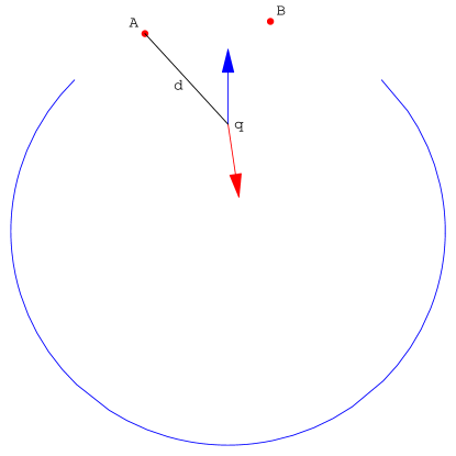
Figure 3: Schematic representation of the two components $\mathbf{E}_{\mu}(q)$ and $\mathbf{E}_{{\rm AB}}(q)$ of the electric field (3.3b) at a point $q$ close to the unit circle in Dyson’s electrostatic model.

Determining the order of magnitude of $\mathbf{E}_{\mu}(q)$ is a simple exercise in electrostatics. If the continuous charge distribution filled the whole unit circle, the field inside it would be zero. Thus, by linearity $\mathbf{E}_{\mu}(q)$ is equal and opposite to the field of a circular arc $[-\tilde{\theta},\tilde{\theta}]$ with charge density $\mu$ and containing no more than four eigenvalues. We have

$$\left|\mathbf{E}_{\mu}(q)\right|=\frac{N}{2\pi}\int_{-\tilde{\theta}}^{\tilde{\theta}}\,\frac{1}{d(\theta)}\sqrt{1-\frac{\sin^{2}\theta}{d(\theta)^{2}}}\,\rmd\theta,$$

where $d(\theta)$ is the distance between $q$ and $\rme^{\rmi\theta}$. By setting $d(\theta)=t(\theta)/N$, with $t(\theta)=\Or(1)$, and applying the mean value theorem we obtain

$$\left|\mathbf{E}_{\mu}(q)\right|=\frac{\tilde{\theta}N^{2}}{\pi t(\xi)}\sqrt{1-\frac{\sin^{2}\xi}{d(\xi)^{2}}},\quad-\tilde{\theta}\leq\xi\leq\tilde{\theta}.$$

Since the length of the interval $[-\tilde{\theta},\tilde{\theta}]$ is of the order of few level spacings, $\tilde{\theta}=\Or(1/N)$ and $\left|\mathbf{E}_{\mu}(q)\right|=\Or(N)$.

The field $\mathbf{E}_{{\rm AB}}(z)$ vanishes at the midpoint (2.3), but for large $N$ the presence of $\mathbf{E}_{\mu}(z)$ shifts the zeros of $\mathbf{E}(z)$ at a distance of order $1/N$ from the unit circle. Since at first approximation the contribution of $\mathbf{E}_{\mu}(z)$ does not depend on the spacing $S$, from (3.3a) it is reasonable to assume that as $x\rightarrow 0$ the distance of the zeros of $Z\,^{\prime}(U,z)$ from the unit circle is approximately distributed like $S^{\,2}/N$. Hence, we shall conjecture that

$$x\sim\beta\,\frac{\pi^{2}S^{\,2}}{2}\,,\quad x\rightarrow 0,$$ (3.3c)

where $\beta$ is a constant independent of $N$.

From equation (3.3c) it is straightforward to derive an asymptotics expression for $\mathop{\mathrm{Ip}}\nolimits(x)$ as $x\rightarrow 0$. We have

$$\mathop{\mathrm{Ip}}\nolimits(x)\sim\int_{0}^{x}\gamma(y)\,\rmd y,\quad x\rightarrow 0,$$

where

$$\gamma(y):=\frac{1}{\pi}\sqrt{\frac{1}{2\beta y}}\,P_{{\rm CUE}}\left[\frac{1}{\pi}\left(\frac{2y}{\beta}\right)^{1/2}\right]$$

and $P_{{\rm CUE}}(S)$ is the CUE spacing distribution in the limit $N\rightarrow\infty$, i.e.

$$P_{{\rm CUE}}(S):=\lim_{N\rightarrow\infty}P_{{\rm CUE}}(N;S).$$

$P_{{\rm CUE}}(S)$ has a power series expansion with infinite radius of convergence:

$$P_{{\rm CUE}}(S)=\sum_{l=0}^{\infty}(l+4)(l+3)E_{l}\,S^{2+l}.$$ (3.3d)

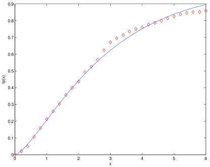
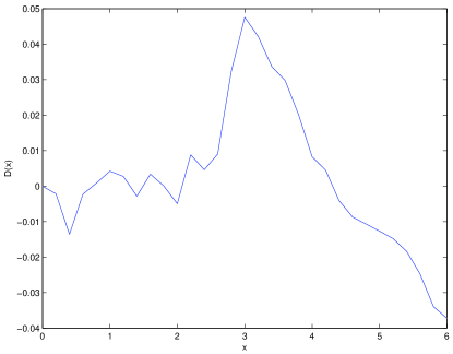
Figure 4: Comparison (a) and difference (b) between $\mathop{\mathrm{Ip}}\nolimits(x)$ computed numerically for $N=800$ (◇) and the one defined by the series (3.3e) truncated at $l=30$ and with $\beta=1/2$ (——).

There exist efficient algorithms for computing the coefficients $E_{l}$ (see, e.g., [53]), which with symbolic mathematical packages can be evaluated exactly up to very high values of $l$. Using (3.3d) one can easily obtain a series expansion for $\mathop{\mathrm{Ip}}\nolimits(x)$:

$$\mathop{\mathrm{Ip}}\nolimits(x)\sim\sum_{l=0}^{\infty}\left(\frac{2}{\beta\pi^{2}}\right)^{\frac{l+3}{2}}(l+4)\;E_{l}\;x^{\frac{l+3}{2}},\quad x\rightarrow 0.$$ (3.3e)

Now we have to determine the parameter $\beta$, which can be found only empirically. It turns out that if we set $\beta=1/2$ there exists an astonishing agreement between (3.3e) and numerics in the region where the large $x$ asymptotics is not valid. This is shown in figure 4.

Notwithstanding the accuracy with which the series (3.3e) models the numerical data, it can be expected to approximate $\mathop{\mathrm{Ip}}\nolimits(x)$ only for small $x$; indeed, it tends to one much faster than $1-1/x$. Furthermore, in deriving (3.3e) we have implicitly assumed that the main contribution to $\mathop{\mathrm{Ip}}\nolimits(x)$ comes only from the two zeros of $Z(U,z)$ closest to a given root of $Z\,^{\prime}(U,z)$; we now need to estimate in what region this assumption is justified.

Let us consider $k+2$ successive eigenvalues of a unitary matrix. Since Haar measure is translation invariant on the unit circle, the corrections to (3.3e) will depend by all possible rescaled distances

$$S_{k}=\frac{N}{2\pi}\left|\theta_{j+k+1}-\theta_{j}\right|,\quad 1\leq j\leq N.$$

However, as $S_{k}\rightarrow 0$, the limit densities $P_{{\rm CUE}}(S_{k})$ go to zero very fast, hence the dependence on $S_{k}$ does not affect the first few terms of the series (3.3e). For example, consider three consecutive zeros of $Z(U,z)$ close to each other, say

$$\exp\left(\frac{2\pi\rmi}{N}\,\alpha\right),\quad\exp\left(\frac{2\pi\rmi}{N}\,\left(\alpha+S_{0}\right)\right)\quad{\rm and}\quad\exp\left(\frac{2\pi\rmi}{N}\,\left(\alpha+S_{1}\right)\right),\quad S_{1}\geq S_{0}\geq 0.$$

Simple algebra and Dyson’s model indicate that the rescaled distance $x$ should be distributed like

$$\beta^{\prime}(S_{0}+S_{1})^{2},$$

for some constant $\beta^{\prime}$ independent of $N$. It turns out that

$$P_{{\rm CUE}}(S_{1})=\frac{\pi^{6}S_{1}^{\,7}}{4050}+\Or(S_{1}^{\,8}),$$ (3.3f)

which suggests that the contributions to (3.3e) due to $S_{1}$ leave the coefficients of the terms $x^{d}$ with $d<4$ unchanged. For $k>1$, $P_{{\rm CUE}}(S_{k})$ goes to zero as $S_{k}\rightarrow 0$ even faster than (3.3f). These considerations and formula (3.3e) give the following expression for the asymptotic expansion of $\mathop{\mathrm{Ip}}\nolimits(x)$:

$$\mathop{\mathrm{Ip}}\nolimits(x)=\frac{8}{9\pi}\;x^{3/2}-\frac{64}{225\pi}\;x^{5/2}+\frac{128}{2205\pi}\;x^{7/2}+\Or(x^{4}).$$

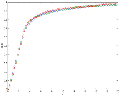
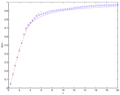
Figure 5: (a) Fraction of zeros of $Z\,^{\prime}(U,z)$ in the region $1-x/(N-1)\leq\left|z\right|<1$ for $N=800$ (◇), $N=500$ (○) and $N=400$ (△). (b) Same data as in (a) for $N=800$ (◇) compared with formula (3) (——) and with the series (3.3e) truncated at $l=30$ and with $\beta=1/2$ (-  -  -  -).

However, from the agreement with numerics observed in figure 4 and 5, we would expect that the corrections to the series (3.3e) should be negligible up to terms of order much higher than $x^{4}$.

The integrated distribution $\mathop{\mathrm{Ip}}\nolimits(x)$ is plotted in figure 5 for zeros of $Z\,^{\prime}(U,z)$ computed numerically for random unitary matrices of various dimensions; clearly, $\mathop{\mathrm{Ip}}\nolimits(x)$ tends to a limit function. Figure 5 shows that equation (3) and the series (3.3e) together, although asymptotic formulae, approximate $\mathop{\mathrm{Ip}}\nolimits(x)$ with high accuracy for all $x\geq 0$.

5 Concluding remarks

We have investigated the density $\rho(z)$ of the roots of $Z\,^{\prime}(U,z)$, where $Z(U,z)$ is the characteristic polynomial of a random $N\times N$ unitary matrix with distribution given by Haar measure on the unitary group. Since the locally determined statistical properties of the Riemann zeta function high up the critical line can be modelled by $Z(U,z)$, it is expected that $\rho(z)$ will accurately describe the behaviour of the zeros of $\zeta\,^{\prime}(s)$. It turns out that instead of $\rho(z)$, it is more convenient to study $\mathop{\mathrm{Ip}}\nolimits(x)$, the fraction of the roots in the region $1-x/(N-1)\leq\left|z\right|<1$. In the analogous problem for the zeta function, this is equivalent to looking at the fraction of the zeros of $\zeta\,^{\prime}(s)$ in the region $1/2<\sigma\leq 1/2+x/\log T$ where $\sigma=\mathop{\mathrm{Re}}\nolimits(s)$ and $T$ is the height on the critical line. It is shown that as $N\rightarrow\infty$, $\mathop{\mathrm{Ip}}\nolimits(x)$ becomes independent of $N$.

The density $\rho(z)$ can be defined as the average over ${\rm U}(N)$ of the sum of delta functions

$$\frac{1}{N-1}\sum_{j=1}^{N-1}\boldsymbol{\delta}\left(z-\lambda_{j}(\boldsymbol{\theta})\right),$$

where the $\lambda_{j}(\boldsymbol{\theta})$ are the zeros of $Z\,^{\prime}(U,z)$. The behaviour of $\mathop{\mathrm{Ip}}\nolimits(x)$ for large $x$ can be computed by applying standard techniques for integrals over ${\rm U}(N)$. The sum of Dirac deltas can be manipulated in such a way that eventually the average over ${\rm U}(N)$ is reduced to the computation of the second derivative of an integral over the complex plane of the sum of two Toeplitz determinants. Furthermore, the integrand satisfies the hypothesis of the strong Szegő limit theorem, which gives a simple asympotic expression for such determinants. Further simple manipulations lead to

$$\mathop{\mathrm{Ip}}\nolimits(x)\sim 1-1/x,\quad x={\rm o}(N),\quad x\rightarrow\infty.$$

The limits $x\rightarrow 0$ and $N\rightarrow\infty$ do not commute; the evaluation of the asymptotics of $\mathop{\mathrm{Ip}}\nolimits(x)$ as $x\rightarrow 0$ requires first the computation of the limit $x\rightarrow 0$ and then of the limit $N\rightarrow\infty$. The application of Szegő’s theorem clearly prevents this, therefore provides information only for relative large $x$. However, Dyson’s electrostatic model for the CUE ensemble leads naturally to the assumptions that for small $x$, as $N\rightarrow\infty$, the distance of the roots of $Z\,^{\prime}(U,z)$ from the unit circle is on average of order $1/N$ and is distributed like the square of the spacings between phases of consecutive eigenvalues of unitary matrices in the CUE ensemble (appropriately rescaled). These two simple hypotheses give a conjecture for $\mathop{\mathrm{Ip}}\nolimits(x)$ as $x\rightarrow 0$ whose agreement with numerical experiments covers with high accuracy the region where the large $x$ asymptotics fails.

Unfortunately, the zeros of $\zeta\,^{\prime}(s)$ are poorly understood, and there is not even a conjecture for their horizontal distribution to compare with the results derived in this paper. Given that it seems extremely difficult to obtain an analytical expression of such a quantity, we believe that it would be interesting and worthwhile to conduct a thorough numerical study as independent verification of the model presented here.

Appendix. Derivatives of Szegő’s strong asymptotic formula

In this appendix we show that in the cases considered in the present paper, the error term in formula (3.2) remains small when differentiated with respect to $\alpha$; in other words, we want to prove that

$$\frac{\partial^{2}}{\partial\alpha^{2}}\Biggl{[}D_{N-1}[\exp(\rmi g)](\alpha)+D_{N-1}[\exp(\rmi h)](\alpha)\Biggr{]}_{\alpha=0}$$

$$\sim\frac{\partial^{2}}{\partial\alpha^{2}}\Biggl{[}\,\exp\left(-E(g)\right)+\exp\left(-E(h)\right)\Biggr{]}_{\alpha=0},\quad N\rightarrow\infty,$$ (A1)

where $E(g)$ and $E(h)$ are defined in equations (3.3). The main idea of the proof is quite simple: we first represent the Toeplitz determinants with exact formulae and differentiate them with respect to $\alpha$; then we take the limit $N\rightarrow\infty$. We shall consider only $D_{N-1}[\exp(\rmi g)]$, as the proof for $D_{N-1}[\exp(\rmi h)]$ is completely analogous.

The identity (2.6) allows us to write

$$D_{N-1}[\exp(\rmi g)](\alpha)=\int_{{\rm U}(N)}\exp\left(\rmi\sum_{k=-\infty}^{\infty}\hat{g}_{k}(\alpha)\Tr(U^{k})\right)\rmd\mu(U).$$

Replacing the exponential function by its power series gives

$$\int_{{\rm U}(N)}\prod_{k=1}^{\infty}\sum_{a_{k}=0}^{\infty}\frac{\left(\rmi\hat{g}_{k}(\alpha)\Tr(U^{k})\right)^{a_{k}}}{a_{k}!}\sum_{b_{k}=0}^{\infty}\frac{\overline{\left(-\rmi\hat{g}_{k}(\alpha)\,\Tr(U^{k})\right)^{b_{k}}}}{b_{k}!}\,\rmd\mu(U).$$

Integrals over ${\rm U}(N)$ of product of traces of unitary matrices have been computed by Diaconis and Shahshahani [54]. Let $\lambda_{j}$ be nonnegative integers such that

$$\lambda_{1}\geq\lambda_{2}\geq\ldots\geq\lambda_{s}$$

and

$$L=\lambda_{1}+\lambda_{2}+\cdots+\lambda_{s}=1a_{1}+2a_{2}+\cdots+ra_{r},$$

where $a_{k}$ denotes the number of times the integer $k$ appears among the $\lambda_{j}\,$s. We call $\lambda_{a}=(\lambda_{1},\lambda_{2},\ldots,\lambda_{s})$ a partition of $L$. Consider the integral

$$I(\lambda_{a},\lambda_{b})=\int_{{\rm U}(N)}\prod_{k=1}^{r}\left(\Tr(U^{k})\right)^{a_{k}}\overline{\left(\Tr(U^{k})\right)^{b_{k}}}\,\rmd\mu(U).$$

It turns out that $I(\lambda_{a},\lambda_{b})=0$ unless $\lambda_{a}=\lambda_{b}$; furthermore, we have (see, e.g., [51])

$$\cases{I(\lambda_{a},\lambda_{b})=\delta_{\lambda_{a}\lambda_{b}}\prod_{k=1}^{r}k^{a_{k}}a_{k}!&if $L\leq N$,\\ I(\lambda_{a},\lambda_{b})\leq\delta_{\lambda_{a}\lambda_{b}}\prod_{k=1}^{r}k^{a_{k}}a_{k}!&if $L>N$.}$$ (A2)

Therefore, we obtain

$$D_{N-1}[\exp(\rmi g)](\alpha)=\sum_{\lambda_{a}}I(\lambda_{a},\lambda_{a})\prod_{k}(-1)^{a_{k}}\frac{\left|\hat{g}_{k}(\alpha)\right|^{\,2a_{k}}}{(a_{k}!)^{2}},$$ (A3)

where the sum is over all partitions and the product over all the integers (without multiplicity) of a given partition. Because of equation (A2), asymptotically formula (A3) tends to

$$\sum_{\lambda_{a}}\prod_{k}(-1)^{a_{k}}\frac{k^{a_{k}}\left|\hat{g}_{k}(\alpha)\right|^{\,2a_{k}}}{a_{k}!} =\prod_{k=1}^{\infty}\sum_{a_{k}=0}^{\infty}\left(-1\right)^{a_{k}}\frac{k^{a_{k}}\left|\hat{g}_{k}(\alpha)\right|^{\,2a_{k}}}{a_{k}!}$$

$$=\exp\left(-\sum_{k=1}^{\infty}k\left|\hat{g}_{k}(\alpha)\right|^{2}\right).$$

This proof of the strong Szegő limit theorem was derived by Bump and Diaconis [51].

In order to prove (Appendix. Derivatives of Szegő’s strong asymptotic formula) we need to take the second derivative with respect to $\alpha$ of (A3) and then the limit $N\rightarrow\infty$. Differentiating the right-hand side of equation (A3) is tedious but elementary. We shall carry out only the first derivative, since the second one is completely analogous. We have

$$\frac{\partial D_{N-1}[\exp(\rmi g)](\alpha)}{\partial\alpha} =\sum_{\lambda_{a}}I(\lambda_{a},\lambda_{a})\sum_{k}\left(-1\right)^{a_{k}}\frac{\partial\left|\hat{g}_{k}(\alpha)\right|^{2}}{\partial\alpha}\frac{\left|\hat{g}_{k}(\alpha)\right|^{\,2\left(a_{k}-1\right)}}{\left(a_{k}-1\right)!a_{k}!}$$ (A4)

$$\quad\times\prod_{j\neq k}\left(-1\right)^{a_{j}}\frac{\left|\hat{g}_{k}(\alpha)\right|^{\,2a_{j}}}{\left(a_{j}!\right)^{2}}.$$

In the limit $N\rightarrow\infty$ the right-hand side of (A4) becomes

$$-\sum_{k=1}^{\infty}k\,\frac{\partial\left|\hat{g}_{k}(\alpha)\right|^{2}}{\partial\alpha}\exp\left(-\sum_{k=1}^{\infty}k\left|\hat{g}_{k}(\alpha)\right|^{2}\right)=-\frac{\partial E(g)}{\partial\alpha}\exp\left(-E(g)\right),$$

which is the same expression obtained by differentiating Szegő’s strong asymptotic formula. Similarly, differentiating (A4) and then taking the limit $N\rightarrow\infty$ gives

$$\frac{\partial^{2}D_{N-1}[\exp(\rmi g)](\alpha)}{\partial\alpha^{2}} \sim\left[\left(\frac{\partial E(g)}{\partial\alpha}\right)^{2}-\frac{\partial^{2}E(g)}{\partial\alpha^{2}}\right]$$ (A5)

$$\quad\times\exp\left(-E(g)\right),\quad N\rightarrow\infty.$$

This completes the proof of (Appendix. Derivatives of Szegő’s strong asymptotic formula).

References

References

- [1] Speiser A 1934 Geometrisches zur Riemannschen Zetafunktion Math. Ann. 110 514–21
- [2] Conrey J B 1989 More than two fifth of the zeros of the Riemann zeta function are on the critical line J. Reine Angew. Math. 399 1–26
- [3] [] Levinson N 1974 More than one third of zeros of Riemann’s zeta function are on Advances in Math. 13 383–436
- [4] Conrey J B and Ghosh A 1990 Zeros of derivatives of the Riemann zeta-function near the critical line Analytic Number Theory: Proc. Conf. in Honor of P T Bateman (Allenton Park, Ill., 1989) (Prog. Math. vol 85) ed B C Berndt et al(Boston: Birkhäuser Inc.) pp 95–110
- [5] Levinson N and Montgomery H L 1974 Zeros of the derivatives of the Riemann zeta-function Acta Math. 133 49–65
- [6] Guo C R 1996 On the zeros of the derivative of the Riemann zeta function Proc. London Math. Soc. (3) 72 28–62
- [7] Soundararajan K 1998 The horizontal distribution of zeros of Duke Math. J. 91 33–59
- [8] Zhang Y 2001 On the zeros of near the critical line Duke Math. J. 110 555–72
- [9] Berndt B C 1970 The number of zeros for J. London Math. Soc. (2) 2 577-80
- [10] [] Guo C R 1995 On the zeros of and J. Number Theory 54 206–10
- [11] [] Spira R 1965 Zero-free regions of J. London Math. Soc. 40 677–82
- [12] [] Spira R 1972 Zeros of in the critical strip Proc. Amer. Math. Soc. 35 59–60
- [13] [] Spira R 1973 Zeros of and the Riemann hypothesis Ill. J. Math. 17 147–52
- [14] Berry M V 1986 Riemann’s zeta function: a model for quantum chaos? Quantum chaos and statistical nuclear physics (Lectures Notes in Physics vol 85) ed T H Seligman et al(New York: Springer-Verlag) pp 1–17
- [15] [] Berry M V 1988 Semiclassical formula for the number variance of the Riemann zeros Nonlinearity1 399-407
- [16] [] Berry M V and Keating J P 1999 The Riemann zeros and eigenvalues asymptotics SIAM Rev. 41 236–66
- [17] [] Bogomolny E B and Keating J P 1995 Random matrix theory and the Riemann zeros I; three- and four-point correlations Nonlinearity8 1115–31
- [18] [] Bogomolny E B and Keating J P 1996 Random matrix theory and the Riemann zeros II; -point correlations Nonlinearity9 911–35
- [19] [] Hejhal D A 1994 On the triple correlation of the zeros of the zeta function Int. Math. Res. Notices 7 293–302
- [20] [] Katz N M and Sarnak P 1999 Zeros of zeta functions and symmetries Bull. Amer. Math. Soc. 36 1–26
- [21] [] Keating J P 1993 The Riemann zeta function and quantum chaology Proc. CXIX Int. School of Phys. Enrico Fermi (Varenna, 1991) ed G Casati et al(Amsterdam: North-Holland) pp 145–85
- [22] [] Keating J P 1998 Periodic orbits, spectral statistics, and the Riemann zeros Supersymmetry and Trace formulae: Chaos and Disorder ed J P Keating et al(New York: Plenum) pp 1–15
- [23] [] Montgomery H L 1973 The pair correlation of zeros of the zeta function Analytic Number Theory: Proc. Symp. Pure Math. (St. Louis, Mo., 1972) vol 24 (Providence: Amer. Math. Soc.) pp 181–93
- [24] [] Odlyzko A M 1987 On the distribution of spacings between zeros of the zeta function Math. Comp. 48 273–308
- [25] [] Odlyzko A M 1992 The -th zero of the Riemann zeta function and 175 million of its neighbors AT&T Bell Laboratory report
- [26] [] Rubinstein M O 2001 Low-lying zeros of L-functions and random matrix theory Duke Math.J. 109 147–81
- [27] [] Rudnick Z and Sarnak P 1994 The -th level correlations of zeros of the zeta function C. R. Acad. Sci. Paris Sér. I Math. 319 1027–32
- [28] [] Rudnick Z and Sarnak P 1996 Zeros of principal L-functions and random matrix theory Duke Math. J. 81 269–322
- [29] [] Sarnak P 1999 Quantum chaos, symmetry and zeta functions. Lecture I. Quantum chaos Current Developments in Mathematics (Cambridge, MA, 1997) (Boston: Int. Press) pp 127–44
- [30] Keating J P and Snaith N C 2000 Random matrix theory and Commun. Math. Phys. 214 57–89
- [31] [] Keating J P and Snaith N C 2000 Random matrix theory and L-functions at Commun. Math. Phys. 214 91–110
- [32] Conrey J B, Farmer D W, Keating J P, Rubinstein M O and Snaith N C 2002 Integral moments of L-functions Preprint math.NT/0206018
- [33] [] Conrey J B, Farmer D W, Keating J P, Rubinstein M O and Snaith N C 2002 Autocorrelation of Random Matrix Polynomials Preprint math-ph/0208007
- [34] [] Conrey J B, Keating J P, Rubinstein M O and Snaith N C On the frequency of vanishing of quadratic twists of modular L-functions Number Theory for the Millennium I: Proc. of the Millennial Conf. on Number Theory (Urbana-Champaign, Ill., 2000) ed B C Berndt et al(Boston: A K Peters Ltd) at press
- [35] [] Hughes C P 2002 Random matrix theory and discrete moments of the Riemann zeta function Preprint math.NT/0207236
- [36] [] Hughes C P, Keating J P and O’Connell N 2000 Random matrix theory and the derivative of the Riemann zeta function Proc. R. Soc.Lond. A 456 2611–27
- [37] [] Hughes C P, Keating J P and O’Connell N 2001 On the characteristic polynomial of a random unitary matrix Commun. Math. Phys. 220 429–51
- [38] [] Hughes C P and Rudnick Z 2002 Mock-Gaussian Behaviour for Linear Statistics of Classical Compact Groups Preprint math.PR/0206289
- [39] [] Hughes C P and Rudnick Z 2002 Linear statistics for zeros of Riemann’s zeta function Preprint math.NT/0208220
- [40] [] Hughes C P and Rudnick Z 2002 Linear statistics of low-lying zeros of L-functions Preprint math.NT/0208230
- [41] Pólya G and Szegő G 1976 Problems and Theorems in Analysis I (New York: Springer-Verlag)
- [42] Dennis M R and Hannay J H 2002 Saddle points in the chaotic analytic function and Ginibre characteristic polynomial Preprint nlin.CD/0209056
- [43] Reins E M 1997 High powers of random elements of compact Lie groups Probab. Theory Related Fields 107 219–41
- [44] Szegő G 1967 Orthogonal Polynomials (Amer. Math. Soc. Colloquium Publications vol 23) (Providence: Amer. Math. Soc.)
-
[45]
Szegő G 1952 On certain Hermitian forms
associated with the Fourier series of a positive function Comm. Seminaire Math. de L’Univ. de Lund, tome supplémentaire,
dédié à Marcel Riesz
pp 228–37 - [46] Baxter G 1963 A norm inequality for a finite-sectionWiener-Hopf equation Ill. J Math. 7 97–103
- [47] [] Golinskii B L and Ibragimov I A 1971 On Szegő’s limit theorem Math. USSR-Izv. 5 421–46
- [48] [] Hirschman I I 1966 The strong Szegő limit theorem for Toeplitz determinants Am. J. Math. 88 577–614
- [49] [] Johansson K 1988 On Szegő’s asymptotic formula for Toeplitz determinants and generalizations Bull. Sc. Math. 112 257–304
- [50] [] Kac M 1954 Toeplitz matrices, translation kernels and a related problem in probability theory Duke Math. J. 21 501–9
- [51] Bump D and Diaconis P 2002 Toeplitz minors J. Comb. Th. A 97 252–71
- [52] Mehta M L 1991 Random Matrices (New York: Academic Press)
- [53] Haake F 2000 Quantum Signatures of Chaos (Berlin: Springer-Verlag)
- [54] Diaconis P and Shahshahani 1994 On the eigenvalues of random matrices J. Appl. Probab. 31 A 49–62