Ginkeepaspectratio=true

Quantum Systems Exactly

Habilitation

Peter Schupp

Fakultät für Physik
Ludwig-Maximiliams-Universität München

April 2001

cover picture: pyrochlore lattice viewed from a direction that reveals the hidden two-dimensional kagome lattice substructure

Preface

There are two facets to research in theoretical/mathematical physics that go hand in hand with each other and that are both, whenever technically feasible, guided and ultimately confronted by experiment: There is the quest to find the underlying theories that govern natural phenomena, and then there is the equally complex and important task to use these fundamental building blocks to understand actual physical systems and to solve given problems. Here we will be mainly concerned with the latter.

This thesis contains a selection of works in theoretical/mathematical physics that are all in one way or the other concerned with exact results for quantum systems. The problems are taken from various fields of physics, ranging from concrete quantum systems, in particular spin and strongly correlated electron systems, over abstract quantum integrable systems to gauge theories on quantum spaces.

Since we are interested in mathematically rigorous results one would a priori expect the need to invent a novel approach for each given problem. However, it turns out that one can often use similar ideas in many different fields of physics – the methods are transferable. There are several recurring themes in this thesis, the most obvious being the use of symmetries. Then there is the trick to simplify a system by enlarging it. In the work on frustrated spin systems and on quantum integrable systems we construct doubles; in the first case by adjoining a suitable mirror image, yielding a re positive whole, in the second case by adjoining the dual of configuration space and thereby linearizing the equations of motion. In the work on nonabelian noncommutative gauge theories we enlarge space-time by extra internal dimensions to reduce the problem to the abelian case.

The last chapter on noncommutative gauge theories and star products is the focus of my current research. At first sight this topic does not seem to fit in the central theme of this thesis since it frequently employs formal power series, i.e., something inherently perturbative, or in other words, not “exact” However, the framework of deformation quantization allows us to separate algebraic questions from difficult problems regarding representation theory and convergence, thereby enabling, e.g., a rigorous proof by explicit construction of the existence of a Seiberg-Witten map.

This thesis is based on a series of publications [1]–[7]. The original presentation has been streamlined and illustrations have been added. New unpublished results are scattered throughout the text. Each chapter starts with an introductory overview including an indication of the original sources and, where appropriate, a discussion of cross relations between the chapters. These introductory sections starting on pages 1, 21, 37, 49, 83 and the historical remarks on the Lieb-Mattis theorem starting on page 12 can be also read independently of the main text as a brief summary.

Acknowledgments

I am indebted to Julius Wess and Elliott Lieb for letting me join their respective groups in Munich and Princeton where most of the research of this thesis was done.
I thank Branislav Jurčo, Elliott Lieb and Julius Wess for fruitful and enjoyable collaboration on parts of the material included in this thesis as well as Bianca Cerchiai, John Madore, Lutz Möller, Stefan Schraml and Wolfgang Spitzer for joint work on closely related topics [8]–[12].
Many helpful and inspiring discussions with Michael Aizenman, Paolo Aschieri, Almut Burchard, Rainer Dick, Gaetano Fiore, Dirk Hundertmark, Michael Loss, Roderich Moessner, Nicolai Reshetikhin, Michael Schlieker, Andrzej Sitarz, Harold Steinacker, Stefan Theisen, Lawrence Thomas and Bruno Zumino have also contributed much to this work.

Chapter 1 Frustrated quantum spin systems

Geometric frustration occurs in spin systems with interactions that favor anti-alignment and involve fully connected units of three or more spins, that can obviously not all be mutually anti-aligned (Fig. 1.1).

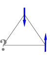
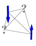
Figure 1.1: Triangular and tetrahedral frustrated units.

The kagome lattice is an example of a frustrated spin system with site-sharing triangular units, the pyrochlore lattice and its two-dimensional version, the pyrochlore checkerboard are examples with site-sharing tetrahedra (Fig. 1.2).

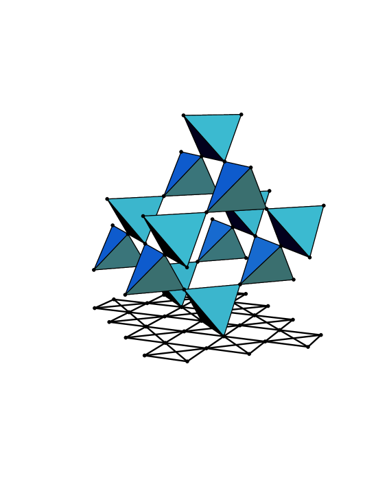
Figure 1.2: Pyrochlore lattice over checkerboard lattice.

Common to all these systems is the richness of classical ground states which make them very interesting but unfortunately also very hard to understand, especially in the quantum case. We were able to obtain some exact results (among the first in this field) for the fully frustrated quantum antiferromagnet on a pyrochlore checkerboard: With the help of the reflection symmetry of this two-dimensional lattice we have established rigorously that there is always a ground state with total spin zero (i.e., a singlet), furthermore, in the periodic case all ground states (if there is more than one) are singlets and the spin-expectation vanishes for each frustrated unit (this is the quantum analog of the “ice rule” for the corresponding Ising system). With the same methods we also found explicit upper bounds on the susceptibility, $\chi(T)\leq\frac{1}{8}$ (in natural units), both for the ground state and at finite temperature. This bound becomes exact in the classical high spin limit. The pyrochlore checkerboard is a system in which frustration effects are especially strong, so it is very exciting that a door to a more rigorous understanding of such systems has been opened.

Our approach combines old ideas of reflection positivity with more recent methods of Lieb and myself that we had originally tried to use with the Hubbard model (see chapter 3). Figure 1.3 illustrates the basic idea for the simpler case of a classical antiferromagnetic spin system:

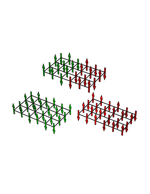
Figure 1.3: Reflection positivity for a classical antiferromagnet.

The lattice on the top shows a given state of the spin system, the two lattices on the bottom show derived states. They are constructed from the original state by reflecting the left (resp. right) half over to the right (resp. left) half while simultaneously flipping all the spins. This leads in either case to a state with a lower energy. (Recall that we are considering anti-ferromagnetic interaction.) If the original state was a ground state then the derived states must also be ground states of the system. In the quantum case things get more involved since states are in general superpositions of configurations like the ones in Figure 1.3. Mathematically the extra complexity can be handled by trace inequalities. Both in the classical and quantum case we gain a lot of useful information about ground states of such spin systems – the results mentioned above are some of the consequences. The method and some of the results generalize to other reflection symmetric lattices and hold in arbitrary dimensions. In section 1.2 we shall in particular establish the following exact properties of reflection symmetric spin systems with antiferromagnetic crossing bonds: At least one ground state has total spin zero and a positive semidefinite coefficient matrix and the crossing bonds obey an ice rule. This augments some previous results which were limited to bipartite spin systems and is of particular interest for frustrated spin systems.

There are many open questions and there is hope that much remains to be learned with the new approach which, by the way, has its origin in old work by Osterwalder on quantum field theory. This work was done in collaboration with E. Lieb at Princeton University and is published in [1, 2]. (The following two sections are based on these publications.)

1.1 The Pyrochlore checkerboard

1.1.1 Geometric frustration

Geometrically frustrated spin systems are known to have many interesting properties that are quite unlike those of conventional magnetic systems or spin glasses [12]. Most results are for classical systems. The first frustrated system, for which the richness of classical ground states was noted, was the triangular lattice [13]. Subsequently, the pyrochlore lattice, which consists of tetrahedra that share sites, was identified as a lattice on which the frustration effects are especially strong [14]. Unusual low-energy properties – in particular the absence of ordering at any temperature, was predicted both for discrete [14] and continuous [15] classical spin sytems. The ground state and low energy properties of the classical pyrochlore antiferromagnet – whose quantum version we are interested in – has been extensivly studied in [16]. Both the interest and difficulty in studying frustrated spin systems stem from the large ground-state degeneracy, which precludes most perturbative approaches.

As is the case for most other strong interacting systems in more than one dimension, very little is known exactly about the ground states of frustrated quantum spin systems. Most of the present knowledge has been obtained by numerics or clever approximations. Quantum fluctuations have been studied in the limits of large-$S$ [18], where a tendency towards lifting the ground-state degeneracy in favor of an ordered state (“quantum order by disorder”) was detected. In the opposite limit – $S=1/2$, where quantum fluctuations are much stronger – the pyrochlore antiferromagnet has been identified as a candidate for a quantum disordered magnet (“quantum spin liquid”) [19], and it has also been discussed in terms of a resonating valence bond approach [20]. However, there are no exact results against which to test the reliability of the results in this limit. In contrast to this, for conventional – bipartite – antiferromagnetic spin systems it is well known, for example, that the energy levels are ordered in a natural way according to spin, starting from spin zero [21]. Geometrically frustrated systems are not bipartite and thus this otherwise quite general theorem does not apply.

In the following we shall focus on the pyrochlore checkerboard: this is a two dimensional array of site-sharing tetrahedra, whose projection onto a plane is a square lattice with two extra diagonal bonds on every other square, see figures 1.2, 1.4(a). (The regular pyrochlore lattice is a three-dimensional array of site-sharing tetrahedra; it coincides with the checkerboard if suitable periodic boundary conditions are imposed.) The tetrahedra – or squares with extra diagonal bonds – are the frustrated units and will henceforth be called boxes.

Figure 1.4: (a) pyrochlore checkerboard, reflection symmetric about dashed line (b) frustrated unit with crossing bonds

The hamiltonian of a quantum Heisenberg antiferromagnet on a general lattice is (in natural units)

$$H_{\mbox{\tiny AF}}=\sum_{\langle i,j\rangle}{\bf s_{i}}\cdot{\bf s_{j}},$$ (1.1)

where the sum is over bonds $\langle i,j\rangle$ that connect sites $i$ and $j$ and ${\bf s}=(s^{1},s^{2},s^{3})$ are spin operators in the spin-$s$ representation, where $s$ can be anything. For the checkerboard lattice the hamiltonian is up to a constant equal to half the sum of the total spin squared of all boxes (labelled by $x$)

$$H=\frac{1}{2}\sum_{x}({\bf s_{1}}+{\bf s_{2}}+{\bf s_{3}}+{\bf s_{4}})_{x}^{2}.$$ (1.2)

A 3 $\times$ 3 checkerboard with periodic boundary conditions, i.e., with four independent sites, provides the simplest example. It has a hamiltonian that is (up to a constant) the total spin squared of one box and the energy levels, degeneracies, and eigenstates follow from the decomposition of the Hilbert space of four spin-$s$ particles into components of total spin; all ground states have total spin zero and there are $2s+1$ of them.

1.1.2 Reflection symmetry

A checkerboard lattice of arbitrary size, with or without periodic boundary conditions but with an even number of independent sites, has the property that it can be split into two equal parts that are mirror images of one another about a line that cuts bonds, as indicated in figure 1.4, and that contains no sites. We shall now show that such a system has at least one spin-zero ground state. It is actually not important, for the following argument, what the lattice looks like on the left or right; these sublattices neither need to be checkerboards nor do they have to be purely antiferromagnetic (as long as total spin is a good quantum number). What is impotant is, that the whole system is reflection symmetric about the line that separates left and right and that the crossing bonds are of checkerboard type. (For a system with periodic boundary conditions in one direction there will actually be two such lines, but we emphasize that periodic boundary conditions are not needed here even though it is needed in the usual reflection positivity applications; see [22] and references therein.) A key observation is that these crossing bonds (solid lines in figure 1.4(b)) form antiferromagnetic bonds $\bf S_{L}\cdot S_{R}$ between pairs of spins $\bf S_{L}=s_{1}+s_{2}$ and $\bf S_{R}=s_{3}+s_{4}$ of each box on the symmetry line.

The hamiltonian is $H=H_{L}+H_{R}+H_{C}$, where $H_{L}$ and $H_{R}$ act solely in the Hilbert spaces of the left, respectively right, subsystem and $H_{C}$ contains the crossing bonds. For the checkerboard $H_{C}=\sum_{y}(({\bf s_{1}+s_{2}})\cdot({\bf s_{3}+s_{4}}))_{y}$, with the sum over boxes $y$ that are bisected by the symmetry line. $H_{L}$ and $H_{R}$ are completely arbitrary as long as they commute with the total spin operator. We will, however, assume here that they are real in the $S^{3}$ basis. Any state of the system can be written in terms of a matrix $c$ as

$$\psi=\sum_{\alpha,\beta}c_{\alpha\beta}\psi^{L}_{\alpha}\otimes(\psi^{R}_{\beta})_{\mbox{\tiny rot}},$$ (1.3)

where the $\psi^{L}_{\alpha}$ form a real orthonormal basis of $S^{3}$ eigenstates for the left subsystem and the $(\psi^{R}_{\beta})_{\mbox{\tiny rot}}$ are the corresponding states for the right subsystem, but rotated by an angle $\pi$ around the 2-direction in spin space. This rotation takes $\uparrow$ into $\downarrow$, $\downarrow$ into $-\uparrow$, and more generally $|s,m\rangle$ into $(-)^{s-m}|s,-m\rangle$. It reverses the signs of the operators $S^{1}$ and $S^{3}$, while it keeps $S^{2}$ unchanged. The eigenvalue problem $H\psi=E\psi$ is now a matrix equation

$$h_{L}c+c(h_{R})^{T}-\sum_{i=1}^{3}\sum_{y}t_{y}^{(i)}c(t_{y}^{(i)})^{T}=Ec,$$ (1.4)

where $(h_{L})_{\alpha\beta}$ and $(h_{R})_{\alpha\beta}$ are real, symmetric matrix elements of the corrosponding terms in the hamiltonian and the $t_{y}^{(i)}$ are the real matrices defined for the spin operators $\bf s_{1}$ and $\bf s_{2}$ in box $y$ by $t^{(1,3)}_{\alpha\beta}=\langle\psi_{\alpha}^{L}|s^{(1,3)}_{1}+s^{(1,3)}_{2}|\psi_{\beta}^{L}\rangle$ and $t^{(2)}_{\alpha\beta}=i\langle\psi_{\alpha}^{L}|s^{(2)}_{1}+s^{(2)}_{2}|\psi_{\beta}^{L}\rangle$. Note the overall minus sign of the crossing term in (1.4): replacing $\bf s_{1}+s_{2}$ by $\bf s_{3}+s_{4}$ and $\psi^{L}$ by $(\psi^{R})_{\mbox{\tiny rot}}$ gives a change of sign for directions 1 and 3, while the $i$ in the definition of $t^{(2)}$ gives the minus sign for direction 2.

Consider now the energy expectation in terms of $c$:

$$\langle\psi|H|\psi\rangle=\mbox{tr\,}cc^{\dagger}h_{L}+\mbox{tr\,}c^{\dagger}ch_{R}-\sum_{i,y}\mbox{tr\,}c^{\dagger}t_{y}^{(i)}c(t_{y}^{(i)})^{\dagger}.$$ (1.5)

Since $H$ is left-right symmetric and by assumption real, we find that for an eigenstate of $H$ with coefficient matrix $c$, there is also an eigenstate with matrix $c^{\dagger}$ and, by linearity, with $c+c^{\dagger}$ and $i(c-c^{\dagger})$. Without loss of generality we may, therefore, write eigenstates of $H$ in terms of Hermitean $c=c^{\dagger}$. We shall also take $\psi$ to be normalized: $\langle\psi|\psi\rangle=\mbox{tr\,}c^{\dagger}c=1$. Following [23], let us write the trace in the last term of (1.5) in the diagonal basis of $c$: $-\mbox{tr\,}c^{\dagger}t_{y}^{(i)}c(t_{y}^{(i)})^{\dagger}=-\sum_{k,l}c_{k}c_{l}|(t_{y}^{(i)})_{kl}|^{2}$. This expression clearly does not increase if we replace all the $c_{k}$ by their absolute values $|c_{k}|$, i.e., if we replace the matrix $c$ by the positive semidefinite matrix $|c|=\sqrt{c^{2}}$. The first two terms in (1.5) and the norm of $\psi$ remain unchanged under this operation. We conclude that if $c$ is a ground state than so is $|c|$. Since $c=c^{+}-c^{-}$ and $|c|=c^{+}+c^{-}$, with positive semidefinite (p.s.d.) $c^{+}$ and $c^{-}$, we may, in fact, chose a basis of ground states with p.s.d. coefficient matrices.

1.1.3 Singlets and magnetization

Next, we will show that the state $\psi_{0}$ with the unit matrix as coefficient matrix (in the $S^{3}$ eigenbasis) has total spin zero. Since the overlap of $\psi_{0}$ with a state with matrix $c$ is simply the trace of $c$, which is neccessarily non-zero for states with a p.s.d. matrix, and because spin is a good quantum number of the problem, this will imply that there is a least one ground state with total spin zero. First consider a spin-1/2 system. In the $S^{3}$ eigenbasis every site has then either spin up or down. The state with unit coefficient matrix is a tensor product of singlets on corresponding pairs of sites $i\in L$, $i^{\prime}\in R$ of the two sublattices (see Fig. 1.5):

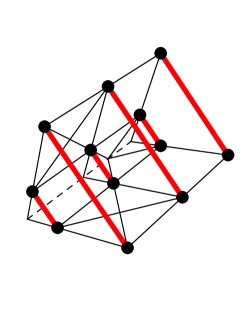
Figure 1.5: Canonical spin-zero state – the pyrochlore lattice is shown folded along the symmetry axis, thick lines represent singlets.

$$\psi_{0}=\bigotimes_{i\in L}\left(\uparrow(\uparrow)_{\mbox{\tiny rot}}+\downarrow(\downarrow)_{\mbox{\tiny rot}}\right)_{ii^{\prime}}=\bigotimes_{i\in L}\left(\uparrow\downarrow-\downarrow\uparrow\right)_{ii^{\prime}}.$$ (1.6)

The analogous state for a system with arbitrary spins,

$$\psi_{0}=\bigotimes_{i\in L}\sum_{m=-s}^{s}\left((-)^{s-m}|s,m\rangle\otimes|s,-m\rangle\right)_{ii^{\prime}},$$ (1.7)

is also a tensor product of spin-zero states.

Finally, we would like to show that the projection onto the spin zero part of a state with p.s.d. coefficient matrix preserves its positivity. This is only of academic interest here, but it is non-trivial and may very well be important for other physical questions. To find the projection onto spin zero we need to decompose the whole Hilbert space into tensor products of the spin components $[j]_{k}\otimes[j^{\prime}]_{k^{\prime}}$ of the two subsystems; here $k$, $k^{\prime}$ are additional quantum numbers that distinguish multiple multiplets with the same spin $j$. Only tensor products with $j=j^{\prime}$ can have a spin zero subspace, which is unique, in fact, and generated by the spin zero state $\displaystyle\sum_{m=-j}^{j}|j,m,k\rangle\otimes(-)^{j-m}|j,-m,k^{\prime}\rangle$. Noting that $(-)^{j-m}|j,-m,k^{\prime}\rangle$ is precisely the spin-rotated state $(|j,m,k^{\prime}\rangle)_{\mbox{\tiny rot}}$, we convince ourselves that the projection onto spin zero amounts to a partial trace over $m$ in a suitably parametrized matrix $c$. This operation preserves positive semidefiniteness, so we actually proved that the checkerboard has at least one ground state that has both total spin zero and a p.s.d. coefficient matrix $c$.

We do not know how many ground states there are. To determine the spin of any remaining ground states we add an external field to the hamiltonian and study the resulting magnetization. We will see that the spontaneous magnetization of every box on the symmetry line vanishes for all ground states, and thus if we have periodic boundary conditions in at least one direction, the total magnetization vanishes. Since $S^{3}_{\mbox{\tiny tot}}$ is a good quantum number and $S^{\pm}_{\mbox{\tiny tot}}$ commute with the hamiltonian, this will imply that all ground states in such a system have total spin zero. Let us thus modify the original hamiltonian (1.2) by replacing the term $(s_{1}^{(3)}+s_{2}^{(3)}+s_{3}^{(3)}+s_{4}^{(3)})^{2}_{z}$ for a single box, $z$, on the symmetry line by $(s_{1}^{(3)}+s_{2}^{(3)}+s_{3}^{(3)}+s_{4}^{(3)}-b)^{2}_{z}$, i.e., effectively adding a field $b$ to the spins in box $z$ and a constant term $\frac{1}{2}b^{2}$ to the hamiltonian. We want to distribute the resulting $b$-terms $(s_{1}^{(3)}+s_{2}^{(3)}-b/2)^{2}$, $(s_{3}^{(3)}+s_{4}^{(3)}-b/2)^{2}$, and $2(s_{1}^{(3)}+s_{2}^{(3)}-b/2)(s_{3}^{(3)}+s_{4}^{(3)}-b/2)$ to $H_{L}$, $H_{R}$, $H_{C}$ respectively. We cannot use the spin rotation as before, because the crossing terms in the hamiltonian would no longer be left-right symmetric in the basis (1.3). To avoid this problem we will, instead, expand eigenstates $\psi$ in the same basis on the left and on the right:

$$\psi=\sum_{\alpha,\beta}\tilde{c}_{\alpha\beta}\psi^{L}_{\alpha}\otimes\psi^{R}_{\beta}.$$ (1.8)

In this basis the hamiltonian is left-right symmetric and we may assume, as before, that $\tilde{c}=\tilde{c}^{\dagger}$. Except for the presence of $b$ in box $z$ the energy expectations on the left and right are as before. The energy expectation of the crossing terms of box $z$ in the diagonal basis of $\tilde{c}$ is now

$$\sum_{k,l}\tilde{c}_{k}\tilde{c}_{l}\left(|(t_{z}^{(1)})_{kl}|^{2}-|(t_{z}^{(2)})_{kl}|^{2}+|(t_{z}^{(3)})_{kl}-b/2|^{2}\right).$$

This expression clearly does not increase if we replace the $c_{k}$ by their absolute value $|c_{k}|$ and change the signs of the first and last terms. The sign change can be achieved by simultaneously performing a spin rotation and changing the sign of the field $b$ in the right subsystem. This actually completly removes $b$ from the hamiltonian. We have thus shown that the ground state energies of the systems $H_{b}$ with and $H_{0}$ without the $b$-terms satisfy the inequality $E_{b}\geq E_{0}$. Let $|b\rangle$ be a ground state of $H_{b}$ and $|0\rangle$ a ground state of $H_{0}$. It follows from the variational principle, that $\langle 0|H_{b}|0\rangle\geq\langle b|H_{b}|b\rangle=E_{b}\geq E_{0}$. Expressed in terms of spin operators this reads $E_{0}-2\langle 0|b(s_{1}^{(3)}+s_{2}^{(3)}+s_{3}^{(3)}+s_{4}^{(3)})_{z}|0\rangle+b^{2}\geq E_{0}$. Recalling that we are free to choose both the sign and the magnitude of $b$ we find that the ground state magnetization of box $z$ must be zero:

$$\langle 0|(s_{1}^{(3)}+s_{2}^{(3)}+s_{3}^{(3)}+s_{4}^{(3)})_{z}|0\rangle=0.$$ (1.9)

This quantum analog of the “ice rule” is true for any box on the symmetry line and it holds for all three spin components. In a system with periodic boundary conditions and an even number of sites in at least one direction we can choose the symmetry line(s) to intersect any given box, so in such a system the magnetization is zero both for every single box separately and also for the whole system: $\langle 0|S^{(3)}_{\mbox{\tiny tot}}|0\rangle=0$. As mentioned previously this implies that the total spin is zero for all ground states of such a system.

1.1.4 Susceptibility

Let us return to the inequality $E_{b}\geq E_{0}$. It implies a bound on the local susceptibility of the system: Let $E(b)\equiv\langle b|H_{0}-bS^{(3)}_{\mbox{\tiny box}}|b\rangle$ be the ground state energy of the periodic pyrochlore checkerboard with a single box immersed in an external field $b$. Recalling $H_{b}=H_{0}-bS^{(3)}_{\mbox{\tiny box}}+\frac{1}{2}b^{2}$, we see that the above inequality becomes $E(b)+\frac{1}{2}b^{2}\geq E(0)$ and, assuming differentiability, implies an upper bound on the susceptibility at zero field for single-box magnetization

$$\chi_{\mbox{\tiny loc}}=-\frac{1}{\lambda}\left.\frac{\partial^{2}E(b)}{\partial b^{2}}\right|_{b=0}\leq\frac{1}{4},$$ (1.10)

where $\lambda=4$ is the number of spins in a box. (The susceptibility is given in natural units in which we have absorbed the g-factor and Bohr magneton in the definition of the field $b$.)

We would like to get more detailed information about the response of the spin system to a global field $\{b_{x}\}$ in a hamiltonian $H_{\{b_{x}\}}$ which is identical to (1.2), except for the terms for the third spin component, which are replaced by $(s_{1}^{(3)}+s_{2}^{(3)}+s_{3}^{(3)}+s_{4}^{(3)}-b_{x})_{x}^{2}$. From what we have seen so far, it is apparent that the corresponding ground state energy $E_{\{b_{x}\}}$ is extremal for $b_{x}=0$. With the help of a more sophisticated trace inequality [25, 2], that becomes relevant whenever the matrix $c$ in (1.3) cannot be diagonalized, one can actually show that $E_{\{b_{x}\}}$ has an absolute minimum at $b_{x}=0$:

$$E_{\{b_{x}\}}\geq E_{0}.$$ (1.11)

Note that we had to put the field on the boxes for this result to hold; not every field on the individual spins can be written this way. The special choice $b_{x}=B/2$ corresponds to a global homogenous field $B$ on all spins. (The factor $1/2$ adjusts for the fact that every spin is shared by two boxes.) If $E(B)=\langle B|H_{0}-BS^{(3)}_{\mbox{\tiny tot}}|B\rangle$ is the ground state energy of the periodic pyrochlore checkerboard in the external field $B$, then (1.11) implies $E(B)+\frac{\Lambda}{16}B^{2}\geq E(0)$, and thus an upper bound on the susceptibility per site at zero field (in natural units)

$$\chi=-\frac{1}{\Lambda}\left.\frac{\partial^{2}E(B)}{\partial B^{2}}\right|_{B=0}\leq\frac{1}{8},$$ (1.12)

where $\Lambda$ is the number of independent sites, which equals twice the number of boxes.

All these results continue to hold at finite temperature. The analog of (1.11) holds also for the partition function corresponding to $H_{\{b_{x}\}}$:

$$Z_{\{b_{x}\}}\leq Z_{0},$$ (1.13)

as can be shown by a straightforward application of lemma 4.1 in section 4 of [22] to the pyrochlore checkerboard. The physically relevant partition function for the periodic pyrochlore checkerboard at finite temperature in a homogenous external field, $Z(B)\equiv\mbox{tr\,}e^{-\beta(H_{0}-BS^{(3)}_{\mbox{\tiny tot}})}$, differs from $Z_{\{b_{x}\}}$, where $b_{x}=B/2$, only by a factor corresponding to the constant term in $H_{\{b_{x}\}}$. Due to (1.13), the free energy $F(B)=-\beta^{-1}\ln Z(B)$ satisfies

$$F(B)+\frac{\Lambda}{16}B^{2}\geq F(0).$$ (1.14)

This implies (i) that the magnetization at zero field is still zero at finite temperature,

$$M_{T}=-\frac{1}{\Lambda}\left.\frac{\partial F(B)}{\partial B}\right|_{B=0}=0,$$ (1.15)

and, more interestingly, (ii) the same upper bound for the susceptibility per site at zero field as we had for the ground state:

$$\chi_{T}=-\frac{1}{\Lambda}\left.\frac{\partial^{2}F(B)}{\partial B^{2}}\right|_{B=0}\leq\frac{1}{8}.$$ (1.16)

The bounds on the susceptibility hold for arbitrary intrinsic spin-$s$ and agree very well with the results of [24] for the classical pyrochlore antiferromagnet in the un-diluted case.

It is not essential for our method that only every other square of the pyrochlore checkerboard is a frustrated unit, only the reflection symmmetry and the antiferromagnetic crossing bonds are important. We could, e.g., have diagonal bonds on every square, but then the horizontal and/or vertical bonds must have twice the coupling strength. Our results also apply to various 3-dimensional cubic versions of the checkerboard, e.g., with diagonal crossing bonds in every other cube, see figure 1.6.

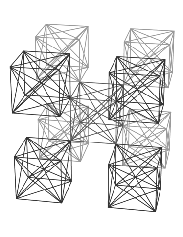
Figure 1.6: A 3-dimensional checkerboard: Every cube has 8 vertices – each shared among two cubes. This lattice exhibits even stronger frustration than the pyrochlore checkerboard. The expectation value of the total spin vector of each cube is zero, all ground states are singlets, the susceptibility is bounded above by 1/16.

While the method does not directly work for the 3D pyrochlore lattice because its geometry is too complicated, it has been seen in [16] that classically this system has similar properties to the pyrochlore checkerboard, which is also fully frustrated, and has the added advantage of being more easily visualizeable.

1.2 Singlets in reflection symmetric spin systems

1.2.1 Ordering energy levels according to spin

Total spin is often a useful quantum number to classify energy eigenstates of spin systems. An example is the antiferromagnetic Heisenberg Hamiltonian on a bipartite lattice, whose energy levels plotted versus total spin form towers of states. The spin-zero tower extends furthest down the energy scale, the spin-one tower has the next higher base, and so on, all the way up the spin ladder: $E(S+1)>E(S)$, where $E(S)$ denotes the lowest energy eigenvalue for total spin $S$ [21]. The ground state, in particular, has total spin zero; it is a singlet. This fact had been suspected for a long time, but the first rigorous proof was probably given by Marshall [26] for a one-dimensional antiferromagnetic chain with an even number of sites, each with intrinsic spin-1/2 and with periodic boundary conditions. This system is bipartite, it can be split into two subsystems, each of which contains only every other site, so that all antiferromagnet bonds are between these subsystems. Marshall bases his proof on a theorem that he attributes to Peierls: Any ground state of the system, expanded in terms of $S^{(3)}$-eigenstates has coefficients with alternating signs that depend on the $S^{(3)}$-eigenvalue of one of the subsystems. After a canonical transformation, consisting of a rotation of one of the subsystems by $\pi$ around the 2-axis in spin space, the theorem simply states that all coefficients of a ground state can be chosen to be positive. To show that this implies zero total spin, Marshall works in a subspace with $S^{(3)}$-eigenvalue $M=0$ and uses translation invariance. His argument easily generalizes to higher dimensions and higher intrinsic spin. Lieb, Schultz and Mattis [27] point out that translational invariance is not really necessary, only reflection symmetry is needed to relate the two subsystems, and the ground state is unique in the connected case. Lieb and Mattis [21] ultimately remove the requirement of translation invariance or reflection symmetry and apply the $M$-subspace method to classify excited states. Like Peierls they use a Perron-Frobenius type argument to prove that in the $S^{(3)}$-basis the ground state wave function for the connected case is a positive vector and it is unique. Comparing this wave function with the positive wave function of a simple soluble model in an appropriate $M$-subspace [23] they conclude that the ground state has total spin $S=|S_{A}-S_{B}|$, where $S_{A}$ and $S_{B}$ are the maximum possible spins of the two subsystems. (In the antiferromagnetic case $S_{A}=S_{B}$ and the ground state has total spin zero.) We shall now reintroduce reflection symmetry, but for other reasons: we want to exploit methods and ideas of “reflection positivity” (see [22] and references therein.) We do not require bipartiteness. The main application is to frustrated spin systems similar to the pyrochlore lattices discussed in the previous section.

1.2.2 Reflection symmetric spin system

We would like to consider a spin system that consists of two subsystems that are mirror images of one another, except for a rotation by $\pi$ around the 2-axis in spin-space, and that has antiferromagnetic crossing bonds between corresponding sets of sites of the two subsystems. The spin Hamiltonian is

$$H=H_{L}+H_{R}+H_{C},$$ (1.17)

and it acts on a tensor product of two identical copies of a Hilbert space that carries a representation of SU(2). “$H_{L}=\tilde{H}_{R}$” in the sense that $H_{L}=h\otimes 1$ and $H_{R}=1\otimes\tilde{h}$, where the tilde shall henceforth denote the rotation by $\pi$ around the 2-axis in spin-space. We make no further assumptions about the nature of $H_{L}$ and $H_{R}$, in particular we do not assume that these subsystems are antiferromagnetic. The crossing bonds are of anti-ferromagnetic type in the sense that $H_{C}=\sum_{A}\vec{S}_{A}\cdot\vec{S}_{A^{\prime}}$, with $\vec{S}_{A}=\sum_{i\in A}j_{i}\,\vec{s}_{i}$ and $\vec{S}_{A^{\prime}}=\sum_{i^{\prime}\in A^{\prime}}j_{i}\,\vec{s}_{i^{\prime}}$, where $A$ is a set of sites in the left subsystem, $A^{\prime}$ is the corresponding set of sites in the right subsystem, and $j_{i}$ are real coefficients. The intrinsic spins $s_{i}$ are arbitrary and can vary from site to site, as long as the whole system is reflection symmetric. We shall state explicitly when we make further assumptions, e.g., that the whole system is invariant under spin-rotations.

Figure 1.7: Some possible crossing bonds.

Any state of the system can be expanded in terms of a square matrix $c$,

$$\psi=\sum_{\alpha,\beta}c_{\alpha\beta}\psi_{\alpha}\otimes\widetilde{\psi}_{\beta},$$ (1.18)

where $\{\psi_{\alpha}\}$ is a basis of $S^{(3)}$-eigenstates. (The indices $\alpha$, $\beta$ may contain additional non-spin quantum numbers, as needed, and the tilde on the second tensor factor denotes the spin rotation.) We shall assume that the state is normalized: $\langle\psi|\psi\rangle=\mbox{tr\,}cc^{\dagger}=1$. The energy expectation in terms of $c$ is a matrix expression

$$\langle\psi|H|\psi\rangle=\mbox{tr\,}cc^{\dagger}h+\mbox{tr\,}(c^{\dagger}c)^{T}h-\sum_{A}\sum_{a=1}^{3}\mbox{tr\,}c^{\dagger}S_{A}^{(a)}c(S_{A}^{(a)})^{\dagger},$$ (1.19)

here $(h)_{\alpha\beta}=\langle\psi_{\alpha}|H_{L}|\psi_{\beta}\rangle=\langle\widetilde{\psi}_{\alpha}|H_{R}|\widetilde{\psi}_{\beta}\rangle$, $(S_{A}^{(a)})_{\alpha\beta}=\langle\psi_{\alpha}|\sum_{i\in A}j_{i}\,s^{(a)}_{i}|\psi_{\beta}\rangle$, and we have used $(\widetilde{S_{A}^{(a)}})^{T}=-(S_{A}^{(a)})^{\dagger}$. (For $a=1,3$ the minus sign comes from the spin rotation, for $a=2$ it comes from complex conjugation. This can be seen by writing $S^{(1)}$ and $S^{(2)}$ in terms of the real matrices $S^{+}$ and $S^{-}$.) Note, that we do not assume $(h)_{\alpha\beta}$ to be real or symmetric, otherwise the following considerations would simplify considerably [1].

We see, by inspection, that the energy expectation value remains unchanged if we replace $c$ by its transpose $c^{T}$, and, by linearity, if we replace it by $c+c^{T}$ or $c-c^{T}$. So, if $c$ corresponds to a ground state, then we might as well assume for convenience that $c$ is either symmetric or antisymmetric. Note, that in either case we have $(c_{R})^{T}=c_{L}$, where $c_{L}\equiv\sqrt{cc^{\dagger}}$ and $c_{R}\equiv\sqrt{c^{\dagger}c}$. (Proof: $(c_{R}^{2})^{T}=(c^{\dagger}c)^{T}=cc^{\dagger}=c_{L}^{2}$, if $c^{T}=\pm c$; now take the unique square root of this.) Using this we see that the first two terms in the energy expectation equal $2\mbox{tr\,}c_{L}^{2}h$ and thus depend on $c$ only through the positive semidefinite matrix $c_{L}$. With the help of a trace inequality we will show that the third term does not increase if we replace $c$ by the positive semidefinite matrix $c_{L}$.

1.2.3 Trace inequality

For any square matrices $c$, $M$, $N$ it is true that [25]

$$|\mbox{tr\,}c^{\dagger}McN^{\dagger}|\leq\frac{1}{2}\left(\mbox{tr\,}c_{L}Mc_{L}M^{\dagger}+\mbox{tr\,}c_{R}Nc_{R}N^{\dagger}\right),$$ (1.20)

where $c_{R}=\sqrt{c^{\dagger}c}$, $c_{L}=\sqrt{cc^{\dagger}}$ are the unique square roots of the positive semidefinite matrices $c^{\dagger}c$ and $cc^{\dagger}$. Here is a proof: By the polar decomposition theorem $c=uc_{R}$ with a unitary matrix $u$ and $(uc_{R}u^{\dagger})^{2}=uc^{\dagger}cu^{\dagger}=cc^{\dagger}=c_{L}^{2}$, so by the uniqueness of the square root $uc_{R}u^{\dagger}=c_{L}$. Similarly, for any function $f$ on the non-negative real line $uf(c_{R})u^{\dagger}$ = $f(c_{L})$, and in particular $u\sqrt{c_{R}}=\sqrt{c_{L}}u$ and thus $c=\sqrt{c_{L}}u\sqrt{c_{R}}$. Let $P\equiv u^{\dagger}\sqrt{c_{L}}M\sqrt{c_{L}}u$ and $Q\equiv\sqrt{c_{R}}N^{\dagger}\sqrt{c_{R}}$, then

$$|\mbox{tr\,}c^{\dagger}McN^{\dagger}| = |\mbox{tr\,}PQ|\,\leq\,\frac{1}{2}(\mbox{tr\,}PP^{\dagger}+\mbox{tr\,}QQ^{\dagger})$$ (1.21)

$$= \frac{1}{2}\left(\mbox{tr\,}c_{L}Mc_{L}M^{\dagger}+\mbox{tr\,}c_{R}Nc_{R}N^{\dagger}\right),$$

where the inequality is simply the geometric arithmetic mean inequality for matrices

$$|\mbox{tr\,}PQ|=|\sum_{i,j}P_{ij}Q_{ji}|\leq\frac{1}{2}\sum_{i,j}(|P_{ij}|^{2}+|Q_{ji}|^{2})=\frac{1}{2}(\mbox{tr\,}PP^{\dagger}+\mbox{tr\,}QQ^{\dagger}).$$

Spin rings – with or without reflection symmetry

Inequality (1.20) also holds for rectangular matrices: If $c$ is an $m\times n$ matrix then $M$ and $N$ are $m\times m$ and $n\times n$-matrices respectively, $u$ is a partial isometry and $c_{L}$ and $c_{R}$ are positive $m\times m$ and $n\times n$ matrices respectively. This was originally of interest for the ordering of energy levels in the Hubbard model (see chapter 3) and for Bose-Einstein condensation in the hard core lattice approximation away from half-filling, but may also be used to find rigorous inequalities for the ground state energy of 1-dimensional periodic spin systems (spin rings) with an even or odd number of spins, as illustrated in figures 1.8 and 1.9.

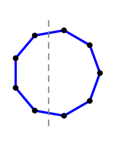
Figure 1.8: Ring with $n+m$ spins. Reflection along the dottet line leads to two rings with $2n$ and $2m$ spins respectively. The trace inequality and (1.19) imply an inequality for the ground state energies: $E_{n+m}\geq\frac{1}{2}(E_{2n}+E_{2m})$.

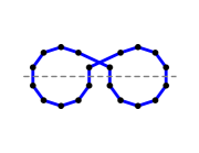
$\;\rightarrow$

$\,,$

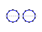
Figure 1.9: Figure-8 ring with $2n$ spins ($n$ even). Reflection along the dotted line leads to two pairs of rings with $n$ spins each. The trace inequality and (1.19) imply an inequality for the ground state energy per spin: $e_{2n}\geq e_{n}$.

1.2.4 Positive spin-zero ground state

Existence of a positive ground state

Consider any ground state of the system with coefficient matrix $c=\pm c^{T}$ and apply the trace inequality to the terms in $\langle\psi|H_{C}|\psi\rangle$:

$$-\mbox{tr\,}c^{\dagger}S_{A}^{(a)}c(S_{A}^{(a)})^{\dagger}\geq-\frac{1}{2}\left(\mbox{tr\,}c_{L}S_{A}^{(a)}c_{L}(S_{A}^{(a)})^{\dagger}+\mbox{tr\,}c_{R}S_{A}^{(a)}c_{R}(S_{A}^{(a)})^{\dagger}\right),$$

but $(c_{R}S_{A}^{(a)}c_{R}(S_{A}^{(a)})^{\dagger})^{T}=((S_{A}^{(a)})^{T})^{\dagger}c_{L}(S_{A}^{(a)})^{T}c_{L}=(S_{A}^{(a)})^{\dagger}c_{L}(S_{A}^{(a)})c_{L}$, so in fact

$$-\mbox{tr\,}c^{\dagger}S_{A}^{(a)}c(S_{A}^{(a)})^{\dagger}\geq-\mbox{tr\,}c_{L}S_{A}^{(a)}c_{L}(S_{A}^{(a)})^{\dagger}.$$

Since the normalization of the state and the other terms in (1.5) are unchanged if we replace $c$ by $c_{L}=\sqrt{cc^{\dagger}}$, and because we have assumed that $c$ is the coefficient matrix of a ground state, it follows that the positive semidefinite matrix $c_{L}$ must also be the coefficient matrix of a ground state.

Overlap with canonical spin zero state

Consider the (not normalized) canonical state with coefficient matrix given by the identity matrix in a basis of $S^{(3)}$-eigenstates of either subsystem

$$\Xi = \displaystyle\sum_{k,k^{\prime}}\sum_{j}\sum_{m=-j}^{j}\psi_{(j,m,k)}\otimes\widetilde{\psi}_{(j,m,k^{\prime})}$$ (1.22)

$$= \displaystyle\sum_{k,k^{\prime}}\sum_{j}\sum_{\tilde{m}=-j}^{j}\psi_{(j,m,k)}\otimes(-)^{j-m}\psi_{(j,-m,k^{\prime})}.$$

The states are labeled by the usual spin quantum numbers $j$, $m$ and an additional symbolic quantum number $k$ to lift remaining ambiguities. The state $\Xi$ has total spin zero because of the spin rotation in the right subsystem: Its $S_{\mbox{\tiny tot}}^{(3)}$-eigenvalue is zero and acting with either $S^{+}_{\mbox{\tiny tot}}$ or $S^{-}_{\mbox{\tiny tot}}$ on it gives zero. The overlap of any state with coefficient matrix $c$ with the canonical state $\Xi$ is simply the trace of $c$. In the previous section we found that the reflection symmetric spin system necessarily has a ground state with positive semidefinite, non-zero coefficient matrix, which, by definition, has a (non-zero) positive trace. Since the trace is proportional to the overlap with the canonical spin-zero state, we have now shown that there is always a ground state that contains a spin-zero part. Provided that total spin is a good quantum number, we can conclude further that our system always has a ground state with total spin zero, i.e., a singlet.

Projection onto spin zero

Consider any state $\psi=\sum c_{\alpha\beta}\psi_{\alpha}\otimes\widetilde{\psi}_{\beta}$ with positive semidefinite $c=|c|$. We have seen that this implies that $\psi$ has a spin-zero component. If total spin is a good quantum number it is interesting to ask what happens to $c$ when we project $\psi$ onto its spin zero part

$$\psi^{0}=\sum c^{0}_{\alpha\beta}\psi_{\alpha}\otimes\widetilde{\psi}_{\beta}.$$ (1.23)

We shall show that the coefficient matrix $c^{0}$ of $\psi^{0}$ is a partial trace of $c$ and thus still positive semidefinite. A convenient parametrisation of the $S^{3}$ eigenstates $\psi_{\alpha}$ for this task is, as before, $\alpha=(j,m,k)$, where $k$ labels spin-$j$ multiplets $[j]_{k}$ in the decomposition of the Hilbert space of one subsystem into components of total spin. Note that $[j]_{k}\otimes[j^{\prime}]_{k^{\prime}}=[j+j^{\prime}]\oplus\ldots\oplus[|j-j^{\prime}|]$, so $[j]_{k}\otimes[j^{\prime}]_{k^{\prime}}$ contains a spin zero subspace only if $j=j^{\prime}$, and for each $k$, $k^{\prime}$ that subspace is unique and generated by the normalized spin zero state

$$\xi_{k,k^{\prime}}=(2j+1)^{-\frac{1}{2}}\sum_{\tilde{m}=-j}^{j}\psi_{(j,\tilde{m},k)}\otimes\widetilde{\psi}_{(j,\tilde{m},k^{\prime})}.$$ (1.24)

(Recall that $\widetilde{\psi}_{(j,\tilde{m},k^{\prime})}=(-)^{j-\tilde{m}}\psi_{(j,-\tilde{m},k^{\prime})}$ is the rotation of $\psi_{(j,\tilde{m},k^{\prime})}$ by $\pi$ around the 2-axis in spin space.) The projection of $\psi$ onto spin zero is thus amounts to replacing $c$ with $c^{0}$, where

$$c^{0}_{(j,m,k)(j^{\prime},m^{\prime},k^{\prime})}=\left\{\begin{array}[]{l}0\quad\mbox{if $j\neq j^{\prime}$ or $m\neq m^{\prime}$}\\ \displaystyle\frac{N}{2j+1}\sum_{\tilde{m}=-j}^{j}c_{(j,\tilde{m},k)(j,\tilde{m},k^{\prime})}\quad\mbox{else}.\end{array}\right.$$ (1.25)

($N$ is a overall normalisation constant, independent of $j$, $m$, $k$.) Let us now show that this partial trace preserves positivity, i.e., $(v,c^{0}\;v)\geq 0$ for any vector $v=\left(v_{(j,m,k)}\right)$ of complex numbers. If we decompose $v$ into a sum of vectors $v_{jm}$ with definite $j$, $m$ and use (1.25), we see

$$(v,c^{0}\,v)=\sum_{j,m}(v_{jm},c^{0}\,v_{jm})=\sum_{j,m,\tilde{m}}(\omega_{j\tilde{m}}^{m},c\,\omega_{j\tilde{m}}^{m})\geq 0,$$ (1.26)

where the $\omega_{j\tilde{m}}^{m}$ are new vectors with components $\omega_{(j,\tilde{m},k)}^{m}=v_{(j,m,k)}$, independent of $\tilde{m}$. Every term in the last sum is non-negative because $c$ is positive semidefinite by assumption. This result implies in particular that a reflection symmetric spin system always has a ground state with total spin zero and positive semidefinite coefficient matrix – provided that total spin is a good quantum number.

1.2.5 Ice rule for crossing bonds

The expectation of the third spin component of the sites involved in each crossing bond $B$, weighted by their coefficients $j_{i}$, vanishes for any ground state $\psi_{0}$,

$$\langle\psi_{0}|\sum_{i\in B}j_{i}(s_{i}^{(3)}+s_{i^{\prime}}^{(3)})|\psi_{0}\rangle=0,$$ (1.27)

provided that either the left and right subsystems are invariant under the spin rotation, $h=\tilde{h}$, or that their matrix elements are real (the latter is equivalent to the assumption $h=h^{T}$, since we know that $h=h^{\dagger}$ or otherwise the whole spin Hamiltonian would not be Hermitean). By symmetry (1.27) will also be true for the first spin component and, if we are dealing with a spin Hamiltonian that is invariant under spin rotations, it is also true for the second spin component. For ground states with symmetric or antisymmetric coefficient matrix we automatically have $\langle s_{i}^{(3)}+s_{i^{\prime}}^{(3)}\rangle=0$ for any pair of sites $i$ and $i^{\prime}$, so in that case (1.27) is trivial.

For the proof we introduce a real parameter $b$ in the spin Hamiltonian: $H(b)\equiv H-b(S^{(3)}_{B}+S^{(3)}_{B^{\prime}})+b^{2}/2$, where $B$ is one of the sets of sites involved in the crossing bonds of the original Hamiltonian $H$. Let $E_{b}$ be the ground state energy of $H(b)$ and $E_{0}$ the ground state energy of $H$. One can show that $E_{b}\geq E_{0}$ and (1.27) follows then by a variational argument:

$$\langle\psi_{0}|H(b)|\psi_{0}\rangle\geq E_{b}\geq E_{0}=\langle\psi_{0}|H|\psi_{0}\rangle,$$ (1.28)

or, $\langle\psi_{0}|b(S^{(3)}_{B}+S^{(3)}_{B^{\prime}})|\psi_{0}\rangle\leq b^{2}/2$, which implies (1.27). Note, that we did not make any assumptions about the symmetry or antisymmetry of the coefficient matrix of $\psi_{0}$ here.

Sketch of the proof of $E_{b}\geq E_{0}$ (see also [25, 1]): $H(b)=H_{L}(b)+H_{R}(b)+H_{C}(b)+b^{2}/4$ with $H_{L,R}(b)=H_{L,R}-b/2\cdot S^{(3)}_{B}$ and $H_{C}(b)$ equal to $H_{C}$ except for the term $S^{(3)}_{B}\cdot S^{(3)}_{B^{\prime}}$, which is replaced by $(S^{(3)}_{B}-b/2)\cdot(S^{(3)}_{B^{\prime}}-b/2)$. If we now write the ground state energy expectation of $H(b)$ as a matrix expression like (1.5) and apply the trace inequality to it, we will find an equal or lower energy expectation not of $H(b)$, but rather of $H$: The trace inequality effectively removes the parameter $b$ from the Hamiltonian. By the variational principle the true ground state energy of $H$ is even lower and we conclude that $E_{b}\geq E_{0}$. Role of the technical assumptions mentioned above: If $h=h^{T}$, then the transpose in the second term in (1.5) vanishes, the matrix expression is symmetric in $c_{L}$ and $c_{R}$ (except for the sign of the parameter $b$), and the trace inequality gives $\langle H(b)\rangle_{c}\geq\frac{1}{2}\left\{\langle H\rangle_{c_{L}}+\langle H\rangle_{c_{R}}\right\}$. If $h=\tilde{h}$, then we should drop the spin rotation on the second term of the analog of expression (1.18) for $\psi_{b}$. The matrix expression for $\langle H(b)\rangle$ is then symmetric in $c$ and $c^{T}$ and we may assume $c=\pm c^{T}$ to prove $E_{b}\geq E_{0}$. The calculation is similar to the one in section 1.2.4. Note, that $c=\pm c^{T}$ only enters the proof of $E_{b}\geq E_{0}$, we still do not need to assume that the coefficient matrix of $\psi_{0}$ in (1.27) has that property.

The preferred configurations of four spins with antiferromagnetic crossed bonds in a classical Ising system are very similar to the configurations of the four hydrogen atoms that surround each oxygen atom in ice (Fig. 1.10):

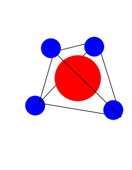
Figure 1.10: Pauli’s ice rule for hydrogen atoms around an oxigen atom: Two hydrogen atoms are closer to and two are further away from each oxygen atom. In the analogous Ising system this would correspond to the magnetic quantum number $M=0$. We have found such an ice rule for the spins involved in each crossing bond.

There are always two hydrogen atoms close and two further away from each oxygen atom, and there are always two spins “up” and two “down”, i.e. $M=0$, in the Ising system. Equation $(\ref{ice})$ is a (generalized) quantum mechanical version of this – that is why we use the term “ice rule”. This phrase is also used in the context of ferromagnetic pyrochlore with Ising anisotropy (“spin ice”) [28] and we hope that does not cause confusion.

1.2.6 Comparison with previous results

We would like to discuss similarities between our method and previous work, in particular the approach of [21] for the bipartite antiferromagnet: There, the spin Hamiltonian splits into two parts $H=H_{0}+H_{1}$. The expectation value of $H_{0}$ with respect to a state $\psi=\sum f_{\alpha}\phi_{\alpha}$, expanded in an appropriate basis $\{\phi_{\alpha}\}$, depends only on $|f_{\alpha}|$, and the expectation of $H_{1}$ does not increase under the transformation $f_{\alpha}\rightarrow|f_{\alpha}|$. The variational principle then implies that there must be a ground state with only non-negative coefficients $|f_{\alpha}|$. The present setup is very similar, except that we use coefficient matrices $(c_{\alpha\beta})$ to expand states, since we work on a tensor product of Hilbert spaces. In our case the expectation value of $H_{0}=H_{L}+H_{R}$ depends only on $c$ via the positive matrices $c_{L}$ and $c_{R}$, and the expectation value of $H_{C}$ increases if we “replace” $c$ by these positive matrices. The similarity is even more apparent if $h$ has real matrix elements: In that case we may assume that $c$ is diagonalisable and its eigenvalues play the role of the coefficients $f_{\alpha}$. The spin of a positive ground state is established in all cases from the overlap with a state of known spin that is also positive. In a system with sufficient symmetry we can, however, also use the “ice rule” to prove that all ground states have total spin zero [1]. (E.g., in a system with constant coefficients $j_{i}$ and enough translational invariance, so that every spin can be considered to be involved in a crossing bond and thus in an ice rule, we would conclude that all ground states have $S^{(3)}_{\mbox{\tiny tot}}=0$ and, assuming rotational invariance in spin space, $S_{\mbox{\tiny tot}}=0$.) It is not clear, if $M$-subspace methods can be used in the present setting to get information about excited states. An important point in the our work is that we consider not only antiferromagnetic bonds between single sites but also bonds between sets of sites. This frees us from the requirement of bipartiteness and even allows some ferromagnetic crossing bonds, for example in $(s_{1}-s_{2})(s_{1^{\prime}}-s_{2^{\prime}})$. There is no doubt that the scheme can be further generalized, e.g., to other groups or more abstract “crossing bonds”. In the present form the most interesting applications are in the field of frustrated spin systems [1].

We did not address the question of the degeneracy of ground states. Classically a characteristic feature of frustrated systems is their large ground state degeneracy. For frustrated quantum spin systems this is an important open problem.

Chapter 2 Wehrl entropy of Bloch coherent states

There is a hybrid between the quantum mechanical entropy, $-\mbox{tr}\rho\ln\rho$, and the entropy of the corresponding classical system: Wehrl proposed to use the expectation $\langle z|\rho|z\rangle$ of the density matrix between coherent states as probability density for the Shannon entropy; $S_{W}=-\int dz\;\langle z|\rho|z\rangle\ln\langle z|\rho|z\rangle$. It turns out that this entropy has nice properties, some of which either of its ‘parents’ lack: The Wehrl entropy is sub-additive, monotone and always positive – even for pure states. In fact, it is always larger than the quantum entropy.

Wehrl conjectured that the minimum of $S_{W}$ for a single particle on the line is reached only for density matrices that are projectors onto coherent states. This was proved by Lieb using advanced theorems in Fourier analysis. While it is well-known that entropy considerations can lead to non-trivial inequalities (they e.g. improve on Heisenberg’s uncertainty), it was still quite surprising that the proof of Wehrl’s conjecture was so hard. In an effort to shed more light on this, Lieb was led to a related conjecture for Bloch coherent states. Even though many attempts have been made to find a proof of the latter, there had been virtually no progress for the last twenty years. Using a geometric representation of spin states we will see in the following sections how to compute the Wehrl entropy explicitly and will settle the conjecture for cases of low spin. We will also give a group theoretic proof for all spin of a related inequality.

Sharp inequalities that stem from entropy considerations have in the past been seen to be very useful in mathematical physics. In this particular case there is a way to use Lieb’s conjecture to get much better approximations to probability distributions than are in use today. There is also a direct physical interpretation: The Wehrl Entropy for states of spin $j$ is the entropy of a point vortex on the sphere in the background of $2j$ fixed point vortices with the usual vortex-interaction. We find that a proof of Lieb’s conjecture for low spins can be reduced to some beautiful spherical geometry, but the unreasonable difficulty of a complete proof is still a great puzzle; its resolution may very well lead to interesting mathematics and perhaps physics.

The results have been published in [3], the remainder of this chapter is based on that publication. Much of the early work was done in collaboration with Wolfgang Spitzer who

2.1 Conjectures of Wehrl and Lieb

For a quantum mechanical system with density matrix $\rho$, Hilbert space ${\cal H}$, and a family of normalized coherent states $|z\rangle$, parametrized symbolically by $z$ and satisfying $\int dz\,|z\rangle\langle z|={\bf 1}$ (resolution of identity), the Wehrl entropy [44] is

$$S_{W}(\rho)=-\int dz\,\langle z|\rho|z\rangle\ln\langle z|\rho|z\rangle,$$ (2.1)

i.e., this new entropy is the ordinary Shannon entropy of the probability density provided by the lower symbol of the density matrix. If we are dealing with a tensor product ${\cal H}_{1}\otimes{\cal H}_{2}$ of Hilbert spaces we can either consider the total entropy $S_{12}$ directly, or we can use partial traces to compute reduced density matrices $\rho_{1}$, $\rho_{2}$ and the associated entropies $S_{1}$ and $S_{2}$. It would be physically desirable to have inequalities

$$S_{1}\leq S_{12}\leq S_{1}+S_{2}$$ (2.2)

but it turns out that while subadditivity $S_{12}\leq S_{1}+S_{2}$ is no problem, monotonicity $S_{1}\leq S_{1}+S_{2}$ in general fails for quantum entropy and for classical continuous entropy. For the Wehrl entropy, however, both inequalities are valid. Furthermore it also satisfies concavity in $\rho$ and strong subadditivity [35, 36].

Like quantum mechanical entropy, $S_{Q}=-\mbox{tr\,}\rho\ln\rho$, Wehrl entropy is always non-negative, in fact $S_{W}>S_{Q}\geq 0$. In view of this inequality it is interesting to ask for the minimum of $S_{W}$ and the corresponding minimizing density matrix. It follows from concavity of $-x\ln x$ that a minimizing density matrix must be a pure state, i.e., $\rho=|\psi\rangle\langle\psi|$ for a normalized vector $|\psi\rangle\in{\cal H}$ [34]. (Note that $S_{W}(|\psi\rangle\langle\psi|)$ depends on $|\psi\rangle$ and is non-zero, unlike the quantum entropy which is of course zero for pure states.)

For Glauber coherent states Wehrl conjectured [44] and Lieb proved [34] that the minimizing state $|\psi\rangle$ is again a coherent state. It turns out that all Glauber coherent states have Wehrl entropy one, so Wehrl’s conjecture can be written as follows:

Theorem 2.1.1 (Lieb)

The minimum of $S_{W}(\rho)$ for states in ${\cal H}=L^{2}(\mathbb{R})$ is one,

$$S_{W}(|\psi\rangle\langle\psi|)=-\int dz\,|\langle\psi|z\rangle|^{2}\ln|\langle\psi|z\rangle|^{2}\geq 1,$$ (2.3)

with equality if and only if $|\psi\rangle$ is a coherent state.

To prove this, Lieb used a clever combination of the sharp Hausdorff-Young inequality [30, 37, 39] and the sharp Young inequality [31, 30, 37, 39] to show that

$$s\int dz\,|\langle z|\psi\rangle|^{2s}\leq 1,\quad s\geq 1,$$ (2.4)

again with equality if and only if $|\psi\rangle$ is a coherent state. Wehrl’s conjecture follows from this in the limit $s\rightarrow 1$ essentially because (2.3) is the derivative of (2.4) with respect to $s$ at $s=1$. All this easily generalizes to $L^{2}(\mathbb{R}^{n})$ [34, 38].

The lower bound on the Wehrl entropy is related to Heisenberg’s uncertainty principle [29, 32] and it has been speculated that $S_{W}$ can be used to measure uncertainty due to both quantum and thermal fluctuations [32].

It is very surprising that ‘heavy artillery’ like the sharp constants in the mentioned inequalities are needed in Lieb’s proof. To elucidate this situation, Lieb suggested [34] studying the analog of Wehrl’s conjecture for Bloch coherent states $|\Omega\rangle$, where one should expect significant simplification since these are finite dimensional Hilbert spaces. However, no progress has been made, not even for a single spin, even though many attempts have been made [35]. Attempts to proceed again along the lines of Lieb’s original proof have failed to provide a sharp inequality and the direct computation of the entropy and related integrals, even numerically, was unsuccessful [42].

The key idea turns out to be a geometric representation of a state of spin $j$ as $2j$ points on a sphere. In this representation the expression $|\langle\Omega|\psi\rangle|^{2}$ factorizes into a product of $2j$ functions $f_{i}$ on the sphere, which measure the square chordal distance from the antipode of the point parametrized by $\Omega$ to each of the $2j$ points on the sphere. Lieb’s conjecture, in a generalized form analogous to (2.4), then looks like the quotient of two Hölder inequalities

$$\frac{|\!|f_{1}\cdots f_{2j}|\!|_{s}}{|\!|f_{1}\cdots f_{2j}|\!|_{1}}\leq\frac{\prod_{i=1}^{2j}|\!|f_{i}|\!|_{2js}}{\prod_{i=1}^{2j}|\!|f_{i}|\!|_{2j}},$$ (2.5)

with the one with the higher power winning against the other one. We shall give a group theoretic proof of this inequality for the special case $s\in\mathbb{N}$ in theorem 2.2.8.

In the geometric representation the Wehrl entropy of spin states finds a direct physical interpretation: It is the classical entropy of a single particle on a sphere interacting via Coulomb potential with $2j$ fixed sources; $s$ plays the role of inverse temperature.

The entropy integral (2.1) can now be done because $|\langle\Omega|\psi\rangle|^{2}$ factorizes and one finds a formula for the Wehrl entropy of any state. When we evaluate the entropy explicitly for states of spin 1, 3/2, and 2 we find surprisingly simple expressions solely in terms of the square chordal distances between the points on the sphere that define the given state.

A different, more group theoretic approach seems to point to a connection between Lieb’s conjecture and the norm of certain spin $js$ states with $1\leq s\in\mathbb{R}$ [33]. So far, however, this has only been useful for proving the analog of inequality (2.4) for $s\in\mathbb{N}$.

2.1.1 Bloch coherent spin states

Glauber coherent states

$$|z\rangle=\pi^{-\frac{1}{4}}e^{-(x-q)^{2}/2}e^{ipx},$$ (2.6)

parametrized by $z=(q+ip)/\sqrt{2}$ and equiped with a measure $dz=dpdq/2\pi$, are usually introduced as eigenvectors of the annihilation operator $a=(\hat{x}+i\hat{p})/\sqrt{2}$, $a|z\rangle=z|z\rangle$, but the same states can also be obtained by the action of the Heisenberg-Weyl group $H_{4}=\{a^{\dagger}a,a^{\dagger},a,I\}$ on the extremal state $|0\rangle=\pi^{-\frac{1}{4}}e^{-x^{2}/2}$. Glauber coherent states are thus elements of the coset space of the Heisenberg-Weyl group modulo the stability subgroup $U(1)\otimes U(1)$ that leaves the extremal state invariant. (See e.g. [45] and references therein.) This construction easily generalizes to other groups, in particular to SU(2), where it gives the Bloch coherent spin states [41] that we are interested in: Here the Hilbert space can be any one of the finite dimensional spin-$j$ representations $[j]\equiv\mathbb{C}^{2j+1}$ of SU(2), $j={1\over 2},1,\frac{3}{2},\ldots$, and the extremal state for each $[j]$ is the highest weight vector $|j,j\rangle$. The stability subgroup is U(1) and the coherent states are thus elements of the sphere $S_{2}=$SU(2)/U(1); they can be labeled by $\Omega=(\theta,\phi)$ and are obtained from $|j,j\rangle$ by rotation:

$$|\Omega\rangle_{j}={\cal R}_{j}(\Omega)|j,j\rangle.$$ (2.7)

For spin $j=\frac{1}{2}$ we find

$$|\omega\rangle=p^{\frac{1}{2}}e^{-i{\phi\over 2}}|\!\uparrow\rangle+(1-p)^{\frac{1}{2}}e^{i{\phi\over 2}}|\!\downarrow\rangle,$$ (2.8)

with $p\equiv\cos^{2}\frac{\theta}{2}$. (Here and in the following $|\omega\rangle$ is short for the spin-$\frac{1}{2}$ coherent state $|\Omega\rangle_{\frac{1}{2}}$; $\omega=\Omega=(\theta,\phi)$. $|\!\uparrow\rangle\equiv|\frac{1}{2},\frac{1}{2}\rangle$ and $|\!\downarrow\rangle\equiv|\frac{1}{2},-\frac{1}{2}\rangle$.) An important observation for what follows is that the product of two coherent states for the same $\Omega$ is again a coherent state:

$$|\Omega\rangle_{j}\otimes|\Omega\rangle_{j^{\prime}} = ({\cal R}_{j}\otimes{\cal R}_{j^{\prime}})\,(|j,j\rangle\otimes|j^{\prime},j^{\prime}\rangle)$$ (2.9)

$$= {\cal R}_{j+j^{\prime}}\,|j+j^{\prime},j+j^{\prime}\rangle\;=\;|\Omega\rangle_{j+j^{\prime}}.$$

Coherent states are in fact the only states for which the product of a spin-$j$ state with a spin-$j^{\prime}$ state is a spin-$(j+j^{\prime})$ state and not a more general element of $[j+j^{\prime}]\oplus\ldots\oplus[\,|j-j^{\prime}|\,]$. From this key property an explicit representation for Bloch coherent states of higher spin can be easily derived:

$$|\Omega\rangle_{j} = \left(|\omega\rangle\right)^{\otimes 2j}\;=\;\left(p^{\frac{1}{2}}e^{-i{\phi\over 2}}|\!\uparrow\rangle+(1-p)^{\frac{1}{2}}e^{i{\phi\over 2}}|\!\downarrow\rangle\right)^{\otimes 2j}$$ (2.10)

$$= \sum_{m=-j}^{j}{2j\choose j+m}^{\frac{1}{2}}p^{j+m\over 2}(1-p)^{j-m\over 2}e^{-im{\phi\over 2}}|j,m\rangle.$$

(The same expression can also be obtained directly from (2.7), see e.g. [40, chapter 4].) The coherent states as given are normalized $\langle\Omega|\Omega\rangle_{j}=1$ and satisfy

$$(2j+1)\int\frac{d\Omega}{4\pi}\,|\Omega\rangle_{j}\langle\Omega|_{j}=P_{j},\qquad\mbox{(resolution of identity)}$$ (2.11)

where $P_{j}=\sum|j,m\rangle\langle j,m|$ is the projector onto $[j]$. It is not hard to compute the Wehrl entropy for a coherent state $|\Omega^{\prime}\rangle$: Since the integral over the sphere is invariant under rotations it is enough to consider the coherent state $|j,j\rangle$; then use $|\langle j,j|\Omega\rangle|^{2}=|\langle\!\uparrow\!\!|\omega\rangle|^{2\cdot 2j}=p^{2j}$ and $d\Omega/4\pi=-dp\,d\phi/2\pi$, where $p=\cos^{2}\frac{\theta}{2}$ as above, to obtain

$$S_{W}(|\Omega^{\prime}\rangle\langle\Omega^{\prime}|) = -(2j+1)\int\frac{d\Omega}{4\pi}\,|\langle\Omega|\Omega^{\prime}\rangle|^{2}\ln|\langle\Omega|\Omega^{\prime}\rangle|^{2}$$ (2.12)

$$= -(2j+1)\int_{0}^{1}dp\,p^{2j}\,2j\ln p\,=\,\frac{2j}{2j+1}.$$

Similarly, for later use,

$$(2js+1)\int\frac{d\Omega}{4\pi}|\langle\Omega^{\prime}|\Omega\rangle|^{2s}=(2js+1)\int_{0}^{1}dp\,p^{2js}=1.$$ (2.13)

As before the density matrix that minimizes $S_{W}$ must be a pure state $|\psi\rangle\langle\psi|$. The analog of theorem 2.1.1 for spin states is:

Conjecture 2.1.2 (Lieb)

The minimum of $S_{W}$ for states in ${\cal H}=\mathbb{C}^{2j+1}$ is $2j/(2j+1)$,

$$S_{W}(|\psi\rangle\langle\psi|)=-(2j+1)\int\frac{d\Omega}{4\pi}\,|\langle\Omega|\psi\rangle|^{2}\ln|\langle\Omega|\psi\rangle|^{2}\geq\frac{2j}{2j+1},$$ (2.14)

with equality if and only if $|\psi\rangle$ is a coherent state.

Remark: For spin 1/2 this is an identity because all spin 1/2 states are coherent states. The first non-trivial case is spin $j=1$.

2.2 Proof of Lieb’s conjecture for low spin

In this section we shall geometrize the description of spin states, use this to solve the entropy integrals for all spin and prove Lieb’s conjecture for low spin by actual computation of the entropy.

Lemma 2.2.1

States of spin $j$ are in one to one correspondence to $2j$ points on the sphere $S_{2}$: With $2j$ points, parametrized by $\omega_{k}=(\theta_{k},\phi_{k})$, $k=1,\ldots,2j$, we can associate a state

$$|\psi\rangle=c^{\frac{1}{2}}P_{j}(|\omega_{1}\rangle\otimes\ldots\otimes|\omega_{2j}\rangle)\;\in\;[j],$$ (2.15)

and every state $|\psi\rangle\in[j]$ is of that form. (The spin-$\frac{1}{2}$ states $|\omega_{k}\rangle$ are given by (2.8), $c^{\frac{1}{2}}\neq 0$ fixes the normalization of $|\psi\rangle$, and $P_{j}$ is the projector onto spin $j$.)

Remark: Some or all of the points may coincide. Coherent states are exactly those states for which all points on the sphere coincide. $c^{\frac{1}{2}}\in\mathbb{C}$ may contain an (unimportant) phase that we can safely ignore in the following. This representation is unique up to permutation of the $|\omega_{k}\rangle$. The $\omega_{k}$ may be found by looking at $\langle\Omega|\psi\rangle$ as a function of $\Omega=(\theta,\psi)$: they are the antipodal points to the zeroes of this function.

Proof: Rewrite (2.10) in complex coordinates for $\theta\neq 0$

$$z=\left(\frac{p}{1-p}\right)^{\frac{1}{2}}e^{i\phi}=\cot\frac{\theta}{2}e^{i\phi}$$ (2.16)

(stereographic projection) and contract it with $|\psi\rangle$ to find

$$\langle\Omega|\psi\rangle=\frac{e^{-ij\phi}}{(1+z\bar{z})^{j}}\sum_{m=-j}^{j_{\mbox{\tiny max}}}{2j\choose j+m}^{\frac{1}{2}}z^{j+m}\psi_{m},$$ (2.17)

where $j_{\mbox{\scriptsize max}}$ is the largest value of $m$ for which $\psi_{m}$ in the expansion $|\psi\rangle=\sum\psi_{m}|m\rangle$ is nonzero. This is a polynomial of degree $j+j_{\mbox{\scriptsize max}}$ in $z\in\mathbb{C}$ and can thus be factorized:

$$\langle\Omega|\psi\rangle=\frac{e^{-ij\phi}\psi_{j_{\mbox{\tiny max}}}}{(1+z\bar{z})^{j}}\prod_{k=1}^{j+j_{\mbox{\tiny max}}}(z-z_{k}).$$ (2.18)

Consider now the spin $\frac{1}{2}$ states $|\omega_{k}\rangle=(1+z_{k}\bar{z}_{k})^{-\frac{1}{2}}(|\!\uparrow\rangle-z_{k}|\!\downarrow\rangle)$ for $1\leq k\leq j+j_{\mbox{\tiny max}}$ and $|\omega_{m}\rangle=|\!\downarrow\rangle$ for $j+j_{\mbox{\tiny max}}<m\leq 2j$. According to (2.17):

$$\langle\omega|\omega_{k}\rangle=\frac{e^{-\frac{i\phi}{2}}}{(1+z\bar{z})^{\frac{1}{2}}(1+z_{k}\bar{z}_{k})^{\frac{1}{2}}}(z-z_{k}),\qquad\langle\omega|\omega_{m}\rangle=\frac{e^{-\frac{i\phi}{2}}}{(1+z\bar{z})^{\frac{1}{2}}},$$ (2.19)

so by comparison with (2.18) and with an appropriate constant $c$

$$\langle\Omega|\psi\rangle=c^{\frac{1}{2}}\langle\omega|\omega_{1}\rangle\cdots\langle\omega|\omega_{2j}\rangle=c^{\frac{1}{2}}\langle\Omega|\omega_{1}\otimes\ldots\otimes\omega_{2j}\rangle.$$ (2.20)

By inspection we see that this expression is still valid when $\theta=0$ and with the help of (2.11) we can complete the proof the lemma. $\Box$
We see that the geometric representation of spin states leads to a factorization of $\langle\Omega|\psi\rangle|^{2}$. In this representation we can now do the entropy integrals, essentially because the logarithm becomes a simple sum.

Theorem 2.2.2

Consider any state $|\psi\rangle$ of spin $j$. According to lemma 2.2.1, it can be written as $|\psi\rangle=c^{\frac{1}{2}}P_{j}(|\omega_{1}\rangle\otimes\ldots\otimes|\omega_{2j}\rangle).$ Let ${\cal R}_{i}$ be the rotation that turns $\omega_{i}$ to the ‘north pole’, ${\cal R}_{i}|\omega_{i}\rangle=|\!\uparrow\rangle$, let $|\psi^{(i)}\rangle={\cal R}_{i}|\psi\rangle$, and let $\psi_{m}^{(i)}$ be the coefficient of $|j,m\rangle$ in the expansion of $|\psi^{(i)}\rangle$, then the Wehrl entropy is:

$$S_{W}(|\psi\rangle\langle\psi|)=\sum_{i=1}^{2j}\sum_{m=-j}^{j}\left(\sum_{n=0}^{j-m}\frac{1}{2j+1-n}\right)|\psi_{m}^{(i)}|^{2}-\ln c.$$ (2.21)

Remark: This formula reduces the computation of the Wehrl entropy of any spin state to its factorization in the sense of lemma 2.2.1, which in general requires the solution of a $2j$’th order algebraic equation. This may explain why previous attempts to do the entropy integrals have failed. The $n=0$ terms in the expression for the entropy sum up to $2j/(2j+1)$, the entropy of a coherent state, and Lieb’s conjecture can be thus be written

$$\ln c\leq\sum_{i=1}^{2j}\sum_{m=-j+1}^{j-1}\left(\sum_{n=1}^{j-m}\frac{1}{2j+1-n}\right)|\psi_{m}^{(i)}|^{2}.$$ (2.22)

Note that $\psi^{(i)}_{-j}=0$ by construction of $|\psi^{(i)}\rangle$: $\psi^{(i)}_{-j}$ contains a factor $\langle\downarrow|\!\uparrow\rangle$.
A similar calculation gives

$$\ln c=2j+\int\frac{d\Omega}{4\pi}\,\ln|\langle\Omega|\psi\rangle|^{2}.$$ (2.23)

Proof: Using lemma 2.2.1, (2.11), the rotational invariance of the measure and the inverse Fourier transform in $\phi$ we find

$$S_{W}(|\psi\rangle\langle\psi|)\;=\;{-(2j+1)}\int\frac{d\Omega}{4\pi}|\langle\Omega|\psi\rangle|^{2}\sum_{i=1}^{2j}\ln|\langle\omega|\omega_{i}\rangle|^{2}-\ln c$$ (2.24)

$$={-(2j+1)}\sum_{i=1}^{2j}\int\frac{d\Omega}{4\pi}|\langle\Omega|\psi^{(i)}\rangle|^{2}\ln|\langle\omega|\!\uparrow\rangle|^{2}-\ln c$$

$$={\scriptstyle-(2j+1)}\sum_{i=1}^{2j}\sum_{m=-j}^{j}|\psi^{(i)}_{m}|^{2}{\scriptstyle{2j\choose j+m}}\int_{0}^{1}dp\,p^{j+m}(1\!-\!p)^{j-m}\ln p-\ln c.$$

It is now easy to do the remaining $p$-integral by partial integration to proof the theorem. $\Box$
Lieb’s conjecture for low spin can be proved with the help of formula (2.21). For spin 1/2 there is nothing to prove, since all states of spin 1/2 are coherent states. The first nontrivial case is spin 1:

Corollary 2.2.3 (spin 1)

Consider an arbitrary state of spin 1. Let $\mu$ be the square of the chordal distance between the two points on the sphere of radius $\frac{1}{2}$ that represent this state. It’s Wehrl entropy is given by

$$S_{W}(\mu)=\frac{2}{3}+c\cdot\left(\frac{\mu}{2}+\frac{1}{c}\ln\frac{1}{c}\right),$$ (2.25)

with

$$\frac{1}{c}=1-\frac{\mu}{2}.$$ (2.26)

Lieb’s conjecture holds for all states of spin 1: $S_{W}(\mu)\geq 2/3=2j/(2j+1)$ with equality for $\mu=0$, i.e. for coherent states.

Proof: Because of rotational invariance we can assume without loss of generality that the first point is at the ‘north pole’ of the sphere and that the second point is parametrized as $\omega_{2}=(\tilde{\theta},\tilde{\phi}=0)$, so that $\mu=\sin^{2}\frac{\tilde{\theta}}{2}$ . Up to normalization (and an irrelevant phase)

$$|\tilde{\psi}\rangle=P_{j=1}|\!\uparrow\otimes\tilde{\omega}\rangle$$ (2.27)

is the state of interest. But from (2.8)

$$|\!\uparrow\otimes\tilde{\omega}\rangle=(1-\mu)^{\frac{1}{2}}|\!\uparrow\;\!\uparrow\rangle+\mu^{\frac{1}{2}}|\!\uparrow\;\!\downarrow\rangle.$$ (2.28)

Projecting onto spin 1 and inserting the normalization constant $c^{\frac{1}{2}}$ we find

$$|\psi\rangle=c^{\frac{1}{2}}\left((1-\mu)^{\frac{1}{2}}|1,1\rangle+\mu^{\frac{1}{2}}\frac{1}{\sqrt{2}}|1,0\rangle\right).$$ (2.29)

This gives (ignoring a possible phase)

$$1=\langle\psi|\psi\rangle=c\left(1-\mu+\frac{\mu}{2}\right)=c\left(1-\frac{\mu}{2}\right)$$ (2.30)

and so $1/c=1-\mu/2$. Now we need to compute the components of $|\psi^{(1)}\rangle$ and $|\psi^{(2)}\rangle$. Note that $|\psi^{(1)}\rangle=|\psi\rangle$ because $\omega_{1}$ is already pointing to the ‘north pole’. To obtain $|\psi^{(2)}\rangle$ we need to rotate point 2 to the ‘north pole’. We can use the remaining rotational freedom to effectively exchange the two points, thereby recovering the original state $|\psi\rangle$. The components of both $|\psi^{(1)}\rangle$ and $|\psi^{(2)}\rangle$ can thus be read off (2.29):

$$\psi_{1}^{(1)}=\psi_{1}^{(2)}=c^{\frac{1}{2}}(1-\mu)^{\frac{1}{2}},\qquad\psi_{0}^{(1)}=\psi_{0}^{(2)}=c^{\frac{1}{2}}\mu^{\frac{1}{2}}/\sqrt{2}.$$ (2.31)

Inserting now $c$, $|\psi_{1}^{(1)}|^{2}=|\psi_{1}^{(2)}|^{2}=c(1-\mu)$, and $|\psi_{0}^{(1)}|^{2}=|\psi_{0}^{(2)}|^{2}=c\mu/2$ into (2.21) gives the stated entropy.

To prove Lieb’s conjecture for states of spin 1 we use (2.30) to show that the second term in (2.25) is always non-negative and zero only for $\mu=0$, i.e. for a coherent state. This follows from

$$\frac{c\mu}{2}-\ln c\geq\frac{c\mu}{2}+1-c=0$$ (2.32)

with equality for $c=1$ which is equivalent to $\mu=0$ . $\Box$

Figure 2.1: Spin 3/2

Corollary 2.2.4 (spin 3/2)

Consider an arbitrary state of spin 3/2. Let $\epsilon$, $\mu$, $\nu$ be the squares of the chordal distances between the three points on the sphere of radius $\frac{1}{2}$ that represent this state (see figure 2.1). It’s Wehrl entropy is given by

$$S_{W}(\epsilon,\mu,\nu)=\frac{3}{4}+c\cdot\left(\frac{\epsilon+\mu+\nu}{3}-\frac{\epsilon\mu+\epsilon\nu+\mu\nu}{6}+\frac{1}{c}\ln\frac{1}{c}\right)$$ (2.33)

with

$$\frac{1}{c}=1-\frac{\epsilon+\mu+\nu}{3}.$$ (2.34)

Lieb’s conjecture holds for all states of spin 3/2: $S_{W}(\epsilon,\mu,\nu)\geq 3/4=2j/(2j+1)$ with equality for $\epsilon=\mu=\nu=0$, i.e. for coherent states.

Proof: The proof is similar to the spin 1 case, but the geometry and algebra is more involved. Consider a sphere of radius ${1\over 2}$, with points 1, 2, 3 on its surface, and two planes through its center; the first plane containing points 1 and 3, the second plane containing points 2 and 3. The intersection angle $\phi$ of these two planes satisfies

$$2\cos\phi\sqrt{\epsilon\mu(1-\epsilon)(1-\mu)}=\epsilon+\mu-\nu-2\epsilon\mu.$$ (2.35)

$\phi$ is the azimuthal angle of point 2, if point 3 is at the ‘north pole’ of the sphere and point 1 is assigned zero azimuthal angle.

The states $|\psi^{(1)}\rangle$, $|\psi^{(2)}\rangle$, and $|\psi^{(3)}\rangle$ all have one point at the north pole of the sphere. It is enough to compute the values of $|\psi_{m}^{(i)}|^{2}$ for one $i$, the other values can be found by appropriate permutation of $\epsilon$, $\mu$, $\nu$. (Note that we make no restriction on the parameters $0\leq\epsilon$, $\mu$, $\nu\leq 1$ other than that they are square chordal distances between three points on a sphere of radius $\frac{1}{2}$.) We shall start with $i=3$: Without loss of generality the three points can be parametrized as $\omega^{(3)}_{1}=(\tilde{\theta},0)$, $\omega^{(3)}_{2}=(\theta,\phi)$, and $\omega^{(3)}_{3}=(0,0)$ with $\mu=\sin^{2}{\tilde{\theta}\over 2}$ and $\epsilon=\sin^{2}{\theta\over 2}$. Corresponding spin-$\frac{1}{2}$ states are

$$|\omega^{(3)}_{1}\rangle = (1-\mu)^{\frac{1}{2}}|\!\uparrow\rangle+\mu^{\frac{1}{2}}|\!\downarrow\rangle,$$ (2.36)

$$|\omega^{(3)}_{2}\rangle = (1-\epsilon)^{\frac{1}{2}}e^{-i\phi\over 2}|\!\uparrow\rangle+\epsilon^{\frac{1}{2}}e^{i\phi\over 2}|\!\downarrow\rangle,$$ (2.37)

$$|\omega^{(3)}_{3}\rangle = |\!\uparrow\rangle,$$ (2.38)

and up to normalization, the state of interest is

$$|\tilde{\psi}^{(3)}\rangle = P_{j=3/2}|\omega^{(3)}_{1}\otimes\omega^{(3)}_{2}\otimes\omega^{(3)}_{3}\rangle$$ (2.39)

$$= (1-\epsilon)^{\frac{1}{2}}(1-\mu)^{\frac{1}{2}}e^{-i\phi\over 2}|{3\over 2},{3\over 2}\rangle$$

$$+\left((1-\mu)^{\frac{1}{2}}\epsilon^{\frac{1}{2}}e^{i\phi\over 2}+\mu^{\frac{1}{2}}(1-\epsilon)^{\frac{1}{2}}e^{-i\phi\over 2}\right){{1\over\sqrt{3}}}|{3\over 2},{1\over 2}\rangle$$

$$+\mu^{\frac{1}{2}}\epsilon^{\frac{1}{2}}e^{i\phi\over 2}{{1\over\sqrt{3}}}|{3\over 2},-{1\over 2}\rangle.$$

This gives

$$|\tilde{\psi}^{(3)}_{3\over 2}|^{2} = (1-\epsilon)(1-\mu),$$ (2.40)

$$|\tilde{\psi}^{(3)}_{1\over 2}|^{2} = {1\over 3}\left(\epsilon(1-\mu)+\mu(1-\epsilon)+2\sqrt{\epsilon\mu(1-\mu)(1-\epsilon)}\cos\phi\right)$$ (2.41)

$$= {2\over 3}\epsilon(1-\mu)+{2\over 3}\mu(1-\epsilon)-{\nu\over 3},$$

$$|\tilde{\psi}^{(3)}_{-{1\over 2}}|^{2} = {\epsilon\mu\over 3},$$ (2.42)

and $|\tilde{\psi}^{(3)}_{-{3\over 2}}|^{2}=0$. The sum of these expressions is

$${1\over c}=\langle\tilde{\psi}|\tilde{\psi}\rangle=1-{\epsilon+\mu+\nu\over 3},$$ (2.43)

with $0<1/c\leq 1$. The case $i=1$ is found by exchanging $\mu\leftrightarrow\nu$ (and also $3\leftrightarrow 1$, $\phi\leftrightarrow-\phi$). The case $i=2$ is found by permuting $\epsilon\rightarrow\mu\rightarrow\nu\rightarrow\epsilon$ (and also $1\rightarrow 3\rightarrow 2\rightarrow 1$). Using (2.21) then gives the stated entropy.

To complete the proof Lieb’s conjecture for all states of spin $3/2$ we need to show that the second term in (2.33) is always non-negative and zero only for $\epsilon=\mu=\nu=0$. From the inequality $(1-x)\ln(1-x)\geq-x+x^{2}/2$ for $0\leq x<1$, we find

$${1\over c}\ln{1\over c}\geq-{\epsilon+\mu+\nu\over 3}+{1\over 2}\left({\epsilon+\mu+\nu\over 3}\right)^{2},$$ (2.44)

with equality for $c=1$. Using the inequality between algebraic and geometric mean it is not hard to see that

$$\left({\epsilon+\mu+\nu\over 3}\right)^{2}\geq{\epsilon\mu+\nu\epsilon+\mu\nu\over 3}$$ (2.45)

with equality for $\epsilon=\mu=\nu$. Putting everything together and inserting it into (2.33) we have, as desired, $S_{W}\geq 3/4$ with equality for $\epsilon=\mu=\nu=0$, i.e. for coherent states. $\Box$

Figure 2.2: Spin 2

Corollary 2.2.5 (spin 2)

Consider an arbitrary state of spin 2. Let $\epsilon$, $\mu$, $\nu$, $\alpha$, $\beta$, $\gamma$ be the squares of the chordal distances between the four points on the sphere of radius $\frac{1}{2}$ that represent this state (see figure). It’s Wehrl entropy is given by

$$S_{W}(\epsilon,\mu,\nu,\alpha,\beta)=\frac{4}{5}+c\cdot\left(\sigma+\frac{1}{c}\ln\frac{1}{c}\right),$$ (2.46)

where

$$\frac{1}{c}=1-\frac{1}{4}\sum\mbox{ \begin{picture}(8.0,8.0)(0.0,2.0)\put(4.0,4.0){\circle{8.0}} \put(4.0,6.0){\line(0,-1){4.0}} \end{picture} }+\frac{1}{12}\sum\mbox{ \begin{picture}(8.0,8.0)(0.0,2.0)\put(4.0,4.0){\circle{8.0}} \put(2.0,6.0){\line(0,-1){4.0}} \put(6.0,6.0){\line(0,-1){4.0}} \end{picture} }$$ (2.47)

and

$$\sigma=\frac{1}{12}\left(-\frac{1}{2}\sum\mbox{ \begin{picture}(8.0,8.0)(0.0,2.0)\put(4.0,4.0){\circle{8.0}} \put(1.0,5.0){\line(1,0){6.0}} \put(4.0,5.0){\line(0,-1){4.0}} \end{picture} }-\frac{5}{3}\sum\mbox{ \begin{picture}(8.0,8.0)(0.0,2.0)\put(4.0,4.0){\circle{8.0}} \put(2.0,6.0){\line(0,-1){4.0}} \put(6.0,6.0){\line(0,-1){4.0}} \end{picture} }-\sum\mbox{ \begin{picture}(8.0,8.0)(0.0,2.0)\put(4.0,4.0){\circle{8.0}} \put(2.0,6.0){\line(1,0){4.0}} \put(2.0,6.0){\line(0,-1){4.0}} \end{picture} }+3\sum\mbox{ \begin{picture}(8.0,8.0)(0.0,2.0)\put(4.0,4.0){\circle{8.0}} \put(4.0,6.0){\line(0,-1){4.0}} \end{picture} }\right)$$ (2.48)

with

$$\sum\mbox{ \begin{picture}(8.0,8.0)(0.0,2.0)\put(4.0,4.0){\circle{8.0}} \put(1.0,5.0){\line(1,0){6.0}} \put(4.0,5.0){\line(0,-1){4.0}} \end{picture} }\equiv\alpha\mu\nu+\epsilon\beta\nu+\epsilon\mu\gamma+\alpha\beta\gamma,$$ (2.49)

$$\sum\mbox{ \begin{picture}(8.0,8.0)(0.0,2.0)\put(4.0,4.0){\circle{8.0}} \put(2.0,6.0){\line(0,-1){4.0}} \put(6.0,6.0){\line(0,-1){4.0}} \end{picture} }\equiv\alpha\epsilon+\beta\mu+\gamma\nu,\qquad\sum\mbox{ \begin{picture}(8.0,8.0)(0.0,2.0)\put(4.0,4.0){\circle{8.0}} \put(4.0,6.0){\line(0,-1){4.0}} \end{picture} }\equiv\alpha+\beta+\gamma+\mu+\nu+\epsilon,$$ (2.50)

$$\sum\mbox{ \begin{picture}(8.0,8.0)(0.0,2.0)\put(4.0,4.0){\circle{8.0}} \put(2.0,6.0){\line(1,0){4.0}} \put(2.0,6.0){\line(0,-1){4.0}} \end{picture} }\equiv\alpha\mu+\alpha\nu+\mu\nu+\beta\epsilon+\beta\nu+\epsilon\nu+\epsilon\gamma+\epsilon\mu+\mu\gamma+\alpha\beta+\alpha\gamma+\beta\gamma.$$ (2.51)

Remark: The fact that the four points lie on the surface of a sphere imposes a complicated constraint on the parameters $\epsilon$, $\mu$, $\nu$, $\alpha$, $\beta$, $\gamma$. Although we have convincing numerical evidence for Lieb’s conjecture for spin 2, so far a rigorous proof has been limited to certain symmetric configurations like equilateral triangles with centered fourth point ($\epsilon=\mu=\nu$ and $\alpha=\beta=\gamma$), and squares ($\alpha=\beta=\epsilon=\mu$ and $\gamma=\nu$). It is not hard to find values of the parameters that give values of $S_{W}$ below the entropy for coherent states, but they do not correspond to any configuration of points on the sphere, so in contrast to spin 1 and spin 3/2 the constraint is now important. $S_{W}$ is concave in each of the parameters $\epsilon$, $\mu$, $\nu$, $\alpha$, $\beta$, $\gamma$.

Proof: The proof is analogous to the spin 1 and spin 3/2 cases but the geometry and algebra are considerably more complicated, so we will just give a sketch. Pick four points on the sphere, without loss of generality parametrized as $\omega_{1}^{(3)}=(\tilde{\theta},0)$, $\omega_{2}^{(3)}=(\theta,\phi)$, $\omega_{3}^{(3)}=(0,0)$, and $\omega_{4}^{(3)}=(\bar{\theta},\bar{\phi})$. Corresponding spin $\frac{1}{2}$ states are $|\omega_{1}^{(3)}\rangle$, $|\omega_{2}^{(3)}\rangle$, $|\omega_{3}^{(3)}\rangle$, as given in (2.36), (2.37), (2.38), and

$$|\omega_{4}^{(3)}\rangle=(1-\gamma)^{\frac{1}{2}}e^{-i\bar{\phi}\over 2}|\!\uparrow\rangle+\gamma^{\frac{1}{2}}e^{i\bar{\phi}\over 2}|\!\downarrow\rangle.$$ (2.52)

Up to normalization, the state of interest is

$$|\tilde{\psi}^{(3)}\rangle=P_{j=2}|\omega_{1}^{(3)}\otimes\omega_{2}^{(3)}\otimes\omega_{3}^{(3)}\otimes\omega_{4}^{(3)}\rangle.$$ (2.53)

In the computation of $|\tilde{\psi}^{(3)}_{m}|^{2}$ we encounter again the angle $\phi$, compare (2.35),and two new angles $\bar{\phi}$ and $\bar{\phi}-\phi$. Luckily both can again be expressed as angles between planes that intersect the circle’s center and we have

$$2\cos\bar{\phi}\sqrt{\mu\gamma(1-\mu)(1-\gamma)} = \mu+\gamma-\alpha-2\mu\gamma,$$ (2.54)

$$2\cos(\bar{\phi}-\phi)\sqrt{\epsilon\gamma(1-\epsilon)(1-\gamma)} = \gamma+\epsilon-\beta-2\gamma\epsilon,$$ (2.55)

and find $1/c=\sum_{m}|\tilde{\psi}^{(3)}_{m}|^{2}$ as given in (2.47). By permuting the parameters $\epsilon$, $\mu$, $\nu$, $\alpha$, $\beta$, $\gamma$ appropriately we can derive expressions for the remaining $|\tilde{\psi}^{(i)}_{m}|^{2}$’s and then compute $S_{W}$ (2.46) with the help of $(\ref{formula})$. $\Box$

2.2.1 Higher spin

The construction outlined in the proof of corollary 2.51 can in principle also be applied to states of higher spin, but the expressions pretty quickly become quite unwieldy. It is, however, possible to use theorem 2.2.2 to show that the entropy is extremal for coherent states:

Corollary 2.2.6 (spin $j$)

Consider the state of spin $j$ characterized by $2j-1$ coinciding points on the sphere and a $2j$’th point, a small (chordal) distance $\epsilon^{\frac{1}{2}}$ away from them. The Wehrl entropy of this small deviation from a coherent state, up to third order in $\epsilon$, is

$$S_{W}(\epsilon)={2j\over 2j+1}+{c\over 8j^{2}}\epsilon^{2}\quad+{\cal O}[\epsilon^{4}],$$ (2.56)

with

$${1\over c}=1-{2j-1\over 2j}\epsilon\quad\mbox{(exact)}.$$ (2.57)

A generalized version of Lieb’s conjecture, analogous to (2.4), is [34]

Conjecture 2.2.7

Let $|\psi\rangle$ be a normalized state of spin $j$, then

$$(2js+1)\int\frac{d\Omega}{4\pi}\,|\langle\Omega|\psi\rangle|^{2s}\leq 1,\quad s>1,$$ (2.58)

with equality if and only if $|\psi\rangle$ is a coherent state.

Remark: This conjecture is equivalent to the “quotient of two Hölder inequalities” (2.5). The original conjecture 2.1.2 follows from it in the limit $s\rightarrow 1$. For $s=1$ we simply get the norm of the spin $j$ state $|\psi\rangle$,

$$(2j+1)\int\frac{d\Omega}{4\pi}\,|\langle\Omega|\psi\rangle_{j}|^{2}=|P_{j}|\psi\rangle|^{2},$$ (2.59)

where $P_{j}$ is the projector onto spin $j$. We have numerical evidence for low spin that an analog of conjecture 2.2.7 holds in fact for a much larger class of convex functions than $x^{s}$ or $x\ln x$.

For $s\in\mathbb{N}$ there is a surprisingly simple group theoretic argument based on (2.59):

Theorem 2.2.8

Conjecture 2.2.7 holds for $s\in\mathbb{N}$.

Remark: For spin 1 and spin 3/2 (at $s=2$) this was first shown by Wolfgang Spitzer by direct computation of the integral.

Proof: Let us consider $s=2$, $|\psi\rangle\in[j]$ with $||\psi\rangle|^{2}=1$, rewrite (2.58) as follows and use (2.59)

$$(2j\cdot 2+1)\int\frac{d\Omega}{4\pi}\,|\langle\Omega|\psi\rangle|^{2\cdot 2}$$ (2.60)

$$=(2(2j)+1)\int\frac{d\Omega}{4\pi}\,|\langle\Omega\otimes\Omega|\psi\otimes\psi\rangle|^{2}=|P_{2j}|\psi\otimes\psi\rangle|^{2}.$$

But $|\psi\rangle\otimes|\psi\rangle\in[j]\otimes[j]=[2j]\oplus[2j-1]\oplus\ldots\oplus[0]$, so $|P_{2j}|\psi\otimes\psi\rangle|^{2}<||\psi\otimes\psi\rangle|^{2}=1$ unless $|\psi\rangle$ is a coherent state, in which case $|\psi\rangle\otimes|\psi\rangle\in[2j]$ and we have equality. The proof for all other $s\in\mathbb{N}$ is completely analogous. $\Box$
It seems that there should also be a similar group theoretic proof for all real, positive $s$ related to (infinite dimensional) spin $js$ representations of su(2) (more precisely: sl(2)). There has been some progress and it is now clear that there will not be an argument as simple as the one given above [33]. Coherent states of the form discussed in [43] (for the hydrogen atom) could be of importance here, since they easily generalize to non-integer ‘spin’.

Theorem 2.2.8 provides a quick, crude, lower limit on the entropy:

Corollary 2.2.9

For states of spin $j$

$$S_{W}(|\psi\rangle\langle\psi|)\geq\ln{4j+1\over 2j+1}>0.$$ (2.61)

Proof: This follows from Jensen’s inequality and concavity of $\ln x$:

$$S_{W}(|\psi\rangle\langle\psi|) = -{\textstyle(2j+1)}\int\frac{d\Omega}{4\pi}\,|\langle\Omega|\psi\rangle|^{2}\ln|\langle\Omega|\psi\rangle|^{2}$$ (2.62)

$$\geq -\ln\left({\textstyle(2j+1)}\int\frac{d\Omega}{4\pi}\,|\langle\Omega|\psi\rangle|^{2\cdot 2}\right)$$

$$\geq -\ln{2j+1\over 4j+1}.$$

In the last step we have used theorem 2.2.8. $\Box$
We hope to have provided enough evidence to convince the reader that it is reasonable to expect that Lieb’s conjecture is indeed true for all spin. All cases listed in Lieb’s original article, $1/2$, $1$, $3/2$, are now settled – it would be nice if someone could take care of the remaining “dot, dot, dot” …

Chapter 3 Symmetries of the Hubbard model

Research on high temperature superconductivity in cuprates has greatly revived interest in the Hubbard model [46] as a model of strongly correlated electron systems [47, 48, 50]. Despite its formal simplicity this model continues to resist complete analytical or numerical understanding. Symmetries of the Hubbard Hamiltonian play a major role in the reduction of the problem. They have for instance been used to construct eigenstates of the Hamiltonian with off-diagonal long range order [51], to simplify numerical diagonalization[52] and to show completeness of the solution [53] to the one-dimensional model [54].

In addition to the regular spin su(2) symmetry, the Hubbard model has a second su(2) symmetry at half filling, which is called pseudo-spin  [55, 51, 56]. This is a consequence of the particle hole symmetry at half filling, which maps su(2)-spin into su(2)-pseudo-spin and vice versa. According to Yang the generators of the pseudo-spin symmetry indicate off-diagonal long range order. The closest thing to a rigorous prove of long range order at half filling is Lieb’s proof that the ground state of both the repulsive and the attractive Hubbard model is a singlet in this case. In the physically interesting repulsive case I was able to extend this result to show that in fact all energy levels are arranged according to spin at half-filling. For this I used reflection positivity arguments to prove that the Hubbard states have non-vanishing overlap with special states of known spin. A similar result has been independently found by Tasaki using arguments related to the prove of the Lieb-Mattis theorem.

Away from half-filling the symmetry of the Hubbard model and also that of related models is deformed to a special kind of quantum group symmetry, as we will discuss in the following sections. This suggests that even away from half-filling the energy levels of the Hubbard model should be arranged according to their spin. There are simple qualitative arguments in the limits of strong and weak on-site interaction: Consider the attractive case. In the limit of weak interaction the kinetic energy (hopping term) dominates and energy levels will fill up pair-wise with spin singlets until only spins of one type are left over. If there are $n$ spin “up” and $m$ spin “down” electrons then the ground state will have total spin $1/2\cdot|m-n|$. In the limit of strong interaction the result is the same. Electrons will again try to minimize the ground state energy by arranging themselfs in pairs (this time in position space instead of momentum space) until only electrons of one type are left over. The conjecture is thus that this is also true for all intermediate coupling strengths. A corresponding conjecture for the physically more interesting repulsive case can be found by a particle-hole transformation on every other site.

In his proof Lieb expanded states of the Hubbard model in terms of a basis of electron states with spin “up” and a dual basis of electron states with spin “down”,

$$\psi=\sum c_{ij}\psi^{i}_{\uparrow}\otimes\psi^{j}_{\downarrow},$$

and then used trace-inequalities for the coefficient matrices $c_{ij}$ as is familiar to us from chapter 1. Lieb worked at half-filling, so the $c_{ij}$ were square matrices in his case and the required trace-inequalities were already known from older work on reflection positivity. Away from half-filling (repulsive case) or for $S_{z}\neq 0$ (attractive case) the coefficient matrices are rectangular and appropriate trace inequalities that would prove the conjecture are not known. It is possible, however, to find inequalities that relate rectangular to square matrices. These also give interesting information about the ground state of the Hubbard model and are in fact the same inequalities that let to the breakthrough in the mathematically closely related work on frustrated quantum spin systems (see chapter 1).

In the following we will discuss so-called superconducting quantum symmetries in extended one-band one-dimensional Hubbard models. We will see that they originate from classical (pseudo-)spin symmetries of a class of models of which the standard Hubbard model is a special case. Motivated by this we give the Hamiltonian of the most general extended Hubbard model with spin and pseudo-spin symmetry. (As far as we know this result has not appeared in the literature before.) The quantum symmetric models provide extra parameters, which makes them interesting for phenomenology, but they are restricted to one dimension. The equivalent new models with classical symmetries do not have that drawback. Especially notworthy is that the filling factor is one of the free parameters. (Unlike in the case of the standard Hubbard model which has the full (pseudo-)spin symmetry only at half-filling. All models that we will discuss are related by generalized Lang-Firsov transformations. This work has been published in [4].

3.1 The Hubbard model

Originally introduced as a simplistic description of narrow d-bands in transition metals, the Hubbard model combines band-like and atomic behavior. In the standard Hubbard Hamiltonian

$$H_{\mbox{\scriptsize Hub}}=u\sum_{i}n_{i\uparrow}n_{i\downarrow}-\mu\sum_{i,\sigma}n_{i\sigma}+t\sum_{\langle i,j\rangle\sigma}a^{\dagger}_{j\sigma}a_{i\sigma},$$ (3.1)

this is achieved by a local Coulomb term and a competing non-local hopping term. Here $a^{\dagger}_{i\sigma}$, $a_{i\sigma}$ are creation and annihilation operators for electrons of spin $\sigma\in\{\uparrow,\downarrow\}$ at site $i$ of a $D$-dimensional lattice, $\langle i,j\rangle$ denotes nearest neighbor sites and $n_{i\sigma}\equiv a^{\dagger}_{i\sigma}a_{i\sigma}$. The average number of electrons $\langle\sum_{i,\sigma}n_{i\sigma}\rangle$ is fixed by the chemical potential $\mu$.

3.1.1 Classical symmetries

The standard Hubbard model has a $\mbox{SU(2)}\times\mbox{SU(2)}/\hbox{\bf Z}_{2}$ symmetry at $\mu=u/2$, the value of $\mu$ corresponding to half filling in the band-like limit. This symmetry is the product of a magnetic $\mbox{SU(2)}_{m}$ (spin) with local generators

$$X^{+}_{m}=a^{\dagger}_{\uparrow}a_{\downarrow},\quad X^{-}_{m}=a^{\dagger}_{\downarrow}a_{\uparrow},\quad H_{m}=n_{\uparrow}-n_{\downarrow},$$ (3.2)

and a superconducting $\mbox{SU(2)}_{s}$ (pseudo-spin) with local generators

$$X^{+}_{s}=a^{\dagger}_{\uparrow}a^{\dagger}_{\downarrow},\quad X^{-}_{s}=a_{\downarrow}a_{\uparrow},\quad H_{s}=n_{\uparrow}+n_{\downarrow}-1,$$ (3.3)

modulo a $\hbox{\bf Z}_{2}$, generated by the unitary transformation ($a_{\downarrow}\leftrightarrow a^{\dagger}_{\downarrow}$) that interchanges the two sets of local generators. The mutually orthogonal algebras generated by (3.2) and (3.3) are isomorphic to the algebra generated by the Pauli matrices and have unit elements $1_{s}=H_{s}^{2}$, $1_{m}=H_{m}^{2}$ with $1_{s}+1_{m}=1$. The superconducting generators commute with each term of the local part $H^{\mbox{\scriptsize(loc)}}$ (first two terms) of the Hubbard Hamiltonian (3.1) provided that $\mu=u/2$. This can either be seen by direct computation or by studying the action of the generators on the four possible electron states at each site. It is also easily seen that the magnetic generators commute with each term of $H^{\mbox{\scriptsize(loc)}}$; in the following we will however focus predominantly on the superconducting symmetry.

To check the symmetry of the non-local hopping term we have to consider global generators ${\cal O}$: These generators are here simply given by the sum $\sum{\cal O}_{i}$ of the local generators for all sites $i$. The rule that governs the combination of representations for more than one lattice site is abstractly given by the diagonal map or coproduct $\Delta$ of $U(su(2))$. Generators for two sites are directly obtained from the coproduct

$$\Delta(X^{\pm})=X^{\pm}\otimes 1+1\otimes X^{\pm},\quad\Delta(H)=H\otimes 1+1\otimes H,$$

while generators for $N$ sites require $(N-1)$-fold iterative application of $\Delta$. Coassociativity of $\Delta$ ensures that it does not matter which tensor factor is split up at each step. Another distinguishing property of this classical coproduct is its symmetry (cocommutativity). This property and coassociativity ensure that we can arrange that the two factors of the last coproduct coincide with any given pair $\langle i,j\rangle$ of next-neighbor sites; see Fig. 3.1. It is hence enough to study symmetry of a single next-neighbor term of the Hamiltonian to prove global symmetry.

Figure 3.1: Coassociativity of $\Delta$ reduces global symmetry to symmetry of next-neighbor terms $\langle i,j\rangle$ if $D=1$.

3.1.2 Quantum symmetries

The (pseudo-)spin symmetries of the standard Hubbard model are restricted to the case of an average of one electron per site (half-filling), so recent speculations [57] about extended Hubbard models with generalized (quantum group) symmetries away from half-filling attracted some attention. A careful analysis of the new models reveals that this quantum symmetry exists only on one-dimensional lattices and in an appropriate approximation seems still to be restricted to half-filling. Despite these shortcomings the existence of novel symmetries in Hubbard models is very interesting and worth investigating. Quantum symmetries of the Hubbard model were first investigated in the form of Yangians [58]; quantum supersymmetries of Hubbard models have also been considered [59]. In the following we shall investigate the origin of quantum symmetries in extended Hubbard models. We will find a one-to-one correspondence between Hamiltonians with quantum and classical symmetries. Guided by our results we will then be able to identify models whose symmetries are neither restricted to one-dimensional lattices nor to half filling.

The search for quantum group symmetries in the Hubbard model is motivated by the observation that the local generators $X^{+}_{s}$, $X^{-}_{s}$ and $H_{s}$ in the superconducting representation of SU(2) also satisfy the SU_q(2) algebra as given in the Jimbo-Drinfel’d basis [60]

$$\left[X^{+},X^{-}\right]={q^{H}-q^{-H}\over q-q^{-1}},\qquad\left[H,X^{\pm}\right]=\pm 2X^{\pm}.$$ (3.4)

(The proof uses $H_{s}^{3}=H_{s}$.) It immediately follows that $H^{\mbox{\scriptsize(loc)}}$ has a local quantum symmetry. As is, this is a trivial statement because we did not yet consider global quantum symmetries. Global generators are now defined via the deformed coproduct of SU_q(2), $q\in{\bf R}\backslash\{0\}$

$$\Delta_{q}(X^{\pm}) = X^{\pm}\otimes q^{-H/2}+q^{H/2}\otimes X^{\pm},$$

$$\Delta_{q}(H) = H\otimes 1+1\otimes H.$$ (3.5)

The local symmetry can be extended to a non-trivial global quantum symmetry by a modification of the Hubbard Hamiltonian. The idea of [57] was to achieve this by including phonons. Before we proceed to study the resulting extended Hubbard Hamiltonian $H_{\mbox{\scriptsize ext}}$, we would like to make two remarks: (i) We call a Hamiltonian quantum symmetric if it commutes with all global generators. This implies invariance under the quantum adjoint action and vice versa. (ii) Coproducts of quantum groups are coassociative but not cocommutative. This means that the reduction of global symmetry to that of next-neighbor terms holds only for one-dimensional lattices. The practical implication is an absence of quantum symmetries for higher-dimensional lattices. (For a triangular lattice this is illustrated in Fig. 3.2.)

Figure 3.2: In $D\neq 1$ symmetry of next-neighbor terms implies global symmetry only if $\Delta$ is classical.

3.1.3 Extended Hubbard model with phonons

The extended Hubbard model of [57] (with some modifications [8]) introduces Einstein oscillators (parameters: $M$, $\omega$) and electron-phonon couplings (local: $\vec{\lambda}$-term, non-local: via $T_{ij\sigma}$):

$$H_{\mbox{\scriptsize ext}} = u\sum_{i}n_{i\uparrow}n_{i\downarrow}-\mu\sum_{i,\sigma}n_{i\sigma}-\vec{\lambda}\cdot\sum_{i\sigma}n_{i\sigma}\vec{x}_{i}+{}$$ (3.6)

$$+\sum_{i}\left({\vec{p_{i}}^{2}\over 2M}+{1\over 2}M\omega^{2}\vec{x}_{i}^{2}\right)+\sum_{\langle i,j\rangle\sigma}a^{\dagger}_{j\sigma}a_{i\sigma}T_{ij\sigma},$$

with hopping amplitude

$$T_{ij\sigma}=T_{ji\sigma}^{\dagger}=t\exp(\zeta\hat{e}_{ij}\cdot(\vec{x}_{i}-\vec{x}_{j})+i\kappa\cdot(\vec{p}_{i}-\vec{p}_{j})).$$ (3.7)

The displacements $\vec{x}_{i}$ of the ions from their rest positions and the corresponding momenta $\vec{p}_{i}$ satisfy canonical commutation relations. The $\hat{e}_{ij}$ are unit vectors from site $i$ to site $j$. For $\vec{\kappa}=0$ the model reduces to the Hubbard model with phonons and atomic orbitals $\psi(r)\sim\exp(-\zeta r)$ in $s$-wave approximation [8].

The local part of $H_{\mbox{\scriptsize ext}}$ commutes with the generators of $\mbox{SU${}_{q}$(2)}_{s}$ iff

$$\mu={u\over 2}-{\vec{\lambda}^{2}\over M\omega^{2}}.$$ (3.8)

(For technical reasons one needs to use modified generators $\tilde{X}^{\pm}_{s}\equiv e^{\mp 2i\vec{\kappa}\cdot\vec{p}}X^{\pm}_{s}$ here that however still satisfy the SU_q(2) algebra.)
The nonlocal part of $H_{\mbox{\scriptsize ext}}$ and thereby the whole extended Hubbard Hamiltonian commutes with the global generators iff

$$\vec{\lambda}=\hbar M\omega^{2}\vec{\kappa},\qquad q=\exp(2\kappa\zeta\hbar),$$ (3.9)

where $\kappa\equiv-\hat{e}_{ij}\cdot\vec{\kappa}$ for $i,j$ ordered next neighbour sites. For $q\neq 1$ the symmetry is restricted to models given on a 1-dimensional lattice with naturally ordered sites.

From what we have seen so far we could be let to the premature conclusion that the quantum symmetry is due to phonons and that we have found symmetry away from half filling because $\mu\neq u/2$. However: the pure Hubbard model with phonons has $\vec{\kappa}=0$ and hence a classical symmetry $(q=1)$. Furthermore $\vec{\lambda}\neq 0$ implies non-vanishing local electron-phonon coupling so that a mean field approximation cannot be performed and we simply do not know how to compute the actual filling. Luckily there is an equivalent model that is not plagued with this problem: A Lang-Firsov transformation with unitary operator $U=\exp(i\vec{\kappa}\cdot\sum_{j}\vec{p}_{j}n_{j\sigma})$. leads to the Hamiltonian

$$H_{\mbox{\scriptsize$q$-sym}}=UH_{\mbox{\scriptsize ext}}U^{-1}=H_{\mbox{\scriptsize ext}}(\vec{\lambda}^{\prime},u^{\prime},\mu^{\prime},{T^{\prime}}_{ij\sigma}),$$ (3.10)

of what we shall call the quantum symmetric Hubbard model. It has the same form as $H_{\mbox{\scriptsize ext}}$, but with a new set of parameters

$$\vec{\lambda}^{\prime} = \vec{\lambda}-M\omega^{2}\hbar\vec{\kappa}$$ (3.11)

$$u^{\prime} = u-2\hbar\vec{\lambda}\cdot\vec{\kappa}+M\omega^{2}\hbar^{2}\kappa^{2}$$ (3.12)

$$\mu^{\prime} = \mu+\hbar\vec{\lambda}\cdot\vec{\kappa}-{1\over 2}M\omega^{2}\hbar^{2}\kappa^{2}$$ (3.13)

and a modified hopping amplitude

$$T^{\prime}_{ij,-\sigma}=\tilde{t}_{ij}(1+(q^{{\hat{e}_{ji}\over 2}}-1)n_{i\sigma})(1+(q^{{\hat{e}_{ij}\over 2}}-1)n_{j\sigma})$$ (3.14)

where $\tilde{t}_{ij}=t\exp(\zeta\hat{e}_{ij}\cdot(\vec{x}_{i}-\vec{x}_{j}))$. The condition for symmetry expressed in terms of the new parameters is

$$\vec{\lambda}^{\prime}=0,\qquad\mu^{\prime}={u^{\prime}\over 2},$$ (3.15)

i.e.requires vanishing local phonon coupling and corresponds to half filling! $\tilde{t}_{ij}$ may also be turned into a (temperature-dependent) constant via a mean field approximation. This approximation is admissible for the quantum symmetric Hubbard model because $\vec{\lambda}^{\prime}=0$.

Figure 3.3: Typical cuprate superconductor with CuO₂ conduction planes.

3.2 Quantum symmetry unraveled

We have so far identified several quantum group symmetric models (with and without phonons) and have achieved a better understanding of $H_{\mbox{\scriptsize ext}}$’s superconducting quantum symmetry. There are however still open questions: (i) Does a new model exist that is equivalent to $H_{\mbox{\scriptsize$q$-sym}}$ in 1-D but can also be formulated on higher dimensional lattices without breaking the symmetry? This would be important for realistic models, see Fig. 3.3. (ii) Are there models with symmetry away from half-filling? (iii) What is the precise relation between models with classical and quantum symmetry in this setting?

As we shall see the answer to the last question also leads to the resolution of the first two. Without loss of generality (see argument given above) we will focus on one pair of next-neighbor sites in the following. We shall present two approaches that supplement each other:

3.2.1 Generalized Lang-Firsov transformation

We recall that the Hubbard model with phonons (with classical symmetry) can be transformed into the standard Hubbard Hamiltonian in two steps: A Lang-Firsov transformation changes the model to one with vanishing local phonon coupling and a mean field approximation removes the phonon operators from the model by averaging over Einstein oscillator eigenstates [62]. There exists a similar transformation that relates the extended Hubbard model (with quantum symmetry) to the standard Hubbard model:

$$H_{\mbox{\scriptsize ext}}\longleftrightarrow H_{\mbox{\scriptsize$q$-sym}}\longleftrightarrow H_{\mbox{\scriptsize Hub}}.$$

(We have already seen the first step of this transformation above in (3.10).) It is easy to see that the hopping terms of $H_{\mbox{\scriptsize$q$-sym}}$ and $H_{\mbox{\scriptsize Hub}}$ have different spectrum so the transformation that we are looking for cannot be an equivalence transformation. There exists however an invertible operator $M$, with $MM^{*}=1+(\alpha^{2}-1)\xi$, $\xi^{2}=\xi$ (i.e.similar to a partial isometry), that transforms the coproducts of the classical Chevalley generators into their Jimbo-Drinfel’d quantum counterparts

$$M\Delta_{c}(X^{\pm})_{s}M^{*} = \Delta_{q}(X^{\pm})_{s}$$

$$M\Delta_{c}(H)_{s}M^{*} = \Delta_{q}(H)_{s},$$ (3.16)

and the standard Hubbard Hamiltonian into $H_{\mbox{\scriptsize$q$-sym}}$

$$MH_{\mbox{\scriptsize Hub}}M^{*}=H_{\mbox{\scriptsize$q$-sym}}.$$ (3.17)

This operator $M$ is

$$M=1\otimes 1+(\alpha-1)\xi+\beta f,$$ (3.18)

with $f=X^{-}_{s}\otimes X^{+}_{s}-X^{+}_{s}\otimes X^{-}_{s}$, $\xi=-f^{2}={1\over 2}(H_{s}^{2}\otimes H_{s}^{2}-H_{s}\otimes H_{s})$ and $\alpha\pm\beta=q^{\pm{1\over 2}}$. With this knowledge the proof of the quantum symmetry of $H_{\mbox{\scriptsize ext}}$ is greatly simplified.

3.2.2 Quantum vs. Classical Groups—Twists

A systematic way to study the relation of quantum and classical symmetries was given by Drinfel’d [63]. He argues that the classical U(g) and $q$-deformed U_q(g) universal enveloping algebras are isomorphic as algebras. The relation of the Hopf algebra structures is slightly more involved: the undeformed universal enveloping algebra U(g) of a Lie algebra, interpreted as a quasi-associative Hopf algebra whose coassociator is an invariant 3-tensor, is twist-equivalent to the Hopf algebra U_q(g) (over $[[\ln q]]$).

All we need to know here is that classical ($\Delta_{c}$) and quantum ($\Delta_{q}$) coproducts are related via conjugation (“twist”) by the so-called universal ${\cal F}\in\mbox{U}_{q}(\mbox{su}_{2})^{\hat{\otimes}2}$:

$$\Delta_{q}(x)={\cal F}\Delta_{c}(x){\cal F}^{-1}.$$ (3.19)

(For notational simplicity we did not explicitly write the map that describes the algebra isomorphism of $\mbox{U}(\mbox{su}_{2})$ and $\mbox{U}_{q}(\mbox{su}_{2})$ but we should not be fooled by the apparent similarity between (3.16) and (3.19): The algebra isomorphism does not map Chevalley generators to Jimbo-Drinfel’d generators and $M$ is not a representation of ${\cal F}$.)

The fundamental matrix representation of the universal ${\cal F}$ for SU(N) is an orthogonal matrix

$$\rho^{\otimes 2}({\cal F}) = \sum_{i}e_{ii}\otimes e_{ii}+\cos\varphi\sum_{i\neq j}e_{ii}\otimes e_{jj}$$ (3.20)

$$+ \sin\varphi\sum_{i<j}\left(e_{ij}\otimes e_{ji}-e_{ji}\otimes e_{ij}\right),$$

where $\cos\varphi\pm\sin\varphi=\sqrt{2q^{\pm 1}/(q+q^{-1})}$ , $i,j=1\ldots N$ and $e_{ij}$ are N$\times$N matrices with lone “1” at position $(i,j)$. The universal ${\cal F}$ in the superconducting spin-${1\over 2}$ representation, i.e. essentially the $N=2$ case with the Pauli matrices replaced by (3.3), is

$$F_{s}=\exp(\varphi f)_{s}=\tilde{\xi}+\cos\varphi\,\xi+\sin\varphi\,f$$ (3.21)

and $\tilde{\xi}+\xi=1_{s}\otimes 1_{s}$. We are interested in a representation of the universal ${\cal F}$ on the 16-dimensional Hilbert space of states of two sites:

$$F = (\epsilon_{m}\oplus\rho_{s})^{\otimes 2}({\cal F})=\exp(\varphi f)$$ (3.22)

$$= 1\otimes 1-1_{s}\otimes 1_{s}+F_{s}.$$

Note that the trivial magnetic representation $\epsilon_{m}$ enters here even though we decided to study only deformations of the superconducting symmetry—$F_{s}$ alone would have been identically zero on the hopping term and would hence have lead to a trivial model.

We now face a puzzle: By construction $F^{-1}H_{\mbox{\scriptsize$q$-sym}}F$ should commute with the (global) generators of $\mbox{SU${}_{q}$(2)}_{s}$ just like $H_{\mbox{\scriptsize Hub}}$. But $F^{-1}H_{\mbox{\scriptsize$q$-sym}}F$ obviously has the same spectrum as $H_{\mbox{\scriptsize$q$-sym}}$ so it cannot be equal to $H_{\mbox{\scriptsize Hub}}$. There must be other models with the same symmetries. In fact we find a six-parameter family of classically symmetric models in any dimension. In the one-dimensional case twist-equivalent quantum symmetric models can be constructed as deformations of each of these classical models. $H_{\mbox{\scriptsize Hub}}$ and $H_{\mbox{\scriptsize$q$-sym}}$ are not a twist-equivalent pair but all models mentioned are related by generalized Lang-Firsov transformations.

To close we would like to present the most general Hamiltonian with $\mbox{SU(2)}\times\mbox{SU(2)}/\hbox{\bf Z}_{2}$ symmetry and symmetric next-neighbor terms. (The group-theoretical derivation and detailed description of this model is quite involved and will be given elsewhere.) The Hamiltonian is written with eight real parameters ($\mu$, $r$, $s$, $t$, $u$, $v$, Re($z$), Im($z$)):

$$H_{\mbox{\scriptsize sym}}\> =u\sum_{i}n_{i\uparrow}n_{i\downarrow}\quad-\>\mu\sum_{i,\sigma}n_{i\sigma}\quad+\>t\sum_{\langle i,j\rangle\sigma}a^{\dagger}_{i\sigma}a_{j\sigma}$$ (3.23)

$$+\>r\sum_{\langle i,j\rangle\sigma}n_{i\sigma}n_{j-\sigma}\quad+\>s\sum_{\langle i,j\rangle\sigma}n_{i\sigma}n_{j\sigma}$$

$$+\>{2\mu-u\over e}\sum_{\langle i,j\rangle\sigma}a^{\dagger}_{i\uparrow}a^{\dagger}_{i\downarrow}a_{j\uparrow}a_{j\downarrow}$$

$$+\>(s-r)\sum_{\langle i,j\rangle\sigma}a^{\dagger}_{i\sigma}a_{i-\sigma}a^{\dagger}_{j-\sigma}a_{j\sigma}$$

$$+\>v\sum_{\langle i,j\rangle\sigma}\left(n_{i\uparrow}n_{i\downarrow}n_{j\uparrow}n_{j\downarrow}-n_{i\uparrow}n_{i\downarrow}n_{j\sigma}-n_{i\sigma}n_{j\uparrow}n_{j\downarrow}\right)$$

$$+\sum_{\langle i,j\rangle\sigma}a^{\dagger}_{i-\sigma}a_{j-\sigma}\left(z(n_{i\sigma}-1)n_{j\sigma}+z^{*}n_{i\sigma}(n_{j\sigma}-1)\right)$$

+ h.c.

For symmetry $v=r+s+u-2\mu$ must hold. One parameter can be absorbed into an overall multiplicative constant, so we have six free parameters. The first three terms comprise the standard Hubbard model but now without the restriction to half-filling. The filling factor is fixed by the coefficient of the pair hopping term (6^th term). The number $e$ in the denominator of this coefficient is the number of edges per site. For a single pair of sites $e=1$, for a one-dimensional chain $e=2$, for a honeycomb lattice $e=3$, for a square lattice $e=4$, for a triangular lattice $e=6$ and for a $D$-dimensional hypercube $e=2D$. For a model on a general graph $e$ will vary with the site. The 4^th and 5^th term describe density-density interaction for anti-parallel and parallel spins respectively. The balance of these two interactions is governed by the coefficient of the spin-wave term (7^th term). The last term is a modified hopping term that is reminiscent of the hopping term in the $t$-$J$ model with hopping strength depending on the occupation of the sites; after deformation this term is the origin of the non-trivial quantum symmetries of $H_{\mbox{\scriptsize sym}}$.

The known and many new quantum symmetric Hubbard models can be derived from $H_{\mbox{\scriptsize sym}}$ by twisting as described above. While the deformation provides up to two extra parameters for the quantum symmetric models the advantage of the corresponding classical models is that they are not restricted to one dimension. There are both classically and quantum symmetric models with symmetries away from half filling.

The way the filling and the spin-spin interactions appear as coefficients of the pair-hopping and spin-wave terms respectively looks quite promising for a physical interpretation. Due to its symmetries $H_{\mbox{\scriptsize sym}}$ should share some of the nice analytical properties of the standard Hubbard Hamiltonian and could hence be of interest in its own right.

Chapter 4 Solution by factorization of quantum integrable systems

Adler, Kostant and Symes have introduced a beautiful unifying approach to the construction and solution by factorization of classical integrable systems in the framework of Lie and Lie-Poisson groups. In collaboration with B. Jurčo an analogous quantum mechanical construction was found with the Heisenberg equations of motion in quantum Lax form. Like in the classical theory, the equations of motion are linearized and solved in an enlarged space (the Heisenberg double); the solution to the original problem is then found by factorization. For this project a formalism based on quantum groups was introduced that can handle the dual non-commutativities (quantum commutators and group structure). The method can be further generalized to the case of face Hopf algebras (elliptic quantum groups with dynamical R-matrices.) We give the construction of twisted and untwisted quantum Lax equations associated with quantum groups and solve these equations using factorization properties of the corresponding quantum groups. We then give the construction of quantum Lax equations for IRF models and difference versions of Calogero-Moser-Sutherland models introduced by Ruijsenaars. We again solve the equations using factorization properties of the underlying elliptic quantum groups. So far the construction is quite abstract: we give a formal solution to the equations of motion and the theory should be further developed by studying explicit quantum factorization in specific models. (One can picture Hamilton-Jacobi theory as a useful analog from classical mechanics.) We are solving the quantum mechanical time evolution of quantum integrable systems, not the spectrum that is usually studied in quantum mechanics. In quantum optics, however, it is exactly the time-evolution that is at the center of interest and it would be interesting to see if our work can give some new insights in that field.

The research was done in collaboration with Branislav Jurčo and is published in [5, 6]; the remainder of this chapter is based on these publications.

In the next section we review the classical theory, giving a more detailed introduction to the problem that we want to solve.

4.1 Twisted quantum Lax equations

We would like to understand quantum integrable systems related to quasitriangular Hopf algebras in a way that generalizes the classical theory based on the construction of Adler [64], Kostant [82], Symes [94] for Lie groups and its subsequent generalization to the Lie-Poisson case due to Semenov-Tian-Shansky [90]. The classical theory which we briefly summarize in this section gives the construction and solution of integrable systems possessing a (twisted) Lax pair and $r$-matrix formulation. The rich structure of these integrable systems appears naturally as a consequence of the factorization properties of the groups under consideration. Within this approach the fundamental methods (inverse scattering method [75], algebro-geometric methods of solution) and the fundamental notions of the soliton theory, such as $\tau$-function [78] and Baker-Akhieser function [70], [89], found their unifying and natural group-theoretical explanation. Here we are interested in the quantum case. The theory of integrable models in quantum mechanics and quantum field theory made remarkable progress with the quantum version of the inverse scattering method, which goes back to the seminal Bethe ansatz for the solution of the Heisenberg spin chain. We refer the reader for a review of related topics to the books [74], [81] and to the papers [71], [83], [96]. This development suggested the introduction of quantum groups [69], [77] as algebraic objects that play in the quantum case a role analogous to that of Lie groups in the classical theory. However, we were still missing (with the exception of the quantum integrable systems with discrete time evolution [85]) a quantum analogue of the factorization theorem for the solution of the Heisenberg equations of motion for quantum integrable systems. We have also to mention the remarkable paper [84] in this context.

The quantum systems we consider are quantum counterparts of those described by the classical factorization theorem. In [80] a quantum version of the theory in the case without twisting was formulated. Our main result, the quantum factorization theorem, as well as the remaining discussion extends all constructions in the presence of twisting.

4.1.1 Classical integrable systems

Here we briefly review the construction of integrable systems and their solution by factorization which is due to M. Semenov-Tian-Shansky [90] and which generalizes to the case of the Poisson Lie groups the construction of Adler, Kostant and Symes [64], [82], [94]. Let $G$ be a quasitriangular Poisson Lie group, which is for simplicity assumed to be a matrix group. Let g be the corresponding Lie algebra and $r\in\mbox{\gt g}\otimes\mbox{\gt g}$ the classical $r$-matrix, a solution to the classical Yang-Baxter equation. In the following we will use a notation that does not distinguish between the universal element and its matrix representative. We will denote by $G_{r}$ and g _r the dual Poisson Lie group and its Lie algebra respectively. The pairing between g and g _r is denoted by $\langle.,.\rangle$. The Poisson structure on $G$ is given by the Sklyanin bracket

$$\{g_{1},g_{2}\}=[r,g\otimes g]\,.$$ (4.1)

Here we used the standard tensor notation: $g_{1}=g\otimes 1$, $g_{2}=1\otimes g$, with $g\in G$ being a group element (matrix) and $1$ the unit matrix. The commutator on the right-hand side is the usual matrix commutator in $\mbox{\gt g}\otimes\mbox{\gt g}$. With the universal $r$-matrix $r$ we can associate two mappings $r_{\pm}$: $\mbox{{\gt g}\hskip 0.5pt${}_{r}$}\rightarrow\mbox{\gt g}$

$$r_{+}(X)=\langle X\otimes id,r\rangle\equiv X_{+}\,,\qquad r_{-}(X)=-\langle id\otimes X,r\rangle\equiv X_{-}\,.$$ (4.2)

These mappings are algebra homomorphism. Let $\mbox{\gt g}\hskip 0.5pt_{\pm}=\mbox{Im}(r_{\pm})$ be the corresponding subalgebras in g. Consider the combined mapping $i_{r}=r_{-}\oplus r_{+}:\,\mbox{{\gt g}\hskip 0.5pt${}_{r}$}\rightarrow\mbox{\gt g}\oplus\mbox{\gt g}$. Let us assume that the mapping $r_{+}-r_{-}:\,\mbox{{\gt g}\hskip 0.5pt${}_{r}$}\rightarrow\mbox{\gt g}$ is an isomorphism of linear spaces. In that case g is called factorizable and any $X\in\mbox{\gt g}$ has a unique decomposition

$$X=X_{+}-X_{-},$$ (4.3)

with $(X_{-},X_{+})\in\mbox{Im}(i_{r})$. The map $i_{r}$ gives rise to a Lie group embedding $I_{r}:G_{r}=G_{-}\times G_{+}\rightarrow G\times G$. Followed by the group inversion in the first factor and a subsequent group multiplication of factors it defines a local homeomorphism on the Poisson Lie groups $G_{r}$ and $G$. This means that in the neighborhood of the group identity any group element $g\in G$ admits a unique decomposition

$$g=g_{-}^{-1}g_{+},$$ (4.4)

with $(g_{-},g_{+})\in\mbox{Im}(I_{r})$.

The group manifold equipped with Sklyanin bracket (4.1) plays the role of the phase space for a classical dynamical system governed by a Hamiltonian constructed in the following way. Let $\phi$ by an automorphism of g which preserves the classical $r$-matrix

$$(\phi\otimes\phi)r=r$$ (4.5)

and which defines an automorphism of $G$ denoted by the same symbol. The Hamiltonian $h$ is taken as any smooth function on $G$ invariant with respect to the twisted conjugation. This means that

$$h(g)=h(g_{1}^{\phi}g(g_{1})^{-1}),\,\,\,g^{\phi}\equiv\phi(g)$$ (4.6)

holds for any two group elements $g,g_{1}\in G$. The functions satisfying (4.6) are in involution with respect to the Sklyanin bracket, so they play the role of integrals of motion for the dynamical system on $G$ just described above. We shall denote this involutive subset of $C^{\infty}(G)$ as $I^{\phi}(G)$.

For any smooth function $f$ on $G$ let us introduce $D_{f}(g)\in\mbox{{\gt g}\hskip 0.5pt${}_{r}$}$ by the following equality

$$\langle D_{f}(g),X\rangle=(d/dt)_{t=0}f(ge^{tX}).$$ (4.7)

We shall also use the symbol $\nabla_{f}(g)$ for the corresponding element of g

$$\nabla_{f}(g)=(D_{f}(g))_{+}-(D_{f}(g))_{-}$$ (4.8)

and we shall refer to it as to the gradient of $f$. If $h_{1},h_{2}\in I^{\phi}(G)$ then the corresponding gradients commute.

Now we can formulate the main classical theorem:

Theorem 4.1.1 (main classical theorem)

(i) Functions  $h\in I^{\phi}(G)$ are in involution with respect to the Sklyanin bracket on $G$. (ii) The equations of motion defined by Hamiltonians $h\in I^{\phi}(G)$ are of the Lax form

$$dL/dt=\phi(M^{\pm})L-LM^{\pm},$$ (4.9)

with $M^{\pm}=(D_{h})(L)_{\pm}$ and $L\in G$. (iii) Let $g^{\pm}(t)$ be the solutions to the factorization problem (4.4) with the left hand side given by

$$g(t)=\mbox{exp}(t\nabla_{h}(L(0))).$$ (4.10)

The integral curves of equation (4.9) are given by

$$L(t)=\phi(g_{\pm}(t))L(0)g_{\pm}(t)^{-1}.$$ (4.11)

An elegant proof of this theorem as presented by N.Y. Reshetikhin in lectures at the University of Munich is given in appendix B. Interested readers can also consult [90], [87] for other proofs. We would like to mention that there is an easy direct proof and a more conceptual one, which reflects the rich structure of the theory of Poisson Lie groups and the geometry related to the theory of integrable systems. The strategy of the second proof is to show that the Lax equations are obtained by a change of variables from the simplest $G_{-}\times G_{+}$-invariant Hamiltonian systems on the so-called classical Heisenberg double (the Poisson Lie generalization of the of the cotangent bundle $T^{*}(G)$). This construction allows also, using the Poisson Lie variant of the symplectic reduction, to give one more description of the symplectic leaves of $G$ which are known to be the orbits of the dressing action of $G_{r}$ on $G$ [90].

It is often useful to consider the Lax equations (4.9) corresponding to different Hamiltonians from $I^{\phi}(G)$ simultaneously, using different time parameters corresponding to the different Hamiltonians. Usually there is given a hierarchy (a complete set) of functionally independent Hamiltonians $h_{\alpha}$, with $\alpha$ running over some label set $I$. The corresponding time parameters are $\{t_{\alpha}\}_{\alpha\in I}\equiv{\bf t}$ and we index by $\alpha$ also the corresponding gradients and matrices $M^{\pm}$ entering the Lax equations. Then we obtain the following equations for $L({\bf t})\in G$, $M^{\pm}_{\alpha}({\bf t})\in\mbox{\gt g}$ and $M_{\alpha}\equiv\nabla_{h_{\alpha}}\in\mbox{\gt g}$

$$\partial L/\partial t_{\alpha}=\phi(M_{\alpha}^{\pm})L-LM_{\alpha}^{\pm},$$ (4.12)

$$\partial M_{\alpha}/\partial t_{\beta}=[M^{\pm}_{\beta},M_{\alpha}]$$ (4.13)

and

$$\partial M^{\pm}_{\alpha}/\partial t_{\beta}-\partial M^{\pm}_{\beta}/\partial t_{\alpha}=[M^{\pm}_{\beta},M^{\pm}_{\alpha}].$$ (4.14)

Here the integral curves $L({\bf t})$ corresponding to the commuting dynamical flows on $G$ are given as above by the twisted conjugation like in (4.11) with the factors of

$$g({\bf t})=\mbox{exp}(\sum_{\alpha}t_{\alpha}M_{\alpha}(0)).$$ (4.15)

In the case of a concrete dynamical system, we pick up a proper symplectic leaf on $G$. Usually it is taken in a way that $I^{\phi}(G)$ contains enough first integrals to ensure that the system is completely integrable (in a proper sense). The group element $g({\bf t})$ can then be brought by a similarity transformation to the form

$$g({\bf t})=\varphi(0)\mbox{exp}(\sum t_{\alpha}X_{\alpha})\varphi(0)^{-1},$$ (4.16)

where $X_{\alpha}$ are generators of some abelian subalgebra of $G$, so that the group element $g({\bf t})$ describes an embedding of one of the commutative subgroups of $G$ into $G$ itself.

Let us now consider the quantization of the Lie-Poisson structure. The reader is referred to the existing monographs on quantum groups (e.g. [67]) for the necessary information on quantum groups.

4.1.2 Heisenberg equations of motion

As quantized phase space we take the non-commutative Hopf algebra $F$ of functions on a quantum group, dual via the pairing $\langle.,.\rangle:\,U\otimes F\rightarrow k$ to a quasitriangular Hopf algebra $U$. The quantum analog of Sklyanin’s bracket is then [72]

$$RT_{1}T_{2}=T_{2}T_{1}R.$$ (4.17)

The $R$-matrix can be expanded as $R=1+hr+{\cal O}(h^{2})$, where $h$ is a deformation parameter that gives the correspondence to classical mechanics:

$$\frac{[f,g]}{h}=\{f,g\}\quad(\mbox{mod }h),$$

such that for instance $0=RT_{1}T_{2}-T_{2}T_{1}R=[T_{1},T_{2}]\quad(\mbox{mod }h)$ and

$$0=\frac{RT_{1}T_{2}-T_{2}T_{1}R}{h}=\{T_{1},T_{2}\}-[T_{1}T_{2},r]\quad(\mbox{mod }h),$$

i.e. $\{T_{1},T_{2}\}=[T_{1}T_{2},r]$ is the classical limit of (4.17) as desired. (Note that (locally) all integrable systems have such a classical $r$-matrix [66]).

In these and the following expressions $T$ may either be interpreted simply as a Matrix $T\in M_{n}(F)$ or, much more general, as the canonical element of $U\otimes F$ :  Let $\{e_{i}\}$ and $\{f^{i}\}$ be dual linear bases of $U$ and $F$ respectively. It is very convenient to work with the canonical element in $U\otimes F$ (also called the universal $T$-matrix [72], for an elementary overview see [68]),

$$T=\sum_{i}e_{i}\otimes f^{i}\quad\in\quad U\otimes F,$$ (4.18)

because equations expressed in terms of it will be reminiscent of the familiar expressions for matrix representation—but we still keep full Hopf algebraic generality. For the same reason we will often write “$T_{1}$” in place of “$T_{12}$” when we use a notation that suppresses direct reference to the second tensor space of $T$; multiplication in $F$ is understood in that case. Example: $R_{12}T_{1}T_{2}=T_{2}T_{1}R_{12}$ is short for $R_{12}T_{13}T_{23}=T_{23}T_{13}R_{12}$.

The set of cocommutative elements of $F$ form a commutative subalgebra $I\subset F$ [69]. If we choose a Hamiltonian from this set, it will commute with all other cocommutative elements, which will consequently be constants of motion. This observation can be generalized to twisted cocommutative elements: Let $\phi$ be an automorphism of $U$ that preserves the universal $R$-matrix,

$$(\phi\otimes\phi)(R)=R.$$ (4.19)

($\phi$ is the quantum analog of an automorphism of a Poisson-Lie Group.) Let $\phi^{*}$ be the pullback of $\phi$ to $F$, i.e. $\langle x,\phi^{*}(f)\rangle=\langle\phi(x),f\rangle$. The Hamiltonian $h\in F$ shall be a twisted cocommutative function, i.e.

$$\Delta^{\prime}h=(\phi^{*}\otimes\mbox{\small id})(\Delta h),$$ (4.20)

where $\Delta^{\prime}=\tau\circ\Delta$ is the opposite comultiplication. The set of twisted cocommutative functions also form a commutative subalgebra $I^{\phi}\subset F$.

In the following we shall present the more general twisted case. The untwisted formulation can be obtained by omitting “$\phi$” in all expressions. The dynamics of our system is governed by the Heisenberg equations of motion

$$i\dot{f}=[h,f],\quad\forall f\in F.$$ (4.21)

These can equivalently be written in terms of the universal $T$ as

$$i\dot{T}\equiv i\sum e_{i}\otimes\dot{f}^{i}=[\mbox{\small id}\otimes h,T]=\langle T_{13}T_{23}-T_{23}T_{13},h\otimes\mbox{\small id}^{2}\rangle,$$

or short

$$i\dot{T}_{2}=\langle[T_{1},T_{2}],h\otimes\mbox{\small id}\rangle.$$ (4.22)

Strategy for solution

Figure 4.1: Nonlinear evolution with Hamiltonian $h\in F$ becomes linear after a nontrivial embeding of $F$ into the Heisenberg double $D_{H}$ with $h\mapsto\tilde{h}$. This is due to the constant evolution that $\tilde{h}$ generates in the dual to $F$, $U\subset D_{H}$.

Our strategy to solve equation (4.22) will be to embed the quantized phase-space $F$ into a bigger algebra (the Heisenberg double, $D_{H}\approx F\otimes U$ as a vector space), where the equations take on a particularly simple form: The image under this embedding of a Hamiltonian $h\in I^{\phi}$ is a casimir in $U$ which leads to trivial time evolution in $U\subset D_{H}$ and simple (linear) evolution in $D_{H}$, see figure 4.1. Projecting the solution back to $F$ we will find that Heisenberg’s equations can be written in (twisted) Lax form and our original problem is solved by factorization just like in the classical case.

4.1.3 Heisenberg double with twist

The Heisenberg Double of $F$ shall refer to the the semi-direct product algebra $D_{H}=F\mbox{$\times\!\rule{0.3pt}{4.73611pt}\>$}U$ [95, 65, 91]. It is also known as the quantum algebra of differential operators [98, 88] or the quantum cotangent bundle on $F$; see e.g. [73] for the corresponding classical Heisenberg double. $D_{H}$ is isomorphic to $F\otimes U$ as a vector space; it inherits the product structures of $F$ and $U$; mixed products are obtained from the left action of $U$ on $F$. All relations can be conveniently summarized in terms of the canonical element $T$ of $F\otimes U$ [68]:

$$T_{23}T_{12}=T_{12}T_{13}T_{23}.\qquad\mbox{\it(Heisenberg Double)}\qquad$$ (4.23)

This equation gives commutation relations for elements $x\in U$ with elements $f\in F$ that equip $F\otimes U$ with an algebra structure: $\>x\cdot f=\langle\mbox{\small id}\otimes\Delta x,\Delta f\otimes\mbox{\small id}\rangle\>\in\>F\otimes U$. In the setting of interest to us, $F$ is a co-quasitriangular Hopf algebra who’s structure (4.17) is determined by a universal $R$-matrix. Following Drinfel’d’s construction [69] we shall assume that $U$ is itself the quantum double of a Hopf algebra $U_{+}$; the universal $R$ arises then as the canonical element in $U_{-}\otimes U_{+}$, where $U_{-}=U_{+}^{*\mbox{\tiny op}\Delta}$. The Yang-Baxter equation

$$R_{23}R_{13}R_{12}=R_{12}R_{13}R_{23}\qquad\mbox{\it(Quantum Double)}\qquad$$ (4.24)

plays the same role for the quantum double $U=U_{+}\Join U_{-}$ as (4.23) plays for the Heisenberg Double. The spaces $U_{+}$ and $U_{-}$ are images of the two mappings $R^{\pm}:F\rightarrow U_{\pm}$ associated with the universal $R\in U_{-}\otimes U_{+}$:

$$R^{+}(f)=\langle R_{21},\mbox{\small id}\otimes f\rangle,\qquad R^{-}(f)=\langle R^{-1}_{12},\mbox{\small id}\otimes f\rangle.$$ (4.25)

The twisted Heisenberg double was introduced in [91]. The most convenient description for our purposes of the dual Hopf algebra $U$ with twist is in terms of the universal invertible twisted-invariant 2-tensor $Y\in U\otimes U$:

$$Y_{1}R^{\phi}_{12}Y_{2}R_{21}=R_{12}Y_{2}R^{\phi}_{21}Y_{1}.$$ (4.26)

Here as well as in the following the superscript ^ϕ denotes the application of the automorphism $\phi$ to the first tensor space: $R^{\phi}\equiv(\phi\otimes\mbox{\small id})(R)$. Twisted invariance means:

$$Y_{12}T^{\phi}_{1}T_{2}=T_{1}T_{2}Y_{12}.$$ (4.27)

The mixed relations

$$Y_{1}T_{2}=T_{2}R_{21}Y_{1}R^{\phi}_{12}$$ (4.28)

complete the description of the Heisenberg double. (In the case of a trivial twist $\phi=\mbox{\small id}$ we may chose $Y=R_{21}R_{12}$; equation (4.26) is then a consequence of the Yang-Baxter equation (4.24).)

Crucial for the construction that we are going to present is that $T$ factorizes in $U\otimes F$ as [72]

$$T=\Lambda Z,\quad\mbox{with}\quad\Lambda\in U_{-}\otimes F_{-},\quad Z\in U_{+}\otimes F_{+},\quad F_{\pm}=(U_{\pm})^{*}.$$ (4.29)

We have $U=U_{-}\otimes U_{+}$ as a linear space and coalgebra and $F=F_{-}\otimes F_{+}$ as a linear space and algebra:

$$(\Delta\otimes\mbox{\small id})(\Lambda)=\Lambda_{1}\Lambda_{2},\quad(\Delta\otimes\mbox{\small id})(Z)=Z_{1}Z_{2},\quad\Lambda_{1}Z_{2}=Z_{2}\Lambda_{1}.$$ (4.30)

The universal elements $Z$ and $\Lambda$ of $U_{\pm}\otimes F_{\pm}$ define projections $F\rightarrow F_{\pm}$ and $U\rightarrow U_{\pm}$ that can be used to extract the $F_{\pm}$ parts of any element of $F$ and the $U_{\pm}$ parts of $(-+)$-ordered expressions in $U$. Let us denote by $(L^{+})^{-1}\in U\otimes U_{+}$ and $L^{-}\in U\otimes U_{-}$ the corresponding images of $Y^{-1}$, such that $Y=L^{+}(L^{-})^{-1}$. Using the maps based on $Z$ and $\Lambda$ we can derive a host of relations between $Y$, $Z$, $\Lambda$ and $L^{\pm}$:

Proposition 4.1.2

The Heisenberg Double is defined by relations (4.17), (4.26) and (4.28). The following relations are consequences of these and (4.23):

$$Z_{1}Y_{1}Z_{2}=Z_{2}Z_{1}Y_{1}R^{\phi}_{12}$$ (4.31)

$$R_{12}Z_{1}Z_{2}=Z_{2}Z_{1}R_{12}$$ (4.32)

$$R_{12}\Lambda_{1}\Lambda_{2}=\Lambda_{2}\Lambda_{1}R_{12}$$ (4.33)

$$Z_{1}L^{+}_{1}Z_{2}=Z_{2}Z_{1}L^{+}_{1}$$ (4.34)

$$Z_{1}L^{+}_{1}\Lambda_{2}=\Lambda_{2}R_{21}Z_{1}L^{+}_{1}$$ (4.35)

$$L^{-}_{1}Z_{2}=Z_{2}R^{\phi}_{12}{}^{-1}L^{-}_{1}$$ (4.36)

$$L^{-}_{1}\Lambda_{2}=\Lambda_{2}L^{-}_{1}$$ (4.37)

$$R_{12}L^{\pm}_{2}L^{\pm}_{1}=L^{\pm}_{1}L^{\pm}_{2}R_{12}$$ (4.38)

$$R^{\phi}_{12}L^{+}_{2}L^{-}_{1}=L^{-}_{1}L^{+}_{2}R_{12}$$ (4.39)

$$Z_{23}\Lambda_{12}=\Lambda_{12}Z_{23}$$ (4.40)

$$Z_{23}Z_{12}=Z_{12}Z_{13}Z_{23}.$$ (4.41)

Remark: Similar relations involving $R$, $L^{\pm}$ and $T$ in the presence of twisting were proposed in [91]. Further relations involving $Y$ and $T$ can be easily obtained from the ones given above. The apparent asymmetry between relations involving $Z$ versus those involving $\Lambda$ is due to our choice of factorizing $T$ as $\Lambda Z$. We could have also based our analysis on $T=SV$ with $S\in U_{+}\otimes F_{+}$ and $V\in U_{-}\otimes F_{-}$; this would restore the $+$/$-$-symmetry.
Proof: We shall only proof relation (4.31) that we are going to use extensively in the next sections. (The other relations follow similarly; see also [80] and the discussion in [79].)
The second tensor space of relation (4.28) is not $(U_{-}U_{+})$-ordered so we have to resort to a trick: with the help of (4.17) we can derive a new relation

$$T_{1}Y_{1}T{}_{\stackrel{{\scriptstyle\scriptstyle 2}}{{\scriptscriptstyle-+}}}=R{}_{\stackrel{{\scriptstyle\scriptstyle 2}}{{\scriptscriptstyle-}}}{}_{1}T{}_{\stackrel{{\scriptstyle\scriptstyle 2}}{{\scriptscriptstyle-+}}}T_{1}Y_{1}R^{\phi}{}_{1}{}_{\stackrel{{\scriptstyle\scriptstyle 2}}{{\scriptscriptstyle+}}}$$

whose second tensor space is $(U_{-}U_{+})$-ordered as is easily verified. Projecting to $U_{+}$ we obtain $\>T_{1}Y_{1}Z_{2}=Z_{2}T_{1}Y_{1}R^{\phi}_{12}\>$ which can be simplified using $T_{1}=\Lambda_{1}Z_{1}$ and $\Lambda_{1}Z_{2}=Z_{2}\Lambda_{1}$ to yield (4.31). $\Box$

A remark on quantum traces and twisting

We have argued that the cocommutative elements of $F$ are natural candidates for Hamiltonians. Classically cocommutativity is equivalent to ad-invariance, so it would also be natural to look for Hamiltonian functions in the quantum case that are invariant under the quantum adjoint coaction

$$\Delta^{Ad}(h)\equiv h_{(2)}\otimes S(h_{(1)})h_{(3)}=h\otimes 1,$$ (4.42)

It turns out that both these and the cocommutative Hamiltonians are treated on equal footing in the twisted formulation: Requirement (4.42) is equivalent to

$$\Delta h=(\mbox{\small id}\otimes S^{2})(\Delta^{\prime}h),$$ (4.43)

i.e. corresponds to a twisted cocommutative function with the pullback of the twist $\phi^{*}$ given by the square of the antipode. The twist $\phi=S^{2}$ is here generated via conjugation by an element $u\in U$:

$$S^{2}(x)=uxu^{-1},\quad\forall x\in U.$$ (4.44)

It seems interesting to study the general case of a twist $\phi$ that is given via conjugation by some element $\varphi$, i.e.

$$\phi(x)=\varphi x\varphi^{-1},\qquad(\varphi\otimes\varphi)R=R(\varphi\otimes\varphi).$$ (4.45)

If $\varphi\in U$ then $\phi^{*}(f)=\langle\varphi,f_{(1)}\rangle f_{(2)}\langle\varphi^{-1},f_{(3)}\rangle$ for all $f\in F$. (Here we see by the way that $\phi^{*}(h)=h$ holds both for cocommutative and twisted cocommutative $h$.) Due to (4.45), $f\mapsto\langle\mbox{\small id}\otimes\varphi^{-1},\Delta f\rangle$ defines an algebra isomorphism of $F$, that maps $I\subset F$ to $I^{\phi}\subset F$, i.e. cocommutative elements to twisted cocommutative elements.

It is easily verified that all expressions containing $\phi$, e.g. (4.26), (4.31), etc. continue to hold if we omit $\phi$ and replace $Y$ by $Y\cdot(\varphi\otimes 1)$. Examples:

$$R_{21}Y_{1}\varphi_{1}R_{12}Y_{2}\varphi_{2}=Y_{2}\varphi_{2}R_{21}Y_{1}\varphi_{1}R_{12},$$ (4.46)

$$Z_{1}Y_{1}\varphi_{1}Z_{2}=Z_{2}Z_{1}Y_{1}\varphi_{1}R_{12},\qquad etc.$$ (4.47)

This gives a nice mnemonic for where to put the $\phi$’s—even when an element $\varphi$ does not exist in $U$: First we write expressions without $\phi$, then we formally replace all $(L^{-})^{-1}$’s by $(L^{-})^{-1}\cdot(\varphi\otimes 1)$ (and consequently $Y$ by $Y\cdot(\varphi\otimes 1)$), finally we remove all $\varphi$’s from the expression with the help of relation (4.45).  Remark: $Y=L^{+}(L^{-})^{-1}$ but $Y\neq R_{21}R_{12}$ in the twisted case. In case we know an element $\varphi$ that satisfies (4.45), we can realize $L^{\pm}$ in terms of the universal $R$ for instance as $L^{+}=R_{21}$ and $L^{-}=\varphi_{1}R^{-1}_{12}$. There is however some remaining ambiguity in this choice.

4.1.4 Embedding the operator algebra into the double

Here we will show how to embed $F$ into $D_{H}$ in such a way that any (twisted) cocommutative element of $F$ is mapped to a casimir operator of $U\subset D_{H}$.

Proposition 4.1.3

The following element of $U\otimes D_{H}$

$$\widetilde{T}=\phi(Z)Y^{-1}Z^{-1},$$ (4.48)

where $\phi(Z)\equiv(\phi\otimes\mbox{\small id})(Z)$, satisfies

$$R_{12}\widetilde{T}_{1}\widetilde{T}_{2}=\widetilde{T}_{1}\widetilde{T}_{2}R_{12}$$ (4.49)

and thus defines an embedding of $F\hookrightarrow D_{H}:\>f\mapsto\langle\widetilde{T},f\otimes\mbox{\small id}\rangle$, that is an algebra homomorphism. (The picture of $F$ in $D_{H}$ by this embedding will be denoted $\widetilde{F}$.)

Proof: Start with (4.26) in form $Y^{-1}_{1}R^{\phi}_{21}{}^{-1}Y_{2}^{-1}=R_{21}^{-1}Y_{2}^{-1}R^{\phi}_{12}{}^{-1}Y_{1}^{-1}R_{12},$ multiply by $Z^{-1}_{2}Z^{-1}_{1}$ from the right and use (4.32) to obtain

$$Y^{-1}_{1}Z^{-1}_{1}Y^{-1}_{2}Z^{-1}_{2}=R_{21}^{-1}Y^{-1}_{2}\underline{R^{\phi}_{12}{}^{-1}Y^{-1}_{1}Z^{-1}_{1}Z^{-1}_{2}}R_{12}.$$

Applying equation (4.31) to the underlined part gives

$$Y^{-1}_{1}Z^{-1}_{1}Y^{-1}_{2}Z^{-1}_{2}=R_{21}^{-1}Y^{-1}_{2}Z^{-1}_{2}Y^{-1}_{1}Z^{-1}_{1}R_{12}$$ (4.50)

and as a corollary: $R_{12}Z_{2}Y_{2}Z_{1}Y_{1}=Z_{1}Y_{1}Z_{2}Y_{2}R_{21}$. Now use equation (4.31) twice: once in the form $Z_{1}Y_{1}\phi(Z_{2})=\phi(Z_{2})Z_{1}Y_{1}R_{12},$ which follows from $(\phi\otimes\phi)(R)=R$, to replace $Y^{-1}_{1}Z^{-1}_{1}$ on the LHS of (4.50) and once to replace $R_{21}{}^{-1}Y^{-1}_{2}Z^{-1}_{2}$ on the RHS of (4.50). Multiplying the resulting expression by $\phi(Z_{i})$ from the left and using (4.32) in the form $R_{12}\phi(Z_{1})\phi(Z_{2})=\phi(Z_{1})\phi(Z_{2})R_{12}$ gives our result (4.49). $\Box$

Proposition 4.1.4

The image $\widetilde{h}$ of the Hamiltonian $h$ under the embedding $F\rightarrow\widetilde{F}$ is a casimir in $U\subset D_{H}$. We can find the following explicit expression:

$$\widetilde{h}=\langle\widetilde{T},h\otimes\mbox{\small id}\rangle=\langle u_{1}^{-1}Y_{1}^{-1},h\otimes\mbox{\small id}\rangle,$$ (4.51)

where $u^{-1}=(S^{2}\otimes\mbox{\small id})(R)_{1_{2}1_{1}}$ and satisfies $u^{-1}x=S^{2}(x)u^{-1},\ \forall x\in U$ .

Proof: We have to proof two things: 1) $\widetilde{h}$ commutes with all elements of $U$ and 2) $\widetilde{h}$ is an element of $U$ with the given expression.
Ad 1): Here is a nice direct calculation that shows that $\widetilde{h}$ commutes with $Y^{-1}$ and hence (in the factorizable case) with all of $U$:
Start with the twisted reflection equation (4.26) in the form

$$Y^{-1}_{1}\underline{R^{\phi}_{21}{}^{-1}Y^{-1}_{2}}=R_{21}^{-1}Y^{-1}_{2}R^{\phi}_{12}{}^{-1}Y^{-1}_{1}R_{12},$$

apply (4.31) with subscripts 1 and 2 exchanged to the underlined part, rearrange and multiply by $\phi(Z_{1})$ from the left to obtain:

$$\phi(Z_{1})Y^{-1}_{1}Z^{-1}_{1}Y^{-1}_{2}=\phi(Z_{1})R_{21}^{-1}Y^{-1}_{2}R^{\phi}_{12}{}^{-1}Y^{-1}_{1}R_{12}Z^{-1}_{2}Z^{-1}_{1}Z_{2}.$$

Now we use (4.31) twice, first in the form $\phi(Z_{1})R_{21}^{-1}Y^{-1}_{2}=Y^{-1}_{2}Z^{-1}_{2}\phi(Z_{1})Z_{2}$ and then in the form $Z_{2}R^{\phi}_{12}{}^{-1}Y^{-1}_{1}=Y^{-1}_{1}Z^{-1}_{1}Z_{2}Z_{1}$, to remove two $R$’s from the RHS. The resulting expression, simplified with the help of (4.32), is

$$\phi(Z_{1})Y^{-1}_{1}Z^{-1}_{1}Y^{-1}_{2}=Y^{-1}_{2}Z^{-1}_{2}\phi(Z_{1})Y^{-1}_{1}Z^{-1}_{1}R_{12}Z_{2}.$$

Contracting with $h$ in the first tensor space and using $h_{(1)}\otimes\ldots\otimes h_{(4)}=h_{(2)}\otimes\ldots\otimes h_{(4)}\otimes\phi^{*}h_{(1)}$, which follows from the twisted cocommutativity of $h$, we can move $R_{12}$ three places to the left:

$$\langle\phi(Z_{1})Y^{-1}_{1}Z^{-1}_{1}Y^{-1}_{2},h\otimes\mbox{\small id}\rangle=\langle Y^{-1}_{2}Z^{-1}_{2}R^{\phi}_{12}\phi(Z_{1})\underline{Y^{-1}_{1}Z^{-1}_{1}Z_{2}},h\otimes\mbox{\small id}\rangle.$$

Applying (4.31) once more to the underlined part and simplifying the resulting expression with the help of (4.32) written as $R^{\phi}_{12}\phi(Z_{1})Z_{2}=Z_{2}\phi(Z_{1})R^{\phi}_{12}$, we finally obtain $\langle\phi(Z_{1})Y^{-1}_{1}Z^{-1}_{1}Y^{-1}_{2},h\otimes\mbox{\small id}\rangle=\langle Y^{-1}_{2}\phi(Z_{1})Y^{-1}_{1}Z^{-1}_{1},h\otimes\mbox{\small id}\rangle,$ i.e.

$$[1\otimes\widetilde{h},Y^{-1}]=0.$$ (4.52)

Ad 2): Now we will derive the explicit expression for $\widetilde{h}$. (Using that expression it is also possible to prove that $\widetilde{h}$ is a casimir in $U$.) We start with equation (4.31), written as $Z_{2}R^{\phi}_{12}{}^{-1}Y^{-1}_{1}Z^{-1}_{1}=Y^{-1}_{1}Z^{-1}_{1}Z_{2},$ and move the $R$ to the RHS with the help of its opposite inverse $\bar{R}^{\phi}\equiv(S^{2}\otimes\mbox{\small id})(R^{\phi})$, which satisfies $\bar{R}^{\phi}_{12_{2}}R^{\phi}_{12_{1}}{}^{-1}=1\otimes 1$. We find $Z_{2}Y^{-1}_{1}Z^{-1}_{1}=\bar{R}^{\phi}_{12_{2}}Y^{-1}_{1}Z^{-1}_{1}Z_{2_{1}}.$ Let us now multiply tensor spaces 1 and 2 so that the two $Z$’s on the RHS cancel

$$Z_{1_{3}}Y^{-1}_{1_{1}}Z^{-1}_{1_{2}}=\bar{R}^{\phi}_{1_{1}1_{5}}Y^{-1}_{1_{2}}Z^{-1}_{1_{3}}Z_{1_{4}}=\bar{R}^{\phi}_{1_{1}1_{3}}Y^{-1}_{1_{2}}.$$

If we now contract this expression with $h$ in the first tensor space, we can use the twisted cocommutativity of $h$ in the form $h_{(1)}\otimes h_{(2)}\otimes h_{(3)}=h_{(2)}\otimes h_{(3)}\otimes\phi^{*}h_{(1)}$ to change the order of multiplication in the first tensor space on both sides of the equation:

$$\langle\phi(Z_{1_{1}})Y^{-1}_{1_{2}}Z^{-1}_{1_{3}},h\otimes\mbox{\small id}\rangle=\langle\bar{R}_{1_{2}1_{1}}Y^{-1}_{1_{3}},h\otimes\mbox{\small id}\rangle,$$

i.e. $\langle\widetilde{T},h\otimes\mbox{\small id}\rangle=\langle u_{1}^{-1}Y_{1}^{-1},h\otimes\mbox{\small id}\rangle$. This is precisely the expression (4.51) that we wanted to prove.

We would like to briefly sketch how to prove that $\widetilde{h}$ is a casimir starting from (4.51): $h^{\prime}=\langle u^{-1}\otimes\mbox{\small id},\Delta(h)\rangle$ is an element of $F$ which is coinvariant with respect to the twisted adjoint action. (This follows from twisted cocommutativity of $h$ and the fact that $u^{-1}$ generates $S^{2}$). $Y$ on the other hand is a twisted invariant 2-tensor in $U\otimes U$. Being the contraction of $Y$ by $h^{\prime}$, $\widetilde{h}$ is itself an ad-invariant element of $U$ and hence a casimir operator: $T_{2}\langle Y^{-1}_{12},h^{\prime}\otimes\mbox{\small id}\rangle=\langle T^{\phi}_{1}{}^{-1}Y^{-1}_{12}T_{1},h^{\prime}\otimes\mbox{\small id}\rangle T_{2}=\langle Y^{-1}_{12},h^{\prime}\otimes\mbox{\small id}\rangle T_{2}$ . $\Box$

4.1.5 Dynamics in the double

Now that we have found the image of the Hamiltonian under the embedding of the quantized phase space $F$ into the Heisenberg double we can study Heisenberg’s equations of motion in the double. These are

$$i\dot{\mathcal{O}}=[\widetilde{h},\mathcal{O}],\quad\forall\mathcal{O}\in D_{H}.$$ (4.53)

Time evolution in the $U$-part of $D_{H}$ is trivial (because $\widetilde{h}$ is central in $U$)

$$i\dot{x}=[\widetilde{h},x]=0,\quad\forall x\in U\subset D_{H}.$$ (4.54)

In the $F$-part we find simple linear equations

$$i\dot{T}=[1\otimes\widetilde{h},T]=T(\Delta\widetilde{h}-1\otimes\widetilde{h})=:T\xi$$ (4.55)

that are solved by exponentiation because $\xi$ is an element of $U\otimes U\subset U\otimes D_{H}$ and hence time-independent, see (4.54),

$$T(t)=T(0)e^{-it\xi}.$$ (4.56)

Here are some alternative useful expressions for $\xi=\Delta\widetilde{h}-1\otimes\widetilde{h}$: Equation (4.55) slightly rewritten gives

$$T_{2}\xi_{2}=\langle\widetilde{T}_{1}T_{2}-T_{2}\widetilde{T}_{1},h\otimes\mbox{\small id}\rangle.$$ (4.57)

Starting from (4.28) one can derive

$$\xi=\left\langle u_{1}^{-1}(R^{\phi}_{12}{}^{-1}Y^{-1}_{1}R_{21}^{-1}-Y^{-1}_{1}),h\otimes id\right\rangle$$ (4.58)

and

$$\xi=\left\langle\left((S^{-1}\circ\phi\otimes\mbox{\small id})(R_{12}R_{21})-1\right)u^{-1}_{1}Y^{-1}_{1},h\otimes\mbox{\small id}\right\rangle.$$ (4.59)

We have thus far been able to give the explicit time evolution in the Heisenberg double. In section 4.1.6 we will come closer to the solution to the original problem—Heisenberg’s equations of motion—via explicit expressions for the evolution of $\widetilde{T}(t)$.

4.1.6 Quantum Lax equation

We will now derive an explicit expression for the time evolution of $\widetilde{T}$. Using the time-independence of $Y^{-1}\in U\otimes U\subset U\otimes D_{H}$ we find

$$\widetilde{T}(t)=\phi(Z(t))\,Y^{-1}\,Z^{-1}(t)=\phi(Z(t)Z^{-1}(0))\,\widetilde{T}(0)\,Z(0)Z^{-1}(t).$$ (4.60)

If we had started with an alternative $\widetilde{T}$ expressed in terms of $\Lambda$ and $Y$ we would have found an expression involving $\Lambda$ instead of $Z$. Such considerations lead to the following proposition:

Proposition 4.1.5

Let $\widetilde{g}_{+}(t)=Z(t)Z(0)^{-1}$, $\widetilde{g}_{-}(t)=\Lambda^{-1}(t)\Lambda(0)$ and $\widetilde{M}^{\pm}(t)=i\,\dot{\widetilde{g}}_{\pm}(t)\widetilde{g}_{\pm}^{-1}(t)$. The time-evolution of $\widetilde{T}$ is given via conjugation by

$$\widetilde{g}_{\pm}(t)=\exp(-it(1\otimes\widetilde{h}))\exp(it(1\otimes\widetilde{h}-\widetilde{M}_{\pm}(0))):$$ (4.61)

$$\widetilde{T}(t)=\phi(\widetilde{g}_{+}(t))\widetilde{T}(0)\widetilde{g}_{+}(t)^{-1}=\phi(\widetilde{g}_{-}(t))\widetilde{T}(0)\widetilde{g}_{-}(t)^{-1}$$ (4.62)

and Heisenberg’s equation of motion can be written in Lax form

$$i\,\frac{d}{dt}\widetilde{T}=\phi(\widetilde{M}^{+})\widetilde{T}-\widetilde{T}\widetilde{M}^{+}=\phi(\widetilde{M}^{-})\widetilde{T}-\widetilde{T}\widetilde{M}^{-}.$$ (4.63)

Proof: The definition of $\widetilde{M}^{\pm}(t)$ can be used to express $\widetilde{g}_{\pm}(t)$ in terms of $\widetilde{M}^{\pm}(t)$. From (4.53) we have

$$i\,\frac{d}{dt}\widetilde{g}_{\pm}(t)=\widetilde{M}_{\pm}(t)\widetilde{g}_{\pm}(t)=e^{-it(1\otimes\widetilde{h})}\widetilde{M}_{\pm}(0)e^{it(1\otimes\widetilde{h})}\widetilde{g}_{\pm}(t);$$

this can be integrated with the initial condition $\widetilde{g}_{\pm}(0)=1$ to give equation (4.61). If we differentiate (4.62), we find equation (4.63). What is left to proof is equation (4.62). $\widetilde{T}(t)=\phi(\widetilde{g}_{+}(t))\widetilde{T}(0)\widetilde{g}_{+}(t)^{-1}$ is simply (4.60) expressed in terms of $\widetilde{g}_{+}(t)$. The time evolution in $D_{H}$ is an algebra homomorphism and so we can decompose $T(t)$ = $\Lambda(t)Z(t)$ with $\Lambda(t)\in U_{-}\otimes F_{-}(t)$ and $Z(t)\in U_{+}\otimes F_{+}(t)$. It is now easy to see that

$$\phi(\widetilde{g}_{+}(t))\widetilde{T}(0)\widetilde{g}_{+}(t)^{-1}=\phi(\widetilde{g}_{-}(t))\widetilde{T}(0)\widetilde{g}_{-}(t)^{-1}$$

is equivalent to

$$\phi(T(t))Y^{-1}T^{-1}(t)=\phi(T(0))Y^{-1}T^{-1}(0),$$

i.e., we need to show that $\phi(T)Y^{-1}T^{-1}$ is time-independent: From (4.55) we get

$$i\,\frac{d}{dt}\left(\phi(T)Y^{-1}T^{-1}\right)=\phi(T)\left(\phi(\xi)Y^{-1}-Y^{-1}\xi\right)T^{-1}=0.$$

(That this is zero can be seen from the explicit expression $\xi=\Delta\widetilde{h}-1\otimes\widetilde{h}$:  $(\phi\otimes\mbox{\small id})(\Delta\widetilde{h})Y^{-1}-Y^{-1}\Delta\widetilde{h}=0$ because $Y^{-1}$ is a twisted invariant 2-tensor and $[1\otimes\widetilde{h},Y^{-1}]=0$ because $\widetilde{h}$ is a casimir operator.) $\Box$
We will now proceed to derive explicit expressions for $\widetilde{M}^{\pm}$ in terms of $h$. We will not use the expressions for $\xi$ but rather work directly with $Z$ and $\Lambda$. First we prove the following lemma:

Lemma 4.1.6

The following two relations hold in $U\otimes U\otimes D_{H}$:

$$\Lambda^{-1}_{2}\widetilde{T}_{1}\Lambda_{2}=\widetilde{T}_{1}R_{21}^{-1},$$ (4.64)

$$Z_{2}\widetilde{T}_{1}Z_{2}^{-1}=R^{\phi}_{12}\widetilde{T}_{1}.$$ (4.65)

Proof: We need to use

$$Z_{1}Y_{1}\Lambda_{2}=\Lambda_{2}R_{21}Z_{1}Y_{1},$$ (4.66)

which follows with $T=\Lambda Z$ from (4.28) and (4.31). We have $\Lambda^{-1}_{2}\widetilde{T}_{1}\Lambda_{2}=\Lambda^{-1}_{2}\phi(Z_{1})\underline{Y_{1}^{-1}Z^{-1}_{1}\Lambda_{2}}=\Lambda^{-1}_{2}\phi(Z_{1})\Lambda_{2}Y^{-1}_{1}Z^{-1}_{1}R_{21}^{-1}=\widetilde{T}_{1}R_{21}^{-1}$ which proves (4.64). Similarly: $Z_{2}\widetilde{T}_{1}Z_{2}^{-1}=Z_{2}\phi(Z_{1})\underline{Y^{-1}_{1}Z^{-1}_{1}Z^{-1}_{2}}=\underline{Z_{2}\phi(Z_{1})R^{\phi}_{12}}Z_{2}^{-1}Y_{1}^{-1}Z_{1}^{-1}=R^{\phi}_{12}\widetilde{T}_{1}$, which proves (4.65). $\Box$

Proposition 4.1.7

It holds that

$$\widetilde{M}^{+}(t) = 1\otimes\widetilde{h}-\langle\widetilde{T}_{1}(t)R_{12},h\otimes\mbox{\small id}\rangle\quad\in\quad U_{+}\otimes\widetilde{F},$$ (4.67)

$$\widetilde{M}^{-}(t) = 1\otimes\widetilde{h}-\langle\widetilde{T}_{1}(t)R^{-1}_{21},h\otimes\mbox{\small id}\rangle\quad\in\quad U_{-}\otimes\widetilde{F}.$$ (4.68)

Proof: $\widetilde{M}^{+}(t)=i\dot{Z}(t)Z(t)^{-1}=\displaystyle{{d\over dt}\left(e^{-it(1\otimes\widetilde{h})}Z(0)e^{it(1\otimes\widetilde{h})}\right)Z(t)^{-1}}$ $=\displaystyle{e^{-it(1\otimes\widetilde{h})}\left(1\otimes\widetilde{h}-Z(0)(1\otimes\widetilde{h})Z(0)^{-1}\right)e^{it(1\otimes\widetilde{h})}}$ $=\displaystyle{1\otimes\widetilde{h}-e^{-it(1\otimes\widetilde{h})}\langle(Z_{2}\widetilde{T}_{1}Z_{2}^{-1})(0),h\otimes\mbox{\small id}\rangle e^{it(1\otimes\widetilde{h})}}$ $=1\otimes\widetilde{h}-\langle R^{\phi}_{12}\widetilde{T}_{1}(t),h\otimes\mbox{\small id}\rangle$ $=1\otimes\widetilde{h}-\langle\widetilde{T}_{1}(t)R_{12},h\otimes\mbox{\small id}\rangle$,

where we have used (4.65) and $(\phi^{*}\otimes\mbox{\small id})(\Delta h)=\Delta^{\prime}h$.

The completely analogous proof of (4.68) is based on (4.64). $\Box$

Just like $T$ factorizes as $T(t)=\Lambda(t)Z(t)$, we shall think of $\widetilde{g}_{\pm}\in U_{\pm}\otimes D_{H}$ as factors of an element of $U\otimes D_{H}$:

$$\widetilde{g}(t)=\widetilde{g}_{-}^{-1}(t)\widetilde{g}_{+}(t).$$ (4.69)

Proposition 4.1.8

$\widetilde{g}(t)\equiv\widetilde{g}_{-}^{-1}(t)\widetilde{g}_{+}(t)$ and its factors $g_{-}(t)$ and $g_{+}(t)$ are in fact elements of $U\otimes\widetilde{F}\subset U\otimes D_{H}$ as is apparent from the following expression:

$$\widetilde{g}(t)=Z(0)\exp(-it\xi)Z^{-1}(0)=\exp(-it\widetilde{M}(0)),$$ (4.70)

where $\widetilde{M}\equiv\widetilde{M}_{+}-\widetilde{M}_{-}=\langle\widetilde{T}_{1}(R^{-1}_{21}-R_{12}),h\otimes\mbox{\small id}\rangle\in U\otimes\widetilde{F}.$

Proof: $\widetilde{g}(t)=\widetilde{g}^{-1}_{-}(t)\widetilde{g}_{+}(t)=\Lambda^{-1}(0)T(t)Z^{-1}(0)=Z(0)\exp(-it\xi)Z^{-1}(0)$. From equation (4.57) and $T=\Lambda Z$: $Z\xi Z^{-1}=\Lambda^{-1}_{2}\langle\widetilde{T}_{1}T_{2}-T_{2}\widetilde{T}_{1},h\otimes\mbox{\small id}\rangle Z_{2}^{-1}=\langle\Lambda^{-1}_{2}\widetilde{T}_{1}\Lambda_{2}-Z_{2}\widetilde{T}_{1}Z_{2}^{-1},h\otimes\mbox{\small id}\rangle=\langle\widetilde{T}_{1}R^{-1}_{21}-R^{\phi}_{12}\widetilde{T}_{1},h\otimes\mbox{\small id}\rangle=\widetilde{M}_{+}-\widetilde{M}_{-}$ and hence $Z\exp(-it\xi)Z^{-1}=\exp(-it(\widetilde{M}_{+}-\widetilde{M}_{-}))=\exp(-it\widetilde{M})$. $\Box$

So far we have learned a great deal about the equations of motion in the Heisenberg double and their solution. We are now ready to go back to our original problem, i.e. the formulation of the equations of motion in the quantized phase space $F$ in terms of quantum Lax equations and their solution by factorization, thus generalizing what has become known as the “Main Theorem” to the realm of quantum mechanics. Let us mention that the Lax equations presented in this section formalize and generalize the concrete examples known for particular integrable models [76], [92], [83], [84], [97], [93].

4.1.7 Solution by factorization

Using the fact that the embedding via $\widetilde{T}$ of $F$ into $D_{H}$ is an algebra homomorphism we can drop all the $\widetilde{~{}~{}}$’s in the previous section, thereby projecting the solution of the time evolution of $\widetilde{F}$ back to $F$. The result can be summarized in a quantum mechanical analog of theorem 4.1.1:

Theorem 4.1.9 (main quantum theorem)

1. The set of twisted cocommutative functions $I^{\phi}$ is a commutative subalgebra of $F$.

2. The equations of motion defined by Hamiltonians $h\in I^{\phi}$ are of the Lax form

   $$i\frac{dT}{dt}=\phi(M^{\pm})T-TM^{\pm},$$ (4.71)

   with $\;M^{\pm}=\langle T_{1}(1-R^{\pm})_{21},h\otimes\mbox{\small id}\rangle\in U_{\pm}\otimes F\;$, $R^{+}\equiv R_{21}$, $R^{-}\equiv R^{-1}_{12}$ and $T\in U\otimes F$.

3. Let $g_{\pm}(t)\in U_{\pm}\otimes F$ be the solutions to the factorization problem

   $$g_{-}^{-1}(t)g_{+}(t)=\exp(-itM(0))\;\in\;U\otimes F,$$ (4.72)

   where $M(0)=M^{+}-M^{-}$, then

   $$T(t)=\phi(g_{\pm}(t))T(0)g_{\pm}(t)^{-1}$$ (4.73)

   solves the Lax equation (4.71); $\>g_{\pm}(t)$ are given by

   $$g_{\pm}(t)=\exp(-it(1\otimes h))\,\exp(it(1\otimes h-M^{\pm}(0))$$ (4.74)

   and are the solutions to the differential equation

   $$i\frac{d}{dt}g_{\pm}(t)=M^{\pm}(t)g_{\pm}(t),\qquad g_{\pm}(0)=1.$$ (4.75)

This theorem follows from the geometric construction given in the previous sections, but we shall also present a direct proof:

Proof:
(i) Let $f,g\in I^{\phi}\subset F$, then $fg\in I^{\phi}$. Using (4.17), (4.20) and (4.19) we can show that $f$ and $g$ commute:

$fg=\langle T_{1}T_{2},f\otimes g\rangle=\langle R^{-1}_{12}T_{2}T_{1}R_{12},f\otimes g\rangle=\langle R^{-1}_{13}T_{3}T_{1}R_{24},\Delta f\otimes\Delta g\rangle=\langle R^{-1}_{13}T_{3}T_{1}\>(\phi\otimes\phi)(R_{24}),\Delta^{\prime}f\otimes\Delta^{\prime}g\rangle=\langle R^{-1}_{13}T_{3}T_{1}R_{24},\Delta^{\prime}f\otimes\Delta^{\prime}g\rangle=\langle R_{12}R^{-1}_{12}T_{2}T_{1},f\otimes g\rangle=gf$ .

(ii) From $R^{\pm}_{21}T_{1}T_{2}=T_{2}T_{1}R^{\pm}_{21}$, (4.20) and (4.19) it follows that $\langle T_{1}\>(\mbox{\small id}\otimes\phi)(R^{\pm}_{21})T_{2},h\otimes\mbox{\small id}\rangle=\langle T_{2}T_{1}R^{\pm}_{21},h\otimes\mbox{\small id}\rangle$ and as a consequence all terms that contain $R^{\pm}_{21}$ cancel on the RHS of equation (4.71); we are left with $\phi(M^{\pm})T-TM^{\pm}=\langle T_{1}T_{2}-T_{2}T_{1},h\otimes\mbox{\small id}\rangle=[h,T]=idT/dt$.

(iii) The Lax equation (4.71) follows immediately from (4.73) and (4.75).

The rest can be proven in three steps:

a) Let $m_{\pm}=1\otimes h-M_{\pm}$;  $g_{\pm}(t)=e^{-it(1\otimes h)}e^{itm_{\pm}}$ are elements of $U_{\pm}\otimes F$ and are the solutions to (4.75) as can be checked by differentiation: $i\frac{d}{dt}g_{\pm}(t)=e^{-it(1\otimes h)}(1\otimes h-m_{\pm})e^{itm_{\pm}}=M_{\pm}(t)e^{it(1\otimes h)}e^{itm_{\pm}}=M_{\pm}(t)g_{\pm}(t)$, and $g_{\pm}(0)=1$

b) $m_{+}=\langle T_{1}R_{12},h\otimes\mbox{\small id}\rangle$ and $m_{-}=\langle T_{1}R^{-1}_{21},h\otimes id\rangle$ commute:

Using (4.17), (4.24), and (4.20) we find

$m_{+}m_{-}=\langle T_{1}R_{13}T_{2}R^{-1}_{32},h\otimes h\otimes\mbox{\small id}\rangle=\langle R^{-1}_{12}T_{2}T_{1}R_{12}R_{13}R^{-1}_{32},h\otimes h\otimes\mbox{\small id}\rangle=\langle R^{-1}_{12}T_{2}R^{-1}_{32}T_{1}R_{13}R_{12},h\otimes h\otimes\mbox{\small id}\rangle=\langle T_{2}R^{-1}_{32}T_{1}R_{13}R_{12}R^{-1}_{12},h\otimes h\otimes\mbox{\small id}\rangle=m_{-}m_{+}$

From a) and b) follows

c) $g_{-}^{-1}(t)g_{+}(t)=e^{-itm_{-}}e^{itm_{+}}=e^{it(m_{+}-m_{-})}=e^{-itM(0)}$, i.e. the $g_{\pm}(t)$ of (4.75) solve the factorization problem (4.72). $\Box$

Remark: If we replace $R^{\pm}$ in the definition of $M^{\pm}$ in the previous theorem by $(L^{\mp})^{-1}$, then the $\phi$’s in (4.71) and (4.73) will not appear explicitly anymore.

Dressing transformations

We have found two (identical) solutions for the time-evolution in $F$:

$$f(t)=\langle T(t),f(0)\otimes\mbox{\small id}\rangle,\quad f(0)\in F$$

with $T(t)$ given in (4.73). Let us verify that

$$\phi(g_{+}(t))T(0)g_{+}(t)^{-1}=\phi(g_{-}(t))T(0)g_{-}(t)^{-1}.$$

Let $g(t)=g_{-}(t)^{-1}g_{+}(t)=\exp(-itM(0))$; we have to show that

$$\phi(g(t))=T(0)g(t)T(0)^{-1}$$ (4.76)

which is implied by:

$TMT^{-1}=\langle T_{2}T_{1}(R_{21}^{-1}-R_{12})T_{2}^{-1},h\otimes\mbox{\small id}\rangle=\langle(R_{21}^{-1}-R_{12})T_{1},h\otimes\mbox{\small id}\rangle=\langle T_{1}(\mbox{\small id}\otimes\phi)(R_{21}^{-1}-R_{12}),h\otimes\mbox{\small id}\rangle=\phi(M).$

With (4.76) we can re-express (4.73) as

$$T(t)=\Big{(}T(0)g(t)T(0)^{-1}\Big{)}_{\pm}T(0)\>\Big{(}g(t)\Big{)}_{\pm}^{-1}$$ (4.77)

and thus find that the time-evolution in $F$ has the form of a dressing transformation. More precisely we can identify elements of $F$ with elements of $U\otimes F$ (via the factorization map):

$$e^{ith}\>\mapsto\>e^{itm_{\pm}}=R^{\pm}\cdot e^{it(1\otimes h)}\cdot(R^{\pm})^{-1}\>\mapsto\>g=e^{-itm_{-}}e^{itm_{+}}$$ (4.78)

and hence have a map

$$F\ni e^{ith}:\>U\otimes F\rightarrow U\otimes F:\;\;T(0)\mapsto T(t).$$ (4.79)

Let us choose the same $\pm$-conventions for $T=\Lambda Z$ and $Y^{-1}=L^{-}(L^{+})^{-1}$ as we did for $g=g_{-}^{-1}g_{+}$, i.e. $(T)_{-}=\Lambda^{-1}$, $(T)_{+}=Z$, etc. We can then write the embedding of section 4.1.4 in a way that parallels the classical theory:

$$\phi(TL^{+})_{-}\cdot(\phi(T)L^{-})\cdot(TL^{+})_{+}{}^{-1}$$ (4.80)

$$=\phi\left((\Lambda^{-1})^{-1}ZL^{+}\right)_{-}\cdot(\phi(T)L^{-})\cdot\left((\Lambda^{-1})^{-1}ZL^{+}\right)_{+}$$

$$=\phi(\Lambda^{-1})\cdot(\phi(T)L^{-})\cdot(L^{+})^{-1}Z^{-1}$$

$$=\phi(Z)Y^{-1}Z^{-1}.$$

(“$\pm$” refers to the first tensor space.)
Remark 1: Note that the multiplication “$\cdot$” is taken in $U\otimes D_{H}$ rather than $U\otimes(F\otimes U)$; this and the form in which the dressing transformations appear here are somewhat non-standard.
Remark 2: The formal factorization problem in the case of $U$ being factorizable [86] remains the same as in the untwisted case. See Appendix 2 in reference [80].
Remark 3: Also in the quantum case we can consider Lax equations corresponding to different twisted cocommutative Hamiltonians simultaneously. The equations (4.12), (4.13), (4.14) and (4.15) are still valid.

4.2 Face algebras and Ruijsenaars models

Face Hopf algebras [99] have been found to be the algebraic structure that underlies some particularly interesting integrable models of statistical physics. They generalize Hopf algebras and quantum groups. Another closely related generalization of quantum groups, the so-called elliptic quantum groups, were introduced by Felder [100] in the context of IRF (face) models [101]. Face Hopf algebras and elliptic quantum groups play the same role for face models as quantum groups do for vertex models. The R-matrices are now replaced by dynamical R-matrices, which first appeared in the context of Liouville string field theory [102]; they can be understood as a reformulation of the Boltzmann weights in Baxters solutions of the face-type Yang-Baxter equation. A partial classification of the dynamical R-matrices is given in [103]. Recently another type of integrable quantum systems, known as Ruijsenaars models [104], and their various limiting cases have been shown to be connected to quantum groups and elliptic quantum groups [105, 106, 107, 108, 109] through different approaches.

The Calogero-Moser-Sutherland class of integrable models describe the motion of particles on a one-dimensional line or circle interacting via pairwise potentials that are given by Weierstrass elliptic functions and their various degenerations. The simplest case is an inverse $r^{2}$ potential. The Ruijsenaars-Schneider model is a relativistic generalization, whose quantum mechanical version, the Ruijsenaars model, is the model that we are interested in here.

The Hamiltonian of the Ruijsenaars model for two particles with coordinates $x_{1}$ and $x_{2}$ has the form

$$\mbox{$\cal H$}=\left\{\frac{\theta(\frac{c\eta}{2}-\lambda)}{\theta(-\lambda)}t^{(\lambda)}_{1}+\frac{\theta(\frac{c\eta}{2}+\lambda)}{\theta(\lambda)}t^{(\lambda)}_{2}\right\},$$

where $\lambda=x_{1}-x_{2}$. Here $c\in\mathbb{C}$ is the coupling constant, $\eta$ is the relativistic deformation parameter, the $\theta$-function is given in (4.107); we have set $\hbar=1$. The Hamiltonian acts on a wave function as

$$\mbox{$\cal H$}\,\psi(\lambda)=\frac{\theta(\frac{c\eta}{2}-\lambda)}{\theta(-\lambda)}\psi(\lambda-\eta)+\frac{\theta(\frac{c\eta}{2}+\lambda)}{\theta(\lambda)}\psi(\lambda+\eta),$$

the $t_{i}^{(\lambda)}$ that appear in the Hamiltonian are hence shift-operators in the variable $\lambda$; in the present case of two particles they generate a one-dimensional graph:

Relative to a fixed vertex $\lambda$ the vertices of this graph are at points $\eta\cdot\mathbb{Z}\in\mathbb{R}$, the (ordered) paths connect neighboring vertices and are hence intervals in $\mathbb{R}$. There are two paths per interval, one in positive, one in negative direction.

Now consider a $N$-particle Ruijsenaars model: The graph relative to a fixed $\lambda$ is then a $N-1$ dimensional hyper-cubic lattice. Relative to $\lambda\in\mathbb{R}^{N-1}$ the vertices are at points $\left(\eta\cdot\mathbb{Z}\right)^{\times(N-1)}$. This picture can obviously be generalized and in the following we shall consider an arbitrary ordered graph.

Remark:

For the Ruijsenaars system $\lambda$ can take any value in $\mathbb{R}^{N-1}$, so we are a priori let to a huge graph that consists of a continuous family of disconnected graphs. Since the graphs are disconnected it is sufficient to consider one. Later we will in fact write all expressions with respect to one fixed vertex $\lambda$. This will lead to equations containing explicit shifts on the graph and thus to dynamical $R$-matrices. Apart from the physical interpretation there is a priori no reason to restrict the values of particle-coordinates at the level of the shift operator to $\mathbb{R}$. We can and shall everywhere in the following take $\mathbb{C}$ instead of $\mathbb{R}$.

4.2.1 Face Hopf algebras

The Hilbert space of the model will be build from vector spaces on paths of fixed length. As we shall argue in the following, the operators on this Hilbert space can be chosen to be elements of a Face Algebra $F$ [99] (or weak $C^{*}$-Hopf algebras [110, 111], which is essentially the same with a $*$-structure).

There are two commuting projection operators $e^{i},e_{i}\in F$ for each vertex of the graph (projectors onto bra’s and ket’s corresponding to vertex $i$):

$$e_{i}e_{j}=\delta_{ij}e_{i},\quad e^{i}e^{j}=\delta_{ij}e^{i},\quad{\textstyle\sum}e_{i}={\textstyle\sum}e^{i}=1.$$ (4.81)

$F$ shall be equipped with a coalgebra structure such that the combination $e^{i}_{j}\equiv e^{i}e_{j}=e_{j}e^{i}$ is a corepresentation:

$$\Delta(e^{i}_{j})={\textstyle\sum}_{k}e^{i}_{k}\otimes e^{k}_{j},\quad\epsilon(e^{i}_{j})=\delta_{ij}.$$ (4.82)

It follows that $\Delta(1)=\sum_{k}e_{k}\otimes e^{k}\neq 1\otimes 1$ (unless the graph has only a single vertex) – this is a key feature of face algebras (and weak $C^{*}$-Hopf algebras).

So far we have considered matrices with indices that are vertices, i.e. paths of length zero. In the given setting it is natural to also allow paths of fixed length on a finite oriented graph $\cal G$ as matrix indices. This is illustrated in figure 4.2.

Figure 4.2: Some paths of length 3 on a graph that is a square lattice, e.g. on part of a graph corresponding to a particular Ruijsenaars system.

We shall use capital letters to label paths. A path $P$ has an origin (source) $\cdot P$, an end (range) $P\cdot$ and a length $\mbox{\footnotesize\#}P$. Two paths $Q$, $P$ can be concatenated to form a new path $Q\cdot P$, if the end of the first path coincides with the start of the second path, i.e. if $Q\cdot=\cdot P$ (this explains our choice of notation).

The important point is, that the symbols $T^{A}_{B}$, where $\mbox{\footnotesize\#}A=\mbox{\footnotesize\#}B\geq 0$, with relations

$$\Delta\left(T^{A}_{B}\right)=\sum_{A^{\prime}}T^{A}_{A^{\prime}}\otimes T^{A^{\prime}}_{B}\quad(\mbox{\footnotesize\#}A=\mbox{\footnotesize\#}A^{\prime}=\mbox{\footnotesize\#}B)$$ (4.83)

$$\epsilon(T^{A}_{B})=\delta_{AB}$$ (4.84)

$$T^{A}_{B}T^{C}_{D}=\delta_{A\cdot,\cdot C}\delta_{B\cdot,\cdot D}T^{A\cdot C}_{B\cdot D}$$ (4.85)

span an object that obeys the axioms of a face algebra. Relations (4.83) and (4.84) make $T^{A}_{B}$ a corepresentation; (4.85) is the rule for combining representations. The axioms of a face algebra can be found in [99, 112].

Pictorial representation:

$$T^{A}_{B}\,\sim\;\begin{picture}(10.0,10.0)(0.0,4.0)\small\put(0.0,0.0){\line(1,0){10.0}} \put(0.0,10.0){\line(1,0){10.0}} \put(0.0,0.0){\line(0,1){0.5}}\put(0.0,1.0){\line(0,1){0.5}}\put(0.0,2.0){\line(0,1){0.5}}\put(0.0,3.0){\line(0,1){0.5}}\put(0.0,4.0){\line(0,1){0.5}}\put(0.0,5.0){\line(0,1){0.5}}\put(0.0,6.0){\line(0,1){0.5}}\put(0.0,7.0){\line(0,1){0.5}}\put(0.0,8.0){\line(0,1){0.5}}\put(0.0,9.0){\line(0,1){0.5}} \put(10.0,0.0){\line(0,1){0.5}}\put(10.0,1.0){\line(0,1){0.5}}\put(10.0,2.0){\line(0,1){0.5}}\put(10.0,3.0){\line(0,1){0.5}}\put(10.0,4.0){\line(0,1){0.5}}\put(10.0,5.0){\line(0,1){0.5}}\put(10.0,6.0){\line(0,1){0.5}}\put(10.0,7.0){\line(0,1){0.5}}\put(10.0,8.0){\line(0,1){0.5}}\put(10.0,9.0){\line(0,1){0.5}} \put(0.0,5.0){\vector(0,1){1.0}} \put(10.0,5.0){\vector(0,1){1.0}} \put(5.0,0.0){\vector(1,0){1.0}} \put(5.0,10.0){\vector(1,0){1.0}} \put(5.0,-1.0){\makebox(0.0,0.0)[ct]{$B$}} \put(5.0,11.0){\makebox(0.0,0.0)[cb]{$A$}} \end{picture}\quad T^{A}_{B}T^{C}_{D}\,\sim\;\begin{picture}(20.0,10.0)(0.0,4.0)\small\put(0.0,0.0){\line(1,0){10.0}} \put(0.0,10.0){\line(1,0){10.0}} \put(0.0,0.0){\line(0,1){0.5}}\put(0.0,1.0){\line(0,1){0.5}}\put(0.0,2.0){\line(0,1){0.5}}\put(0.0,3.0){\line(0,1){0.5}}\put(0.0,4.0){\line(0,1){0.5}}\put(0.0,5.0){\line(0,1){0.5}}\put(0.0,6.0){\line(0,1){0.5}}\put(0.0,7.0){\line(0,1){0.5}}\put(0.0,8.0){\line(0,1){0.5}}\put(0.0,9.0){\line(0,1){0.5}} \put(10.0,0.0){\line(0,1){0.5}}\put(10.0,1.0){\line(0,1){0.5}}\put(10.0,2.0){\line(0,1){0.5}}\put(10.0,3.0){\line(0,1){0.5}}\put(10.0,4.0){\line(0,1){0.5}}\put(10.0,5.0){\line(0,1){0.5}}\put(10.0,6.0){\line(0,1){0.5}}\put(10.0,7.0){\line(0,1){0.5}}\put(10.0,8.0){\line(0,1){0.5}}\put(10.0,9.0){\line(0,1){0.5}} \put(0.0,5.0){\vector(0,1){1.0}} \put(10.0,5.0){\vector(0,1){1.0}} \put(5.0,0.0){\vector(1,0){1.0}} \put(5.0,10.0){\vector(1,0){1.0}} \put(5.0,-1.0){\makebox(0.0,0.0)[ct]{$B$}} \put(5.0,11.0){\makebox(0.0,0.0)[cb]{$A$}} \put(10.0,0.0){\line(1,0){10.0}} \put(10.0,10.0){\line(1,0){10.0}} \put(20.0,0.0){\line(0,1){0.5}}\put(20.0,1.0){\line(0,1){0.5}}\put(20.0,2.0){\line(0,1){0.5}}\put(20.0,3.0){\line(0,1){0.5}}\put(20.0,4.0){\line(0,1){0.5}}\put(20.0,5.0){\line(0,1){0.5}}\put(20.0,6.0){\line(0,1){0.5}}\put(20.0,7.0){\line(0,1){0.5}}\put(20.0,8.0){\line(0,1){0.5}}\put(20.0,9.0){\line(0,1){0.5}} \put(20.0,5.0){\vector(0,1){1.0}} \put(15.0,0.0){\vector(1,0){1.0}} \put(15.0,10.0){\vector(1,0){1.0}} \put(15.0,-1.0){\makebox(0.0,0.0)[ct]{$D$}} \put(15.0,11.0){\makebox(0.0,0.0)[cb]{$C$}} \end{picture}\quad\Delta T^{A}_{B}=\sum_{A^{\prime}}T^{A}_{A^{\prime}}\otimes T^{A^{\prime}}_{B}\,\sim\;\begin{picture}(15.0,10.0)(0.0,9.0)\small\put(0.0,20.0){\line(1,0){10.0}} \put(0.0,10.0){\line(0,1){0.5}}\put(0.0,11.0){\line(0,1){0.5}}\put(0.0,12.0){\line(0,1){0.5}}\put(0.0,13.0){\line(0,1){0.5}}\put(0.0,14.0){\line(0,1){0.5}}\put(0.0,15.0){\line(0,1){0.5}}\put(0.0,16.0){\line(0,1){0.5}}\put(0.0,17.0){\line(0,1){0.5}}\put(0.0,18.0){\line(0,1){0.5}}\put(0.0,19.0){\line(0,1){0.5}} \put(10.0,10.0){\line(0,1){0.5}}\put(10.0,11.0){\line(0,1){0.5}}\put(10.0,12.0){\line(0,1){0.5}}\put(10.0,13.0){\line(0,1){0.5}}\put(10.0,14.0){\line(0,1){0.5}}\put(10.0,15.0){\line(0,1){0.5}}\put(10.0,16.0){\line(0,1){0.5}}\put(10.0,17.0){\line(0,1){0.5}}\put(10.0,18.0){\line(0,1){0.5}}\put(10.0,19.0){\line(0,1){0.5}} \put(0.0,15.0){\vector(0,1){1.0}} \put(10.0,15.0){\vector(0,1){1.0}} \put(5.0,20.0){\vector(1,0){1.0}} \put(5.0,21.0){\makebox(0.0,0.0)[cb]{$A$}} \put(0.0,0.0){\line(1,0){10.0}} \put(0.0,10.0){\line(1,0){10.0}} \put(0.0,0.0){\line(0,1){0.5}}\put(0.0,1.0){\line(0,1){0.5}}\put(0.0,2.0){\line(0,1){0.5}}\put(0.0,3.0){\line(0,1){0.5}}\put(0.0,4.0){\line(0,1){0.5}}\put(0.0,5.0){\line(0,1){0.5}}\put(0.0,6.0){\line(0,1){0.5}}\put(0.0,7.0){\line(0,1){0.5}}\put(0.0,8.0){\line(0,1){0.5}}\put(0.0,9.0){\line(0,1){0.5}} \put(10.0,0.0){\line(0,1){0.5}}\put(10.0,1.0){\line(0,1){0.5}}\put(10.0,2.0){\line(0,1){0.5}}\put(10.0,3.0){\line(0,1){0.5}}\put(10.0,4.0){\line(0,1){0.5}}\put(10.0,5.0){\line(0,1){0.5}}\put(10.0,6.0){\line(0,1){0.5}}\put(10.0,7.0){\line(0,1){0.5}}\put(10.0,8.0){\line(0,1){0.5}}\put(10.0,9.0){\line(0,1){0.5}} \put(0.0,5.0){\vector(0,1){1.0}} \put(10.0,5.0){\vector(0,1){1.0}} \put(5.0,0.0){\vector(1,0){1.0}} \put(5.0,10.0){\vector(1,0){1.0}} \put(5.0,-1.0){\makebox(0.0,0.0)[ct]{$B$}} \end{picture}\vspace{5mm}$$

The dashed paths indicate the $F$-space(s), their orientation is from lower to upper “index”. Inner paths are summed over.

Often it is convenient not to consider a particular representation, i.e. $T$-matrices corresponding to paths of a given fixed length but rather an abstract, universal $T$. Heuristically one can think of the universal $T$ as an abstract matrix or group element, but it does in fact simply provide an alternative to the usual Hopf algebra notation: $T$, $T_{1}\otimes T_{1}$, $T_{1}T_{2}$, e.g. correspond to the identity map, coproduct map and multiplication map of $F$ respectively. (More details are given in the appendix.) Keeping this in mind we shall—without loss of generality—nethertheless use a formal notation that treats $T$ as if it was the canonical element $T_{12}$ of $U\otimes F$, where $U$ is the dual of $F$ via the pairing $\langle\>,\>\rangle$.

$$\langle T,f\rangle=f,\quad\langle T_{1}\otimes T_{1},f\rangle=\Delta\,f,\quad\langle T_{1}T_{2},f\otimes g\rangle=fg;\quad f,g\in F$$

A face Hopf algebra has an anti-algebra and anti-coalgebra endomorphism, called the antipode and denoted by $S$ or—in the universal tensor formalism—by $\tilde{T}$: $\langle\tilde{T},f\rangle=S(f)$. The antipode satisfies some compatibility conditions with the coproduct that are given in the appendix.

Remark:

In the limit of a graph with a single vertex a face Hopf algebra is the same as a Hopf algebra. Ordinary matrix indices correspond to closed loops in that case.

Universal-$T$ formalism

For many reasons it is very convenient to use a formalism based on the so-called universal $T$. The expressions formally resemble those in a matrix representation but give nevertheless general face Hopf algebra statements. This greatly simplifies notation but also the interpretation and application of the resulting expressions. When we are dealing with quantizations of the functions on a group we need to keep track both of the non-commutativity of the quantized functions and the residue of the underlying group structure. Both these structures can be encoded in algebraic relations for the universal $T$ which easily allows to control two non-commutative structures. In fact $T$ can be regarded as a universal group element. Universal tensor expressions can formally be read in two ways: Either as “group” operations (or rather operations in $U$) or as the corresponding pull-back maps in the dual space. This simplifies the heuristics of “dualizing and reversing arrows” and allows us to keep track of the classical limit. Example: Multiplication in $U$, $x\otimes y\mapsto xy$: The corresponding pull-back map in the dual space $F$ is the coproduct $\Delta$. Both operations are summarized in the same universal expression $T_{12}T_{13}$.

Sometimes $T$ can be realized as the canonical element $U\otimes F$, but we do not need to limit ourselves to these cases an will instead define $T$ as the identity map from $F$ to itself and will use the same symbol for the identity map $U\rightarrow U$.

For the application of this identity map to an element of $F$ we shall nevertheless use the same bracket notation as we would for a true canonical element in the finite case, i.e. $f\equiv\langle\mbox{\small id},f\rangle=\langle T_{12},f\otimes\mbox{\small id}\rangle$. This notation is very convenient—like inserting the unity in quantum mechanics. The identity map on a product is given by $ab\mapsto a\cdot b$ or

$$\langle T_{12},ab\otimes\mbox{\small id}\rangle=\langle T_{13}T_{23},a\otimes b\otimes\mbox{\small id}\rangle=a\cdot b$$

We shall write $\Delta_{1}T_{12}=T_{13}T_{23}$ to express this fact—this is hence the universal-T notation for the multiplication map in $F$ (and the coproduct map in $U$). The coproduct map in $F$ (multiplication map in $U$) is $T_{12}T_{13}$:

$$f\mapsto\langle T_{12}T_{13},f\otimes\mbox{\small id}\otimes\mbox{\small id}\rangle=\Delta(f)$$

The antipode map is $\tilde{T}$: $f\mapsto S(f)$, the contraction map $x\otimes 1$ with $x\in U=F^{*}$ maps $f\in F$ to $1\langle x,f\rangle$, the counit map is $1\otimes 1$, etc.. For face algebras the counit is not an algebra homomorphism but rather $\Delta 1_{F}=\sum_{k}e_{k}\otimes e^{k}$ and $\Delta 1_{U}=\sum_{k}E_{k}\otimes E^{k}$, where $\langle E_{k},f\rangle=\epsilon(fe_{k})$ and $\langle E^{k},f\rangle=\epsilon(e^{k}f)$. Therefore $\epsilon(ab)=\sum_{k}\epsilon(ae_{k})\epsilon(e^{k}b)$. This is one of the face algebra axioms. It differs from the corresponding ordinary Hopf algebra axiom (there: $\epsilon(ab)=\epsilon(a)\epsilon(b)$). Some important relations involving the coproduct and antipode maps are

$$\tilde{T}T=\sum_{i}E_{i}\otimes e_{i},\quad T\tilde{T}=\sum_{i}E^{i}\otimes e^{i},\quad\tilde{T}T\tilde{T}=\tilde{T},\quad T\tilde{T}T=T.$$

In the pictorial representation this relations imply that the vertices of the paths in $U$ and $F$ that form $T$ match to give a closed “square”. They also give us two ways to fix the four vertices of $T$;

$$(1\otimes e^{i}_{k})T(1\otimes e^{j}_{l})\;=\;(E^{i}_{j}\otimes 1)T(E^{k}_{l}\otimes 1)\quad\sim\;\begin{picture}(15.0,6.0)(-12.0,4.0)\scriptsize\put(0.0,0.0){\line(1,0){10.0}} \put(0.0,10.0){\line(1,0){10.0}} \put(0.0,0.0){\line(0,1){0.5}}\put(0.0,1.0){\line(0,1){0.5}}\put(0.0,2.0){\line(0,1){0.5}}\put(0.0,3.0){\line(0,1){0.5}}\put(0.0,4.0){\line(0,1){0.5}}\put(0.0,5.0){\line(0,1){0.5}}\put(0.0,6.0){\line(0,1){0.5}}\put(0.0,7.0){\line(0,1){0.5}}\put(0.0,8.0){\line(0,1){0.5}}\put(0.0,9.0){\line(0,1){0.5}} \put(10.0,0.0){\line(0,1){0.5}}\put(10.0,1.0){\line(0,1){0.5}}\put(10.0,2.0){\line(0,1){0.5}}\put(10.0,3.0){\line(0,1){0.5}}\put(10.0,4.0){\line(0,1){0.5}}\put(10.0,5.0){\line(0,1){0.5}}\put(10.0,6.0){\line(0,1){0.5}}\put(10.0,7.0){\line(0,1){0.5}}\put(10.0,8.0){\line(0,1){0.5}}\put(10.0,9.0){\line(0,1){0.5}} \put(0.0,5.0){\vector(0,1){1.0}} \put(10.0,5.0){\vector(0,1){1.0}} \put(5.0,0.0){\vector(1,0){1.0}} \put(5.0,10.0){\vector(1,0){1.0}} \put(0.0,0.0){\makebox(0.0,0.0)[cc]{$\times$}} \put(10.0,0.0){\makebox(0.0,0.0)[cc]{$\times$}} \put(0.0,10.0){\makebox(0.0,0.0)[cc]{$\times$}} \put(10.0,10.0){\makebox(0.0,0.0)[cc]{$\times$}} \put(-1.0,0.0){\makebox(0.0,0.0)[rt]{$k$}} \put(11.0,0.0){\makebox(0.0,0.0)[lt]{$l$}} \put(-1.0,10.0){\makebox(0.0,0.0)[rb]{$i$}} \put(11.0,10.0){\makebox(0.0,0.0)[lb]{$j$}} \end{picture}\vspace{4mm}$$

Further useful relations can be obtained from this by summing over some of the indices and using $\sum_{i}e^{i}_{j}=e_{j}$, $\sum_{j}e_{j}=1$, etc. .

4.2.2 Boltzmann weights

By dualization we can describe a coquasitriangular structure of $F$ by giving a quasitriangular structure for $U$. The axioms [99] for a quasitriangular face algebra are similar to those of a quasitriangular Hopf algebra; there is a universal $R\in U\otimes U$ that controls the non-cocommutativity of the coproduct in $U$ and the non-commutativity of the product in $F$,

$$RT_{1}T_{2}=T_{2}T_{1}R,\quad\tilde{R}T_{2}T_{1}=T_{1}T_{2}\tilde{R},\quad\tilde{R}\equiv(S\otimes\mbox{\small id})(R),$$ (4.86)

however the antipode of $R$ is no longer inverse of $R$ but rather

$$\tilde{R}R=\Delta(1),\quad R\tilde{R}=\Delta^{\prime}(1).$$ (4.87)

The numerical “$R$-matrix” obtained by contracting $R$ with two face corepresentations is given by the face Boltzmann weight $W$:

$$\langle{\cal R},T^{A}_{B}\otimes T^{C}_{D}\rangle\;=\;R^{AC}_{BD}\;\equiv\;W\Big{(}{C{B\atop A}D}\Big{)}\quad\sim\qquad\begin{picture}(10.0,7.0)(-2.0,4.0)\small\put(0.0,0.0){\line(1,0){10.0}} \put(0.0,0.0){\line(0,1){10.0}} \put(10.0,10.0){\line(0,-1){10.0}} \put(10.0,10.0){\line(-1,0){10.0}} \put(0.0,5.0){\vector(0,-1){1.0}} \put(10.0,5.0){\vector(0,-1){1.0}} \put(5.0,0.0){\vector(1,0){1.0}} \put(5.0,10.0){\vector(1,0){1.0}} \put(5.0,-1.0){\makebox(0.0,0.0)[ct]{$A$}} \put(5.0,11.0){\makebox(0.0,0.0)[cb]{$B$}} \put(-1.0,5.0){\makebox(0.0,0.0)[rc]{$C$}} \put(11.0,5.0){\makebox(0.0,0.0)[lc]{$D$}} \end{picture}$$

The pictorial representation makes sense since the Boltzmann weight is zero unless $C\cdot A$ and $B\cdot D$ are valid paths with common source and range as will be discussed in more detail below. Also note that $T^{A}_{B}\mapsto\langle{\cal R},T^{A}_{B}\otimes T^{C}_{D}\rangle$ is a representation of the matrix elements of $(T^{A}_{B})$ while $T^{C}_{D}\mapsto\langle{\cal R},T^{A}_{B}\otimes T^{C}_{D}\rangle$ is an anti-representation. Consistent with our pictorial representation for the $T$-matrices we see that the orientation of the paths in $F$-space remain the same for the first case but are reversed for the latter:

$$\begin{picture}(10.0,8.0)(0.0,4.0)\small\put(0.0,0.0){\line(1,0){10.0}} \put(0.0,10.0){\line(1,0){10.0}} \put(0.0,0.0){\line(0,1){0.5}}\put(0.0,1.0){\line(0,1){0.5}}\put(0.0,2.0){\line(0,1){0.5}}\put(0.0,3.0){\line(0,1){0.5}}\put(0.0,4.0){\line(0,1){0.5}}\put(0.0,5.0){\line(0,1){0.5}}\put(0.0,6.0){\line(0,1){0.5}}\put(0.0,7.0){\line(0,1){0.5}}\put(0.0,8.0){\line(0,1){0.5}}\put(0.0,9.0){\line(0,1){0.5}} \put(10.0,0.0){\line(0,1){0.5}}\put(10.0,1.0){\line(0,1){0.5}}\put(10.0,2.0){\line(0,1){0.5}}\put(10.0,3.0){\line(0,1){0.5}}\put(10.0,4.0){\line(0,1){0.5}}\put(10.0,5.0){\line(0,1){0.5}}\put(10.0,6.0){\line(0,1){0.5}}\put(10.0,7.0){\line(0,1){0.5}}\put(10.0,8.0){\line(0,1){0.5}}\put(10.0,9.0){\line(0,1){0.5}} \put(0.0,5.0){\vector(0,1){1.0}} \put(10.0,5.0){\vector(0,1){1.0}} \put(5.0,0.0){\vector(1,0){1.0}} \put(5.0,10.0){\vector(1,0){1.0}} \put(5.0,-1.0){\makebox(0.0,0.0)[ct]{$B$}} \put(5.0,11.0){\makebox(0.0,0.0)[cb]{$A$}} \end{picture}\;\sim\;\begin{picture}(10.0,10.0)(0.0,4.0)\small\put(0.0,0.0){\line(1,0){10.0}} \put(0.0,10.0){\line(1,0){10.0}} \put(0.0,0.0){\line(0,1){0.5}}\put(0.0,1.0){\line(0,1){0.5}}\put(0.0,2.0){\line(0,1){0.5}}\put(0.0,3.0){\line(0,1){0.5}}\put(0.0,4.0){\line(0,1){0.5}}\put(0.0,5.0){\line(0,1){0.5}}\put(0.0,6.0){\line(0,1){0.5}}\put(0.0,7.0){\line(0,1){0.5}}\put(0.0,8.0){\line(0,1){0.5}}\put(0.0,9.0){\line(0,1){0.5}} \put(10.0,0.0){\line(0,1){0.5}}\put(10.0,1.0){\line(0,1){0.5}}\put(10.0,2.0){\line(0,1){0.5}}\put(10.0,3.0){\line(0,1){0.5}}\put(10.0,4.0){\line(0,1){0.5}}\put(10.0,5.0){\line(0,1){0.5}}\put(10.0,6.0){\line(0,1){0.5}}\put(10.0,7.0){\line(0,1){0.5}}\put(10.0,8.0){\line(0,1){0.5}}\put(10.0,9.0){\line(0,1){0.5}} \put(0.0,5.0){\vector(0,-1){1.0}} \put(10.0,5.0){\vector(0,-1){1.0}} \put(5.0,0.0){\vector(1,0){1.0}} \put(5.0,10.0){\vector(1,0){1.0}} \put(5.0,-1.0){\makebox(0.0,0.0)[ct]{$A$}} \put(5.0,11.0){\makebox(0.0,0.0)[cb]{$B$}} \end{picture}\quad\stackrel{{\scriptstyle\it rep.}}{{\longrightarrow}}\quad\begin{picture}(10.0,10.0)(-2.0,4.0)\small\put(0.0,0.0){\line(1,0){10.0}} \put(0.0,0.0){\line(0,1){10.0}} \put(10.0,10.0){\line(0,-1){10.0}} \put(10.0,10.0){\line(-1,0){10.0}} \put(0.0,5.0){\vector(0,-1){1.0}} \put(10.0,5.0){\vector(0,-1){1.0}} \put(5.0,0.0){\vector(1,0){1.0}} \put(5.0,10.0){\vector(1,0){1.0}} \put(5.0,-1.0){\makebox(0.0,0.0)[ct]{$A$}} \put(5.0,11.0){\makebox(0.0,0.0)[cb]{$B$}} \put(-1.0,5.0){\makebox(0.0,0.0)[rc]{$C$}} \put(11.0,5.0){\makebox(0.0,0.0)[lc]{$D$}} \end{picture}\qquad\stackrel{{\scriptstyle\it anti-rep.}}{{\longleftarrow}}\quad\begin{picture}(10.0,10.0)(-2.0,4.0)\small\put(0.0,0.0){\line(0,1){10.0}} \put(10.0,10.0){\line(0,-1){10.0}} \put(10.0,10.0){\line(-1,0){0.5}}\put(9.0,10.0){\line(-1,0){0.5}}\put(8.0,10.0){\line(-1,0){0.5}}\put(7.0,10.0){\line(-1,0){0.5}}\put(6.0,10.0){\line(-1,0){0.5}}\put(5.0,10.0){\line(-1,0){0.5}}\put(4.0,10.0){\line(-1,0){0.5}}\put(3.0,10.0){\line(-1,0){0.5}}\put(2.0,10.0){\line(-1,0){0.5}}\put(1.0,10.0){\line(-1,0){0.5}} \put(10.0,0.0){\line(-1,0){0.5}}\put(9.0,0.0){\line(-1,0){0.5}}\put(8.0,0.0){\line(-1,0){0.5}}\put(7.0,0.0){\line(-1,0){0.5}}\put(6.0,0.0){\line(-1,0){0.5}}\put(5.0,0.0){\line(-1,0){0.5}}\put(4.0,0.0){\line(-1,0){0.5}}\put(3.0,0.0){\line(-1,0){0.5}}\put(2.0,0.0){\line(-1,0){0.5}}\put(1.0,0.0){\line(-1,0){0.5}} \put(0.0,5.0){\vector(0,-1){1.0}} \put(10.0,5.0){\vector(0,-1){1.0}} \put(5.0,0.0){\vector(-1,0){1.0}} \put(5.0,10.0){\vector(-1,0){1.0}} \put(-1.0,5.0){\makebox(0.0,0.0)[rc]{$C$}} \put(11.0,5.0){\makebox(0.0,0.0)[lc]{$D$}} \end{picture}\quad\;\;\sim\;\begin{picture}(10.0,10.0)(0.0,4.0)\small\put(0.0,0.0){\line(1,0){10.0}} \put(0.0,10.0){\line(1,0){10.0}} \put(0.0,0.0){\line(0,1){0.5}}\put(0.0,1.0){\line(0,1){0.5}}\put(0.0,2.0){\line(0,1){0.5}}\put(0.0,3.0){\line(0,1){0.5}}\put(0.0,4.0){\line(0,1){0.5}}\put(0.0,5.0){\line(0,1){0.5}}\put(0.0,6.0){\line(0,1){0.5}}\put(0.0,7.0){\line(0,1){0.5}}\put(0.0,8.0){\line(0,1){0.5}}\put(0.0,9.0){\line(0,1){0.5}} \put(10.0,0.0){\line(0,1){0.5}}\put(10.0,1.0){\line(0,1){0.5}}\put(10.0,2.0){\line(0,1){0.5}}\put(10.0,3.0){\line(0,1){0.5}}\put(10.0,4.0){\line(0,1){0.5}}\put(10.0,5.0){\line(0,1){0.5}}\put(10.0,6.0){\line(0,1){0.5}}\put(10.0,7.0){\line(0,1){0.5}}\put(10.0,8.0){\line(0,1){0.5}}\put(10.0,9.0){\line(0,1){0.5}} \put(0.0,5.0){\vector(0,1){1.0}} \put(10.0,5.0){\vector(0,1){1.0}} \put(5.0,0.0){\vector(1,0){1.0}} \put(5.0,10.0){\vector(1,0){1.0}} \put(5.0,-1.0){\makebox(0.0,0.0)[ct]{$D$}} \put(5.0,11.0){\makebox(0.0,0.0)[cb]{$C$}} \end{picture}$$

Definition:

For $f\in F$ we can define two algebra homomorphisms $F\rightarrow U$:

$$R^{+}(f)=\langle R,f\otimes\mbox{\small id}\rangle,\qquad R^{-}(f)=\langle\tilde{R},\mbox{\small id}\otimes f\rangle$$ (4.88)

Yang-Baxter Equation.

As a consequence of the axioms of a quasitriangular face Hopf algebra $R$ satisfies the Yang-Baxter Equation

$$R_{12}R_{13}R_{23}=R_{23}R_{13}R_{12}\quad\in\quad U\otimes U\otimes U\;.$$ (4.89)

Contracted with $T^{A}_{B}\otimes T^{C}_{D}\otimes T^{E}_{F}$ this expression yields a numerical Yang-Baxter equation with the following pictorial representation [101]:

The inner edges are paths that are summed over. Moving along the outer edges of the hexagon we will later read of the shifts in the Yang-Baxter equation for dynamical $R$-matrices.

So far we have argued heuristically that the Ruijsenaars system naturally leads to graphs and face algebras. The formal relation between face Hopf algebras and oriented graphs it is established by a lemma of Hayashi (Lemma 3.1 of [112]) which says that any right or left comodule $M$ of a face Hopf algebra $F$ decomposes as a linear space to a direct sum $M=\oplus_{i,j}M_{ij}$ with indices $i,j$ running over all vertices. So we can naturally associate paths from $j$ to $i$ to any pair of indices such that $M_{ij}\neq\emptyset$. So we may and in fact will speak of the vectors of a comodule or a module as of paths. As the dual object $U$ to a face Hopf algebra is again a face Hopf algebra characterized by the same set of vertices [112], the same applies to its comodules. It is convenient to choose the orientation of paths appearing in the decomposition of a comodule of $U$ (and hence in the module of $F$) opposite to the convention that one uses in the case of $F$.

Particularly we have for any matrix corepresentation $T^{A}_{B}$ of $F$ with symbols $A,B$ used to label some linear basis in $M$, the linear span $\langle T^{A}_{B}\rangle$ of all $T^{A}_{B}$ decomposes as linear space (bicomodule of the face Hopf algebra) as a direct sum

$$\bigoplus_{i,j,k,l}\langle e^{i}e_{j}T^{A}_{B}e^{k}e_{l}\rangle=\langle T^{A}_{B}\rangle$$

i.e. a sum over paths with fixed starting and ending vertices. The upper indices $i$ and $k$ fix the beginning and the end of the path $A$ and the lower indices $j$ and $l$ fix the beginning and the end of the path $B$.

Let us assume that the matrix elements $T^{A}_{B}$ of a corepresentation of $F$ act in a module of paths that we shall label by greek characters $\alpha$, $\beta$, etc. The definition of the dual face Hopf algebra implies that the matrix element $(T^{A}_{B})^{\alpha}_{\beta}$ is nonzero only if $\cdot\alpha=\cdot B$, $\cdot A=\alpha\cdot$, $B\cdot=\cdot\beta$ and $A\cdot=\beta\cdot$, i.e. if paths $\alpha\cdot A$ and $B\cdot\beta$ have common starting and endpoints. This justifies the pictorial representation used in this chapter. It also follows immediately that in the case of a coquasitriangular Face Hopf algebra $\langle{\cal R},T^{A}_{B}\otimes T^{C}_{D}\rangle=R^{AC}_{BD}\equiv W\Big{(}{\mbox{\scriptsize$C$}{B\atop A}\mbox{\scriptsize$D$}}\Big{)}$ is zero unless $\cdot C=\cdot B$, $B\cdot=\cdot D$, $C\cdot=\cdot A$ and $A\cdot=D\cdot$.

To make a contact with the Ruijsenaars type of models, we have to assume that the (coquasitriangular) face Hopf algebra $F$ is generated by the matrix elements of some fundamental corepresentation of it. We shall postulate the paths of the corresponding corepresentation to be of length $1$. The paths belonging to the $n$-fold tensor product of the fundamental corepresentation are then by definition of length $n$. Taking an infinite tensor product of the fundamental corepresentation we get a graph that corresponds to the one generated by the shift operators of the related integrable model.

In the next section we are going to formulate a quantum version of the so-called Main Theorem which gives the solution by factorization of the Heisenberg equations of motion. For this construction $F$ needs to have a coquasitriangular structure – this will also fix its algebra structure.

4.2.3 Quantum factorization

The cocommutative functions in $F$ are of particular interest to us since they form a set of mutually commutative operators. We shall pick a Hamiltonian from this set. Cocommutative means that the result of an application of comultiplication $\Delta$ is invariant under exchange of the two resulting factors. The typical example is a trace of the T-matrix. The following theorem gives for the case of face Hopf algebras what has become known as the “Main theorem” for the solution by factorization of the equations of motion [113, 114, 115, 116, 117]. The following theorem is a direct generalization of our previous results for Hopf algebras/Quantum Groups [80, 5]:

Theorem 4.2.1 (Main theorem for face algebras)

1. The set of cocommutative functions, denoted $I$, is a commutative subalgebra of $F$.

2. The Heisenberg equations of motion defined by a Hamiltonian $\mbox{$\cal H$}\in I$ are of Lax form

   $$i\frac{dT}{dt}=\left[M^{\pm},T\right],$$ (4.90)

   with $M^{\pm}=1\otimes\mbox{$\cal H$}-m_{\pm}\in U_{\pm}\otimes F$, $m_{\pm}=R^{\pm}(\mbox{$\cal H$}_{(2)})\otimes\mbox{$\cal H$}_{(1)}$; see (4.88).

3. Let $g_{\pm}(t)\in U_{\pm}\otimes F$ be the solutions to the factorization problem

   $$g_{-}^{-1}(t)g_{+}(t)=\exp(it(m_{+}-m_{-}))\>\in\>U\otimes F,$$ (4.91)

   then

   $$T(t)=g_{\pm}(t)T(0)g_{\pm}(t)^{-1}$$ (4.92)

   solves the Lax equation (4.90); $\>g_{\pm}(t)$ are given by

   $$g_{\pm}(t)=\exp(-it(1\otimes h))\,\exp(it(1\otimes h-M^{\pm}(0))$$ (4.93)

   and are the solutions to the differential equation

   $$i\frac{d}{dt}g_{\pm}(t)=M^{\pm}(t)g_{\pm}(t),\qquad g_{\pm}(0)=1.$$ (4.94)

Proof: The proof is similar to the one given in [5] for factorizable quasitriangular Hopf algebras. Here we shall only emphasize the points that are different because we are now dealing with face algebras. An important relation that we shall use several times in the proof is

$$\Delta(1)T_{1}T_{2}=T_{1}T_{2}=T_{1}T_{2}\Delta(1).$$ (4.95)

(Note that the generalization is not trivial since now $\Delta(1)\neq 1\otimes 1$ in general.)

1. Let $f,g\in I\subset F$, then $fg\in I$. Let us show that $f$ and $g$ commute:

   $\displaystyle fg=\langle T_{1}T_{2},f\otimes g\rangle=\langle\Delta(1)T_{1}T_{2},f\otimes g\rangle=\langle\tilde{R}RT_{1}T_{2},f\otimes g\rangle=\langle\tilde{R}T_{2}T_{1}R,f\otimes g\rangle=\langle T_{2}T_{1}R\tilde{R},f\otimes g\rangle=\langle T_{2}T_{1}\Delta^{\prime}(1),f\otimes g\rangle=\langle T_{2}T_{1},f\otimes g\rangle=gf.$

   ($\tilde{R}\equiv(S\otimes\mbox{\small id})(R)$ can be commuted with $T_{2}T_{1}R$ in the fifth step because $f$ and $g$ are both cocommutative.)

2. We need to show that $\left[R^{\pm}(\mbox{$\cal H$}_{(2)})\otimes\mbox{$\cal H$}_{(1)},T\right]=0$. This follows from the cocommutativity of $\cal H$ and (4.86):

   $\displaystyle\langle T_{1}R^{\pm}_{21}T_{2},\mbox{$\cal H$}\otimes\mbox{\small id}\rangle=\langle R^{\pm}_{21}T_{1}T_{2},\mbox{$\cal H$}\otimes\mbox{\small id}\rangle=\langle T_{2}T_{1}R^{\pm}_{21},\mbox{$\cal H$}\otimes\mbox{\small id}\rangle.$

3. We need to show that $[m_{+},m_{-}]=0$; then the proof of [5] applies.
   $\displaystyle m_{+}m_{-}=\langle T_{1}R_{13}T_{2}\tilde{R}_{32},\mbox{$\cal H$}\otimes\mbox{$\cal H$}\otimes id\rangle\equiv\langle T_{1}T_{2}R_{13}\tilde{R}_{32},\mbox{$\cal H$}\otimes\mbox{$\cal H$}\otimes\mbox{\small id}\rangle\\ =\langle\tilde{R}_{12}T_{2}T_{1}R_{12}R_{13}\tilde{R}_{32},\mbox{$\cal H$}\otimes\mbox{$\cal H$}\otimes\mbox{\small id}\rangle=\langle\tilde{R}_{12}T_{2}T_{1}\tilde{R}_{32}R_{13}R_{12},\mbox{$\cal H$}\otimes\mbox{$\cal H$}\otimes\mbox{\small id}\rangle\\ =\langle R_{12}\tilde{R}_{12}T_{2}T_{1}\tilde{R}_{32}R_{13},\mbox{$\cal H$}\otimes\mbox{$\cal H$}\otimes\mbox{\small id}\rangle=\langle\Delta^{\prime}(1)T_{2}T_{1}\tilde{R}_{32}R_{13},\mbox{$\cal H$}\otimes\mbox{$\cal H$}\otimes\mbox{\small id}\rangle\\ =\langle T_{2}\tilde{R}_{32}T_{1}R_{13},\mbox{$\cal H$}\otimes\mbox{$\cal H$}\otimes\mbox{\small id}\rangle=m_{-}m_{+}.$

Remark:

The objects in this theorem ($M^{\pm},m_{\pm},g_{\pm}(t),T(t)$) can be interpreted (a) as elements of $U\otimes F$, (b) as maps $F\rightarrow F$ or (c), when a representation of $U$ is considered, as matrices with $F$-valued matrix elements.

4.2.4 Dynamical operators

In the main theorem we dealt with expressions that live in $U\otimes F$ (and should be understood as maps from $F$ into itself). In this section we want to write expressions with respect to one fixed vertex. Like we mentioned in the introduction we are particularly interested in the action of the Hamiltonian with respect to a fixed vertex. Since the Hamiltonian is an element of $F$, we shall initially fix the vertex in this space; due to the definition of the dual face Hopf algebra $U$ this will also fix a corresponding vertex in that space. We shall proceed as follows: We will fix a vertex in the $T$-matrix with the help of $e^{\lambda},e_{\lambda}\in F$ and will also introduce the corresponding universal $T(\lambda)$. Next we will contstruct dynamical $R$-matrices $R^{\pm}(\lambda)$ as $R^{\pm}(T(\lambda))$ – this is an algebra homomorphism – and will give the Yang-Baxter and $RTT$ equations with shifts as an illustration. Finally we shall plug everything into the main theorem.

Convention for corepresentation $T$ with respect to a fixed vertex: $T(\lambda)^{A}_{B}$ is zero unless the range (end) of path $A$ is equal to the fixed vertex $\lambda$. Such a $T$ will map the vector space spanned by vectors $v^{A}$ with $A\cdot=\lambda$ fixed to itself. With the help of the projection operator $e^{\lambda}\in F$ we can give the following explicit expression:

$$T(\lambda)^{A}_{B}\;=\;T^{A}_{B}\,e^{\lambda}\quad\sim\quad\begin{picture}(10.0,8.0)(0.0,4.0)\small\put(0.0,0.0){\line(1,0){10.0}} \put(0.0,10.0){\line(1,0){10.0}} \put(0.0,0.0){\line(0,1){0.5}}\put(0.0,1.0){\line(0,1){0.5}}\put(0.0,2.0){\line(0,1){0.5}}\put(0.0,3.0){\line(0,1){0.5}}\put(0.0,4.0){\line(0,1){0.5}}\put(0.0,5.0){\line(0,1){0.5}}\put(0.0,6.0){\line(0,1){0.5}}\put(0.0,7.0){\line(0,1){0.5}}\put(0.0,8.0){\line(0,1){0.5}}\put(0.0,9.0){\line(0,1){0.5}} \put(10.0,0.0){\line(0,1){0.5}}\put(10.0,1.0){\line(0,1){0.5}}\put(10.0,2.0){\line(0,1){0.5}}\put(10.0,3.0){\line(0,1){0.5}}\put(10.0,4.0){\line(0,1){0.5}}\put(10.0,5.0){\line(0,1){0.5}}\put(10.0,6.0){\line(0,1){0.5}}\put(10.0,7.0){\line(0,1){0.5}}\put(10.0,8.0){\line(0,1){0.5}}\put(10.0,9.0){\line(0,1){0.5}} \put(0.0,5.0){\vector(0,1){1.0}} \put(10.0,5.0){\vector(0,1){1.0}} \put(5.0,0.0){\vector(1,0){1.0}} \put(5.0,10.0){\vector(1,0){1.0}} \put(10.0,10.0){\makebox(0.0,0.0)[cc]{$\times$}} \put(11.0,10.0){\makebox(0.0,0.0)[lb]{$\lambda$}} \put(5.0,-1.0){\makebox(0.0,0.0)[ct]{$B$}} \put(5.0,11.0){\makebox(0.0,0.0)[cb]{$A$}} \end{picture}\vspace{3ex}$$ (4.96)

The universal $T(\lambda)$ is an abstraction of this an is defined analogously.

$$T_{12}(\lambda)\;=\;T_{12}\,(e^{\lambda})_{2}\quad\sim\quad\begin{picture}(10.0,10.0)(0.0,4.0)\small\put(0.0,0.0){\line(1,0){10.0}} \put(0.0,10.0){\line(1,0){10.0}} \put(0.0,0.0){\line(0,1){0.5}}\put(0.0,1.0){\line(0,1){0.5}}\put(0.0,2.0){\line(0,1){0.5}}\put(0.0,3.0){\line(0,1){0.5}}\put(0.0,4.0){\line(0,1){0.5}}\put(0.0,5.0){\line(0,1){0.5}}\put(0.0,6.0){\line(0,1){0.5}}\put(0.0,7.0){\line(0,1){0.5}}\put(0.0,8.0){\line(0,1){0.5}}\put(0.0,9.0){\line(0,1){0.5}} \put(10.0,0.0){\line(0,1){0.5}}\put(10.0,1.0){\line(0,1){0.5}}\put(10.0,2.0){\line(0,1){0.5}}\put(10.0,3.0){\line(0,1){0.5}}\put(10.0,4.0){\line(0,1){0.5}}\put(10.0,5.0){\line(0,1){0.5}}\put(10.0,6.0){\line(0,1){0.5}}\put(10.0,7.0){\line(0,1){0.5}}\put(10.0,8.0){\line(0,1){0.5}}\put(10.0,9.0){\line(0,1){0.5}} \put(0.0,5.0){\vector(0,1){1.0}} \put(10.0,5.0){\vector(0,1){1.0}} \put(5.0,0.0){\vector(1,0){1.0}} \put(5.0,10.0){\vector(1,0){1.0}} \put(10.0,10.0){\makebox(0.0,0.0)[cc]{$\times$}} \put(11.0,10.0){\makebox(0.0,0.0)[lb]{$\lambda$}} \end{picture}$$ (4.97)

Coproducts of $\,T$.

Expressions for the coproducts $\Delta_{1}T(\lambda)$ and $\Delta_{2}T(\lambda)$ follow either directly from the definition of $T(\lambda)$ or can be read of the corresponding pictorial representations.
(i) Coproduct in $F$-space [100]:

$$\Delta_{2}T(\lambda)\;=\;T_{12}(\lambda)T_{13}(\lambda-h_{2})\quad\sim\quad\begin{picture}(15.0,10.0)(0.0,9.0)\small\put(10.0,20.0){\makebox(0.0,0.0)[cc]{$\times$}} \put(12.0,20.0){\makebox(0.0,0.0)[lc]{$\lambda$}} \put(10.0,10.0){\makebox(0.0,0.0)[cc]{$\times$}} \put(12.0,10.0){\makebox(0.0,0.0)[lc]{$\lambda-h_{2}$}} \put(0.0,20.0){\line(1,0){10.0}} \put(0.0,10.0){\line(0,1){0.5}}\put(0.0,11.0){\line(0,1){0.5}}\put(0.0,12.0){\line(0,1){0.5}}\put(0.0,13.0){\line(0,1){0.5}}\put(0.0,14.0){\line(0,1){0.5}}\put(0.0,15.0){\line(0,1){0.5}}\put(0.0,16.0){\line(0,1){0.5}}\put(0.0,17.0){\line(0,1){0.5}}\put(0.0,18.0){\line(0,1){0.5}}\put(0.0,19.0){\line(0,1){0.5}} \put(10.0,10.0){\line(0,1){0.5}}\put(10.0,11.0){\line(0,1){0.5}}\put(10.0,12.0){\line(0,1){0.5}}\put(10.0,13.0){\line(0,1){0.5}}\put(10.0,14.0){\line(0,1){0.5}}\put(10.0,15.0){\line(0,1){0.5}}\put(10.0,16.0){\line(0,1){0.5}}\put(10.0,17.0){\line(0,1){0.5}}\put(10.0,18.0){\line(0,1){0.5}}\put(10.0,19.0){\line(0,1){0.5}} \put(0.0,15.0){\vector(0,1){1.0}} \put(10.0,15.0){\vector(0,1){1.0}} \put(5.0,20.0){\vector(1,0){1.0}} \put(0.0,0.0){\line(1,0){10.0}} \put(0.0,10.0){\line(1,0){10.0}} \put(0.0,0.0){\line(0,1){0.5}}\put(0.0,1.0){\line(0,1){0.5}}\put(0.0,2.0){\line(0,1){0.5}}\put(0.0,3.0){\line(0,1){0.5}}\put(0.0,4.0){\line(0,1){0.5}}\put(0.0,5.0){\line(0,1){0.5}}\put(0.0,6.0){\line(0,1){0.5}}\put(0.0,7.0){\line(0,1){0.5}}\put(0.0,8.0){\line(0,1){0.5}}\put(0.0,9.0){\line(0,1){0.5}} \put(10.0,0.0){\line(0,1){0.5}}\put(10.0,1.0){\line(0,1){0.5}}\put(10.0,2.0){\line(0,1){0.5}}\put(10.0,3.0){\line(0,1){0.5}}\put(10.0,4.0){\line(0,1){0.5}}\put(10.0,5.0){\line(0,1){0.5}}\put(10.0,6.0){\line(0,1){0.5}}\put(10.0,7.0){\line(0,1){0.5}}\put(10.0,8.0){\line(0,1){0.5}}\put(10.0,9.0){\line(0,1){0.5}} \put(0.0,5.0){\vector(0,1){1.0}} \put(10.0,5.0){\vector(0,1){1.0}} \put(5.0,0.0){\vector(1,0){1.0}} \put(5.0,10.0){\vector(1,0){1.0}} \end{picture}\vspace{4ex}$$ (4.98)

The shift operator $h$ in $F$-space that appears here is

$$h_{(F)}=\sum_{\eta,\mu}(\mu-\eta)\,e^{\mu}_{\eta}\;\in\;F,$$ (4.99)

where we assume some appropriate (local) embedding of the vertices of the underlying graph in $\mathbb{C}^{n}$ so that the difference of vertices makes sense.
Proof: $\Delta_{2}T_{12}(e^{\lambda})_{2}=\sum_{\eta}T_{12}T_{13}(e_{\eta}^{\lambda})_{2}(e^{\eta})_{3}=\sum_{\eta,\mu}T_{12}(e^{\lambda}e^{\mu})_{2}(e_{\eta})_{2}T_{13}(e^{\eta})_{3}=\sum_{\eta,\mu}T_{12}(\lambda)(e^{\mu}_{\eta})_{2}T_{13}(\lambda+\eta-\mu)=T_{12}(\lambda)T_{13}(\lambda-h_{2})$. In the second and third step we used $e^{\lambda}e^{\mu}\propto\delta_{\lambda,\mu}$.
(ii) Coproduct in $U$-space: (gives multiplication in $F$)

$$\Delta_{1}T(\lambda)\;=\;T_{13}(\lambda-h_{2})T_{23}(\lambda)\quad\sim\quad\begin{picture}(20.0,10.0)(0.0,4.0)\small\put(0.0,0.0){\line(1,0){10.0}} \put(0.0,10.0){\line(1,0){10.0}} \put(0.0,0.0){\line(0,1){0.5}}\put(0.0,1.0){\line(0,1){0.5}}\put(0.0,2.0){\line(0,1){0.5}}\put(0.0,3.0){\line(0,1){0.5}}\put(0.0,4.0){\line(0,1){0.5}}\put(0.0,5.0){\line(0,1){0.5}}\put(0.0,6.0){\line(0,1){0.5}}\put(0.0,7.0){\line(0,1){0.5}}\put(0.0,8.0){\line(0,1){0.5}}\put(0.0,9.0){\line(0,1){0.5}} \put(10.0,0.0){\line(0,1){0.5}}\put(10.0,1.0){\line(0,1){0.5}}\put(10.0,2.0){\line(0,1){0.5}}\put(10.0,3.0){\line(0,1){0.5}}\put(10.0,4.0){\line(0,1){0.5}}\put(10.0,5.0){\line(0,1){0.5}}\put(10.0,6.0){\line(0,1){0.5}}\put(10.0,7.0){\line(0,1){0.5}}\put(10.0,8.0){\line(0,1){0.5}}\put(10.0,9.0){\line(0,1){0.5}} \put(0.0,5.0){\vector(0,1){1.0}} \put(10.0,5.0){\vector(0,1){1.0}} \put(5.0,0.0){\vector(1,0){1.0}} \put(5.0,10.0){\vector(1,0){1.0}} \put(10.0,0.0){\line(1,0){10.0}} \put(10.0,10.0){\line(1,0){10.0}} \put(20.0,0.0){\line(0,1){0.5}}\put(20.0,1.0){\line(0,1){0.5}}\put(20.0,2.0){\line(0,1){0.5}}\put(20.0,3.0){\line(0,1){0.5}}\put(20.0,4.0){\line(0,1){0.5}}\put(20.0,5.0){\line(0,1){0.5}}\put(20.0,6.0){\line(0,1){0.5}}\put(20.0,7.0){\line(0,1){0.5}}\put(20.0,8.0){\line(0,1){0.5}}\put(20.0,9.0){\line(0,1){0.5}} \put(20.0,5.0){\vector(0,1){1.0}} \put(15.0,0.0){\vector(1,0){1.0}} \put(15.0,10.0){\vector(1,0){1.0}} \put(20.0,10.0){\makebox(0.0,0.0)[cc]{$\times$}} \put(20.0,12.0){\makebox(0.0,0.0)[cb]{\small$\lambda$}} \put(10.0,10.0){\makebox(0.0,0.0)[cc]{$\times$}} \put(10.0,12.0){\makebox(0.0,0.0)[cb]{\small$\lambda-h_{2}$}} \end{picture}\quad\vspace{4mm}$$ (4.100)

This time we have a shift operator in $U$-space:

$$h_{(U)}=\sum_{\eta,\mu}(\mu-\eta)\,E_{\mu}E^{\eta}\;\in\;U.$$ (4.101)

The proof is a little more involved than the one given for the $F$-case above and uses $(e^{\eta})_{2}T_{12}=(E^{\eta})_{1}T_{12}$ and $T_{12}(e^{\mu})_{2}=(E_{\mu})_{1}T_{12}$ which follow from $T\tilde{T}T=T$, $\tilde{T}T\tilde{T}=\tilde{T}$ and $T\tilde{T}=\sum_{\xi}E^{\xi}\otimes e^{\xi}$.

Dynamical $R$-matrix.

Using the fact that $f\mapsto R^{+}(f)\equiv\langle R,f\otimes\mbox{\small id}\rangle$ is an algebra-homomorphism we define

$$R_{12}(\lambda)\equiv\langle R,T_{1}(\lambda)\otimes T_{2}\rangle$$ (4.102)

The numerical $R$-matrix is defined analogously: $R(\lambda)^{AC}_{BD}=\langle R,T(\lambda)^{A}_{B}\otimes T^{C}_{D}\rangle$. In the pictorial representation this fixes the one vertex of $R$ that is only endpoint to paths.

Dynamical $RTT$-equation.

From the coproduct $\Delta_{1}T$ and $R\Delta(x)=\Delta^{\prime}(x)R$ for all $x\in U$ follows [100]:

$$R_{12}(\lambda)T_{1}(\lambda-h_{2})T_{2}(\lambda)=T_{2}(\lambda-h_{1})T_{1}(\lambda)R_{12}(\lambda-h_{3}).$$ (4.103)

Shifts $h_{1}$, $h_{2}$ are in $U$-space, shift $h_{3}$ is in $F$-space. Twice contracted with $R$ the dynamical $RTT$-equation yields the dynamical Yang-Baxter equation:

Dynamical Yang-Baxter equation [102]

$$R_{12}(\lambda)R_{13}(\lambda-h_{2})R_{23}(\lambda)=R_{23}(\lambda-h_{1})R_{13}(\lambda)R_{12}(\lambda-h_{3}).$$ (4.104)

Hamiltonian and Lax operators in dynamical setting

The Hamiltonian $\cal H$ should be a cocomutative element of $F$. In the case of the Ruijsenaars model it can be chosen to be the trace of a $T$-matrix, i.e. the $U$-trace of $T$ in an appropriate representation $\rho$: $\mbox{$\cal H$}=\mbox{tr}^{(\rho)}_{1}T_{1}$. This can be written as a sum over vertices $\lambda$ of operators that act in the respective subspaces corresponding to paths ending in the vertex $\lambda$:

$$\mbox{$\cal H$}=\sum_{Q,\mbox{\footnotesize\#}Q\,{\rm fixed}}T^{Q}_{Q}=\sum_{\lambda}\mbox{$\cal H$}(\lambda)$$ (4.105)

with $\mbox{$\cal H$}(\lambda)=\mbox{$\cal H$}e^{\lambda}=\sum T(\lambda)^{Q}_{Q}$. The pictorial representation of the Hamiltonian is two closed dashed paths ($F$-space) connected by paths $Q$ of fixed length that are summed over. In $\mbox{$\cal H$}(\lambda)$ the end of path $Q$ is fixed. When we look at a representation on Hilbert space the paths $Q$ with endpoint $\lambda$ that appear in the component $\mbox{$\cal H$}(\lambda)$ of the Hamiltonian $\cal H$ will shift the argument of a state $\psi(\lambda)$ corresponding to the vertex $\lambda$ to a new vertex corresponding to the starting point of the path $Q$. In the next section we will see in detail how this construction is applied to the Ruijsenaars system. For this we will have to take a representation of the face Hopf algebra $F$. We shall then denote the resulting Lax operator by $L$. The Hamiltonian will contain a sum (coming from the trace) over shift operators.

For the Lax operators it is convenient to fix two vertices $\lambda$ and $\mu$ corresponding to paths from $\mu$ to $\lambda$ . (We did not need to do this for the Hamiltonian since it acts only on closed paths.) The $T$ that appears in the Lax equation (4.90) becomes

$$T_{12}(\lambda,\mu)=T_{12}(e_{\mu}e^{\lambda})_{2}=(E_{\lambda})_{1}T_{12}(E_{\mu})_{1};$$

it should be taken in some representation of $F$ on the appropriate Hilbert space. On space $U$ we are interested in a finite-dimensional representation that is going to give us matrices. Both is done in the next section and we shall call the resulting operator $L(\lambda,\mu)$. Similarly we proceed with the other two Lax operators $M^{\pm}$:

$$M^{\pm}(\lambda,\mu)\equiv(E_{\lambda}\otimes 1)M^{\pm}(E_{\mu}\otimes 1)=E_{\lambda}\delta_{\lambda,\mu}\otimes\mbox{$\cal H$}-m_{\pm}(\lambda,\mu).$$

(Recall that $E_{\lambda}E_{\mu}=E_{\lambda}\delta_{\lambda,\mu}$.) If we define $M^{\pm}_{012}=T_{02}(1-R^{\pm}_{01})$ then $M^{\pm}_{12}=\langle M^{\pm}_{012},\mbox{$\cal H$}\otimes\mbox{\small id}^{2}\rangle$ and we can write dynamical Lax equations in an obvious notation as

$$i\frac{dT(\lambda,\mu)}{dt} = \Big{\langle}M^{\pm}_{012}(\lambda,\lambda-h_{0})T_{12}(\lambda-h_{0},\mu)$$

$$-T_{12}(\lambda,\mu-h_{0})M^{\pm}_{012}(\mu-h_{0},\mu)\,,\,\mbox{$\cal H$}\otimes\mbox{\small id}^{2}\Big{\rangle}$$

where $h_{0}=\sum_{\alpha,\beta}(\alpha-\beta)E_{\alpha}^{\beta}$ is the shift operator in the space contracted by the Hamiltonian. If the Hamiltonian is a trace we shall find a sum over shifts.

Remark:

There is another possible choice of conventions for the fixed vertex. We could worked with $T_{12}\{\nu\}=(e_{\nu})_{2}T_{12}$ instead of $T_{12}(\lambda)=T_{12}(e^{\lambda})_{2}$. This would have fixed the lower left vertex in the pictorial representation of $T^{A}_{B}$ and the vertex that is starting-point for all paths in $R\{\nu\}$. The dynamical equations would of course look a little different from the ones that we have given.

4.2.5 The Lax Pair

Here we give as an example the Lax pair for the case of the $N$-particle quantum Ruijsenaars model. We may think of the face Hopf algebra $F$ as of the elliptic quantum group associated to $sl(N)$ introduced by Felder [100]. We will continue to use the the symbol $F$ for it. In that case there is an additional spectral parameter entering all relations in the same way as it is in the case ordinary quantum groups.

Let $h$ be the Cartan subalgebra of $sl(N)$ and $h^{*}$ its dual. The actual graph related to the elliptic quantum group $F$ is $h^{*}\sim\mathbb{C}^{N-1}$. This is the huge graph of the remark made in the introduction. However it decomposes into a continuous family of disconnected graphs, each one isomorphic to $-\eta.\Lambda$, the $-\eta\in\mathbb{C}$ multiple of the weight lattice $\Lambda$ of $sl(N)$, and we can restrict ourselves to this one component for simplicity. Correspondingly the shifts in all formulas are rescaled by a factor $-\eta$. The space $h^{*}\sim\mathbb{C}^{N-1}$ itself will be considered as the orthogonal complement of $\mathbb{C}^{N}=\oplus_{i=1,...,N}\mathbb{C}\varepsilon_{i}$, $\langle\varepsilon_{i},\varepsilon_{j}\rangle=\delta_{ij}$ with respect to $\sum_{i=1,...,N}\varepsilon_{i}$. We write the orthogonal projection $\epsilon_{i}=\varepsilon_{i}-\frac{1}{N}\sum_{k}\varepsilon_{k}$ for the generator of $h^{*}$; $\langle\epsilon_{i},\epsilon_{j}\rangle=\delta_{ij}-1/N$. The points of the lattice $\eta.\Lambda$ will be denoted by greek characters $\lambda$, $\mu$, etc.

The elliptic quantum group is defined by the matrix elements of the “fundamental corepresentation”. This is described with the help of the paths of length $1$ in the following way: Let us associate a one-dimensional linear space $V_{\rho,\lambda}\sim\mathbb{C}\eta.\epsilon_{k}$ and a corresponding path of length $1$ to any pair $\lambda,\rho\in\eta.\Lambda$, such that $\rho-\lambda=\eta\epsilon_{k}$, for some $k=1,...,N$. We let $V_{\rho,\lambda}=\emptyset$ for all other pairs of vertices. The vector space $V$ of the fundamental corepresentation is formed by all paths of length $1$

$$V=\bigoplus_{\lambda,\rho}V_{\rho,\lambda}\quad\sim\quad\bigoplus_{\lambda,\rho}\;\,\begin{picture}(10.0,0.0)(0.0,-1.0)\scriptsize\put(0.0,0.0){\line(1,0){10.0}} \put(5.0,0.0){\vector(1,0){1.0}} \put(0.0,0.0){\makebox(0.0,0.0)[cc]{$\times$}} \put(10.0,0.0){\makebox(0.0,0.0)[cc]{$\times$}} \put(0.0,1.0){\makebox(0.0,0.0)[cb]{$\rho$}} \put(10.0,1.0){\makebox(0.0,0.0)[cb]{$\lambda$}} \end{picture}\quad=\quad\bigoplus_{\lambda,i}\quad\begin{picture}(10.0,0.0)(0.0,-1.0)\scriptsize\put(0.0,0.0){\line(1,0){10.0}} \put(5.0,0.0){\vector(1,0){1.0}} \put(0.0,0.0){\makebox(0.0,0.0)[cc]{$\times$}} \put(10.0,0.0){\makebox(0.0,0.0)[cc]{$\times$}} \put(0.0,1.0){\makebox(0.0,0.0)[cb]{$\lambda+\eta\epsilon_{i}$}} \put(10.0,1.0){\makebox(0.0,0.0)[cb]{$\lambda$}} \end{picture}$$

As all spaces $V_{\rho,\lambda}$ are at most one-dimensional, we can characterize the numerical $R$-matrix $R^{AC}_{BD}$ in the fundamental corepresentation by just four indices referring to the vertices of the “square” defined by paths $A,B,C,D$ in the case of nonzero matrix element $R^{AC}_{BD}$. Let us set $\cdot B=\cdot C=\nu$, $\cdot D=B\cdot=\mu$, $D\cdot=A\cdot=\lambda$ and $\cdot A=C\cdot=\rho$ and also

$$R^{AC}_{BD}=W\Big{(}{C{B\atop A}D}\Big{)}\equiv W\Big{(}{\nu\atop\rho}\,\,{\mu\atop\lambda}\Big{)}\quad\sim\qquad\begin{picture}(11.0,5.0)(0.0,-1.0)\put(0.0,-5.0){\line(0,1){10.0}} \put(0.0,5.0){\line(1,0){10.0}} \put(10.0,5.0){\line(0,-1){10.0}} \put(10.0,-5.0){\line(-1,0){10.0}} \put(5.0,5.0){\vector(1,0){1.0}} \put(5.0,-5.0){\vector(1,0){1.0}} \put(0.0,0.0){\vector(0,-1){1.0}} \put(10.0,0.0){\vector(0,-1){1.0}} \put(-1.0,5.0){\makebox(0.0,0.0)[rc]{$\nu$}} \put(-1.0,-5.0){\makebox(0.0,0.0)[rc]{$\rho$}} \put(11.0,5.0){\makebox(0.0,0.0)[lc]{$\mu$}} \put(11.0,-5.0){\makebox(0.0,0.0)[lc]{$\lambda$}} \end{picture}\quad.$$

Then the non-zero Boltzmann weights as given by [118] are: ($i\neq j$)

$$W\Big{(}{\lambda+2\eta\epsilon_{i}\atop\lambda+\eta\epsilon_{i}}\,\,{\lambda+\eta\epsilon_{i}\atop\lambda}\Big{|}u\Big{)}=1\quad\sim\quad\begin{picture}(20.0,0.0)(0.0,-1.0)\small\put(0.0,-0.5){\line(1,0){9.5}} \put(0.0,0.0){\line(1,0){9.5}} \put(4.0,0.0){\vector(1,0){1.0}} \put(4.0,-0.5){\vector(1,0){1.0}} \put(10.0,0.0){\line(1,0){9.5}} \put(10.0,-0.5){\line(1,0){9.5}} \put(14.0,0.0){\vector(1,0){1.0}} \put(14.0,-0.5){\vector(1,0){1.0}} \put(20.5,-0.25){\makebox(0.0,0.0)[lb]{$\lambda$}} \put(19.5,-0.25){\makebox(0.0,0.0)[cc]{$\times$}} \end{picture}\quad,$$

$$W\Big{(}{\lambda+\eta(\epsilon_{i}+\epsilon_{j})\atop\lambda+\eta\epsilon_{i}}\,\,{\lambda+\eta\epsilon_{i}\atop\lambda}\Big{|}u\Big{)}=\frac{\theta(\eta)\theta(-u+\lambda_{ij})}{\theta(u+\eta)\theta(\lambda_{ij})}\quad\sim\quad\begin{picture}(11.0,5.0)(0.0,-1.0)\small\put(0.0,5.0){\line(0,-1){10.0}} \put(0.0,-5.0){\line(1,0){10.0}} \put(10.0,-4.75){\makebox(0.0,0.0)[cc]{$\times$}} \put(0.5,5.0){\line(0,-1){9.5}} \put(0.5,-4.5){\line(1,0){9.5}} \put(0.0,0.5){\vector(0,-1){1.0}} \put(0.5,0.5){\vector(0,-1){1.0}} \put(5.5,-4.5){\vector(1,0){1.0}} \put(5.5,-5.0){\vector(1,0){1.0}} \put(11.0,-5.0){\makebox(0.0,0.0)[lb]{$\lambda$}} \end{picture}\quad,$$

and

$$W\Big{(}{\lambda+\eta(\epsilon_{i}+\epsilon_{j})\atop\lambda+\eta\epsilon_{i}}\,\,{\lambda+\eta\epsilon_{j}\atop\lambda}\Big{|}u\Big{)}=\frac{\theta(u)\theta(\eta+\lambda_{ij})}{\theta(u+\eta)\theta(\lambda_{ij})}\quad\sim\quad\begin{picture}(11.0,5.0)(0.0,-1.0)\small\put(0.0,5.0){\line(0,-1){10.0}} \put(0.0,-5.0){\line(1,0){10.0}} \put(10.0,-5.0){\line(0,1){10.0}} \put(10.0,5.0){\line(-1,0){10.0}} \put(0.0,0.0){\vector(0,-1){1.0}} \put(5.0,-5.0){\vector(1,0){1.0}} \put(10.0,0.0){\vector(0,-1){1.0}} \put(5.0,5.0){\vector(1,0){1.0}} \put(11.0,-5.0){\makebox(0.0,0.0)[lc]{$\lambda$}} \put(10.0,-5.0){\makebox(0.0,0.0)[cc]{$\times$}} \end{picture}\quad.$$

Here $\lambda_{ij}\equiv\lambda_{i}-\lambda_{j}=\langle\lambda,\epsilon_{i}-\epsilon_{j}\rangle$,   $\theta(u)$ is the Jacobi theta function

$$\theta(u)=\sum_{j\in\mathbb{Z}}e^{\pi i(j+\frac{1}{2})^{2}\tau+2\pi i(j+\frac{1}{2})(u+\frac{1}{2})},$$ (4.107)

$u\in\mathbb{C}$ is the spectral parameter and $\tau$ is the elliptic modulus parameter. The matrix element $T^{A}_{B}(\lambda|u)$ (now depending also on the spectral parameter $u$, which also enters all previous expressions in the standard way) in the fundamental corepresentation is also uniquely determined by the value of the vertices that fix the length-$1$ paths $A$ and $B$. Let us use the following notation for it ($i,j=1,\ldots,N$)

$$\rule{0.0pt}{42.67912pt}T^{A}_{B}(\lambda|u)=\sum_{\mu}L^{i}_{j}(\mu,\lambda|u)e_{\mu}\quad\sim\quad\begin{picture}(15.0,6.0)(-12.0,4.0)\scriptsize\put(0.0,0.0){\line(1,0){10.0}} \put(0.0,10.0){\line(1,0){10.0}} \put(0.0,0.0){\line(0,1){0.5}}\put(0.0,1.0){\line(0,1){0.5}}\put(0.0,2.0){\line(0,1){0.5}}\put(0.0,3.0){\line(0,1){0.5}}\put(0.0,4.0){\line(0,1){0.5}}\put(0.0,5.0){\line(0,1){0.5}}\put(0.0,6.0){\line(0,1){0.5}}\put(0.0,7.0){\line(0,1){0.5}}\put(0.0,8.0){\line(0,1){0.5}}\put(0.0,9.0){\line(0,1){0.5}} \put(10.0,0.0){\line(0,1){0.5}}\put(10.0,1.0){\line(0,1){0.5}}\put(10.0,2.0){\line(0,1){0.5}}\put(10.0,3.0){\line(0,1){0.5}}\put(10.0,4.0){\line(0,1){0.5}}\put(10.0,5.0){\line(0,1){0.5}}\put(10.0,6.0){\line(0,1){0.5}}\put(10.0,7.0){\line(0,1){0.5}}\put(10.0,8.0){\line(0,1){0.5}}\put(10.0,9.0){\line(0,1){0.5}} \put(0.0,5.0){\vector(0,1){1.0}} \put(10.0,5.0){\vector(0,1){1.0}} \put(5.0,0.0){\vector(1,0){1.0}} \put(5.0,10.0){\vector(1,0){1.0}} \put(0.0,0.0){\makebox(0.0,0.0)[cc]{$\times$}} \put(10.0,0.0){\makebox(0.0,0.0)[cc]{$\times$}} \put(0.0,10.0){\makebox(0.0,0.0)[cc]{$\times$}} \put(10.0,10.0){\makebox(0.0,0.0)[cc]{$\times$}} \put(-1.0,0.0){\makebox(0.0,0.0)[rt]{$\mu+\eta\epsilon_{j}$}} \put(11.0,0.0){\makebox(0.0,0.0)[lt]{$\mu$}} \put(-1.0,10.0){\makebox(0.0,0.0)[rb]{$\lambda+\eta\epsilon_{i}$}} \put(11.0,10.0){\makebox(0.0,0.0)[lb]{$\lambda$}} \put(5.0,11.0){\makebox(0.0,0.0)[cb]{\small$A$}} \put(5.0,-1.0){\makebox(0.0,0.0)[ct]{\small$B$}} \end{picture}$$

where $\mu=B\cdot$, $\lambda=A\cdot$, $\mu+\eta\epsilon_{j}=\cdot B$, $\lambda+\eta\epsilon_{i}=\cdot A$.

As the lattice $\eta.\Lambda$ that we consider is just one connected component of a continuous family of disconnected graphs, the vertices $\lambda$, $\mu$, …are allowed to take any values in $\mathbb{C}^{(N-1)}$. This will be assumed implicitly in the rest of this section. Now we need to specify the appropriate representation of $F$ which can be read of from [105]. We can characterize it by its path decomposition. To any pair of vertices $\lambda,\mu$ we associate a one-dimensional vector space $\tilde{V}_{\lambda,\mu}\sim\mathbb{C}$ (path from $\mu$ to $\lambda$). The representation space $\tilde{V}$ is then

$$\tilde{V}=\bigoplus_{\lambda,\mu\in h^{*}}\tilde{V}_{\lambda,\mu}.$$

The matrix element $T^{A}_{B}(\lambda)\equiv L^{i}_{j}(\lambda,\mu|u)$ for fixed $A,B$ and hence also with fixed $i$, $j$, $\lambda$, $\mu$ is obviously non-zero only if restricted to act from $\tilde{V}_{\lambda,\mu}$ to $\tilde{V}_{\lambda+\eta\epsilon_{i},\mu+\eta\epsilon_{j}}$ in which case it acts as multiplication by

$$L^{i}_{j}(\lambda,\mu|u)=\frac{\theta(\frac{c\eta}{N}+u+\lambda_{i}-\mu_{j})}{\theta(u)}\prod_{k\neq i}\frac{\theta(\frac{c\eta}{N}+\lambda_{k}-\mu_{j})}{\theta(\lambda_{k}-\lambda_{i})}.$$ (4.108)

Here we used notation $\lambda_{i}=\langle\lambda,\epsilon_{i}\rangle$ for $\lambda\in h^{*}$. $c\in\mathbb{C}$ will play the role of coupling constant.

The Hamiltonian is chosen in accordance with Section 3 as $\mbox{$\cal H$}=\sum_{P}T^{P}_{P}$, i.e. the trace in the “fundamental” corepresentation. In accordance with the discussion of the previous sections it is non-zero only when acting on the diagonal subspace (closed paths)

$$H=\bigoplus_{\lambda\in h^{*}}H_{\lambda}\equiv\bigoplus_{\lambda\in h^{*}}\tilde{V}_{\lambda,\lambda}$$

of $\tilde{V}$. So this is the actual state space of the integrable system under consideration. The Lax operator $M^{\pm}$ acts from $\tilde{V}_{\lambda,\mu}$ to $\tilde{V}_{\lambda+\eta\epsilon_{i},\mu+\eta\epsilon_{j}}$ as multiplication by $M^{\pm}{}^{l}_{k}(\lambda,\mu|u,v)=(1\otimes\mbox{$\cal H$})^{l}_{k}(\lambda,\mu|v)-m_{\pm}{}^{l}_{k}(\lambda,\mu|u,v)$ with

$$(1\otimes\mbox{$\cal H$})^{l}_{k}(\lambda,\mu|v)=\delta_{\lambda,\mu}\delta^{l}_{k}\frac{\theta(\frac{c\eta}{N}+v)}{\theta(v)}\prod_{j^{\prime}\neq i}\frac{\theta(\frac{c\eta}{N}+\lambda_{j^{\prime},i})}{\theta(\lambda_{j^{\prime},i})},$$ (4.109)

$$m^{+}{}^{l}_{k}(\lambda,\mu|u,v)=$$ (4.110)

$$\delta_{\epsilon_{i}+\epsilon_{k},\epsilon_{j}+\epsilon_{l}}\delta_{\lambda,\mu+\eta\epsilon_{j}}\sum_{i,j}L^{i}_{j}(\mu+\eta\epsilon_{k},\mu|v)W\Big{(}{\lambda+\eta\epsilon_{l}\atop\mu+\eta\epsilon_{k}}\,\,{\lambda\atop\mu}\Big{|}v-u\Big{)}$$

$$\sim\begin{picture}(13.0,6.0)(-12.0,4.0)\scriptsize\put(0.0,0.0){\line(0,1){10.0}} \put(10.0,0.0){\line(0,1){10.0}} \put(10.0,0.0){\line(1,0){10.0}} \put(10.0,10.0){\line(1,0){10.0}} \put(20.0,0.0){\line(0,1){10.0}} \put(0.0,0.0){\line(1,0){0.5}}\put(1.0,0.0){\line(1,0){0.5}}\put(2.0,0.0){\line(1,0){0.5}}\put(3.0,0.0){\line(1,0){0.5}}\put(4.0,0.0){\line(1,0){0.5}}\put(5.0,0.0){\line(1,0){0.5}}\put(6.0,0.0){\line(1,0){0.5}}\put(7.0,0.0){\line(1,0){0.5}}\put(8.0,0.0){\line(1,0){0.5}}\put(9.0,0.0){\line(1,0){0.5}} \put(0.0,10.0){\line(1,0){0.5}}\put(1.0,10.0){\line(1,0){0.5}}\put(2.0,10.0){\line(1,0){0.5}}\put(3.0,10.0){\line(1,0){0.5}}\put(4.0,10.0){\line(1,0){0.5}}\put(5.0,10.0){\line(1,0){0.5}}\put(6.0,10.0){\line(1,0){0.5}}\put(7.0,10.0){\line(1,0){0.5}}\put(8.0,10.0){\line(1,0){0.5}}\put(9.0,10.0){\line(1,0){0.5}} \put(0.0,5.0){\vector(0,-1){1.0}} \put(10.0,5.0){\vector(0,-1){1.0}} \put(20.0,5.0){\vector(0,-1){1.0}} \put(5.0,10.0){\vector(1,0){1.0}} \put(5.0,0.0){\vector(1,0){1.0}} \put(15.0,10.0){\vector(1,0){1.0}} \put(15.0,0.0){\vector(1,0){1.0}} \put(20.0,0.0){\makebox(0.0,0.0)[cc]{$\times$}} \put(20.0,10.0){\makebox(0.0,0.0)[cc]{$\times$}} \put(0.0,0.0){\makebox(0.0,0.0)[cc]{$\times$}} \put(0.0,10.0){\makebox(0.0,0.0)[cc]{$\times$}} \put(10.0,0.0){\makebox(0.0,0.0)[cc]{$\bullet$}} \put(10.0,10.0){\makebox(0.0,0.0)[cc]{$\bullet$}} \put(21.0,0.0){\makebox(0.0,0.0)[lt]{$\mu$}} \put(21.0,10.0){\makebox(0.0,0.0)[lb]{$\lambda$}} \put(10.0,11.0){\makebox(0.0,0.0)[cb]{$\lambda+\eta\epsilon_{l}$}} \put(10.0,-1.0){\makebox(0.0,0.0)[ct]{$\mu+\eta\epsilon_{k}$}} \put(-1.0,0.0){\makebox(0.0,0.0)[rt]{$\mu$}} \put(-1.0,10.0){\makebox(0.0,0.0)[rb]{$\lambda$}} \end{picture}$$

$m^{-}$ is given by a similar formula with the inverse Boltzmann weight.

Dynamical Lax Equation

$$i\frac{dL^{i}_{k}(\lambda,\mu|u)}{dt}=\sum_{j,\nu}M^{\pm}{}^{i}_{j}(\lambda,\nu|u,v)L^{j}_{k}(\nu,\mu|u)-L^{i}_{j}(\lambda,\nu|u)M^{\pm}{}^{j}_{k}(\nu,\mu|u,v)$$

The Hamiltonian $\cal H$ maps the component $H_{\lambda}\sim\mathbb{C}.|\lambda\rangle$ into the component $H_{\lambda+\eta\epsilon_{i}}\sim\mathbb{C}.|\lambda+\eta\epsilon_{i}\rangle$. Obviously $\tilde{V}$ can be understood as the complex vector space of all functions in $\lambda$, $\mu$ as well as $H$ can be understood as the complex vector space of all functions in $\lambda$. In that case the Hamiltonian $\cal H$ given by (4.109) is proportional to a difference operator in variable $\lambda\in h^{*}$

$$\mbox{$\cal H$}\propto\sum_{i}t^{(\lambda)}_{i}\prod_{j\neq i}\frac{\theta(\frac{c\eta}{N}+\lambda_{j,i})}{\theta(\lambda_{j,i})},$$ (4.111)

where $t^{(\lambda)}_{i}$ has an obvious meaning of the shift operator by $-\eta\epsilon_{i}$ in the variable $\lambda$. This is equivalent [119] to the Ruijsenaars Hamiltonian [104]. It follows from [105] that in the same way we can obtain the higher order Hamiltonians concerning traces in properly fused “fundamental representations”.

Chapter 5 Noncommutative gauge theory

A natural approach to gauge theory on noncommutative spaces can be based on the simple observation that multiplication of a field by a (coordinate) function is not a covariant concept if that function does not commute with gauge transformations [120]. This problem can be cured by adding appropriate noncommutative gauge potentials and thus introducing covariant functions in complete analogy to the covariant derivatives of ordinary gauge theory. This construction is of particular interest because of its apparent relevance for the description of open strings in a background $B$-field [121, 122, 123], where the D-brane world volume can be interpreted as a noncommutative space whose fluctuations are governed by a noncommutative version of Yang-Mills theory [124, 125, 126, 127, 128]. It has been noticed (at least in the case of a constant $B$-field) that there can be equivalent description of the effective theory both in terms of noncommutative gauge theory and ordinary gauge theory. From the physics perspective the two pictures are related by a choice of regularization [128, 129] which suggests a somewhat miraculous field redefinition that is usually called Seiberg-Witten map [128]. The inverse $B$-field, or more generally the antisymmetric part of the inverse sum of $B$-field and metric, defines a Poisson structure $\theta$ whose quantization gives rise to the noncommutativity on the D-brane world volume. Classically, the field strength $f$ describes fluctuations of the $B$-field. The Seiberg-Witten map expresses the noncommutative potential $\hat{A}$, noncommutative gauge parameter $\hat{\lambda}$ and noncommutative field strength in terms of their classical counter parts $a$, $\lambda$, $f$ as formal power series in $\theta$, such that noncommutative gauge transformations $\hat{\delta}_{\hat{\lambda}}$ are induced by ordinary gauge transformations $\delta_{\lambda}$:

$$\hat{A}(a)+\hat{\delta}_{\hat{\lambda}}\hat{A}(a)=\hat{A}(a+\delta_{\lambda}a),$$ (5.1)

where $\hat{\lambda}$ is a function both of $a$ and $\lambda$. In section 5.2.1 we shall focus on the rank one case and will explicitly construct the maps $\hat{A}(a)$ and $\hat{\lambda}(a,\lambda)$ to all orders in theta for the general case of an arbitrary Poisson manifold (which is relevant for non-constant background fields) [130, 131]. The corresponding star products can be computed with Kontsevich’s formula [132]; this formula continues to make sense even for non-closed $B$-field although the corresponding star product will no longer be associative (see also [133]) but the non-associativity is still under control by the formality (5.92). For a noncommutative gauge theory the rank one case does already include some information about the nonabelian case, since it is always possible to include a matrix factor in the definition of the underlying noncommutative space. We shall make this more precise and will extend our results to non-abelian gauge theories for any Lie group. The noncommutative gauge potential and field strength in general take values in the universal enveloping algebra, nevertheless thanks to the existence of the Seiberg-Witten map the theory can be consistently formulated in terms of only a finite number of fields; this important observation has been discussed in  [9]. A prerequisite for all this is an appropriate formulation of gauge theory on a more or less arbitrary noncommutative space. (Here we are interested in the general case of an arbitrary associative algebra of non-commuting variables, important special examples with constant, linear and quadratic commutation relations have been discussed in [120].) Particularly well-suited is the approach based on the notion of covariant coordinates that we mentioned above because it finds a natural interpretation in the framework of deformation quantization [135, 132, 136]. This is the natural setting since we are dealing with associative algebras and formal power series – it also allows rigorous statements by postponeing, or rather circumventing difficult questions related to convergence and representation theory. Deformation quantization for non-constant and possibly degenerate Poisson structures goes far beyond the basic Weyl-Moyal product and the problem has only recently found a general solution [132]. To construct a Seiberg-Witten map we do in fact need the even more general formality theorem of Kontsevich [132]. A link between Kontsevich quantization/formality and quantum field theory is given by the path integral approach [137] which relates the graphs that determine the terms in the formality map to Feynman diagrams. The relevant action – a Poisson sigma model – was originally studied in [138, 139]; see also [140, 141]. Our discussion is entirely tree-level. Aspects of the quantization of nonabelian noncommutative gauge theories have been discussed by several authors [142, 143, 144] (and references therein.) Closest to the present discussion is the perturbative study of $\theta$-expanded noncommutative gauge theories [145, 146].

We will see that the concept of covariant coordinates on noncommutative spaces leads directly to gauge theories with generalized noncommutative gauge fields of the type that arises in string theory with background $B$-fields. I will argue that the theory is naturally expressed in terms of cochains in an appropriate cohomology and will discuss how it fits into the framework of projective modules. We will use the equivalence of star products that arise from the background field with and without fluctuations and Kontsevich’s formality theorem to explicitly construct a map that relates ordinary gauge theory and noncommutative gauge theory (Seiberg-Witten map.) As application we shall proof the exact equality of the Dirac-Born-Infeld action with $B$-field in the commutative setting and its semi-noncommutative cousin in the intermediate picture. We will see that a consistent noncommutative gauge theory requires that the gauge fields couple to gravity (except on flat manifolds, of course.) Introducing noncommutative extra dimensions we will extend the construction to noncommutative nonabelian gauge theory for arbitrary gauge groups and will in particular compute an explicit map between abelian and nonabelian gauge fields. All constructions are also valid for non-constant $B$-field, Poisson structure, metric and coupling constant.

This work was done in collaboration with B. Jurčo and J. Wess and will be published in … In the following we will briefly review how noncommutative gauge theory appears in string theory.

Noncommutative gauge theory in string theory

Let us briefly recall how star products and noncommutative gauge theory arise in string theory [122, 123, 128]: Consider an open string $\sigma$-model with background $B$-field

$$S_{B}=\int_{\Sigma}\left(\frac{1}{4\pi\alpha^{\prime}}g_{ij}\partial_{a}x^{i}\partial^{a}x^{j}+\frac{1}{2i}B_{i\!j}\,\epsilon^{ab}\partial_{a}x^{i}\partial_{b}x^{j}\right)$$ (5.2)

where the integral is over the string world-sheet and $B$ is constant, nondegenerate and $dB=0$. The equations of motion give the boundary conditions

$$g_{ij}\partial_{n}x^{i}+2\pi i\alpha^{\prime}B_{ij}\partial_{t}x^{j}|_{\partial\Sigma}=0.$$ (5.3)

The effect of the $B$-field is only felt by open strings and not by close strings, since it is only relevant at the boundary and not in the bulk (see figure 5.1.)

      

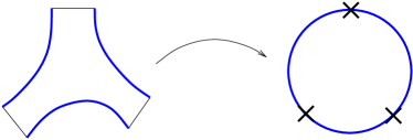
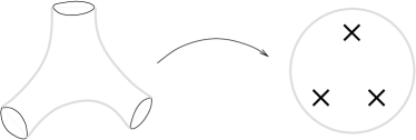
Figure 5.1: Open and closed strings conformally mapped to a disc and a sphere respectively. The background $B$-field affects only the open strings ending at the boundary of the disc and is not felt by the closed strings. Noncommutativity arises essentially since the open string vertex operators at the boundary of the disk cannot freely move past each other, while the closed string vertex operators in the bulk are not affected.

The propagator at boundary points compatible with the boundary conditions (5.3) is

$$\langle x^{i}(\tau)x^{j}(\tau^{\prime})\rangle=-\alpha^{\prime}{G^{ij}}\ln(\tau-\tau^{\prime})^{2}+\frac{i}{2}{\theta^{ij}}\varepsilon(\tau-\tau^{\prime}),$$ (5.4)

where $\varepsilon(\tau-\tau^{\prime})$ is the step function and

$$\frac{1}{g+2\pi\alpha^{\prime}B}=\frac{{\theta}}{2\pi\alpha^{\prime}}+\frac{1}{G(+2\pi\alpha^{\prime}\Phi)}.$$ (5.5)

(The term $2\pi\alpha^{\prime}\Phi$ is relevant in the so-called intermediate picture.) The correlation functions on the boundary of the disc in the decoupling limit ($g\rightarrow 0$, $\alpha^{\prime}\rightarrow 0$; $\theta=1/B$) for constant $B$ are

$$\left\langle f_{1}(x(\tau_{1}))\cdot\ldots\cdot f_{n}(x(\tau_{n}))\right\rangle_{B}=\int dx\,f_{1}\star\ldots\star f_{n},\quad(\tau_{1}<\ldots<\tau_{n})$$ (5.6)

with the Weyl-Moyal star product

$$(f\star g)(x)=\left.e^{\frac{i\hbar}{2}\theta^{i\!j}\partial_{i}\partial_{j}^{\prime}}f(x)g(x^{\prime})\right|_{x^{\prime}\rightarrow x},$$ (5.7)

which is the deformation quantization of the constant Poisson structure $\theta$. More generally a star product is an associative, $[[\hbar]]$-bilinear product

$$f\star g=fg+\sum_{n=1}^{\infty}(i\hbar)^{n}\underbrace{B_{n}(f,g)}_{\mathrm{bilinear}},$$ (5.8)

which is the deformation of a Poisson structure $\theta$:

$$[f\,\stackrel{{\scriptstyle\star}}{{,}}\,g]=i\hbar\{f\,,\,g\}+{\cal O}(\hbar^{2}),\quad\{f\,,\,g\}=\theta^{i\!j}(x)\partial_{i}f\,\partial_{j}g.$$ (5.9)

We now perturb the constant $B$ field by adding a gauge potential $a_{i}(x)$: $B\rightarrow B+da$, $S_{B}\rightarrow S_{B}+S_{a}$, with

$$S_{a}=-i\int_{\partial D}d\tau a_{i}(x(\tau))\partial_{\tau}x^{i}(\tau).$$ (5.10)

Classically we have the naive gauge invariance

$$\delta a_{i}=\partial_{i}\lambda,$$ (5.11)

but in the quantum theory this depends on the choice of regularization. For Pauli-Villars (5.11) remains a symmetry but if one expands $\exp S_{a}$ and employes a point-splitting regularization then the functional integral is invariant under noncommutative gauge transformations

$$\hat{\delta}\hat{A}_{i}=\partial_{i}\hat{\lambda}+i\hat{\lambda}\star\hat{A}_{i}-i\hat{A}_{i}\star\hat{\lambda}.$$ (5.12)

Since a sensible quantum theory should be independent of the choice of regularization there should be field redefinitions $\hat{A}(a)$, $\hat{\lambda}(a,\lambda)$ (Seiberg-Witten map) that relate (5.11) and (5.12):

$$\hat{A}(a)+\hat{\delta}_{\hat{\lambda}}\hat{A}(a)=\hat{A}(a+\delta_{\lambda}a).$$ (5.13)

It is instructive to study the effect of the extra factor $\exp S_{a}$ in the correlation function (5.6) in more detail: It effectively shifts the coordinates

$$x^{i}\rightarrow x^{i}+\theta^{ij}\hat{A}_{j}=:{\cal D}x^{i}.$$ (5.14)

More generally, for a function $f$,

$$f\rightarrow f+f_{A}=:{\cal D}f.$$ (5.15)

The mapping ${\cal A}:\,f\mapsto f_{A}$ plays the role of a generalized gauge potential; it maps a function to a new function that depends on the gauge potential. The shifted coordinates and functions are covariant under noncommutative gauge transformations:

$$\hat{\delta}({\cal D}x^{i})=i[\hat{\lambda}\,\stackrel{{\scriptstyle\star}}{{,}}\,{\cal D}x^{i}],\qquad\hat{\delta}({\cal D}f)=i[\hat{\lambda}\,\stackrel{{\scriptstyle\star}}{{,}}\,{\cal D}f].$$ (5.16)

The first expression implies (5.12) (for $\theta$ constant and nondegenerate).

The covariant coordinates (5.14) are the background independent operators of [128, 150]; they and the covariant functions (5.15) can also be introduced abstractly in the general case of an arbitrary noncommutative space as we shall discuss in the next section.

5.1 Gauge theory on noncommutative spaces

5.1.1 Covariant functions, covariant coordinates

Take a more or less arbitrary noncommutative space, i.e. an associative unital algebra $\mathcal{A}_{x}$ of noncommuting variables with multiplication $\star$ and consider (matter) fields $\psi$ on this space. The fields can be taken to be elements of $\mathcal{A}_{x}$, or, more generally, a left module of it. The notion of a gauge transformation is introduced as usual

$$\psi\mapsto\Lambda\star\psi,$$ (5.17)

where $\Lambda$ is an invertible element of $\mathcal{A}_{x}$. In analogy to commutative geometry where a manifold can be described by the commutative space of functions over it, we shall refer to the elements of $\mathcal{A}_{x}$ also as functions. Later we shall focus on the case where the noncommutative multiplication is a star product; the elements of $\mathcal{A}_{x}$ are then in fact ordinary functions in the usual sense of the word. The left-multiplication of a field with a function $f\in\mathcal{A}_{x}$ does in general not result in a covariant object because of the noncommutativity of $\mathcal{A}_{x}$:

$$f\star\psi\mapsto f\star\Lambda\star\psi\neq\Lambda\star(f\star\psi).$$ (5.18)

(As in ordinary gauge theory the gauge transformation only acts on the fields, i.e. on the elements of the left-module of $\mathcal{A}_{x}$ and not on the elements of $\mathcal{A}_{x}$ itself.) To cure (5.18) we introduce covariant functions

$${\cal D}f=f+f_{A},$$ (5.19)

that transform under gauge transformations by conjugation

$${\cal D}f\mapsto\Lambda\star{\cal D}f\star\Lambda^{-1},$$ (5.20)

by adding ‘gauge potentials’ $f_{A}$ with appropriate transformation property

$$f_{A}\mapsto\Lambda\star[f\,\stackrel{{\scriptstyle\star}}{{,}}\,\Lambda^{-1}]+\Lambda\star f_{A}\star\Lambda^{-1}.$$ (5.21)

Further covariant objects can be constructed from covariant functions; the ‘2-tensor’

$$\mathcal{F}(f,g)=[{\cal D}f\,\stackrel{{\scriptstyle\star}}{{,}}\,{\cal D}g]-{\cal D}([f\,\stackrel{{\scriptstyle\star}}{{,}}\,g]),$$ (5.22)

for instance plays the role of covariant noncommutative field strength.

Canonical structure (constant $\mathbf{\theta}$) and noncommutative Yang-Mills

Before we continue let us illustrate all this in the particular simple case of an algebra $\mathcal{A}_{x}$ generated by ‘coordinates’ $x^{i}$ with canonical commutation relations

$$[x^{i}\,\stackrel{{\scriptstyle\star}}{{,}}\,x^{j}]=i\theta^{ij},\quad\theta^{ij}\;\in\;{\mathbb{C}}.$$ (5.23)

This algebra arises in the decoupling limit of open strings in the presence of a constant $B$-field. It can be viewed as the quantization of a Poisson structure with Poisson tensor $\theta^{ij}$ and the multiplication $\star$ is then the Weyl-Moyal star product

$$f\star g=fe^{\frac{i}{2}\theta^{ij}\stackrel{{\scriptstyle\leftarrow}}{{\partial_{i}}}\otimes\stackrel{{\scriptstyle\rightarrow}}{{\partial_{j}}}}g.$$ (5.24)

(This formula holds only in the present example, where $\theta^{ij}$ is constant and we shall also assume that it is non-degenerate. In the rest of this chapter we drop both restrictions.) Let us focus on the coordinate functions $x^{i}$. The corresponding covariant coordinates are

$${\cal D}x^{i}=x^{i}+x_{A}^{i}=x^{i}+\theta^{ij}\hat{A}_{j},$$ (5.25)

where we have used $\theta$ to lower the index on $\hat{A}_{j}$. Using (5.23), we see that the transformation (5.21) of the noncommutative gauge potential $\hat{A}_{j}$ is

$$\hat{A}_{j}\mapsto i\Lambda\star\partial_{j}(\Lambda^{-1})+\Lambda\star\hat{A}_{j}\star\Lambda^{-1},$$ (5.26)

or, infinitesimally

$$\delta\hat{A}_{j}=\partial_{j}\lambda+i[\lambda,\hat{A}_{j}]_{\star}.$$ (5.27)

The noncommutative field strength

$$\hat{F}_{kl}=\partial_{k}\hat{A}_{l}-\partial_{l}\hat{A}_{k}-i[\hat{A}_{k},\hat{A}_{l}]_{\star}$$ (5.28)

transforms covariantly

$$\hat{F}_{kl}\mapsto\Lambda\star\hat{F}_{kl}\star\Lambda^{-1}.$$ (5.29)

We have again used $\theta$ to lower indices to get (5.28) from the definition (5.22)

$$i\hat{F}_{kl}\theta^{ik}\theta^{jl}\equiv\mathcal{F}(x^{i},x^{j})=[x_{A}^{i},x^{j}]_{\star}+[x^{i},x_{A}^{j}]_{\star}+[x_{A}^{i},x_{A}^{j}]_{\star}.$$ (5.30)

Note, that we should in general be more careful when using $\theta$ to lower indices as in (5.25) or (5.30) because this may spoil the covariance when $\theta$ is not constant as it was in this particular example. Relations (5.26), (5.28) and (5.29) define what is usually called Noncommutative Yang-Mills theory (NCYM) in the narrow sense: ordinary Yang-Mills with all matrix products replaced by star products. This simple rule, however, only really works well for the Moyal-Weyl product, i.e. constant $\theta$. In the general case it is wise to stick with the manifestly covariant and coordinate-independent objects defined in (5.19) and (5.22). The fundamental objects are really the mappings (differential operators) ${\cal D}$ and $\mathcal{F}$ in these equations. The transformation of ${\cal A}={\cal D}-\mbox{\small id}:f\mapsto f_{A}$ under gauge transformations is exactly so that (5.19) transforms by conjugation. The mappings ${\cal A}\in\mathrm{Hom}(\mathcal{A}_{x},\mathcal{A}_{x})$ and $\mathcal{F}\in\mathrm{Hom}(\mathcal{A}_{x}\wedge\mathcal{A}_{x},\mathcal{A}_{x})$ play the role of generalized noncommutative gauge potential and noncommutative field strength. There are several reasons, why one needs ${\cal A}$ and ${\cal D}$ and not just $A^{i}\equiv{\cal A}(x^{i})$ (or $\hat{A}_{i}$, for $\theta$ constant): If we perform a general coordinate transformation $x^{i}\mapsto{x^{i}}^{\prime}(x^{j})$ and transform $A^{i}$ (or $\hat{A}_{i}$) naively as its index structure suggests, then we would obtain objects that are no longer covariant under noncommutative gauge transformations. The correct transformation, ${\cal A}(x^{i})\mapsto{\cal A}^{\prime}({x^{i}}^{\prime})$, is more complicated and will be discussed in section 5.2.2. Furthermore we may be interested in covariant versions of scalar fields $\phi(x)$. These are given by the corresponding covariant function ${\cal D}(\phi(x))$.

In the next section we will propose an abstract definition of the type of noncommutative gauge theory that is of present interest. Then we shall proceed to give an interpretation in the framework of deformation quantization and will construct a particular important class of these operators.

5.1.2 Cochains and projective modules

Finite projective modules take the place of fiber bundles in the noncommutative realm [147]. This is also the case here, as we shall explain below, but may not have been apparent since we have been working with component fields as is customary in the physics literature. We have argued in the previous section that ${\cal A}\in C^{1}$, $\mathcal{F}\in C^{2}$ with $C^{p}=\mathrm{Hom}(\mathcal{A}_{x}^{\wedge p},\mathcal{A}_{x})$, $C^{0}\equiv\mathcal{A}_{x}$. These $p$-cochains take the place of forms on a noncommutative space $\mathcal{A}_{x}$, which for now is still an arbitrary associative algebra over a field $k$ with multiplication $\star$. It is actually more convenient to start with the Hochschild complex of $\mathcal{A}_{x}$, $H^{p}(\mathcal{A}_{x},\mathcal{A}_{x})=\mathrm{Hom}_{k}(\mathcal{A}_{x}^{\otimes p},\mathcal{A}_{x})$, with values in $\mathcal{A}_{x}$ considered as a left module of $\mathcal{A}_{x}$. (The formulas for $C^{p}$ can then be obtained by antisymmetrization.) We have a coboundary operator $\mathbf{d}_{\star}:H^{p}\rightarrow H^{p+1}$, $\mathbf{d}_{\star}^{2}=0$, $\mathbf{d}_{\star}1=0$,

$$\mathbf{d}_{\star}\mathcal{C}=-[\mathcal{C}\,,\,\star\,]_{\mathrm{G}},$$ (5.31)

where $[\,,\,]_{\mathrm{G}}$ is the Gerstenhaber bracket (A.4),

$$(\mathbf{d}_{\star}\mathcal{C})(f_{1},\ldots,f_{p+1})\;=\;f_{1}\star\mathcal{C}(f_{2},\ldots,f_{p+1})-\mathcal{C}(f_{1}\star f_{2},f_{3},\ldots,f_{p+1})+{}$$ (5.32)

$${}+\mathcal{C}(f_{1},f_{2}\star f_{3},\ldots,f_{p+1})\mp\cdots+(-)^{p}\mathcal{C}(f_{1},f_{2},\ldots,f_{p}\star f_{p+1})$$

$${}+(-)^{p+1}\mathcal{C}(f_{1},\ldots,f_{p})\star f_{p+1},$$

and we have a cup product $\star:H^{p_{1}}\otimes H^{p_{2}}\rightarrow H^{p_{1}+p_{2}}$,

$$\left(\mathcal{C}_{1}\star\mathcal{C}_{2}\right)\left(f_{1},\ldots,f_{p_{1}+p_{2}}\right)=\mathcal{C}_{1}(f_{1},\ldots,f_{p_{1}})\star\mathcal{C}_{2}(f_{p_{1}+1},\ldots,f_{p_{1}+p_{2}}).$$ (5.33)

For a function $\lambda\in H^{0}\equiv\mathcal{A}_{x}$ the coboundary operator is defined as

$$(\mathbf{d}_{\star}\lambda)(f)=f\star\lambda-\lambda\star f$$ (5.34)

and the cup product reduces to the multiplication $\star$ of $\mathcal{A}_{x}$ in the obvious way. For this reason and since there seems to be little chance of confusion we have used the same symbol $\star$ for the cup product and the multiplication. Let us apply the Hochschild formalism to the gauge transformation dependent map ${\cal D}\in H^{1}$ that we introduced in the definition of covariant functions (5.19) in the previous section. In view of the way that $A^{i}\equiv\theta^{ij}\hat{A}_{j}$ appeared in the definition of covariant coordinates (5.25) we define an abstract noncommutative gauge potential ${\cal A}\in H^{1}$

$${\cal A}\equiv{\cal D}-\mbox{\small id}.$$ (5.35)

Applying ${\cal A}$ to coordinate functions in the setting of (5.25) we indeed recover $A^{i}$:

$${\cal A}(x^{i})={\cal D}(x^{i})-x^{i}=A^{i}.$$

Let us compute the behavior of ${\cal A}$ under a gauge transformation. Using (5.20) and the definitions of $\mathbf{d}_{\star}$ and the cup product we find

$${\cal A}\mapsto\Lambda\star\mathbf{d}_{\star}\Lambda^{-1}+\Lambda\star{\cal A}\star\Lambda^{-1},$$ (5.36)

which gives (5.21) when evaluated on a function. The corresponding infinitesimal version is

$$\delta{\cal A}=i(-\mathbf{d}_{\star}\lambda+\lambda\star{\cal A}-{\cal A}\star\lambda).$$ (5.37)

Next we introduce the “Hochschild” field strength $\mathcal{F}_{H}\in H^{2}$

$$\mathcal{F}_{H}\equiv\mathbf{d}_{\star}{\cal A}+{\cal A}\star{\cal A}$$ (5.38)

and compute

$$\mathcal{F}_{H}(f,g)={\cal D}f\star{\cal D}g-{\cal D}(f\star g)$$ (5.39)

and find the Bianchi identity

$$\mathbf{d}_{\star}\mathcal{F}_{H}+{\cal A}\star\mathcal{F}_{H}-\mathcal{F}_{H}\star{\cal A}=0.$$ (5.40)

Evaluated on three functions $f$, $g$, $h$ the latter reads

$${\cal D}((f\star g)\star h)-{\cal D}(f\star(g\star h))+({\cal D}f\star{\cal D}g)\star{\cal D}h-{\cal D}f\star({\cal D}g\star{\cal D}h),$$ (5.41)

which is zero by associativity of $\mathcal{A}_{x}$. $\mathcal{F}_{H}$ transforms covariantly under gauge transformations

$$\mathcal{F}_{H}\mapsto\Lambda\star\mathcal{F}_{H}\star\Lambda^{-1};$$ (5.42)

infinitesimally

$$\delta\mathcal{F}_{H}=i(\lambda\star\mathcal{F}_{H}-\mathcal{F}_{H}\star\lambda).$$ (5.43)

When we compare (5.22) and (5.39), we see (as expected) that our noncommutative field strength $\mathcal{F}$ of the previous section is an antisymmetric version of $\mathcal{F}_{H}$. We can obtain $\mathcal{F}$ directly by taking the antisymmetrized version of Hochschild, where one considers $\mathcal{A}_{x}$ as a Lie algebra with bracket $[a\,\stackrel{{\scriptstyle\star}}{{,}}\,b]=a\star b-b\star a$; this is the Chevalley cohomology of $\mathcal{A}_{x}$ with values in $\mathcal{A}_{x}$: $C^{p}=\mathrm{Hom}_{k}(\mathcal{A}_{x}^{\wedge p},\mathcal{A}_{x})$. We find the relevant formulas in this setting by replacing $H^{p}$ with $C^{p}$ (whose elements are antisymmetric), and by using corresponding antisymmetrized formulas for the coboundary operator $\mathbf{d}_{\star}$ and the cup product which we then denote by $\wedge$. The action of $\mbox{Lie}\mathcal{A}_{x}$ on the module $\mathcal{A}_{x}$ is given by $\star$-multiplication as before. We now see that equation (5.22),

$$\mathcal{F}(f,g)=[{\cal D}f\,\stackrel{{\scriptstyle\star}}{{,}}\,{\cal D}g]-{\cal D}([f\,\stackrel{{\scriptstyle\star}}{{,}}\,g]),$$ (5.44)

can be written

$$\mathcal{F}\equiv\mathbf{d}_{\star}{\cal A}+{\cal A}\wedge{\cal A}.$$ (5.45)

The remaining equations also do not change in form (as compared to the Hochschild case): (5.45) implies

$$\mathbf{d}_{\star}\mathcal{F}+{\cal A}\wedge\mathcal{F}-\mathcal{F}\wedge{\cal A}=0$$ (5.46)

and the behavior under (infinitesimal )gauge transformations is

$$\delta{\cal A} = i(-\mathbf{d}_{\star}\lambda+\lambda\wedge{\cal A}-{\cal A}\wedge\lambda),$$ (5.47)

$$\delta\mathcal{F} = i\left(\lambda\wedge\mathcal{F}-\mathcal{F}\wedge\lambda\right).$$ (5.48)

Equations (5.45), (5.46), (5.47) and (5.48) are reminiscent of the corresponding equations of ordinary (nonabelian) gauge theory. The correspondence is given by the following dictionary: One-forms become linear operators on $\mathcal{A}_{x}$ which take one function as argument and yield a new function, two-forms become bilinear operators on $\mathcal{A}_{x}$ which take two functions as arguments and return one new function, and the Lie bracket is replaced by the antisymmetrized cup product $\wedge$. As in ordinary gauge theory, it may not be possible to use one globally defined gauge potential ${\cal A}$; we may need to introduce several ${\cal D}$ and corresponding gauge potentials ${\cal A}$ for functions defined on different “patches”. We shall come back to this later.

Remark: One reason for going through the slightly more general Hochschild construction first is that the symmetric part of $\mathcal{F}_{H}$ may also contain interesting information as we will see in section 5.2.4. For invertible ${\cal D}$ there is still another interesting object:

$$\widetilde{\mathcal{F}}\equiv{\cal D}^{-1}\circ\mathcal{F}$$ (5.49)

measures noncommutativity:

$$\widetilde{\mathcal{F}}(f,g)=[f\stackrel{{\scriptstyle\star^{\prime}}}{{,}}g]-[f\stackrel{{\scriptstyle\star}}{{,}}g],$$ (5.50)

where the (associative) product $\star^{\prime}$ is defined by $f\star^{\prime}g={\cal D}^{-1}\Big{(}{\cal D}f\star{\cal D}g\Big{)}$. This “field strength” satisfies the Cartan-Maurer equation

$$\mathbf{d}_{\star}\widetilde{\mathcal{F}}=[\widetilde{\mathcal{F}}\,,\,\widetilde{\mathcal{F}}]_{\mathrm{G}}.$$ (5.51)

Projective modules

We shall now discuss how our formulae fit into the framework of finite projective modules: The calculus of $p$-cochains in $C^{p}$ with the coboundary operator $\mathbf{d}_{\star}$ uses only the algebraic structure of $\mathcal{A}_{x}$; it is related to the standard universal calculus and one can obtain other calculi by projection. Consider a (finite) projective right $\mathcal{A}_{x}$-module ${\cal E}$. We introduce a connection on ${\cal E}$ as a linear map $\nabla:{\cal E}\otimes_{\mathcal{A}_{x}}\!C^{p}\rightarrow{\cal E}\otimes_{\mathcal{A}_{x}}C^{p+1}$ for $p\in\mathbb{N}_{0}$ which satisfies the Leibniz rule

$$\nabla(\eta\psi)=(\tilde{\nabla}\eta)\psi+(-)^{p}\eta\,\mathbf{\tilde{d}}_{\star}\psi$$

for all $\eta\in{\cal E}\otimes_{\mathcal{A}_{x}}\!C^{p}$, $\psi\in C^{r}$, and where $\tilde{\nabla}\eta=\nabla\eta-(-)^{p}\eta\,\mathbf{\tilde{d}}_{\star}1$,

$$\mathbf{\tilde{d}}_{\star}(a\wedge\psi)=(\mathbf{d}_{\star}a)\wedge\psi+(-)^{q}a\wedge(\mathbf{\tilde{d}}_{\star}\psi)$$ (5.52)

for all $a\in C^{q}$, and $\mathbf{\tilde{d}}_{\star}1$ is the identity operator on $\mathcal{A}_{x}$. (The transformation of matter fields $\hat{\delta}\psi=i\hat{\lambda}\star\psi$ leads to a slight complication here; for fields that transform in the adjoint (by star-commutator) we would only need $\tilde{\nabla}$, $\mathbf{d}_{\star}$ and not $\nabla$ and $\mathbf{\tilde{d}}_{\star}$.) Let $(\eta_{a})$ be a generating family for ${\cal E}$; any $\xi\in{\cal E}$ can then be written as $\xi=\sum\eta_{a}\psi^{a}$ with $\psi^{a}\in\mathcal{A}_{x}$ (with only a finite number of terms different from zero). For a free module the $\psi^{a}$ are unique, but we shall not assume that. Let the generalized gauge potential be defined by the action of $\tilde{\nabla}$ on the elements of the generating family: $\tilde{\nabla}\eta_{a}=\eta_{b}{\cal A}^{b}_{a}$. In the following we shall suppress indices and simply write $\xi=\eta.\psi$, $\tilde{\nabla}\eta=\eta.{\cal A}$ etc. We compute

$$\nabla\xi=\nabla(\eta.\psi)=\eta.({\cal A}\wedge\psi+\mathbf{\tilde{d}}_{\star}\psi)=\eta.({\cal D}\wedge\psi).$$ (5.53)

Evaluated on a function $f\in\mathcal{A}_{x}$ the component ${\cal D}\wedge\psi$ yields a covariant function times the matter field, $({\cal D}\wedge\psi)(f)=({\cal D}f)\star\psi$, so in this framework covariant functions are related to the covariant “derivative” $\mathbf{\tilde{d}}_{\star}+{\cal A}$:

$$[(\mathbf{\tilde{d}}_{\star}+{\cal A})\psi](f)=(f+{\cal A}(f))\star\psi.$$ (5.54)

The square of the connection gives

$$\nabla^{2}\xi=\eta.({\cal A}\wedge{\cal A}+\mathbf{d}_{\star}{\cal A}).\psi=\eta.\mathcal{F}.\psi$$ (5.55)

with the field strength

$$\mathcal{F}=\mathbf{d}_{\star}{\cal A}+{\cal A}\wedge{\cal A}.$$ (5.56)

5.2 Ordinary versus noncommutative gauge theory

We are particularly interested in the case where the algebra of our noncommutative space $\mathcal{A}_{x}$ is given by a star product (via a quantization map). A star product on a smooth $C^{\infty}$-Manifold ${\cal M}$ is an associative ${\mathbb{C}}[[\hbar]]$-bilinear product

$$f\star g=fg+\sum_{n=1}^{\infty}\left(\frac{i\hbar}{2}\right)^{n}B_{n}(f,g),\quad f,g\in C^{\infty}({\cal M}),$$ (5.57)

where $B_{n}$ are bilinear operators and $\hbar$ is the formal deformation parameter; it is a deformation quantization of the Poisson structure

$$\{f,g\}\equiv\theta^{ij}(x)\partial_{i}f\,\partial_{j}g=B_{1}(f,g)-B_{1}(g,f).$$ (5.58)

Equivalent star products $\tilde{\star}$ can be constructed with the help of invertible operators $D$

$$D(f\,\tilde{\star}\,g)=Df\star Dg,\qquad Df\equiv f+\sum_{n=1}^{\infty}\hbar^{n}D_{n}(f),$$ (5.59)

where $D_{n}$ are linear operators. This operation clearly does not spoil associativity. There are also inner automorphisms for each invertible element $\Lambda$ and their infinitesimal version, inner derivations,

$$f\mapsto\Lambda\star f\star\Lambda^{-1},\qquad\delta f=[i\lambda\,\stackrel{{\scriptstyle\star}}{{,}}\,f];$$ (5.60)

these operations do not change the star product.

The striking similarity between equations (5.19), (5.20) and equations (5.59), (5.60) suggests the following interpretation of noncommutative gauge theory in the star product formalism: The covariance maps ${\cal D}=\mbox{\small id}+{\cal A}$ are gauge equivalence maps $D$ for the underlying star product, combined with a change of coordinates $\rho^{*}$

$${\cal D}=D\circ\rho^{*},\qquad{\cal D}(f\star^{\prime}g)={\cal D}f\star{\cal D}g;$$ (5.61)

gauge transformations are inner automorphisms of the star products.

Motivation from string theory

A Poisson tensor $\theta$ enters the discussion of Seiberg and Witten [128] via a background $B$-field in the open string picture. In this setting

$$\theta^{ij}=2\pi\alpha^{\prime}\left(\frac{1}{g+2\pi\alpha^{\prime}B}\right)^{ij}_{A}$$ (5.62)

appears in the propagator at boundary points of the string world sheet. ($g$ is the closed string metric and $A$ denotes the antisymmetric part of a matrix.) The 2-form $\omega\equiv\frac{1}{2}B_{ij}dx^{i}\wedge dx^{j}$ is a symplectic form, provided $B$ is nondegenerate and $d\omega=0$, which is e.g. obviously the case if $B$ is constant (but we shall not require it to be constant.) In the zero slope limit (or in the intermediate picture with $\Phi=-B$ [128], see section 5.2.3)

$$\theta^{ij}=(B^{-1})^{ij}$$ (5.63)

defines then a Poisson structure. It has been discussed by several authors how the Moyal-Weyl star product enters the picture as a quantization of this Poisson structure in the constant case [122, 123, 128]. A direct approach that is most suitable for our purposes and that also works for non-constant $\theta$ is given by Cattaneo and Felder [137] in their QFT realization of Kontsevich’s star product.

In the introduction we have discussed what happens if we add fluctuations $f$ (with $df=0$, i.e. locally $f=da$) to the background $B$ field: The action is then naively invariant under ordinary gauge transformations $\delta a=d\lambda$, but the invariance of the quantum theory depends on the choice of regularization. A point splitting prescription [128, 129] leads in fact to a noncommutative gauge invariance. Since in a consistent quantum theory the choice of regularization should not matter, Seiberg and Witten argued that there should exist maps that relate ordinary and noncommutative gauge theory such that (5.1) holds. A more abstract argument that leads to the same conclusion, but gives the Seiberg-Witten maps more directly and also works for non-constant $\theta$ can be based on a quantum version of Moser’s lemma [130, 131]. Here is briefly the idea, in the next section we will review the details: The addition of $f=da$ to $B$ defines a new Poisson structure

$$\theta=\frac{1}{B}\quad\rightarrow\quad\theta^{\prime}=\frac{1}{B+f}$$ (5.64)

which, according to Moser’s lemma, is related to the original one by a change of coordinates given by a flow $\rho^{*}_{a}$ that depends on the gauge potential $a$. After quantization $\theta$ and $\theta^{\prime}$ give rise to equivalent star products $\star$ and $\star^{\prime}$. The equivalence map $D_{a}$, the full quantum flow ${\cal D}_{a}=D_{a}\circ\rho^{*}_{a}$ and the noncommutative gauge potential

$${\cal A}_{a}={\cal D}_{a}-\mbox{\small id}$$ (5.65)

are also functions of $a$. An additional infinitesimal gauge transformation

$$\delta a=d\lambda$$ (5.66)

does not change the Poisson structure (since $\delta f=0$), but it still induces an infinitesimal canonical transformation. After quantization that transformation becomes an inner derivation of the star product $\star$ and thus a noncommutative gauge transformation $\delta_{\hat{\lambda}}$ with $\hat{\lambda}=\hat{\lambda}(\lambda,a)$, such that

$${\cal A}_{a+d\lambda}={\cal A}_{a}+\delta_{\hat{\lambda}}{\cal A}_{a}.$$ (5.67)

5.2.1 Seiberg-Witten map and Kontsevich formality

Consider an abelian gauge theory on a manifold that also carries a Poisson structure $\theta$. The gauge potential, field strength and infinitesimal gauge transformations are

$$a=a_{i}dx^{i},\qquad f=\frac{1}{2}f_{ij}\,dx^{i}\wedge dx^{j}=da,\qquad f_{ij}=\partial_{i}a_{j}-\partial_{j}a_{i},\qquad\delta_{\lambda}a=d\lambda.$$ (5.68)

We will first construct a semiclassical version of the Seiberg-Witten map, where all star commutators are replaced by Poisson brackets. The construction is essentially a formal generalization of Moser’s lemma to Poisson manifolds.

Semi-classical construction

Let us consider the nilpotent coboundary operator of the Poisson cohomology (see [164]) – the semiclassical limit of (5.31) –

$$\mathbf{d}_{\theta}=-[\,\cdot\,\,,\,\theta]_{\mathrm{S}},$$ (5.69)

where $[\,,\,]_{\mathrm{S}}$ is the Schouten-Nijenhuis bracket (A.1) and $\theta=\frac{1}{2}\theta^{ij}\partial_{i}\wedge\partial_{j}$ is the Poisson bivector. Acting with $\mathbf{d}_{\theta}$ on a function $f$ gives the Hamiltonian vector field corresponding to $f$

$$\mathbf{d}_{\theta}f=\{\,\cdot\,,f\}=\theta^{ij}(\partial_{j}f)\partial_{i}.$$ (5.70)

It is natural to introduce a vector field

$$\mathbf{a}_{\theta}=a_{i}\mathbf{d}_{\theta}x^{i}=\theta^{ji}a_{i}\partial_{j}$$ (5.71)

corresponding to the abelian gauge potential $a$ and a bivector field

$$\mathbf{f}_{\theta}=\mathbf{d}_{\theta}\mathbf{a}_{\theta}=-\frac{1}{2}\theta^{ik}f_{kl}\theta^{lj}\,\partial_{i}\wedge\partial_{j}$$ (5.72)

corresponding to the abelian field strength $f=da$. We have $\mathbf{d}_{\theta}\mathbf{f}_{\theta}=0$, due to $\mathbf{d}_{\theta}^{2}\propto[\theta\,,\,\theta]_{\mathrm{S}}=0$ (Jacobi identity).

We are now ready to perturb the Poisson structure $\theta$ by introducing a one-parameter deformation $\theta_{t}$ with $t\in[0,1]$:

$$\partial_{t}\theta_{t}=\mathbf{f}_{\theta_{t}}$$ (5.73)

with initial condition $\theta_{0}=\theta$. In local coordinates:

$$\partial_{t}\theta_{t}^{ij}=-(\theta_{t}f\theta_{t})^{ij},\qquad\theta_{0}^{ij}=\theta^{ij},$$ (5.74)

with formal solution given by the geometric series

$$\theta_{t}=\theta-t\theta f\theta+t^{2}\theta f\theta f\theta-t^{3}\theta f\theta f\theta f\theta\pm\cdots=\theta\frac{1}{1+tf\theta},$$ (5.75)

if $f$ is not explicitly $\theta$-dependent. (The differential equations (5.73), (5.74) and the rest of the construction do make sense even if $f$ or $a$ are $\theta$-dependent). $\theta_{t}$ is a Poisson tensor for all $t$ because $[\theta_{t}\,,\,\theta_{t}]_{\mathrm{S}}=0$ at $t=0$ and

$$\partial_{t}[\theta_{t}\,,\,\theta_{t}]_{\mathrm{S}}=-2\mathbf{d}_{\theta_{t}}\mathbf{f}_{\theta_{t}}\propto[\theta_{t}\,,\,\theta_{t}]_{\mathrm{S}}.$$

The evolution (5.73) of $\theta_{t}$ is generated by the vector field $\mathbf{a}_{\theta}$:

$$\partial_{t}\theta_{t}=\mathbf{d}_{\theta_{t}}\mathbf{a}_{\theta_{t}}=-[\mathbf{a}_{\theta_{t}}\,,\,\theta_{t}]_{\mathrm{S}}.$$ (5.76)

This Lie derivative can be integrated to a flow (see appendix A.2)

$$\rho^{*}_{a}=\left.\exp(\mathbf{a}_{\theta_{t}}+\partial_{t})\exp(-\partial_{t})\right|_{t=0}$$ (5.77)

that relates the Poisson structures $\theta^{\prime}=\theta_{1}$ and $\theta=\theta_{0}$. In analogy to (5.35) we define a semi-classical (semi-noncommutative) generalized gauge potential

$$A_{a}=\rho^{*}_{a}-\mbox{\small id}.$$ (5.78)

Under an infinitesimal gauge transformation $a\mapsto a+d\lambda$ the vector field (5.71) changes by a Hamiltonian vector field $\mathbf{d}_{\theta}\lambda=\theta^{ij}(\partial_{j}\lambda)\partial_{i}$:

$$\mathbf{a}_{\theta}\mapsto\mathbf{a}_{\theta}+\mathbf{d}_{\theta}\lambda.$$ (5.79)

Let us compute the effect of this gauge transformation on the flow (5.77). After some computation (see appendix A.3) we find (infinitesimally: to first order in $\lambda$)

$$\rho^{*}_{a+d\lambda}=(\mbox{\small id}+\mathbf{d}_{\theta}\tilde{\lambda})\circ\rho^{*}_{a},\quad\mbox{i.e.,}\quad\rho^{*}_{a+d\lambda}(f)=\rho^{*}_{a}(f)+\{\rho^{*}_{a}(f),\tilde{\lambda}\}$$ (5.80)

and

$$A_{a+d\lambda}=A_{a}+\,\mathbf{d}_{\theta}\tilde{\lambda}+\{A_{a},\tilde{\lambda}\},$$ (5.81)

with

$$\tilde{\lambda}(\lambda,a)=\sum_{n=0}^{\infty}\left.\frac{(\mathbf{a}_{\theta_{t}}+\partial_{t})^{n}(\lambda)}{(n+1)!}\right|_{t=0}.$$ (5.82)

Equations (5.82) and (5.78) with (5.77) are explicit semi-classical versions of the Seiberg-Witten map. The semi-classical (semi-noncommutative) generalized field strength evaluated on two functions (e.g. coordinates) $f$, $g$ is

$$F_{a}(f,g)=\{\rho^{*}f\,,\,\rho^{*}g\}-\rho^{*}\{f\,,\,g\}=\rho^{*}\left(\{f\,,\,g\}^{\prime}-\{f\,,\,g\}\right).$$ (5.83)

Abstractly as 2-cochain:

$$F_{a}=\rho^{*}\circ\frac{1}{2}(\theta^{\prime}-\theta)^{ik}\partial_{i}\wedge\partial_{k}=\rho^{*}\circ\frac{1}{2}(f^{\prime})_{jl}\theta^{ij}\theta^{kl}\partial_{i}\wedge\partial_{k}$$ (5.84)

with $\theta^{\prime}f=\theta f^{\prime}$, or

$$f^{\prime}=\frac{1}{1+f\theta}f,$$ (5.85)

which we recognize as the noncommutative field strength (with lower indices) for constant $f$, $\theta$ [128]. The general result for non-constant $f$, $\theta$ is thus simply obtained by the application of the covariantizing map $\rho^{*}$ (after raising indices with $\theta$’s).

The Seiberg-Witten map in the semiclassical regime for constant $\theta$ has previously been discussed in [151, 153], where it was understood as a coordinate redefinition that eliminates fluctuations around a constant background.

We will now use Kontsevich’s formality theorem to quantize everything. The goal is to obtain (5.1) in the form (5.67) of which (5.81) is the semi-classical limit.

Kontsevich formality map

Kontsevich’s formality map is a collection of skew-symmetric multilinear maps $U_{n}$ for $n=0\ldots\infty$ that map tensor products of $n$ polyvector fields to differential operators. More precisely $U_{n}$ maps the tensor product of $n$ $k_{i}$-vector fields to an $m$-differential operator, where $m$ is determined by the matching condition

$$m=2-2n+\sum_{i=1}^{n}k_{i}.$$ (5.86)

$U_{1}$ in particular is the natural map from a $k$-vector field to a $k$-differential operator

$$U_{1}(\xi_{1}\wedge\ldots\wedge\xi_{k})(f_{1},\ldots,f_{k})=\frac{1}{k!}\sum_{\sigma\in\Sigma_{k}}\mathrm{sgn}(\sigma)\prod_{i=1}^{k}\xi_{\sigma_{i}}(f_{i}),$$ (5.87)

and $U_{0}$ is defined to be the ordinary multiplication of functions:

$$U_{0}(f,g)=fg.$$ (5.88)

The $U_{n}$, $n\geq 1$, satisfy the formality condition [132]

$$d_{\mu}U_{n}(\alpha_{1},\ldots,\alpha_{n})+\frac{1}{2}\sum_{{}^{I\sqcup J=(1,\ldots,n)}_{I,J\neq\emptyset}}\pm[U_{|I|}(\alpha_{I})\,,\,U_{|J|}(\alpha_{J})]_{\mathrm{G}}$$ (5.89)

$$=\sum_{i<j}\pm U_{n-1}\left([\alpha_{i}\,,\,\alpha_{j}]_{\mathrm{S}},\alpha_{1},\ldots,\widehat{\alpha}_{i},\ldots,\widehat{\alpha}_{j},\ldots,\alpha_{n}\right),$$

where $d_{\mu}{\cal C}\equiv-[{\cal C}\,,\,\mu]_{\mathrm{G}}$, with the commutative multiplication $\mu(f,g)=f\cdot g$ of functions; the hat marks an omitted vector field. See [132, 137] for explicit constructions and more details and [155, 132] for the definition of the signs in this equation. In the following we collect the three special cases that we actually use in this chapter.

Consider the formal series (see also [156])

$$\Phi(\alpha)=\sum_{n=0}^{\infty}\frac{(i\hbar)^{n}}{n!}U_{n+1}(\alpha,\theta,\ldots,\theta).$$ (5.90)

According to the matching condition (5.86), $U_{n+1}(\alpha,\theta,\ldots,\theta)$ is a tridifferential operator for every $n$ if $\alpha$ is a trivector field, it is a bidifferential operator if $\alpha$ is a bivector field, it is a differential operator if $\alpha$ is a vector field and it is a function if $\alpha$ is a function; in all cases $\theta$ is assumed to be a bidifferential operator.

Star products from Poisson tensors

A Poisson bivector $\theta$ gives rise to a star product via the formality map: According to the matching condition (5.86), $U_{n}(\theta,\ldots,\theta)$ is a bidifferential operator for every $n$ if $\theta$ is a bivector field. This can be used to define a product

$$f\star g=\sum_{n=0}^{\infty}\frac{\left(i\hbar\right)^{n}}{n!}U_{n}(\theta,\ldots,\theta)(f,g)=fg+\frac{i\hbar}{2}\,\theta^{ij}\partial_{i}f\,\partial_{j}g+\cdots\;.$$ (5.91)

The formality condition implies

$$\mathbf{d}_{\star}\star=i\hbar\Phi(\mathbf{d}_{\theta}\theta),$$ (5.92)

or, $[\star\,,\,\star]_{\mathrm{G}}=i\hbar\Phi([\theta\,,\,\theta]_{\mathrm{S}})$, i.e., associativity of $\star$, if $\theta$ is Poisson. (If $\theta$ is not Poisson, i.e., has non-vanishing Schouten-Nijenhuis bracket $[\theta\,,\,\theta]_{\mathrm{S}}$, then the product $\star$ is not associative, but the non-associativity is nevertheless under control via the formality condition by (5.92).)

Differential operators from vector fields

We can define a linear differential operator

$$\Phi(\xi)=\xi+\frac{(i\hbar)^{2}}{2}U_{3}(\xi,\theta,\theta)+\cdots$$ (5.93)

for every vector field $\xi$. For $\theta$ Poisson the formality condition gives

$$\mathbf{d}_{\star}\Phi(\xi)=i\hbar\Phi(\mathbf{d}_{\theta}\xi)=i\hbar\,\mathbf{d}_{\theta}\xi+\cdots\;.$$ (5.94)

Vector fields $\xi$ that preserve the Poisson bracket, $\mathbf{d}_{\theta}\xi=-[\theta\,,\,\xi]_{\mathrm{S}}=0$, give rise to derivations of the star product (5.91): From (5.94) and the definition (A.7), (5.32) of $\mathbf{d}_{\star}$

$$0=[\mathbf{d}_{\star}\Phi(\xi)](f,g)=-[\Phi(\xi)](f\star g)+f\star[\Phi(\xi)](g)+[\Phi(\xi)](f)\star g.$$ (5.95)

Inner derivations from Hamiltonian vector fields

Hamiltonian vector fields $\mathbf{d}_{\theta}f$ give rise to inner derivations of the star product (5.91): We can define a new function

$$\hat{f}\equiv\Phi(f)=f+\frac{(i\hbar)^{2}}{2}U_{3}(f,\theta,\theta)+\cdots$$ (5.96)

for every function $f$. For $\theta$ Poisson the formality condition gives

$$\mathbf{d}_{\star}\hat{f}=i\hbar\Phi(\mathbf{d}_{\theta}f)$$ (5.97)

Evaluated on a function $g$, this reads

$$[\Phi(\mathbf{d}_{\theta}f)](g)=\frac{1}{i\hbar}[g\,\stackrel{{\scriptstyle\star}}{{,}}\,\hat{f}].$$ (5.98)

The Hamiltonian vector field $\mathbf{d}_{\theta}f$ is thus mapped to the inner derivation $\frac{i}{\hbar}[\hat{f}\,\stackrel{{\scriptstyle\star}}{{,}}\,\,\cdot\,]$.

Quantum construction

The construction mirrors the semiclassical one, the exact correspondence is given by the formality maps $U_{n}$ that are skew-symmetric multilinear maps that take $n$ polyvector fields into a polydifferential operator. We start with the differential operator

$$\mathbf{a}_{\star}=\sum_{n=0}^{\infty}\frac{\left(i\hbar\right)^{n}}{n!}U_{n+1}(\mathbf{a}_{\theta},\theta,\ldots,\theta),$$ (5.99)

which is the image of the vector field $\mathbf{a}_{\theta}$ under the formality map (5.93); then we use the coboundary operator $\mathbf{d}_{\star}$ (5.31) to define a bidifferential operator

$$\mathbf{f}_{\star}=\mathbf{d}_{\star}\mathbf{a}_{\star}.$$ (5.100)

This is the image of $\mathbf{f}_{\theta}=\mathbf{d}_{\theta}\mathbf{a}_{\theta}$ under the formality map:

$$\mathbf{f}_{\star}=\sum_{n=0}^{\infty}\frac{(i\hbar)^{n+1}}{n!}U_{n+1}(\mathbf{f}_{\theta},\theta,\ldots,\theta).$$ (5.101)

A $t$-dependent Poisson structure (5.73) induces a $t$-dependent star product via (5.91)

$$g\star_{t}h=\sum_{n=0}^{\infty}\frac{(i\hbar)^{n}}{n!}U_{n}(\theta_{t},\ldots,\theta_{t})(g,h).$$ (5.102)

The $t$-derivative of this equation is

$$\partial_{t}(g\star_{t}h)=\sum_{n=0}^{\infty}\frac{(i\hbar)^{n+1}}{n!}U_{n+1}(\mathbf{f}_{\theta_{t}},\theta_{t},\ldots,\theta_{t})(g,h),$$ (5.103)

where we have used (5.73) and the skew-symmetry and multi-linearity of $U_{n}$. Comparing with (5.101) we find

$$\partial_{t}(g\star_{t}h)=\mathbf{f}_{\star_{t}}(g,h),$$ (5.104)

or, shorter, as an operator equation: $\partial_{t}(\star_{t})=\mathbf{f}_{\star_{t}}$. But $\mathbf{f}_{\star_{t}}=\mathbf{d}_{\star_{t}}\mathbf{a}_{\star_{t}}=-[\mathbf{a}_{\star_{t}}\,,\,\star_{t}]_{\mathrm{G}}$, so the $t$-evolution is generated by the differential operator $\mathbf{a}_{\star_{t}}$ and can be integrated to a flow (see appendix A.2)

$${\cal D}_{a}=\left.\exp(\mathbf{a}_{\star_{t}}+\partial_{t})\exp(-\partial_{t})\right|_{t=0},$$ (5.105)

that relates the star products $\star^{\prime}=\star_{1}$ and $\star=\star_{0}$, and that defines the generalized noncommutative gauge potential

$${\cal A}_{a}={\cal D}_{a}-\mbox{\small id}.$$ (5.106)

The transformation of $\mathbf{a}_{\star}$ under an infinitesimal gauge transformation $a\mapsto a+d\lambda$ can be computed from (5.79) with the help of (5.97), see (5.34):

$$\mathbf{a}_{\star}\mapsto\mathbf{a}_{\star}+\frac{1}{i\hbar}\mathbf{d}_{\star}\hat{\lambda}.$$ (5.107)

The effect of this transformation on the quantum flow and on the noncommutative gauge potential are (see appendix A.3)

$${\cal D}_{a+d\lambda}=(\mbox{\small id}+\frac{1}{i\hbar}\mathbf{d}_{\star}\hat{\Lambda})\circ{\cal D}_{a},\quad\mbox{i.e.,}\quad{\cal D}_{a+d\lambda}(f)={\cal D}_{a}f+\frac{i}{\hbar}[\hat{\Lambda}\,\stackrel{{\scriptstyle\star}}{{,}}\,{\cal D}_{a}f]$$ (5.108)

$${\cal A}_{a+d\lambda}={\cal A}_{a}+\frac{1}{i\hbar}\left(\mathbf{d}_{\star}\hat{\Lambda}-\hat{\Lambda}\star{\cal A}+{\cal A}\star\hat{\Lambda}\right).$$ (5.109)

with

$$\hat{\Lambda}(\lambda,a)=\sum_{n=0}^{\infty}\left.\frac{(\mathbf{a}_{\star_{t}}+\partial_{t})^{n}(\hat{\lambda})}{(n+1)!}\right|_{t=0}.$$ (5.110)

Equations (5.106) with (5.105) and (5.110) are explicit versions of the abelian Seiberg-Witten map to all orders in $\hbar$. They are unique up to (noncommutative) gauge transformations. Perhaps more importantly this construction provides us with an explicit version of the “covariantizer” ${\cal D}_{a}$ (the equivalence map that sends coordinates and functions to their covariant analogs) in terms of a finite number of (classical) fields $a_{i}$. The noncommutative gauge parameter (5.110) also satisfies the consistency condition

$$\delta_{\alpha}\hat{\Lambda}(\beta,a)-\delta_{\beta}\hat{\Lambda}(\alpha,a)=\frac{i}{\hbar}[\hat{\Lambda}(\alpha,a)\,\stackrel{{\scriptstyle\star}}{{,}}\,\hat{\Lambda}(\beta,a)],$$ (5.111)

with $\delta_{\alpha}(a_{i})=\partial_{i}\alpha$, $\delta_{\alpha}(\beta)=0$, that follows from computing the commutator of abelian gauge transformations on a covariant field [9].

The generalized noncommutative field strength evaluated on two functions (or coordinates) $f$, $g$ is

$$\mathcal{F}_{a}(f,g)={\cal D}_{a}\left([f\stackrel{{\scriptstyle\star^{\prime}}}{{,}}g]-[f\,\stackrel{{\scriptstyle\star}}{{,}}\,g]\right).$$ (5.112)

Up to order $\theta^{2}$ the series for ${\cal A}_{a}$ and $\Lambda$ agree with the semiclassical results. In components:

$${\cal A}_{a}(x^{i})=\theta^{ij}a_{j}+\frac{1}{2}\theta^{kl}a_{l}(\partial_{k}(\theta^{ij}a_{j})-\theta^{ij}f_{jk})+\ldots,$$ (5.113)

$$\hat{\Lambda}=\lambda+\frac{1}{2}\theta^{ij}a_{j}\partial_{i}\lambda+\frac{1}{6}\theta^{kl}a_{l}(\partial_{k}(\theta^{ij}a_{j}\partial_{i}\lambda)-\theta^{ij}f_{jk}\partial_{i}\lambda)+\ldots.$$ (5.114)

There are three major strategies for the computation of the Seiberg-Witten map:

1. From the gauge equivalence condition (5.1) one can directly obtain recursion relations for the terms in the Seiberg-Witten map. For constant $\theta$ these can be cast in the form of differential equations [128]. Terms of low order in the gauge fields but all orders in $\theta$ can be expressed in terms of $\star_{n}$-products [159, 160].

2. A path integral approach can be based on the relationship between open Wilson lines in the commutative and noncommutative picture [149, 162].

3. The equivalence of the star products corresponding to the perturbed and unperturbed Poisson structures leads to our formulation in the framework of deformation quantization. This allows a closed formula for the Seiberg-Witten map to all orders in the gauge fields and in $\theta$.

5.2.2 Covariance and (non)uniqueness

The objects ${\cal D}_{a}$ and $\hat{\Lambda}$ are not unique if all we ask is that they satisfy the generalized Seiberg-Witten condition (5.108) with star product $\star$ and have the correct “classical limit” ${\cal D}=\mathbf{a}_{\theta}+\ldots$, $\hat{\Lambda}=\lambda+\ldots$. The pair ${\cal D}_{2}\circ{\cal D}_{a}\circ{\cal D}_{1}$, ${\cal D}_{2}(\hat{\Lambda})$, where ${\cal D}_{2}$ is an $\star$-algebra automorphisms and ${\cal D}_{1}$ is an equivalence map (possibly combined with a change of coordinates of the form $\mbox{\small id}+o(\theta^{2})$) is an equally valid solution. If we allow also a transformation to a new (but equivalent) star product $\overline{\star}$ then we can relax the condition on ${\cal D}_{2}$: it may be any fixed equivalence map possibly combined with a change of coordinates. The maps (differential operators) ${\cal D}_{1}$ and ${\cal D}_{2}$ may depend on the gauge potential $a_{i}$ via $f_{ij}$; it is important, however, that they are gauge-invariant. The freedom in the choice of ${\cal D}_{1}$ and ${\cal D}_{2}$ represents the freedom in the choice of coordinates and/or quantization scheme in our construction; different ${\cal D}_{a}$, $\hat{\Lambda}$ related by ${\cal D}_{1}$, ${\cal D}_{2}$ should be regarded as being equivalent.

Figure 5.2: Two nested commutative diagrams that illustrate the covariance of the semiclassical and quantum constructions under a change of coordinates given by $\sigma^{*}$. The dashed lines indicate Kontsevich quantization. $\Sigma$ and $\Sigma^{\prime}$ are the equivalence maps (including $\sigma^{*}$) that relate the star products that were computed in the new coordinates with those computed in the old coordinates. The top and bottom trapezia illustrate the construction of the covariantizing equivalence maps in the old and new coordinates.

Figure 5.2 illustrates how the semi-classical and quantum constructions are affected by a change of coordinates $\sigma^{*}$: The quantization of $\overline{\theta}$ and $\overline{\theta^{\prime}}$ in the new coordinates leads to star products $\overline{\star}$ and $\overline{\star^{\prime}}$ that are related to the star products $\star$ and $\star^{\prime}$ in the old coordinates by equivalence maps $\Sigma$ and $\Sigma^{\prime}$ respectively. (We have included $\sigma^{*}$ in the definition of these maps.) Note that in general $\Sigma\neq\Sigma^{\prime}$. The covariantizing equivalence map, generalized gauge potential and field strength in the new coordinates and old coordinates are related by:

$$\overline{{\cal D}_{a}} = \Sigma^{-1}\circ{\cal D}_{a}\circ\Sigma^{\prime},$$ (5.115)

$$\overline{{\cal A}_{a}} = \Sigma^{-1}\circ(\Sigma^{\prime}-\Sigma)+\Sigma^{-1}\circ{\cal A}_{a}\circ\Sigma^{\prime},$$ (5.116)

$$\overline{\mathcal{F}_{a}} = \Sigma^{-1}\circ\mathcal{F}_{a}\circ(\Sigma^{\prime})^{\otimes 2}.$$ (5.117)

Explicit (but complicated) expressions for $\Sigma$ and $\Sigma^{\prime}$ in terms of $\theta$, $\sigma^{*}$, and the gauge potential $a$ can be computed with methods similar to the ones that we have used to compute ${\cal D}_{a}$ in the previous section.

5.2.3 Born-Infeld action in the intermediate picture

Seiberg and Witten have argued that the open string theory effective action in the presence of a background $B$-field can be expressed either in terms of ordinary gauge theory written in terms of the combination $B+F$ or in terms of noncommutative gauge theory with gauge field $\widehat{F}$, where the $B$-dependence appears only via the $\theta$-dependence of the star product and the open string metric $G$ and effective coupling $G_{s}$. (Here we implicitly need to assume that $\theta$ is Poisson, which is of course the case for constant $\theta$.) There is also an intermediate picture with an effective noncommutative action which is a function of $\widehat{\Phi}+\widehat{F}$, where $\widehat{\Phi}$ is a covariant version of some antisymmetric matrix $\Phi$, with a $\theta$-dependent star product and effective metric $G$ and string coupling $G_{s}$. The proposed relations between the new quantities and the background field $B$, the given closed string metric $g$ and the coupling $g_{s}$ are

$$\frac{1}{G+\Phi}=\frac{1}{g+B}-\theta,\qquad\frac{{\det}^{\frac{1}{2}}(g+B)}{g_{s}}=\frac{{\det}^{\frac{1}{2}}(G+\Phi)}{G_{s}}.$$ (5.118)

The first relation can also be written more symmetrically:

$$[1+(G+\Phi)\theta][1-(g+B)\theta]=1;\qquad G_{s}=g_{s}{\det}^{-\frac{1}{2}}[1-(g+B)\theta].$$ (5.119)

Given $g$ and $B$ we can pick essentially any antisymmetric matrix $\theta$ – in particular one that satisfies the Jacobi identity – and find $G$ and $\Phi$ as symmetric and antisymmetric parts of the following expression

$$G+\Phi=\frac{1}{1-(g+B)\theta}(g+B).$$ (5.120)

For $\theta=1/B$ (as in the zero slope limit): $G=-Bg^{-1}B$, $\Phi=-B$, $G_{s}=g_{s}{\det}^{\frac{1}{2}}(-Bg^{-1})$.

For slowly varying but not necessarily small fields on a $D$-brane the effective theory is given by the Dirac-Born-Infeld (DBI) action. In the following we will show that the ordinary DBI action is exactly equal to the semi-noncommutative DBI action in the intermediate picture. There are no derivative corrections. By semi-noncommutative we mean the semiclassical limit of a noncommutative theory with star commutators, e.g. in the noncommutative transformation law, replaced by Poisson brackets as in section 5.2.1. Using (5.119) we can derive the following identity for scalar densities

$$\frac{1}{g_{s}}{\det}^{\frac{1}{2}}(g+B+F)=\frac{1}{G_{s}}{\det}^{\frac{1}{2}}\!\left(\frac{\theta}{\theta^{\prime}}\right){\det}^{\frac{1}{2}}(G+\Phi+F^{\prime}),$$ (5.121)

where

$$\theta^{\prime}=\theta\frac{1}{1+F\theta},\qquad F^{\prime}=\frac{1}{1+F\theta}F$$ (5.122)

(understood as formal power series). Raising indices on $F^{\prime}$ with $\theta$ we get $\theta^{\prime}-\theta\equiv\{x^{i}\,,\,x^{j}\}^{\prime}-\{x^{i}\,,\,x^{j}\}$ which we recognize as the semiclassical version of

$$\tilde{F}^{ij}=[x^{i}\stackrel{{\scriptstyle\star^{\prime}}}{{,}}x^{j}]-[x^{i}\,\stackrel{{\scriptstyle\star}}{{,}}\,x^{j}],$$ (5.123)

compare equation (5.50). The semi-noncommutative field strength changes by canonical transformation under gauge transformations (5.80); it is obtained from the invariant $\theta^{\prime}-\theta$ by action of the covariantizing $\rho^{*}$ (see also (5.22), (5.83)):

$$\rho^{*}(\theta^{\prime}-\theta)=\{\rho^{*}x^{i}\,,\,\rho^{*}x^{j}\}-\rho^{*}\left(\{x^{i}\,,\,x^{j}\}\right).$$ (5.124)

The corresponding object with lower indices is

$$\widehat{F}=\rho^{*}\left(F^{\prime}\right).$$ (5.125)

The Poisson structures $\boldsymbol{\theta}^{\prime}$ and $\boldsymbol{\theta}$ are related by the change of coordinates $\rho^{*}$: $\rho^{*}\boldsymbol{\theta}^{\prime}=\boldsymbol{\theta}$. The matrices $\theta^{\prime}$, $\theta$ are consequently related to the Jacobian $\det(\partial\rho^{*}(x)/\partial x)$ of $\rho^{*}$:

$${\det}^{\frac{1}{2}}\!\left(\frac{\theta}{\rho^{*}\theta^{\prime}}\right)\cdot\det\!\left(\frac{\partial\rho^{*}(x)}{\partial x}\right)=1.$$ (5.126)

Using this we can derive the following exact equality for the DBI action with background field $B$ and the semi-noncommutative DBI action without $B$ (but with $\Phi$) in the intermediate picture,

$$\int d^{p}x\,\frac{1}{g_{s}}{\det}^{\frac{1}{2}}(g+B+F)=\int d^{p}x\,\frac{1}{\widehat{G}_{s}}\frac{{\det}^{\frac{1}{2}}(\rho^{*}\theta)}{{\det}^{\frac{1}{2}}\theta}{\det}^{\frac{1}{2}}(\widehat{G}+\widehat{\Phi}+\widehat{F}),$$ (5.127)

with covariant $\widehat{G}_{s}\equiv\rho^{*}G_{s}$, $\widehat{G}\equiv\rho^{*}G$, $\widehat{\Phi}\equiv\rho^{*}\Phi$, $\widehat{F}=\rho^{*}F^{\prime}$ that transform semi-classically under gauge transformations (5.80). The only object without a “$\rho^{*}$”, ${\det}^{-\frac{1}{2}}\theta$, is important since it ensures that the semi-noncommutative action is invariant under gauge transformations, i.e. canonical transformations. The factor ${\det}^{\frac{1}{2}}(\rho^{*}\theta)/{\det}^{\frac{1}{2}}(\theta)$ can be absorbed in a redefinition of $G_{s}$; it is equal to one in the case of constant $\theta$, since $\rho^{*}$ does not change a constant;

$$\int d^{p}x\,\frac{1}{g_{s}}{\det}^{\frac{1}{2}}(g+B+F)=\int d^{p}x\,\frac{1}{\widehat{G}_{s}}{\det}^{\frac{1}{2}}(\widehat{G}+\widehat{\Phi}+\widehat{F})\qquad\mbox{($\theta$ const.)}.$$ (5.128)

General actions invariant under the semiclassical Seiberg-Witten map, which includes the Born-Infleld action as well as some actions with derivative terms, have been discussed in [152] in the case of constant $\theta=B^{-1}$ and constant metric $g$.

One can consider a fully noncommutative version of the DBI action with $\rho^{*}$ replaced by the equivalence map ${\cal D}$ and with star products in the appropriate places. That action no longer exactly equals its commutative cousin but differs only by derivative terms as can be seen [157] by using the explicit form of the equivalence map (5.105) – ordering ambiguities in the definition of the action also contribute only derivative terms. The equivalence up to derivative terms of the commutative and noncommutative DBI actions was previously shown by direct computation [128] in the case of constant $\theta$; in this case an alternative derivation that is closer to our present discussion and is based on a conjectured formula for the Seiberg-Witten map was given in [160]. Requireing equivalence of the commutative and noncommutative descriptions one can compute derivative corrections to the DBI action [154].

The semi-noncommutative actions have the general form

$$S_{\Phi}=\int d^{p}x\,\frac{1}{{\det}^{\frac{1}{2}}\theta}\,\rho^{*}_{(\theta,a)}\Big{(}\mathcal{L}(G_{s},G,\Phi,\theta^{\prime},\theta)\Big{)},$$ (5.129)

where $\mathcal{L}$ is a gauge invariant scalar function. The gauge potential enters in two places: in $\theta^{\prime}$ via the gauge invariant field strength $f$ and in $\rho^{*}_{(\theta,a)}$. It is interesting to note that even the metric and the coupling constants will in general transform under gauge transformations since they depend on the gauge potential via $\rho^{*}$. Under gauge transformations $\rho^{*}\mathcal{L}$ transforms canonically:

$$\delta_{\lambda}(\rho^{*}\mathcal{L})=\{\rho^{*}\mathcal{L}\,,\,\tilde{\lambda}\}.$$ (5.130)

Due to the special scalar density ${\det}^{-\frac{1}{2}}\theta$, the action $S_{\Phi}$ is gauge invariant and covariant under general coordinate transformations.

In the “background independent” gauge $\theta=B^{-1}$, $\Phi=-B$ [150] the action (5.127) becomes simply

$$S_{\mathrm{DBI}}=\int d^{p}x\,\frac{1}{{\det}^{\frac{1}{2}}\theta}\>\rho^{*}\!\left(\frac{1}{g_{s}}{\det}^{\frac{1}{2}}(1+g\theta^{\prime})\right),$$ (5.131)

with $\theta^{\prime}=(B+F)^{-1}$. Expanding the determinant to lowest nontrivial order we find the following semi-noncommutative Yang-Mills action

$$\int d^{p}x\,\frac{1}{{\det}^{\frac{1}{2}}\theta}\>\rho^{*}\!\!\left(\frac{1}{4g_{s}}g_{ij}\theta^{\prime jk}g_{kl}\theta^{\prime li}\right)=\int d^{p}x\,\frac{1}{{\det}^{\frac{1}{2}}\theta}\,\frac{1}{4\hat{g}_{s}}\hat{g}_{ij}\{\hat{x}^{j}\,,\,\hat{x}^{k}\}\hat{g}_{kl}\{\hat{x}^{l}\,,\,\hat{x}^{i}\},$$ (5.132)

with covariant coupling constant $\hat{g}_{s}=\rho^{*}g_{s}$, metric $\hat{g}_{ij}=\rho^{*}g_{ij}$ and coordinates $\hat{x}^{i}=\rho^{*}x^{i}$. An analogous fully noncommutative version can be written with the help of the covariantizing equivalence map ${\cal D}$

$$S_{\mathrm{NC}}=\int d^{p}x\,{\det}^{\frac{1}{2}}\omega\>{\cal D}\!\left(\frac{1}{4g_{s}}\star^{\prime}g_{ij}\star^{\prime}\tilde{F}^{jk}\star^{\prime}g_{kl}\star^{\prime}\tilde{F}^{li}\right),$$ (5.133)

with an appropriate scalar density ${\det}^{\frac{1}{2}}\omega$ that ensures upon integration a cyclic trace (this is important for the gauge invariance of the action.) In the zero-slope limit $\tilde{F}$ is as given in (5.123), in the background independent gauge $\tilde{F}^{ij}=[x^{i}\stackrel{{\scriptstyle\star^{\prime}}}{{,}}x^{j}]$. In the latter case

$$S_{\mathrm{NC}}=\int d^{p}x\,{\det}^{\frac{1}{2}}\omega\>\frac{1}{4\hat{g}_{s}}\star\hat{g}_{ij}\star[\hat{X}^{j}\,\stackrel{{\scriptstyle\star}}{{,}}\,\hat{X}^{k}]\star\hat{g}_{kl}\star[\hat{X}^{l}\,\stackrel{{\scriptstyle\star}}{{,}}\,\hat{X}^{i}].$$ (5.134)

This has the form of a matrix model potential (albeit with nonconstant $g_{s}$, $g$) with covariant coordinates $\hat{X}^{i}={\cal D}x^{i}$ as dynamical variables.

5.2.4 Some notes on symmetric tensors

The matrix

$$\tilde{\theta}^{ij}=\left(\frac{1}{B+g}\right)^{ij}=\theta^{ij}+G^{ij}$$ (5.135)

plays a central role for strings in a background $B$-field (with $\Phi=0$): its symmetric part $\tilde{\theta}_{S}^{ij}$ is the effective open string metric and its antisymmetric part $\tilde{\theta}_{A}^{ij}$ provides the Poisson structure (provided it is indeed Poisson) that leads upon quantization to the noncommutativity felt by the open strings. One may now ask out of pure curiosity whether it is possible to quantize $\tilde{\theta}$ directly, i.e., whether it is possible to find an associative star product $\tilde{\star}$ which in lowest order in $\hbar$ is given by $\tilde{\theta}$ (which is not antisymmetric):

$$f\tilde{\star}g=fg+\frac{i\hbar}{2}\tilde{\theta}^{ij}\partial_{i}f\partial_{j}g+o(\hbar^{2}).$$ (5.136)

This is indeed possible, provided $\tilde{\theta}_{A}$ is Poisson (i.e. satisfies the Jacobi identity), since the symmetric part of the star product can be gauged away by an equivalence map

$$\Xi(f\tilde{\star}g)=\Xi(f)\star\Xi(g)$$ (5.137)

where

$$f\star g=fg+\frac{i\hbar}{2}\tilde{\theta}_{A}^{ij}\partial_{i}f\partial_{j}g+o(\hbar^{2}).$$ (5.138)

An equivalence map that does the job can be given explicitly in terms of the symmetric part of $\tilde{\theta}$:

$$\Xi=\exp(-\frac{i\hbar}{4}\tilde{\theta}_{S}^{ij}\partial_{i}\partial_{j}).$$ (5.139)

It is enough to check terms up to order $\hbar$

$$fg+\frac{i\hbar}{2}\tilde{\theta}^{ij}\partial_{i}f\partial_{j}g-\frac{i\hbar}{4}\tilde{\theta}_{S}^{ij}\partial_{i}\partial_{j}(fg)$$

$$= fg+\frac{i\hbar}{2}\tilde{\theta}_{A}^{ij}\partial_{i}f\partial_{j}g-\frac{i\hbar}{4}\tilde{\theta}_{S}^{ij}\left[(\partial_{i}\partial_{j}f)g+f(\partial_{i}\partial_{j}g)\right].$$

To quantize $\tilde{\theta}$ we can thus proceed as follows: first one quantizes $\tilde{\theta}_{A}$ e.g. with Kontsevich’s formula and then one uses $\Xi$ to get $\tilde{\star}$ from $\star$. In the previous sections we saw that the full information about the noncommutative gauge fields is encoded in the equivalence map ${\cal D}_{a}$. Here we can similarly reconstruct the metric field from $\Xi$ by evaluating its Hochschild field strength

$$\mathcal{F}^{\Xi}_{H}(x^{i},x^{j})=\Xi(x^{i})\star\Xi(x^{j})-\Xi(x^{i}\star x^{j})=\frac{i\hbar}{2}G^{ij}+o(\hbar^{2}),$$ (5.140)

or more directly: $G^{ij}=\frac{2i}{\hbar}\left(\Xi(x^{i}x^{j})-x^{i}x^{j}\right)$. Two more questions come up naturally: When is $\theta=(B+g)^{-1}_{A}$ Poisson? Why is the relevant star product not a quantization of $\tau\equiv B^{-1}$ as in the zero-slope limit? The answer to the second question is of course that this is determined by the open string propagator in the presence of a background $B$ and that happens to have an antisymmetric part given by $\theta^{ij}$ and only in the zero-slope limit this is equal to $B^{-1}$. Nevertheless the two questions turn out to be related – the star products based on $\tau$ and $\theta$ are equivalent provided that the 2-forms

$$\boldsymbol{B}=\frac{1}{2}(\tau^{-1})_{ij}dx^{i}\wedge dx^{j},\qquad\boldsymbol{\phi}=-\frac{1}{2}(g\tau g)_{ij}dx^{i}\wedge dx^{j}$$ (5.141)

are closed, $\boldsymbol{\phi}=d\boldsymbol{\alpha}$ for some 1-form $\boldsymbol{\alpha}$, and $B(t)=B+t\phi$ is nondegenerate for $t\in[0,1]$; the closedness conditions on $\boldsymbol{B}$ and $\boldsymbol{\phi}$ ensure in particular that $\alpha$ and $\theta$ are Poisson. According to Moser’s lemma the symplectic structures $B(1)$ and $B(0)$ are related by a change of coordinates generated by the vector field $\chi_{\alpha}=\tau^{ij}\alpha_{j}\partial_{i}$ and, moreover, according to Kontsevich the star products resulting from quantization of $B(0)$ and $B(1)$ are equivalent. Since $B(0)=\tau^{-1}$ and $B(1)=\theta^{-1}$ we have demonstrated our claim. Let us remark that $\boldsymbol{B}$ and $\boldsymbol{\phi}$ are closed if $g$ and $B$ are derived from a Kähler metric, since then $\boldsymbol{B}$ is closed and $B$, $gB^{-1}g$ are proportional. Instead of using Moser’s lemma we could also drop some assumptions and work directly with Poisson structures as in previous sections. We would then require that $\tau$ is Poisson and $g\tau g$ is closed and introduce a 1-parameter deformation $\tau(t)$, $t\in[0,1]$, with

$$\tau(0)=\tau,\qquad\partial_{t}\tau(t)=\tau(t)\cdot(g\tau g)\cdot\tau(t)$$ (5.142)

and solution

$$\tau(t)=\tau+t\tau g\tau g\tau+t^{2}\tau g\tau g\tau g\tau g\tau+\ldots=\tau\frac{1}{1-t(g\tau)^{2}}.$$ (5.143)

This is the antisymmetric part of

$$\tilde{\theta}(t)=\frac{1}{B+t^{\frac{1}{2}}g}.$$ (5.144)

The symmetric part is $t^{\frac{1}{2}}G^{ij}(t)=-t^{\frac{1}{2}}[\tau(t)g\tau]^{ij}$ with $G(0)=-B^{-1}gB^{-1}$ and $G(1)=G$, while $\tau(0)=B^{-1}$ and $\tau(1)=\theta$ with $G$ and $\theta$ as given in (5.135). This suggest that $\phi=-g\tau g$ represents “metric fluctuations” around the background $B$ that can be gauged away by an equivalence transformation that curiously leads to the zero-slope values $G(0)$, $\tau(0)$ of the metric and Poisson structure.

5.3 Nonabelian noncommutative gauge fields

We will now extend the discussion to nonabelian gauge theories, i.e., Lie algebra-valued gauge potentials and gauge fields. We will argue that a Seiberg-Witten map can be explicitly constructed for any gauge group by treating both the space-time noncommutativity and the noncommutativity of the nonabelian gauge group on equal footing. Both structures are obtained from appropriate Poisson structures by deformation quantization. This construction generalizes to fairly arbitrary noncommutative internal spaces.

Let us mention that it is possible to absorb a matrix factor (e.g. GL(n) or U(n) in the defining representation) directly into the definition of the noncommutative space $\mathcal{A}_{x}$ and then work with the abelian results of the previous sections, however, for other gauge groups it is not a priory clear how to do this consistently. In any case even for GL(n) and U(n) that approach would not give a very detailed description of the nonabelian Seiberg-Witten map.

5.3.1 Nonabelian setting

In this section we shall establish notation and will give a precise definition of the problem that we would like to solve. Consider a manifold “(noncommutative) space-time” with a noncommutative structure provided by a star product that is derived from a Poisson structure $\Theta^{\mu\nu}$. On this space consider a nonabelian gauge theory with gauge group G, field strength $F_{\mu\nu}$, that can be locally expressed as

$$F_{\mu\nu}=\partial_{\mu}A_{\nu}-\partial_{\nu}A_{\mu}-i[A_{\mu},A_{\nu}]$$ (5.145)

with nonabelian gauge potential $A_{\mu}=A_{\mu b}T^{b}$ where $T^{b}\in\mathrm{Lie}(G)$ are generators with commutation relations $-i[T^{a},T^{b}]=C^{ab}_{c}T^{c}$, and nonabelian gauge transformations

$$\delta_{\Lambda}A_{\mu}=\partial_{\mu}\Lambda+i[\Lambda,A_{\mu}].$$ (5.146)

Our main goal is to find a noncommutative gauge potential $\hat{A}=\hat{A}(A_{\mu})$ and a noncommutative gauge parameter $\hat{\Lambda}(A_{\mu},\Lambda)$ such that a nonabelian gauge transformation $\delta_{\Lambda}$ of $A_{\mu}$ induces a noncommutative gauge transformation $\hat{\delta}_{\hat{\Lambda}}$ of $\hat{A}$:

$$\hat{A}(A_{\mu}+\delta_{\Lambda}A_{\mu})=\hat{A}(A_{\mu})+\hat{\delta}_{\hat{\Lambda}}\hat{A}(A_{\mu}).$$ (5.147)

$\hat{A}(A_{\mu})$ should be a universal enveloping algebra-valued formal power series in $\Theta^{\mu\nu}$, starting with $\Theta^{\mu\nu}A_{\nu}\partial_{\mu}$, that contains polynomials of $A_{\mu}$ and it’s derivatives. Similarly $\hat{\Lambda}(A_{\mu},\Lambda)$ should be a universal enveloping algebra-valued formal power series in $\Theta^{\mu\nu}$, starting with $\Lambda$, that contains polynomials of $A_{\mu}$, $\Lambda$ and their derivatives. The product in the definition of the noncommutative gauge transformation is a combination of the star product on space-time and the matrix product of the $T^{a}$. We expect that it should be possible to find expressions, where the structure constants $C^{ab}_{c}$ do not appear explicitly, except via commutators of the Lie algebra-valued $A_{\mu}$, $\Lambda$.

A secondary goal is to find a construction that stays as close as possible to the method that we used in the abelian case. There, we used a generalization of Moser’s lemma to relate Poisson structures $\boldsymbol{\theta}$ and $\boldsymbol{\theta}^{\prime}$ (and, after quantization, star products $\star$ and $\star^{\prime}$). The motivation for this and some of the complications of the nonabelian case can be most easily understood in the special case of invertible, i.e. symplectic, Poisson structures. The inverses of $\theta$ and $\theta^{\prime}$ define closed 2-forms $\boldsymbol{B}$ and $\boldsymbol{B}^{\prime}$ that differ by the addition of a (closed) gauge field $\boldsymbol{f}$ (5.64). Physically $\boldsymbol{B}^{\prime}$ is the background $\boldsymbol{B}$-field plus fluctuations $\boldsymbol{f}$. In the nonabelian case we would like to keep this picture but with $\boldsymbol{f}$ replaced by the nonabelian field strength $\boldsymbol{F}$:

$${\boldsymbol{B}^{\prime}}={\boldsymbol{B}}+{\boldsymbol{F}},$$

where $B=\Theta^{-1}$. The trouble with this is that $d{\boldsymbol{F}}=-{\boldsymbol{A}}\wedge{\boldsymbol{A}}\neq 0$ in the nonabelian case so $\boldsymbol{B}$ and $\boldsymbol{B}^{\prime}$ cannot both be closed 2-forms, which they should be if we want to interpret their inverses as Poisson structures. Ignoring this, we could then look for a “vector field” $\chi$ that generates a coordinate transformation that relates $\boldsymbol{B}$ and $\boldsymbol{B}^{\prime}$. A natural generalization from the abelian case (5.71) is $\chi=\Theta^{\mu\nu}A_{\nu}D_{\mu}$, where we have replaced the abelian gauge potential by the nonabelian one and have also switched to a covariant derivative $D_{\mu}=\partial_{\mu}+i[A_{\mu},\,\cdot\,]$. The trouble here is that it is not clear how to act with the matrix-valued $\chi$ on “coordinates”. $\chi$ is certainly no vector field; it is not even a derivation. (It’s action turns out to involve complete symmetrization over the constituent matrices $T^{a}$.)

The solution to both problems is to consider a larger space that is spanned by the space-time coordinates $x^{\mu}$ and by symbols $t^{a}$ for the generators $T^{a}$ of the Lie Group. $\chi$ is then the projection onto space-time of a true vector field and $\Theta$ and $\Theta^{\prime}$ are the space-time components of true Poisson structures on the enlarged space. We obtain the desired nonabelian noncommutative gauge theory by quantizing both the external and internal part of the enlarged space at the same time. To use the method of the previous sections we need to encode the nonabelian data in an abelian gauge theory on the enlarged space. This program is successful, if the “commutative” nonabelian gauge theory can be recovered at an intermediate step.

5.3.2 Noncommutative extra dimensions

Notation: Greek indices $\mu$, $\nu$, $\xi$, … belong to the external space, indices from the beginning of the alphabet $a$, $b$, $c$, … belong to the internal space and indices $i$, $j$, $k$, … run over the whole space (internal and external). We shall use capital letters ($A_{\mu}$, $F_{\mu\nu}$, $\Theta^{\mu\nu}$) for things related to the nonabelian theory on the external space and small letters ($a_{i}$, $f_{ij}$, $\theta^{ij}$) for objects related to the abelian theory on the enlarged space or the internal space ($a_{b}$, $\vartheta^{bc}$).

The $t^{a}$ are commutating coordinate functions on the internal space (“Lie algebra”) just like the $x^{\mu}$ are commuting coordinate functions on the external space (“space-time”). We later recover the Lie algebra in the form of star-commutators on the internal space and the matrices $T^{a}$ by taking a representation of that algebra. The star product on the internal space is a quantization of its natural Poisson structure

$$\{t^{a}\,,\,t^{b}\}_{\mathrm{Lie}}=C^{ab}_{c}t^{c}=:\vartheta^{ab}.$$ (5.148)

In the new language

$$F_{\mu\nu}=\partial_{\mu}A_{\nu}-\partial_{\nu}A_{\mu}+\{A_{\mu}\,,\,A_{\nu}\}_{\mathrm{Lie}}$$ (5.149)

with $A_{\nu}(x,t)=A_{\nu b}(x)t^{b}$ and

$$\delta_{\Lambda}A_{\mu}=\partial_{\mu}\Lambda+\{A_{\mu}\,,\,\Lambda\}_{\mathrm{Lie}}$$ (5.150)

with $\Lambda(x,t)=\Lambda_{b}(x)t^{b}$. (“Lie algebra-valued” translates into “linear in $t$”.) We equip the enlarged space with a Poisson structure $\theta^{ij}$ which is the direct sum of the external $\Theta^{\mu\nu}$ and internal $\vartheta^{ab}$ Poisson structures

$$\theta=\left(\begin{array}[]{c|c}\Theta&0\\ \hline\cr 0&\vartheta\end{array}\right).$$ (5.151)

Only for $t=0$ is the Poisson structure block-diagonal. $\theta(t)$ and in particular $\theta^{\prime}=\theta(1)$ acquire off-diagonal terms through the $t$-evolution

$$\theta(0)=\theta,\;\partial_{t}\theta(t)=-\theta(t)f\theta(t),\mbox{ i.e., }\theta(t)=\theta-t\theta f(t)\theta+t^{2}\theta f(t)\theta f(t)\theta\mp\cdots$$ (5.152)

generated by an abelian gauge field $f$ that is itself not block-diagonal (but whose internal components $f_{ab}$ are zero as we shall argue below.) The space-time components of $\theta(t)$ can be re-summed in a series in $\Theta$ and we miraculously obtain an expression that looks like the series for $\theta(t)$ but with $f$ replaced by $F_{\mu\nu}(t)\equiv f_{\mu\nu}-tf_{\mu a}\theta^{ab}f_{b\nu}$, which at $t=1$ (and $a_{b}=0$, see below) becomes the nonabelian field strength $F\equiv F(1)=\partial_{\mu}a_{\nu}-\partial_{\nu}a_{\mu}+\{a_{\mu}\,,\,a_{\nu}\}_{\mathrm{Lie}}$:

$$\Theta^{\mu\nu}(t)\,\equiv\,\theta^{\mu\nu}(t) = \theta^{\mu\nu}-t\theta^{\mu i}f_{ij}\theta^{j\nu}+t^{2}\theta^{\mu j}f_{jk}\theta^{kl}f_{lm}\theta^{m\nu}\mp\cdots$$ (5.153)

$$= \theta^{\mu\nu}-t\theta^{\mu\kappa}\left(f_{\kappa\sigma}-tf_{\kappa a}\theta^{ab}f_{b\sigma}\right)\theta^{\sigma\nu}+\cdots.$$

To all orders in $\Theta$:

$$\Theta(t)\,=\,\Theta-t\Theta F(t)\Theta+t^{2}\Theta F(t)\Theta F(t)\Theta\mp\cdots\,=\,\Theta\frac{1}{1+tF(t)\Theta}.$$ (5.154)

In the case of invertible $\Theta$, $\Theta^{\prime}$ (with $\Theta^{\prime}\equiv\Theta(1)$) we have

$$\frac{1}{\Theta^{\prime}}=\frac{1}{\Theta}+F.$$ (5.155)

This resembles the relation $B^{\prime}=B+F$ that one would have naively expected, but we should note that $\Theta$, $\Theta^{\prime}$ are not necessarily Poisson (they are just the space-time components of the Poisson structures $\theta$, $\theta^{\prime}$) and $F$ is not exactly a non-abelian field strength (it is in fact a gauge-invariant expression in abelian gauge fields that coincides with the nonabelian field strength in the special gauge $a_{b}=0$; see next section.) The other components of $\theta(t)$ are computed similarly (again using $f_{ab}=0$):

$$\theta^{\mu b}(t)=-\theta^{b\mu}(t)=-t\Theta^{\mu\nu}(t)f_{\nu a}\vartheta^{ab},\qquad\theta^{ab}(t)=\vartheta^{ab}+t^{2}[\vartheta f\Theta(t)f\vartheta]^{ab}.$$ (5.156)

$\Theta(t)$ is not the only object that acquires a non-abelian look at $t=1$; this is also the case for Moser’s vector field

$$\mathbf{a}_{\theta^{\prime}}=(\theta^{\prime})^{ij}a_{j}\partial_{i}=(\Theta^{\prime})^{\mu\nu}\bar{A}_{\nu}\bar{D}_{\mu}+\vartheta^{ab}a_{b}\partial_{a},$$ (5.157)

where $\bar{A}_{\nu}=a_{\nu}-f_{\nu a}\vartheta^{ab}a_{b}$ and $\bar{D}_{\mu}=\partial_{\mu}-f_{\mu a}\vartheta^{ab}\partial_{b}$ are the first terms in the expansions for the nonabelian gauge potential and covariant derivative, valid around the special gauge $a_{b}=0$ (see next section.)

Now we need to identify appropriate abelian gauge fields and gauge transformations on the enlarged space that upon quantization give the desired nonabelian noncommutative gauge fields and noncommutative gauge transformations. For this we consider the terms of lowest order in $\Theta$ of the Seiberg-Witten condition, where we expect to see a purely nonabelian gauge transformation. Up to this order it is in fact enough to work with the semiclassical condition (5.81)

$$A_{a+d\lambda}=A_{a}+\mathbf{d}_{\theta}\tilde{\lambda}+\{A_{a},\tilde{\lambda}\}.$$

Evaluating this on $x^{\mu}$ and collecting terms of order $\Theta$ we get

$$A_{\mu}(a+d\lambda)=A_{\mu}(a)+\partial_{\mu}\Lambda+\{A_{\mu}(a)\,,\,\Lambda\}_{\mathrm{Lie}},$$ (5.158)

with $A_{\mu}(a)$ and $\Lambda(\lambda,a)$ defined by

$$A_{a}(x^{\nu})=\Theta^{\nu\mu}A_{\mu}(a)+o(\Theta^{2}),\qquad\tilde{\lambda}=\Lambda(\lambda,a)+o(\Theta).$$ (5.159)

An abelian gauge transformation $\delta a_{i}=\partial_{i}\lambda$ thus results in a nonabelian gauge transformation of $A_{\mu}$ with gauge parameter $\Lambda$. Since we would like to identify $A_{\mu}$ and $\Lambda$ with the gauge potential and parameter of the ordinary nonabelian gauge theory that we started with, they should both be linear in the coordinates $t^{a}$ of the internal space. Studying gauge transformations and the explicit expression (5.77), (5.78) for $A_{a}(x^{\mu})$ (see next section) we find that this implies that the internal components of the abelian gauge potential are independent of the $t^{a}$, while the external components are linear in the $t^{a}$. This is preserved by abelian gauge transformations with gauge parameters that are linear in the $t^{a}$:

$$a_{\mu}=a_{\mu b}(x)t^{b},\quad a_{b}=a_{b}(x),\quad\lambda=\lambda_{b}(x)t^{b};\quad\delta a_{\mu}=i(\partial_{\mu}\lambda_{b})t^{b},\quad\delta a_{b}=i\lambda_{b}.$$ (5.160)

The gauge invariant characterization of the desired abelian gauge fields is $f_{ab}=0$, $f_{\mu b}=-f_{b\mu}$ independent of the $t^{a}$, $f_{\mu\nu}$ linear in the $t^{a}$. By a gauge transformation with parameter $-a_{b}(x)t^{b}$ we can always go to a special gauge with vanishing internal gauge potential $a_{b}^{\prime}=0$ (and $a^{\prime}_{\mu}=a_{\mu}-\partial_{\mu}(a_{b})t^{b}$.)

We can now apply the method that we developed for the abelian case in the previous sections to obtain the desired nonabelian noncommutative gauge fields in terms of the abelian data (5.160). These are $\theta$-expanded noncommutative gauge fields that become ordinary nonabelian gauge fields at lowest nontrivial order in $\Theta$ (but all orders in $\vartheta$.) We claim that a re-summation of the $\theta$-series gives in fact $\Theta$-expanded noncommutative gauge fields in terms of nonabelian gauge fields. This is a much stronger statement and can be checked by inspection using the special gauge $a_{b}=0$. A rigorous formal proof is however missing.

5.3.3 Mini Seiberg-Witten map

Nonabelian gauge theory is of course also a type of noncommutative gauge theory and one may thus wonder whether a Seiberg-Witten map exists from abelian to nonabelian gauge fields. Computing $A_{\mu}(a)$ and $\Lambda(\lambda,a)$ (5.159) using the results from the previous sections does in fact provide such maps:

$$A_{\mu}(a)=\left(e^{\mathbf{a}_{\vartheta}}\right)(a_{\mu}-\partial_{\mu}\alpha)+\left(\frac{e^{\mathbf{a}_{\vartheta}}-1}{\mathbf{a}_{\vartheta}}\right)(\partial_{\mu}\alpha),$$ (5.161)

$$\Lambda(\lambda,a)=\left(\frac{e^{\mathbf{a}_{\vartheta}}-1}{\mathbf{a}_{\vartheta}}\right)(\lambda)$$ (5.162)

with $\alpha(x,t)=a_{b}(x)t^{b}$, the parameter of the gauge transformation that gives $a_{b}=\partial_{b}\alpha$ starting from the special gauge $a_{b}=0$. Note that

$$\mathbf{a}_{\vartheta}=\vartheta^{ab}a_{b}\partial_{a}=\{\cdot\,,\,\alpha\}_{\mathrm{Lie}}.$$

In components

$$A_{\mu}(a)=\sum_{n=0}^{\infty}\frac{1}{(n+1)!}t^{a}(M^{n})^{b}_{a}(a_{\mu b}-nf_{\mu b}),$$ (5.163)

$$\Lambda(\lambda,a)=\sum_{n=0}^{\infty}\frac{1}{(n+1)!}t^{a}(M^{n})^{b}_{a}\lambda_{b},$$ (5.164)

with the matrix $M_{a}^{b}=C^{bc}_{a}a_{c}$ and $a_{\mu b}t^{b}=a_{\mu}$, $\lambda_{b}t^{b}=\lambda$. Under an abelian gauge transformation $\delta_{\lambda}a_{i}=\partial_{i}\lambda$,

$$\delta_{\lambda}A_{\mu}(a)=\partial_{\mu}\Lambda(\lambda,a)+\{A_{\mu}(a)\,,\,\Lambda(\lambda,a)\}_{\mathrm{Lie}}.$$ (5.165)

In the special gauge of vanishing internal gauge potential $a_{b}=0$ the maps becomes simply $A_{\mu}(a)=a_{\mu}$, $\Lambda(\lambda,a)=\lambda$.

Appendix A Brackets, evolution and parameters

A.1 Schouten-Nijenhuis bracket

The Schouten-Nijenhuis bracket of two polyvector fields is defined by

$$[\xi_{1}\wedge\ldots\wedge\xi_{k}\,,\,\eta_{1}\wedge\ldots\wedge\eta_{l}]_{\mathrm{S}}$$[ f   ,   ξ_1∧…∧ξ_k ]_S

$$= \sum_{i,j}(-)^{i+j}\,[\xi_{i},\eta_{j}]\wedge\xi_{1}\wedge\ldots\wedge\hat{\xi}_{i}\wedge\ldots\wedge\hat{\eta}_{j}\wedge\ldots\wedge\eta_{l},$$

$$[f\,,\,\xi_{1}\wedge\ldots\wedge\xi_{k}]_{\mathrm{S}} = \sum_{i}(-)^{i-1}\,\xi_{i}(f)\xi_{1}\wedge\ldots\wedge\hat{\xi}_{i}\wedge\ldots\wedge\xi_{k},$$ (A.1)

if all $\xi$’s and $\eta$’s are vector fields and $f$ is a function. The hat marks omitted vector fields. A Poison tensor is a bivector field $\theta=\frac{1}{2}\theta^{ij}\partial_{i}\wedge\partial_{j}$ that satisfies the Jacobi identity

$$0=[\theta\,,\,\theta]_{\mathrm{S}}\equiv\frac{1}{3}\Big{(}\theta^{il}\partial_{l}(\theta^{jk})+\theta^{jl}\partial_{l}(\theta^{ki})+\theta^{kl}\partial_{l}(\theta^{ij})\Big{)}\partial_{i}\wedge\partial_{j}\wedge\partial_{k}.$$ (A.2)

In terms of the coboundary operator

$$\mathbf{d}_{\theta}=-[\cdot\,,\,\theta]_{\mathrm{S}},$$ (A.3)

this can also be expressed as $\mathbf{d}_{\theta}\theta=0$ or $\mathbf{d}_{\theta}^{2}=0$.

Gerstenhaber bracket

The Gerstenhaber bracket is given by

$$[{\cal C}_{1}\,,\,{\cal C}_{2}]_{\mathrm{G}}={\cal C}_{1}\circ{\cal C}_{2}-(-)^{(p_{2}+1)(p_{1}+1)}{\cal C}_{2}\circ{\cal C}_{1},$$ (A.4)

where composition $\circ$ for ${\cal C}_{1}\in C^{p_{1}}$ and ${\cal C}_{2}\in C^{p_{2}}$ is defined as

$$({\cal C}_{1}\circ{\cal C}_{2})(f_{1},f_{2},\ldots,f_{p_{1}+p_{2}-1})={\cal C}_{1}\Big{(}{\cal C}_{2}(f_{1},\ldots,f_{p_{2}}),f_{p_{2}+1},\ldots,f_{p_{2}+p_{1}-1}\Big{)}$$ (A.5)

$${}-(-)^{p_{2}}{\cal C}_{1}\Big{(}f_{1},{\cal C}_{2}(f_{2},\ldots,f_{p_{2}+1}),f_{p_{2}+2},\ldots,f_{p_{2}+p_{1}-1}\Big{)}\pm\ldots+$$

$${}(-)^{(p_{2}+1)(p_{1}+1)}{\cal C}_{1}\Big{(}f_{1},\ldots,f_{p_{1}-1},{\cal C}_{2}(f_{p_{1}},\ldots,f_{p_{1}+p_{2}-1})\Big{)};$$

$C^{p}$ may be either $\mathrm{Hom}_{k}(\mathcal{A}_{x}^{\otimes p},\mathcal{A}_{x})$ or the space of $p$-differential operators $D_{\mathrm{poly}}^{p}$. In analogy to (A.2) we can express the associativity of a product $\star\in C^{2}$ as

$$[\star\,,\,\star]_{\mathrm{G}}=0,\qquad[\star\,,\,\star]_{\mathrm{G}}(f,g,h)\equiv 2\Big{(}(f\star g)\star h-f\star(g\star h)\Big{)}.$$ (A.6)

In terms of the coboundary operator (see also (5.32))

$$\mathbf{d}_{\star}:C^{p}\rightarrow C^{p+1},\qquad\mathbf{d}_{\star}{\cal C}=-[{\cal C}\,,\,\star]_{\mathrm{G}},$$ (A.7)

this can also be written as $\mathbf{d}_{\star}\star=0$ or $\mathbf{d}_{\star}^{2}=0$.

A.2 $\Lambda$-symmetry and t-evolution

Under $\Lambda$-symmetry transformations in string theory the terms in $B+F$ get rearranged as follows: $B\mapsto B+\Lambda$, $F\mapsto F-\Lambda$. The only $\Lambda$-gauge invariant combination of $B$ and $F$ is thus $B+F$. We usually interpret $B$ as a background field and $F$ as fluctuations. The continuous mapping between expressions with and without fluctuations is given by the “$t$-evolution”.

Consider a $t$-dependent function $f(t)$ whose $t$-evolution is governed by

$$\left(\partial_{t}+A(t)\right)f(t)=0,$$ (A.8)

where $A(t)$ is an operator (vector field or differential operator of arbitrary degree) whose $t$-dependence is given. We are interested to relate $f(1)$ to $f(0)$. There is a simple way to integrate (A.8) without having to resort to $t$-ordered exponentials: By Taylor expansion

$$e^{-\partial_{t}}f(t)=f(t-1).$$ (A.9)

Due to (A.8) we can insert $\exp(\partial_{t}+A(t))$ without changing anything

$$e^{-\partial_{t}}e^{\partial_{t}+A(t)}f(t)=f(t-1).$$ (A.10)

The trick hereby is that due to the Baker-Campbell-Hausdorff formula all $\partial_{t}$ are saturated in the product of the exponentials; there are no free $t$-derivatives acting on $f(t)$, so we can evaluate at $t=1$ and get

$$\left.e^{-\partial_{t}}e^{\partial_{t}+A(t)}\right|_{t=1}f(1)=f(0),$$ (A.11)

or, slightly rearranged

$$\left.e^{\partial_{t}+A(t)}e^{-\partial_{t}}\right|_{t=0}f(1)=f(0).$$ (A.12)

The first few terms in the expansion of the exponentials are

$$1+A+\frac{1}{2}(A^{2}+\dot{A})+\frac{1}{6}(A^{3}+\dot{A}A+2A\dot{A}+\ddot{A})+\cdots\,.$$

A.3 Semi-classical and quantum gauge parameters

Let $A$ and $B$ be two operators (vector fields or differential operators) and

$$B_{0}\equiv B,\qquad B_{n+1}=[A,B_{n}],$$ (A.13)

then

$$e^{A+\epsilon B}-e^{A}=\epsilon\sum_{n=0}^{\infty}\frac{B_{n}}{(n+1)!}\>e^{A}+o(\epsilon^{2}).$$ (A.14)

Semi-classical:

We would like to proof (5.77) and (5.82)

$$\rho^{*}_{a+d\lambda}-\rho^{*}_{a}=(\mathbf{d}_{\theta}\tilde{\lambda})\circ\rho^{*}_{a}+o(\lambda^{2}),\qquad\tilde{\lambda}(\lambda,a)=\sum_{n=0}^{\infty}\frac{\left.(\mathbf{a}_{\theta_{t}}+\partial_{t})^{n}(\lambda)\right|_{t=0}}{(n+1)!}.$$ (A.15)

It is helpful to first evaluate

$$[\partial_{t}+\mathbf{a}_{\theta_{t}},\mathbf{d}_{\theta_{t}}\lambda]=\mathbf{d}_{\theta_{t}}[(\mathbf{a}_{\theta_{t}}+\partial_{t})(\lambda)].$$ (A.16)

(Note that both $\mathbf{d}_{\theta_{t}}\lambda$ and $\mathbf{d}_{\theta_{t}}\mathbf{a}_{\theta_{t}}(\lambda)$ are Hamiltonian vector fields.)
Proof: (we suppress the $t$-subscripts and the explicit $t$-dependence of $\lambda$)

$$[\partial_{t}+\mathbf{a}_{\theta},\mathbf{d}_{\theta}\lambda](f) = \partial_{t}(\{f,\lambda\})+\mathbf{a}_{\theta}(\{f,\lambda\})-\{\mathbf{a}_{\theta}(f),\lambda\}$$ (A.17)

$$= \mathbf{f}_{\theta}(f,\lambda)-(\mathbf{d}_{\theta}\mathbf{a}_{\theta})(f,\lambda)+\{f,\mathbf{a}_{\theta}(\lambda)\}$$

$$= \mathbf{d}_{\theta}(\mathbf{a}_{\theta}(\lambda))(f).$$

We have repeatedly used the definition of $\mathbf{d}_{\theta}$ (5.70) and, in the last step, (5.72). Now we can use (A.14) to evaluate

$$\rho^{*}_{a+d\lambda}-\rho^{*}_{a} = \left.\left(e^{\partial_{t}+\mathbf{a}_{\theta_{t}}+\mathbf{d}_{\theta_{t}}\lambda}-e^{\partial_{t}+\mathbf{a}_{\theta_{t}}}\right)e^{-\partial_{t}}\right|_{t=0}$$ (A.18)

$$= \sum_{n=0}^{\infty}\left.\frac{\mathbf{d}_{\theta_{t}}(\mathbf{a}_{\theta_{t}}+\partial_{t})^{n}(\lambda)}{(n+1)!}e^{\partial_{t}+\mathbf{a}_{\theta_{t}}}e^{-\partial_{t}}\right|_{t=0}+o(\lambda^{2}).$$

Quantum:

We would like to proof (5.108) and (5.110)

$${\cal D}_{a+d\lambda}-{\cal D}_{a}=(\frac{1}{i\hbar}\mathbf{d}_{\star}\Lambda)\circ{\cal D}_{a}+o(\lambda^{2}),\qquad\Lambda(\lambda,a)=\sum_{n=0}^{\infty}\frac{(\mathbf{a}_{\star_{t}}+\partial_{t})^{n}(\hat{\lambda})|_{t=0}}{(n+1)!}.$$ (A.19)

First we evaluate

$$[\partial_{t}+\mathbf{a}_{\star_{t}},\mathbf{d}_{\star_{t}}\hat{\lambda}]=\mathbf{d}_{\star_{t}}[(\mathbf{a}_{\star_{t}}+\partial_{t})(\hat{\lambda})].$$ (A.20)

(Note that both $\mathbf{d}_{\star_{t}}\hat{\lambda}$ and $\mathbf{d}_{\star_{t}}\mathbf{a}_{\star_{t}}(\hat{\lambda})$ are inner derivations. Also note that the proof of this equation is in principle much harder than its semi-classical counterpart, since we are now dealing with differential operators of arbitrary degree.)
Proof: (we suppress the $t$-subscripts and the explicit $t$-dependence of $\lambda$)

$$[\partial_{t}+\mathbf{a}_{\star},\mathbf{d}_{\star}\hat{\lambda}](f)$$ (A.21)

$$= \partial_{t}[f,\hat{\lambda}]_{\star}+\mathbf{a}_{\star}(\mathbf{d}_{\star}(\hat{\lambda})f)-\mathbf{d}_{\star}(\hat{\lambda})(\mathbf{a}_{\star}(f))$$

$$= \mathbf{f}_{\star}(f,\hat{\lambda})-\mathbf{f}_{\star}(\hat{\lambda},f)+\mathbf{a}_{\star}([f,\hat{\lambda}]_{\star})-[\mathbf{a}_{\star}(f),\hat{\lambda}]_{\star}$$

$$= \mathbf{f}_{\star}(f,\hat{\lambda})-\mathbf{f}_{\star}(\hat{\lambda},f)-(\mathbf{d}_{\star}\mathbf{a}_{\star})(f,\hat{\lambda})+[f,\mathbf{a}_{\star}\hat{\lambda}]_{\star}+(\mathbf{d}_{\star}\mathbf{a}_{\star})(\hat{\lambda},f)$$

$$= \mathbf{d}_{\star}(\mathbf{a}_{\star}(\hat{\lambda}))(f).$$

The desired result (A.19) follows now from (A.14) as in the semi-classical case.

Appendix B The main theorem for factorizable Poisson-Lie groups

The so-called main theorem for factorizable Poisson-Lie groups concerns the solution by factorization of the Hamilton equations of motion. It is the classical limit of corresponding quantum theorem presented in chapter 4.

For the convenience of the interested reader we briefly recall an elegant proof of the main theorem following a lecture of N.Y. Reshetikhin [165], see also [90, 87].

B.1 The main theorem

Let $I(G)\subset C^{\infty}(G)$ be the subspace of Ad_G-invariant functions on a factorizable Poisson-Lie group $(G,p)$.

Theorem B.1.1

1. $I(G)$ is a commutative Poisson algebra in $C^{\infty}(G)$.

2. The flow lines of the Hamiltonian $H\in I(G)$ have the form

   $$x(t)=g_{\pm}(t)^{-1}xg_{\pm}(t),$$

   where the mappings $g_{\pm}(t)$ are determined by

   $$g_{+}(t)g_{-}(t)^{-1}=\exp\left(tI\left(\nabla H(x)\right)\right),$$

   and $I:\mbox{\gt g}^{*}\longrightarrow\mbox{\gt g}$ is the factorization isomorphism.

Proof:  Firstly, let us verify:

$$Ad_{g_{+}(t)}(x)=Ad_{g_{-}(t)}(x).$$

Indeed, this is equivalent to

$$\exp\left(tI\left(\nabla H(x)\right)\right)x=x\exp\left(tI\left(\nabla H(x)\right)\right),$$ (B.1)

which follows from the $G$-invariance of $I$ and $H$.
Secondly, let us verify that the transformation

$$x(t)=g_{\pm}(t)^{-1}xg_{\pm}(t)$$ (B.2)

never leaves the symplectic leaf in $G$ passing through $x\in G$. For this it suffices to prove that (B.2) is a dressing transformation. Indeed, by using equation (B.1) we obtain

$$x^{g(t)} = \left(xg(t)x^{-1}\right)^{-1}_{+}xg_{+}(t)$$

$$= g(t)^{-1}_{+}xg_{+}(t).$$

Now, let us prove formula (B.2). For that, we consider the Heisenberg double ${\cal D}_{+}\simeq G\times G\simeq G\times G^{*}$:

${\cal D}_{+}/G$ comes from the right action of ${\cal D}$ on ${\cal D}_{+}\simeq{\cal D}$:

$$(x,y)\cdot h=(xh,yh),$$

and ${\cal D}_{+}/G^{*}$ comes from the dressing action of $G^{*}\subset{\cal D}^{*}$ on ${\cal D}_{+}\simeq{\cal D}$:

$$(x,y)\cdot\xi=(\xi_{+}^{-1}x\xi_{-},\xi_{+}^{-1}y\xi_{-}).$$

Here and in the following, we denote points of $G\times G$ by $(x,y)$ and points of $G\times G^{*}$ by $(g,\xi)$, such that we can write $(x,y)=(g\xi_{+},g\xi_{-})$ under the identification $G\simeq G^{*}$.
The projections $p$ and $\pi$ on the corresponding cosets are therefore given by

$$p(x,y) = xy^{-1},$$

$$\pi(x,y) = y_{+}^{-1}xy_{-}$$

Lemma B.1.2

The projections $p$ and $\pi$ are Poisson maps.

The idea of proof of the identity (B.2) is illustrated in the following figure:

We complete the proof in three steps:
Step 1: Identifying $G$ with $G^{*}$ we consider the evolution induced by $H\in I(G)$ on $G^{*}$. (Note, that $G\simeq G^{*}$ as a manifold, but not with respect to the Poisson structure.)

Lemma B.1.3

The space of $Ad_{G}$-invariant functions $I(G)$ is the central subalgebra in the Poisson algebra $C^{\infty}(G^{*})$.

Since $\{H,C^{\infty}(G^{*})\}=0$, we conclude

Corollary B.1.4

The flow lines induced by $H$ in $G^{*}$ are points.

Step 2: Let us lift the Hamiltonian dynamics generated by $H$ on $G$ to ${\cal D}_{+}$:

$$(p^{*}H)(x,y)=H(p(x,y))=H(xy^{-1}),\qquad p^{*}H\in C^{\infty}({\cal D}_{+}).$$

Lemma B.1.5

The flow lines of $p^{*}H$ in ${\cal D}_{+}\simeq G\times G$ have the following form:

$$(x(t),y(t))=\left(g(t)\xi_{+}(t),g(t)\xi_{-}(t)\right),$$

where

$$g(t)=g\exp\left(tI(\nabla H(\xi))\right),\qquad\xi(t)=\xi.$$

Noting that $\pi^{*}H(x,y)=H(y_{+}^{-1}xy_{-})=H(xy^{-1})=p^{*}H(x,y)$, we have

Lemma B.1.6

$p^{*}H=\pi^{*}H$.

Therefore we conclude

Corollary B.1.7

$\pi$ projects the flow lines of the Hamiltonian $p^{*}H$ in ${\cal D}_{+}$ (described in Lemma B.1.5) to the flow lines of the Hamiltonian $H$ in $G$.

Step 3:  Let us compute $\pi(x(t),y(t))$: with $X(\xi)\equiv I(\nabla H(\xi))$ we have

$$\pi(x(t),y(t))=$$

$$= \pi\left(g\mbox{e}^{tX(\xi)}\xi_{+},g\mbox{e}^{tX(t)}\xi_{-}\right)$$

$$= \left(g\mbox{e}^{tX(\xi)}\xi_{-}\right)^{-1}_{+}g\mbox{e}^{tX(\xi)}\xi_{+}\left(g\mbox{e}^{tX(\xi)}\xi_{-}\right)_{-}$$

$$= \left(g_{+}\mbox{e}^{tX(\xi_{g_{-}})}g_{-}^{-1}\xi_{-}\right)_{+}^{-1}g_{+}\mbox{e}^{tX(\xi_{g_{-}})}g_{-}^{-1}\xi_{+}\left(g_{+}\mbox{e}^{tX(\xi_{g_{-}})}g_{-}^{-1}\xi_{-}\right)_{-}$$

$$= g_{+}(t)^{-1}g_{+}^{-1}g_{+}g(t)g_{-}^{-1}\xi_{+}\xi_{-}^{-1}g_{-}g_{-}(t)$$

$$= g_{-}(t)^{-1}\xi_{g_{-}}g_{-}(t),$$

where $\xi_{g_{-}}=g_{-}^{-1}\xi\,g_{-}=\pi(x,y)$ and $g_{+}(t)g_{-}(t)^{-1}=\exp(tX(\xi_{g_{-}}))$. $\Box$

Remark:  The algebra of functions $I(G)$ restricted to the symplectic leaf $\mathcal{L}_{x}$ in $G$ passing through $x\in G$ determines a completely integrable system on $\mathcal{L}_{x}$, if it has $\dim(\mathcal{L}_{x})/2$ independent functions in it.

B.2 Twisted version of the main theorem

Let $(G,p)$ be a Poisson-Lie group and let $\theta:G\longrightarrow G$ be an automorphism of the Poisson-Lie group $G$.
Consider the space of functions $I_{\theta}(G)\subset C^{\infty}(G)$ invariant under twisted conjugations

$$g:h\longmapsto g^{-1}h\theta(g).$$ (B.3)

Theorem B.2.1 (Twisted version of the main theorem)

1. $I_{\theta}(G)$ is a commutative Poisson subalgebra in $C^{\infty}(G)$.

2. If the Hamiltonian $H\in I_{\theta}(G)$, the integral flow is given by

   $$x(t)=g_{\pm}(t)^{-1}x\theta(g_{\pm}(t)),$$

   where $g_{+}(t)g_{-}(t)^{-1}=\exp(tI(\nabla H(x)))$.

The proof parallels the one of the nontwisted version; it involves the twisted double construction instead of the normal one [91].
Remark:  Let us verify that $x(t)=g_{\pm}(t)^{-1}x\theta(g_{\pm}(t))$ is a dressing transformation: Since $H\in I_{\theta}(G)$, $H\circ\theta=H$. By the same reason, we have for $g(t)=\exp(tI(\nabla H(x)))$:

$$xg(t)x^{-1}=\theta^{-1}(g(t)).$$

Therefore

$$x^{g(t)}=(xg(t)x^{-1})_{+}^{-1}xg_{+}(t)=\theta^{-1}(g_{+}(t))^{-1}xg_{+}(t).$$

Bibliography

• [1] E. H. Lieb, P. Schupp, “Ground state properties of a fully frustrated quantum spin system,” Phys. Rev. Lett. 83, 5362 (1999).
• [2] E. H. Lieb, P. Schupp, “Singlets and reflection symmetric spin systems,” Physica A279, 378 (2000).
• [3] P. Schupp, “On Liebs conjecture for the Wehrl entropy of Bloch coherent states,” Commun. Math. Phys. 207, 481 (1999).
• [4] P. Schupp, “Quantum Symmetry of Hubbard Model Unraveled,” Phys. Lett. A229, 53 (1997).
• [5] P. Schupp, B. Jurčo, “Twisted quantum Lax equations,” Int. J. Mod. Phys. A12, 5735 (1997).
• [6] B. Jurčo, P. Schupp, “Adler-Kostant-Symes scheme for face and Calogero-Moser-Sutherland-type models,” J. Math. Phys. 39, 3577 (1998).
• [7] B. Jurčo, P. Schupp, J. Wess, “Nonabelian noncommutative gauge theory via noncommutative extra dimensions,” Nucl. Phys. B 604, 148 (2001).
• [8] B. L. Cerchiai, P. Schupp, “On quantum groups in the Hubbard model with phonons,” J. Phys. A29, 845 (1996).
• [9] B. Jurčo, S. Schraml, P. Schupp, J. Wess, “Enveloping algebra valued gauge transformations for non-abelian gauge groups on non-commutative spaces,” Eur. Phys. J. C17, 521 (2000).
• [10] J. Madore, S. Schraml, P. Schupp, J. Wess, “External Fields as Intrinsic Geometry,” Eur. Phys. J. C18, 785 (2000).
• [11] B. Jurčo, L. Möller, S. Schraml, P. Schupp, J. Wess, “Construction of non-Abelian gauge theories on noncommutative spaces,” Eur. Phys. J. C21, 383 (2001).
• [12] For a collection of articles, see: “Magnetic systems with competing interactions: frustrated spin systems,” H. T. Diep (Ed.), World Scientific, Singapore, (1994); for Ising systems, see: R. Liebmann, “Statistical Mechanics of Periodic Frustrated Ising Systems,” Springer, Berlin, (1986).
• [13] G. H. Wannier, Phys. Rev. 79, 357 (1950), erratum: Phys. Rev. B 7, 5017 (1973); R. M. F. Houtappel, Physica 16, 425 (1950).
• [14] P. W. Anderson, “Ordering and Antiferromagnetism in Ferrites,” Phys. Rev. 102, 1008 (1956).
• [15] J. Villain, “Insulating Spin Glasses,” Z. Phys. B 33, 31 (1979).
• [16] R. Moessner and J. T. Chalker, “Properties of a classical spin liquid: The Heisenberg pyrochlore antiferromagnet,” Phys. Rev. Lett. 80, 2929 (1998); “Low-temperature properties of classical geometrically frustrated antiferromagnets,” Phys. Rev. B 58, 12049 (1998).
• [17] R. Moessner, “Relief and generation of frustration in pyrochlore magnets by single-ion anisotropy,” Phys. Rev. B 57, R5587 (1998).
• [18] R. R. Sobral and C. Lacroix, “Order by disorder in the pyrochlore antiferromagnets,” Solid State Comm. 103, 407 (1997).
• [19] B. Canals and C. Lacroix, “Pyrochlore antiferromagnet: A three-dimensional quantum spin liquid,” Phys. Rev. Lett. 80, 2933 (1998).
• [20] M. Isoda, S. Mori, “Valence-bond crystal and anisotropic excitation spectrum on 3-dimensional frustrated pyrochlore,” J. Phys. Soc. Jap. 67, 4022 (1998).
• [21] E. H. Lieb, D. Mattis, “Ordering Energy Levels of Interacting Spin Systems,” J. Math. Phys. 3, 749 (1962).
• [22] F. J. Dyson, E. H. Lieb, B. Simon, “Phase Transitions in Quantum Spin Systems with Isotropic and Nonisotropic Interactions,” J. Stat. Phys. 18, 335 (1978).
• [23] E. H. Lieb, “Two Theorems on the Hubbard Model,” Phys. Rev. Lett. 62, 1201 (1989).
• [24] R. Moessner, A. J. Berlinsky, “Magnetic susceptibility of diluted pyrochlore and SCGO antiferromagnets,” cond-mat/9906421.
• [25] T. Kennedy, E. H. Lieb, B. S. Shastry, “Existence of Néel Order in Some Spin-1/2 Heisenberg Antiferromagnets,” J. Stat. Phys. 53, 1019 (1988).
• [26] W. Marshall, “Antiferromagnetism,” Proc. Roy. Soc. (London) A232, 48 (1955).
• [27] E. H. Lieb, T. Schultz, D. Mattis, “Two Soluble Models of an Antiferromagnetic Chain,” Ann. Phys. 16, 407 (1961).
• [28] M. J. Harris, S. T. Bramwell, D. F. McMorrow, T. Zeiske, K. W. Godrey, “Geometrical Frustration in the Ferromagnetic Pyrochlore Ho2Ti2O7,” Phys. Rev. Lett. 79, 2554 (1997).
• [29] A. Anderson, J.J. Halliwell, “Information-theoretic measure of uncertainty due to quantum and thermal fluctuations,” Phys. Rev. D 48, 2753 (1993).
• [30] W. Beckner, “Inequalities in Fourier analysis,” Ann. of Math. 102, 159 (1975).
• [31] H. J. Brascamp, E.H. Lieb, “Best constants in Young’s inequality, its converse, and its generalization,” Adv. in Math. 20, 151 (1976).
• [32] M. Grabowski, “Wehrl-Lieb’s inequality for entropy and the uncertainty relation,” Rep. Math. Phys. 20, 153 (1984).
• [33] joint work with B. Jurčo
• [34] E. H. Lieb, “Proof of an entropy conjecture of Wehrl,” Commun. Math. Phys. 62, 35 (1978).
• [35] E. H. Lieb, “Coherent states as a tool for obtaining rigorous bounds,” In: D.H. Feng, J. Klauder (eds.), Coherent states: past, present, and future. Proceedings, Oak Ridge, pp. 267 – 278. World Scientific (1994).
• [36] E. H. Lieb, “Some convexity and subadditivity properties of entropy,” Bull. Amer. Math. Soc. 81, 1 (1975).
• [37] E. H. Lieb, “Gaussian kernels have only Gaussian maximizers,” Invent. Math. 102, 179 (1990).
• [38] E. H. Lieb, “Integral bounds for radar ambiguity functions and Wigner distributions,” J. Math. Phys. 31, 594 (1990).
• [39] E. H. Lieb, M. Loss, “Analysis,” Graduate Studies in Mathematics, 14. American Mathematical Society, Providence, RI (1997).
• [40] J. Peřina, Z. Hradil, B. Jurčo, “Quantum optics and fundamentals of physics,” Fundamental Theories of Physics, 63. Kluwer Academic Publishers Group, Dordrecht (1994).
• [41] J.M. Radcliffe, “Some properties of coherent spin states,” J. Phys. A 4, 313 (1971).
• [42] joint work with W. Spitzer
• [43] L.E. Thomas, C. Villegas-Blas, “Asymptotic of Rydberg states for the hydrogen atom,” Commun. Math. Phys. 187, 623 (1997).
• [44] A. Wehrl, “On the relation between classical and quantum mechanical entropy,” Rept. Math. Phys. 16, 353 (1979).
• [45] W.-M. Zhang, D.H. Feng, R. Gilmore, “Coherent states: Theory and some applications,” Rev. mod. Phys. 62, 867 (1990).
• [46] J. Hubbard, Proc. R. Soc. London A 276, 238 (1963).
• [47] P. W. Anderson, Science 235, 1196 (1987).
• [48] P. W. Anderson, J. R. Schrieffer, Physics Today, 54 (June 1991).
• [49] E. H. Lieb, Proc. XIIth Int. Congress of Math. Phys. – Paris 1994, D. Iagolnitzer ed., International Press (1995).
• [50] E. Dagatto, Rev. Mod. Phys. 66, 763 (1994).
• [51] C. N. Yang, Phys. Rev. Lett. 63, 2144 (1989).
• [52] H. Bruus, J.-C. Angle‘s d’Auriac, Europhys. Lett. 35, 321 (1996) and e-print cond-mat/9610142.
• [53] E. H. Lieb, F. Y. Wu, Phys. Rev. Lett. 20, 1445 (1968).
• [54] F. H. L. Essler, V. E. Korepin, K. Schoutens, Nucl. Phys. B 384, 431 (1992).
• [55] O. J. Heilmann, E. H. Lieb, N.Y. Acad. Sci. 33, 116 (1970).
• [56] C. N. Yang, S. C. Zhang, Mod. Phys. Lett. B 4, 759 (1990).
• [57] A. Montorsi, M. Rasetti, Phys. Rev. Lett. 72, 1730 (1994).
• [58] D. B. Uglov, V. E. Korepin, “The Yangian Symmetry of the Hubbard Model,” preprint ITP-SB-93-66 (1993) and hep-th/9310158.
• [59] M. D. Gould, K. E. Hibbert, J. R. Links, Y.-Z. Zhang, Phys. Lett. A 212, 156 (1996).
• [60] M. Jimbo, Lett. Math. Phys. 11, 247 (1986).
• [61] I. G. Lang, Y. A. Firsov, Sov. Phys.-JETP 16, 1301 (1963).
• [62] S. Robaszkiewicz, R. Micnas, J. Ranninger, Phys. Rev. B 36, 180 (1987).
• [63] V. G. Drinfel’d, Leningrad Math. J. 1, 1419 (1990).
• [64] M. Adler, “On a trace formula for pseudo-differential operators and the symplectic structure of the KdV-type equations,” Inv. Math. 50, 219 (1979).
• [65] A. Yu. Alekseev, L. D. Faddeev, “$(T^{*}G)_{t}$: A Toy model for conformal field theory,” Commun. Math. Phys. 141, 413 (1991).
• [66] Babelon, O. , Viallet, C. M. “Hamiltonian structures and Lax equations,” Phys. Lett. B 237, 411 (1990).
• [67] V. Chari, A. Pressley, “A guide to quantum groups,” Cambridge: Cambridge University Press (1994).
• [68] C. Chryssomalakos, P. Schupp, P. Watts, “The Role of the canonical element in the quantized algebra of differential operators,” Preprint 1993, hep-th/9310100.
• [69] V. G. Drinfeld, “Quantum groups,” In Proc. ICM Berkley 1986, AMS, p. 798 (1987).
• [70] B. A. Dubrovin, I. M. Krichever, P. S. Novikov, “Integrable systems I.,” In Encyclopedia of mathematical sciences, Dynamical systems IV, Berlin, Heidelberg, New York: Springer (1990).
• [71] L. D. Faddeev, “Integrable models in (1+1)-dimensional field theory,” In Recent advances in field theory and statistical mechanics, Les Houches, Section XXXIX, 1982, J.-B. Zuber and R. Stora (eds.) Amsterdam: North-Holland, p. 561 (1984).
• [72] L. D. Faddeev, N. Yu. Reshetikhin, L. A. Takhtajan, “Quantum groups,” In Braid groups, knot theory and statistical mechanics, C.N. Yang and M.L. Ge (Eds.), Singapore: World Scientific (1989).
• [73] S. A. Frolov, “Gauge-invariant Hamiltonian formulation of lattice Yang-Mills theory and the Heisenberg double,” Mod. Phys. Lett. A 10, 2619 (1995).
• [74] M. Gaudin, “La fonction d’onde de Bethe,” Paris: Masson (1983).
• [75] M. Gardner, J. Greene, M. Kruskal, R. Miura, “Method for solving the Korteveg-de Vries equation,” Phys. Rev. Lett. 19, 1095 (1967).
• [76] A. G. Izergin, V. E. Korepin, “A lattice model related to the nonlinear Schrödinger equation,” Soviet. Phys. Dokl. 26, 653 (1981).
• [77] M. Jimbo, “A q–difference analogue of U(g) and the Yang–Baxter equation,” Lett. Math. Phys. 10, 63 (1985).
• [78] M. Jimbo, T. Miwa, “Solitons and infinite dimensional Lie algebras,” Publ. RIMS, Kyoto University 19, 943 (1983).
• [79] B. Jurčo, M. Schlieker, “On Fock space representations of quantized enveloping algebras related to non-commutative differential geometry,” J. Math. Phys. 36, 3814 (1995).
• [80] B. Jurčo, M. Schlieker, “Quantized Lax equations and their solutions,” Comm. Math. Phys 185, 397 (1997).
• [81] V. Korepin, N. Bogoliubov, A. Izergin, “Quantum inverse scattering method and correlation functions,” Cambridge: University Press (1993).
• [82] B. Kostant, “The solution to a generalized Toda lattice and representation theory,” Adv. Math. 34, 195 (1979).
• [83] P. P. Kulish, E. K. Sklyanin, “Integrable quantum field theories,” Lect. Notes Phys. 151, 61 (1982).
• [84] J. M. Maillet, “Lax equations and quantum groups,” Phys. Lett. B 245, 480 (1990).
• [85] N. Reshetikhin, “Integrable discrete systems. In Quantum groups and their applications in physics,” Intl. School of Physics “Enrico Fermi”, Varenna, 1994, L. Castellani and J. Wess (eds.), Bologna: Società Italiana di Fisica (1995).
• [86] N. Yu. Reshetikhin, M. A. Semenov-Tian-Shansky, “Quantum R–matrices and factorization problems,” J. Geom. Phys. 5, 533 (1988).
• [87] A. G. Reyman, M. A. Semenov-Tian-Shansky, “Group theoretical methods in the theory of finite-dimensional integrable systems,” In Encyclopedia of mathematical sciences, Dynamical systems VII, Berlin, Heidelberg, New York: Springer (1993).
• [88] P. Schupp, P. Watts, B. Zumino, “Bicovariant quantum algebras and quantum Lie algebras,” Commun. Math. Phys. 157, 305 (1993).
• [89] G. Segal, G. Wilson, “Loop groups and equations of KdV type,” Publ. Math. IHES 61, 5 (1985).
• [90] M. A. Semenov Tian-Shansky, “Dressing transformation and Poisson Lie group actions,” Publ. RIMS, Kyoto University 21, 1237 (1985).
• [91] M. A. Semenov Tian-Shansky, “Poisson Lie Groups, quantum duality principle and the quantum double,” Preprint (1993).
• [92] E. K. Sklyanin, “Quantum variant of the method of the inverse scattering,” J. Soviet Math. 19, 1546 (1982).
• [93] K. Sogo, M. Wadati, “Quantum inverse scattering method and Yang-Baxter relation for integrable spin system,” Prog. Theor. Phys. 68, 85 (1982).
• [94] W. Symes, “System of Toda type, inverse spectral problems, and representation theory,” Inv. Math. 159, 13 (1980).
• [95] M. E. Sweedler, “Hopf algebras,” New York: Benjamin (1969).
• [96] H. B. Thacker, “Exact integrability in quantum field theory and statistical systems,” Rev. Mod. Phys. 53, 253 (1981).
• [97] M. Q. Zhang, “How to find the Lax pair from the quantum Yang-Baxter equation,” Commun. Math. Phys. 141, 523 (1991).
• [98] B. Zumino, “Introduction to the differential geometry of quantum groups,” In Math. Phys. X, Proc. X-th IAMP Conf. Leipzig, 1991, K. Schmüdgen (Ed.), Berlin: Springer (1992).
• [99] T. Hayashi, “Quantum group symmetry of partition functions of IRF models and its application to Jones’ index theory,” Comm. Math. Phys. 157, 331 (1993).
• [100] G. Felder, “Elliptic quantum groups,” In Proc. XIth International Congress of Mathematical Physics, D. Iagolnitzer (ed.), Boston: International Press (1995).
• [101] R.J. Baxter, “Exactly solved models in statistical physics,” New York: Academic Press (1982).
• [102] J.L. Gervais, A. Neveu, “Novel triangle relation and absence of tachyons in Liouville string field theory,” Nucl. Phys. B 238, 125 (1984).
• [103] P. Etingof, A. Varchenko, “Solutions of the quantum dynamical Yang–Baxter equation and dynamical quantum groups,” q-alg/970815.
• [104] S. N. M. Ruijsenaars, “Complete integrability of relativistic Calogero–Moser systems and elliptic functions identities,” Comm. Math. Phys. 110, 191 (1987).
• [105] K. Hasegawa, “Ruijsenaars’ commuting difference operators as commuting transfer matrices,” Comm. Math. Phys. 187, 289 (1997).
• [106] G. Felder, A. Varchenko, “Elliptic quantum groups and Ruijsenaars models,” q-alg/9704005.
• [107] J. Avan, O. Babelon, E. Billey, “The Gervais-Neveu-Felder equation and the quantum Calogero-Moser model,” Comm. Math.Phys, 178, 281 (1996).
• [108] G. E. Arutyunov, L. O. Chekhov, S. A. Frolov, “R–matrix quantization of the elliptic Ruijsenaars-Schneider model,” q-alg/9612032.
• [109] P. I. Etingof, A. A. Kirrilov, “Macdonald’s polynomials and representations of quantum groups,” Math. Res. Lett. 1, 279 (1994).
• [110] G. Mack, V. Schomerus, “Quasi Hopf quantum symmetry in quantum theory,” Nucl. Phys. B 370, 185 (1992).
• [111] G. Böhm, K. Szlachányi, “A coassociative $C^{\ast}$–quantum group with nonintegral dimensions,” Lett. Math. Phys. 35, 437 (1996).
• [112] T. Hayashi, “Compact quantum groups of face type,” Publ. RIMS, Kyoto University 32, 351 (1996).
• [113] M. Adler, “On a trace formula for pseudo-differential operators and the symplectic structure of the KdV-type equations,” Inv. Math. 50, 219 (1979).
• [114] B. Kostant, “The solution to a generalized Toda lattice and representation theory,” Adv. Math. 34, 195 (1979).
• [115] W. Symes, “System of Toda type, inverse spectral problems, and representation theory,” Inv. Math. 159, 13 (1980).
• [116] A. G. Reyman, M. A. Semenov-Tian-Shansky, “Group theoretical methods in the theory of finite-dimensional integrable systems,” In Encyclopedia of mathematical sciences, Dynamical systems VII, Berlin, Heidelberg, New York: Springer (1993).
• [117] N. Reshetikhin, “Integrable discrete systems,” In Quantum groups and their applications in physics, Intl. School of Physics “Enrico Fermi”, Varenna, 1994, L. Castellani and J. Wess (eds.), Bologna: Società Italiana di Fisica (1995).
• [118] M. Jimbo, T. Miwa, M. Okado, “Solvable lattice models whose states are dominant weights are dominant integral weights of $A^{(1)}_{n-1}$,” Lett. Math. Phys. 14, 123 (1987);
“Local state probabilities of solvable lattice models: An $A^{(1)}_{n}$ family,” Nucl. Phys. B 300, 74 (1988).
• [119] J. F. van Diejen, “Integrability of difference Calogero-Moser systems,” J. Math. Phys. 35, 2983 (1994).
• [120] J. Madore, S. Schraml, P. Schupp and J. Wess, “Gauge theory on noncommutative spaces,” Eur. Phys. J. C 16, 161 (2000) [hep-th/0001203].
• [121] C. G. Callan, C. Lovelace, C. R. Nappi, S. A. Yost, “String loop corrections to beta functions,” Nucl. Phys. B288, 525 (1987); A. Abouelsaood, C. G. Callan, C. R. Nappi, S. A. Yost, “Open Strings in Background Gauge Fields,” Nucl. Phys. B280, 599 (1987).
• [122] C. Chu and P. Ho, “Noncommutative open string and D-brane,” Nucl. Phys. B 550, 151 (1999) [hep-th/9812219]; “Constrained quantization of open string in background B field and noncommutative D-brane,” Nucl. Phys. B 568, 447 (2000) [hep-th/9906192].
• [123] V. Schomerus, “D-branes and deformation quantization,” JHEP9906, 030 (1999) [hep-th/9903205].
• [124] A. Connes, M. R. Douglas and A. Schwarz, “Noncommutative geometry and matrix theory: Compactification on tori,” JHEP9802, 003 (1998) [hep-th/9711162].
• [125] M. R. Douglas and C. Hull, “D-branes and the noncommutative torus,” JHEP9802, 008 (1998) [hep-th/9711165].
• [126] B. Morariu and B. Zumino, “Super Yang-Mills on the noncommutative torus,” in: Relativity, Particle Physics and Cosmology, World Scientific, Singapore, 1998, hep-th/9807198.
• [127] W. I. Taylor, “D-brane field theory on compact spaces,” Phys. Lett. B 394, 283 (1997) [hep-th/9611042].
• [128] N. Seiberg and E. Witten, “String theory and noncommutative geometry,” JHEP9909, 032 (1999) [hep-th/9908142].
• [129] O. Andreev and H. Dorn, “On open string sigma-model and noncommutative gauge fields,” Phys. Lett. B 476, 402 (2000) [hep-th/9912070].
• [130] B. Jurco and P. Schupp, “Noncommutative Yang-Mills from equivalence of star products,” Eur. Phys. J. C 14, 367 (2000) [hep-th/0001032].
• [131] B. Jurco, P. Schupp and J. Wess, “Noncommutative gauge theory for Poisson manifolds,” Nucl. Phys. B 584, 784 (2000) [hep-th/0005005].
• [132] M. Kontsevich, “Deformation quantization of Poisson manifolds, I,”
q-alg/9709040.
• [133] L. Cornalba and R. Schiappa, “Nonassociative star product deformations for D-brane worldvolumes in curved backgrounds,” hep-th/0101219.
• [134] B. Jurco, P. Schupp and J. Wess, “Nonabelian noncommutative gauge fields and Seiberg-Witten map,” hep-th/0012225.
• [135] F. Bayen, M. Flato, C. Fronsdal, A. Lichnerowicz, D. Sternheimer, “Deformation theory and quantization. I. Deformations of symplectic structures,” Ann. Physics 111, 61 (1978).
• [136] D. Sternheimer, “Deformation quantization: Twenty years after,”
math.qa/9809056.
• [137] A. S. Cattaneo and G. Felder, “A path integral approach to the Kontsevich quantization formula,” Commun. Math. Phys. 212, 591 (2000)
[math.qa/9902090].
• [138] P. Schaller and T. Strobl, “Poisson structure induced (topological) field theories,” Mod. Phys. Lett. A 9, 3129 (1994) [hep-th/9405110].
• [139] N. Ikeda, “Two-dimensional gravity and nonlinear gauge theory,” Annals Phys. 235, 435 (1994) [hep-th/9312059].
• [140] P. Schaller and T. Strobl, “Poisson sigma models: A generalization of 2-d gravity Yang-Mills systems,” hep-th/9411163; “Introduction to Poisson sigma-models,” hep-th/9507020.
• [141] A. Y. Alekseev, P. Schaller and T. Strobl, “The Topological G/G WZW model in the generalized momentum representation,” Phys. Rev. D 52, 7146 (1995) [hep-th/9505012].
• [142] L. Bonora and M. Salizzoni, “Renormalization of noncommutative U(N) gauge theories,” hep-th/0011088.
• [143] A. Armoni, “Comments on perturbative dynamics of non-commutative Yang-Mills theory,” Nucl. Phys. B593, 229 (2001) [hep-th/0005208].
• [144] A. Armoni, R. Minasian and S. Theisen, “On non-commutative N = 2 super Yang-Mills,” hep-th/0102007.
• [145] A. A. Bichl, J. M. Grimstrup, L. Popp, M. Schweda and R. Wulkenhaar, “Perturbative analysis of the Seiberg-Witten map,” hep-th/0102044.
• [146] A. A. Bichl, J. M. Grimstrup, L. Popp, M. Schweda and R. Wulkenhaar, “Deformed QED via Seiberg-Witten Map,” hep-th/0102103.
• [147] A. Connes, “Noncommutative geometry,” Academic Press, 1994; “Noncommutative geometry: Year 2000,” math.qa/0011193.
• [148] J. Moser, “On the volume elements on a manifold,” Trans. Amer. Math. Soc. 120, 286 (1965).
• [149] K. Okuyama, “A path integral representation of the map between commutative and noncommutative gauge fields,” JHEP0003, 016 (2000) [hep-th/9910138].
• [150] N. Seiberg, “A note on background independence in noncommutative gauge theories, matrix model and tachyon condensation,” JHEP0009, 003 (2000) [hep-th/0008013].
• [151] L. Cornalba, “D-brane physics and noncommutative Yang-Mills theory,” Adv. Theor. Math. Phys. (in press) [hep-th/9909081].
• [152] L. Cornalba, “Corrections to the Abelian Born-Infeld action arising from noncommutative geometry,” JHEP0009, 017 (2000) [hep-th/9912293].
• [153] N. Ishibashi, “A relation between commutative and noncommutative descriptions of D-branes,” hep-th/9909176.
• [154] L. Cornalba, “On the general structure of the non-Abelian Born-Infeld action,” hep-th/0006018.
• [155] D. Arnal, D. Manchon, M. Masmoudi, Choix des signes pour la formalite de M. Kontsevich, math.QA/0003003.
• [156] D. Manchon, Poisson bracket, deformed bracket and gauge group actions in Kontsevich deformation quantization, math.QA/0003004.
• [157] P. Aschieri, private communication.
• [158] S. R. Das, S.-J. Rey, “Open Wilson lines in noncommutative gauge theory and tomography of holographic dual supergravity,” Nucl. Phys. B590, 453 (2000) [hep-th/0008042].
• [159] T. Mehen and M. B. Wise, “Generalized *-products, Wilson lines and the solution of the Seiberg-Witten equations,” JHEP0012, 008 (2000) [hep-th/0010204].
• [160] H. Liu, $\star$-Trek II: $\star_{n}$ Operations, Open Wilson Lines and the Seiberg-Witten Map, hep-th/0011125.
• [161] S. R. Das, S. P. Trivedi, “Supergravity couplings to noncommutative branes, open wilson lines and generalized star products,” hep-th/0011131.
• [162] K. Okuyama, “Comments on open Wilson lines and generalized star products,” hep-th/0101177.
• [163] T. Asakawa and I. Kishimoto, “Noncommutative gauge theories from deformation quantization,” Nucl. Phys. B 591, 611 (2000) [hep-th/0002138].
• [164] A. Cannas du Silvia, A. Weinstein, Geometric Models for Noncommutative Algebras, AMS (1999).
• [165] N.Y. Reshetikhin, “Munich Lectures on Integrable Systems,” unpublished.