Results on the Wess-Zumino consistency condition for arbitrary Lie algebras

A. Barkallil, G. Barnich^∗ and C. Schomblond

Physique Théorique et Mathématique,
Université Libre de Bruxelles,
Campus Plaine C.P. 231, B–1050 Bruxelles, Belgium

The so-called covariant Poincaré lemma on the induced cohomology of the spacetime exterior derivative in the cohomology of the gauge part of the BRST differential is extended to cover the case of arbitrary, non reductive Lie algebras. As a consequence, the general solution of the Wess-Zumino consistency condition with a non trivial descent can, for arbitrary (super) Lie algebras, be computed in the small algebra of the 1 form potentials, the ghosts and their exterior derivatives. For particular Lie algebras that are the semidirect sum of a semisimple Lie subalgebra with an ideal, a theorem by Hochschild and Serre is used to characterize more precisely the cohomology of the gauge part of the BRST differential in the small algebra. In the case of an abelian ideal, this leads to a complete solution of the Wess-Zumino consistency condition in this space. As an application, the consistent deformations of 2+1 dimensional Chern-Simons theory based on iso(2,1) are rediscussed.

^∗ Research Associate of the National Fund for Scientific Research (Belgium).

1 Introduction

The algebraic problem that is central for the renormalization of Yang-Mills theory is the computation of $H^{0,n}(s|d)$ and $H^{1,n}(s|d)$, the cohomology of the BRST differential modulo the exterior spacetime differential $d$ in ghost number $0$ and $1$ in the space of fields, external sources (called antifields below) and their derivatives [1] (see also e.g. [2] and [3, 4] for reviews).

So far, local BRST cohomology groups for Yang-Mills and Chern-Simons theories have been investigated exclusively in the context of reductive Lie algebras, i.e., Lie algebras that are the direct sum of a semisimple and abelian factors. In this case, the invariant metric used in the construction of the actions is necessarily the Killing metric for the semisimple factor (up to an overall constant), complemented by an arbitrary metric for the abelian factors. Recently, there has been a lot of interest in non reductive Lie algebras that nevertheless possess an invariant metric [5], as it is then still possible to construct Wess-Zumino-Witten models, Chern-Simons and Yang-Mills theories (see [6] and references therein). In particular, the associated Yang-Mills theories have remarkable renormalization properties. This motivates the study of the local BRST cohomology groups for such theories.

An important intermediate step in this study is the computation of the local BRST cohomology $H(\gamma|d)$ of the gauge part $\gamma$ of the BRST differential in the algebra ${\cal A}$ generated by the spacetime forms, the gauge potentials, ghosts and a finite number of their derivatives. This computation in turn relies crucially on the so called covariant Poincaré lemma [7, 8, 9]. In the reductive case, the covariant Poincaré lemma states that the cohomology $H(d,H(\gamma,{\cal A}))$ is generated by the invariant polynomials in the curvature $2$-forms $F^{a}$ and invariant polynomials in the ghosts $C^{a}$. The proof of this lemma uses the fact that for reductive Lie algebras, the (Chevalley-Eilenberg) Lie algebra cohomology [10] with coefficients in a finite dimensional module $V$ is isomorphic to the tensor product of the invariant subspace of the module (Whitehead’s theorem) and the Lie algebra cohomology with coefficients in $\mathbb{R}$, which is itself generated by the primitive elements (see e.g. [11, 12] and also [13]). The consequence for the computation of $H(\gamma|d)$ is that all the solutions of the Wess-Zumino consistency condition[14] with a non trivial descent can be computed in the small algebra ${\cal B}$ generated by the $1$-form potentials, the ghosts and their exterior derivatives, thus providing an a posteriori justification of the assumptions of [15, 16, 17, 18] (see also [19, 20, 21, 22] for related considerations).

The central result of the present paper is the generalization of the covariant Poincaré lemma to arbitrary Lie algebras for which the Lie algebra cohomology is not necessarily explicitly known. In order to do so, we will use a standard decomposition according to the homogeneity in the fields. From the proof, it will also be obvious that the result extends to the case of super/graded Lie algebras.

For particular Lie algebras ${\cal G}$ that admit an ideal ${\cal J}$ such that the quotient ${\cal G}/{\cal J}$ is semisimple, we use a theorem by Hochschild and Serre [23] that states that the Lie algebra cohomology of ${\cal G}$ with coefficients in $V$ reduces to the tensor product of the Lie algebra cohomology of the semisimple factor ${\cal G}/{\cal J}$ with coefficients $\mathbb{R}$ and the invariant cohomology of the ideal ${\cal J}$ with coefficients in $V$. As this result is not as widely known as the standard results on reductive Lie algebra cohomology, we will rederive it using ”ghost” language, i.e., by writing the cochains with coefficients in $V$ as polynomials in the Grassmann odd generators $C^{a}$ with coefficients in $V$ and by writing the Chevalley-Eilenberg differential as a first order differential operator acting in this space. As a direct application, we explicitly compute $H(\gamma,{\cal B})$ for the three dimensional Euclidian and Poincaré algebras $iso(3)$ and $iso(2,1)$.

In the case where the ideal ${\cal J}$ is abelian, this leads to a complete characterization of $H(\gamma|d,{\cal B})$, allowing us in particular to give exhaustive results for $iso(3)$ and $iso(2,1)$. The covariant Poincaré lemma, allows to extend these results to $H(\gamma|d,{\cal A})$.

Finally, we explicitly rediscuss the local BRST cohomology, and more particularly the consistent deformations, of $iso(2,1)$ Chern-Simons theory, whose physical relevance is due to its relation with $2+1$ dimensional gravity [24, 25].

2 Generalities and conventions

We take spacetime to be $n$-dimensional Minkowski space with $n\geq 3$ and ${\cal A}$ to be either the algebra of form valued polynomials or the algebra of form valued formal power series in the potentials $A^{a}_{\mu}$, the ghosts $C^{a}$ (collectively denoted by $\phi^{i}$) and their derivatives. The algebra ${\cal A}$ can be decomposed into subspaces of definite ghost number $g$, by assigning ghost number $1$ to the ghosts and their derivatives and ghost number zero to $x^{\mu}$, $dx^{\mu}$, the gauge potentials and their derivatives. Let ${\cal B}$ be the either the algebra of polynomials or of formal power series generated by $A^{a},C^{a},dA^{a},dC^{a}$, with $d=dx^{\mu}\partial_{\mu}$ and $\partial_{\mu}$ denoting the total derivative. Let $f_{ab}^{c}$ be the structure constants of a Lie algebra ${\cal G}$. The action of the gauge part $\gamma$ of the BRST differential is defined by

$$\gamma A_{\mu}^{a}=\partial_{\mu}C^{a}+f^{a}_{bc}A^{b}_{\mu}C^{c},\gamma C^{a}=-\frac{1}{2}f^{a}_{bc}C^{b}C^{c},$$ (2.1)

$$\gamma x^{\mu}=\gamma dx^{\mu}=0,[\gamma,\partial_{\mu}]=\{\gamma,d\}=0.$$ (2.2)

Let $F^{a}_{\mu\nu}=\partial_{\mu}A^{a}_{\nu}-\partial_{\nu}A^{a}_{\mu}+f^{a}_{bc}A^{b}_{\mu}A^{c}_{\nu}$ so that $\gamma F^{a}_{\mu\nu}=f^{a}_{bc}F^{b}_{\mu\nu}C^{c}$. In ${\cal B}$, the action of $\gamma$ reads

$$\gamma A^{a}=-DC^{a},$$ (2.3)

$$\gamma C^{a}=-\frac{1}{2}[C,C]^{a}.$$ (2.4)

The field strength $2$-form $F^{a}=dA^{a}+\frac{1}{2}[A,A]^{a}$ satisfies

$$\gamma F^{a}=[F,C]^{a},\ DF^{a}=0,$$ (2.5)

with $D=d+[A,\cdot]$.

In the following, the algebra ${\cal E}$ stands for either ${\cal A}$ or ${\cal B}$. Under the above assumptions, the cohomology of $d$ is known to be trivial in ${\cal E}$ [26, 27, 28, 29, 30, 31, 32, 7, 33, 34, 35]. More precisely, in form degree $0$, the cohomology of $d$ is exhausted by the constants, and in particular it is trivial in strictly positive ghost numbers. It is also trivial in form degrees $0<p<n$.

A standard technique for computing $H(\gamma|d,{\cal E})$ is to use so called descent equations. As a consequence of the acyclicity of the exterior differential $d$, the cocyle condition $\gamma\omega^{p}+d\omega^{p-1}=0$ implies that $\gamma\omega^{p-1}+d\omega^{p-2}=0$. Iterating the descent, there necessarily exists an equation which reads $\gamma\omega^{p-l}=0$ because the form degree cannot be lower than zero. One then tries to compute $H(\gamma|d,{\cal E})$ by starting from the last equation. The systematics of this strategy can be captured by the exact couple

$${\cal C}=<H(\gamma|d,{\cal E}),H(\gamma,{\cal E}),{\cal D},l^{\#},i^{\#}>,$$ (2.6)

$$\begin{array}[]{ccc}H(\gamma|d,{\cal E})\stackrel{{\scriptstyle{\cal D}}}{{\longrightarrow}}H(\gamma|d,{\cal E})\\ i^{\#}\nwarrow\ \swarrow l^{\#}\\ H(\gamma,{\cal E})\end{array}$$ (2.10)

and the associated spectral sequence [16] (see also [36, 37] for reviews). The various maps are defined as follows: $i^{\#}$ is the map which consists in regarding an element of $H(\gamma,{\cal E})$ as an element of $H(\gamma|d,{\cal E})$, $i^{\#}:H(\gamma,{\cal E})\longrightarrow H(\gamma|d,{\cal E})$, with $i^{\#}[\omega]=[\omega]$. It is well defined because every $\gamma$ cocycle is a $\gamma$ cocycle modulo $d$ and every $\gamma$ coboundary is a $\gamma$ coboundary modulo $d$. The descent homomorphism ${\cal D}:H^{k,l}(\gamma|d,{\cal E})\longrightarrow H^{k+1,l-1}(\gamma|d,{\cal E})$ with ${\cal D}[\omega]=[\omega^{\prime}]$, if $\gamma\omega+d\omega^{\prime}=0$ is well defined because of the triviality of the cohomology of $d$ in form degree $p\leq n-1$ (and ghost number $\geq 1$). Finally, the map $l^{\#}:H^{k+1,l-1}(\gamma|d,{\cal E})\longrightarrow H^{k+1,l}(\gamma,{\cal E})$ is defined by $l^{\#}[\omega]=[d\omega]$. It is well defined because the relation $\{\gamma,d\}=0$ implies that it maps cocycles to cocycles and coboundaries to coboundaries. The differential associated to the exact triangle is $d^{\#}=l^{\#}\circ i^{\#}$.

The exactness of the couple (2.10) implies that

$$H(\gamma,{\cal E})\simeq H(d^{\#},H(\gamma,{\cal E}))\oplus d^{\#}{\cal N}_{\cal E}\oplus{\cal N}_{\cal E},$$ (2.11)

$$H(\gamma|d,{\cal E}))=i^{\#}H(\gamma,{\cal E})\oplus{\cal D}^{-1}{\cal D}H(\gamma|d,{\cal E}),$$ (2.12)

where ${\cal N}_{\cal E}$ is the subspace of $H(\gamma,{\cal E}))$ which cannot be lifted, i.e., $[c]\in{\cal N}_{\cal E}$ if $\gamma c=0$ with $dc+\gamma\omega=0\Longrightarrow c=\gamma\omega^{\prime}$.

In the following, $\omega,a,A\in{\cal A}$ and $\varpi,b,B\in{\cal B}$.

3 The first lift in the small algebra

In ${\cal B}$, the change of generators from $A^{a},dA^{a},C^{a},dC^{a}$ to $A^{a},F^{a},C^{a},-DC^{a}$ allows to isolate the contractible pairs $A^{a},-DC^{a}$ and the cohomology of $\gamma$ can be computed in the polynomial algebra generated by $F^{a},C^{a}$. In other words, $\gamma b=0\Longleftrightarrow b=P(F,C)+\gamma b^{\prime}$ with $\gamma P(F,C)=0$, while $P(F,C)=\gamma b^{\prime}\Longrightarrow P(F,C)=\gamma P^{\prime}(F,C)$. Let us first prove the following lemma:

Lemma 1.

Every element of $H(\gamma,{\cal B})$ can be lifted at least once and furthermore, no element of $H(\gamma,{\cal B})$ is an obstruction to a lift of an element of $H(\gamma,{\cal B})$:

$$H^{p}(d^{\#},H(\gamma,{\cal B}))\simeq H^{p}(\gamma,{\cal B}),\ {\rm for}\ 0\leq p\leq n,$$ (3.1)

i.e.,

$$\gamma b^{p}=0\Longrightarrow db^{p}+\gamma\varpi=0,$$ (3.2)

together with

$$\left\{\begin{array}[]{c}b^{p}=d\bar{b}+\gamma b^{\prime},\\ \gamma\bar{b}=0\end{array}\right.\Longrightarrow b^{p}=\gamma\varpi^{\prime}.$$ (3.5)

Proof.

In terms of the new generators, we have

$$\gamma=-DC^{a}\frac{\partial}{\partial A^{a}}+[F,C]^{a}\frac{\partial}{\partial F^{a}}-{\frac{1}{2}}[C,C]^{a}\frac{\partial}{\partial C^{a}},$$ (3.6)

$$d=(F-\frac{1}{2}[A,A])^{a}\frac{\partial}{\partial A^{a}}-[A,F]^{a}\displaystyle\frac{{\partial}}{\partial F^{a}}$$

$$+(DC-[A,C])^{a}\frac{\partial}{\partial C^{a}}+([F,C]-[A,DC])^{a}\displaystyle\frac{{\partial}}{\partial DC^{a}}.$$ (3.7)

Let us introduce the operator [7, 38]

$$\lambda=A^{a}\frac{\partial}{\partial C^{a}}-(F^{a}-\frac{1}{2}[A,A]^{a})\frac{\partial}{\partial DC^{a}}.$$ (3.8)

We get

$$d=[\lambda,\gamma].$$ (3.9)

It follows that

$$db+\gamma\lambda b=0,$$ (3.10)

if $\gamma b=0$. Furthermore, if $b=d\bar{b}+\gamma\varpi$ with $\gamma\bar{b}=0$, we get $b=\gamma(\varpi-\lambda\bar{b})$.

If $\gamma b=0$, we also get

$$d\lambda b+\gamma\frac{1}{2}\lambda^{2}b=\tau b,$$ (3.11)

with

$$\tau=\frac{1}{2}[d,\lambda]=F^{a}\frac{\partial}{\partial C^{a}},$$ (3.12)

$$\tau^{2}=0,\ \{\tau,\gamma\}=0.$$ (3.13)

It follows that the potential obstructions to lifts of elements of $H(\gamma,{\cal B})$ are controlled by the differential $\tau$.

4 Covariant Poincaré lemma for generic (super)-Lie algebras

4.1 Formulation

Theorem 1 (Covariant Poincaré lemma).

The following isomorphism holds:

$$H^{p}(d^{\#},H(\gamma,{\cal A})) \simeq H^{p}(\gamma,{\cal B}),\ 0\leq p<n.$$ (4.1)

Explicitly, this means that

$$\left\{\begin{array}[]{c}\gamma a^{p}=0,\\ da^{p}+\gamma\omega=0,\ 0\leq p<n\end{array}\right.\Longleftrightarrow\left\{\begin{array}[]{c}a^{p}=b^{p}+da^{\prime p}+\gamma\omega^{\prime},\\ \gamma b^{p}=0=\gamma a^{\prime p},\end{array}\right.$$ (4.6)

together with

$$\left\{\begin{array}[]{c}b^{p}+da^{\prime p}+\gamma\omega^{\prime}=0,\\ \gamma b^{p}=0=\gamma a^{\prime p},\ 0\leq p<n\end{array}\right.\Longrightarrow b^{p}=\gamma\varpi.$$ (4.9)

In fact, we will prove that (4.9) also holds in form degree $p=n$.

4.2 Associated structure of ${\cal D}H(\gamma|d,{\cal A})$

As a direct consequence of the covariant Poincaré lemma, the descent homomorphism in ${\cal A}$ reduces to that in ${\cal B}$.

Corollary 1.

The isomorphism (4.1) implies

$$({\cal D}H)^{p}(\gamma|d,{\cal A})\simeq({\cal D}H)^{p}(\gamma|d,{\cal B}),\ 0\leq p<n.$$ (4.10)

More precisely, (4.1) for $0\leq p\leq m(<n)$ implies (4.10) for $0\leq p\leq m(<n)$.

This last isomorphism is equivalent to

$$\left\{\begin{array}[]{c}\gamma A^{p}+dA^{\prime p-1}=0,\\ dA^{p}+\gamma\omega=0,\ 0\leq p<n\end{array}\right.\Longleftrightarrow\left\{\begin{array}[]{c}A^{p}=B^{p}+\gamma\omega^{\prime}+d\omega^{\prime\prime},\\ \gamma B^{p}+dB^{\prime p-1}=0,\\ dB^{p}+\gamma B^{\prime\prime}=0,\end{array}\right.$$ (4.16)

together with

$$\left\{\begin{array}[]{c}B^{p}+\gamma\omega^{\prime}+d\omega^{\prime\prime}=0,\\ dB^{p}+\gamma B^{\prime\prime}=0,\ 0\leq p<n\end{array}\right.\Longrightarrow B^{p}=\gamma\varpi+d\varpi^{\prime}.$$ (4.19)

Proof.

That the condition (4.16) is necessary ($\Longleftarrow$) follows directly from the properties of $\gamma$ cocycles in the small algebra proved in section 3 and the fact that $d$ and $\gamma$ anticommute.

The proof that the condition (4.16) is also sufficient and the proof of (4.19) proceeds by induction on the form degree. In form degree $0$, (4.16) and (4.19) hold, because (4.16) coincides with (4.6), while (4.19) coincides with (4.9). Suppose (4.16) and (4.19) hold in form degree $0\leq p\leq m-1$.

For (4.16), it follows by induction that $A^{\prime m-1}=B^{\prime m-1}+\gamma\omega^{\prime\prime}+d(\ )$. This implies $\gamma(A^{m}-d\omega^{\prime\prime})+dB^{\prime m-1}=0$. This gives $dB^{\prime m-1}+\gamma\bar{B}^{m}=0$ and then $A^{m}=B^{m}+\bar{a}^{m}+d\omega^{\prime\prime}$ with $\gamma\bar{a}^{m}=0$. The assumption on $A^{m}$ implies that $d\bar{B}^{m}+d\bar{a}^{m}+\gamma\omega=0$. From (4.9), we then deduce that $d\bar{B}^{m}+\gamma\bar{B}^{\prime\prime}=0$, and also that $d\bar{a}^{m}+\gamma(\omega-\bar{B}^{\prime\prime})=0$. Using (4.6), we get $\bar{a}^{m}=b^{m}+da^{\prime}+\gamma(\ )$. Hence, because of (3.2), the right hand side (4.16) holds with $B^{m}=\bar{B}^{m}+b^{m}$.

For (4.19), we note that the assumptions imply that $\gamma B^{m}+dB^{\prime m-1}=0$. Furthermore, $d(B^{\prime m-1}+\gamma\omega^{\prime\prime})=0$, so that $B^{\prime m-1}+\gamma\omega^{\prime\prime}+d(\ )=0$. By induction, this means that $B^{\prime m-1}=\gamma\varpi^{\prime}+d\varpi^{\prime\prime}$. This implies that $\gamma(B^{m}-d\varpi^{\prime})=0$ so that $B^{m}=d\varpi^{\prime}+b^{m}$. The assumption that $B^{m}$ can be lifted in the small algebra then gives $db^{m}=-\gamma B^{\prime\prime}$. Using (3.5), this implies that $b^{m}=\gamma\varpi$ so that the r.h.s of (4.19) holds in form degree $m$.

4.3 Associated structure of $H(\gamma,{\cal A})$ and $H(\gamma|d,{\cal A})$

Taking (4.1) into account, the decomposition (2.11) for ${\cal E}={\cal A}$ becomes

$$H^{p}(\gamma,{\cal A}) \simeq H^{p}(\gamma,{\cal B})\oplus d^{\#}{\cal N}^{p-1}_{\cal A}\oplus{\cal N}^{p}_{\cal A},\ 0\leq p<n,$$ (4.20)

$$H^{n}(\gamma,{\cal A}) \simeq {\cal F}^{n}\oplus d^{\#}{\cal N}^{n-1}_{\cal A},$$ (4.21)

with ${\cal F}^{n}\simeq H^{n}(\gamma,{\cal A})/d^{\#}{\cal N}^{n-1}_{\cal A}$. This is equivalent to

$$\gamma a^{p}=0,\ 0\leq p<n\Longleftrightarrow\left\{\begin{array}[]{c}a^{p}=b^{p}+d\tilde{a}^{p-1}+\tilde{a}^{\prime p}+\gamma\omega,\\ \gamma b^{p}=0=\gamma\tilde{a}^{p-1}=\gamma\tilde{a}^{\prime p},\end{array}\right.$$ (4.24)

together with

$$\left\{\begin{array}[]{c}b^{p}+d\tilde{a}^{p-1}+\tilde{a}^{\prime p}+\gamma\omega=0,\ 0\leq p<n,\\ \gamma b^{p}=0=\gamma\tilde{a}^{p-1}=\gamma\tilde{a}^{\prime p}\end{array}\right.\Longrightarrow\left\{\begin{array}[]{c}b^{p}=\gamma\varpi,\\ \tilde{a}^{p-1}=\gamma\omega^{\prime},\\ \tilde{a}^{\prime p}=\gamma\omega^{\prime\prime},\end{array}\right.,$$ (4.30)

in form degrees $0\leq p<n$ and to

$$\gamma a^{n}=0\Longleftrightarrow\left\{\begin{array}[]{c}a^{n}=\hat{a}^{n}+d\tilde{a}^{n-1}+\gamma\omega,\\ \gamma\hat{a}^{n}=0=\gamma\tilde{a}^{n-1},\end{array}\right.$$ (4.33)

together with

$$\left\{\begin{array}[]{c}\hat{a}^{n}+d\tilde{a}^{n-1}+\gamma\omega=0,\\ \gamma\hat{a}^{n}=0=\gamma\tilde{a}^{n-1}\end{array}\right.\Longrightarrow\left\{\begin{array}[]{c}\hat{a}^{n}=\gamma\omega,\\ \tilde{a}^{n-1}=\gamma\omega^{\prime},\end{array}\right.$$ (4.38)

in form degree $n$.

Finally, using (4.20) and (4.10), the decomposition (2.12) for ${\cal E}={\cal A}$ becomes

$$H^{p}(\gamma|d,{\cal A}) \simeq i^{\#}H^{p}(\gamma,{\cal B})\oplus{\cal N}^{p}_{\cal A}\oplus{\cal D}^{-1}({\cal D}H)^{p-1}(\gamma|d,{\cal B}),0\leq p<n,$$ (4.39)

$$H^{n}(\gamma|d,{\cal A}) \simeq {\cal F}^{n}\oplus{\cal D}^{-1}({\cal D}H)^{n-1}(\gamma|d,{\cal B}),$$ (4.40)

which is equivalent to

$$\gamma A^{p}+dA^{\prime p}=0,\ 0\leq p<n\Longleftrightarrow\left\{\begin{array}[]{c}A^{p}=\tilde{a}^{p}+b^{p}+B^{p}+\gamma\omega+d\omega^{\prime},\\ \gamma\tilde{a}^{p}=0=\gamma b^{p}=\gamma B^{p}+dB^{\prime p-1},\\ d\tilde{a}^{p}+\gamma\omega^{\prime\prime}=0\Rightarrow\tilde{a}^{p}=\gamma\omega^{\prime\prime\prime},\\ B^{\prime p-1}=\gamma\varpi+d\varpi^{\prime}\Rightarrow B^{p}=\gamma\varpi^{\prime\prime}+d\varpi,\end{array}\right.$$ (4.45)

together with

$$\left\{\begin{array}[]{c}\tilde{a}^{p}+b^{p}+B^{p}+\gamma\omega+d\omega^{\prime}=0,\ 0\leq p<n\\ \gamma\tilde{a}^{p}=0=\gamma b^{p}=\gamma B^{p}+dB^{\prime p-1},\\ d\tilde{a}^{p}+\gamma\omega^{\prime\prime}=0\Rightarrow\tilde{a}^{p}=\gamma\omega^{\prime\prime\prime},\\ B^{\prime p-1}=\gamma\varpi+d\varpi^{\prime}\Rightarrow B^{p}=\gamma\varpi^{\prime\prime}+d\varpi\end{array}\right.\Longrightarrow\left\{\begin{array}[]{c}\tilde{a}^{p}=\gamma\omega^{4},\\ b^{p}=dB^{\prime\prime p-1}+\gamma\varpi^{\prime\prime\prime},\\ B^{p}=\gamma\varpi^{\prime\prime\prime}+d\varpi^{4},\end{array}\right.$$ (4.53)

in form degrees $0\leq p<n$, and

$$\gamma A^{n}+dA^{\prime n-1}=0\Longleftrightarrow\left\{\begin{array}[]{c}A^{n}=\hat{a}^{n}+B^{n}+\gamma\omega+d\omega^{\prime},\\ \gamma\hat{a}^{n}=0=\gamma B^{n}+dB^{\prime n-1},\\ \left\{\begin{array}[]{c}\hat{a}^{n}+d\tilde{a}^{n-1}+\gamma\omega^{\prime\prime}=0,\\ \gamma\tilde{a}^{n-1}=0,\end{array}\right.\Rightarrow\left\{\begin{array}[]{c}\hat{a}^{n}=\gamma\omega^{\prime\prime\prime},\\ \tilde{a}^{n-1}=\gamma\omega^{4},\end{array}\right.\\ B^{\prime n-1}=\gamma\varpi+d\varpi^{\prime}\Rightarrow B^{n}=\gamma\varpi^{\prime\prime}+d\varpi,\end{array}\right.$$ (4.62)

together with

$$\left\{\begin{array}[]{c}\hat{a}^{n}+B^{n}+\gamma\omega+d\omega^{\prime}=0,\\ \gamma\hat{a}^{n}=0=\gamma B^{n}+dB^{\prime n-1},\\ B^{\prime n-1}=\gamma\varpi+d\varpi^{\prime}\Rightarrow B^{n}=\gamma\varpi^{\prime\prime}+d\varpi\end{array}\right.\Longrightarrow\left\{\begin{array}[]{c}\hat{a}^{n}=dB^{\prime\prime n-1}+\gamma\omega^{\prime\prime\prime},\\ \gamma B^{\prime\prime n-1}+dB^{\prime\prime\prime p-2}=0,\\ B^{n}=\gamma\varpi^{\prime\prime\prime}+d\varpi^{4},\end{array}\right.$$ (4.69)

in form degree $n$.

4.4 Proof of theorem 1

That the condition (4.6) is necessary ($\Longleftarrow$) is again direct.

4.4.1 Decomposition according to homogeneity and change of variables

If one decomposes the space of polynomials or formal power series into monomials of definite homogeneity, the differential $\gamma$ splits accordingly into a piece that does not change the homogeneity and a piece that increases the homogeneity by one, $\gamma=\gamma_{0}+\gamma_{1}$. Consider the change of variables from $A_{\mu},C^{a}$ and their derivatives to

$$y^{\alpha}\equiv\partial_{(\mu_{k}}\dots\partial_{\mu_{2}}A^{a}_{\mu_{1})},$$ (4.70)

$$z^{\alpha}\equiv\partial_{\mu_{k}}\dots\partial_{\mu_{1}}C^{a},$$ (4.71)

$$C^{a},F^{0a}_{\Delta}\equiv\partial_{(\mu_{k-1}}\dots\partial_{\mu_{3}}F^{0a}_{\mu_{2})\mu_{1}},$$ (4.72)

with $F^{0a}_{\mu\nu}=\partial_{\mu}A^{a}_{\nu}-\partial_{\nu}A^{a}_{\mu}$. In the new variables,

$$\gamma_{0}=z^{\alpha}\frac{\partial}{\partial y^{\alpha}}$$ (4.73)

This implies that

$$a(y^{\alpha},z^{\alpha},F^{0a}_{\Delta},C^{a})=a(0,0,F^{0a}_{\Delta},C^{a})+\{\gamma_{0},\rho\}a,$$ (4.74)

$$\rho\,\cdot=\int_{0}^{1}\frac{dt}{t}[y^{\alpha}\frac{\partial}{\partial z^{\alpha}}\,\cdot](ty^{\alpha},tz^{\alpha},F^{0a}_{\Delta},C^{a}),$$ (4.75)

Suppose that $\gamma_{0}a=0$. It follows that

$$\gamma_{0}a=0\Longleftrightarrow a=I+\gamma_{0}\omega,$$ (4.76)

for some form valued polynomials $I(x^{\mu},dx^{\mu},F^{0a}_{\Delta},C^{a})$. Furthermore,

$$I+\gamma_{0}\omega=0\Longrightarrow I=0.$$ (4.77)

4.4.2 Properties of $\gamma_{1}$ and $\gamma_{0}$

Let ${\cal I}^{0}$ be the algebra of form valued polynomials or formal power series that do not depend on $y^{\alpha},z^{\alpha}$, but only on $C^{a},F^{0a}_{\Delta}$, with elements denoted below by $I,J$ and ${\cal P}^{0}$ be the algebra of polynomials or formal power series that depend only on $F^{0a},C^{a}$, with elements denoted by $P,Q$. Polynomials which depend only on the ghosts are denoted by $R$.

Let us introduce the operator

$$\sigma=\gamma_{1}-C^{a}\delta_{a},$$ (4.78)

where $\delta_{a}$ denotes the representation under which the object transforms. We have

$$\sigma A^{a}_{\mu}=0,\ \sigma C^{a}={\frac{1}{2}}[C,C]^{a},\ \sigma^{2}=0,\ [\sigma,\partial_{\mu}]=[\partial_{\mu}C,\cdot],\ \{\sigma,\gamma_{0}\}=0.$$ (4.79)

The point about $\sigma$ is that when it acts on any expression that depends only on $A^{a}_{\mu}$ and its derivatives, the result does not involve undifferentiated ghosts. More precisely, $(\sigma f[A_{\mu}^{a}])|_{z=0}=0$. We have $\gamma_{0}\sigma\partial_{\nu_{k}}\dots\partial_{\nu_{2}}F^{0a}_{\nu_{1}\mu}=0$. It follows that

$$\sigma\partial_{\nu_{k}}\dots\partial_{\nu_{2}}F^{0a}_{\nu_{1}\mu}=\gamma_{0}\rho\sigma\partial_{\nu_{k}}\dots\partial_{\nu_{2}}F^{0a}_{\nu_{1}\mu}.$$ (4.80)

Symmetrizing over the $\nu$ indices, one gets

$$\sigma F^{0a}_{\Delta}=\gamma_{0}(\rho\sigma)F^{0a}_{\Delta}.$$ (4.81)

4.4.3 The differential $\gamma^{R}$

For later use, let us also establish that if

$$\gamma^{R}J=-[C,F^{0}_{\Delta}]^{a}\frac{\partial J}{\partial F^{0a}_{\Delta}}-\frac{1}{2}[C,C]^{a}\frac{\partial J}{\partial C^{a}},$$ (4.82)

and

$$v=(\rho\sigma F^{0a}_{\Delta})\frac{\partial}{\partial F^{0a}_{\Delta}},$$ (4.83)

then

$$\gamma_{1}J=\gamma_{0}(vJ)+\gamma^{R}J.$$ (4.84)

Lemma 2.

$$H(\gamma_{1},H(\gamma_{0}))\simeq H(\gamma^{R},{\cal I}^{0}).$$ (4.85)

Proof.

The lemma means that

$$\left\{\begin{array}[]{c}\gamma_{0}a=0,\\ \gamma_{1}a+\gamma_{0}b=0,\end{array}\right.\Longleftrightarrow\left\{\begin{array}[]{c}a=J+\gamma_{0}(\ ),\\ \gamma^{R}J=0,\end{array}\right.$$ (4.90)

and

$$\left\{\begin{array}[]{c}J=\gamma_{1}a^{\prime}+\gamma_{0}(\ ),\\ \gamma_{0}a^{\prime}=0,\end{array}\right.\Longrightarrow J=\gamma^{R}J^{\prime}.$$ (4.93)

Indeed, the result follows directly from (4.84).

Suppose now that the decomposition of the space of polynomials or of formal power series into monomials of homogeneity $M$ has been made (see Appendix A for notations and more details). Then one has the following:

Lemma 3.

$$H(\gamma,{\cal A})\simeq\oplus_{M\geq 0}H_{M}(\gamma^{R},{\cal I}^{0}),$$ (4.94)

$$H(\gamma,{\cal B})\simeq\oplus_{M\geq 0}H_{M}(\gamma^{R},{\cal P}^{0}).$$ (4.95)

Proof.

Let us first show that every element $[I_{M}]\in H(\gamma^{R},{\cal I}^{0})$ can be completed to a $\gamma$ cocycle. Indeed, let us denote by $I^{M}$ the expression obtained by replacing in $I_{M}$ the variables $F^{0a}_{\Delta}$ by their non abelian counterparts

$$F^{a}_{\Delta}\equiv D_{(\mu_{k-1}}\dots D_{\mu_{3}}F^{a}_{\mu_{2})\mu_{1}},$$ (4.96)

where $F^{a}_{\mu\nu}=\partial_{\mu}A^{a}_{\nu}-\partial_{\nu}A^{a}_{\mu}+f^{a}_{bc}A^{b}_{\mu}A^{c}_{\nu}$, and $D_{\mu}=\partial_{\mu}+A_{\mu}^{b}\delta_{b}$ and the covariant derivatives of $F^{a}_{\mu\nu}$ transform in the coadjoint representation. Hence, $I^{M}=I_{M}|$ where the vertical bar denotes the operation of substitution. Because $\gamma F^{a}_{\Delta}=-[C,F_{\Delta}]^{a}$, it follows that

$$\gamma I^{M}=(\gamma^{R}I_{M})|=0.$$ (4.97)

Similarily,

$$(\gamma^{R}J_{M})|=\gamma J^{M}.$$ (4.98)

Note that if $I_{M},J_{M}\in{\cal P}^{0}$, then $I^{M}\equiv b^{M}\in{\cal B}$ and $J^{M}\equiv\varpi^{M}\in{\cal B}$.

Suppose $\gamma a^{M}=0$. The equations in homogeneity $M$ and $M+1$ imply that $a_{M}$ is a cocycle of $H(\gamma_{1},H(\gamma_{0}))$. According to the previous lemma $a_{M}=I_{M}+\gamma_{0}\eta_{M}$ where $I_{M}$ is a cocycle of $H(\gamma^{R},{\cal I}^{0})$.

Suppose that $a^{M}=\gamma\omega^{M-B}$. In particular, to orders $\leq M$, we have

$$\left\{\begin{array}[]{ccc}a_{M}=\gamma_{0}\omega_{M}&+&\gamma_{1}\omega_{M-1},\\ \gamma_{0}\omega_{M-1}&+&\gamma_{1}\omega_{M-2}=0,\\ &\vdots&\\ \gamma_{0}\omega_{M-B+1}&+&\gamma_{1}\omega_{M-B}=0,\\ \gamma_{0}\omega_{M-B}=0.\end{array}\right.$$ (4.104)

If $B>1$, the equations for $\omega_{M-B}$ imply that $\omega_{M-B}=J_{M-B}+\gamma_{0}\eta_{M-B}$ with $\gamma^{R}J_{M-B}=0$. The redefinition $\omega^{M-B}\rightarrow\omega^{M-B}-\gamma\eta_{M-B}$, which does not affect $a^{M}$ allows to absorb $\eta_{M-B}$. One can then replace $\omega^{M-B}$ by $\omega^{M-B+1}=\omega^{M-B}-J^{M-B}$, without affecting $a^{M}$. This can be done until $B=1$, where one finds $I_{M}=\gamma^{R}J_{M-1}$. This proves that the map $[a^{M}]\in H(\gamma)\mapsto[I_{M}]\in H(\gamma^{R},{\cal I}^{0})$ is well defined. The map is surjective because as shown above, every $\gamma^{R}$ cocycle $I_{M}$ can be extended to a $\gamma$ cocycle $I^{M}$. It is also injective, because as also shown above, if $I_{M}=\gamma^{R}J_{M-1}$, then $I^{M}=\gamma J^{M-1}$, so that $a^{M}-\gamma(J^{M-1}-\eta_{M})=a^{M+1}$ starts at homogeneity $M+1$.

4.4.4 $H(\gamma)$ and split of variables adapted to the nonabelian differential $\gamma$

If one is not interested in proving the covariant Poincaré lemma, one can avoid the detour of using the split of variables adapted to the abelian differential $\gamma_{0}$ given in (4.70)-(4.72) for the characterization of $H(\gamma)$. One can use instead directly the variables

$$Y^{\alpha}\equiv\partial_{(\mu_{k}}\dots\partial_{\mu_{2}}A^{a}_{\mu_{1})},$$ (4.105)

$$Z^{\alpha}\equiv\partial_{(\mu_{k}}\dots\partial_{\mu_{2}}D_{\mu_{1})}C^{a},$$ (4.106)

$$C^{a},F^{a}_{\Delta}\equiv D_{(\mu_{k-1}}\dots D_{\mu_{3}}F^{a}_{\mu_{2})\mu_{1}},$$ (4.107)

with $F^{a}_{\mu\nu}=\partial_{\mu}A^{a}_{\nu}-\partial_{\nu}A^{a}_{\mu}+f^{a}_{bc}A_{\mu}^{b}A_{\nu}^{c}$ adapted to the non abelian differential $\gamma$, which reads

$$\gamma=Z^{\alpha}\frac{\partial}{\partial Y^{\alpha}}+\gamma^{S},$$ (4.108)

$$\gamma^{S}=C^{a}\delta_{a}-{\frac{1}{2}}[C,C]^{a}\frac{\partial}{\partial C^{a}},$$ (4.109)

$$\delta_{a}=-f^{c}_{ab}F^{b}_{\Delta}\frac{\partial}{\partial F^{c}_{\Delta}}$$ (4.110)

The usual argument then shows that $H(\gamma,{\cal A})$ and $H(\gamma,{\cal B})$ are isomorphic to $H(\gamma^{S},{\cal I})$ respectively $H(\gamma^{S},{\cal P})$, where ${\cal I}$ is the algebra of form valued polynomials or formal power series that do not depend on $Y^{\alpha},Z^{\alpha}$, but only on $C^{a},F^{a}_{\Delta}$, and ${\cal P}$ is the algebra of polynomials or formal power series that depend only on $F^{a},C^{a}$.

4.4.5 Exterior derivative and contracting homotopy for the gauge potentials

Let us introduce the total derivative that does not act on the ghosts,

$$\bar{\partial}_{\mu}=\partial_{\mu}-\partial_{(\nu)\mu}C^{a}\frac{\partial}{\partial\partial_{(\nu)}C^{a}},$$ (4.111)

and also the associated exterior derivative and contracting homotopy [39],

$$\bar{d}=dx^{\mu}\bar{\partial}_{\mu},$$ (4.112)

$$\bar{\rho}\omega^{p}=\int_{0}^{1}dt\frac{|\lambda|+1}{n-p+|\lambda|+1}\bar{\partial}_{(\lambda)}\left(A^{a}_{\mu}\left[\frac{\bar{\delta}}{\delta\partial_{(\lambda)\nu}A^{a}_{\mu}}\frac{\partial\omega^{p}}{\partial dx^{\nu}}\right][x,dx,C,tA]\right),$$ (4.113)

$$\omega^{p}[x,dx,C,A]=\omega^{p}[x,dx,C,0]+\{\bar{\rho},\bar{d}\}\omega^{p},\ 0\leq p<n.$$ (4.114)

where ${\bar{\delta}}/{\delta\partial_{(\lambda)\nu}A^{a}_{\mu}}$ are the higher order Euler operators with respect to the dependence on $A_{\mu}^{a}$ only (see [40], Appendix A for conventions). In the old variables $A_{\mu}^{a},C^{a}$ and their derivatives, consider the split

$$\gamma_{1}=\gamma^{R}+\gamma^{\partial C},\ \gamma^{R}=[\partial_{(\nu)}A_{\mu},C]^{a}\frac{\partial}{\partial\partial_{(\nu)}A_{\mu}^{a}}-{\frac{1}{2}}[C,C]^{a}\frac{\partial}{\partial C^{a}}.$$ (4.115)

This is consistent with (4.82) when acting on functions that depend only on $F^{0a}_{\Delta},C^{a}$. We have

$$\{\gamma^{R},\bar{d}\}=0=\{\gamma^{R},\bar{\rho}\}=0.$$ (4.116)

The first relation is obvious, while the second follows from the fact that $\gamma^{R}$ just rotates all the $A^{a}_{\mu}$ and their derivatives in the internal space without changing the derivatives, while $\bar{\rho}$ only involves the various derivatives and does not act in the internal space. It can be proved directly using the explicit expression (4.113) for $\bar{\rho}$.

4.4.6 Core of the proof

Lemma 4.

$$\left\{\begin{array}[]{c}\gamma a^{M}=0,\\ da^{M}+\gamma\omega^{M-B}=0\end{array}\right.\Longrightarrow\left\{\begin{array}[]{c}\gamma^{R}I_{M}=0,\\ \bar{d}I_{M}+\gamma^{R}J_{M-1}=0.\end{array}\right.$$ (4.121)

Proof.

In (4.121), one can assume without loss of generality that $B=1$. This can be shown in the same way as in the corresponding part of the proof of lemma 3. We then have $a_{M}=I_{M}+\gamma_{0}\eta_{M}$ with $\gamma^{R}I_{M}=0$, and $\omega_{M-1}=J_{M-1}$, with $\gamma^{R}J_{M-1}=0$. To order $M$, the l.h.s. of (4.121) then gives the r.h.s. of (4.121).

Lemma 5.

In form degree $<n$,

$$\left\{\begin{array}[]{c}\gamma^{R}I_{M}=0,\\ \bar{d}I_{M}+\gamma^{R}J_{M-1}=0\end{array}\right.\Longleftrightarrow\left\{\begin{array}[]{c}I_{M}=P_{M}+\bar{d}I^{\prime}_{M}+\gamma^{R}J^{\prime}_{M-1},\\ \gamma^{R}P_{M}=0=\gamma^{R}I^{\prime}_{M}.\end{array}\right.$$ (4.126)

Proof.

That the condition is necessary ($\Longleftarrow$) is direct. In order to show that it is sufficient, we are first going to show that

$$\bar{d}I_{Na_{1}\dots a_{k}}+\gamma^{R}_{k}J_{N-1a_{1}\dots a_{k}}=0\Longrightarrow$$

$$I_{Na_{1}\dots a_{k}}=P_{Na_{1}\dots a_{k}}+\bar{d}I^{\prime}_{Na_{1}\dots a_{k}}+\gamma^{R}_{k}J^{\prime}_{N-1a_{1}\dots a_{k}},$$ (4.127)

where $\gamma^{R}_{k}J_{a_{1}\dots a_{k}}=-\sum_{l=1}^{k}C^{b}f^{c}_{ba_{l}}J_{a_{1}\dots a_{l-1}ca_{l+1}\dots a_{k}}+\gamma^{R}J_{a_{1}\dots a_{k}}$.

Indeed, $I_{Na_{1}\dots a_{k}}=T_{Na_{1}\dots a_{k}}+\tilde{I}_{Na_{1}\dots a_{k}}$, where $T_{Na_{1}\dots a_{k}}=T_{Na_{1}\dots a_{k}}[x,dx,C]$ and $\tilde{I}_{Na_{1}\dots a_{k}}[x,dx,C,A=0]=0$, and similarly $J_{N-1a_{1}...a_{k}}=S_{N-1a_{1}...a_{k}}+\tilde{J}_{N-1a_{1}...a_{k}}$.

The l.h.s of condition (4.127) splits into two pieces:

$$\bar{d}T_{Na_{1}\dots a_{k}}+\gamma^{R}_{k}S_{N-1a_{1}...a_{k}}=0,$$ (4.128)

$$\bar{d}\tilde{I}_{Na_{1}\dots a_{k}}+\gamma^{R}_{k}\tilde{J}_{N-1a_{1}...a_{k}}=0.$$ (4.129)

On forms depending only on $x,dx,C$, $\bar{d}$ reduces to $d_{x}=dx^{\mu}\frac{\partial}{\partial x^{\mu}}$. Both $d_{x}$ and the associated contracting homotopy $\rho_{x}$ of the standard Poincarĺemma anticommute with $\gamma^{R}_{k}$. From the first equation (4.128), one then deduces that

$$T_{Na_{1}\dots a_{k}}=R_{Na_{1}\dots a_{k}}+\gamma^{R}_{k}\rho_{x}S_{N-1a_{1}...a_{k}}+\bar{d}\rho_{x}T_{Na_{1}\dots a_{k}}.$$ (4.130)

In form degree zero, the algebraic Poincaré lemma of $\bar{d}$ implies that

$$\tilde{I}_{Na_{1}...a_{k}}=\bar{\rho}\bar{d}\tilde{I}_{Na_{1}...a_{k}}=-\bar{\rho}\gamma^{R}_{k}\tilde{J}_{N-1a_{1}...a_{k}}=\gamma^{R}_{k}\bar{\rho}\tilde{J}_{N-1a_{1}...a_{k}},$$ (4.131)

where we have used the l.h.s of the equation (4.129) and the fact that $\gamma^{R}_{k}$ anticommutes with $\bar{\rho}$.

The action of $\bar{\rho}$ on $\tilde{J}_{N-1a_{1}...a_{k}}$ yields

$$\bar{\rho}\tilde{J}_{N-1a_{1}...a_{k}}=y^{\alpha}J_{N-2\alpha a_{1}...a_{k}}+\tilde{J}^{\prime}_{M-1a_{1}...a_{k}},$$ (4.132)

Since $\gamma^{R}_{k}(y^{\alpha}\tilde{J}_{N-2\alpha a_{1}...a_{k}})$ is linear and homogeneous in $y^{\alpha}$, one obtains, after injecting this in the equation (4.131) and putting the $y^{\alpha}$ to zero, that

$$\tilde{I}_{Na_{1}...a_{k}}=\gamma^{R}_{k}\tilde{J}^{\prime}_{N-1a_{1}...a_{k}}.$$ (4.133)

Together with (4.130), this gives the r.h.s. of (4.127) in form degree $0$.

Suppose now that the result is true in form degrees $<p$ and that $I_{Na_{1}\dots a_{k}}$ has form degree $p$. The algebraic Poincaré lemma for $\bar{d}$ implies that $\tilde{I}_{Na_{1}\dots a_{k}}=\bar{\rho}\bar{d}\tilde{I}_{Na_{1}\dots a_{k}}+\bar{d}\bar{\rho}\tilde{I}_{Na_{1}\dots a_{k}}$. Using (4.129), we get $\tilde{I}_{Na_{1}\dots a_{k}}=\gamma^{R}_{k}\bar{\rho}\tilde{J}_{N-1a_{1}\dots a_{k}}+\bar{d}\bar{\rho}\tilde{I}_{Na_{1}\dots a_{k}}$. We have $\bar{\rho}\tilde{I}_{Na_{1}\dots a_{k}}=y^{\alpha}I_{N-1\alpha a_{1}\dots a_{k}}+\tilde{I}^{\prime}_{Na_{1}\dots a_{k}}$ and $\bar{\rho}\tilde{J}_{N-1a_{1}\dots a_{k}}=y^{\beta}J_{N-2\beta a_{1}\dots a_{k}}+\tilde{J}^{\prime}_{N-1a_{1}\dots a_{k}}$ so that

$$\tilde{I}_{Na_{1}\dots a_{k}}-\bar{d}\tilde{I}^{\prime}_{Na_{1}\dots a_{k}}-\gamma^{R}_{k}\tilde{J}^{\prime}_{N-1a_{1}\dots a_{k}}$$

$$=\bar{d}(y^{\alpha}I_{N-1\alpha a_{1}\dots a_{k}})+\gamma^{R}_{k}(y^{\beta}J_{N-2\beta a_{1}\dots a_{k}}).$$ (4.134)

The action of $\gamma^{R}$ only rotates the $y^{\beta}$ in the internal space, its action on an expression that is linear and homogeneous in the $y^{\beta}$ reproduces an expression that is linear and homogeneous in $y^{\beta}$. Supposing that the term in $y^{\alpha}I_{N-1\alpha a_{1}\dots a_{k}}$ with the highest number of derivatives on $y^{\alpha}$ is

$$A^{a}_{(\mu,\nu_{1}\dots\nu_{m})}I^{(\mu\nu_{1}\dots\nu_{m})}_{N-1aa_{1}\dots a_{k}},$$

we get, for the term linear in $y^{\alpha}$ with the highest number of derivatives on $y^{\alpha}$, that $dx^{\sigma}A^{a}_{(\mu,\nu_{1}\dots\nu_{m}\sigma)}I^{(\mu\nu_{1}\dots\nu_{m})}_{N-1aa_{1}\dots a_{k}}+\gamma^{R}_{k}(A^{a}_{(\mu,\nu_{1}\dots\nu_{m}\sigma)}J^{(\mu\nu_{1}\dots\nu_{m}\sigma)}_{N-2aa_{1}\dots a_{k}})=0$. This implies that $J^{(\mu\nu_{1}\dots\nu_{m}\sigma)}_{N-2aa_{1}\dots a_{k}}=dx^{(\sigma}J^{\mu\nu_{1}\dots\nu_{m})}_{N-2aa_{1}\dots a_{k}}$ and that

$$I^{(\mu\nu_{1}\dots\nu_{m})}_{N-1aa_{1}\dots a_{k}}=dx^{(\nu_{m}}I^{(\mu\nu_{1}\dots\nu_{m-1}))}_{N-1aa_{1}\dots a_{k}}-\gamma^{R}_{k+1}J^{(\mu\nu_{1}\dots\nu_{m})}_{N-2aa_{1}\dots a_{k}}.$$

The redefinitions

$$y^{\alpha}I_{N-1\alpha a_{1}\dots a_{k}} \rightarrow y^{\alpha}I_{N-1\alpha a_{1}\dots a_{k}}-\bar{d}(A^{a}_{(\mu,\nu_{1}\dots\nu_{m-1})}I^{(\mu\nu_{1}\dots\nu_{m-1})}_{N-1aa_{1}\dots a_{k}})$$ (4.135)

$$+\gamma^{R}_{k}(A^{a}_{(\mu,\nu_{1}\dots\nu_{m})}J^{(\mu\nu_{1}\dots\nu_{m})}_{N-2aa_{1}\dots a_{k}}),$$

$$y^{\beta}J_{N-2\beta a_{1}\dots a_{k}} \rightarrow y^{\beta}J_{N-2\beta a_{1}\dots a_{k}}+\bar{d}(A^{a}_{(\mu,\nu_{1}\dots\nu_{m})}J^{(\mu\nu_{1}\dots\nu_{m})}_{N-2aa_{1}\dots a_{k}}),$$ (4.136)

do not change the equation (4.134) and allow to absorb the term linear in $y^{\alpha}$ with the highest number of derivatives on $y^{\alpha}$. These redefinitions can be done until there are no derivatives on the $y^{\alpha}$ left, so that $y^{\alpha}I_{N-1\alpha a_{1}\dots a_{k}}=A^{a}I_{N-1aa_{1}\dots a_{k}}$, $y^{\beta}J_{N-2\beta a_{1}\dots a_{k}}=A^{a}J_{N-2aa_{1}\dots a_{k}}$. The vanishing of the term proportional to $A^{a}$ in (4.134) then implies that $\bar{d}I_{N-1aa_{1}\dots a_{k}}+\gamma^{R}_{k+1}J_{N-2aa_{1}\dots a_{k}}=0$. Because this is the l.h.s. of (4.127) in form degree $<p$, we have by induction that $I_{N-1aa_{1}\dots a_{k}}=P_{N-1aa_{1}\dots a_{k}}+\bar{d}I^{\prime}_{N-1aa_{1}\dots a_{k}}+\gamma^{R}_{k+1}J^{\prime}_{N-2aa_{1}\dots a_{k}}$. Injecting into (4.134) one gets

$$\tilde{I}_{Na_{1}\dots a_{k}}-\bar{d}\tilde{I}^{\prime}_{Na_{1}\dots a_{k}}-\gamma^{R}_{k}\tilde{J}^{\prime}_{N-1a_{1}\dots a_{k}}=F^{a}P_{N-1aa_{1}\dots a_{k}}$$

$$+\bar{d}(F^{a}I^{\prime}_{N-1aa_{1}\dots a_{k}})+\gamma^{R}_{k}(F^{a}J^{\prime}_{N-2aa_{1}\dots a_{k}}).$$ (4.137)

Combining this with (4.130) gives the desired result (4.127).

The first line on the right hand side of (4.126) then follows as a particular case of (4.127). Applying now $\gamma^{R}$, one gets $\gamma^{R}P_{M}-\bar{d}\gamma^{R}I^{\prime}_{M}=0$. Restriction to the small algebra ${\cal B}$ then implies that $\gamma^{R}P_{M}=0=\bar{d}\gamma^{R}I^{\prime}_{M}$ because $\bar{d}(\gamma^{R}I^{\prime}_{M})|_{{\cal B}}=0$.

It remains to be proved that $\gamma^{R}I^{\prime}_{M}=0$. Again, we will show this as the particular case $k=0$ of the fact that $I^{\prime}_{Na_{1}\dots a_{k}}$ in (4.127) is $\gamma^{R}_{k}$ closed, $\gamma^{R}_{k}I^{\prime}_{Na_{1}\dots a_{k}}=0$, if $I_{Na_{1}\dots a_{k}}$ is $\gamma^{R}_{k}$ closed (and thus also $\tilde{I}_{Na_{1}\dots a_{k}}$ and $T_{Na_{1}\dots a_{k}}$).

Indeed, in form degree $0$, this holds trivially since there is no $I^{\prime}_{Na_{1}\dots a_{k}}$. Suppose now that in form degree $<p$, (4.127) holds with $I^{\prime}_{Na_{1}\dots a_{k}}$ closed. Using (4.116), it follows that both $y^{\alpha}I_{N-1\alpha a_{1}\dots a_{k}}$ and $\tilde{I}^{\prime}_{Na_{1}\dots a_{k}}$ are $\gamma^{R}_{k}$ closed. Furthermore, the $y^{\alpha}I_{N-1\alpha a_{1}\dots a_{k}}$ redefined according to (4.135) are still $\gamma^{R}_{k}$ closed. It follows that $I_{N-1aa_{1}\dots a_{k}}$ is $\gamma^{R}_{k+1}$ closed. By induction, it follows that $I^{\prime}_{N-1aa_{1}\dots a_{k}}$ is $\gamma^{R}_{k+1}$ closed. (This also implies that $P_{N-1aa_{1}\dots a_{k}}$ is $\gamma^{R}_{k+1}$ closed).This means that $I^{\prime}_{Na_{1}\dots a_{k}}+F^{a}I^{\prime}_{N-1aa_{1}\dots a_{k}}$ as well as $F^{a}P_{N-1aa_{1}\dots a_{k}}$ in (4.137) are $\gamma^{R}_{k}$ closed, as was to be shown.

Completing the proof of (4.6):

According to (4.97), we can complete $P^{M}=P_{M}|$, $I^{\prime M}=(I^{\prime}_{M})|$ such that $\gamma P^{M}=0=\gamma I^{\prime M}$, and according to (4.98) $\gamma^{R}J^{\prime}_{M-1}=\gamma J^{\prime M-1}+O(M+1)$. Hence,

$$a^{M}-P^{M}-dI^{\prime M}-\gamma(\eta_{M}+A^{a}\frac{\partial I^{\prime}_{M}}{\partial C^{a}}+J^{\prime M-1})=a^{M+1}.$$ (4.138)

Because all the individual terms on the left hand side satisfy the l.h.s. of (4.6), so does $a^{M+1}$.

Lemma 6.

$$\left\{\begin{array}[]{c}b^{M}+da^{\prime M-B}+\gamma\omega^{{}^{\prime}M-C}=0,\\ \gamma b^{M}=0=\gamma a^{\prime M-B},\end{array}\right.\Longrightarrow\left\{\begin{array}[]{c}P_{M}+\bar{d}I^{\prime}_{M}+\gamma^{R}J^{\prime}_{M-1}=0,\\ \gamma^{R}P_{M}=0=\gamma^{R}I^{\prime}_{M},\end{array}\right.$$ (4.143)

where $b_{M}=P_{M}+\gamma_{0}\varpi_{M}$.

Proof.

Proceeding again as in the proof of lemma 3, one can assume without loss of generality that $C=B+1\geq 1$ by suitably modifying $\omega^{\prime M-C}$. If $B\geq 1$, we have by assumption at the lowest orders

$$\left\{\begin{array}[]{c}da^{\prime}_{M-B}+\gamma_{1}\omega^{\prime}_{M-B-1}+\gamma_{0}\omega^{\prime}_{M-B}=0,\\ \gamma_{0}\omega^{\prime}_{M-B-1}=0=\gamma_{0}a^{\prime}_{M-B}=\gamma_{1}a^{\prime}_{M-B}+\gamma_{0}a^{\prime}_{M-B+1}.\end{array}\right.$$ (4.146)

We thus have $\omega^{\prime}_{M-B-1}=J^{\prime}_{M-B-1}+\gamma_{0}(\ )$. The $\gamma_{0}$ exact term can be assumed to be absent by a further modification of $\omega^{\prime M-B-1}$ by a $\gamma$ exact term that does not affect the equations. Because $a^{\prime}_{M-B}=I^{\prime}_{M-B}+\gamma_{0}\eta_{M-B}$, we get

$$\left\{\begin{array}[]{c}\bar{d}I^{\prime}_{M-B}+\gamma^{R}J^{\prime}_{M-B-1}=0,\\ \gamma^{R}I^{\prime}_{M-B}=0.\end{array}\right.$$ (4.149)

According to (4.126), this implies

$$\left\{\begin{array}[]{c}I^{\prime}_{M-B}=P^{\prime}_{M-B}+\bar{d}I^{\prime\prime}_{M-B}+\gamma^{R}J^{\prime\prime}_{M-B-1},\\ \gamma^{R}P^{\prime}_{M-B}=0=\gamma^{R}I^{\prime\prime}_{M-B}.\end{array}\right.$$ (4.152)

As in the reasoning leading to (4.138), we get

$$a^{\prime M-B}-P^{\prime M-B}-dI^{\prime\prime M-B}-\gamma(\eta_{M-B}+A^{a}\frac{\partial I^{\prime}_{M-B}}{\partial C^{a}}+J^{\prime\prime M-B-1})$$

$$=a^{\prime M-B+1},$$ (4.153)

with $\gamma P^{\prime M-B}=0=\gamma I^{\prime\prime M-B}$. Because $dP^{\prime M-B}+\gamma(\ )=0$, we can replace in the l.h.s. of (4.143) $a^{\prime M-B}$ by $a^{\prime M-B+1}$ by suitably modifying $\omega^{\prime M-C}$. This can be done until $B=0$. For $B=0$, by the same reasoning as in the beginning of this proof, we get the r.h.s. of (4.143), with $b_{M}=P_{M}+\gamma_{0}\varpi_{M}$.

Lemma 7.

In form degree $\leq n$,

$$\left\{\begin{array}[]{c}P_{M}+\bar{d}I^{\prime}_{M}+\gamma^{R}J^{\prime}_{M-1}=0,\\ \gamma^{R}P_{M}=0=\gamma^{R}I^{\prime}_{M},\end{array}\right.\Longrightarrow P_{M}=\gamma^{R}Q_{M-1}.$$ (4.156)

Proof.

By restricting to the small algebra ${\cal B}$, we get $P_{M}+\bar{d}(I^{\prime}_{M}|_{{\cal B}})+\gamma^{R}(J^{\prime}_{M-1}|_{{\cal B}})=0$. This gives directly the result because $\bar{d}(I^{\prime}_{M}|_{{\cal B}})=0$.

Note that because of the first relation of (4.116), the map

$$\bar{d}^{\#}:H(\gamma^{R},{\cal I}^{0}) \longrightarrow H(\gamma^{R},{\cal I}^{0}),$$ (4.157)

$$[I] \mapsto [\bar{d}I],$$ (4.158)

is well defined. Lemma 5 and 7 (for $p<n$) can then be summarized by

Corollary 2.

$$H^{p}(\bar{d}^{\#},H(\gamma^{R},{\cal I}^{0}))\simeq H^{p}(\gamma^{R},{\cal P}^{0}),\ p<n.$$ (4.159)

Completing the proof of (4.9):

According to (4.98), the expression $Q^{M-1}=Q_{M-1}|$ satisfies $\gamma^{R}Q_{M-1}=\gamma Q^{M-1}+O(M+1)$ so that $b^{M}-\gamma(\varpi_{M}+Q^{M-1})=b^{M+1}$. This implies that $b^{M+1}$ obeys again the l.h.s. of (4.9).

4.4.7 Convergence in the space of polynomials

As it stands, the proof of the covariant Poincaré lemma is valid in the space of formal power series. In order that they apply to the case of polynomials, one needs to be sure that if the l.h.s of (4.6) and (4.9) are polynomials, i.e., if the degrees of homogeneity of all the elements are bounded from above, then the same holds for the elements that have been constructed on the r.h.s. of these equations. This can be done by controling the number of derivatives on the $A_{\mu}^{a}$ and the $C^{a}$’s. Let

$$K=(|\nu|-1)\partial_{(\nu)}C^{a}\frac{\partial}{\partial\partial_{(\nu)}C^{a}}+|\nu|\partial_{(\nu)}A^{a}_{\mu}\frac{\partial}{\partial\partial_{(\nu)}A^{a}_{\mu}}.$$ (4.160)

Suppose that $a^{M}$ is a polynomial $a^{M}=a_{M}+\dots+a_{M+L}$. It follows that the $K$ degree of $a^{M}$ is bounded from above by some $k$. We will say that $a^{M}$ is of order $k$. Note that $\gamma_{0}$ does not modify the order, while $\gamma_{1}$ decreases the order by $1$. It follows that the $\gamma_{0}$ exact term and $J$ in (4.90) can be assumed to be of order $k$ as well, while $J^{\prime}$ in (4.93) can be assumed to be of order $k+1$. The important point is that $I^{M}-I_{M}$ and $\gamma J^{M}-\gamma^{R}J_{M}$ are of order $k-1$ if $I_{M}$ respectively $\gamma^{R}J_{M}$ are of order $k$.

Since $\bar{d}$ increases the order by $1$, $I_{M}$ and $J_{M-1}$ in (4.121) can be assumed to be of order $k$, respectively $k+2$, while $I^{\prime}_{M}$ can be assumed to be of order $k-1$. It follows that $J^{\prime}_{M-1}$ in (4.126) can be assumed to be of order $k+1$. This implies that in the recursive construction (4.138) of $a^{M}$, after $M+L+1$ steps, i.e., after all of the original $a_{M}+\dots+a_{M+L}$ have been absorbed, the order strictly decreases at each step. Since the order is bounded from below, the construction necessarily finishes after a finite number of steps, so that one stays inside the space of polynomials.

Similarily, if $b^{M}$ in the l.h.s. (4.143) is of order $k$, $P_{M}$, $I^{\prime}_{M}$ and $J^{\prime}_{M-1}$ on the right hand side of (4.143) can be assumed to be of order $k$, $k-1$ and $k+1$ respectively. It follows that on the r.h.s. of (4.156), $Q_{M-1}$ can be assumed to be of order $k+1$. In the recursive construction of $b^{M}$, once the original $b^{M}$ has been completely absorbed, the order strictly decreases at each step, so that the construction again finishes after a finite number of steps.

4.4.8 The case of super or graded Lie algebras

In the case of super or graded Lie algebras, some of the gauge potentials become fermionic, while some of the ghosts become bosonic. By taking due care of sign factors and using graded commutators everywhere, the same proof as above of the covariant Poincaré lemma goes through.

5 $H(\gamma)$ for ${\cal G}/{\cal J}$ semisimple

5.1 Formulation of a theorem by Hochschild and Serre

As shown in the digression in subsubsection 4.4.4, $H(\gamma,{\cal A})\simeq H(\gamma^{S},{\cal I})$, respectively $H(\gamma,{\cal B})\simeq H(\gamma^{S},{\cal P})$. By identifying the ghosts $C^{a}$ as generators of $\bigwedge({\cal G}^{*})$, the spaces ${\cal I}$ and ${\cal P}$ can be identified with $C({\cal G},V^{\cal I})$ respectively $C({\cal G},V^{\cal P})$, the spaces of cochains with values in the module $V^{\cal I}$ respectively $V^{\cal P}$. Here, $V^{\cal I}$ is the module of form valued polynomials or formal power series in the $F^{a}_{\Delta}$, while $V^{\cal P}$ is the module of polynomials or formal power series in the $F^{a}$. The differential $\gamma^{S}$ defined in (4.110) can then be identified with the Chevalley-Eilenberg Lie algebra differential with coeffcients in the module $V^{\cal I}$ respectively $V^{\cal P}$. The module $V^{\cal P}$ decomposes into the direct sum of finitedimensional modules $V^{\cal P}_{M}$ of monomials of homogeneity $M$ in the $F^{a}$. The module $V_{\cal I}$ decomposes into the direct sum of modules $\Omega(M)\otimes V^{\cal I}_{M}$ of form valued monomials of homogeneity $M$ in the $F^{a}_{\Delta}$. The spacetime forms can be factorized because the representation does not act on them, and the module $V^{\cal I}_{M}$ is finitedimensional.

As mentioned in the introduction, it is at this stage that, for reductive Lie algebras, one can use standard results on Lie algebra cohomology with coefficients in a finitedimensional module (see e.g. [12]). But even for non reductive Lie algebras, there exist some general results. We will now review one of these results due to Hochschild and Serre [23]. In order to be self-contained, a simple proof of their theorem in “ghost” language is given.

Theorem 2.

Let ${\cal G}$ be a real Lie algebra and ${\cal J}$ an ideal of ${\cal G}$ such that ${\cal G}/{\cal J}$ is semi-simple. Let $V$ be a finite dimensional ${\cal G}$-module. Then the following isomorphism holds

$$H({\cal G},V)\simeq H({\cal G}/{\cal J},\mathbb{R})\otimes H^{{\cal G}}({\cal J},V)$$ (5.1)

where $H^{{\cal G}}$ means the ${\cal G}$-invariant cohomology space.

5.2 Proof

The above hypothesis implies that there is a semisimple subalgebra ${\cal K}$ of ${\cal G}$ isomorphic to ${\cal G}/{\cal J}$ such that

$${\cal G}={\cal K}\ltimes{\cal J}.$$ (5.2)

Let $\{e_{A},h_{\alpha}\},(A=1,...,p),(\alpha=1,...,q)$ denote a basis of ${\cal G}$, among which the $e_{A}$’s form a basis of ${\cal K}$ and the $h_{\alpha}$’s a basis of ${\cal J}$: the fundamental brackets are given by

$$[e_{A},e_{B}]=f_{AB}^{\,\,\,\,\,C}\,e_{C},\quad[h_{\alpha},h_{\beta}]=f_{\alpha\beta}^{\,\,\,\,\,\gamma}\,h_{\gamma},\quad[e_{A},h_{\beta}]=f_{A\beta}^{\,\,\,\,\,\gamma}\,h_{\gamma}.$$ (5.3)

If $C^{a}\equiv(\eta^{A},C^{\alpha})$, the coboundary operator $\gamma^{S}$ can be cast into the form

$$\gamma^{S} =\eta^{A}\,\rho(e_{A})+\eta^{A}\,\rho_{C}(e_{A})-\frac{1}{2}\,\eta^{A}\,\eta^{B}\,f_{AB}^{\,\,\,\,\,C}\,\,\frac{\partial}{\partial\eta^{C}}+$$

$$+C^{\alpha}\,\rho(h_{\alpha})-\frac{1}{2}\,C^{\alpha}\,C^{\beta}\,f_{\alpha\beta}^{\,\,\,\,\,\gamma}\,\frac{\partial}{\partial C^{\gamma}},$$ (5.4)

Here, $\rho_{C}(e_{A})$ is the extension to $\bigwedge(C)$ of the coadjoint representation of the semi-simple ${\cal K}$,

$$\rho_{C}(e_{A})=-\,f_{A\beta}^{\,\,\,\,\,\gamma}\,C^{\beta}\,\frac{\partial}{\partial C^{\gamma}},$$ (5.5)

while $\rho$ denotes the representation of ${\cal G}$ in $V$. Let

$$N_{\eta}=\eta^{A}\,\frac{\partial}{\partial\eta^{A}}\quad\quad N_{C}=C^{\alpha}\,\frac{\partial}{\partial C^{\alpha}}$$ (5.6)

be the counting operators for the $\eta$’s and $C$’s and the associated gradings $gh_{\eta}$ and $gh_{C}$ on $V\otimes\bigwedge(C,\eta)$. According to the $gh_{C}$-grading, $\gamma^{S}$ is the sum

$$\gamma^{S}=\gamma^{S}_{0}+\gamma^{S}_{1},\quad(\gamma^{S})^{2}=(\gamma^{S}_{0})^{2}=(\gamma^{S}_{1})^{2}=0,\quad\{\gamma^{S}_{0},\gamma^{S}_{1}\}=0$$ (5.7)

with $\gamma^{S}_{1}$ explicitly given by

$$\gamma^{S}_{1}=C^{\alpha}\,\rho(h_{\alpha})-\frac{1}{2}\,C^{\alpha}C^{\beta}\,\,f_{\alpha\beta}^{\,\,\,\,\,\gamma}\,\frac{\partial}{\partial C^{\gamma}}$$ (5.8)

and which obey

$$[N_{C},\gamma^{S}_{0}]=0\quad\quad[N_{C},\gamma^{S}_{1}]=\gamma^{S}_{1},$$ (5.9)

which means that $\gamma^{S}_{0}$ conserves the number of $C$’s while $\gamma^{S}_{1}$ increases this number by one. At this stage, $\gamma^{S}_{0}$ can already be identified with the coboundary operator of the Lie algebra cohomology of the semi-simple sub-algebra ${\cal K}$ with coefficients in the ${\cal K}$-module $V\otimes\bigwedge(C)$, the corresponding representation being defined as $\rho^{T}(e_{A})=\rho(e_{A})\otimes{\mathbb{I}}_{C}+\mathbb{I}_{V}\otimes\rho_{C}(e_{A})$. An element $a\in V\otimes\bigwedge(C,\eta)$ of total ghost number $g$ can be decomposed according to its $gh_{C}$ components,

$$a=a_{0}+a_{1}+...+a_{g},\quad gh_{C}\,a_{k}=k.$$ (5.10)

The cocycle condition $\gamma^{S}a=0$ generates the following tower of equations

$$\gamma^{S}_{0}\,a_{0} =0,$$ (5.11)

$$\gamma^{S}_{1}\,a_{0}+\gamma^{S}_{0}\,a_{1} =0,$$ (5.12)

$$\gamma^{S}_{1}\,a_{1}+\gamma^{S}_{0}\,a_{2} =0,$$ (5.13)

$$\vdots$$

$$\gamma^{S}_{1}\,a_{g} =0,$$ (5.14)

and the coboundary condition reads

$$a_{0} =\gamma^{S}_{0}\,\omega_{0},$$ (5.15)

$$a_{1} =\gamma^{S}_{1}\,\omega_{0}+\gamma^{S}_{0}\,\omega_{1},$$ (5.16)

$$\vdots$$

$$a_{g} =\gamma^{S}_{1}\,\omega_{g-1}.$$ (5.17)

The above mentioned results on reductive Lie algebra cohomology imply that the general solution of equation (5.11) can be written as

$$a_{0}=v_{0}^{j}\,\Theta_{j}+\gamma^{S}_{0}\,\omega_{0}$$ (5.18)

$$\rho^{T}(e_{A})\,v_{0}^{j}=0$$ (5.19)

where the $\Theta_{j}(\eta)$’s form a basis of the cohomology $H({\cal K},\mathbb{R})$, which is generated by the primitive elements. Furthermore, all ${\cal K}$-invariant polynomials $v^{j}$ obeying $v^{j}\,\Theta_{j}+\gamma^{S}_{0}\,\omega=0$ for some $\omega$, have to vanish, $v^{j}=0$.

The term $\gamma^{S}_{0}\,\omega_{0}$ can be absorbed by subtracting $\gamma^{S}\omega_{0}$ from $a$ and modifying $a_{1}$ appropriately. Injecting then (5.18) in (5.12), one gets, since $\gamma^{S}_{1}$ doesn’t act on the $\eta$’s,

$$(\gamma^{S}_{1}\,v_{0}^{j})\,\Theta_{j}+\gamma^{S}_{0}\,a_{1}=0.$$ (5.20)

Now, from $[\rho^{T}(e_{A}),\gamma^{S}_{1}]=0,$ one sees that $\gamma^{S}_{1}v_{0}^{j}\in V\otimes\bigwedge(C)$ is still invariant under $\rho^{T}(e_{A})$. Accordingly, one must have

$$\gamma^{S}_{1}\,v_{0}^{j}=0\mbox{\quad and}\quad\gamma^{S}_{0}\,a_{1}=0.$$ (5.21)

Again, the general solution of the last equation (5.21) is

$$a_{1}=v_{1}^{j}\,\Theta_{j}+\gamma^{S}_{0}\,\omega_{1}$$ (5.22)

with $\rho^{T}(e_{A})\,v_{1}^{j}=0$; subtraction of $\gamma^{S}\omega_{1}$ and injection in equation (5.13) gives

$$(\gamma^{S}_{1}\,a_{1}^{j})\,\Theta_{j}+\gamma^{S}_{0}\,a_{2}=0,$$ (5.23)

implying

$$\gamma^{S}_{1}\,v_{1}^{j}=0\mbox{\quad and}\quad\gamma^{S}_{0}\,a_{2}=0.$$ (5.24)

The same procedure can be repeated until (5.14).

Every $\gamma^{S}$-cocycle is thus of the form

$$a=\sum_{k=0}^{g}\,v_{k}^{j}\,\Theta_{j}+\gamma^{S}\,\omega,$$ (5.25)

with

$$\rho^{T}(e_{A})\,v_{k}^{j} =0\Longrightarrow v_{k}^{j}\in[V\otimes\bigwedge(C)]^{\cal K}$$ (5.26)

$$\gamma^{S}_{1}\,v_{k}^{j} =0.$$ (5.27)

Let us now analyze the coboundary condition. To order $0$, we find

$$v^{j}_{0}=0\mbox{\quad and}\quad\gamma_{0}^{S}\omega_{0}=0.$$ (5.28)

The last equation implies $\omega_{0}=w^{j}_{0}\Theta_{j}+\gamma^{S}_{0}(\ )$. The $\gamma^{S}_{0}$ exact term can be absorbed by subtracting the corresponding $\gamma^{S}$ exact term from $\omega$. To order $1$, we then find

$$v^{j}_{1}=\gamma^{S}_{1}w^{j}_{0}\mbox{\quad and}\quad\gamma_{0}^{S}\omega_{1}=0.$$ (5.29)

Going on in the same way gives

$$v^{j}_{k}=\gamma^{S}_{1}w^{j}_{k-1},\ k=1,\dots,g.$$ (5.30)

In other words,

$$H({\cal G},V)\simeq H({\cal G}/{\cal J},\mathbb{R})\otimes H(\gamma^{S}_{1},(V\otimes\bigwedge(C))^{\cal K}).$$ (5.31)

From $\{\gamma^{S}_{1},\frac{\partial}{\partial C^{\alpha}}\}=\rho^{T}(h_{\alpha})$, it follows that the elements $[v^{j}_{k}]$ of the second space are invariant under the action of ${\cal J}$,

$$\rho^{T}(h_{\alpha})\,v_{k}^{j}=\gamma^{S}_{1}\,\frac{\partial}{\partial C^{\alpha}}\,v_{k}^{j}\,\Longrightarrow(\rho^{T}(h_{\alpha}))^{\#}[v_{k}^{j}]=0,$$ (5.32)

where $\rho^{T}(h_{\alpha})=\rho(h_{\alpha})\otimes{\mathbb{I}}_{C}+{\mathbb{I}}_{V}\otimes\rho_{C}(h_{\alpha})$. Hence,

$$H(\gamma^{S}_{1},(V\otimes\bigwedge(C))^{\cal K})=H^{\cal G}({\cal J},V),$$ (5.33)

as required.

5.3 Explicit computation of $H(\gamma,{\cal B})$ for ${\cal G}=iso(3)$ or $iso(2,1)$

5.3.1 Applicability of the theorem

As a concrete application, we consider the case where ${\cal G}=iso(3)$, the 3 dimensional Euclidian algebra, or ${\cal G}=iso(2,1)$, the 3 dimensional Poincaré algebra. Both of these Lie algebras fulfill the hypothesis of the Hochschild-Serre theorem with ${\cal J}$ being the abelian translation algebra.

Denoting by $\{h_{a}=P_{a},e_{a}=J_{a}\}$ a basis of ${\cal G}$ where $P_{a}$ represent the translation generators and $J_{a}$ represent the rotation (resp. Lorentz) generators, their brackets can be written as

$$[P_{a},P_{b}]=0,\quad[J_{a},J_{b}]=\epsilon_{abc}\,J^{c},\quad[J_{a},P_{b}]=\epsilon_{abc}\,P^{c}.$$ (5.34)

The indices are lowered or raised with the Killing metric $g_{ab}$ of the semi-simple subalgebra ${\cal K}=so(3)$ or $so(2,1)$.

In the so called universal algebra, (see [16, 37] for more details) the space of polynomials in the $F^{a}$, the abelian curvature $2$-form associated to the translations, and the $G^{a}$, the non abelian curvature $2$-form associated to the rotations/boosts, can be identified with the module $V=S({\cal G^{*}})$ transforming under the the extension of the coadjoint representation, so that

$$H(\gamma,{\cal B}))\simeq H(\gamma^{R},{\cal P})\equiv H({\cal G},S({\cal G}^{*})).$$ (5.35)

The coboundary operator $\gamma^{R}$ acts on $V\otimes\bigwedge(C,\eta)$ through

$$\gamma^{R}=\eta^{a}\,\epsilon_{abc}\,[F^{c}\,\frac{\partial}{\partial F_{b}}+G^{c}\,\frac{\partial}{\partial G_{b}}-\frac{1}{2}\,\eta^{b}\,\frac{\partial}{\partial\eta_{c}}-C^{b}\,\frac{\partial}{\partial C_{c}}\,]+C^{a}\,\epsilon_{abc}\,G^{c}\,\frac{\partial}{\partial F_{b}}.$$ (5.36)

As mentioned above, the Lie algebra cohomology $H({\cal K},\mathbb{R})$ is generated by particular ghost polynomials $\Theta_{i}(\eta)$ representing the primitive elements which are in one to one correspondence with the independent Casimir operators. In the particular cases considered here, there is but one primitive element given by

$$\theta_{1}=\frac{1}{3!}\,\epsilon_{abc}\,\eta^{a}\,\eta^{b}\,\eta^{c}=(-)^{\sigma}\,\hat{\eta}^{3},$$ (5.37)

where $\sigma=0,1$ for the Euclidean respectively Minkowskian case. The elements of the set $\{1,\theta_{1}\}$ provide a basis of this cohomology.

5.3.2 Invariants, Cocycles, Coboundaries

Order zero

In $gh_{C}=0$, the invariant space $V^{\cal K}$ is generated by the following quadratic invariants

$$f_{1}=g_{ab}\,G^{a}\,G^{b},\quad f_{2}=g_{ab}\,F^{a}\,F^{b},\quad f_{3}=g_{ab}\,F^{a}\,G^{b}.$$ (5.38)

An element $a_{0}\in V^{\cal K}$ is a polynomial in the 3 variables

$$a_{0}=Q(f_{1},f_{2},f_{3}).$$ (5.39)

To fulfill the cocycle condition $\gamma^{R}_{1}a_{0}=0$, $Q$ has to obey

$$\epsilon_{abc}\,G^{c}\,\frac{\partial}{\partial F_{b}}\,Q=0=\epsilon_{abc}\,G^{c}\,[2\,F^{b}\,\frac{\partial}{\partial f_{2}}+G^{b}\,\frac{\partial}{\partial f_{3}}\,]\,Q,$$ (5.40)

which implies

$$\frac{\partial}{\partial f_{2}}\,Q=0.$$ (5.41)

The $\gamma^{R}_{1}$-cocycles of $gh_{C}=0$ are thus of the form

$$a_{0}=Q(f_{1},f_{3})$$ (5.42)

Using the following decomposition

$$Q(f_{1},f_{2},f_{3})=Q(f_{1},0,f_{3})+f_{2}\,\tilde{Q}(f_{1},f_{2},f_{3}),$$ (5.43)

the coboundaries of $gh_{C}=1$ are given by

$$t_{1}=\gamma^{R}_{1}\,[f_{2}\,\tilde{Q}(f_{1},f_{2},f_{3})]=2\,C^{a}\epsilon_{abc}\,G^{c}\,F^{b}\,\frac{\partial}{\partial f_{2}}\,[f_{2}\,\tilde{Q}(f_{1},f_{2},f_{3})].$$ (5.44)

Order one

In $gh_{C}=1$, the elements of $[V\otimes\bigwedge(C)]^{\cal K}$ can be written as

$$\omega_{1}=C^{b}\,\omega_{b}\,$$ (5.45)

where the $\omega_{b}\in S({\cal G}^{*})$ transform under ${\cal K}$ as the components of a vector. They are of the form

$$C^{b}\,\omega_{b}=C^{b}[G_{b}\,Q(f_{k})+F_{b}\,R(f_{k})+\epsilon_{bcd}\,G^{c}\,F^{d}\,S(f_{k})].$$ (5.46)

According to (5.44), the last term is $\gamma^{R}_{1}$-exact. For the other terms, the cocycle condition $\gamma^{R}_{1}a_{1}=0$ implies

$$C^{a}C^{b}\epsilon_{amn}G^{n}\,[2G_{b}F^{m}\frac{\partial Q}{\partial f_{2}}+\delta_{b}^{m}R+2F_{b}F^{m}\frac{\partial R}{\partial f_{2}}]=0,$$ (5.47)

and imposes

$$R=0\mbox{\quad and}\quad\frac{\partial Q}{\partial f_{2}}=0.$$ (5.48)

Hence, the non-trivial $gh_{C}=1$ cocycles are given by

$$a_{1}=C^{b}\,G_{b}\,Q(f_{1},f_{3}).$$ (5.49)

The $gh_{C}=2$ coboundaries are given by

$$t_{2}=\gamma^{R}_{1}\,C^{b}\,[G_{b}\,f_{2}\,\tilde{Q}(f_{k})+F_{b}\,R(f_{k})],$$ (5.50)

or equivalently by

$$t_{2} =[\,(GC^{2})\,f_{3}-(FC^{2})\,f_{1}]\,\frac{\partial f_{2}\tilde{Q}}{\partial f_{2}}$$

$$+(GC^{2})\,R+[(GC^{2})\,f_{2}-(FC^{2})\,f_{3}\,]\frac{\partial R}{\partial f_{2}}$$ (5.51)

due to the identities

$$2\,(C^{a}G_{a})\,(C^{b}\epsilon_{bcd}G^{c}F^{d}) =(GC^{2})\,f_{3}-(FC^{2})\,f_{1}$$ (5.52)

$$2\,(C^{a}F_{a})\,(C^{b}\epsilon_{bcd}G^{c}F^{d}) =(GC^{2})\,f_{2}-(FC^{2})\,f_{3}$$ (5.53)

in which $(FC^{2})=C^{a}C^{b}\epsilon_{abc}F^{c}$ and $(GC^{2})=C^{a}C^{b}\epsilon_{abc}G^{c}$.

One deduces from (5.51) that, for all integers $L,M,N$, the following equalities between $\gamma^{R}_{1}$ equivalences classes hold:

$$[(GC^{2})\,f_{1}^{L}\,f_{2}^{M}\,f_{3}^{N+1}] =[(FC^{2})\,f_{1}^{L+1}\,f_{2}^{M}\,f_{3}^{N}],$$ (5.54)

$$[(GC^{2})\,f_{1}^{L}\,f_{2}^{M}\,f_{3}^{N}] =[\frac{M}{M+1}\,(FC^{2})\,f_{1}^{L}\,f_{2}^{M-1}\,f_{3}^{N+1}],$$ (5.55)

from which one infers that the elements of the form $(GC^{2})\,U(f_{k})$ are equivalent to elements of the form $(FC^{2})\,V(f_{k})$ and furthermore that all monomials of the form $(FC^{2})\,f_{1}^{L}\,f_{2}^{M}\,f_{3}^{N}$ with $L>M$ are coboundaries, while those which have $L\leq M$ can be replaced by monomials not containing $f_{1}$ according to

$$[(FC^{2})\,f_{1}^{L}\,f_{2}^{M}\,f_{3}^{N}]=[(FC^{2})\,\frac{(M-L+1)}{M+1}\,f_{2}^{M-L}\,f_{3}^{N+2L}].$$ (5.56)

Order two

The $gh_{C}=2$, elements of $[V\otimes\bigwedge(C)]^{\cal K}$ can be written as

$$\omega_{2}=C^{a}\,C^{b}\,\omega_{ab}.$$ (5.57)

The most general element is of the type

$$\omega_{2}=C^{a}\,C^{b}\,\epsilon_{abc}\,[G^{c}\,U(f_{k})+F^{c}\,V(f_{k})+\epsilon^{cmn}\,G_{m}F_{n}\,W(f_{k})],$$ (5.58)

but, according to our preceeding results, through the addition of an appropriate coboundary, we can remove the $U$-part and suppose $V$ not depending on $f_{1}$. The cocycle condition $\gamma^{R}_{1}a_{2}=0$ then reads

$$C^{d}\,C^{a}\,C^{b}\,\epsilon_{def}\,G^{f}\,\epsilon_{abc}\,\,\frac{\partial}{\partial F_{e}}[F^{c}\,V(f_{2},f_{3})+\epsilon^{cmn}\,G_{m}F_{n}\,W(f_{k})]=0.$$ (5.59)

It does not further restrict $V$ but requires $W=0$. The non trivial $gh_{C}=2$ cocycles are thus given by

$$a_{2}=(FC^{2})\,V(f_{2},f_{3}).$$ (5.60)

In order to characterize the $gh_{C}=3$ coboundaries, we use the following identity

$$\gamma^{R}_{1}\,(F\times G)C^{2}\,f_{1}^{L}\,f_{2}^{M}\,f_{3}^{N} =C^{1}\,C^{2}\,C^{3}\,(\,4(M+1)\,f_{1}^{L+1}\,f_{2}^{M}\,f_{3}^{N}$$

$$-4M\,f_{1}^{L}\,f_{2}^{M-1}\,f_{3}^{N+2})\,$$ (5.61)

from which we infer that all monomials of the form $C^{1}C^{2}C^{3}\,f_{1}^{L}\,f_{2}^{M}\,f_{3}^{N}$ for $L>M$ are coboundaries, while those with $L\leq M$ are equivalent to monomials involving powers of $f_{2}$ and $f_{3}$ only.

Order three

The $gh_{C}=3$ invariants are of the form

$$\omega_{3}=C^{1}\,C^{2}\,C^{3}\,Q(f_{1},f_{2},f_{3}).$$ (5.62)

All of them are cocycles since ${\cal J}$ is of dimension 3, but only those of the form

$$a_{3}=C^{1}\,C^{2}\,C^{3}\,Q(f_{2},f_{3})$$ (5.63)

are non-trivial.

Summary

The non-trivial cocycles of $H(\gamma^{R}_{1},[V\otimes\bigwedge(C)]^{\cal K})$ are summarized in table 1, where $\hat{C}^{3}=C^{1}C^{2}C^{3}$, $CG=C^{a}G_{a}$. They provide a basis of $H(\gamma^{R}_{1},[V\otimes\bigwedge(C)]^{\cal K})$ as a vector space.

$gh_{C}$ $H(\gamma^{R}_{1},[V\otimes\bigwedge(C)]^{\cal K})$ $0$ $Q(f_{1},f_{3})$ $1$ $C\,G\,R(f_{1},f_{3})$ $2$ $FC^{2}\,S(f_{2},f_{3})$ $3$ $\hat{C}^{3}S(f_{2},f_{3})$

Table 1

The associated basis of $H(\gamma,{\cal B})\simeq H(\gamma_{1}^{R},{\cal P})$ is given by

$$\{Q_{0}(f_{1},f_{3}),\,\,CG\,R_{0}(f_{1},f_{3}),\,\,FC^{2}\,S_{0}(f_{2},f_{3}),\,\,\hat{C}^{3}\,T_{0}(f_{2},f_{3}),$$

$$\hat{\eta}^{3}\,Q_{1}(f_{1},f_{3}),\,\,\hat{\eta}^{3}\,CG\,R_{1}(f_{1},f_{3}),\,\,\hat{\eta}^{3}\,FC^{2}\,S_{1}(f_{2},f_{3}),\,\,\hat{\eta}^{3}\,\hat{C}^{3}\,T_{1}(f_{2},f_{3})\}.$$ (5.64)

6 $H(\gamma|d)$ for ${\cal G}/{\cal J}$ semisimple and ${\cal J}$ abelian

Let ${\cal K}$ be a semisimple Lie algebra and ${\cal G}={\cal K}\ltimes{\cal J}$ with ${\cal J}$ an abelian ideal. This means that, with respect to section 5, the additional assumption $[h_{\alpha},h_{\beta}]=0$ holds. In other words, the only possibly non vanishing structure constants are given by $f^{C}_{AB}$ and $f^{\gamma}_{A\beta}$.

6.1 $H(\gamma|d,{\cal B})$

6.1.1 General results

Let $B^{A}$ and $\eta^{A}$ the gauge field $1$-forms and ghosts associated to ${\cal K}$ and $A^{\alpha}$ and $C^{\alpha}$ the gauge fields $1$-forms and ghosts associated to ${\cal J}$. The curvature $2$ form decomposes as $G^{A}=dB^{A}+\frac{1}{2}[B,B]^{A}$ and $F^{\alpha}=dA^{\alpha}+[B,A]^{\alpha}$. Let us consider the algebra ${\cal B}$ using the variables $C^{\alpha}$, $DC^{\alpha}=dC^{\alpha}+[B,C]^{\alpha}$, $A^{\alpha}$, $F^{\alpha}$, $B^{A}$,$G^{A}$, $\eta^{A}$, $D\eta^{A}=d\eta^{A}+[B,\eta]^{A}$. Applying the results of section 3, we have

$$d=[\lambda,\gamma].$$ (6.1)

As in section 3, if $\gamma b=0$, one has

$$db+\gamma\lambda b=0,$$ (6.2)

and

$$d\lambda b+\gamma\frac{1}{2}\lambda^{2}b=\tau b,$$ (6.3)

with

$$\tau=\frac{1}{2}[d,\lambda]=F^{\alpha}\frac{\partial}{\partial C^{\alpha}}+G^{A}\frac{\partial}{\partial\eta^{A}},$$ (6.4)

$$\tau^{2}=0,\ \{\tau,\gamma\}=0.$$ (6.5)

Furthermore, if

$$\sigma=C^{\alpha}\frac{\partial}{\partial F^{\alpha}},$$ (6.6)

$$\sigma^{2}=0,\ \{\tau,\sigma\}=N_{C,F},$$ (6.7)

$$\{\sigma,\gamma\}=0,$$ (6.8)

It is in order for this last relation to hold that one needs the assumption that ${\cal J}$ is abelian. Indeed, in this case, because

$$\gamma=-DC^{\alpha}\frac{\partial}{\partial A^{\alpha}}-D\eta^{A}\frac{\partial}{\partial B^{A}}+([F,\eta]+[G,C])^{\alpha}\frac{\partial}{\partial F^{\alpha}}+[G,\eta]^{A}\frac{\partial}{\partial G^{A}}$$

$$-[\eta,C]^{\alpha}\frac{\partial}{\partial C^{\alpha}}-{\frac{1}{2}}[\eta,\eta]^{A}\frac{\partial}{\partial\eta^{A}},$$ (6.9)

the absence of the term $[F,C]^{\alpha}\partial/\partial F^{\alpha}$ guarantess that (6.8) holds.

According to (5.25), we can assume $b=v^{j}\Theta_{j}$, where $v^{j}=v^{j}(F,G,C)$ with

$$\rho^{T}(e_{A})v^{j}=0=\gamma v^{j},$$ (6.10)

$$\rho^{T}(e_{A})=-f^{\gamma}_{A\beta}F^{\beta}\frac{\partial}{\partial F^{\gamma}}-f^{C}_{AB}G^{B}\frac{\partial}{\partial G^{C}}-f^{\gamma}_{A\beta}C^{\beta}\frac{\partial}{\partial C^{\gamma}},$$ (6.11)

$$\gamma v^{j}=-[C,G]^{\alpha}\frac{\partial}{\partial F^{\alpha}}v^{j}.$$ (6.12)

Applying (6.2) and (6.3), we get

$$dv^{j}+\gamma\lambda v^{j}=0,$$ (6.13)

$$d\lambda v^{j}+\gamma\frac{1}{2}\lambda^{2}v^{j}=\tau v^{j}.$$ (6.14)

Furthermore, because ${\cal K}$ is semisimple, there exist $\hat{\Theta}_{j}$ and $\hat{\hat{\Theta}}_{j}$ such that

$$d\Theta_{j}+\gamma\hat{\Theta}_{j}=0,$$ (6.15)

$$d\hat{\Theta}_{j}+\gamma\hat{\hat{\Theta}}_{j}=0.$$ (6.16)

It follows that

$$\gamma(v^{j}\Theta_{j})=0,$$ (6.17)

$$d(v^{j}\Theta_{j})+\gamma((\lambda v^{j})\Theta_{j}+v^{j}\hat{\Theta}_{j})=0,$$ (6.18)

$$d((\lambda v^{j})\Theta_{j}+v^{j}\hat{\Theta}_{j})+\gamma(({\frac{1}{2}}\lambda^{2}v^{j})\Theta_{j}+(\lambda v^{j})\hat{\Theta}_{j}+v^{j}\hat{\hat{\Theta}}_{j})=(\tau v^{j})\Theta_{j}.$$ (6.19)

The necessary and sufficient condition that $v^{j}\Theta_{j}$ “can be lifted twice”, i.e; that $[v^{j}\Theta_{j}]\in{\rm Ker}\ d_{1}$, with

$$d_{1}:H(d,H(\gamma,{\cal B})) \longrightarrow H(d,H(\gamma,{\cal B})),$$

$$[v^{j}\Theta_{j}] \mapsto d_{1}[v^{j}\Theta_{j}]=[d((\lambda v^{j})\Theta_{j}+v^{j}\hat{\Theta}_{j})],$$ (6.20)

is

$$d((\lambda v^{j})\Theta_{j}+v^{j}\hat{\Theta}_{j})=db^{\prime}+\gamma(\ ),$$ (6.21)

with $\gamma b^{\prime}=0$. Because $db^{\prime}+\gamma(\ )=0$, it follows by using (6.19) that this necessary and sufficient condition is

$$(\tau v^{j})\Theta_{j}+\gamma(\ )=0.$$ (6.22)

Because $\tau$ commutes with $\rho^{T}(e_{a})$ and anticommutes with $\gamma$, it follows from (5.30) that the condition reduces to

$$(\tau v^{j})+\gamma w^{j}=0,\ \rho^{T}(e_{A})w^{j}=0,$$ (6.23)

for some $w^{j}$. Let us decompose $v^{j}$ as a sum of terms of definite $N_{F,C}$ degree $k$, $v^{j}=v^{j}_{0}+\sum_{k=1}v^{j}_{k}$. Using (6.7), this can be rewritten as

$$v^{j}=v^{j}_{0}+\sum_{k=1}\,(\sigma t^{j}_{k}+\tau s^{j}_{k}),$$ (6.24)

where $t^{j}_{k}=1/k\,\tau v^{j}_{k}$ and $s^{j}_{k}=1/k\,\sigma v^{j}_{k}$. This decomposition is direct and induces a well defined decomposition in cohomology because $\gamma$ and $\tau$, respectively $\sigma$, anticommute. Furthermore,

$$\tau v^{j}_{0}=0,\ \tau(\tau s^{j}_{k})=0,$$ (6.25)

$$\tau\sigma t^{j}_{k}+\gamma w^{j}_{k}=0\Longrightarrow\tau v^{j}_{k}+\gamma w^{j}_{k}=0\Longrightarrow\sigma t^{j}_{k}=\gamma\frac{1}{k}\sigma w^{j}_{k}=0.$$ (6.26)

This implies for the decomposition $H(\gamma,{\cal B})=E_{2}\oplus d_{1}F_{1}\oplus F_{1}$, with ${\rm Ker}\ d_{1}=E_{2}\oplus d_{1}F_{1}$, that

$${\rm Ker}\ d_{1}=\{v^{j}_{0}\Theta_{j}+\sum_{k=1}\,[\tau s^{j}_{k}]\,\Theta_{j}\}$$ (6.27)

$$d_{1}F_{1}=\{\sum_{k=1}\,[\tau s^{j}_{k}]\,\Theta_{j}\}$$ (6.28)

$$F_{1}=\{\sum_{k=1}[\sigma t^{j}_{k}]\,\Theta_{j}\}$$ (6.29)

$$E_{2}=\{v^{j}_{0}\,\Theta_{j}\}.$$ (6.30)

Here, $[\tau s^{j}_{k}]$ and $[\sigma t^{j}_{k}]$ denote equivalence classes of $\rho^{T}(e_{A})$ invariant cocycles that are $\tau$, respectively $\sigma$ exact, up to coboundaries of $\rho^{T}(e_{a})$ invariant elements that are also $\tau$, respectively $\sigma$ exact.

Let

$$\lambda^{\#}:F_{1} \longrightarrow H(\gamma|d,B),$$ (6.31)

$$[\sigma t^{j}_{k}]\Theta_{j} \mapsto [(\lambda\sigma t^{j}_{k})\Theta_{j}+\sigma t^{j}_{k}\hat{\Theta}_{j}].$$ (6.32)

That the map is well defined follows from (6.18) and $\lambda\gamma(\sigma w^{j}_{k})\Theta_{j}+\gamma(\sigma w^{j}_{k})\hat{\Theta}_{j}=d(\sigma w^{j}_{k}\Theta_{j}+\gamma(\lambda\sigma w^{j}_{k}\Theta_{j}+\sigma w^{j}_{k}\hat{\Theta}_{j})$ due to (6.1).

Let ${\cal B}_{\cal K}$ be the restriction of ${\cal B}$ to the generators associated to ${\cal K}$. Because $E_{2}\simeq H(\gamma,{\cal B}_{\cal K})$, we have

$$H(\gamma,{\cal B}_{\cal G})\simeq H(\gamma,{\cal B}_{\cal K})\oplus d_{1}F_{1}\oplus F_{1}.$$ (6.33)

Furthermore, the general analysis of the exact triangle associated to the descent equations [16] (see also e.g. [36]) implies that

$$H(\gamma|d,{\cal B}_{\cal G})\simeq H(\gamma|d,{\cal B}_{\cal K})\oplus\lambda^{\#}F_{1}\oplus F_{1}.$$ (6.34)

This solves the problem because the classification of $H(\gamma|d,{\cal B}_{\cal K})$ and the associated decomposition of $H(\gamma,{\cal B}_{\cal K})$ for semisimple ${\cal K}$ has been completely solved [16] (see e.g. [37] for a review).

6.1.2 Application to ${\cal G}=iso(3)$ or $iso(2,1)$

By applying the analysis of the previous subsubsection to the particular case of $iso(3)$, respectively $iso(2,1)$, with $H(\gamma,{\cal B})$ given by (5.64), it follows that

$$F_{1} =\{GC\,R_{0}(f_{1},f_{3}),\,\,\,\hat{C}^{3}\,T_{0}(f_{2},f_{3}),\,\,\hat{\eta}^{3}\,GC\,R_{1}(f_{1},f_{3}),\,\,\hat{C}^{3}\hat{\eta}^{3}\,T_{1}(f_{2},f_{3})\},$$ (6.35)

$$d_{1}F_{1} =\{f_{3}\,\tilde{Q}_{0}(f_{1},f_{3}),\,\,FC^{2}\,S_{0}(f_{2},f_{3}),\,\,\hat{\eta}^{3}\,f_{3}\,\tilde{Q}_{1}(f_{2},f_{3}),\,\,\hat{\eta}^{3}FC^{2}\,S_{1}(f_{2},f_{3})\},$$ (6.36)

$$E_{2} =\{Q_{0}(f_{1}),\hat{\eta}^{3}\,Q_{1}(f_{1})\}.$$ (6.37)

Furthermore, the general analysis of the semisimple case applied to $so(3)$, respectively $so(2,1)$ gives

$$E_{2}=1\oplus d_{3}F_{3}\oplus F_{3},$$ (6.38)

with

$$F_{3} =\{\hat{\eta}^{3}\,Q_{1}(f_{1})\},$$ (6.39)

$$d_{3}F_{3} =\{f_{1}\,\tilde{Q}_{0}(f_{1})\}.$$ (6.40)

The associated elements of $H(\gamma|d,{\cal B})$ are listed in table 2, which involves the following new shorthand notations

$$\hat{\eta}^{2} =-\frac{1}{2}\,\epsilon_{abc}\,\eta^{a}\eta^{b}B^{c},$$ (6.41)

$$\hat{\eta}^{1} =\eta^{a}\,(G_{a}-\frac{1}{2}\epsilon_{abc}B^{b}B^{c}),$$ (6.42)

$$\hat{\eta}^{0} =B^{b}G_{b}-\frac{1}{3!}\epsilon_{abc}B^{a}B^{b}B^{c}=g_{ab}B^{a}dB^{b}+\frac{1}{3}\epsilon_{abc}B^{a}B^{b}B^{c}.$$ (6.43)

gh		$H(\gamma|d,{\cal B})$
$0$	1	$GA\,R_{0}(f_{1},f_{3})$	0	$\hat{\eta}^{0}Q_{1}(f_{1})$
$1$	$GCR_{0}(f_{1},f_{3})$	0	$\hat{\eta}^{1}Q_{1}(f_{1})$	0
$2$	0	$\hat{\eta}^{2}Q_{1}(f_{1})+\frac{1}{2}AC^{2}T_{1}(f_{2},f_{3})$	0	0
$3$	$\hat{\eta}^{3}Q_{1}(f_{1})+\hat{C}^{3}T_{0}(f_{2},f_{3})$	$(\hat{\eta}^{2}GC+\hat{\eta}^{3}GA)\,R_{1}(f_{1},f_{3})$	0	0
$4$	$\hat{\eta}^{3}GCR_{1}(f_{1},f_{3})$	0	0	0
$5$	0	$(\hat{\eta}^{2}\hat{C}^{3}+\frac{1}{2}\hat{\eta}^{3}AC^{2})\,T_{1}(f_{2},f_{3})$	0	0
$6$	$\hat{\eta}^{3}\hat{C}^{3}T_{1}(f_{2},f_{3})$	0	0	0

Table 2

6.2 $H(\gamma|d,{\cal A})$

Using (4.39), respectively (4.40), we have, for $0\leq p<n$,

$$H^{p}(\gamma|d,{\cal A}) \simeq i_{0}H^{p}(\gamma,{\cal B}_{\cal K})\oplus F_{1}\oplus{\cal N}^{p}_{\cal A}\oplus{\cal D}^{-1}({\cal D}H)^{p-1}(\gamma|d,{\cal B}_{\cal K})\oplus\lambda^{\#}F^{p}_{1},$$ (6.44)

and in form degree $n$,

$$H^{n}(\gamma|d,{\cal A}) \simeq {\cal F}^{n}\oplus{\cal D}^{-1}({\cal D}H)^{n-1}(\gamma|d,{\cal B}_{\cal K})\oplus\lambda^{\#}F^{n}_{1},$$ (6.45)

with ${\cal F}^{n}\simeq H^{n}(\gamma,{\cal A})/d_{0}{\cal N}^{n-1}_{\cal A}$.

7 Application to the consistent deformations of 2+1 dimensional gravity

7.1 Generalities

$2+1$ dimensional gravity with vanishing cosmological constant $\lambda$ is equivalent to a Chern-Simons theory based on the gauge group $ISO(2,1)$ [24, 25].

The Lie algebra $iso(2,1)$ is not reductive and its Killing metric $G_{AB}=f^{D}_{\,\,\,AC}\,f^{C}_{\,\,\,BD}$ is degenerate

$$G_{AB}=\begin{pmatrix}g_{ab}&0\\ 0&0\end{pmatrix},$$ (7.1)

where $g_{ab}$ is the Killing metric of the semi-simple $so(2,1)$ subalgebra. However in this case, another invariant, symmetric and non degenerate metric $\Omega^{(0)}_{AB}$ exists which allows for the construction of the CS Lagrangian. The invariant quadratic form of interest is

$$\Omega^{(0)}_{AB}=\begin{pmatrix}<J_{a},J_{b}>&<J_{a},P_{b}>\\ <P_{a},J_{b}>&<P_{a},P_{b}>\end{pmatrix}=\begin{pmatrix}0&g_{ab}\\ g_{ab}&0\end{pmatrix}.$$ (7.2)

Locally, the relation between $2+1$ dimensional gravity and the Chern-Simons theory is based on the $iso(2,1)$ Lie algebra valued one form

$${\cal A}_{\mu}=A_{\mu}^{A}\,T_{A}=e_{\mu}^{a}\,P_{a}+\omega_{\mu}^{a}\,J_{a}$$ (7.3)

built from the dreibein fields $e_{\mu}^{a}$ and the spin connection $\omega_{\mu}^{a}={\frac{1}{2}}\epsilon^{a}_{bc}\omega_{\mu}^{bc}$ of $3$ dimensional Minkowski spacetime ${\cal M}$ with metric that we choose of signature $(-,+,+)$. In terms of these variables, the Chern-Simons action takes the form of the $2+1$ dimensional Einstein-Hilbert action in vielbein formulation:

$$S^{(0)}_{CS} =\int_{\cal M}\,\Omega^{(0)}_{AB}\,[\frac{1}{2}\,A^{A}\,dA^{B}+\frac{1}{6}\,A^{A}\,f^{B}_{\,\,\,CD}\,A^{C}A^{D}]$$ (7.4)

$$=\int_{\cal M}\,\frac{1}{2}\,(e^{a}\,d\,\omega_{a}+\omega^{a}\,de_{a}+\epsilon_{abc}\,e^{a}\,\omega^{b}\,\omega^{c}\,),$$

$$=\int_{\cal M}\,e^{a}\,G_{a}+\frac{1}{2}\,d(e^{a}\,\omega_{a}).$$ (7.5)

The gauge transformations are parametrized by two zero-forms $\epsilon^{a}$ and $\tau^{a}$,

$$\varepsilon=\varepsilon^{A}T_{A}=\epsilon^{a}\,P_{a}+\tau^{a}\,J_{a}.$$ (7.6)

Explicitly,

$$\delta_{\epsilon}\,e^{a} =-\,d\epsilon^{a}-\epsilon^{a}_{\,\,\,bc}\,(\omega^{b}\,\epsilon^{c}+e^{b}\,\tau^{c}),$$ (7.7)

$$\delta_{\epsilon}\,\omega^{a} =-\,d\tau^{a}-\epsilon^{a}_{\,\,\,bc}\,\omega^{b}\,\tau^{c},$$ (7.8)

and are equivalent, on shell, to local diffeomorphisms and local Lorentz rotations. The classical equations of motion express the vanishing of the field strenghts two-forms

$$F_{a} =\frac{1}{2}F_{\mu\nu a}dx^{\mu}dx^{\nu}=de_{a}+\epsilon_{abc}\,\omega^{b}\,e^{c}$$ (7.9)

$$G_{a} =\frac{1}{2}G_{\mu\nu a}dx^{\mu}dx^{\nu}=d\omega_{a}+\frac{1}{2}\,\epsilon_{abc}\,\omega^{b}\,\omega^{c}$$ (7.10)

where

$${\cal F}_{\mu\nu}={\cal F}_{\mu\nu}^{A}\,T_{A}=F_{\mu\nu}^{a}\,P_{a}+G_{\mu\nu}^{a}\,J_{a}.$$ (7.11)

For invertible dreibeins, the equation $F^{a}=0$ can be algebraically solved for $\omega^{a}$ as a function of the $e^{a}$’s ; when substituted into the remaining equation it tells that the space-time Riemann curvature vanishes, which in $3$ dimensions implies that space-time is locally flat.

Our aim is to study systematically all consistent deformations of $2+1$ dimensional gravity. By consistent, we mean deformations of the action by local functionals and simultaneous deformations of the gauge transformations such that the deformed action is invariant under the deformed gauge transformations.

The problem of such consistent deformations can be reformulated [41] (for a review see [42]) as the problem of deformations of the solution of the master equation and is controled to first order by the cohomology $H^{0,3}(s|d)$.

7.2 Results on local BRST cohomology

The analysis of $H(s|d)$ for the Chern-Simons case (see e.g. [37], section 14) implies that the cohomology $H(s|d)$ is essentially given by the bottoms $[{\frac{1}{2}}\hat{\eta}^{3}]$, $[\hat{C}^{3}]$, $[{\frac{1}{2}}\hat{\eta}^{3}\hat{C}^{3}]$ of $H(\gamma,{\cal B})$ and by their lifts, which are all non trivial and unobstructed. (The only additional classes correspond to the above bottoms multiplied by non exact spacetime forms.)

It follows that $H^{0,3}(s|d)$ is obtained from the lift (associated to $s$) of the elements $[{\frac{1}{2}}\hat{\eta}^{3}]$ and $[\hat{C}^{3}]$ of $H^{3,0}(s)$. The former element can be lifted to ${\frac{1}{2}}\hat{\eta}^{0}$ with $\hat{\eta}^{0}$ given in (6.43). It corresponds to the Chern-Simons action built on $so(2,1)$. The results on $H(\gamma|d,{\cal B})$ (see table 2) imply that the lift of $\hat{C}^{3}$ in $H(s|d)$ cannot been done without a non trivial dependence on the antifields, and hence without a non trivial deformation of the gauge transformations. Following again [37], this lift is given by

$$\epsilon_{abc}\,[\frac{1}{6}\,e^{a}\,e^{b}\,e^{c}+e^{a}\,\star\omega^{*b}\,C^{c}+\frac{1}{2}\,\star\eta^{*a}\,C^{b}\,C^{c}\,],$$ (7.12)

where $\star\omega^{*a}=\frac{1}{2}dx^{\mu}dx^{\nu}\epsilon_{\mu\nu\rho}\,\omega^{*a\rho}$ and $\star\eta^{*}_{a}=d^{3}x\,\eta^{*}_{a}$. The antifield independent part gives the deformation of the original action.

Note also that $H^{1,3}(s|d)$ is trivial, which implies that there can be no anomalies in a perturbative quantization of $2+1$ dimensional gravity. Furthermore, the starting point Lagrangian $3$ form $eG$ is trivial, $[eG]=[0]\in H^{0,3}(s|d)$, which is the reason why we do not introduce a separate coupling constant for this term.

7.3 Maximally deformed $2+1$ dimensional gravity

Introducing coupling constants $\mu$ and $\lambda$ (the cosmological constant) for the $2$ first order deformations, they can be easily shown to extend to all orders by introducing a $\lambda\mu$ dependent term in the action. The associated completely deformed theory can be written as a Chern-Simons theory in terms of the deformed invariant metric

$$\Omega^{\lambda,\mu}_{AB}=\Omega^{(0)}_{AB}+G^{\mu,\lambda}_{AB},$$ (7.13)

$$G^{\mu,\lambda}_{AB}=\mu\begin{pmatrix}g_{ab}&0\\ 0&\lambda\,g_{ab}\end{pmatrix},$$ (7.14)

and the deformed structure constants $f^{A(\lambda)}_{\,\,\,BC}$ given by

$$[J_{a},J_{b}]=\epsilon_{abc}\,J^{c},\,[J_{a},P_{b}]=\epsilon_{abc}\,P^{c},\,[P_{a},P_{b}]=\lambda\,\epsilon_{abc}\,J^{c}.$$ (7.15)

For $\lambda>0$, these structure constants are those of the semi-simple Lie algebra $so(2,1)\oplus so(2,1)$. The deformed Chern-Simons action reads explicitly

$$S^{\lambda,\mu} =\int_{\cal M}\,\Omega^{\lambda,\mu}_{AB}\,[\frac{1}{2}\,A^{A}\,dA^{B}+\frac{1}{6}\,A^{A}\,f^{B(\lambda)}_{\,\,\,CD}\,A^{C}A^{D}]$$ (7.16)

$$=\int_{\cal M}\Big{[}e^{a}G_{a}+\mu\,[\frac{1}{2}\,\omega^{a}\,d\omega_{a}+\frac{1}{6}\,\epsilon_{abc}\,\omega^{a}\,\omega^{b}\,\omega^{c}]$$

$$+\lambda\,\frac{1}{3!}\,\epsilon_{abc}\,e^{a}\,e^{b}\,e^{c}\,+\lambda\mu\,\,[\frac{1}{2}\,e^{a}\,de_{a}+\frac{1}{2}\,\epsilon_{abc}\,e^{a}\,e^{b}\,\omega^{c}]\Big{]},$$ (7.17)

while the deformed gauge transformations read

$$\delta_{\epsilon}\,e^{a} =-\,d\epsilon^{a}-\epsilon^{a}_{\,\,\,bc}\,(\omega^{b}\,\epsilon^{c}+e^{b}\,\tau^{c}),$$ (7.18)

$$\delta_{\epsilon}\,\omega^{a} =-\,d\tau^{a}-\epsilon^{a}_{\,\,\,bc}\,(\omega^{b}\,\tau^{c}+\lambda\,e^{b}\,\epsilon^{c}).$$ (7.19)

Thus, our analysis shows that there are no other consistent deformations of $2+1$ dimensional gravity than those already discussed in [25].

Appendix A: Descents and decomposition according to homogeneity

The space ${\cal E}$ can be decomposed into monomials of definite homogeneity $M$ in the fields and their derivatives, ${\cal E}=\oplus_{M=0}{\cal E}_{M}$, and one can define the spaces of polynomials of homogeneity greater or equal to $M$, ${\cal E}^{M}=\oplus_{N\geq M}{\cal E}_{N}$.

If

$${\cal C}^{M}=<H(\gamma|d,{\cal E}^{M}),H(\gamma,{\cal E}^{M}),{\cal D}^{M},{l^{\#}}^{M},{i^{\#}}^{M}>,$$ (A.1)

$${\cal C}_{M}=<H(\gamma_{0}|d,{\cal E}_{M}),H(\gamma_{0},{\cal E}_{M}),{\cal D}_{M},l^{\#}_{M},i^{\#}_{M}>,$$ (A.2)

are the exact couples that describe the descents of $\gamma$ in ${\cal E}^{M}$, respectively of $\gamma_{0}$ in ${\cal E}_{M}$, one can define mappings between exact couples (see e.g. [43]) through

$$I_{M+1}=(j_{M+1},k_{M+1}):{\cal C}^{M+1}\longrightarrow{\cal C}^{M},$$ (A.3)

$$P_{M}=(\pi_{M},\psi_{M}):{\cal C}^{M}\longrightarrow{\cal C}_{M},$$ (A.4)

$$G_{M}=(m_{M},n_{M}):{\cal C}_{M}\longrightarrow{\cal C}^{M+1}.$$ (A.5)

The map $j_{M+1}$ consists in the natural injection of elements of $H(\gamma|d,{\cal E}^{M+1})$ in $H(\gamma|d,{\cal E}^{M})$ and similarily $k_{M+1}$ consists in the injection of elements of $H(\gamma,{\cal E}^{M+1})$ as elements of $H(\gamma,{\cal E}^{M})$, with

$${\cal D}^{M}\circ j_{M+1}=j_{M+1}\circ{\cal D}^{M+1},$$ (A.6)

$${l^{\#}}^{M}\circ j_{M+1}=k_{M+1}\circ{l^{\#}}^{M+1},$$ (A.7)

$${i^{\#}}^{M}\circ k_{M+1}=j_{M+1}\circ{i^{\#}}^{M+1}.$$ (A.8)

The map $\pi_{M}:H(\gamma|d,{\cal E}^{M})\longrightarrow H(\gamma_{0}|d,{\cal E}_{M})$ is defined by $\pi_{M}[A^{M}]=[A_{M}]$, while $\psi_{M}:H(\gamma,{\cal E}^{M})\longrightarrow H(\gamma_{0},{\cal E}_{M})$ is defined by $\psi_{M}[a^{M}]=[a_{M}]$. Again, the various maps commute,

$${\cal D}_{M}\circ\pi_{M}=\pi_{M}\circ{\cal D}^{M},$$ (A.9)

$${l^{\#}}_{M}\circ\pi_{M}=\psi_{M}\circ{l^{\#}}^{M},$$ (A.10)

$$i^{\#}_{M}\circ\psi_{M}=\pi_{M}\circ{i^{\#}}^{M}.$$ (A.11)

Both the maps $m_{M}:H(\gamma_{0}|d,{\cal E}_{M})\longrightarrow H(\gamma|d,{\cal E}^{M+1})$ and $n_{M}:H(\gamma_{0},{\cal E}_{M})\longrightarrow H(\gamma,{\cal E}^{M+1}$ are defined by are defined by the induced action of $\gamma_{1}$: $m_{M}[a_{M}]=[\gamma_{1}a_{M}]$ and $n_{M}[a_{M}]=[\gamma_{1}a_{M}]$, with

$${\cal D}^{M+1}\circ m_{M}=m_{M}\circ{\cal D}_{M},$$ (A.12)

$${l^{\#}}^{M+1}\circ m_{M}=n_{M}\circ l^{\#}_{M},$$ (A.13)

$${i^{\#}}^{M+1}\circ n_{M}=m_{M}\circ i^{\#}_{M}.$$ (A.14)

Finally, the triangles

$$\begin{array}[]{ccc}H(\gamma|d,{\cal E}^{M+1})\stackrel{{\scriptstyle j_{M+1}}}{{\longrightarrow}}H(\gamma|d,{\cal E}^{M})\\ m_{M}\nwarrow\ \swarrow\pi_{M}\\ H(\gamma_{0}|d,{\cal E}_{M})\end{array},$$ (A.18)

$$\begin{array}[]{ccc}H(\gamma,{\cal E}^{M+1})\stackrel{{\scriptstyle k_{M+1}}}{{\longrightarrow}}H(\gamma,{\cal E}^{M})\\ n_{M}\nwarrow\ \swarrow\psi_{M}\\ H(\gamma_{0},{\cal E}_{M})\end{array},$$ (A.22)

are exact at all corners, implying, if $j_{0}=1=k_{0}$, that

$$H(\gamma|d,{\cal E})=\oplus_{M=0}^{\infty}j_{0}\dots j_{M}\pi_{M}^{-1}{\rm Ker}\ m_{M},$$ (A.23)

$$H(\gamma,{\cal E})=\oplus_{M=0}^{\infty}k_{0}\dots k_{M}\psi_{M}^{-1}{\rm Ker}\ n_{M}.$$ (A.24)

All this can be summarized by the commutative diagram of figure 1. The corners of the big triangle are itself given by exact triangles and the large triangles obtained by taking a group at the same position of each small triangle are also exact.

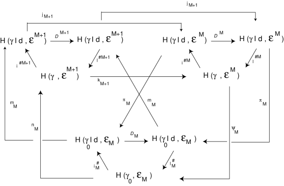
Figure 1: Exact triangle of exact triangles

References

- [1] C. Becchi, A. Rouet, and R. Stora, “Renormalization of gauge theories,” Annals Phys. 98 (1976) 287.
- [2] J. A. Dixon, “Cohomology and renormalization of gauge theories. 2,”. HUTMP 78/B64.
- [3] O. Piguet and S. P. Sorella, “Algebraic renormalization: Perturbative renormalization, symmetries and anomalies,” Lect. Notes Phys. M28 (1995) 1–134.
- [4] G. Bonneau, “Some fundamental but elementary facts on renormalization and regularization: A critical review of the eighties,” Int. J. Mod. Phys. A5 (1990) 3831–3860.
- [5] J. M. Figueroa-O’Farrill and S. Stanciu, “Nonsemisimple Sugawara constructions,” Phys. Lett. B327 (1994) 40–46, hep-th/9402035.
- [6] A. A. Tseytlin, “On gauge theories for nonsemisimple groups,” Nucl. Phys. B450 (1995) 231–250, hep-th/9505129.
- [7] F. Brandt, N. Dragon, and M. Kreuzer, “Completeness and nontriviality of the solutions of the consistency conditions,” Nucl. Phys. B332 (1990) 224–249.
- [8] F. Brandt, N. Dragon, and M. Kreuzer, “The gravitational anomalies,” Nucl. Phys. B340 (1990) 187–224.
- [9] M. Dubois-Violette, M. Henneaux, M. Talon, and C.-M. Viallet, “General solution of the consistency equation,” Phys. Lett. B289 (1992) 361–367, hep-th/9206106.
- [10] C. Chevalley and S. Eilenberg, “Cohomology theory of Lie groups and Lie algebras,” Trans. Amer. Math. Soc. 63 (1948) 85.
- [11] M. Postnikov, Leçons de géométrie: Groupes et algèbres de Lie. Editions Mir, 1985.
- [12] W. Greub, S. Halperin, and R. Vanstone, Connections, Curvature and Cohomology. Volume III: Cohomology of Principal Bundles and Homogeneous Spaces, vol. 47 of Pure and Applied Mathematics. A Series of Monographs and Textbooks. Academic Press, 1976.
- [13] F. Brandt, N. Dragon, and M. Kreuzer, “Lie algebra cohomology,” Nucl. Phys. B332 (1990) 250.
- [14] J. Wess and B. Zumino, “Consequences of anomalous Ward identities,” Phys. Lett. B37 (1971) 95.
- [15] M. Dubois-Violette, M. Talon, and C. M. Viallet, “New results on BRS cohomology in gauge theory,” Phys. Lett. 158B (1985) 231.
- [16] M. Dubois-Violette, M. Talon, and C. M. Viallet, “BRS algebras: Analysis of the consistency equations in gauge theory,” Commun. Math. Phys. 102 (1985) 105.
- [17] M. Talon, “Algebra of anomalies,”. Presented at Cargese Summer School, Cargese, France, Jul 15- 31, 1985.
- [18] M. Dubois-Violette, M. Talon, and C. M. Viallet, “Anomalous terms in gauge theory: Relevance of the structure group,” Ann. Poincare 44 (1986) 103–114.
- [19] R. Stora, “Algebraic structure and topological origin of anomalies,”. Seminar given at Cargese Summer Inst.: Progress in Gauge Field Theory, Cargese, France, Sep 1-15, 1983.
- [20] B. Zumino, Y.-S. Wu, and A. Zee, “Chiral anomalies, higher dimensions, and differential geometry,” Nucl. Phys. B239 (1984) 477–507.
- [21] B. Zumino, “Chiral anomalies and differential geometry,”. Lectures given at Les Houches Summer School on Theoretical Physics, Les Houches, France, Aug 8 - Sep 2, 1983.
- [22] J. Manes, R. Stora, and B. Zumino, “Algebraic study of chiral anomalies,” Commun. Math. Phys. 102 (1985) 157.
- [23] G. Hochschild and J. Serre, “Cohomology of Lie algebras,” Annals of Mathematics 57 (1953), no. 3,.
- [24] A. Achucarro and P. K. Townsend, “A Chern-Simons action for three-dimensional anti-de Sitter supergravity theories,” Phys. Lett. B180 (1986) 89.
- [25] E. Witten, “(2+1)-dimensional gravity as an exactly soluble system,” Nucl. Phys. B311 (1988) 46.
- [26] A. Vinogradov, “On the algebra-geometric foundations of Lagrangian field theory,” Sov. Math. Dokl. 18 (1977) 1200.
- [27] F. Takens, “A global version of the inverse problem to the calculus of variations,” J. Diff. Geom. 14 (1979) 543.
- [28] W. Tulczyjew, “The Euler-Lagrange resolution,” Lecture Notes in Mathematics 836 (1980) 22.
- [29] I. Anderson and T. Duchamp, “On the existence of global variational principles,” Amer. J. Math. 102 (1980) 781.
- [30] M. D. Wilde, “On the local Chevalley cohomology of the dynamical Lie algebra of a symplectic manifold,” Lett. Math. Phys. 5 (1981) 351.
- [31] T. Tsujishita, “On variational bicomplexes associated to differential equations,” Osaka J. Math. 19 (1982) 311.
- [32] P. Olver, Applications of Lie Groups to Differential Equations. Spinger Verlag, New York, 2nd ed., 1993. 1st ed., 1986.
- [33] R. Wald, “On identically closed forms locally constructed from a field,” J. Math. Phys. 31 (1990) 2378.
- [34] M. Dubois-Violette, M. Henneaux, M. Talon, and C.-M. Viallet, “Some results on local cohomologies in field theory,” Phys. Lett. B267 (1991) 81–87.
- [35] L. Dickey, “On exactness of the variational bicomplex,” Cont. Math. 132 (1992) 307.
- [36] M. Henneaux and B. Knaepen, “The Wess-Zumino consistency condition for p-form gauge theories,” Nucl. Phys. B548 (1999) 491, hep-th/9812140.
- [37] G. Barnich, F. Brandt, and M. Henneaux, “Local BRST cohomology in gauge theories,” Phys. Rept. 338 (2000) 439–569, hep-th/0002245.
- [38] S. P. Sorella, “Algebraic characterization of the Wess-Zumino consistency conditions in gauge theories,” Commun. Math. Phys. 157 (1993) 231–243, hep-th/9302136.
- [39] I. Anderson, “The variatonal bicomplex,” tech. rep., Formal Geometry and Mathematical Physics, Department of Mathematics, Utah State University, 1989.
- [40] G. Barnich and F. Brandt, “Covariant theory of asymptotic symmetries, conservation laws and central charges,” hep-th/0111246.
- [41] G. Barnich and M. Henneaux, “Consistent couplings between fields with a gauge freedom and deformations of the master equation,” Phys. Lett. B311 (1993) 123–129, hep-th/9304057.
- [42] M. Henneaux, “Consistent interactions between gauge fields: The cohomological approach,” in Secondary Calculus and Cohomological Physics, A. V. M. Henneaux, J. Krasil’shchik, ed., vol. 219 of Contemporary Mathematics, pp. 93–109. Amercian Mathematical Society, 1997. hep-th/9712226.
- [43] S.-T. Hu, Homotopy theory, vol. VIII of Pure and Applied Mathematics. A Series of Monographs and Textbooks. Academic Press, 1959.