Lorentz transformation and vector field flows

Abstract

The parameter changes resulting from a combination of Lorentz transformation are shown to form vector field flows. The exact, finite Thomas rotation angle is determined and interpreted intuitively. Using phase portraits, the parameters evolution can be clearly visualized. In addition to identifying the fixed points, we obtain an analytic invariant, which correlates the evolution of parameters.

I Introduction

One of the basic questions in the Lorentz transformation is velocity addition. Although algebraic formulas exist [1], the velocity transformations are quite complicated owing to their non-commutative nature. The conceptual complexity arises mainly from the counterintuitive consequences of the Thomas rotation. Furthermore, the determination of the transformation parameters is in general quite involved.

Interestingly, it has recently been shown [2] that the two-flavor neutrino mass matrix in the seesaw model [3] exhibits a Lorentz group-like structure, from which the constraint on the mixing angle and the hierarchical structure of the neutrino masses can be established. On the other hand, the RGE (Renormalization Group Equation) running of the neutrino mass and mixing angle between high and low energy scales can be illustrated as the flow of vector field [4]. In the literature, however, the link between Lorentz transformation and vector field flows has not been investigated even though there seems an inherent connection between them.

Following a general and intuitive approach, we shall analyze the flow-like structure of the Lorentz velocity transformation, and show that some intriguing results can be obtained directly along this line. Starting from the simple commutation relations of the $2\times 2$ spinor algebra, we first construct the Lorentz velocity transformation and obtain the exact, finite Thomas rotation angle associated with the transformation. This approach leads directly to an alternative physical interpretation of the Thomas rotation angle. We then derive and solve the differential equations for the transformation parameters and illustrate their properties in the phase portraits. In particular, an invariant governing the evolution of velocity and direction in the Lorentz velocity addition is established from our results. As an example, the collimation effect of the relativistic decay is interpreted as the approach to a fixed point in a vector field flow problem.

II Lorentz velocity transformation

The order of successive Lorentz transformations plays a crucial role when two inertial reference frames are related. This property is indicated by the commutation relations [5]:

$$[J_{i},J_{j}] =i\epsilon_{ijk}J_{k},$$ (1)

$$[J_{i},K_{j}] =i\epsilon_{ijk}K_{k},$$ (2)

$$[K_{i},K_{j}] =-i\epsilon_{ijk}J_{k},$$ (3)

where $J_{i,j,k}$ and $K_{i,j,k}$ are the infinitesimal generators of rotations and pure Lorentz boosts, respectively. The Thomas precession is known to originate from this non-commutability of the generators: A new reference frame reached by two successive Lorentz boosts cannot be reached by a third, pure boost from the original frame without a Thomas rotation. In the literature, the infinitesimal Thomas rotation angle is usually calculated from a continuous application of infinitesimal Lorentz transformations consisting of rotations and boosts [1], while the finite Thomas rotation angle can be determined by a variety of approaches [6, 7, 8]. In this article we employ the simple properties of Pauli matrices instead, for the determination of finite Thomas rotation angle as well as other parameters in the Lorentz velocity transformations.

It is well known that $J_{i}=\sigma_{i}/2$ (rotations) and $K_{i}=i\sigma_{i}/2$ (boosts) are two-dimensional representations of the Lorentz group: A finite rotation about an arbitrary axis $\hat{n}$ through an angle $\Theta$ is written as $\mathbf{R}$ = $\exp(\frac{i\Theta\vec{\sigma}\cdot\hat{n}}{2})$, while $\mathbf{B}$ = $\exp(\frac{-\kappa\vec{\sigma}\cdot\hat{n}}{2})$ represents a pure boost along an arbitrary direction $\hat{n}$, with $\kappa$ the rapidity parameter. Without loss of generality, we consider the addition of two pure boosts by choosing one boost of rapidity parameter $\eta$ along the direction $\hat{n}_{\theta_{0}}=(\sin\theta_{0}\hat{x}+\cos\theta_{0}\hat{z})$:

$$\mbox{\boldmath$\beta_{1}$}=\tanh\eta(\sin\theta_{0}\hat{x}+\cos\theta_{0}\hat{z}),$$ (4)

and the other of rapidity $\xi$ along $\hat{z}$:

$$\mbox{\boldmath$\beta_{2}$}=\tanh\xi\hat{z},$$ (5)

as shown in Fig.1. The combination of the two pure boosts

$$L=e^{-\frac{\xi}{2}\vec{\sigma}\cdot\hat{z}}e^{-\frac{\eta}{2}\vec{\sigma}\cdot\hat{n}_{\theta_{0}}}=e^{-\frac{\xi}{2}\sigma_{3}}e^{-\frac{\eta}{2}(\sigma_{3}\cos\theta_{0}+\sigma_{1}\sin\theta_{0})}$$ (6)

is equivalent to a third boost plus a rotation about an axis parallel to $\hat{y}$:

$$L = e^{-\frac{\lambda}{2}(\sigma_{3}\cos\theta+\sigma_{1}\sin\theta)}e^{i\frac{\tau}{2}\sigma_{2}}$$ (7)

$$= e^{-i\frac{\theta}{2}\sigma_{2}}e^{-\frac{\lambda}{2}\sigma_{3}}e^{i\frac{\theta+\tau}{2}\sigma_{2}},$$ (8)

where $\tau$ is the Thomas rotation angle and $\lambda$ represents the third rapidity in the direction $\hat{n}_{\theta}=(\sin\theta\hat{x}+\cos\theta\hat{z})$, with $0\leq\theta\leq\pi$. Given two boosts of parameters $\xi$ and $\eta$, which are separated by an angle $\theta_{0}$, the new parameters associated with the third boost, $\lambda$ and $\theta$, can be derived from the simple product $LL^{T}$ [2]:

$$\tan\theta=\frac{\sin\theta_{0}\sinh\eta}{\sinh\xi\cosh\eta+\cos\theta_{0}\cosh\xi\sinh\eta},$$ (9)

$$\cosh\lambda=\cosh\xi\cosh\eta+\cos\theta_{0}\sinh\xi\sinh\eta.$$ (10)

The above two equations are equivalent to eq.(11.32) in Jackson [1].

III The Thomas rotation angle

To determine the finite Thomas rotation angle $\tau$, we now consider $L^{T}L$. From eq.(4),

$$L^{T}L=e^{-\frac{\eta}{2}(\sigma_{3}\cos\theta_{0}+\sigma_{1}\sin\theta_{0})}e^{-\xi\sigma_{3}}e^{-\frac{\eta}{2}(\sigma_{3}\cos\theta_{0}+\sigma_{3}\sin\theta_{0})},$$ (11)

while eq.(5) gives

$$L^{T}L=e^{-i\frac{\theta+\tau}{2}\sigma_{2}}e^{-\lambda\sigma_{3}}e^{i\frac{\theta+\tau}{2}\sigma_{2}}.$$ (12)

Eq.(8) can further be simplified by using the identity

$$e^{-i\frac{\theta_{0}}{2}\sigma_{2}}e^{-\frac{\eta}{2}\sigma_{3}}e^{i\frac{\theta_{0}}{2}\sigma_{2}}=e^{-\frac{\eta}{2}(\sigma_{3}\cos\theta_{0}+\sigma_{1}\sin\theta_{0})},$$ (13)

which leads to

$$L^{T}L=e^{-i\frac{\theta_{0}}{2}\sigma_{2}}(e^{-\frac{\eta}{2}\sigma_{3}}e^{-\xi\sigma_{(-\theta_{0})}}e^{-\frac{\eta}{2}\sigma_{3}})e^{i\frac{\theta_{0}}{2}\sigma_{2}},$$ (14)

where $\sigma_{(-\theta_{0})}\equiv\sigma_{3}\cos(-\theta_{0})+\sigma_{1}\sin(-\theta_{0})$. Eqs.(9) and (11) lead to a simple relation:

$$\tan(\theta+\tau-\theta_{0})\equiv\tan\phi=\frac{-\sin\theta_{0}\sinh\xi}{\cosh\xi\sinh\eta+\cos\theta_{0}\sinh\xi\cosh\eta}.$$ (15)

Here, $\phi$ specifies the direction of the resultant third boost when $\beta_{1}$ and $\beta_{2}$ are applied in a reverse order. The finite Thomas rotation angle is then given by

$$\tan\tau=\frac{\tan\phi+\tan(\theta_{0}-\theta)}{1-\tan\phi\tan(\theta_{0}-\theta)}.$$ (16)

Eqs.(6), (7), and (13) are exact, and valid for the finite Lorentz transformations. In the limit of infinitesimal Lorentz transformation, we may consider a finite boost $\beta_{1}=\tanh\eta$, followed by an infinitesimal boost $\beta_{2}=\tanh(\Delta\xi)\cong\Delta\xi$. The infinitesimal Thomas rotation angle then becomes

$$\Delta\tau\cong\frac{\sin\theta_{0}}{\sinh\eta}(\cosh\eta-1)\Delta\xi,$$ (17)

which agrees with the result in Section 11.8 of Ref. [1]. Note that our notations are slightly different from that of Ref. [1]: our $\beta_{1}$ and $\beta_{2}$ correspond to $\beta$ and $\gamma^{2}\delta\mbox{\boldmath$\beta_{\parallel}$}+\gamma\delta\mbox{\boldmath$\beta_{\perp}$}$ in Ref. [1], respectively. We also note that eq.(13) agrees with eq.(37) of Ref. [8] up to an overall sign, which is due merely to the different sense of rotation.

An alternative physical interpretation of the Thomas rotation angle becomes clear from our formulation as we examine two boosts combined in reverse orders. From eq.(4) and eq.(5),

$$e^{-\frac{\xi}{2}\sigma_{3}}e^{-\frac{\eta}{2}\sigma_{\theta_{0}}}=e^{-\frac{\lambda}{2}\sigma_{\theta}}e^{i\frac{\tau}{2}\sigma_{2}},$$ (18)

where $\sigma_{\theta_{0}}\equiv\sigma_{3}\cos\theta_{0}+\sigma_{1}\sin\theta_{0}$, and $\sigma_{\theta}\equiv\sigma_{3}\cos\theta+\sigma_{1}\sin\theta$. It follows that

$$e^{-\frac{\xi}{2}\sigma_{3}}e^{-\frac{\eta}{2}\sigma_{\theta_{0}}}e^{-i\frac{\tau}{2}\sigma_{2}}=e^{-\frac{\lambda}{2}\sigma_{\theta}}.$$ (19)

Since $\sigma_{\theta}$ is symmetric, it follows that

$$e^{i\frac{\tau}{2}\sigma_{2}}(e^{-\frac{\eta}{2}\sigma_{\theta_{0}}}e^{-\frac{\xi}{2}\sigma_{3}})e^{i\frac{\tau}{2}\sigma_{2}}=e^{-\frac{\xi}{2}\sigma_{3}}e^{-\frac{\eta}{2}\sigma_{\theta_{0}}}.$$ (20)

Eq.(17) implies that the combination of two boosts, $\exp(-\frac{\xi}{2}\sigma_{3})\exp(-\frac{\eta}{2}\sigma_{\theta_{0}})$, is related to its reverse, $\exp(-\frac{\eta}{2}\sigma_{\theta_{0}})\exp(-\frac{\xi}{2}\sigma_{3})$, by two identical rotations, $e^{i\frac{\tau}{2}\sigma_{2}}$. In other words, operating a rotation on a reference frame before and after two successive boosts would bring this frame to the same reference frame that is reached by the same two boosts operated in reverse order. The angle associates with this particular rotation is the Thomas rotation angle, whose existence is thus directly related to the non-commutativity of the Lorentz transformations.

IV Lorentz transformations and vector field flows

A geometrical visualization of the Lorentz transformation can be realized as a vector field flow problem. Let us start from any Lorentz transformation specified by the parameters $(\theta,\beta,\tau)$, which we denote as $L_{(\theta,\beta,\tau)}$. A second infinitesimal boost would change $L$ according to $L_{d\xi}L_{(\theta,\beta,\tau)}=L_{(\theta+d\theta,\beta+d\beta,\tau+d\tau)}$. Clearly, this change can be represented as an infinitesimal vector in a 3D space originating from the $(\theta,\beta,\tau)$ point. The general problem for arbitrary $\xi$ and $(\theta,\beta,\tau)$ is thus succinctly described by a vector field flow problem.

To quantify the vector flows we need three differential equations for $\theta$, $\beta$ ($\beta\equiv\tanh\lambda$), and $\tau$ which can be derived from eqs.(6), (7), and (13):

$$\frac{d\theta}{d\xi}=\frac{-\sin\theta}{\beta},$$ (21)

$$\frac{d\beta}{d\xi}=\cos\theta(1-\beta^{2}),$$ (22)

$$\frac{d\tau}{d\xi}=\frac{\sin\theta}{\beta}(1-\sqrt{1-\beta^{2}}).$$ (23)

We first examine the relation between the two angles, $\theta$ and $\tau$. From eq.(20) we see that at small $|\mbox{\boldmath$\beta$}|$, the Thomas rotation angle $\tau$ does not vary significantly with $\xi$: $\frac{d\tau}{d\xi}\approx 0$, while $\theta$ varies rapidly according to eq.(18). On the other hand, $\frac{d\theta}{d\xi}$ slows down and $\frac{d\tau}{d\xi}$ speeds up as $|\mbox{\boldmath$\beta$}|$ increases. From eqs.(18) and (20) we have

$$\frac{d\tau}{d\theta}=-(1-\sqrt{1-\beta^{2}}).$$ (24)

The solution, given by

$$\tau-\tau_{0}=\frac{1-\cosh\lambda}{\cosh\lambda}(\theta-\theta_{0}),$$ (25)

clearly describes the variation of $\tau$ and $\theta$ for a given boost $\beta$. For a given $|\mbox{\boldmath$\beta$}|$, eq.(18) implies that the rate of change of $\theta$ is maximum at $\theta=\pi/2$, where the two boosts are perpendicular. In addition, eqs.(12) and (13) imply that if $\beta_{1}\approx 1$ and $\beta_{2}\approx 1$, then $\tan\phi\cong 0$ and $\tau\cong\theta_{0}$. Therefore, when the two successive boosts are each close to light speed, the value of Thomas rotation angle associated with the transformation approaches that of the angle between the two boosts. Furthermore, $\tau=0$ if the two successive boosts are co-linear.

As for $\tau$ and $\lambda$, eqs.(19) and (20) give rise to the equation

$$\frac{d\tau}{d\beta}=\frac{\tan\theta(1-\sqrt{1-\beta^{2}})}{\beta(1-\beta^{2})},$$ (26)

with the solution given by

$$\tan\theta=\frac{\tau-\tau_{0}}{\ln(\cosh\lambda-1)-\ln(\cosh\lambda_{0}-1)},$$ (27)

which relates the change of Thomas angle to the boost parameters for a given angle $\theta$.

Finally, from eqs.(18) and (19) we have

$$\frac{d\theta}{d\beta}=\frac{-\tan\theta}{\beta(1-\beta^{2})}.$$ (28)

The solution is given by

$$\sin\theta\sinh\lambda=\sin\theta_{0}\sinh\lambda_{0}.$$ (29)

Interestingly, this solution represents an invariant that correlates the evolution of direction and magnitude of the resultant boost. Note that the Thomas rotation angle $\tau$ does not take part in this invariant. We also note that in the analysis of neutrino parameters [2], $\theta$ and $e^{2\lambda}$ represent the mixing angle and the physical neutrino mass ratio, respectively.

Our results can be illustrated clearly using the phase portraits. The $\theta-\beta$ phase portrait is shown in Fig.2, where the direction fields are plotted for increasing $\xi$ and the arrows are tangent to the trajectories. There are four fixed points for the evolution equations, eqs.(18) and (19): $(\beta,\theta)=(1,0)$, $(-1,\pi)$, $(1,\pi)$, and $(-1,0)$. The stability [10] of the fixed points as $\xi$ increases are determined by the eigenvalues of the Jacobian. Of the four fixed points, $(1,0)$ and $(-1,\pi)$ are stable (attractive) and the evolution of $\theta$ and $\beta$ is always toward one of the two points. On the other hand, the evolution is always directed away from the unstable (repulsive) fixed points, $(1,\pi)$ and $(-1,0)$. Note that the two attractive fixed points are physically identical, so are the two repulsive fixed points. This is because $\beta$ of opposite signs simply represent boosts in opposite directions. The phase portrait illustrates the following features:

(I). As $\xi$ increases, starting from any initial condition $(\beta_{0},\theta_{0})$, the values $(\beta,\theta)$ evolve along trajectories defined by the invariant, eq.(26). As $\xi\rightarrow\infty$, all of these trajectories converge onto the stable fixed points $(\beta,\theta)=(1,0)$ or $(-1,\pi)$, depending on the signs of the boosts. Thus, the resultant boost $\beta$ tends to evolve from its initial value toward $|\mbox{\boldmath$\beta$}|=1$ (extreme relativistic limit), and its direction evolves toward that of the second boost $\beta_{2}$. The evolution of direction also can be understood from eq.(18): $\frac{d\theta}{d\xi}\geq 0$ for a negative $\beta$ and $\frac{d\theta}{d\xi}\leq 0$ for a positive $\beta$.

(II). The long arrows with slopes approaching infinity near the region of small $|\mbox{\boldmath$\beta$}|$ and large $\sin\theta$ ($\theta\approx\pi/2$) represent the rapid variation of $\beta$’s direction in this region. This property is also implied by eq.(18).

(III). For $|\mbox{\boldmath$\beta$}|=1$, the slope of the trajectory becomes infinity and the transformation does not exist. Physically, this feature can be interpreted as no transformation from the rest frame of a photon to a laboratory frame.

It should be noted that the fixed point structure described above has a direct realization in the physical process of relativistic particle decays, e.g., $\pi^{0}\rightarrow\gamma\gamma$. For fast moving $\pi^{0}$ ($\xi\rightarrow\infty$), most photons (with ($\beta_{0},\theta_{0}$) in the rest frame) are focused in the forward direction (with $\beta\rightarrow 1$) in the lab frame. This can be clearly visualized in Fig.2, so that the vector field flow corresponds to the well-known collimation effect of relativistic decays. What is not so well-known, however, is that, during the collimation, there is a simple correlation between the direction ($\theta$) and the rapidity ($\lambda$), given in eq.(26).

The evolution of $\beta$, $\theta$, and $\tau$ can be visualized in a 3-D phase portrait. In Fig.3 the initial conditions corresponding to $\beta_{2}=0$ and arbitrary $(\beta_{1},\theta_{0})$ lie in the plane specified by $\tau=0$. As $\beta_{2}$ increases, $\theta$ and $\beta$ evolve along one of the trajectories in Fig.2 while changing the corresponding $\tau$ value at varying rates. This rate of change of $\tau$ is determined by the local values of $\beta$ and $\theta$ as implied by eq.(20). If the initial $\beta_{2}$ is chosen to be nonzero, the initial conditions lie in a plane specified by a nonzero $\tau$.

V Summary

Simple properties of the spinor algebra provide a general and effective solution to the problems of finite Lorentz velocity transformations. In particular, we found the exact solution of the finite Thomas rotation angle. It has an intuitive physical interpretation, directly related to the non-commutativity of Lorentz transformations. Following this line, we then treat the Lorentz velocity transformation as a vector field flow problem. In relating the two, we present the analytical results, eqs.(22), (24) and (26), which come directly from a set of differential equations, eqs.(18), (19), and (20). In addition, we show that the general features of the Lorentz transformation and the evolution of the parameters can be clearly visualized using the phase portraits of the parameters. The attractive fixed point of the vector field flow describes geometrically the well-known collimation effect of relativistic decays. The flow toward the fixed point follows trajectories given by the invariant, eq.(26).

As a final remark, we note that the invariant, eq.(26), carries the same form as the general, complex RGE invariant [4]. However, unlike the running of RGEs for the general neutrino mass matrix, in which the relative phase of the mass eigenvalues is nonzero and the evolution depends sensitively on the choice of initial conditions, the Lorentz velocity transformation corresponds to a vanishing relative phase and the evolution of parameters is not as sensitive to the initial conditions, i.e., physically there is only one attractive fixed point and one repulsive fixed point.

FIG. 1.: The combination of two boosts, $\beta_{1}$ and $\beta_{2}$, is equivalent to a third boost $\beta$ plus a rotation about $\hat{y}$.

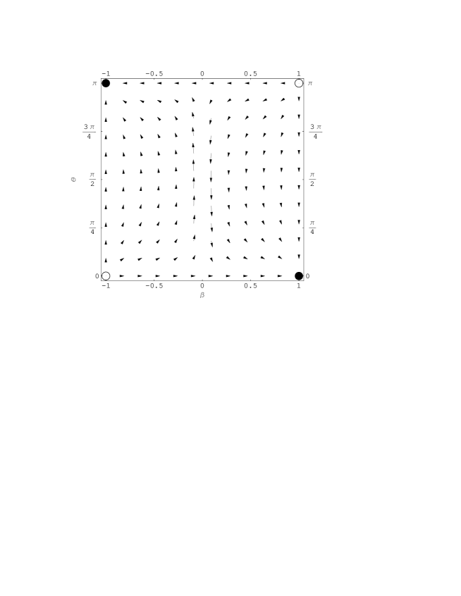
FIG. 2.: The $\theta-\beta$ phase portrait. All trajectories evolve toward either $(\beta,\theta)=(1,0)$ or $(\beta,\theta)=(-1,\pi)$. Note that a negative $\beta$ represents a boost in the direction opposite to that of a positive $\beta$. The trajectories are described by eq.(26); the attractive and repulsive fixed points are shown in the figure as $\bullet$ and $\circ$, respectively. Also note that we have used $\beta$ here in the graph instead of $\lambda$.

FIG. 3.: The evolution of $\beta$, $\theta$, and $\tau$. Note that as $\beta\rightarrow 1$, $(\theta,\tau)$ approaches $(0,\pi)$ for $\beta>0$ and that $(\theta,\tau)$ approaches $(\pi,-\pi)$ for $\beta<0$. Fig.2 corresponds to a “slice” of this figure at a particular $\tau$ value. The rate of change of $\tau$ with respect to $\xi$ depends on the local values of $\beta$ and $\theta$.

- [1] J. D. Jackson, Classical Electrodynamics (2nd Edition), John Wiley & Sons (1975), Chapter 11.
- [2] T. K. Kuo, G.-H. Wu, and S.-H. Chiu , Phys. Rev. D62, 051301 (2000), hep-ph/0003066; T. K. Kuo, S.-H. Chiu, and G.-H. Wu, Eur. Phys. J. C21, 281-289 (2001), hep-ph/0011058.
- [3] M. Gell-Mann, P. Ramond, and R. Slansky, in Supergravity, eds. P. van Nieuwenhuizen and D. Freeman, North Holland, Amsterdam (1979); T. Yanagida, in Proceedings of the Workshop on the Unified Theory and Baryon Number in the Universe. eds. O. Sawada and A. Sugamoto, KEK (1979).
- [4] See, e.g., T. K. Kuo, J. Pantaleone, and G.-H. Wu, Phys. Lett. B528, 101 (2001), hep-ph/0104131, and the references therein.
- [5] See, e.g., L. H. Ryder, Quantum Field Theory, Cambridge University Press (1985).
- [6] A. J. MacFarlane, J. Math. Phys. 3, 1116-1129 (1962).
- [7] H. Urbantke, Am. J. Phys. 58, 747 (1990).
- [8] A. A. Ungar, Am. J. Phys. 59, 824 (1991).
- [9] C. Misner, K. Thorne, and J. Wheeler, Gravitation, W. H. Freeman and Company (1975), Chapter 41.
- [10] S. Strogatz, Nonlinear Dynamics and Chaos (1994), Perseus Publishing, Cambridge, Massachusetts.