On the Remarkable Spectrum of a Non-Hermitian Random Matrix Model

Abstract

A non-Hermitian random matrix model proposed a few years ago has a remarkably intricate spectrum. Various attempts have been made to understand the spectrum, but even its dimension is not known. Using the Dyson-Schmidt equation, we show that the spectrum consists of a non-denumerable set of lines in the complex plane. Each line is the support of the spectrum of a periodic Hamiltonian, obtained by the infinite repetition of any finite sequence of the disorder variables. Our approach is based on the “theory of words.” We make a complete study of all 4-letter words. The spectrum is complicated because our matrix contains everything that will ever be written in the history of the universe, including this particular paper.

I A Class of Non-Hermitian Random Matrix Models

Some time ago, Feinberg and one of us (in a paper to be referred to as FZ FZ ) proposed the study of the equation

$$\psi_{k+1}+r_{k-1}\psi_{k-1}=E\psi_{k}$$ (1)

where the real numbers $r_{k}$ are generated from some random distribution. Two particularly simple models were studied: (A) the $r_{k}$’s are equal to $\pm 1$ with equal probability, and (B) $r_{k}=e^{i\theta_{k}}$ with the angle $\theta_{k}$ uniformly distributed between $0$ and $2\pi.$

Imposing the boundary condition $\psi_{0}=\psi_{N+2}=0$ on (1) we can write the set of equations as the eigenvalue equation

$$H_{N}\psi=E\psi$$ (2)

with $\psi$ the column eigenvector with components $\{\psi_{1},$ $\psi_{2},$ $\cdots,$ $\psi_{N},$ $\psi_{N+1}\}$ and $H_{N}$ the $(N+1)$ by $(N+1)$ non-Hermitian random matrix

$$H_{N}=\left(\begin{array}[]{llllll}0&1&0&&&\\ r_{1}&0&1&0&&\\ 0&r_{2}&0&1&0&\\ &0&\ddots&\ddots&\ddots&0\\ &&0&r_{N-1}&0&1\\ &&&0&r_{N}&0\end{array}\right)$$

While quantum mechanics is of course Hermitian it is convenient to think of $H$ as a Hamiltonian and (1) as the non-Hermitian Schrödinger equation describing the propagation of a particle hopping on a 1-dimensional lattice.

Some applications of non-Hermitian random Hamiltonians include vortex line pinning in superconductors 1 ; 2 ; fz2 and growth models in population biology 4 . A genuine localization transition can occur for random non-Hermitian Schrödinger Hamiltonians 5 ; 6 ; 7 ; 8 ; 9 ; 10 ; 11 ; 12 in one dimension.

As mentioned in FZ, with the open chain boundary condition $\psi_{0}=\psi_{N+2}=0$ the more general equation

$$s_{k+1}\psi_{k+1}+r_{k-1}\psi_{k-1}=E\psi_{k}$$ (3)

can always be reduced to (1) by an appropriate “gauge” transformation $\psi_{k}\rightarrow\lambda_{k}\psi_{k}.$ Furthermore, applying the transformation $\psi_{k}\rightarrow u^{-k}\psi_{k}$ to (1) we see that if we change $r_{k}\rightarrow u^{2}r_{k}$ then the spectrum changes by $E\rightarrow uE.$ Thus, scaling the magnitude of the $r_{k}$’s merely stretches the spectrum, and flipping the sign of all the $r_{k}$’s corresponds to rotating the spectrum by $90^{0}.$

It is also useful to formulate the problem in the transfer matrix formalism. Write (1) as

$$\left(\begin{array}[]{l}\psi_{k+1}\\ \psi_{k}\end{array}\right)=T_{k-1}\left(\begin{array}[]{l}\psi_{k}\\ \psi_{k-1}\end{array}\right)$$ (4)

where the transfer matrix $T_{k}$ is defined as the 2 by 2 matrix

$$T_{k}=\left(\begin{array}[]{ll}E&-r_{k}\\ 1&0\end{array}\right)$$ (5)

Define $P\equiv T_{N}T_{N-1}\cdots T_{2}T_{1}.$ Then the boundary condition implies

$$EP_{11}+P_{12}=0$$ (6)

The solution of this polynomial equation in $E$ determines the spectrum.

Since $H$ is non-Hermitian the eigenvalues invade the complex plane. For model B, the spectrum has an obvious rotational symmetry and forms a disk (see Fig. 1, which displays the support of the density of states).

Figure 1: Support of the density of states for model B.

An expansion of the density of eigenvalues around $E=0$ to very high orders in $E$ has been given by Derrida et al. derrida . This analytic expansion however cannot predict singularities in the density of states.

In contrast, for model A the spectrum enjoys only a rectangular $Z_{2}\otimes Z_{2}$ symmetry. The first $Z_{2}$ corresponds to $E\rightarrow E^{\ast}$ obtained by complex conjugating the eigenvalue equation $H\psi=E\psi.$ The second $Z_{2}$ corresponds to $E\rightarrow-E$ obtained by the bipartite transformation $\psi_{k}\rightarrow(-)^{k}\psi_{k}.$ Remarkably, FZ found that the spectrum has an enormously complicated fractal-like form. In Fig. 2 we plot the support of the density of eigenvalues in the complex plane for a $4000\times 4000$ matrix, for a specific realization of the disorder.

Figure 2: Support of the density of states for model A for a $4000\times 4000$ matrix and a single realization of disorder.

In Fig. 3 we plot the support of the density of states in the complex plane for a $1000\times 1000$ matrix, averaged over 100 realizations of the disorder.

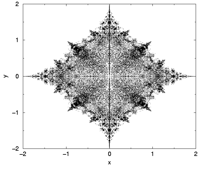
Figure 3: Support of the density of states for model A for a $1000\times 1000$ matrix averaged over 100 realizations of disorder.

Contrasting Figs. 2 and 3 with Fig. 1, one can see why it has been a challenge for mathematical physicists to understand the nature of the spectrum.

II Basic Formalism

In general, for random non-Hermitian matrices $H$, the density of eigenvalues can be obtained by

$$\rho(x,y)=\frac{1}{\pi}\frac{\partial}{\partial z^{\ast}}G(z,z^{\ast})$$ (7)

where the Green’s function is defined by

$$G(z,z^{\ast})=\left\langle{\frac{1}{N}\mathrm{tr}\frac{1}{z-H}}\right\rangle$$

with the bracket denoting averaging and $z=x+iy$ (see, for example, ref. 8 for a proof of these relations). Equation (7) follows from the identity

$$\frac{\partial}{\partial z^{\ast}}\frac{\partial}{\partial z}\mathrm{log}\text{ }z=\frac{\partial}{\partial z^{\ast}}\frac{1}{z}=\pi\,\delta(x)\,\delta(y)$$ (8)

where $z=x+iy$. Expanding $G(z,z^{\ast})=\frac{1}{z}\sum_{k=0}^{\infty}{z^{-k}}\left\langle{\frac{1}{N}\mathrm{tr}H^{k}}\right\rangle$ we see that $\left\langle{\frac{1}{N}\mathrm{tr}H^{k}}\right\rangle$ counts the number of paths of a particle returning to the origin in $k$ steps.

Evidently, for model A each link has to be traversed 4 times. The spectrum of model A was studied by Cicuta et al. cicuta and by Gross and one of us GZ by counting paths. In particular, Cicuta et al. gave an explicit expression for the number of paths. Recently, the more general problem of even-visiting random walks has been studied extensively (see ref. Bau ). In addition, exact analytic results for the Lyapunov exponent have been found by Sire and Krapivsky sire .

In this paper we propose a different approach based on the theory of words. We will focus on model A although some of our results apply to the general class of models described by (3).

One important issue is the dimensionality of the spectrum of model A. In general, the spectrum of non-Hermitian random matrices when averaged over the randomness is 2-dimensional (for example, the spectrum of model B). Many of the authors who have looked at model A believe that its spectrum, as shown in Figs. 2 and 3, is quasi-0-dimensional: the spectrum seems to consist of many accumulation points. Here we claim that the dimension of the spectrum actually lies between $1$ and $2$ dimensions, in the sense described below.

III Distribution of the Characteristic Ratio

Consider the degree $(N+1)$ characteristic polynomial $\Delta_{N+1}(z)\equiv\mathrm{\det}(H_{N}+zI_{N+1})$, where $I_{N+1}$ denotes the $(N+1)\times(N+1)$ identity matrix. We easily obtain the recursion relation

$$\Delta_{N+1}(z)=z\Delta_{N}(z)-r_{N}\Delta_{N-1}(z)$$

with $\Delta_{0}(z)=1$ and $\Delta_{1}(z)=z.$ Note that this second order recursion relation can be expressed in terms of transfer matrices as

$$\left(\begin{array}[]{c}\Delta_{N+1}(z)\\ \Delta_{N}(z)\end{array}\right)=\left(\begin{array}[]{cc}z&-r_{N}\\ 1&0\end{array}\right)\left(\begin{array}[]{c}\Delta_{N}(z)\\ \Delta_{N-1}(z)\end{array}\right)$$ (9)

very similar to those defined for the wave function $\psi$, with the transfer matrix given by

$$U_{N}=\left(\begin{array}[]{cc}z&-r_{N}\\ 1&0\end{array}\right).$$ (10)

Following Dyson and Schmidt Dyson ; Schmidt we consider the characteristic ratio

$$y_{k}(z)\equiv\frac{\Delta_{k}(z)}{\Delta_{k-1}(z)},$$ (11)

which satisfies the recursion relation

$$y_{k+1}=z-\frac{r_{k}}{y_{k}}$$ (12)

with initial condition $y_{1}=z$.

The hope is that, while the characteristic polynomials $\Delta_{k}(z)$ obviously changes dramatically as $k$ varies, the characteristic ratio $y_{k}(z)$ might converge asymptotically.

From the definition in eq. (11), it is clear that a point $z$ is in the spectrum of the $N\times N$ matrix iff $y_{N}(z)=0$ and $y_{N+1}(z)=\infty$. Thus a point $z$ belongs to the spectrum if the corresponding set of variables $\{y_{N}\}$ is unbounded, that is, if the probability of escape of the variable $y_{n}$ to $\infty$ is finite. As is shown in Bau , this condition is sufficient to determine the spectrum along the real axis ($z\in R$), but is insufficient in the complex case.

Let $P_{k}(y_{k})$ be the probability distribution of $y_{k}$ (note that $y_{k}$ is complex). Then

$$P_{k+1}(y_{k+1})=\left\langle{\int d^{2}y_{k}\,P_{k}(y_{k})\delta^{(2)}(y_{k+1}-z+\frac{r_{k}}{y_{k}})}\right\rangle$$

where the brackets denote the average over the disorder variables $\{r_{k}\}$. In the thermodynamic limit $k\rightarrow\infty$, under fairly general conditions osedelec it can be shown that the probability distribution has a limit $P(y)$, called the invariant distribution, which is determined by the self-consistent equation

$$P(y) = \left\langle{\int\,d^{2}t\,P(t)\delta^{(2)}(y-z+\frac{r}{t})}\right\rangle$$

$$= \left\langle{\frac{\mid r\mid^{2}}{\mid z-y\mid^{4}}P(\frac{r}{z-y})}\right\rangle,$$

where we have used the fact that $\delta^{(2)}(f(z))$ near a zero, $z_{0}$, of $f(z)$ is given by $\delta^{(2)}(z-z_{0})\,|\frac{df}{dz}|^{-2}$.

For model A, we obtain the amusing equation

$$P(y)=\frac{1}{2\mid z-y\mid^{4}}\left(P({\frac{1}{z-y}})+P({\frac{-1}{z-y}})\right).$$ (13)

This type of equation has been studied extensively for the real case in aeppli ; orland ; luck . It can be shown that it can be solved by the Ansatz

$$P(y)=\sum_{j}a_{j}\delta^{(2)}(y-b_{j}(z)),$$ (14)

where the $b_{j}$’s depend on $z$ whereas the $a_{j}$’s don’t. Note that the index $j$ is not necessarily an integer and can refer to a continuous set. In addition, it can be shown that the $b_{j}(z)$ are the stable fixed points of the product of any sequence of transfer matrices $U$ (see the next section).

Plugging (14) into (13) we have

$$\sum_{j}a_{j}\delta^{(2)}(y-b_{j})=\frac{1}{2}\sum_{j}a_{j} \!\!\!\!\!\!\{\delta^{(2)}(y-z+\frac{1}{b_{j}})$$

$$+\delta^{(2)}(y-z-\frac{1}{b_{j}})\}.$$

Since the right hand side has twice as many delta function spikes as the left hand side, for the two sides to match we expect that, in general, the index $j$ would have to run over an infinite set.

For a given complex number $z$, we demand that the two sets of complex numbers $\{b_{j}\}$ and $\{z-1/b_{j},z+1/{b_{j}}\}$ be the same. This very stringent condition should then determine the $\{b_{j}(z)\}.$

To see how this works, focus on a specific $b_{1}$ (Since the label $j$ has not been specified this can represent any $b_{j}$). It is equal to either $z-{1}/{b_{2}}$ or $z+{1}/{b_{2}}$ for some $b_{2}.$ But $b_{2}$ must in its turn be equal to either $z-{1}/{b_{3}}$ or $z+{1}/{b_{3}}$ for some $b_{3}$. This process of identification must continue until we return to $b_{1}$. Indeed, if the process of return to $b_{1}$ occurs in a finite number $L$ of steps, then it will repeat indefinitely (since the system is back at its starting point $b_{1})$. It is this infinite repetition which gives a finite weight to the $\delta-$function at $b_{1}$. By contrast, if the number of steps needed to return to the initial point $b_{1}$ is infinite, then the weight associated with this point vanishes, and it will not be present in the spectrum.

We thus conclude that the support of the distribution of $P(y)$ is the closure of the set of all the stable fixed points of the product of any sequence of transfer matrices $U$. We also conclude that the support of the density of states of the non-Hermitian matrix, in the thermodynamic limit, is given by the zeroes of any stable fixed point: $b_{j}(z)=0$. What is important to notice is that the $a_{j}$ are independent of $z$ and depend only on the length of the word. Thus, we conclude that the set of complex numbers $\{b_{j}(z)\}$ is determined by the solution of an infinite number of fixed point equations.

IV The Theory of Words

It is useful here to introduce the theory of words. A word $w$ of length $L$ is defined as the sequence $\{w_{1},w_{2},\cdots,w_{L}\}$ where the letters $w_{j}=\pm 1$. In other words, we have a binary alphabet. Let us also define the repetition of a given word a specific number of times as a simple sentence. We can then string together simple sentences to form paragraphs.

For a given word $w$ of length $L$, consider a function $f_{L}(b;z,w)$ to be constructed iteratively. For notational simplicity we will suppress the dependence of $f_{L}$ on $b,$ $z,$ and $w,$ indicating only its dependence on the length $L$ of the word $w.$ The iteration begins with

$$f_{1}=z-\frac{w_{1}}{b}$$

and continues with

$$f_{j+1}=z-\frac{w_{j+1}}{f_{j}}.$$ (15)

We define $f(b;z,w)\equiv f_{L}.$

The set of complex numbers $\{b_{j}(z)\}$ are then determined as follows. Consider the set of all possible words. For each word $w$, determine the solution of the fixed point equation

$$b=f(b;z,w).$$

By considering small deviations from the solution, we see that the solution is a stable fixed point only if

$$\left|\frac{\partial f(b;z,w)}{\partial b}\right|<1.$$ (16)

The set of all possible words $w$ generates the set of complex numbers $\{b_{j}(z)\}.$ In other words, $b$ is determined by a continued fraction equation, since

$$f(b;z,w)=z-\frac{w_{L}}{z-\frac{w_{L-1}}{z-\frac{w_{L-2}}{\frac{\ddots}{z-\frac{w_{1}}{b}}}}}.$$

We see that $f_{j}$ has the form

$$f_{j}=\frac{\alpha_{j}b+\beta_{j}}{\alpha_{j-1}b+\beta_{j-1}},$$ (17)

with the polynomials $\alpha_{j}$ and $\beta_{j}$ determined by the recursion relations

$$\alpha_{j+1}=z\alpha_{j}-w_{j+1}\alpha_{j-1}$$ (18)

and

$$\beta_{j+1}=z\beta_{j}-w_{j+1}\beta_{j-1},$$ (19)

with the initial condition $\alpha_{0}=1,$ $\alpha_{1}=z,$ $\beta_{0}=0,$ and $\beta_{1}=-w_{1}.$ We notice that $\alpha_{j}$ and $\beta_{j}$ satisfy the same recursion relation as that satisfied by $\Delta_{j}$ with the correspondence $w_{j+1}\leftrightarrow r_{j}.$ Note also that (18) and (19) can be packaged as the matrix equation

$$\left(\begin{array}[]{ll}\alpha_{j+1}&\beta_{j+1}\\ \alpha_{j}&\beta_{j}\end{array}\right)=\left(\begin{array}[]{ll}z&-w_{j+1}\\ 1&0\end{array}\right)\left(\begin{array}[]{ll}\alpha_{j}&\beta_{j}\\ \alpha_{j-1}&\beta_{j-1}\end{array}\right),$$ (20)

where the transfer matrix $U_{j}$ defined in the previous section appears. This is closely related to the transfer matrix formalism discussed earlier. Indeed, defining $W_{j}\equiv\left(\begin{array}[]{ll}\alpha_{j}&\beta_{j}\\ \alpha_{j-1}&\beta_{j-1}\end{array}\right)$ we have the initial condition $W_{1}=\left(\begin{array}[]{ll}z&-w_{1}\\ 1&0\end{array}\right)$. Hence a given word $w$ of length $L$ can also be characterized by a matrix

$$W=\left(\begin{array}[]{ll}\alpha&\beta\\ \gamma&\delta\end{array}\right),$$ (21)

where for convenience we have written $\alpha=\alpha_{L},$ $\beta=\beta_{L},$ $\gamma=\alpha_{L-1}$, and $\delta=\beta_{L-1}.$

For a given word $w,$ the fixed point value $b$ is determined by the quadratic equation

$$b=\frac{\alpha b+\beta}{\gamma b+\delta},$$ (22)

which is the fixed point equation of the homographic mapping associated with the matrix $M$. The geometric interpretation is clear: The matrix $W$ acts on $2-$component vectors $v$, and we ask for the set of $v$ such that the ratio $b$ of the first component to the second component is left invariant by the transformation. In other words, we look for the projective space left invariant by the transformation $W$: the fixed point value $b$ defines the direction of the invariant ray.

Hence $b$ is given by

$$b=\frac{P(z)\pm\sqrt{Q(z)}}{2R(z)},$$ (23)

with $P,Q,R$ polynomials of degree $2L$ in $z$, where $L$ denotes the length of the word $w$. Explicitly,

$$P_{L}(z)=\alpha_{L}-\beta_{L-1},$$ (24)

$$Q_{L}(z)=(\alpha_{L}-\beta_{L-1})^{2}+4\alpha_{L-1}\beta_{L},$$ (25)

and

$$R_{L}(z)=\alpha_{L-1}.$$ (26)

The stability condition (16) determines which root of (23) is to be chosen.

We will see shortly that $b(z)$ determines the spectrum. Anticipating this, we see that if we form a compound word by stringing the word $w$ together twice (for example, the Japanese word “nurunuru”) then we expect the contribution to the spectrum to be the same. But given the preceding discussion, this is obvious, since if a ray is left invariant by $W,$ it is manifestly left invariant by $W^{2}.$

V Density of Eigenvalues

Once we have determined $b_{j}(z)$, how do we extract the density of eigenvalues? The eigenvalues $\{\lambda_{i}\}$ of the matrix $H$ are given by $\Delta_{N}(z)=\Pi_{i=1}^{N}(z-\lambda_{i})$. From (11) we have $\sum_{k=1}^{N}\log y_{k}\simeq\log\Delta_{N}(z)=\sum_{i=1}^{N}\log(z-\lambda_{i})$, and thus

$$\int\,d^{2}y\,P(y)\log y=\left<\frac{1}{N}\sum_{i=1}^{N}\log(z-\lambda_{i})\right>.$$ (27)

Using the identity (8) we can differentiate the right hand side of (27) to obtain the density of eigenvalues in the complex plane

$$\rho=\frac{1}{\pi}\frac{\partial}{\partial z^{\ast}}\frac{\partial}{\partial z}\int\,d^{2}y\,P(y)\log y.$$

Plugging in our solution

$$P(y)=\sum_{j}a_{j}\delta^{(2)}(y-b_{j})$$

we finally deduce that $\rho=\frac{1}{\pi}\frac{\partial}{\partial z^{\ast}}\frac{\partial}{\partial z}\sum_{j}a_{j}\log b_{j}=\frac{1}{\pi}\frac{\partial}{\partial z^{\ast}}\sum_{j}a_{j}\frac{1}{b_{j}}\frac{\partial b_{j}}{\partial z}.$

Since the $a_{j}$ do not depend on $z$, the spectrum is determined by the zeroes of the fixed point solutions $b_{j}(z).$

We see from (23) that the density of eigenvalues is given as a sum over $j$ of terms like

$$\frac{\partial}{\partial z^{\ast}}\left\{\frac{1}{P(z)\pm\sqrt{Q(z)}}[P^{\prime}(z)\pm\frac{Q^{\prime}(z)}{2\sqrt{Q(z)}}]-\frac{R^{\prime}(z)}{R(z)}\right\}.$$

Thus the spectrum consists of isolated poles given by the zeroes of $R$ and $P(z)\pm\sqrt{Q(z)}$, and of the cuts of $\sqrt{Q(z)}$, and is made of isolated points plus curved line segments connecting the zeroes of $Q(z).$

Contrary to what some authors have believed, the spectrum is not $0-$dimensional, but $(0+1+\delta)-$dimensional, with $\delta\leq 1$. Each word gives rise to a line segment, and words which differ slightly from each other gives rise to line segments near each other. Indeed, given a word $w$, it is possible to construct a word $w^{\prime}$ with a spectrum as close to that of $w$ as desired. For that purpose, we may construct $w^{\prime}$ as $w^{\prime}=w^{l_{1}}vw^{l_{2}}$ where $v$ is any “corrupting” word, and the two lengths $l_{1}$ and $l_{2}$ are sufficiently long. Indeed, in terms of transfer matrices and invariant rays, we see that $w^{l_{2}}$ acting on any initial ray brings it close to the stable invariant ray of $w$. Then the direction of this ray is corrupted by $v$, but it is brought back arbitrarily close to the invariant ray of $w$ by applying the transfer matrix $w^{l_{1}}$, provided that $l_{1}$ is large enough. Presumably (although this remains to be proven rigorously), the spectrum associated with the corrupted word $w^{\prime}$ can be made as close as we want to that of $w$. We have thus this property that for any word $w$, there is a word $w^{\prime}$ generating a spectrum as close as we want to that of $w$. In Figs. 4 and 5 we plot the eigenstates of a word $w=\{++-\}$ and the spectrum of the word $w^{\prime}=w^{16}\{+++\}w^{16}$. We see that the two spectra are very close.

Figure 4: Support of the density of states of the periodic word $\{++-\}$.

Figure 5: Support of the density of states of the periodic word $\{++-\}$ corrupted.

As is clear from this discussion, the spectrum is indeed “incredibly complicated.”

VI Words and Spectral Curves

We content ourselves by focusing on the cuts of $\sqrt{Q(z)}.$ Since for a word $w$ of length $L,$ $Q(z)$ is a polynomial of degree $2L$ with $2L$ roots, it gives rise to $L$ curved line segments. The curves are given by the condition

$$\mathrm{Im}\,Q(z)=0.$$ (28)

(The sign of Re$\,Q(z)$ depends on the choice for the square root branch cut.) Given a word $w$ of length $L$, the corresponding spectrum must be invariant under a cyclic permutation of the letters $w_{1},w_{2},\cdots,w_{L},$ namely under $w_{1}\rightarrow w_{2},$ $w_{2}\rightarrow w_{3},\cdots,w_{L}\rightarrow w_{1}.$

As an example, for the $3-$letter word $w=\{++-\},$ $R(z)=z^{2}+1$ and $Q(z)=z^{6}-2z^{4}+z^{2}+4$, which has roots at $z=\pm i,$ $z=\pm(\sqrt{7}-i)/2$, and $z=\pm(\sqrt{7}+i)/2$.

It is now clear what the words correspond to “physically”: a matrix $H$ with $r_{k}$’s given by an endless repetition of $(+1,+1,-1)$ has a spectrum given by a straight line connecting $z=\pm i,$ and two algebraic curves connecting $z=(\sqrt{7}+i)/2$ to $z=(\sqrt{7}-i)/2$ and $z=-(\sqrt{7}+i)/2$ to $z=-(\sqrt{7}-i)/2$, plus poles at $z=\pm i.$ Notice that the two poles are buried under a cut. In Fig. 6 we show the spectrum associated with the word $\{++-\}$ together with the spectrum of a random $1000\times 1000$ matrix.

Figure 6: Support of the density of states of the word $\{++-\}$ over the spectrum of a random $1000\times 1000$ matrix

We now give a complete study of all $4-$letter words. The polynomial is easily found to be

$$Q_{4}(z)=z^{8}-2sz^{6}+(s^{2}+2\kappa)z^{4}-2s\kappa z^{2}+\omega^{2}$$ (29)

with $s\equiv w_{1}+w_{3}+w_{2}+w_{4},$ $\kappa\equiv w_{1}w_{3}+w_{2}w_{4}$, and $\omega\equiv w_{1}w_{3}-w_{2}w_{4}.$ The condition (28) for the curves in the spectrum reduces to

$$xy\left(y^{2}-x^{2}+\frac{s}{2}\right)\left(x^{4}+y^{4}-6x^{2}y^{2}+s(y^{2}-x^{2})+k\right)=0.$$ (30)

There are only three non-trivial $4-$letter words, namely $w=\{+++-\},$ $\{++--\},$ and $\{+---\}.$ Their contribution to the spectrum of $H$ together with the spectrum of a random $4000\times 4000$ matrix is shown in Fig. 7.

Figure 7: Support of the density of states of the periodic words $\{+++-\}$, $\{++--\}$ and $\{+---\}$ over the support of the spectrum of a random $4000\times 4000$ matrix.

In Fig. 8 we show the contribution of all one, two, three, and four letter words to the density of states.

Figure 8: Support of the density of states of all periodic words of length 4 or less, over the support of the spectrum of a random $4000\times 4000$ matrix.

Thus, an $N$ by $N$ matrix $H$ with $r_{k}$’s given by repeating the word $w$ has a spectrum determined by the stable fixed point value $b(z)$ corresponding to $w.$ Furthermore, consider an $N$  by $N$ matrix $H$ with $r_{k}$’s given by first repeating the word $w_{1}$ (of length $L_{1})$ $N_{1}$ times and then by repeating the word $w_{2}$ (of length $L_{2})$ $N_{2}$ times. As we would expect, in the limit in which $N_{1}$, $N_{2},$ and $N=N_{1}L_{1}+N_{2}L_{2}$ all tend to infinity, the spectrum of $H$ is given by superposing the spectra of $H_{i}$ $(i=1,2)$, where $H_{i}$ is constructed with $r_{k}$’s given by first repeating the word $w_{i}$ $N_{i}$ times. This clearly generalizes. In Figs. 9–11 we show the spectrum of the word $w_{1}=\{++--\}$, the spectrum of $w_{2}=\{+++-\}$, and the spectrum of the word $w=w_{1}^{20}w_{2}^{20}$.

Figure 9: Support of the density of states of the periodic word $\{++--\}$.

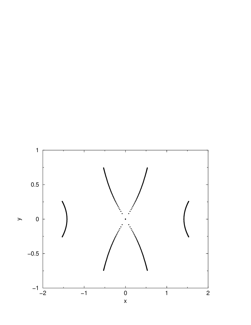
Figure 10: Support of the density of states of the periodic word $\{+++-\}$.

Figure 11: Support of the density of states of the composition of the two words in Figs. 9 and 10.

We see the superposition principle at work.

From this discussion it becomes clear why the spectrum of the matrix $H$ in FZ is so complicated. The sequence $\{r_{1},r_{2},\cdots r_{\infty}\}$ is a book written in the binary alphabet that, in the mathematical limit $N\rightarrow\infty$, contains all possible words, sentences, and paragraphs. In fact, $H$ contains everything ever written or that will be written in the history of the universe, including this particular paper. This familiar mind boggling fact accounts for the complicated looking spectrum first observed in FZ.

It also explains why numerical studies of the spectrum suggest that it is $0-$dimensional. Even for $N$ as large as $1000$ the sequence contains an infinitesimally small subset of the set of all possible words, sentences, and paragraphs.

VII Eigenvalues on the Unit Circle

In the ensemble of all books there are particularly simple books such that $\{r_{1},r_{2},\cdots r_{\infty}\}$ consists of a word $w$ of length $L$ repeated again and again. In this case, we can determine the spectrum explicitly by two different methods.

Let $W$ be the transfer matrix corresponding to $w.$ In other words, $W=\prod\limits_{j=1}^{L}\left(\begin{array}[]{ll}z&-w_{j}\\ 1&0\end{array}\right),$ where the matrix product is ordered. After repeating the word $R$ times, we have

$$\left(\begin{array}[]{l}\Delta_{RL+1}\\ \Delta_{RL}\end{array}\right)=W^{R}\left(\begin{array}[]{l}\Delta_{1}\\ \Delta_{0}\end{array}\right).$$ (31)

Diagonalizing $W=S^{-1}\left(\begin{array}[]{ll}\lambda_{1}(z)&0\\ 0&\lambda_{2}(z)\end{array}\right)S,$ we see immediately that $\Delta_{RL}$ is a linear function of $\lambda_{1}^{R}(z)$ and $\lambda_{2}^{R}(z):$

$$\Delta_{RL}=\alpha\lambda_{1}^{R}+\beta\lambda_{2}^{R}.$$ (32)

We remind the reader that all quantities in (32) are functions of $z.$

The spectrum of $H$ is determined by the zeroes of $\Delta_{RL}(z)$ as $R\rightarrow\infty.$ We note that in this limit the solution of

$$\Delta_{RL}(z)=0$$ (33)

does not depend on knowing the detailed form of $\alpha$ and $\beta.$ Indeed, (33) implies

$$\lambda_{1}=\left(-\frac{\beta}{\alpha}\right)^{\frac{1}{R}}\lambda_{2}$$ (34)

or

$$\lambda_{1}^{2}=\pm\left(-\frac{\beta}{\alpha}\right)^{\frac{1}{R}},$$ (35)

since $\mathrm{\det}\,W=\lambda_{1}\lambda_{2}=\pm 1.$ In the limit $R\rightarrow\infty,$ $(-{\beta}/{\alpha})^{\frac{1}{R}}$ tends towards a ($z-$dependent) complex number of modulus unity. Thus, we conclude that

$$|\lambda(z)|=1,$$ (36)

namely, that the eigenvalues of $W$ lie on the unit circle. This constraint suffices to determine the eigenvalues of $H.$ Plugging (36), that is $\lambda=e^{i\theta},$ into the eigenvalue equation

$$\lambda^{2}-(\mathrm{tr}\,W)\lambda+\mathrm{\det}\,W=0,$$ (37)

we obtain $(\mathrm{tr}\,W)=2\cos\theta$ if $\mathrm{\det}\,W=+1$ and $(\mathrm{tr}\,W)=2i\sin\theta$ if $\mathrm{\det}\,W=-1$, which we can combine into the single equation

$$(\mathrm{tr}\,W)=2(\mathrm{\det}\,W)^{\frac{1}{2}}\cos\theta$$ (38)

after a trivial phase shift.

As $\theta$ ranges from $0$ to $2\pi,$ this traces out the spectrum in the complex plane. As an example, consider the $4-$letter word $\{+++-\}$, in which case (38) reduces to

$$z^{4}-2z^{2}=2i\cos\theta.$$ (39)

This traces out the algebraic curve shown in Fig. 12, which is to be compared to Fig. 10.

Figure 12: Support of the density of states of the word $\{+++-\}$ as given by eq. 39.

Of course, since $H$ is now translation invariant with period $L$, we can apply Bloch’s theorem to determine the spectrum of $H.$ Imposing $\psi_{k+L}=e^{i\varphi}\psi_{k}$ we reduce the eigenvalue problem of $H$ to the eigenvalue problem of the $L$ by $L$ matrix

$$h_{L}=\left(\begin{array}[]{llllll}0&1&0&\cdots&0&r_{L}e^{-i\varphi}\\ r_{1}&0&1&\ddots&0&0\\ 0&r_{2}&0&1&\ddots&\vdots\\ \vdots&\ddots&\ddots&\ddots&\ddots&0\\ 0&0&\ddots&r_{L-2}&0&1\\ e^{i\varphi}&0&\cdots&0&r_{L-1}&0\end{array}\right).$$ (40)

One can verify that with a suitable relation between $\theta$ and $\varphi$ the eigenvalue equation $\mathrm{Det}\,(zI_{L}-h)=0$ becomes identical to (38).

VIII Conclusion and Open Questions

We have seen that the structure of this simple tridiagonal non-Hermitian random matrix possesses an amazing richness. This complexity can be understood if one realizes that the spectrum of the random matrix is the sum of the spectra of all tridiagonal matrices with a periodic subdiagonal obtained by repeating an infinite number of times any finite word of length $L$, weighted by a factor $1/2^{L}$.

The number of lines does not have the cardinal of the continuum. The number of lines is equal to the number of words of any length that can be made with a 2-letter alphabet; this is a countable number.

There are many open questions concerning the fine structure of the spectrum, such as whether the spectrum contains holes in the complex plane (in its domain of definition). We also have not touched upon the question of the nature of the eigenstates. Are they localized or delocalized? Numerical data seems to suggest a localization transition. We hope to address these and other questions in future work.

IX Acknowledgements

One of us (HO) would like to thank M. Bauer, D. Bernard and J.M. Luck for helpful discussions. This work was partially supported by the NSF under grant PHY99-07949 to the ITP.

X Appendix: Cyclic Invariants

As remarked in the text, the coefficients of $Q_{L}(z),$ an even polynomial of degree $2L,$ must be constructed out of the cyclic invariants made of $w_{1},w_{2},\cdots,w_{L}.$ There is presumably a well-developed mathematical theory of cyclic invariants, but what we need we can easily deduce here.

For any $L,$ we have the two obvious cyclic invariants $s=\sum_{j=1}^{L}w_{j}$ and $p=\Pi_{j=1}^{L}w_{j}.$ The number of cyclic invariants grows rapidly with $L.$ Apparently different cyclic invariants can be constructed out of other cyclic invariants, for example, $(\sum_{j=1}^{L}w_{j})^{2}-(\sum_{j=1}^{L}w_{j}^{2})=2\sum_{j\neq i}^{L}w_{j}w_{i}.$

It is easy to work out $Q_{L}(z)$ for low values of $L,$ as follows:

$$Q_{2}(z)=z^{4}-2sz^{2}+d^{2}$$ (41)

with $d\equiv w_{1}-w_{2}$,

$$Q_{3}(z)=(z^{3}-sz)^{2}-4p=z^{6}-2sz^{4}+s^{2}z^{2}-4p,$$ (42)

where we have written $Q_{3}(z)$ in a form which shows that its roots can be found explicitly,

$$Q_{4}(z)=z^{8}-2sz^{6}+(s^{2}+2\kappa)z^{4}-2s\kappa z^{2}+\omega^{2}$$ (43)

with $\kappa\equiv w_{1}w_{3}+w_{2}w_{4}$ and $\omega\equiv w_{1}w_{3}-w_{2}w_{4},$

$$Q_{5}(z)=z^{10}-2sz^{8}+(s^{2}+2\kappa)z^{6}-2s\kappa z^{4}+\kappa^{2}z^{2}-4p,$$ (44)

with $\kappa\equiv w_{1}w_{3}+w_{1}w_{4}+w_{2}w_{4}+w_{2}w_{5}+w_{3}w_{5},$

$$Q_{6}(z) = z^{12}-2sz^{10}+(s^{2}+2\kappa)z^{8}-2(s\kappa+\rho)z^{6}$$ (45)

$$+(\kappa^{2}+2s\rho)z^{4}-2\kappa\rho z^{2}+\delta^{2},$$

where

$$\kappa = w_{1}w_{3}+w_{1}w_{4}+w_{2}w_{4}+w_{1}w_{5}+w_{2}w_{5}+w_{3}w_{5}$$

$$+w_{2}w_{6}+w_{3}w_{6}+w_{4}w_{6}$$

$$\rho = w_{1}w_{3}w_{5}+w_{2}w_{4}w_{6}$$

$$\delta = w_{1}w_{3}w_{5}-w_{2}w_{4}w_{6}$$

and

$$Q_{7}(z) = z^{14}-2sz^{12}+(s^{2}+2\kappa)z^{10}-2(s\kappa+\rho)z^{8}$$ (46)

$$+(\kappa^{2}+2s\rho)z^{6}-2\kappa\rho z^{4}+\rho^{2}z^{2}-4p,$$

with

$$\kappa = w_{1}w_{3}+w_{1}w_{4}+w_{2}w_{4}+w_{1}w_{5}+w_{2}w_{5}+w_{3}w_{5}$$

$$+w_{1}w_{6}+w_{2}w_{6}+w_{3}w_{6}+w_{4}w_{6}+w_{2}w_{7}+w_{3}w_{7}$$

$$+w_{4}w_{7}+w_{5}w_{7}$$

$$\rho = w_{1}w_{3}w_{5}+w_{1}w_{3}w_{6}+w_{1}w_{4}w_{6}+w_{2}w_{4}w_{6}+$$

$$w_{2}w_{4}w_{7}+w_{2}w_{5}w_{7}+w_{3}w_{5}w_{7}.$$

The quantities $d,\kappa,\omega,$ $\kappa,\rho,\delta$ are manifestly cyclic invariants.

References

- (1) J. Feinberg and A. Zee, Phys. Rev. E 59, 6433 (1999).
- (2) N. Hatano and D. R. Nelson, Phys. Rev. Lett. 77, 570 (1996).
- (3) N. Hatano and D. R. Nelson, Phys. Rev. B 56, 8651 (1997).
- (4) J. Feinberg and A. Zee, Nucl. Phys. B 552 599 (1999).
- (5) D. R. Nelson and N. M. Shnerb, Phys. Rev. E 58, 1383 (1998).
- (6) I. Y. Goldsheid and B. A. Khoruzhenko, Phys. Rev. Lett. 80, 2897 (1998).
- (7) P. W. Brouwer, P. G. Silvestrov, and C. W. J. Beenakker, Phys. Rev. B 56, R4333 (1997).
- (8) K. B. Efetov, Phys. Rev. Lett. 79 491 (1997).
- (9) J. Feinberg and A. Zee, Nucl. Phys. B 504 579 (1997).
- (10) E. Brézin and A. Zee, Nucl. Phys. B 509, 599 (1998).
- (11) A. Zee, Physica A 254, 300 (1998).
- (12) N. Hatano, Physica A 254, 317 (1998).
- (13) C. Mudry, P. W. Brouwer, B. I. Halperin, V. Gurarie, and A. Zee, Phys. Rev. B 58, 13539 (1998).
- (14) B. Derrida, J. Lykke Jacobsen, and R. Zeitak, J. Stat. Phys. 98, 31 (2000).
- (15) G.M. Cicuta, M. Contedini, and L. Molinari, J. Stat. Phys. 98, 685 (2000).
- (16) D. Gross and A. Zee, unpublished.
- (17) M. Bauer, D. Bernard, and J.M. Luck, J. Phys. A 34, 2659 (2001).
- (18) C. Sire and P.L. Krapivsky, J. Phys. A 34 9065 (2001).
- (19) F. J. Dyson, Phys. Rev. 92, 1331 (1953).
- (20) H. Schmidt, Phys. Rev. 105, 425 (1957).
- (21) V.I. Oseledec, Trans. Moscow Math. Soc. 19, 197 (1968).
- (22) R. Bruinsma and G. Aeppli, Phys. Rev. Lett. 50, 1494 (1983).
- (23) J.M. Normand, M.L. Mehta, and H. Orland, J. Phys. A 18, 621 (1985).
- (24) J.M. Luck, “Systèmes Désordonnés Unidimensionnels (Paris: Collection Aléa-Saclay, 1992).