The Ferromagnetic Heisenberg XXZ chain in a pinning field

Abstract

We investigate the effect of a magnetic field supported at a single lattice site on the low-energy spectrum of the ferromagnetic Heisenberg XXZ chain. Such fields, caused by impurities, can modify the low-energy spectrum significantly by pinning certain excitations, such as kink and droplet states. We distinguish between different boundary conditions (or sectors), the direction and also the strength of the magnetic field. E.g., with a magnetic field in the $z$-direction applied at the origin and $++$ boundary conditions, there is a critical field strength $B_{c}$ (which depends on the anisotropy of the Hamiltonian and the spin value) with the following properties: for $B<B_{c}$ there is a unique ground state with a gap, at the critical value, $B_{c}$, there are infinitely many (droplet) ground states with gapless excitations, and for $B>B_{c}$ there is again a unique ground state but now belonging to the continuous spectrum. In contrast, any magnetic field with a non-vanishing component in the $xy$-plane yields a unique ground state, which, depending on the boundary conditions, is either an (anti)kink, or an (anti)droplet state. For such fields, i.e., not aligned with the $z$-axis, excitations always have a gap and we obtain a rigorous lower bound for that gap.

I Introduction

The quantum spin-$j$ Heisenberg XXZ chain has been the focus of intensive studies in recent years. The spin 1/2 chain by itself has connections with a surprising variety of interesting mathematical structures, such as quantum groups Pasquier and Saleur (1990), vertex algebras Jimbo and Miwa (1995), and fundamental problems in combinatorics Kuperberg (1996); Batchelor et al. (2001), to name just a few. Of course, the interest in the XXZ model is not limited to mathematics. In 1995, Alcaraz, Salinas, and Wreszinski Alcaraz et al. (1995) and, independently, Gottstein and Werner Gottstein and Werner discovered that, with suitable boundary terms, the ferromagnetic XXZ chain possesses a family of kink ground states which describe a domain wall of finite thickness (these domain walls are exponentially localized, with a width depending on the anisotropy parameter $\Delta$, which diverges as $\Delta\downarrow 1$). Moreover, it was shown in Alcaraz et al. (1995), that similar states exist for the spin $j$ model for arbitrary $j$ and in all dimensions.

From the physical point of view, the discovery of Giant Magnetoresistance and its connection with transport properties in the presense of magnetic domain walls has also spurred renewed interest in the microscopic description of domain walls Dantas et al. (2000); van Gorkom et al. (1999); Jonkers et al. (1999); Koma and Yamanaka ; Koma and Yamanaka (1999, 2000); Mibu et al. (1998); Nakanishi and Nakamura (2000); Tatara and Fukuyama (1997); Wegrowe et al. (2000). Of particular relevance are low-lying excitations associated with them. Koma and Nachtergaele discovered that, although the XXZ model has a gap in its spectrum above the trivial translation invariant ground states, gapless excitations exists associated with diagonal domain walls (11, 111, …) in two or more dimensions Koma and Nachtergaele (1996). The scaling behavior of these excitations was recently determined in Bolina et al. (2000) and Caputo and Martinelli (2001), Caputo and Martinelli (2002).

It is interesting to note that the kink and antikink ground states were discovered by a careful study of the XXZ chain with the special boundary conditions that make the spin 1/2 model $SU_{q}(2)$-symmetric. Although this quantum group symmetry is destroyed for $j>1/2$ or $d>1$, interface ground states exist in general. In one dimension it has been proven rigorously that no other ground states exist, in the sense of local stability, no matter what boundary conditions are considered Matsui (1996); Koma and Nachtergaele (1998). In the last reference it was also proved that the XXX chain does not have domain wall ground states that are stable in the infinite-volume limit.

There is an obvious need for a clear understanding of excitations near magnetic interfaces in order to develop more accurate models of electron scattering at such interfaces. It has been noted, however, that pinning of interfaces by impurities may have to be taken into account as well Jonkers et al. (1999). Here, we study the XXZ chain perturbed at one site by a magnetic field as a caricature model for a pinned domain wall. Admittedly, the one-dimensional nature of the model restricts its direct applicability to experimental situations. We will see however that the low-lying spectrum of this model of pinned interfaces exhibits a number of interesting features that we expect will carry over, mutatis mutandis, to the two- and three-dimensional case.

Let us now define the model precisely and briefly summarize our main results. The spin $j$ XXZ Hamiltonian without boundary terms and with anisotropy parameter $\Delta>1$ is defined on the finite chain labeled by the integers from $a$ to $b$ by

$$H_{0}=-\sum_{x=a}^{b-1}\left[\frac{1}{\Delta}(S^{1}_{x}S^{1}_{x+1}+S^{2}_{x}S^{2}_{x+1})+S^{3}_{x}S^{3}_{x+1}-j^{2}{\bf 1}\right],$$ (1)

where the copies of the spin operators at position $x$, $S_{x}^{1},S_{x}^{2},S_{x}^{3}$ satisfy the usual commutation relations:

$$[S_{x}^{\alpha},S_{x}^{\beta}]=i\,\epsilon^{\alpha\beta\gamma}\,S_{x}^{\gamma}.$$ (2)

The anisotropy $\Delta>1$ has been put in front of the ${\sf XX}$ part so that we can easily take the Ising limit $\Delta\to\infty$. Unless otherwise stated, we set $a=1$. We consider the perturbation of $H_{0}$ obtained by adding a term $\vec{B}\cdot\vec{S}_{y}$, i.e. a magnetic field at the site $y$. As a way to impose boundary conditions, we also add magnetic fields in the $z$-direction at the boundary spins. First, consider boundary fields in the negative $z$-direction at both ends, which we will refer to as ($++$) boundary conditions (b.c.), indicating that they favor the spins at the ends to point in the positive $z$-direction.

If the perturbation at the interior site $y$ has a component orthogonal to the $z$-direction, we find that the ground state is unique and describes a droplet state, i.e., the magnetization is reduced from its maximum possible value in some neighborhood of $y$. Strictly speaking, the magnetization is reduced everywhere in the chain, but by an amount that decays exponentially fast away from $y$.

However, when the field is in the $z$-direction, then there is a critical value $B_{c}$ such that for $B<B_{c}$, the all spin-up state is the ground state. At $B=B_{c}$, there are infinitely many ground states which are droplet states describing domains of negative magnetization of arbitrary size embedded in a environment of positive magnetization. For stronger fields, $B>B_{c}$, the magnetic field selects the all spin-down state as its ground state. This is illustrated in Figure 1.

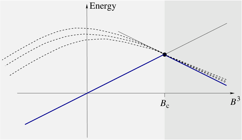
Figure 1: Ground state energy (thick line) in a magnetic field in the $z$-direction and $(++)$ or $(--)$ b.c.. The dotted lines indicate droplet states which describe excitations except at one value of the field strength, $B_{c}$, given in Proposition II.4. Also see Figure 6.

The ground state picture is simpler when we impose ($+-$) b.c., i.e. fields in opposite directions at the boundary spins. For boundary fields of magnitude (3), and without a perturbation in the interior, we then have a set of kink states as the ground state, one for every possible value of the magnetization Alcaraz et al. (1995); Gottstein and Werner . In that case, any non-zero field $\vec{B}$ at an interior site $y$ selects a unique ground state. If $\vec{B}$ is parallel to the $z$-direction the ground state is in the continuous spectrum, and hence there are excitations of arbitrary small energy. If there is a non-vanishing component of $\vec{B}$ in the $xy$-plane, the unique ground state is separated by a gap form the rest of the spectrum. The unique ground state is a kink state centered at a position which we calculate. We also obtain an estimate for the gap.

In Section 2, we define the model and find the set of ground states. Section 3 is devoted to the study of the gap in the spin $1/2$ case. Some less illuminating calculations are presented in three appendices.

II The model and its ground states

The main lesson to be learned from the proof of completeness of the list of ground states of the infinite ferromagnetic XXZ chain (cf. Koma and Nachtergaele (1997)), is that one only needs to study finite chain Hamiltonians with very simple b.c. This remains true if we add a bounded perturbation with finite support to the Hamiltonian, e.g., a magnetic field at one site. These simple b.c. are fields in the $z$-direction with either equal or opposite sign which we will introduce shortly.

The Hamiltonian $H_{0}$, defined in (1), is non-negative, and the two translation invariant all spin-up/down states are the ground states of $H_{0}$. It will be convenient to separate them by adding the equal-sign boundary fields, $jA(S_{1}^{3}+S_{b}^{3})$ with

$$A=A(\Delta)=\sqrt{1-\Delta^{-2}},$$ (3)

and define the droplet and antidroplet Hamiltonian

$$H_{0}^{++} = H_{0}-jA(S^{3}_{1}+S^{3}_{b}-2j{\bf 1}),$$ (4)

$$H_{0}^{--} = H_{0}+jA(S^{3}_{1}+S^{3}_{b}+2j{\bf 1}).$$

For convenience we have normalized the ground state energy to 0. By reflecting all $S^{3}_{x}$ into$-S^{3}_{x}$ the two Hamiltonians, $H^{++}$ and $H^{--}$ are unitarily equivalent and we only study $H_{0}^{++}$.

Additional ground states emerge when we add opposite-sign boundary terms. It turns out that precisely for the fields $\pm jA(S^{3}_{1}-S^{3}_{b})$ one discovers the full set of new ground states. Therefore, we define the kink and antikink Hamiltonian

$$H_{0}^{+-} = H_{0}-jA(S^{3}_{1}-S^{3}_{b}),$$ (5)

$$H_{0}^{-+} = H_{0}+jA(S^{3}_{1}-S^{3}_{b}).$$ (6)

Again, by spin reflection, the kink and anti-kink Hamiltonians are unitarily equivalent. Let us define

$$h_{xx+1}^{+-} = -{\textstyle\frac{1}{\Delta}}(S^{1}_{x}S^{1}_{x+1}+S^{2}_{x}S^{2}_{x+1})-S^{3}_{x}S^{3}_{x+1}+j^{2}{\bf 1}$$ (7)

$$-jA(S^{3}_{x}-S^{3}_{x+1}),$$

and

$$h_{xx+1}^{-+} = -{\textstyle\frac{1}{\Delta}}(S^{1}_{x}S^{1}_{x+1}+S^{2}_{x}S^{2}_{x+1})-S^{3}_{x}S^{3}_{x+1}+j^{2}{\bf 1}$$ (8)

$$+jA(S^{3}_{x}-S^{3}_{x+1}).$$

In terms of these interactions terms we may write

$$H_{0}^{+-}=\sum_{x=1}^{b-1}h_{xx+1}^{+-},$$ (9)

and

$$H_{0}^{-+}=\sum_{x=1}^{b-1}h_{xx+1}^{-+}.$$ (10)

This will be used in Section 3.

It is useful to introduce another parameter, $0<q<1$, such that $q+q^{-1}=2\Delta$. The Hamiltonians defined in (5) and (6) in the spin 1/2 case, commute with a representation of $SU_{q}(2)$. For $j>1/2$, the only obvious conserved quantity is the total $S^{3}$-component, which commutes with all the Hamiltonians defined above.

In the following we first deal with the kink Hamiltonian, $H_{0}^{+-}$. There is a unique ground state for each value (sector) $m$ of $S^{3}$, all of which have the same energy 0. The eigenvalues, $m_{x}$, of $S_{x}^{3}$ are in $\{-j,-j+1,\ldots,j-1,j\}$, such that the total $S^{3}$-component takes the values $m=\sum_{x\in[1,b]}m_{x}$. The eigenvectors of $S^{3}$ are denoted by $|(m_{x})\rangle$, and we have $S_{y}^{3}|(m_{x})\rangle=m_{y}|(m_{x})\rangle$. Further, let

$$w_{m}=\sqrt{2j\choose m+j}.$$

The unique ground states in the respective $S^{3}$-sectors are called kink states which were found by Alcaraz, Salinas and Wreszinski Alcaraz et al. (1995). They are given by

$$\psi_{m}=\sum_{\{m_{x}\}}\prod_{x=1}^{b}q^{-x(j-m_{x})}w_{m_{x}}|(m_{x})\rangle,$$ (11)

As the $\psi_{m}$ are not normalized, we also define $\phi_{m}=\psi_{m}/\|\psi_{m}\|$. The sum over $\{m_{x}\}$ is restricted to combinations such that $\sum m_{x}=m$. If $m=\pm jb$ is maximal/minimal, then the state $\phi_{m}$ is the all spin-up/down state, i.e. the magnetization profile in the $z$-direction, $\langle\phi_{m}|S_{x}^{3}|\phi_{m}\rangle=\pm j$. Both from a physical and mathematical point of view, the infinite chain limit is the most interesting case. Clearly, more care has to be taken when using an infinite volume Hamiltonian. The natural tool is the GNS representation. In our case here, there are four (unitarily) inequivalent representations on Hilbert spaces, which are also called sectors. These are the (anti)kink sectors containing the infinite volume (anti)kink ground states, and the (anti)droplet sectors with the all spin (down)up ground state. As mentioned above, for the infinite volume limit it is sufficient to study the effect of the perturbation for the finite chain Hamiltonians, $H_{0}^{++}$ and $H_{0}^{+-}$. For more details, we refer to Koma and Nachtergaele (1997).

For our purposes it will be very convenient to define the states

$$\psi(z)=C\sum_{|m|\leq jb}z^{jb-m}\psi_{m}.$$ (12)

where $C$ is a normalization constant. They are product states, i.e.

$$\psi(z)=\bigotimes_{x=1}^{b}\chi_{x}(z),$$ (13)

with

$$\chi_{x}(z)=(1+|z|^{2}q^{-2x})^{-j}\sum_{m_{x}=-j}^{j}(zq^{-x})^{j-m_{x}}w_{m_{x}}|(m_{x})\rangle.$$ (14)

The same construction can be carried through for the antikink Hamiltonian. We denote the corresponding states for the antikink Hamiltonian by $\tilde{\psi}(z)$. If we let

$$\tilde{\chi}_{x}(z)$$

$$= (1+|z|^{2}q^{-2x})^{-j}\sum_{m_{x}=-j}^{j}(zq^{-x})^{j-m_{x}}w_{m_{x}}|(-m_{x})\rangle,$$

then $\tilde{\psi}(z)=\bigotimes_{x=1}^{b}\tilde{\chi}_{x}(z)$ are ground states of $H^{-+}$.

Now, let $\vec{B}=(B_{1},B_{2},B_{3})$ be a magnetic field vector with (real) parameters, and $V=\vec{B}\cdot\vec{S}=B_{1}S^{1}+B_{2}S^{2}+B_{3}S^{3}$. Then the eigenvalues of $V$ are $\|\vec{B}\|\cdot m$ with $m=-j,-j+1,\ldots,j$. Define

$$H^{+-}(\vec{B}) = H_{0}^{+-}+\vec{B}\cdot\vec{S}_{y},$$ (16)

$$H^{++}(\vec{B}) = H_{0}^{++}+\vec{B}\cdot\vec{S}_{y}.$$ (17)

In the study of the spectrum of $H^{+-}(\vec{B})$ and $H^{-+}(\vec{B})$, it is important to distinguish two cases: $B_{1}^{2}+B_{2}^{2}>0$ and $B_{1}^{2}+B_{2}^{2}=0$. The ground state in these two cases is described in Propositions II.1 and II.3, and the Remarks II.2.

PROPOSITION II.1 (Kink sector, $B_{1}^{2}+B_{2}^{2}>0$).

Let $1\leq y\leq b$. Then, the ground state of $H^{+-}(\vec{B})$ is the state $\psi(z)$ of eq (13) with $z=-\frac{\|\vec{B}\|+B_{3}}{B_{1}-iB_{2}}\,q^{y}$. Its energy is $-j\|\vec{B}\|$.

The proof is a combination of previously known results and a straightforward calculation. See Appendix A.

REMARKS II.2.

1. The ground state of $H^{-+}(\vec{B})$ is the state $\tilde{\psi}(\tilde{z})$ of equation (II) with $\tilde{z}=-\frac{\|\vec{B}\|-B_{3}}{B_{1}+iB_{2}}\,q^{y}$. This follows by a rotation by the angle $\pi$ with respect to the $x$-axis.

2. For simplicity, let us assume that $B_{1}^{2}+B_{2}^{2}=1$. If $B_{3}=0$, then the ground state, $\psi(z=-(B_{1}+iB_{2})\,q^{y})$, is a kink state (exponentially) localized at the magnetic field at $y$; among the spanning set of ground states $\psi(z)$, the perturbation picks the one which is most localized at $y$. If $B_{3}\neq 0$, the extra term $B_{3}S_{y}^{3}$ has the effect of shifting the kink from $y$ by the distance $|\log_{q}{(\sqrt{1+B_{3}^{2}}+B_{3})}|$ to the left if $B_{3}>0$, and to the right (by the same distance) if $B_{3}<0$.

3. The proof also shows that the state $\psi(z)$ with $z=+\frac{\|\vec{B}\|+B_{3}}{B_{1}-iB_{2}}\,q^{y}$ is an eigenstate of $H^{+-}(\vec{B})$ with energy $+j\|\vec{B}\|$. We see this (it is obviously linear if the field is in the $x$ or $y$ direction only, see Figure 2) branch ascending from $|B_{3}|/2$ in Figure 2-3. In Figure 4 it has too high an energy to be among the plotted lowest eigenvalues.

4. Of special interest is the second-lowest eigenvalue, in particular, whether there is a gap uniformly in the number of sites, $b$, and how it depends on $\vec{B}$ and the anisotropy $\Delta$. This will be treated in Section 3. We can extend a method Nachtergaele (1996) which was first applied to prove a gap for $H^{+-}_{0}$.

5. We discuss now qualitatively the low energy spectrum, and assume for simplicity that $j=1/2$ and $B_{2}=0$. It was proven in Koma and Nachtergaele (1997) that the gap above the $b+1$ ground states of the unperturbed Hamiltonian, $H_{0}^{+-}$, is equal to $1-\cos{(\pi/b)}\Delta^{-1}$, which tends to $1-\Delta^{-1}$ in the infinite chain limit.

   If $B_{3}=0$, then there are $b$ eigenvalues (recall, $b$ is the length of the chain) of $H^{+-}(B,0,0)$ descending from 0. This can be seen as follows. We introduce the function $N(B)=\chi_{(-\infty,0]}\left(H^{+-}(B,0,0)-\frac{1}{2}B{\bf 1}\right)$ counting the number of non-positive eigenvalues; here $\chi_{(-\infty,0]}$ is the characteristic function of $(-\infty,0]$. $N(B)$ is monotonically increasing, and equal to $b+1$ for $|B|<1-\Delta^{-1}+{\cal O}(b^{-1})$; this is guaranteed by the gap above the ground states. In item 6 below we calculate the lowest energy state, $\psi_{e}$, descending from $1-\Delta^{-1}$ at $B=0$ with energy equal to $1-\Delta^{-1}-\frac{1}{2}|B|$ (up to ${\cal O}(b^{-1})$). This state is ‘parallel’ to the ground state energy and intersects with the state in item 2 at $|B|=1-\cos{(\pi/b)}\Delta^{-1}$, see Figure 2.

   We can say more about the average of these lowest $b+1$ eigenvalues by recalling the Min-max Principle, namely that their average is a concave function in $B$. By symmetry ($B\to-B$) its (left and right) derivative is always negative and less than $1/2$. Since the average is 0 at $B=0$ it continues to be negative. In the infinite volume limit there is an infinite number of ground states of $H_{0}^{+-}$, and eigenvalues for $H^{+-}(B,0,0)$ have to accumulate at some value between $-\frac{1}{2}|B|$ and $1-\Delta^{-1}-\frac{1}{2}|B|$, see Figure 2, and in case $B_{3}\not=0$, see Figures 3-4.

6. If $B_{3}\not=0$, then there appear to be $b-y+1$ eigenvalues descending from $-|B_{3}|/2$; $b-y+1$ is the number of kinks to the left of $y$, see Figure 3. The next eigenvalues depend on $B_{3}$. If $|B_{3}|<1-\Delta^{-1}$, then the next lowest $y$ eigenvalues descend from $-|B_{3}|/2$. If $|B_{3}|>1-\Delta^{-1}$, then the state $\psi_{e}$ appears to be the next lowest in energy, see Figure 4.

7. We can calculate the state mentioned in the previous two items. Let $\psi_{e}=\sum_{x=1}^{b}a_{x}S_{x}^{-}|\!\!\uparrow\rangle$ be the first excited state of $H_{0}^{+-}$ in the one-overturned spin-sector. The coefficients $a_{x}$ are a solution to the discrete Laplace equation (see Koma and Nachtergaele (1998), or cf. Appendix C by setting $B=0$). The energy of $\psi_{e}$ is equal to the gap $1-\Delta^{-1}+{\cal O}(b^{-1})$. Now, define

   $$\psi_{e}(z)=\sum_{n=0}^{b}z^{n}(S_{q}^{-})^{n}\psi_{e}=\sum_{x=1}^{b}a_{x}S_{x}^{-}\psi(z).$$

   By choosing $z$ as in Proposition II.1, we obtain the equation

   $$H^{+-}(\vec{B})\psi_{e}(z)=\left(1-\Delta^{-1}-{\textstyle\frac{1}{2}}\|\vec{B}\|\right)\psi_{e}(z)+{\cal O}\left(b^{-1}\right).$$

   In Figure 2, this is the straight line parallel to the ground state energy.

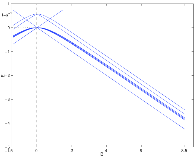
Figure 2: Energy of the lowest 16 eigenvalues for the spin $1/2$ kink Hamiltonian for the field $(B,0,0)$ on a chain of 13 sites and $\Delta=2.25$. Notice the ground state energy (straight line downwards from 0), the gap to the 2nd eigenvalue, the energy $\frac{1}{2}|B|$, and the energy $1-\Delta^{-1}-|B|/2$ of $\psi_{e}$.

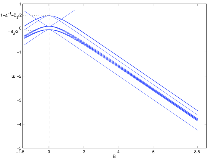
Figure 3: Energy of the lowest 16 eigenvalues for the spin $1/2$ kink Hamiltonian for the field $(B,0,A/6)$ on a chain of 13 sites and $\Delta=2.25$; the $z$-component, $B_{3}=A/6=\sqrt{1-\Delta^{-1}}/6$ is chosen small compared to the gap $1-\Delta^{-1}$ of $H_{0}^{+-}$. Notice the ground state energy, the gap above it, and the branches descending from $\pm B_{3}/2$, and $1-\Delta^{-1}-B_{3}/2$.

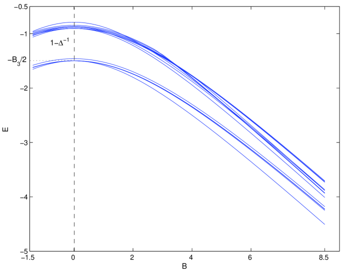
Figure 4: Energy of the lowest 20 eigenvalues for the spin $1/2$ kink Hamiltonian with the field $(B,0,3)$ on a chain of 13 sites and $\Delta=2.25$; the field in the $z$-direction is chosen large compared to $1-\Delta^{-1}$. Notice that the branches stemming from $B_{3}/2$ are too high in energy to be plotted here. We see the ground state energy, the gap above it, and the energy of $\psi_{e}$ descending from $1-\Delta^{-1}-B_{3}/2$. In between there are $b-y+1=6$ states bending downwards from $-B_{3}/2=-1.5$.

Next, we consider the kink sector and magnetic fields of the form $B_{1}=B_{2}=0,B=B_{3}\not=0$. Let $B>0$. Then, as $b$, the size of the system increases, the ground state tends to the all spin-down state, $|\!\downarrow\rangle$. This vector is no longer in the infinite volume kink-sector very much as $e^{ikx}$ is not a genuine (i.e., normalizable) eigenvector of the Laplacian on the real line. In other words, $|\!\downarrow\rangle$ is part of the continuous spectrum. So let us consider the orthogonal sequence of kink states, $\psi_{n}$; $n$, as usual, is the total $z$-component. Then, the sequence $\langle\psi_{n},H^{+-}(0,0,B),\psi_{n}\rangle$ converges to $-jB$ as $n\to-\infty$. Since the spectrum is closed and $-jB$ is the least possible eigenvalue it has to be the ground state energy. Therefore, in the infinite chain limit, $-jB$ is contained in the continuous spectrum, and is hence non-isolated. We conjecture that there is no other continuous spectrum close to $-j|B|$, and thus $-j|B|$ is purely an accumulation point of eigenvectors. We do not give a proof of this here. Similarily, if $B<0$, then the bottom of the spectrum is $jB$ and there is no gap above the ground state, which is obviously the all spin-up state. We illustrate the low energy spectrum in Figure 5.

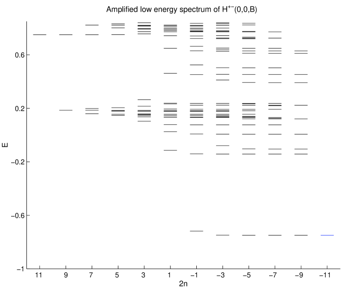
Figure 5: Low energy spectrum in the spin $1/2$ kink sector for the field $(0,0,1.5)$ on a chain of 11 sites with $\Delta=2.25$. The high energy spectrum is similar to Fig. 7 and will not be reprinted. $n$ is the total $z$-component.

Let us collect our results in the following proposition:

PROPOSITION II.3 (Kink sector, $B_{1}^{2}+B_{2}^{2}=0$).

The bottom of the spectrum of $H^{+-}(0,0,B)$ is equal to $-j|B|$, which is part of the continuous spectrum. Excitations above the ground state are gapless.

Now we consider the Hamiltonian $H^{++}(\vec{B})$. It is useful to decompose this as a sum of a kink and anti-kink Hamiltonian ($b\geq 3$):

$$H^{++}_{[1,b]}+2jA\left(-j{\bf 1}+S_{y}^{3}\right)=H^{+-}_{[1,y]}+H^{-+}_{[y,b]},$$

and thus

$$H_{[1,b]}^{++}(\vec{B})-2j^{2}A{\bf 1} = H^{+-}_{[1,y]}({\textstyle\frac{B_{1}}{2}},{\textstyle\frac{B_{2}}{2}},{\textstyle\frac{B_{3}}{2}}-jA)$$ (18)

$$+H^{-+}_{[y,b]}({\textstyle\frac{B_{1}}{2}},{\textstyle\frac{B_{2}}{2}},{\textstyle\frac{B_{3}}{2}}-jA).$$

We start with the case $B_{1}^{2}+B_{2}^{2}>0$. As in the kink sector we will find a unique ground state. Let

$$z=-\frac{\|(B_{1},B_{2},B_{3}-2jA)\|+B_{3}-2jA}{B_{1}-iB_{2}}q^{y},$$

then according to Proposition II.1, $\psi_{[1,y]}(z)$ is the unique ground state of $H^{+-}_{[1,y]}(B_{1}/2,B_{2}/2,B_{2}/2-jA)$, while the anti-kink state $\tilde{\psi}_{[y,b]}(\tilde{z})$ is the corresponding ground state of $H^{-+}_{[y,b]}(B_{1}/2,B_{2}/2,B_{3}/2-jA)$. They are both product states which happen to satisfy $\chi_{y}(z)=(-1)^{2j}\tilde{\chi}_{y}(\tilde{z})$, because

$${\textstyle\frac{1}{2}}(B_{1}S_{y}^{1}+B_{2}S_{y}^{2}+(B_{3}-2jA)S_{y}^{3})\chi^{\sharp}(z^{\sharp})$$

$$= -{\textstyle\frac{j}{2}}\|(B_{1},B_{2},B_{3}-2jA)\|\,\chi^{\sharp}(z^{\sharp}),$$

where $\chi^{\sharp}(z^{\sharp})$ stands for either $\chi_{y}(z)$ or $\tilde{\chi}_{y}(\tilde{z})$. Thus

$$\psi(\vec{B})=\bigotimes_{x=1}^{y}\chi_{x}(z)\otimes\bigotimes_{x=y+1}^{b}\tilde{\chi}_{x}(\tilde{z})$$

is the unique ground state of $H^{++}_{0}(\vec{B})$ with energy $-j\|(B_{1},B_{2},B_{3}-2jA)\|+2j^{2}A$.

Similar to the kink-sector, the vector

$$\bigotimes_{x=1}^{y}\chi_{x}(-z)\otimes\bigotimes_{x=y+1}^{b}\tilde{\chi}_{x}(-\tilde{z})$$

is another eigenstate with energy ${j}\|(B_{1},B_{2},B_{3}-2jA)\|+2j^{2}A$.

Finally, we come to the case $B_{1}=B_{2}=0,B=B_{3}$. When $B=0$, it was proven in Nachtergaele and Starr (2001) that for spin $1/2$, and in the infinite volume limit $1-\Delta^{-1}$ is the gap above the ground state. It can also be shown that there exists a gap, $\delta$, for higher spins although no precise estimates are known. This implies that uniformly in the size of the lattice, that the all spin-up vector is the unique ground state for $B<B_{c}=\delta/(2j)$, where $\delta$ is the (strictly positive) gap of $H^{++}_{0}$. As we mentioned in the Introduction, the value $B=A/(2j)$ is very particular and interesting. It has been analyzed Starr (2001) in the context of droplet states for spin $1/2$ but again the method extends to general $j$. In fact, the set of ground states is infinitely degenerate (in the infinite volume) and consists of pairs of symmetric kink-antikink states (i.e. droplets), all of which have the same energy $jA$. The magnetization profile in the $z$-direction is symmetric with respect to the center of the field at $y$. Excitations are gapless because large droplets which are antisymmetric with respect to $y$ come arbitrarily close in energy to $jA$.

Since the ground state energy is concave, and since for $B=0$ and $B=A/2j$, the all spin-up vector is a ground state, we conclude that for all $B<A/(2j)$, the all spin-up vector is the unique ground state. Numerical experiments for spin $1/2$ indicate that in the region $B<A$ the eigenvalues are ordered by their total $S^{3}$-value such that the second-lowest eigenstate is in the sector with one overturned spin, and has energy ${\cal E}_{-}(B)=1-\sqrt{\Delta^{-2}+B^{2}}+\frac{1}{2}|B|$, see (51); its (infinite volume) derivation is given in Appendix C. The third-lowest eigenvector is in the sector with two overturned spins, and so on. The lowest eigenvalues with respect to the total $S^{3}$-component accumulate at the line $A-B/2$. They all meet at the critical value $A$, where the ground state becomes infinitely degenerate. Assuming that this ordering holds true, we conjecture that the gap for spin $1/2$ and $B\leq A$ equals $1-\sqrt{\Delta^{-2}+B^{2}}+\frac{1}{2}(|B|-B)$, which converges to $1-\frac{1}{2\Delta}$ for large $-B$, and vanishes at $B=A$.

For $B>A/(2j)$, the all spin-down state is the unique ground state with energy $A/(2j)-jB$, which is part of the continuous spectrum; in fact, $A/(2j)-jB$ is purely an accumulation point of eigenvectors. It seems that for $B>A/2j$ the eigenvalues are also ordered according to their total $z$-component, $n$, but this time in the opposite way. I.e. lower $n$ means lower energy, and clearly the lowest is the all spin-down state. Similar to the kink sector, we will not prove here that the rest of the continuous spectrum is separated from the ground state.

The situation is illustrated in Fig. 6-8 for $j=1/2$, cf. also Figure 1. Let us summarize our results in the following proposition:

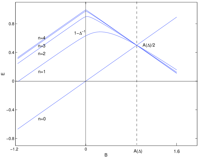
Figure 6: The five lowest eigenvalues in the spin $1/2$ droplet sector for a chain of 13 sites with magnetic field $(0,0,B)$ and $\Delta=2.25$. The eigenvalues are numbered by $n$, the number of overturned spins; e.g. $n=0$ means the all spin-up state.

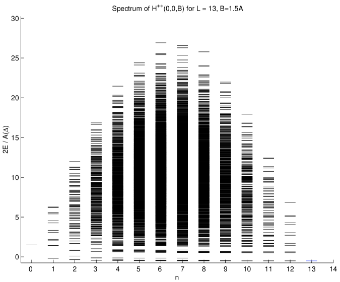
Figure 7: Here, we plot the full spectrum of the spin 1/2 droplet Hamiltonian $H^{++}(0,0,1.5A)$ for 13 sites, and $\Delta=2.25$. The index $n$ is the number of overturned spins. The ground state is the all spin-down state, i.e. $n=13$.

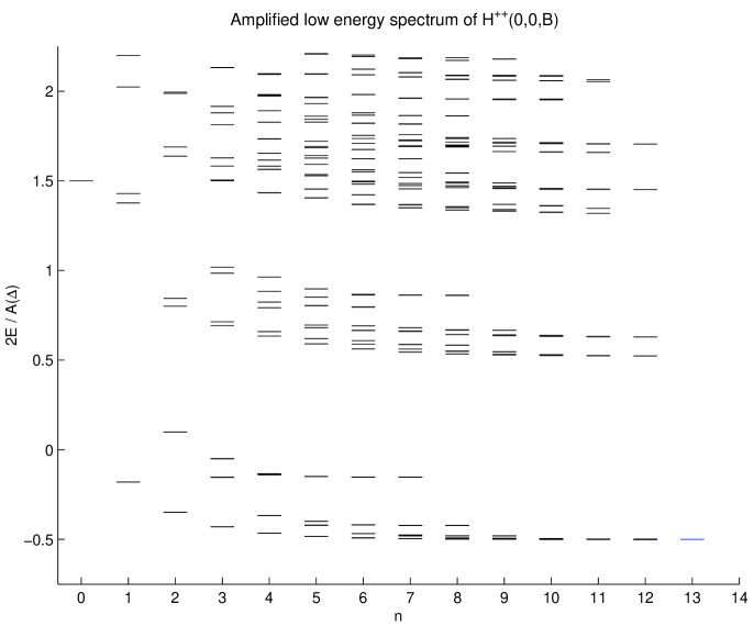
Figure 8: Here, we amplify the low energy spectrum for the same Hamiltonian as in Figure 7. At $n=13$ we have indicated the ground state. Clearly, one sees monotonicity of energy vs $n$.

PROPOSITION II.4 (Droplet sector).

The ground state of the droplet Hamiltonian, $H^{++}(\vec{B})$, on a chain of length $b\geq 3$ depends on the magnetic field $\vec{B}$ in the following way:

1. If $B_{1}^{2}+B_{2}^{2}>0$, then the ground state is unique. The ground state energy is $-{j}\|(B_{1},B_{2},B_{3}-2jA)\|+2j^{2}A$.

2. If $B_{1}=B_{2}=0,B=B_{3}$, and $B_{c}=A/(2j)$, then for $B<B_{c}$ the unique ground state of $H^{++}(0,0,B)$ is the all spin-up vector with energy $jB$. For $B=B_{c}$ the ground states are droplet states which are (in the thermodynamic limit) infinitely degenerate with energy $jA$. In infinite volume, excitations above these ground states are gapless. For $B>B_{c}$, the all spin-down state is the unique ground state, which is an accumulation point of eigenvectors. Hence, excitations are gapless.

III Estimate for the spectral gap in the case $j=1/2$

Here we prove a uniform lower bound on the difference between the ground state energy and the energy of the first excited state for the spin $1/2$ Hamiltonians $H^{+-}_{[1,b]}(\vec{B})$ and $H^{++}_{[1,b]}(\vec{B})$ on a finite chain $[1,b]$ with the impurity field at $y$.

Before we prove these gap inequalities we introduce the methods which were invented in Nachtergaele (1996) and Nachtergaele . Let ${\cal C}_{i},i=0,\ldots,N$ be a sequence of connected intervals with $\bigcup_{i=0}^{N}{\cal C}_{i}=[1,b]$, and such that two intervals have at most one lattice point in common. Let $h_{{\cal C}_{i}}\geq 0$ be some (local) Hamiltonians acting on $\mathbb{C}^{2|{\cal C}_{i}|}$, and define

$$H_{[1,b]}=\sum_{i=0}^{N}h_{{\cal C}_{i}}.$$ (19)

$H_{[1,b]}$ acts on ${\cal H}_{b}=\bigotimes_{i=1}^{b}\mathbb{C}^{2}$. We assume that $\ker{H_{[1,b]}}\not=\{0\}$. Let $\gamma_{i}$ denote the gap of $h_{{\cal C}_{i}}$, i.e. the smallest non-zero eigenvalue of $h_{{\cal C}_{i}}$. It is clear that

$$\ker H_{[1,b]}=\bigcap_{i=0}^{N}\ker h_{{\cal C}_{i}}.$$ (20)

Let $\Lambda\subset[1,b]$, then we define $G_{\Lambda}$ to be the orthogonal projection onto the

$$\ker\sum_{i:{\cal C}_{i}\subset\Lambda}h_{{\cal C}_{i}}.$$ (21)

We use the convention that if ${\cal C}_{i}\not\subset\Lambda$ for any $i$, then we set $G_{\Lambda}=\bf 1$. From these definitions we derive the following properties:

1. $G_{\Lambda}G_{\Lambda^{\prime}}=G_{\Lambda^{\prime}}G_{\Lambda}=G_{\Lambda^{\prime}}$ if $\Lambda\subset\Lambda^{\prime}$.

2. $G_{\Lambda}G_{\Lambda^{\prime}}=G_{\Lambda^{\prime}}G_{\Lambda}$ if $\Lambda\cap\Lambda^{\prime}=\emptyset$.

3. $h_{{\cal C}_{i}}\geq\gamma_{i}({\bf 1}-G_{{\cal C}_{i}})$.

Next we define the intervals $\Lambda_{i}=\bigcup_{j\leq i}{\cal C}_{j}$, and operators $E_{i},i\geq 0$, on ${\cal H}_{b}$ by

$$E_{i}=\left\{\begin{array}[]{lcl}{\bf 1}-G_{\Lambda_{0}}&\mbox{for}&i=0\\ G_{\Lambda_{i}}-G_{\Lambda_{i+1}}&\mbox{for}&1\leq i<N\\ G_{[1,b]}&\mbox{for}&i=N\end{array}\right..$$ (22)

These operators are mutually commuting projections adding up to ${\bf 1}$, i.e.

$$E_{i}^{*}=E_{i},\quad E_{i}E_{j}=\delta_{ij}E_{i},\quad\sum_{i=0}^{N}E_{i}={\bf 1}.$$ (23)

The key assumption in order to deduce a gap for $H_{[1,b]}$ from the gaps of $h_{{\cal C}_{i}}$ is the following assumption:

ASSUMPTION III.1.

There exists a positive constant $\epsilon$ such that $0\leq\epsilon<1/\sqrt{2}$ and

$$E_{i}G_{{\cal C}_{i+1}}E_{i}\leq\epsilon^{2}E_{i},\quad 0\leq i\leq N-1,$$ (24)

or equivalently,

$$\|G_{{\cal C}_{i+1}}E_{i}\|\leq\epsilon,\quad 0\leq i\leq N-1.$$ (25)

Further, we assume that the gaps, $\gamma_{i}$, for the local Hamiltonians are bounded from below, i.e. $\gamma_{i}\geq\gamma>0$.

The conditions (24) and (25) are equivalent due to $G_{{\cal C}_{i+1}}E_{i}=G_{{\cal C}_{i+1}}G_{\Lambda_{i}}$ $-G_{\Lambda_{i+1}}$.

Now we are ready to state the main theorem which we apply in all three case below.

THEOREM III.2 (Nachtergaele Nachtergaele (1996)).

With the above definitions and under the assumptions in (25) let $\psi$ be orthogonal to the ground states of $H_{[1,b]}$. Then

$$(\psi,H_{[1,b]}\psi)\geq\gamma(1-\sqrt{2}\epsilon)^{2}\|\psi\|^{2}.$$ (26)

I.e. the gap in the spectrum of $H_{[1,b]}$ above 0 is at least $\gamma(1-\sqrt{2}\epsilon)^{2}$.

Proof.

Let $\psi$ be orthogonal to the ground state, i.e. $G_{[1,b]}\psi=0$. Then, $\|\psi\|^{2}=\sum_{0\leq n<N}\|E_{n}\psi\|^{2}$.

We estimate $\|E_{n}\psi\|^{2}$ in terms of $(\psi,H_{{\cal C}_{n}}(\vec{B})\psi)$ as follows. First notice, that for $m\leq n-2$, or $m\geq n+1$, $E_{m}G_{{\cal C}_{n}}=G_{{\cal C}_{n}}E_{m}$. Now we insert $G_{{\cal C}_{n}}$ and the resolution of identity, $\{E_{n}\}$, and we get

$$\|E_{n}\psi\|^{2}$$ (27)

$$= (\psi,({\bf 1}-G_{{\cal C}_{n}})E_{n}\psi)+(\psi,\sum_{0\leq m<N}E_{m}G_{{\cal C}_{n}}E_{n}\psi)$$

$$= (\psi,({\bf 1}-G_{{\cal C}_{n}})E_{n}\psi)+((E_{n-1}+E_{n})\psi,G_{{\cal C}_{n}}E_{n}\psi).\hskip 19.91684pt$$

Let $c_{1},c_{2}>0$, then

$$\|E_{n}\psi\|^{2}$$

$$\leq \frac{1}{2c_{1}}(\psi,({\bf 1}-G_{{\cal C}_{n}})\psi)+\frac{c_{1}}{2}(\psi,E_{n}\psi)$$

$$+\frac{1}{2c_{2}}(\psi,E_{n}G_{{\cal C}_{n}}E_{n}\psi)+\frac{c_{2}}{2}(\psi,(E_{n-1}+E_{n})^{2}\psi),$$

where we used the inequality

$$|(\phi_{1},\phi_{2})|\leq\frac{1}{2c}\|\phi_{1}\|^{2}+\frac{c}{2}\|\phi_{2}\|^{2}$$

in both terms of (27). Let $\gamma=\min{\{\gamma_{{\cal C}_{i}}\}}$ be the minimum of the gaps of the Hamiltonians $h_{{\cal C}_{i}}$.

The first term on the rhs of (III) is less than $\frac{1}{2c_{1}\gamma}(\psi,h_{{\cal C}_{n}}\psi)$. Now, assuming the key estimate, $\|G_{{\cal C}_{n}}E_{n}\|<\epsilon$, we see that

$$\left(2-c_{1}-\frac{\epsilon^{2}}{c_{2}}\right)\|E_{n}\psi\|^{2}-c_{2}\|(E_{n-1}+E_{n})\psi\|^{2}$$

$$\leq \frac{1}{c_{1}\gamma}(\psi,h_{{\cal C}_{n}}\psi).\hskip 113.81102pt$$

We sum over $n$ using $\|\psi\|^{2}=\sum_{0\leq n<N}\|E_{n}\psi\|^{2}$ from above and get

$$\left(2-c_{1}-\frac{\epsilon^{2}}{c_{2}}-2c_{2}\right)\|\psi\|^{2}-c_{2}\|\psi\|^{2}\leq\frac{1}{c_{1}\gamma}(\psi,H_{[1,b]}\psi).$$

Finally, we optimize the constants $c_{1},c_{2}$ yielding $c_{1}=1-\epsilon\sqrt{2},c_{2}=\epsilon/\sqrt{2}$. This proves the gap inequality. ∎

In all the upcoming proofs on the various gaps we use the same definition of subsets ${\cal C}_{n},\Lambda_{n}$ of $[1,b]$ and projections $G_{n},E_{n}$. As usual $y\in[1,b]$ denotes the spot of the magnetic field. Let $n_{l},n_{r}$ be some non-negative integers such that $n_{r}+n_{l}\geq 1$, and assume that $n_{r}>0$; the choice of $n_{l},n_{r}$ in general will depend on $\Delta$ and $\vec{B}$. The idea behind the definition of ${\cal C}_{n}$ is that we cover the chain $[1,b]$ by adding points to an initially chosen interval ${\cal C}_{0}=[y-n_{l},y+n_{r}]$ in an alternating manner. First we add a point to the right of ${\cal C}_{0}$, then to the left until we reach the point 1. Then we add points only to the right of ${\cal C}_{2(y-n_{l}-1)}$ until we finish at $b$. More precisely, we define the sets $C_{n}$ in the following way:

DEFINITION III.3.

Let ${\cal C}_{0}=[y-n_{l},y+n_{r}]$, where we may assume that $y-n_{l}-1\leq b-y-n_{r}$ such that ${\cal C}_{0}\subset[1,b]$. The intervals for $n>0$ are then ${\cal C}_{1}=[y+n_{r},y+n_{r}+1],{\cal C}_{2}=[y-n_{l}-1,y-n_{l}],\ldots,{\cal C}_{2(y-n_{l}-1)}=[1,2],{\cal C}_{2(y-n_{l})-1}=[2y+n_{r}-n_{l}-1,2y+n_{r}-n_{l}],\ldots,{\cal C}_{b-(n_{l}+n_{r})-1}=[b-1,b]$.

We start with the kink case.

PROPOSITION III.4 (Kink sector, $B_{1}^{2}+B_{2}^{2}>0$).

Let $\psi$ be orthogonal to the ground state of the kink Hamiltonian, $H^{+-}_{[1,b]}(\vec{B})$, on a chain of length $b$. Then, there exists a strictly positive function $g^{+-}(\vec{B},\Delta)$ and a function $0\leq\epsilon(\vec{B},\Delta)<1/\sqrt{2}$, which are both independent of $b$, such that the following gap inequality is satisfied

$$(\psi,H^{+-}_{[1,b]}(\vec{B})\psi)\geq g^{+-}(\vec{B},\Delta)(1-\sqrt{2}\epsilon(\vec{B},\Delta))^{2}\|\psi\|^{2}.\hskip 19.91684pt$$ (29)

Proof.

First we shift the ground state energy to be 0, and define the new Hamiltonian

$$H_{[1,b]}(\vec{B})=H^{+-}_{[1,b]}(\vec{B})-{\textstyle\frac{\|\vec{B}\|}{2}}{\bf 1}.$$

With the set-up from Definition (III.3) we can write the Hamiltonian, $H_{[1,b]}(\vec{B})$, in the following form:

$$H_{[1,b]}(\vec{B}) = \sum_{i=0}^{b-(n_{l}+n_{r})-1}h_{{\cal C}_{i}}$$

using

$$h_{{\cal C}_{i}} = \left\{\begin{array}[]{lcr}H_{{\cal C}_{0}}(\vec{B})&\mbox{ for }&i=0\\ h_{xx+1}^{+-}&\mbox{ for }&i>0\end{array},\right.$$

where ${\cal C}_{i}=[x,x+1]$ for some $1\leq x<y-n_{l}$ or $y+n_{r}\leq x<b$, and with $h_{xx+1}^{+-}$ from (7).

We can express the gap conditions as

1. $H_{\Lambda_{0}}(\vec{B})\geq g_{\Lambda_{0}}^{+-}(\vec{B},\Delta)({\bf 1}-G_{0})$, where $g_{\Lambda_{0}}^{+-}(\vec{B},\Delta)$ is the gap for the finite chain Hamiltonian, $H^{+-}_{\Lambda_{0}}(\vec{B})$.

2. $h_{xx+1}^{+-}={\bf 1}-G_{[xx+1]}$ for $1\leq x<y-n_{l}$ and $y+n_{r}\leq x<b$.

Let $\gamma=\min{\{g_{\Lambda_{0}}^{+-}(\vec{B},\Delta),1\}}$ which is strictly positive. Finally, we need to verify the second condition in Assumption III.1, and define

$$C_{n}:=\sup_{0\not=\psi\in{\cal H}_{\Lambda_{n+1}}:E_{n}\psi=\psi}\frac{\|G_{{\cal C}_{n}}\psi\|}{\|\psi\|}.$$ (31)

So let $\psi$ satisfy

$$G_{n}\psi=\psi\quad\mbox{and}\quad G_{n+1}\psi=0.$$ (32)

First, let $n=2m,0\leq m\leq y-n_{l}-1$; the case $n\geq 2(y-n_{l})$ is similar, and the case of odd $1\leq n<2(y-n_{l})$ will be considered later.

Let $\psi$ be a ground state of $\Lambda_{n}$, i.e. $G_{n}\psi=\psi$ such that $G_{n+1}\psi=0$. Then with the definition from (14)

$$\psi=\bigotimes_{i={y-n_{l}-m}}^{y+n_{r}+m}\chi_{i}(z)\otimes\chi^{\perp}_{y-n_{r}+m+1}(z),$$

where $\chi^{\perp}_{x}(z)$ is perpendicular to $\chi_{x}(z)$. Let us make some definitions and call $f:=-\frac{\|\vec{B}\|+B_{3}}{B_{1}-iB_{2}}$, $\chi:=\chi_{y+n_{r}+m}(z)=|\!\!\uparrow\rangle+fq^{-n_{r}-m}|\!\!\downarrow\rangle$, $\chi^{\perp}:=\chi_{y+n_{r}+m}(z)=fq^{-n_{r}-m-1}$ $|\!\!\uparrow\rangle-|\!\!\downarrow\rangle$, and $(1+q^{2})^{1/2}|\xi\rangle=q|\!\!\uparrow\!\downarrow\rangle-|\!\!\downarrow\!\uparrow\rangle$. Then,

$$\frac{\|G_{{\cal C}_{n}}\psi\|^{2}}{\|\psi\|^{2}} = 1-\frac{\||\xi\rangle\langle\xi|\chi\otimes\chi^{\perp}\rangle\|^{2}}{\|\chi\otimes\chi^{\perp}\|^{2}}$$

$$= 1-\frac{q^{2}}{1+q^{2}}\frac{1+|f|^{2}q^{-2(n_{r}+m+1)}}{1+|f|^{2}q^{-2(n_{r}+m)}}.$$

Let $m=0$, then we choose $n_{r}$ such that rhs is less than $1/2$. The condition for $C_{0}<1/\sqrt{2}$ is thus $|f|q^{-n_{r}}>1$. By monotonicity it is clear that the condition, $C_{n=2m}<1/\sqrt{2}$, holds true for $m\geq 0$.

Now we come to odd integers, $n=2m+1$ with $0\leq m\leq y-n_{l}-1$. Let $\psi$ satisfy $G_{n}\psi=\psi$, and $G_{n+1}\psi=0$, then $\psi$ is of the form $\psi=\chi^{\perp}_{y-n_{l}-m-1}(z)\otimes\bigotimes_{i=y-n_{l}-m}^{y+n_{r}+m}\chi_{i}(z)$. We have thus

$$\frac{\|G_{{\cal C}_{n}}\psi\|^{2}}{\|\psi\|^{2}} = 1-\frac{1}{1+q^{2}}\frac{1+|f|^{2}q^{2(n_{l}+m+1)}}{1+|f|^{2}q^{2(n_{l}+m)}}.$$

Let $m=0$, then we choose $n_{l}$ such that rhs is less than $1/2$. This is accomplished if $1>|f|q^{n_{l}}$. By monotonicity, $C_{n=2m+1}<1/\sqrt{2}$ for $m\geq 0$. Our condition for the choice of $n_{l},n_{r}$ is thus

$$q^{n_{r}}<\left|\frac{\|\vec{B}\|+B_{3}}{B_{1}-iB_{2}}\right|<q^{-n_{l}}.$$

∎

REMARK III.5.

It is clear that there always exist integers $n_{l}$ and $n_{r}$ such that $1>|f|q^{n_{l}}$ and $1<|f|q^{-n_{r}}$ are satisfied. Now suppose that $q<\left|\frac{\|\vec{B}\|+B_{3}}{B_{1}-iB_{2}}\right|<1$, then we may choose $n_{l}=0$ and $n_{r}=1$. In this case, $g^{+-}(\vec{B},\Delta)=g_{2}^{+-}(\vec{B},\Delta)$ is found explicitly in Appendix B, see (38). If $B_{3}=0$, then one needs to choose $n_{l}=n_{r}=1$ and diagonalize a three-site Hamiltonian which we will not do here.

PROPOSITION III.6 (Droplet sector).

$B_{1}^{2}+B_{2}^{2}>0$. Let $\psi$ be orthogonal to the ground state of the droplet Hamiltonian, $H^{++}_{[1,b]}(\vec{B})$, on a chain of length $b$. Then, there exists a strictly positive function $g^{++}(\vec{B},\Delta)$ and a positive function $0\leq\epsilon(\vec{B},\Delta)<1/\sqrt{2}$, which are both independent of $b$, such that the following gap inequality is satisfied

$$(\psi,H^{++}_{[1,b]}(\vec{B})\psi)\geq g^{++}(\vec{B},\Delta)(1-\sqrt{2}\epsilon(\vec{B},\Delta))^{2}\|\psi\|^{2}.$$ (33)

Proof.

First, we need to shift the ground state energy, and define a new Hamiltonian

$$H_{[1,b]}(\vec{B})=H^{++}_{[1,b]}(\vec{B})+{\textstyle\frac{1}{4}}\|(B_{1},B_{2},B_{3}-A)\|-{\textstyle\frac{1}{4}}A.$$

Using the sets from Definition (III.3) we have the decomposition

$$H_{[1,b]}(\vec{B}) = \sum_{i=0}^{b-(n_{l}+n_{r})-1}h_{{\cal C}_{i}},$$

with

$$h_{{\cal C}_{i}}=\left\{\begin{array}[]{ll}H_{{\cal C}_{0}}(\vec{B})&\mbox{ for }i=0\\ h_{xx+1}^{+-}&\mbox{ for some $x$: }1\leq x<y-n_{l}\\ h_{xx+1}^{-+}&\mbox{ for some $x$: }y+n_{r}\leq x<b,\end{array}\right.$$

depending on whether ${\cal C}_{i}$ is to left (right) of $y$. $h_{xx+1}^{+-}$ and $h_{xx+1}^{-+}$ are taken from equations (7), respectively (8). We have the following gap properties:

1. $H_{\Lambda_{0}}(\vec{B})\geq g^{++}_{{\cal C}_{0}}(\vec{B},\Delta)({\bf 1}-G_{0})$, where $g^{++}_{{\cal C}_{0}}(\vec{B})$ is the gap for the Hamiltonian, $H_{{\cal C}_{0}}(\vec{B})$.

2. $h_{xx+1}^{+-}={\bf 1}-G_{[xx+1]}$ for $1\leq x<y-n_{l}$.

3. $h_{xx+1}^{-+}={\bf 1}-G_{[xx+1]}$ for $y+n_{r}\leq x<b$.

We are left with verifying the key estimate (25). So let $0\not=\psi$ satisfy $G_{n}\psi=\psi$ such that $G_{n+1}\psi=0$. If the interval $C_{i+1}$ is to the left of $y$ then we have the same situation as in the previous proof with the condition $1>|f|q^{n_{l}}$ and the slightly modified $f=\frac{\|(B_{1},B_{2},B_{3}-A)\|+B_{3}-A}{B_{1}-iB_{2}}$.

If the interval $C_{i+1}$ is to the right of $y$, then we will arrive at the same condition for $n_{r}$, namely $1>|f|q^{n_{r}}$. This is true by symmetry but one can easily derive this in the very same way we did in the other case. ∎

REMARK III.7.

The same remarks are in order here for the droplet Hamiltonian. So let us suppose that $\left|\frac{\|(B_{1},B_{2},B_{3}-A)\|+B_{3}-A}{B_{1}-iB_{2}}\right|<1$, or equivalently, $A\geq B_{3}$, then we choose $n_{l}=0$ and $n_{r}=1$. In this case, $g^{++}(\vec{B},\Delta)=g_{2}^{++}(\vec{B},\Delta)$ is explicitly calculated in Appendix B, see (40).

PROPOSITION III.8 (Droplet sector).

Let $B_{1}=B_{2}=0$, and $B<A$. Let $\psi$ be orthogonal to the all spin-up ground state of the droplet Hamiltonian, $H^{++}_{[1,b]}(0,0,{B})$, on a chain of length $b\geq 3$, and let $g^{+}_{3}(B,\Delta)$ be the gap for the three-site Hamiltonian from eq (48). Then,

$$(\psi,H^{++}_{[1,b]}({B})\psi)\geq 2g^{+}_{3}(B,\Delta)\left(\frac{1}{\sqrt{2}}-\sqrt{\frac{q}{q+q^{-1}}}\right)^{2}\|\psi\|^{2}.$$ (35)

Proof.

Again, we need to shift the ground state energy, and define a new Hamiltonian

$$H_{[1,b]}(B)=H^{++}_{[1,b]}(0,0,B)-{\textstyle\frac{B}{2}}{\bf 1}.$$

As before, we use the same decomposition of $H_{[1,b]}(B)$ into local Hamiltonians, $h_{{\cal C}_{i}}$. The first gap condition of ${\cal C}_{0}$ has to be changed into

$$H_{\Lambda_{0}}(B)\geq g^{+}_{{\cal C}_{0}}(B,\Delta)({\bf 1}-G_{0}).$$

We only need to compute

$$C_{n}:=\sup_{0\not=\psi\in{\cal H}_{\Lambda_{n+1}}:E_{n}\psi=\psi}\frac{\|G_{{\cal C}_{n}}\psi\|}{\|\psi\|}.$$

So let us take a (non-zero) vector $\psi$ such that $G_{n}\psi=\psi$ and $G_{n+1}\psi=0$. If ${\cal C}_{n+1}$ is to the left of $y$, then $\psi=|\!\downarrow\rangle\otimes|\!\uparrow\cdots\uparrow\rangle$, and $G_{{\cal C}_{n}}={\bf 1}-|\xi\rangle\langle\xi|$. Then

$$\frac{\|G_{{\cal C}_{n}}\psi\|^{2}}{\|\psi\|^{2}}=\frac{1}{1+q^{2}},$$

which is less than $1/2$, and $(1-\sqrt{2}\epsilon)^{2}=2\left(\frac{1}{\sqrt{2}}-\sqrt{\frac{q}{q+q^{-1}}}\right)^{2}$.

By symmetry this is also the condition if ${\cal C}_{n+1}$ is to the right of $y$. More precisely, $\psi=|\!\uparrow\cdots\uparrow\rangle\otimes|\!\downarrow\rangle$, and $G_{{\cal C}_{n}}={\bf 1}-|\zeta\rangle\langle\zeta|$ with $(1+q^{2})^{{1}/{2}}|\zeta\rangle=q|\!\downarrow\uparrow\rangle-|\!\uparrow\downarrow\rangle$.

By choosing ${\cal C}_{0}=[y-1,y+1]$, we have verified the statement. The three-site gap, $g^{+}_{3}(B,\Delta)$ is calculated in Appendix B. ∎

Appendix A Proof of Proposition II.1

Proof.

First, it is clear that the bounded perturbation $V=\vec{B}\cdot\vec{S}_{y}$ can shift the ground state energy of $H_{0}^{+-}$ by no more than its norm, $j\|\vec{B}\|$. We claim, and show below, that the product state $\psi(z=-\frac{\|\vec{B}\|+B_{3}}{B_{1}-iB_{2}}\,q^{y})$, which is a ground state of $H_{0}^{+-}$, is a also a ground state of $V$. Therefore, we have found a ground state of $H_{0}^{+-}(\vec{B})$. That it is the unique ground state follows by combining two facts: 1) $\psi(z)$ is the unique kink state with this property, which we will show, and 2) the vectors $\psi(z)$, for arbitrary complex $z$, span the full ground state space of $H_{0}^{+-}$ Gottstein and Werner ; Koma and Nachtergaele (1998) and there is gap to the rest of the spectrum Koma and Nachtergaele (1997); Koma et al. . So, it only remains to prove that among all vectors $\psi(z)$, there is a unique one that is a ground state and that the corresponding value of $z$ is as stated in the proposition.

Since $\psi(z)$ is of product form, and $V$ acts non-trivially only at site $y$, we are left to show that

$$\vec{B}\cdot\vec{S}_{y}\chi_{y}(z)=-j\|\vec{B}\|\chi_{y}(z).$$ (36)

Without loss of generality, we may assume that $\|\vec{B}\|=1$. Then, $zq^{-y}=-\frac{1+B_{3}}{B_{1}-iB_{2}}$. Now, checking all $2j+1$ vector components in (36) we obtain

$$\frac{1}{2}\rho_{n}(B_{1}+iB_{2})w_{n+1}(zq^{-y})^{j-n-1}+nB_{3}w_{n}(zq^{-y})^{j-n}$$

$$+\frac{1}{2}\rho_{n-1}(B_{1}-iB_{2})w_{n-1}(zq^{-y})^{j-n+1}\hskip 56.9055pt$$

$$= jw_{n}(zq^{-y})^{j-n},$$

with $\rho_{n}=\sqrt{j(j+1)-n-n^{2}}$, and for $|n|\leq j$. This leads to the following equation:

$$\frac{1}{2}\rho_{n}w_{n+1}(1-B_{3}^{2})+\frac{1}{2}\rho_{n-1}w_{n-1}(1+B_{3})^{2}$$

$$-nB_{3}w_{n}(1+B_{3})$$

$$= jw_{n}(1+B_{3}).\hskip 99.58464pt$$

By a straightforward calculations one verifies that

$$\frac{1}{2}\rho_{n}w_{n+1}+\frac{1}{2}\rho_{n-1}w_{n-1} = jw_{n},$$

$$\rho_{n-1}w_{n-1} = (j+n)w_{n},$$

$$-\frac{1}{2}\rho_{n}w_{n+1}+\frac{1}{2}\rho_{n-1}w_{n-1} = nw_{n}.$$

This proves (36). ∎

Appendix B Explicit diagonalizations of small-site spin $1/2$ Hamiltonians

B.1 $H^{+-}_{12}(\vec{B})$

Here we diagonalize the two-site Hamiltonian, $H^{+-}_{12}(\vec{B})$, with magnetic field not parallel to $z$-axis at $y=1$. By the XX symmetry we may assume $B_{2}=0$. Since we already know two eigenvalues, namely, $\pm\frac{1}{2}\sqrt{B_{1}^{2}+B_{3}^{2}}$, it is best to factor them out from the characteristic equation. Another way is to diagonalize the Hamiltonian restricted to the orthogonal complement of the two known eigenvectors. The Hamiltonian is of the form

$$2H^{+-}_{[1,2]}(B_{1},B_{3})$$

$$= \left(\begin{array}[]{cccc}B_{3}&0&B_{1}&0\\ 0&1-A+B_{3}&-\Delta^{-1}&B_{1}\\ B_{1}&-\Delta^{-1}&1+A-B_{3}&0\\ 0&B_{1}&0&-B_{3}\end{array}\right).$$

The characteristic polynomial, $p$, is equal to

$$p(t) = (t^{2}-B_{3}^{2})(t^{2}-2t+2AB_{3}-2B_{1}^{2}-B_{3}^{2})$$

$$+ 2B_{1}^{2}(t-AB_{3})+B_{1}^{4}.$$

We divide this polynomial by $t^{2}-B_{1}^{2}-B_{3}^{2}$ (Note that we have multiplied the Hamiltonian by two) obtaining

$$p(t)=(t^{2}-2t-B_{1}^{2}-B_{3}^{2}+2B_{3}A)(t^{2}-B_{1}^{2}-B_{3}^{2}).$$

The two eigenvalues we are looking for are thus

$$t_{\pm}=1\pm\sqrt{1+B_{1}^{2}+B_{3}^{2}-2B_{3}A}.$$

One can easily verify that

$$\sqrt{B_{1}^{2}+B_{3}^{2}}\geq 1-\sqrt{1+B_{1}^{2}+B_{3}^{2}-2B_{3}A}.$$

Hence, the gap between the lowest eigenvalues of $H^{+-}_{[1,2]}(B_{1},B_{2},B_{3})$ is equal to

$$g_{2}^{+-}(\vec{B})={\textstyle\frac{1}{2}}-{\textstyle\frac{1}{2}}\sqrt{1+\|\vec{B}\|^{2}-2B_{3}A}+{\textstyle\frac{1}{2}}\|\vec{B}\|,$$ (38)

which is a positive function.

B.2 $H^{++}_{[12]}(\vec{B}),B_{1}^{2}+B_{2}^{2}>0$

The diagonalization of the two-site droplet Hamiltonian, $H^{++}_{[12]}(\vec{B})$, with the field at $y=1$ is very similar to the two-site kink Hamiltonian. We have

$$2H^{++}_{[12]}(B_{1},B_{3})-A{\bf 1}$$

$$= \left(\begin{array}[]{cccc}B_{3}-A&0&B_{1}&0\\ 0&1+B_{3}&-\Delta^{-1}&B_{1}\\ B_{1}&-\Delta^{-1}&1-B_{3}&0\\ 0&B_{1}&0&A-B_{3}\end{array}\right).$$

The characteristic polynomial, $q$, of the rhs is equal to

$$q(t) = (t^{2}-(B_{3}-A)^{2})(t^{2}-2t-2B_{1}^{2}-B_{3}^{2}+A^{2})$$

$$- 2B_{1}^{2}(t-A^{2})+B_{1}^{4}.$$

$t=\pm\sqrt{B_{1}^{2}+(B_{3}-A)^{2}}$ are two roots and we factor them out from $q(t)$, and obtain

$$q(t) = (t^{2}-2t-B_{1}^{2}-B_{3}^{2}+A^{2})(t^{2}-B_{1}^{2}-(B_{3}-A^{2})).$$

The two new eigenvalues of $H^{++}_{[12]}(\vec{B})$ are

$$t_{\pm}={\textstyle\frac{1}{2}}\left(1\pm\sqrt{1+\|\vec{B}\|^{2}-A^{2}}+A\right).$$

The gap above the ground state is therefore

$$g^{++}_{2}(\vec{B},\Delta) = {\textstyle\frac{1}{2}}\left(1-\sqrt{1+\|\vec{B}\|^{2}-A^{2}}\right.$$ (40)

$$+\left.\sqrt{B_{1}^{2}+B_{2}^{2}+(B_{3}-A)^{2}}\right).$$

B.3 $H^{++}_{[13]}(0,0,B),B<A$

Since in this case there is only a magnetic field in the $z$-direction we can easily diagonalize the three-site droplet Hamiltonian, $H=H^{++}_{[13]}(0,0,B)$, with the field in the middle at $y=2$. Then $H$ commutes with the symmetry $S:S(u_{\sigma_{1}}\otimes u_{\sigma_{2}}\otimes u_{\sigma_{3}})=u_{\sigma_{3}}\otimes u_{\sigma_{2}}\otimes u_{\sigma_{1}}$, where $\sigma_{i}=\pm$. We choose the following eigenbasis of $S$:

$$v_{1} = (1,0)\otimes(1,0)\otimes(1,0),$$

$$v_{2} = (0,1)\otimes(0,1)\otimes(0,1),$$

$$v_{3} = {\textstyle\frac{1}{\sqrt{2}}}(1,0)\otimes(1,0)\otimes(0,1)-{\textstyle\frac{1}{\sqrt{2}}}(0,1)\otimes(1,0)\otimes(1,0),$$

$$v_{4} = {\textstyle\frac{1}{\sqrt{2}}}(1,0)\otimes(0,1)\otimes(0,1)-{\textstyle\frac{1}{\sqrt{2}}}(0,1)\otimes(0,1)\otimes(1,0),$$

$$v_{5} = {\textstyle\frac{1}{\sqrt{2}}}(1,0)\otimes(1,0)\otimes(0,1)+{\textstyle\frac{1}{\sqrt{2}}}(0,1)\otimes(1,0)\otimes(1,0),$$

$$v_{6} = (1,0)\otimes(0,1)\otimes(1,0),$$

$$v_{7} = (0,1)\otimes(1,0)\otimes(0,1),$$

$$v_{8} = {\textstyle\frac{1}{\sqrt{2}}}(0,1)\otimes(0,1)\otimes(1,0)+{\textstyle\frac{1}{\sqrt{2}}}(1,0)\otimes(0,1)\otimes(0,1).$$

$v_{1},v_{2},v_{3},v_{4}$ are eigenvectors of $H$ with eigenvalues $e_{1}=\frac{B}{2}$, $e_{2}=A-\frac{B}{2},e_{3}=\frac{1}{2}(A+1+B)$ and $e_{4}=\frac{1}{2}(A+1-B)$, respectively. What remains are two copies of the two-dimensional matrix (due to the symmetry $S$)

$$N(B) = {\textstyle\frac{1}{2}}\left(\begin{array}[]{cc}A+1+B&-(\sqrt{2}\Delta)^{-1}\\ -(\sqrt{2}\Delta)^{-1}&A+1-B\end{array}\right).$$

The matrix $N$ is equal to $H^{++}(B)$ reduced to the span$\{v_{5},v_{6}\}$, as well as to span$\{v_{7},v_{8}\}$. The eigenvalues are equal to

$$e_{5}=e_{7} = {\textstyle\frac{1}{2}}\left(A+1-\sqrt{{\textstyle\frac{1}{2}}\Delta^{-2}+B^{2}}\right),$$ (42)

$$e_{6}=e_{8} = {\textstyle\frac{1}{2}}\left(A+1+\sqrt{{\textstyle\frac{1}{2}}\Delta^{-2}+B^{2}}\right).$$ (43)

Notice that for $B<\bar{B}=\frac{3A^{2}-4A+1}{4(1-A)}$,

$$e_{1}<e_{5}=e_{7}<e_{2}.$$ (44)

This says that the lowest energies in the total $S^{3}$-sectors are ordered (though not strictly) by their energy. The gap for $B\leq A$ is equal to

$$g^{+}_{3}(B,\Delta)$$ (48)

$$=\left\{\begin{array}[]{lcl}{\textstyle\frac{1}{2}}\left(1+A-\sqrt{{\textstyle\frac{1}{2}}\Delta^{-2}+B^{2}}-B\right)&\mbox{ for }&B\leq\bar{B}\\ A-B&\mbox{ for }&\bar{B}\leq B\leq A\end{array}\right..$$

Appendix C Excitation ${\cal E}_{-}(B)$

Here we calculate the lowest eigenvalue of $\tilde{H}(B)=H_{0}^{++}+B(S_{0}^{3}-\frac{1}{2})$ in the sector with one overturned spin. Since we want to avoid complications from finite chain boundary effects, we prefer to treat the infinite volume case with the magnetic field at 0, say. We first take $B\geq 0$.

Let $\psi=\sum_{x}a_{x}S_{x}^{-}|\!\!\uparrow\rangle$. Then, for $\psi$ being an eigenvector of $\tilde{H}(B)$ with energy $\tilde{\cal E}$, we have $\langle\uparrow\!|S_{x}^{+}\tilde{H}(B)|\psi\rangle=\tilde{{\cal E}}a_{x}$, and thus we get the equations

$$a_{x+1} = 2\Delta(1-{\cal E})a_{x}-a_{x-1},\quad\mbox{for}\quad|x|>1$$ (49)

$$a_{1} = 2\Delta(1-\tilde{{\cal E}}+B)a_{0}-a_{-1}.$$ (50)

It turns out that in addition to the pure absolutely continuous spectrum of the discrete Laplacian (in the units here, it is the interval $[1-\Delta^{-1},1+\Delta^{-1}]$) there are two (a highest and a lowest) eigenvalue generated by the perturbation $BS_{0}^{3}$. Let

$$r_{\pm}=\Delta(1-\tilde{{\cal E}})\pm\sqrt{\Delta^{2}(1-\tilde{{\cal E}})^{2}-1}$$

be the solutions to the characteristic polynomial. Then, all solutions of (49) are of the form $a_{x}=\alpha_{1}r^{x}+\alpha_{2}r^{-x}$ for $|x|>1$. Notice that $r_{+}=r_{-}^{-1}$. We now look for the solution $a_{x}=r^{|x|}$ with $r=r_{-}$ which produces an eigenvector. With this choice, we have $|r_{-}|<1$, we insert this into (50). Then we get

$$\Delta B=\sqrt{\Delta^{2}(1-\tilde{{\cal E}})^{2}-1},$$

from which we conclude $\tilde{{\cal E}}_{\pm}(B)=1\pm\sqrt{B^{2}+\Delta^{-2}}$. From the gap at $B=0$ we know Koma and Nachtergaele (1997) that $\tilde{{\cal E}}(0)=1-\Delta^{-1}$. Thus, the correct solution is $\tilde{{\cal E}}_{-}(B)$ which, for the original Hamiltonian of interest, namely $H_{0}^{++}+BS_{0}^{3}$, has to be shifted back by $B/2$.

Similarly, if $B\leq 0$, then we study $\tilde{H}(B)=H_{0}^{++}+B(S_{0}^{3}+\frac{1}{2})$ which amounts to replacing $B$ by $-B$ in (49-50).

The lowest energy state of $H_{0}^{++}+BS_{0}^{3}$ in the sector with one overturned spin is thus

$${\cal E}_{-}(B)=1-\sqrt{B^{2}+\Delta^{-2}}+\frac{1}{2}|B|.$$ (51)