Effective $N$-body dynamics for the massless Nelson model and adiabatic decoupling without spectral gap

Abstract

The Schrödinger equation for $N$ particles interacting through effective pair potentials is derived from the massless Nelson model with ultraviolet cutoffs. We consider a scaling limit where the particles are slow and heavy, but, in contrast to earlier work [6], no “weak coupling” is assumed. To this end we prove a space-adiabatic theorem without gap condition which gives, in particular, control on the rate of convergence in the adiabatic limit.

1 Introduction

The physical picture underlying nonrelativistic quantum electrodynamics is that of charged particles which interact through the exchange of photons and dissipate energy through emission of photons. In situations where the velocities of the particles are small compared to the propagation speed of the photons the interaction is given through effective, instantaneous pair potentials. If, in addition, also accelerations are small, then dissipation through radiation can be neglected in good approximation. Instead of full nonrelativistic QED we consider the massless Nelson model. This model describes $N$ spinless particles coupled to a scalar Bose field of zero mass.

The content of this work is a mathematical derivation of the time-dependent Schrödinger equation for $N$ particles with Coulombic pair potentials from the massless Nelson model with ultraviolet cutoffs. The key mechanism in our derivation is adiabatic decoupling without a spectral gap.

Before we turn to a more careful discussion of the type of scaling we shall consider, notice that the coupling of $N$ noninteracting particles to the radiation field has three effects.

• The effective mass, or more precisely, the effective dispersion relation of the particles is modified. The term “effective” refers to the reaction of the particles to weak external forces. The physical picture is that each particle now carries a cloud of photons with it, which makes it heavier.

• The particles feel an interaction mediated through the field. If the propagation speed of the particles is small compared to the one of the photons, then retardation effects should be negligible and the interaction between the particles can be described in good approximation by instantaneous pair potentials.

• Energy is dissipated through photons moving freely to infinity. The motion of the particles is, in general, no longer of Hamiltonian type. The rate of energy emitted as photons is proportional to the acceleration of a particle squared.

The scaling to be studied is most conveniently explained on the classical level. The classical equations of motion for $N$ particles with positions $q_{j}$, masses $m_{j}$ and rigid “charge” distributions $\rho_{j}$ coupled to the scalar field $\phi(x,t)$ with propagation speed $c$ are

$$\frac{1}{c^{2}}\,\ddot{\phi}(x,t) = \Delta_{x}\phi(x,t)-\sum_{j=1}^{N}\,\rho_{j}(x-q_{j}(t))$$ (1)

$$m_{j}\,\ddot{q}_{j}(t) = -\int_{{\mathbb{R}}^{3}}dx\,(\nabla_{x}\phi)(x,t)\,\rho_{j}(x-q_{j}(t))\,,\quad 1\leq j\leq N\,.$$ (2)

One can think of $\rho_{j}(x)=e_{j}\,\varphi(x)$ as a smeared out point charge $e_{j}$ with a form factor $\varphi\geq 0$ satisfying $\int_{{\mathbb{R}}^{3}}dx\,\varphi(x)=1$. Taking the limit $c\to\infty$ in (1) yields the Poisson equation for the field and thus, after elimination of the field, (2) describes $N$ particles interacting through smeared Coulomb potentials. Mass renormalization for the particles in not visible at leading order.

Instead of taking $c\to\infty$ one can as well explore for which scaling of the particle properties one obtains analogous effective equations. Since retardation effects should be negligible, the initial velocities of the particles are now assumed to be $\mathcal{O}(\varepsilon)$ compared to the fixed propagation speed $c=1$ of the field, $\varepsilon\ll 1$. In order to see motion of the particles over finite distances, we have to follow this dynamics at least over times of order $\mathcal{O}(\varepsilon^{-1})$. To make sure that the velocities are still of order $\mathcal{O}(\varepsilon)$ after times of order $\mathcal{O}(\varepsilon^{-1})$, the accelerations must be at most of order $\mathcal{O}(\varepsilon^{2})$. The last constraint also guarantees that the energy dissipated over times of order $\mathcal{O}(\varepsilon^{-1})$ is at most of order $\mathcal{O}(\varepsilon^{3})$.

The natural procedure would now be to consider such initial data, for which the velocities stay of order $\mathcal{O}(\varepsilon)$ over sufficiently long times. The problem simplifies if we assume, as we shall do in this work, that the mass of a particle is of order $\mathcal{O}(\varepsilon^{-2})$. As a consequence accelerations are and stay of order $\mathcal{O}(\varepsilon^{2})$ uniformly for all initial conditions. In this scaling limit mass renormalization is not visible at leading order. Indeed, if we substitute $t^{\prime}=\varepsilon t$ and $m_{j}^{\prime}=\varepsilon^{2}m_{j}$ in (1) and (2), we find that the limit $\varepsilon\to 0$ is equivalent to the limit $c\to\infty$.

After quantization, however, the two limiting procedures are no longer equivalent. The limit $c\to\infty$ for the Nelson model was analyzed by Davies [6] and later also by Hiroshima [8], who removed the ultraviolet cutoff. A comparison of their results with ours can be found at the end of this introduction. We will adopt the point of view that it is more natural to explore the regime of particle properties which gives rise to effective equations than to take the limit $c\to\infty$.

The deeper reason for our choice is that the more natural procedure of restricting to appropriate initial conditions gives rise to a similar mathematical structure. If the bare mass of the particles of order $\mathcal{O}(1)$, then the proper scaling which yields effective equations with renormalized masses was introduced and analyzed for the classical Abraham model by Kunze and Spohn, see [10, 19] and references therein. Denoting again the ratio of the velocities of the particles and the field as $\varepsilon$, they consider charges initially separated by distances of order $\mathcal{O}(\varepsilon^{-2})$ in units of their diameter. Hence the forces are $\mathcal{O}(\varepsilon^{4})$ initially. For times up to order $\mathcal{O}(\varepsilon^{-3})$ and for appropriate initial conditions – excluding head on collisions – the separation of the particles remains of order $\mathcal{O}(\varepsilon^{-2})$ and thus the velocities remain of order $\mathcal{O}(\varepsilon)$. In particular, the rescaled macroscopic position $q^{\prime}(t^{\prime})=\varepsilon^{-2}\,q(t^{\prime}/\varepsilon^{3})$ satisfies $(d/dt^{\prime})^{2}\,q^{\prime}(t^{\prime})=\mathcal{O}(\varepsilon^{4})$, which matches the order of the forces. As a consequence one obtains a sensible limiting dynamics for the macroscopic variables.

One would expect that the same scaling limit applied to the quantum mechanical model yields in a similar fashion effective dynamics with renormalized dispersion. However, inserting this scaling into the massless Nelson model, one faces mathematical problems beyond those in the simpler $m=\mathcal{O}(\varepsilon^{-2})$ scaling. Without going into details we remark that the main problem is that for massless bosons the Hamiltonian at fixed total momentum does not have a ground state in Fock space, cf. [7, 5]. (As a consequence it is not even clear how to translate the result in [21] for a single quantum particle coupled to a massive quantized scalar field and subject to weak external forces to the massless case.) Nevertheless, the simpler scaling with $m=\mathcal{O}(\varepsilon^{-2})$ provides at least a first step in the right direction, since the mechanism of adiabatic decoupling without gap will certainly play a crucial role also in a more refined analysis.

In the remainder of the introduction we briefly present the massless Nelson model, explain our main result and compare it to Davies’ “weak coupling limit” [6].

Up to a modified dispersion for the particles, the following model is obtained through canonical quantization of the classical system (1) and (2). The state space for $N$ spinless particles is $L^{2}({\mathbb{R}}^{3N})$ and as Hamiltonian we take

$$H_{\rm p}=\sum_{j=1}^{N}\,\sqrt{-c_{\rm max}^{2}\Delta_{x_{j}}+c_{\rm max}^{4}m^{2}}\,,$$ (3)

where $c_{\rm max}$ is the maximally attainable speed of the particles and $m$ their mass, $\hbar=1$. As explained before, we consider the scaling limit

$$\varepsilon\ll 1\quad{\rm with}\quad c_{\rm max}=\mathcal{O}(\varepsilon)\quad{\rm and}\quad m=\mathcal{O}(\varepsilon^{-2})\,.$$ (4)

It might seem somewhat artificial to have a relativistic dispersion relation for the particles which does not contain the speed of light, but some other maximal speed $c_{\rm max}$. This is done only for the sake of simple presentation. We could as well consider the quadratic dispersion $H_{\rm p}=-\sum_{j=1}^{N}\,\frac{1}{2m}\Delta_{x_{j}}$ for the particles. However, there would be no maximal speed and we would be forced to either introduce a cutoff for large momenta or to change the topology in (17). While both strategies are technically straightforward by using exactly the same methods as in [20] in the context of Born-Oppenheimer approximation, they would obscure the simple structure of our result.

We insert the scaling (4) into (3) and change units such that the particle Hamiltonian is now given through

$$H^{\varepsilon}_{\rm p}=\sum_{j=1}^{N}\,\sqrt{-\varepsilon^{2}\Delta_{x_{j}}+1}\,.$$ (5)

The particles are coupled to a scalar field whose state is an element of the bosonic Fock space over $L^{2}({\mathbb{R}}^{3})$ given as

$$\mathcal{F}=\oplus_{m=0}^{\infty}\otimes^{m}_{\rm(s)}L^{2}({\mathbb{R}}^{3})\,,$$ (6)

where $\otimes^{m}_{\rm(s)}$ is the $m$-times symmetric tensor product and $\otimes^{0}_{\rm(s)}L^{2}({\mathbb{R}}^{3}):={\mathbb{C}}$. The Hamiltonian for the free bosonic field is

$$H_{\rm f}={\rm d}\Gamma(|k|)\,,$$ (7)

where $k$ is the boson momentum. In our units the propagation speed of the bosons is equal to one. The reader who is not familiar with the notation is asked to consult the beginning of Section 3, where the model is introduced in full detail.

In the standard Nelson model the coupling between the $j^{th}$ particle and the field is given through

$$H_{{\rm I},j}=\int_{{\mathbb{R}}^{3}}dy\,\phi(y)\,\rho_{j}(y-x_{j})\,,$$ (8)

where $\phi$ is the field operator in position representation and $x_{j}$ the position of the $j^{th}$ particle. The charge density $\rho_{j}\in L^{1}({\mathbb{R}}^{3})\cap L^{2}({\mathbb{R}}^{3})$ of the $j^{th}$ particle is assumed to be spherically symmetric and its Fourier transform is denoted by $\hat{\rho}_{j}$. For the moment we also assume an infrared condition, namely that

$$\sum_{j=1}^{N}\frac{\hat{\rho}_{j}(k)}{|k|^{3/2}}\in L^{2}({\mathbb{R}}^{3})\,.$$ (9)

Condition (9) constrains the total charge of the system but not that of an individual particle to zero. The state of the combined particles + field system is an element of

$$\mathcal{H}=L^{2}({\mathbb{R}}^{3N})\otimes\mathcal{F}$$

and its time evolution is generated by the Hamiltonian

$$H^{\varepsilon}=H^{\varepsilon}_{\rm p}\otimes{\bf 1}+{\bf 1}\otimes{\rm d}\Gamma(|k|)+\sum_{j=1}^{N}H_{{\rm I},j}\,.$$ (10)

Note that $H$ contains no terms which directly couple different particles. All interactions between the particles must be mediated through the boson field.

Our goal is the construction of approximate solutions of the time dependent Schrödinger equation

$$i\varepsilon\frac{d}{dt}\Psi(t)=H^{\varepsilon}\Psi(t)\,,\quad\Psi(0)=\Psi_{0}\in\mathcal{H}$$ (11)

from solutions of an effective Schrödinger equation

$$i\varepsilon\frac{d}{dt}\psi(t)=H^{\varepsilon}_{\rm eff}\psi(t)\,,\quad\psi(0)=\psi_{0}\in L^{2}({\mathbb{R}}^{3N})$$ (12)

for the particles only. Notice the factor $\varepsilon$ in front of the time derivative in (11) and (12), which means that we switched to a time scale of order $\varepsilon^{-1}$ in microscopic units. As explained before, this is necessary in order to see nontrivial dynamics of the particles, since their speed is $\mathcal{O}(\varepsilon)$.

We remark that the scaling (4) coincides with the one in time-dependent Born-Oppenheimer approximation, where $m=\mathcal{O}(\varepsilon^{-2})$ is the mass of the nuclei and where, at fixed kinetic energy, the velocities of the nuclei are also of order $\mathcal{O}(\varepsilon)$. The Hamiltonian (10) has the same structure as the molecular Hamiltonian and the role of the electrons in the Born-Oppenheimer approximation is now played by the bosons.

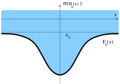
Figure 1: The spectrum of $H_{0}(x)$ for $N=2$. The thick line indicates the eigenvalue $E_{0}(x)$ sitting at the bottom of continuous spectrum.

The key observation for the following is that the interaction Hamiltonian depends only on the configuration $x$ of the particles and that the operator

$$H_{0}(x)={\rm d}\Gamma(|k|)+\sum_{j=1}^{N}H_{{\rm I},j}(x)\,,$$

which acts on $\mathcal{F}$ for fixed $x\in{\mathbb{R}}^{3N}$, has a unique ground state $\Omega(x)$ with ground state energy

$$E_{0}(x)=\sum_{j=2}^{N}\sum_{i=1}^{j-1}V_{ij}(x_{i}-x_{j})+e_{0}\,,$$ (13)

where

$$V_{ij}(z)=-\int_{{\mathbb{R}}^{3}\times{\mathbb{R}}^{3}}dv\,dw\,\frac{\rho_{i}(v-z)\rho_{j}(w)}{4\pi|v-w|}$$ (14)

and

$$e_{0}=-\frac{1}{2}\sum_{j=1}^{N}\int_{{\mathbb{R}}^{3}\times{\mathbb{R}}^{3}}dv\,dw\,\frac{\rho_{j}(v)\rho_{j}(w)}{4\pi|v-w|}\,.$$ (15)

$V_{ij}(z)$ is the electrostatic interaction energy of the charge distributions $\rho_{i}$ and $\rho_{j}$ at distance $z$, however, with the “wrong” sign. It is a peculiarity of the scalar field that the interaction between charges with equal sign is attractive. $e_{0}$ is the sum of all self energies. The remainder of the spectrum is purely absolutely continuous and the ground state energy is not isolated, cf. Figure 1.

Let $P_{*}(x)=|\Omega(x)\rangle\langle\Omega(x)|$, then the states in

$${\rm Ran}\,P_{*}=\left\{\int^{\oplus}_{{\mathbb{R}}^{3N}}dx\,\psi(x)\Omega(x):\,\,\psi\in L^{2}({\mathbb{R}}^{3N})\right\}\subset\mathcal{H}$$ (16)

correspond to wave packets without free bosons. If the particles are moving at small speeds and if the accelerations are also small, one expects that no free bosons are created, i.e. that Ran$P_{*}$ is approximately invariant under the dynamics generated by $H^{\varepsilon}$. Moreover the wave function $\psi(x)$ of the particles should approximately be governed by the effective Schrödinger equation (12) with

$$H^{\varepsilon}_{\rm eff}=\sum_{j=1}^{N}\,\sqrt{-\varepsilon^{2}\Delta_{x_{j}}+1}+\sum_{j=2}^{N}\sum_{i=1}^{j-1}V_{ij}(x_{i}-x_{j})\,.$$

Our main result, Theorem 7, states that for $\Psi_{0}=\int^{\oplus}dx\,\psi_{0}(x)\Omega(x)\in$ Ran$P_{*}$ we have

$$\Big{\|}e^{-iH^{\varepsilon}t/\varepsilon}\Psi_{0}-\int^{\oplus}_{{\mathbb{R}}^{3N}}dx\left(e^{-iH_{\rm eff}^{\varepsilon}t/\varepsilon}\,\psi_{0}\right)(x)\,e^{-ie_{0}t/\varepsilon}\,\Omega(x)\Big{\|}=\mathcal{O}(\varepsilon\sqrt{\ln(1/\varepsilon)})\,(1+|t|)\,\|\Psi_{0}\|\,.$$ (17)

Notice that in the approximate solution of the full Schrödinger equation the state of the field is, up to a fast oscillating global phase $e^{-ie_{0}t/\varepsilon}$, adiabatically following the motion of the particles. In particular, there are no bosons traveling back and forth between the particles and the phrase that the particles “interact through the exchange of bosons”, which comes from perturbation theory, should not be taken literally in the present setting.

As mentioned before, there is a strong similarity to the time-dependent Born-Oppenheimer approximation, where one obtains an effective Schrödinger equation for the nuclei in a molecule with an effective potential generated by the electrons [20]. In both cases the physical mechanism which leads to the approximate invariance of the subspace Ran$P_{*}$ is adiabatic decoupling. I.e. the separation of time scales for the motion of the different parts of the system lets the fast degrees of freedom, in our case the bosons, instantaneously adjust to the motion of the slow degrees of freedom, the particles.

However, for massless bosons – in contrast to the Born-Oppenheimer approximation – there is no spectral gap which pointwise separates the energy band $E_{0}=\{(x,E_{0}(x)):x\in{\mathbb{R}}^{3N}\}$ from the remainder of the spectrum of $H_{0}(x)$, but $E_{0}$ lies at the bottom of continuous spectrum. Hence we need a space-adiabatic theorem, cf. [20, 21, 15], without gap condition. Only recently time-adiabatic theorems without a gap condition were established in [2, 4, 22]. The notion time-adiabatic refers to the setting where the Hamiltonian of the system is itself time-dependent and varies on a slow time scale. In Section 2 a general space-adiabatic theorem without gap condition is formulated and proved. The proof is based on ideas developed in [22] and our approach gives, in particular, good control on the rate of convergence in the adiabatic limit.

As an application of the result from Section 2 we consider in Section 3 the scaling limit $\varepsilon\to 0$ of the massless Nelson model as described above. We emphasize at this point that, in view of the missing gap condition, the rate of convergence $\mathcal{O}(\varepsilon\sqrt{\ln(1/\varepsilon)})$ in (17) is surprisingly fast, since it is almost as good as in the case with a gap. Moreover, if all particles have individually total charge equal to zero, then the rate is exactly $\mathcal{O}(\varepsilon)$ as in the case with a gap. Hence, the logarithmic correction must be attributed to the Coulombic long range character of the interparticle interaction. In the situation with gap it is known [13, 15] that the wave function stays in a subspace Ran$P_{*}^{\varepsilon}$ which is $\varepsilon$-close to the band subspace Ran$P_{*}$ up to an error of order $\mathcal{O}(\varepsilon^{\infty})$. However, in the situation without gap, we expect that a piece of order $\varepsilon^{\alpha}$, $\alpha<\infty$, of the wave function is “leaking out” of Ran$P_{*}$ in the sense that it becomes orthogonal to Ran$P_{*}$ under time evolution. Physical considerations suggest that $\alpha=3/2$ for the present problem, see Remark 9. As a consequence, the $\varepsilon^{2}$ corrections to the effective Hamiltonian are still dominating dissipation and can be formally derived from the results in [15]. The effective Hamiltonian (55) then contains a renormalized mass term and the momentum dependent Darwin interaction.

Finally let us compare our results to those obtained by Davies [6], who considers the limit $c\to\infty$ for the Hamiltonian

$$H^{c}=H_{\rm p}\otimes{\bf 1}+{\bf 1}\otimes{\rm d}\Gamma(c|k|)+\sqrt{c}H_{\rm I}\,.$$ (18)

Notice that $H^{c}$ is obtained through canonical quantization of (1) and (2) if one does not set $c=1$ as we did before. Davies proves that for all $t\in{\mathbb{R}}$

$${\rm s}-\lim_{c\to\infty}e^{-iH^{c}t}(\psi\otimes\Omega)=(e^{-i(H_{\rm eff}+e_{0})t}\psi)\otimes\Omega\,,$$

where $\Omega=\{1,0,0,\ldots\}$ denotes the Fock vacuum and $H_{\rm p}:=H^{\varepsilon=1}_{\rm p}$ and $H_{\rm eff}:=H^{\varepsilon=1}_{\rm eff}$. This shows that although the limit $c\to\infty$ is equivalent to our scaling on the classical level, the results for the quantum model differ qualitatively. While we obtain effective dynamics for states which contain a nonzero number of bosons independent of $\varepsilon$, cf. (17), the $c\to\infty$ limit yields effective dynamics for states which contain no bosons at all. Furthermore, the limit $\varepsilon\to 0$ is a singular limit as no limiting dynamics for $\varepsilon=0$ exists.

In Section 3 we also consider an infrared-renormalized model suggested in [1] and [12], which allows us to do without the global infrared condition (9). The results are exactly the same as in the standard Nelson model.

2 A space-adiabatic theorem without gap condition

Generalizing from the time-adiabatic theorem of quantum mechanics [9], we consider perturbations of self-adjoint operators $H_{0}$, which are fibered over the base space ${\mathbb{R}}^{n}$, where, for better readability, we use $M:={\mathbb{R}}^{n}$ to denote this base space. Let $\mathcal{H}_{\rm f}$ be a separable Hilbert space and let $dx$ denote Lebesgue measure. Recall that $H_{0}$ acting on $\mathcal{H}=L^{2}(M,dx)\otimes\mathcal{H}_{\rm f}=L^{2}(M,dx;\mathcal{H}_{\rm f})$ is called fibered, cf. [18], if there is a measurable map $M\ni x\mapsto H_{0}(x)$ with values in the self-adjoint operators on $\mathcal{H}_{\rm f}$ such that

$$H_{0}=\int^{\oplus}_{M}\,dx\,H_{0}(x)\,.$$

There seems to be no standard name for the set

$$\Sigma=\Big{\{}(x,s)\in M\times{\mathbb{R}},s\in\sigma(H_{0}(x))\Big{\}}$$

and we propose to call it the fibered spectrum of $H_{0}$.

Let $\sigma_{*}\subset\Sigma$ be such that $x\mapsto P_{*}(x)$ is measurable, where $P_{*}(x)$ denotes the spectral projection of $H_{0}(x)$ associated with $\sigma_{*}(x)$. Then $P_{*}=\int^{\oplus}_{M}\,dx\,P_{*}(x)$ is an orthogonal projection which commutes with $H_{0}$, but which is in general not a spectral projection of $H_{0}$.

We consider perturbations of $H_{0}$, which mix the fibers, in a sense, slowly. As a prototype consider for a sufficiently regular real valued function $h$ on “momentum space” ${\mathbb{R}}^{n}$ the self-adjoint operator $h^{\varepsilon}=h(-i\varepsilon\nabla_{x})$ on $L^{2}(M)$. Here $\varepsilon>0$ is the adiabatic parameter and $[h^{\varepsilon}\otimes{\bf 1},A]=\mathcal{O}(\varepsilon)$ for any operator $A$ which is fibered over $M$. Let

$$H^{\varepsilon}=H_{0}+h^{\varepsilon}\otimes{\bf 1}\,,$$

then the invariant subspaces for $H_{0}$ constructed above are still “approximately” invariant for $H^{\varepsilon}$ with $\varepsilon$ small, since $[H^{\varepsilon},P_{*}]=\mathcal{O}(\varepsilon)$ and thus $[e^{-iH^{\varepsilon}s},P_{*}]=\mathcal{O}(\varepsilon|s|)$. But the relevant time scale for the dynamics generated by $h^{\varepsilon}$ is ${t}/{\varepsilon}$ with $t=\mathcal{O}(1)$. Thus the unitary group of interest is $e^{-iH^{\varepsilon}{t}/{\varepsilon}}$. However, according to the naive argument, $[e^{-iH^{\varepsilon}{t}/{\varepsilon}},P_{*}]=O(|t|)$ and the subspaces Ran$P_{*}$ seem to be not even approximately invariant as $\varepsilon\to 0$.

It is well known [20, 21] that the failure of the naive argument can be cured if $\sigma_{*}$ is separated by a gap from the remainder of the fibered spectrum $\Sigma$. Then $[e^{-iH^{\varepsilon}{t}/{\varepsilon}},P_{*}]=\mathcal{O}(\varepsilon)\,(1+|t|)$, a result that was baptized space-adiabatic theorem in [20]. The object of this section is to establish an analogous result without assuming a gap condition.

We remark that the general setup for space-adiabatic theory are Hamiltonians which are “fibered” over phase space, in the sense that they can be written as quantizations of operator valued symbols [15].

2.1 Assumptions and results

Let $H_{0}(x)$, $x\in M$, be a family of self-adjoint operators on some common dense domain $\mathcal{D}\subset\mathcal{H}_{\rm f}$, $\mathcal{H}_{\rm f}$ a separable Hilbert space. Let $\|\cdot\|_{H_{0}(x)}$ denote the graph norm of $H_{0}(x)$ on $\mathcal{D}$, i.e., for $\psi\in\mathcal{D}$, $\|\psi\|_{H_{0}(x)}=\|H_{0}(x)\psi\|+\|\psi\|$. We assume that all the $H_{0}(x)$-norms are equivalent in the sense that there is an $x_{0}\in M$ and constants $C_{1},C_{2}<\infty$ such that $C_{1}\|\psi\|_{H_{0}(x_{0})}\leq\|\psi\|_{H_{0}(x)}\leq C_{2}\|\psi\|_{H_{0}(x_{0})}$. Then

$$H_{0}=\int_{M}^{\oplus}\,dx\,H_{0}(x)$$

with domain $D(H_{0})=L^{2}(M)\otimes\mathcal{D}$ is self-adjoint, where here and in the following $\mathcal{D}$ resp. $D(H_{0})$ are understood to be equipped with the $\|\cdot\|_{H_{0}(x_{0})}$ resp. $\|\cdot\|_{H_{0}}$ norm. For $k\in{\mathbb{N}}_{0}$ and $\mathcal{E}$ some Banach space let

$$C_{\rm b}^{k}({\mathbb{R}}^{n},\mathcal{E})=\left\{f\in C^{k}({\mathbb{R}}^{n},\mathcal{E}):\sup_{x\in{\mathbb{R}}^{n}}\|\partial^{\alpha}_{x}f(x)\|_{\mathcal{E}}<\infty\quad\forall\,\alpha\in{\mathbb{N}}^{n}\quad{\rm with}\quad|\alpha|\leq k\right\}\,.$$

$\mathcal{L}(\mathcal{H}_{1},\mathcal{H}_{2})$ denotes the space of bounded linear operators from $\mathcal{H}_{1}$ to $\mathcal{H}_{2}$ and $\mathcal{L}_{\rm sa}(\mathcal{H})$ denotes the set of bounded self-adjoint operators on $\mathcal{H}$. Let $|\cdot|$ be the Euclidean norm on ${\mathbb{R}}^{n}$ and denote the Hessian of a function $A$ on ${\mathbb{R}}^{n}$ by $\nabla^{(2)}A(x)$. For the resolvent we write $R_{\lambda}(A)=(A-\lambda)^{-1}$. Let $m\geq 2$.

Assumption H${}_{0}^{m}$.

Let $H_{0}(\cdot)\in C^{m}_{\rm b}(M,\mathcal{L}(\mathcal{D},\mathcal{H}_{\rm f}))$ and for all $x\in M$ let $P_{*}(x)$ be an orthogonal projection such that $H_{0}(x)\,P_{*}(x)=E(x)\,P_{*}(x)$ with $P_{*}(\cdot)\in C^{m+1}_{\rm b}(M,\mathcal{L}(\mathcal{H}_{\rm f}))$ and $E(\cdot)\in C^{m}_{\rm b}(M,{\mathbb{R}})$.

In addition one of the following assertions holds:

1. For $1\leq j\leq n$

   $$\lim_{\delta\to 0}\,{\rm ess}\sup_{x\in M}\|\,\delta\,R_{E(x)-i\delta}(H_{0}(x))\,(\partial_{x_{j}}P_{*})(x)P_{*}(x)\|_{\mathcal{L(H}_{\rm f})}=0\,.$$ (19)

2. There is a constant $\delta_{0}>0$ and a function $\eta:[0,\delta_{0}]\to[0,\delta_{0}]$ with $\eta(\delta)\geq\delta$ and a constant $C<\infty$ such that for $\delta\in(0,\delta_{0}]$ and $1\leq j\leq n$

   $${\rm ess}\sup_{x\in M}\|\,R_{E(x)-i\delta}(H_{0}(x))\,(\partial_{x_{j}}P_{*})(x)P_{*}(x)\|_{\mathcal{L(H}_{\rm f})}\leq C\,\delta^{-1}\,\eta(\delta)\,.$$ (20)

3. In addition to (20) for $1\leq k,j\leq n$ also

   $${\rm ess}\sup_{x\in M}\left\|\partial_{x_{k}}\Big{(}\,R_{E(x)-i\delta}(H_{0}(x))(\partial_{x_{j}}P_{*})(x)P_{*}(x)\Big{)}\right\|_{\mathcal{L(H}_{\rm f})}\leq C\,\delta^{-1}\,\eta(\delta)$$ (21)

   holds.

A few remarks concerning Assumption H${}^{m}_{0}$ are in order:

• It is not assumed that $P_{*}(x)$ is the spectral projection of $H_{0}(x)$ corresponding to the eigenvalue $E(x)$. However, (19) holds pointwise in $x$ whenever $P_{*}(x)$ is the spectral projection and has finite rank, cf. Proposition 2.

• Inequality (20) is always satisfied with $\eta(\delta)=1$. For Assumption H${}^{m}_{0}$ (ii) and (iii) to have nontrivial consequences on the rate of convergence in the adiabatic theorem, $\eta(\delta)$ must satisfy $\lim_{\delta\to 0}\eta(\delta)=0$. These assumptions might look rather artificial at first sight, but turn out to be very natural in the proof and also in our application. For the simpler time-adiabatic setting, which gives rise to similar conditions, we refer the reader to [22].

• The regularity of $P_{*}(x)$ has to be assumed, since it does not follow from the regularity of $H_{0}(x)$ without the gap condition, even if $P_{*}(x)$ is spectral. The regularity of $E(x)$ follows from the one of $H_{0}(x)$ and $P_{*}(x)$ whenever $P_{*}(x)$ has finite rank, as can be seen by writing $E(x)=\mbox{tr}(H_{0}(x)P_{*}(x))/\mbox{tr}P_{*}(x)$.

The “band subspace” Ran$P_{*}$ defined through $P_{*}=\int^{\oplus}_{M}dx\,P_{*}(x)$ is invariant under the dynamics generated by $H_{0}$, since $[H_{0},P_{*}]=0$ holds by construction. We will consider perturbations $h^{\varepsilon}$ of $H_{0}$ satisfying

Assumption h^m.

For $\varepsilon\in(0,1]$ let $h^{\varepsilon}$ be a self-adjoint operator with domain $D(h)\subset\mathcal{H}$ independent of $\varepsilon$ such that $H_{0}+h^{\varepsilon}$ is essentially self-adjoint on $D(h)\cap D(H_{0})$. There exists an operator $(Dh)^{\varepsilon}\in\mathcal{L}_{\rm sa}(\mathcal{H})^{\oplus n}$ with $\sup_{\varepsilon\in(0,1]}\|\,|\,(Dh)^{\varepsilon}\,|\,\|_{\mathcal{L}(\mathcal{H})}<\infty$ satisfying:

1. There is a constant $C<\infty$ such that for each $A\in C^{m}_{\rm b}(M,\mathcal{L}(\mathcal{H}_{\rm f}))$

   $$\|[h^{\varepsilon},A]+i\,\varepsilon\,\nabla_{x}A\cdot(Dh)^{\varepsilon}\|_{\mathcal{L}(\mathcal{H})}\leq\,C\,\sum_{j=2}^{m}\,\varepsilon^{j}\sup_{x\in M,\,|\alpha|=j}\|\partial_{x}^{\alpha}A(x)\|_{\mathcal{L}(\mathcal{H}_{\rm f})}\,.$$

2. There is a constant $C<\infty$ such that

   $$\|\,|\,[(Dh)^{\varepsilon},H_{0}]\,|\,\|_{\mathcal{L}(D(H_{0}),\mathcal{H})}+\|\,|\,[(Dh)^{\varepsilon},h^{\varepsilon}]\,|\,\|_{\mathcal{L}(\mathcal{H})}\leq\varepsilon\,C\,.$$

By assumption, $H^{\varepsilon}=H_{0}+h^{\varepsilon}$ is essentially self-adjoint on $D(h)\cap D(H_{0})$ and we use its closure, again denoted by $H^{\varepsilon}$, to define for $t\in{\mathbb{R}}$

$$U^{\varepsilon}(t)=e^{-iH^{\varepsilon}t/\varepsilon}\,.$$

Since, according to Assumption h^m (i), $[H^{\varepsilon},P_{*}]=[h^{\varepsilon},P_{*}]=\mathcal{O}(\varepsilon)$, the naive argument gives $[U^{\varepsilon}(t),P_{*}]=|t|\mathcal{O}(1)$. Indeed, our aim is to cure the failure of the naive argument and to show that Ran$P_{*}$ is invariant for $U^{\varepsilon}(t)$ in the limit $\varepsilon\to 0$. To this end we will compare $U^{\varepsilon}(t)$ with the unitary group generated by

$$H^{\varepsilon}_{\rm diag}\,=\,H_{0}\,+\,P_{*}\,h^{\varepsilon}\,P_{*}\,+\,P_{*}^{\perp}\,h^{\varepsilon}\,P_{*}^{\perp}\,.$$

Also $H^{\varepsilon}_{\rm diag}$ is self-adjoint on $D(H^{\varepsilon})$ since $P_{*}(\cdot)\in C^{m}_{\rm b}(M,\mathcal{L}(\mathcal{H}_{\rm f}))$ and thus $H^{\varepsilon}-H^{\varepsilon}_{\rm diag}=P_{*}^{\perp}[h^{\varepsilon},P_{*}]P_{*}-P_{*}[h^{\varepsilon},P_{*}]P_{*}^{\perp}$ is bounded according to h^m (i). Again we abbreviate for $t\in{\mathbb{R}}$

$$U^{\varepsilon}_{\rm diag}(t)=e^{-iH^{\varepsilon}_{{\rm diag}}t/\varepsilon}\,,$$

and we have by construction that

$$\big{[}P_{*},U^{\varepsilon}_{\rm diag}(t)]=0\,,$$

i.e. Ran$P_{*}$ and Ran$P_{*}^{\perp}$ are invariant subspaces for the dynamics generated by $H^{\varepsilon}_{{\rm diag}}$.

Theorem 1.

Assume H${}_{0}^{m}$ and h^m for some $m\geq 2$. Let $\varepsilon\in(0,\delta_{0}]$, then

• H${}^{m}_{0}$ (i) implies that for $t\in{\mathbb{R}}$

  $$\lim_{\varepsilon\to 0}\Big{\|}U^{\varepsilon}(t)-U^{\varepsilon}_{\rm diag}(t)\Big{\|}_{\mathcal{L}(\mathcal{H})}=0\,,$$ (22)

• H${}^{m}_{0}$ (ii) implies that for some constant $C<\infty$ and all $t\in{\mathbb{R}}$

  $$\Big{\|}U^{\varepsilon}(t)-U^{\varepsilon}_{\rm diag}(t)\Big{\|}_{\mathcal{L}(\mathcal{H})}\leq\,C\,\eta(\varepsilon^{\frac{1}{2}})\,(1+|t|)\,,$$ (23)

• H${}^{m}_{0}$ (iii) implies that for some constant $C<\infty$ and all $t\in{\mathbb{R}}$

  $$\Big{\|}U^{\varepsilon}(t)-U^{\varepsilon}_{\rm diag}(t)\Big{\|}_{\mathcal{L}(\mathcal{H})}\leq\,C\,\eta(\varepsilon)\,(1+|t|)\,.$$ (24)

Note that in Theorem 1 the whole spectrum of possible rates of convergence between $o(1)$ and $\mathcal{O}(\varepsilon)$ as in the case with gap is covered. The estimates for the massless Nelson model as an application of Theorem 1 will show that, in principle, all rates can occur.

The following proposition shows that, assuming the first part of H${}^{m}_{0}$ but neither (i), (ii) or (iii), then Assumption H${}^{m}_{0}$ (i) always holds pointwise in $x$ if $P_{*}(x)$ is the spectral projection and has finite rank. The proof is analogous to the one of Lemma 4 in [2].

Proposition 2.

Assume H${}^{1}_{0}$ without (i), (ii) or (iii). If $P_{*}(x)$ is the spectral projection of $H_{0}(x)$ corresponding to the eigenvalue $E(x)$ and has finite rank, then

$$\lim_{\delta\to 0}\|\,\delta\,R_{E(x)-i\delta}(H_{0}(x))\,(\nabla_{x}P_{*})(x)P_{*}(x)\|_{\mathcal{L(H}_{\rm f})}=0\,.$$ (25)

Proof.

Since $P_{*}(x)$ has finite rank, the uniform statement (25) follows if we can show that $\lim_{\delta\to 0}\|\,\delta\,R_{E(x)-i\delta}(H_{0}(x))\,\psi\|=0$ for all $\psi\in\mbox{Ran}(\nabla_{x}P_{*})(x)P_{*}(x)$. We have

$$\lim_{\delta\to 0}\|\,i\,\delta R_{E(x)-i\delta}(H_{0}(x))\,\psi\|^{2}_{\mathcal{H}_{\rm f}}=\lim_{\delta\to 0}\int_{\mathbb{R}}\,\mu_{\psi}(d\lambda)\,\frac{\delta^{2}}{(\lambda-E(x))^{2}+\delta^{2}}=\mu_{\psi}(E(x))\,,$$ (26)

where $\mu_{\psi}$ denotes the spectral measure of $H_{0}(x)$ for $\psi$. Since $P_{*}(x)$ is the spectral projection on $\{E(x)\}$ and since, according to (29), Ran$(\nabla_{x}P_{*})(x)P_{*}(x)\subset$ Ran$P_{*}^{\perp}(x)$ we have $\mu_{\psi}(E(x))=0$ and thus (25). ∎

It is clear from (26) that additional information on the regularity of the spectral measure $\mu_{\psi}$ provides some control on the rate of convergence in (26). E.g., if $\mu_{\psi}(d\lambda)=\rho_{\psi}(\lambda)d\lambda$ with $\rho_{\psi}\in L^{\infty}({\mathbb{R}},d\lambda)$, then

$$\int_{\mathbb{R}}\,\mu_{\psi}(d\lambda)\,\frac{\delta^{2}}{(\lambda-E(x))^{2}+\delta^{2}}\,\leq\,\|\rho_{\psi}\|_{\infty}\,\int_{\mathbb{R}}\,d\lambda\,\frac{\delta^{2}}{(\lambda-E(x))^{2}+\delta^{2}}=\mathcal{O}(\delta)$$

and hence (20) would hold pointwise in $x$ with $\eta(\delta)=\delta^{1/2}$. In a sense, the rate $\mathcal{O}(\varepsilon\sqrt{\ln(1/\varepsilon)})$ for the massless Nelson model (17) is a consequence of the relevant spectral measure having a density $\rho(\lambda)\sim\lambda-E(x)$.

We emphasize that (25) for all $x\in M$ does not imply H${}^{m}_{0}$ (i), even in the case of compact $M$. This is because for pointwise convergence to imply uniform convergence one would need uniform equicontinuity of a sequence of functions. However, in the time-adiabatic setting it is indeed sufficient to have (25) for almost all $x\in I$, where $I\subset{\mathbb{R}}$ is the relevant time interval, see [22].

2.2 Proof of Theorem 1

We start with the standard argument and find that on $D(H^{\varepsilon})$

$$U^{\varepsilon}(t)-U^{\varepsilon}_{\rm diag}(t) = -\,U^{\varepsilon}(t)\int_{0}^{t}\,ds\,\frac{d}{ds}\left(U^{\varepsilon}(-s)\,U^{\varepsilon}_{\rm diag}(s)\right)$$

$$= -\,\frac{i}{\varepsilon}\,U^{\varepsilon}(t)\int_{0}^{t}\,ds\,U^{\varepsilon}(-s)\,\big{(}H^{\varepsilon}\,-\,H^{\varepsilon}_{\rm diag}\big{)}\,U^{\varepsilon}_{\rm diag}(s)\,,$$

where

$$H^{\varepsilon}\,-\,H^{\varepsilon}_{\rm diag}=P_{*}^{\perp}\,h^{\varepsilon}\,P_{*}\,+\,P_{*}\,h^{\varepsilon}\,P_{*}^{\perp}=P_{*}^{\perp}\,\big{[}h^{\varepsilon},P_{*}\big{]}\,P_{*}\,+\,\,\,\mathrm{adj.}\,.$$ (27)

In (27) and in the following “$\pm$ adj.” means that the adjoint operator of the first term in a sum is added resp. subtracted. Inserting h^m (i) into (27) and the result back into (2.2) one obtains

$$\left\|U^{\varepsilon}(t)-U^{\varepsilon}_{\rm diag}(t)\right\|_{\mathcal{L(H)}}\,=$$

$$= \,\left\|\,\int_{0}^{t}\,ds\,U^{\varepsilon}(-s)\,\left(P_{*}^{\perp}\,(\nabla_{x}P_{*})\,P_{*}\cdot(Dh)^{\varepsilon}\,P_{*}\,+\,\mbox{adj.}\right)U^{\varepsilon}_{\rm diag}(s)\right\|_{\mathcal{L(H)}}+\,\mathcal{O}(\varepsilon)|t|\,.$$

In (2.2) we also used that

$$(\nabla_{x}P_{*})(x)=P_{*}^{\perp}(x)(\nabla_{x}P_{*})(x)P_{*}(x)+\,\,{\rm adj.}\,,$$ (29)

which follows from $(\nabla_{x}P_{*})(x)=(\nabla_{x}P_{*}^{2})(x)=(\nabla_{x}P_{*})(x)P_{*}(x)+P_{*}(x)(\nabla_{x}P_{*})(x)$.

The nontrivial part in adiabatic theorems is to show that also the remaining term on the right hand side of (2.2) vanishes as $\varepsilon\to 0$. Assuming a gap condition, the basic idea is to express the integrand, which is $\mathcal{O}(1)$, as the time-derivative of a function that is $\mathcal{O}(\varepsilon)$ plus a remainder that is $\mathcal{O}(\varepsilon)$ and integrate, cf. [21, 20]. The key ingredient in this case would be the operator

$$F(x)=R_{E(x)}(H_{0}(x))\,(\nabla_{x}P_{*})(x)\,P_{*}(x)\,,$$ (30)

which is, according to (29), well defined and bounded if the eigenvalue $E(x)$ is separated from the rest of the spectrum of $H_{0}(x)$ by a gap and if $P_{*}(x)$ is spectral.

The definition (30) is made to give $[H_{0},F]=P_{*}^{\perp}\,\big{(}\nabla_{x}P_{*}\big{)}\,P_{*}$. However, in absence of a gap (30) is not well defined as an operator on $\mathcal{H}_{\rm f}$ and, following [22], we shift the resolvent into the complex plane and define

$$F_{\delta}(x)=R_{E(x)-i\delta}(H_{0}(x))\,P_{*}^{\perp}(x)\,(\nabla_{x}P_{*})(x)\,P_{*}(x)\,.$$

One now obtains

$$\big{[}\,H_{0}(x)\,,\,F_{\delta}(x)\,\big{]}=P_{*}^{\perp}(x)\,\big{(}\nabla_{x}P_{*}\big{)}(x)\,P_{*}(x)+Y_{\delta}(x)$$ (31)

with

$$Y_{\delta}(x)=-\,i\,\delta R_{E(x)-i\delta}(H_{0}(x))\,(\nabla_{x}P_{*})(x)\,P_{*}(x)\,.$$ (32)

Assumptions H${}^{m}_{0}$ (i), (ii) and (iii) each imply that $\lim_{\delta\to 0}\|Y_{\delta}\|_{\mathcal{L(H)}}=0$. To see this recall that for $A(\cdot)\in L^{\infty}(M,\mathcal{L(H}_{\rm f}))$ one has

$$\|A\|_{\mathcal{L(H)}}={\rm ess}\sup_{x\in{\mathbb{R}}^{n}}\|A(x)\|_{\mathcal{L(H}_{\rm f})}\,.$$

Note that for better readability we omit the Euclidean norm $|\ldots|$ in the notation and understand that $\|A\|$ always includes also the Euclidean norm if $A$ is an operator with $n$ components. Thus with (32) we can make the remainder in (31) arbitrarily small by choosing $\delta$ small enough. However, for the time being we let $\delta>0$ but carefully keep track of the dependence of all errors on $\delta$.

By assumption $H_{0}(\cdot)\in C^{m}_{\rm b}(M,\mathcal{L}(\mathcal{D},\mathcal{H}_{\rm f}))$ and $P_{*}(\cdot)\in C^{m+1}_{\rm b}(M,\mathcal{L}(\mathcal{H}_{\rm f}))$, which implies $F_{\delta}(\cdot)\in C^{m}_{\rm b}(M,\mathcal{L}(\mathcal{H}_{\rm f})^{\oplus n})$ and hence, according to h^m (i),

$$\left\|\,\big{[}h^{\varepsilon},F_{\delta}\,\big{]}\,\right\|_{\mathcal{L(H)}}\,\leq\,C\,\sum_{j=1}^{m}\,\varepsilon^{j}\sup_{|\alpha|=j}\,\|\,\partial^{\alpha}_{x}F_{\delta}\,\|_{\mathcal{L(H)}}=:\,f_{1}(\varepsilon,\delta)\,.$$ (33)

Combining (31) and (33) we obtain

$$\big{[}\,H^{\varepsilon},F_{\delta}\,\big{]}\,=\,P_{*}^{\perp}\,\big{(}\nabla_{x}P_{*}\big{)}\,P_{*}\,+\mathcal{O}(\|Y_{\delta}\|,f_{1}(\varepsilon,\delta))\,,$$ (34)

where in (34) and in the following $\mathcal{O}(a,b,c,\ldots)$ stands for a sum of operators whose norm in $\mathcal{L(H)}$ is bounded by a constant times $a+b+c+\ldots$. Defining

$$B_{\delta}=F_{\delta}\cdot(Dh)^{\varepsilon}\,P_{*}-\mbox{adj.}\,,$$

one finds with h^m (ii) and $f_{2}(\delta)=\|F_{\delta}\|_{\mathcal{L}(\mathcal{H},D(H_{0}))}$ that

$$\big{[}H^{\varepsilon},B_{\delta}\,\big{]} = \big{[}H^{\varepsilon},F_{\delta}\,\big{]}\cdot(Dh)^{\varepsilon}\,P_{*}\,+F_{\delta}\cdot\big{[}H^{\varepsilon},(Dh)^{\varepsilon}\big{]}\,P_{*}\,+F_{\delta}\cdot(Dh)^{\varepsilon}\,\big{[}H^{\varepsilon},\,P_{*}\big{]}+\,\mbox{adj.}$$ (35)

$$= P_{*}^{\perp}\,\big{(}\nabla_{x}P_{*}\big{)}\,P_{*}\cdot(Dh)^{\varepsilon}\,+\,\mbox{adj.}\,+\,\mathcal{O}(\varepsilon,\|Y_{\delta}\|,f_{1}(\varepsilon,\delta),\varepsilon f_{2}(\delta))\,.$$

Now the integrand in (2.2) can be written as the time-derivative of

$$A_{\delta}(s)=-\,i\,\varepsilon\,U^{\varepsilon}(-s)\,B_{\delta}\,U^{\varepsilon}(s)\,,$$

plus a remainder:

$$\frac{d}{ds}A_{\delta}(s) = U^{\varepsilon}(-s)\,[H^{\varepsilon},B_{\delta}]\,U^{\varepsilon}(s)\,$$ (36)

$$= U^{\varepsilon}(-s)\,\left(P_{*}^{\perp}\,\big{(}\nabla_{x}P_{*}\big{)}\,P_{*}\cdot(Dh)^{\varepsilon}\,P_{*}+\mbox{adj.}\right)U^{\varepsilon}(s)$$

$$+\,\mathcal{O}(\varepsilon,\|Y_{\delta}\|,f_{1}(\varepsilon,\delta),\varepsilon f_{2}(\delta))\,.$$

Inserting (36) into (2.2) enables us to do integration by parts,

$$\left\|U^{\varepsilon}(t)-U^{\varepsilon}_{\rm diag}(t)\right\|_{\mathcal{L(H)}}\,\leq$$ (37)

$$\leq \left\|\,\int_{0}^{t}\,ds\,\left(\frac{d}{ds}A_{\delta}(s)\right)U^{\varepsilon}(-s)\,U^{\varepsilon}_{\rm diag}(s)\,\right\|_{\mathcal{L(H)}}$$

$$\hskip 56.9055pt+\,|t|\,\mathcal{O}\Big{(}\varepsilon,\|Y_{\delta}\|,f_{1}(\varepsilon,\delta),\varepsilon f_{2}(\delta)\Big{)}$$

$$\leq \|A_{\delta}(t)\|_{\mathcal{L(H)}}+\|A_{\delta}(0)\|_{\mathcal{L(H)}}$$

$$+\left\|\,\int_{0}^{t}\,ds\,A_{\delta}(s)\left(\frac{d}{ds}U^{\varepsilon}(-s)\,U^{\varepsilon}_{\rm diag}(s)\right)\right\|_{\mathcal{L(H)}}$$

$$+\,|t|\,\mathcal{O}\Big{(}\varepsilon,\|Y_{\delta}\|,f_{1}(\varepsilon,\delta),\varepsilon f_{2}(\delta)\Big{)}$$

$$\leq C\,\varepsilon\,(2+|t|)\,\|F_{\delta}\|_{\mathcal{L(H)}}+\,|t|\,\mathcal{O}\Big{(}\varepsilon,\|Y_{\delta}\|,f_{1}(\varepsilon,\delta),\varepsilon f_{2}(\delta)\Big{)}\,.$$

For the last inequality in (37) we used that $\|A_{\delta}(t)\|_{\mathcal{L(H)}}\leq C\,\varepsilon\|F_{\delta}\|_{\mathcal{L(H)}}$ uniformly for $t\in{\mathbb{R}}$ and that

$$\frac{d}{ds}\,U^{\varepsilon}(t_{0},s)\,U^{\varepsilon}_{\rm diag}(s,t_{0})=-\frac{i}{\varepsilon}\,U^{\varepsilon}(t_{0},s)\,\big{(}H^{\varepsilon}(s)\,-\,H^{\varepsilon}_{\rm diag}(s)\big{)}\,U^{\varepsilon}_{\rm diag}(s,t_{0})$$

is bounded uniformly, according to (27) and h^m (i).

Writing out the various terms in (37) explicitly, we conclude that there is a constant $C<\infty$ such that

$$\left\|U^{\varepsilon}(t)-U^{\varepsilon}_{\rm diag}(t)\right\|_{\mathcal{L(H)}}\,\leq C\,\varepsilon\,\|F_{\delta}\|_{\mathcal{L(H)}}+C\,|t|\,\Big{(}\varepsilon+\|Y_{\delta}\|_{\mathcal{L(H)}}$$ (38)

$$+\varepsilon\,\|F_{\delta}\|_{\mathcal{L(H},D(H_{0}))}+\varepsilon\,\|F_{\delta}\|_{\mathcal{L(H)}}+\sum_{j=1}^{m}\,\varepsilon^{j}\sup_{|\alpha|=j}\|\partial^{\alpha}_{x}F_{\delta}\|_{\mathcal{L(H)}}\Big{)}\,.$$

Hence we are left to establish bounds on $F_{\delta}$, on its derivatives and on $Y_{\delta}$ in terms of $\delta$, which is the content of the following Lemma.

Lemma 3.

Assume H${}^{m}_{0}$, then $F_{\delta}(\cdot)\in C^{m}_{\rm b}(M,\mathcal{L}(\mathcal{H}_{\rm f})^{\oplus n})$ and there is a constant $C<\infty$ such that for $\delta\in(0,\delta_{0}]$

$$\|F_{\delta}\|_{\mathcal{L}(\mathcal{H},D(H_{0}))}\leq\,\frac{C}{\delta}\,\eta(\delta)\,,$$ (39)

$$\sup_{|\alpha|=j}\,\|\,\partial^{\alpha}_{x}\,F_{\delta}\,\|_{\mathcal{L}(\mathcal{H})}\leq\,\frac{C}{\delta^{j+1}}\,\eta(\delta)\quad\mbox{for}\,\,1\leq j\leq m\,.$$ (40)

In case H${}^{m}_{0}$ (i) holds, we have (39) and (40) with $\eta(\delta)=1$. Furthermore, if H${}^{m}_{0}$ (i) holds, then $\lim_{\delta\to 0}\|Y_{\delta}\|_{\mathcal{L(H)}}=0$ and if H${}^{m}_{0}$ (ii) or (iii) holds, then $\|Y_{\delta}\|_{\mathcal{L(H)}}\,\leq\,C\,\eta(\delta)$.

If H${}^{m}_{0}$ (iii) holds, then (40) can be improved to

$$\sup_{|\alpha|=j}\,\|\,\partial^{\alpha}_{x}\,F_{\delta}\,\|_{\mathcal{L}(\mathcal{H})}\leq\,\frac{C}{\delta^{j}}\,\eta(\delta)\quad\mbox{for}\,\,1\leq j\leq m\,.$$ (41)

Before we turn to the proof of Lemma 3 we finish the proof of Theorem 1. Assuming H${}^{m}_{0}$ (i), (22) follows by inserting the bounds from Lemma 3 into (38) and choosing $\delta=\delta(\varepsilon)$ such that $\lim_{\varepsilon\to 0}\delta(\varepsilon)=0$ and $\lim_{\varepsilon\to 0}\varepsilon/\delta(\varepsilon)^{2}=0$.

If H${}^{m}_{0}$ (ii) holds, then the bounds (39) and (40) inserted into (38) yield

$$\left\|U^{\varepsilon}(t)-U^{\varepsilon}_{\rm diag}(t)\right\|_{\mathcal{L(H)}}\,\leq C\,\varepsilon\,\frac{\eta(\delta)}{\delta}+C\,\Big{(}\varepsilon+\eta(\delta)+\varepsilon\,\frac{\eta(\delta)}{\delta}+\sum_{j=1}^{m}\,\varepsilon^{j}\,\frac{\eta(\delta)}{\delta^{j+1}}\Big{)}|t|\,.$$ (42)

In (42) the optimal choice is $\delta(\varepsilon)=\varepsilon^{\frac{1}{2}}$, which gives (23). Finally, the bounds (39) and (41) inserted into (38) yield

$$\left\|U^{\varepsilon}(t)-U^{\varepsilon}_{\rm diag}(t)\right\|_{\mathcal{L(H)}}\,\leq C\,\varepsilon\,\frac{\eta(\delta)}{\delta}+C\,\Big{(}\varepsilon+\eta(\delta)+\varepsilon\,\frac{\eta(\delta)}{\delta}+\sum_{j=1}^{m}\,\varepsilon^{j}\,\frac{\eta(\delta)}{\delta^{j}}\Big{)}|t|\,,$$

where the optimal choice $\delta(\varepsilon)=\varepsilon$ gives (24).

Proof of Lemma 3.

We abbreviate $R_{E(x)-i\delta}(H_{0}(x))$ as $R(\delta,x)$ in this proof and note that $R(\delta,\cdot)\in C^{m}_{\rm b}(M,\mathcal{L}(\mathcal{H}_{\rm f}))$ and thus $F_{\delta}(\cdot)\in C^{m}_{\rm b}(M,\mathcal{L}(\mathcal{H}_{\rm f})^{\oplus n})$ follow from $H_{0}(\cdot)\in C^{m}_{\rm b}(M,\mathcal{L}(\mathcal{D},\mathcal{H}_{\rm f}))$ together with $P_{*}(\cdot)\in C^{m+1}_{\rm b}(M,\mathcal{L}(\mathcal{H}_{\rm f}))$.

We start with the case H${}^{m}_{0}$ (ii), where (i) is included by making the obvious changes for $\eta(\delta)=1$. Assumption H${}^{m}_{0}$ (ii) immediately yields

$$\|F_{\delta}\|_{\mathcal{L}(\mathcal{H})}\leq\,\frac{C}{\delta}\,\eta(\delta)$$ (43)

and the bound on $Y_{\delta}$. (39) follows from $H_{0}(x)R(\delta,x)={\bf 1}+(E(x)-i\delta)R(\delta,x)$ and (43) together with the assumption that $E(x)$ is uniformly bounded.

For (40) we start by observing that

$$\nabla_{x}F_{\delta}(x) = R(\delta,x)\,\nabla_{x}\Big{(}(\nabla_{x}P_{*})(x)P_{*}(x)\Big{)}+\Big{(}\nabla_{x}R(\delta,x)\Big{)}(\nabla_{x}P_{*})(x)P_{*}(x)$$

$$= R(\delta,x)\nabla_{x}\Big{(}(\nabla_{x}P_{*})(x)P_{*}(x)\Big{)}-R(\delta,x)(\nabla_{x}H_{0}(x)-\nabla_{x}E(x))F_{\delta}(x).$$

Using (43) and the fact that $|\nabla_{x}E(x)|$ is uniformly bounded by assumption, we infer from (2.2) that

$$\|\,|\nabla_{x}F_{\delta}|\,\|_{\mathcal{L(H)}}=\sup_{x\in M}\|\,|\nabla_{x}F_{\delta}(x)|\,\|_{\mathcal{L(H}_{\rm f})}\leq C(\delta^{-1}+\delta^{-2}\eta(\delta))\,.$$

Hence (40) follows for $j=1$, since $\delta\leq\eta(\delta)$ by assumption.

By differentiating (2.2) again, we find, using a reduced notation with obvious meaning, that

$$\nabla^{(2)}F_{\delta}=-2R_{\delta}(\nabla H_{0}-\nabla E)\,\nabla F_{\delta}+R_{\delta}\,\nabla^{(2)}\Big{(}(\nabla P_{*})P_{*}\Big{)}-R_{\delta}(\nabla^{(2)}H_{0}-\nabla^{(2)}E)\,F_{\delta}\,.$$ (45)

Hence $\|\nabla^{(2)}F_{\delta}\|_{\mathcal{L(H)}}\leq C(\delta^{-3}\eta(\delta)+\delta^{-1}+\delta^{-2}\eta(\delta))$ which proves (40) for $j=2$. By repeated differentiation one finds inductively (40) for $j\leq m$.

To show (41) assuming H${}^{m}_{0}$ (iii), note that (41) holds by assumption for $j=1$ and inserted into (45) it gives $\|\nabla^{(2)}F_{\delta}\|_{\mathcal{L(H)}}\leq C(\delta^{-2}\eta(\delta)+\delta^{-1}+\delta^{-2}\eta(\delta))$. Analogously the estimates for all larger $j\leq m$ are improved by a factor of $\delta$. ∎

3 Effective dynamics for the massless Nelson model

As explained in the introduction, we consider $N$ spinless particles coupled to a scalar, massless, Bose field with an ultraviolet regularization in the interaction. This class of models is nowadays called Nelson’s model [1, 3, 11, 12] after E. Nelson [14], who studied the ultraviolet problem. We briefly complete the introduction of the model and collect some basic, well known facts.

A point in the configuration space ${\mathbb{R}}^{3N}$ of the particles is denoted by $x=(x_{1},\ldots,x_{N})$ and the Hamiltonian $H^{\varepsilon}_{\rm p}$ for the particles is defined in (5). $H^{\varepsilon}_{\rm p}$ is self-adjoint on the domain $H^{1}({\mathbb{R}}^{3N})$, the first Sobolev space.

The Hilbert space for the scalar field is the bosonic Fock space over $L^{2}({\mathbb{R}}^{3})$ defined in (6). On $D(\sqrt{\mathcal{N}})$, $\mathcal{N}$ the number operator, the annihilation operator $a(f)$ acts for $f\in L^{2}({\mathbb{R}}^{3})$ as

$$(a(f)\psi)^{(m)}(k_{1},\ldots,k_{m})=\sqrt{m+1}\int_{{\mathbb{R}}^{3}}\,dk\,\bar{f}(k)\,\psi^{(m+1)}(k,k_{1},\ldots,k_{m})\,,$$

where $\psi=(\psi^{(0)},\psi^{(1)},\psi^{(2)},\ldots)\in D(\sqrt{\mathcal{N}})$ if and only if $\sum_{m=0}^{\infty}m\|\psi^{(m)}\|^{2}<\infty$. The adjoint $a^{*}(f)$, which is also defined on $D(\sqrt{\mathcal{N}})$, is the creation operator and for $f,g\in L^{2}({\mathbb{R}}^{3})$ the operators $a(f)$ and $a^{*}(g)$ obey the canonical commutation relations (CCRs)

$$[a(f),a^{*}(g)]=\int_{{\mathbb{R}}^{3}}\,dk\,\bar{f}(k)\,g(k)=:\langle f,g\rangle\,,\quad[a(f),a(g)]=[a^{*}(f),a^{*}(g)]=0\,.$$ (46)

It is common to write $a(f)=\int_{{\mathbb{R}}^{3}}\,dk\,\bar{f}(k)\,a(k)$. The Hamiltonian of the field as defined in (7) can formally be written as

$$H_{\rm f}=\int_{{\mathbb{R}}^{3}}\,dk\,|k|\,a^{*}(k)\,a(k)\,.$$

More explicitly, on the $m$-particle sector the action of $H_{\rm f}$ is $(H_{\rm f}\psi)^{(m)}(k_{1},\ldots,k_{m})=\sum_{j=1}^{m}|k_{j}|\psi^{(m)}(k_{1},\ldots,k_{m})$, and $H_{\rm f}$ is self-adjoint on its maximal domain. For $f\in L^{2}({\mathbb{R}}^{3})$ the Segal field operator

$$\Phi(f)=\frac{1}{\sqrt{2}}\Big{(}a(f)+a^{*}(f)\Big{)}$$

is essentially self-adjoint on $D(\sqrt{\mathcal{N}})$. The field operator $\phi$ as used in (8) is related to $\Phi$ through $\phi(f)=\Phi(f/\sqrt{|k|})$. For the following it turns out to be more convenient to write the interaction Hamiltonian in terms of $\Phi$, where

$$H_{\rm I}=\Phi\Big{(}|k|\,v(x,k)\Big{)}$$

acts on the Hilbert space $\mathcal{H}=L^{2}({\mathbb{R}}^{3N})\otimes\mathcal{F}$ of the full system. We will consider two different choices for $v(x,k)$ in more detail. For the standard Nelson model (SN), as discussed in the introduction, one has

$$v_{\rm SN}(x,k)=\sum_{j=1}^{N}e^{ik\cdot x_{j}}\frac{\hat{\rho}_{j}(k)}{|k|^{3/2}}\,.$$ (47)

For the infrared-renormalized models (IR), as considered by Arai [1] and, more generally, by Lörinczi, Minlos and Spohn [12], one has

$$v_{\rm IR}(x,k)=\sum_{j=1}^{N}\left(e^{ik\cdot x_{j}}-1\right)\frac{\hat{\rho}_{j}(k)}{|k|^{3/2}}\,.$$ (48)

In both cases, the charge distribution $\rho_{j}\in L^{1}({\mathbb{R}}^{3})$ of the $j^{th}$ particle is assumed to be real-valued and spherically symmetric. As to be discussed below, cf. Remarks 4 and 6, we have to assume the infrared condition (9) for the (SN) model, but not for the (IR) model. The infrared condition implies, in particular, that the total charge of the system of $N$ particles must be zero.

The full Hamiltonian is given as the sum

$$H^{\varepsilon}=H^{\varepsilon}_{\rm p}\otimes{\bf 1}+{\bf 1}\otimes H_{\rm f}+H_{\rm I}+V_{\rm IR}\otimes{\bf 1}$$ (49)

and is essentially self-adjoint on $D(H_{\rm p}\otimes{\bf 1})\cap D({\bf 1}\otimes H_{\rm f})$ if $\sup_{x}\|\,|k|^{s}v(x,k)\,\|_{L^{2}({\mathbb{R}}^{3})}<\infty$ for $s\in\{\frac{1}{2},1\}$. Only in the (IR) model a potential $V_{\rm IR}$ is added, which acts as multiplication with the bounded, real-valued function

$$V_{\rm IR}(x)=\sum_{j,i=1}^{N}\int_{{\mathbb{R}}^{3}}dk\,\frac{\hat{\rho}_{j}(k)\hat{\rho}_{i}(k)^{*}}{|k|^{2}}e^{-ik\cdot x_{j}}+\frac{1}{2}\int_{{\mathbb{R}}^{3}}dk\,\left|\frac{\sum_{j=1}^{N}\hat{\rho}_{j}(k)}{|k|}\right|^{2}\,.$$ (50)

Remark 4.

If the charge distributions satisfy the infrared condition (9), then the (SN) Hamiltonian and the (IR) Hamiltonian are related by the unitary transformation

$$U_{\rm G}=\exp\left(-i\Phi\left(i\sum_{j=1}^{N}\frac{\hat{\rho}_{j}^{\,*}(k)}{|k|^{3/2}}\right)\right)\,,$$

cf. [1], which is related to the Gross transformation [14] for $x=0$. If the infrared condition is not satisfied, the (SN) model and the (IR) model carry two inequivalent representations of the CCRs for the field operators. Physically speaking, the transformation $U_{\rm G}$ removes the mean field that the $N$ charges would generate, if all of them would be moved to the origin. The vacuum in the (IR) representation corresponds to this removed mean field in the original representation, a fact which has to be taken care of in the interaction: for each particle the interaction term is now evaluated relative to the interaction at $x=0$, cf. (48), which makes also necessary the counter terms $V_{\rm IR}$. If the total charge of the system is different from zero, then the mean field is long range and, as a consequence, the corresponding transformation is no longer unitarily implementable. Indeed, it was shown that the (SN) Hamiltonian with confining potential does not have a ground state, cf. [11], while the (IR) Hamiltonian with the same confining potential does have a ground state, cf. [1]. $\diamondsuit$

In order to apply Theorem 1 we observe that $H_{\rm I}(x)$ acts for fixed $x\in{\mathbb{R}}^{3N}\,(\cong M)$ on $\mathcal{F}\,(\cong\mathcal{H}_{\rm f})$ and with $H_{0}(x)=H_{\rm f}+H_{\rm I}(x)+V_{\rm IR}(x)$ we have

$$H^{\varepsilon}=H^{\varepsilon}_{\rm p}\otimes{\bf 1}+\int_{M}^{\oplus}\,dx\,H_{0}(x)\quad\Big{(}\,\cong\,h^{\varepsilon}+H_{0}\,\Big{)}\,.$$

The following proposition collects some results about $H_{0}(x)$ and its ground state. Its proof is postponed to after the presentation of the the main theorem.

Proposition 5.

Assume that $v(x,\cdot)\in L^{2}({\mathbb{R}}^{3})$ for all $x\in{\mathbb{R}}^{3N}$ and that for some $n\geq 1$

1. $|\cdot|\partial^{\alpha}_{x}v(x,\cdot)\in L^{2}({\mathbb{R}}^{3})$ for all $x\in{\mathbb{R}}^{3N}$ and $0\leq|\alpha|\leq n$,

2. $\sup_{x\in{\mathbb{R}}^{3N}}\|\,\sqrt{|\cdot|}\,\partial^{\alpha}_{x}v(x,\cdot)\,\|_{L^{2}({\mathbb{R}}^{3})}<\infty$ for $0\leq|\alpha|\leq n$,

3. $\sup_{x\in{\mathbb{R}}^{3N}}\|\,\partial^{\alpha}_{x}v(x,\cdot)\,\|_{L^{2}({\mathbb{R}}^{3})}<\infty$ for $1\leq|\alpha|\leq n$.

Let Im$\langle v(x,\cdot),\nabla_{x}v(x,\cdot)\rangle_{L^{2}({\mathbb{R}}^{3})}=0$ for all $x\in{\mathbb{R}}^{3N}$ and $V_{\rm IR}(\cdot)\in C^{3}_{\rm b}({\mathbb{R}}^{3N})$. Then

• $H_{0}(x)$ is self adjoint on $\mathcal{D}=D(H_{\rm f})$ for all $x\in{\mathbb{R}}^{3N}$ and $H_{0}(\cdot)\in C^{n}_{\rm b}({\mathbb{R}}^{3N},$ $\mathcal{L}(\mathcal{D},\mathcal{F}))$, where $\mathcal{D}$ is equipped with the graph-norm of $H_{\rm f}$.

• $H_{0}(x)$ has a unique ground state $\Omega(x)$ for all $x\in{\mathbb{R}}^{3N}$ and, in particular,
  $H_{0}(x)\Omega(x)=E(x)\Omega(x)$ for

  $$E(x)=-\frac{1}{2}\int_{{\mathbb{R}}^{3}}\,dk\,|k|\,|v(x,k)|^{2}+V_{\rm IR}(x).$$ (51)

  Furthermore $\Omega(\cdot)\in C^{n}_{\rm b}({\mathbb{R}}^{3N},\mathcal{F})$.

It is straightforward to check that Im$\langle v(x,\cdot),\nabla_{x}v(x,\cdot)\rangle_{L^{2}({\mathbb{R}}^{3})}=0$ for $v_{\rm SN}$ defined in (47) and $v_{\rm IR}$ defined in (48). For the (SN) model as well as for the (IR) model (51) is easily evaluated and one finds $E(x)=E_{0}(x)$ as given in (13).

Remark 6.

For the (SN) model the assumptions made on $v(x,k)$ in Proposition 5 are satisfied, if $\hat{\rho}_{j}(k)$ decays sufficiently fast for large $|k|$ and each $j=1,\ldots,N$, or, equivalently, if $\rho_{j}(x)$ is sufficiently smooth. This is an ultraviolet condition individually for each particle. But $v(x,\cdot)\in L^{2}({\mathbb{R}}^{3})$ follows from $v(0,\cdot)\in L^{2}({\mathbb{R}}^{3})$, which is exactly the global infrared condition (9).

While the necessity for an ultraviolet regularization remains in the (IR) model, the infrared condition is replaced by $\sum_{j}|k|^{-\frac{3}{2}}\widehat{\rho}_{j}(k)(e^{ik\cdot x_{j}}-1)\in L^{2}({\mathbb{R}}^{3})$, which can be satisfied without having $\sum_{j}\widehat{\rho}_{j}(0)=0$. Thus the (IR) model allows us to consider particles with total charge different from zero. $\diamondsuit$

Let $P_{*}(x)=|\Omega(x)\rangle\langle\Omega(x)|$, then $P_{*}(\cdot)\in C^{n}_{\rm b}({\mathbb{R}}^{3N},\mathcal{L}(\mathcal{F}))$ and Ran$P_{*}$ is a candidate for an adiabatically decoupled subspace. Indeed, we will show that $h^{\varepsilon}=H^{\varepsilon}_{\rm p}\otimes{\bf 1}$ satisfies Assumption h^m with $(Dh)^{\varepsilon}_{x_{j}}=-i\varepsilon\nabla_{x_{j}}/\sqrt{-\varepsilon^{2}\Delta_{x_{j}}+1}$ and that $H_{0}$ and $P_{*}$ satisfy Assumption H${}^{m}_{0}$ (iii) with $\eta(\delta)=\delta\sqrt{\ln(1/\delta)}$ if particles with charges different from zero are present and $\eta(\delta)=\delta$ if all particles have total charge zero. Hence we can apply Theorem 1 to conclude that for some constant $C<\infty$

$$\left\|e^{-iH^{\varepsilon}t/\varepsilon}-e^{-iH^{\varepsilon}_{\rm diag}t/\varepsilon}\right\|\leq\,C\,\eta(\varepsilon)\,(1+|t|)\,,$$ (52)

with $H^{\varepsilon}_{\rm diag}=P_{*}\,H^{\varepsilon}\,P_{*}+({\bf 1}-P_{*})\,H^{\varepsilon}\,({\bf 1}-P_{*})$.

Next observe that the ground state band subspace Ran$P_{*}$ is unitarily equivalent to the Hilbert space $L^{2}({\mathbb{R}}^{3N})$ of the $N$ particles in a natural way. Let

$$\mathcal{U}:{\rm Ran}P_{*}\to L^{2}({\mathbb{R}}^{3N})\,,\quad\psi\mapsto(\mathcal{U}\psi)(x)=\langle\Omega(x),\psi(x)\rangle_{\mathcal{F}}\,,$$ (53)

then it is easily checked that for $\varphi\in L^{2}({\mathbb{R}}^{3N})$

$$\mathcal{U}^{*}\varphi=\mathcal{U}^{-1}\varphi=\int_{{\mathbb{R}}^{3N}}^{\oplus}\,dx\,\varphi(x)\,\Omega(x)\,.$$

Hence the part of $H^{\varepsilon}_{\rm diag}$ acting on Ran$P_{*}$ is unitarily equivalent to

$$\widetilde{H}^{\varepsilon}_{\rm eff}=\mathcal{U}\,P_{*}\,H^{\varepsilon}\,P_{*}\,\mathcal{U}^{*}$$

acting on the Hilbert space of the $N$ particles only. The following theorem shows that $\widetilde{H}^{\varepsilon}_{\rm eff}$ has, at leading order, exactly the form expected from the heuristic “Peierls substitution” argument.

Theorem 7.

Let $H^{\varepsilon}$ be defined as in (49) with $v(x,k)$ either $v_{\rm SN}(x,k)$ as in (47) or $v_{\rm IR}(x,k)$ as in (48). For $1\leq j\leq N$ let $\rho_{j}\in L^{1}({\mathbb{R}}^{3})$ such that $\hat{\rho}_{j}$ satisfies $|k|^{s}\widehat{\rho}_{j}(k)\in L^{2}({\mathbb{R}}^{3})$ for $s\in\{-1,4\}$. For the (SN) model assume, in addition, the infrared condition (9). Let

$$H_{\rm eff}^{\varepsilon}=H^{\varepsilon}_{\rm p}+\sum_{j=2}^{N}\sum_{i=1}^{j-1}V_{ij}(x_{i}-x_{j})+e_{0}\,,$$

with $V_{ij}(z)$ and $e_{0}$ as in (14) and (15). Then there is a constant $C<\infty$ such that

$$\Big{\|}\Big{(}e^{-iH^{\varepsilon}t/\varepsilon}-\mathcal{U}^{*}\,e^{-iH^{\varepsilon}_{\rm eff}t/\varepsilon}\,\mathcal{U}\Big{)}P_{*}\Big{\|}\leq\,C\,\eta(\varepsilon)\,(1+|t|)\,,$$ (54)

where $\eta(\varepsilon)=\varepsilon\sqrt{\ln(1/\varepsilon)}$. If all charges satisfy the infrared condition individually, i.e. if $\hat{\rho}_{j}(k)/|k|^{3/2}\in L^{2}({\mathbb{R}}^{3})$ for all $j=1,\ldots,N$, then (54) holds with $\eta(\varepsilon)=\varepsilon$.

For sake of better readability the global energy shift $e_{0}$ was, as opposed to (17), absorbed into the definition of $H_{\rm eff}^{\varepsilon}$.

Remark 8.

The unitary $\mathcal{U}$ intertwines the position operator $x\otimes{\bf 1}$ on $L^{2}({\mathbb{R}}^{3N})\otimes\mathcal{F}$ with the position operator $x$ on $L^{2}({\mathbb{R}}^{3N})$ exactly and the momentum operator $-i\varepsilon\nabla_{x}\otimes{\bf 1}$ on $L^{2}({\mathbb{R}}^{3N})\otimes\mathcal{F}$ with $-i\varepsilon\nabla_{x}$ on $L^{2}({\mathbb{R}}^{3N})$ up to an error of order $\varepsilon$. Thus one can directly read off the position distribution and approximately also the momentum distribution of the particles from the solution $\psi(t)=e^{-iH^{\varepsilon}_{\rm eff}t/\varepsilon}\psi_{0}$ of the effective dynamics. It is not necessary to transform back to the full Hilbert space using $\mathcal{U}^{*}$. $\diamondsuit$

Remark 9.

From the discussion of the introduction one expects, on physical grounds, that the energy lost through radiation is of order $\mathcal{O}(\varepsilon^{3})$ after times of order $\mathcal{O}(\varepsilon^{-1})$. Hence the error of order $\mathcal{O}(\varepsilon\sqrt{\ln 1/\varepsilon})$ in (54) is not optimal in the sense that the error does not correspond to emission of free bosons and thus to dissipation. Indeed, we expect that the situation is similar to adiabatic perturbation theory with gap, cf. [15]. There should be a subspace Ran$P^{\varepsilon}_{*}$ which is $\varepsilon$-close to Ran$P_{*}$ and for which the analogous expression to (52) holds with an error of order $\mathcal{O}(\varepsilon^{\frac{3}{2}})$, possibly with a logarithmic correction. The corresponding effective Hamiltonian would then contain two additional terms of order $\varepsilon^{2}$, which, for the case of quadratic dispersion

$$H^{\varepsilon}_{\rm p}=-\,\sum_{j=1}^{N}\frac{\varepsilon^{2}}{2}\Delta_{x_{j}}$$

for the particles, can be calculated using formula (47) in [15]. As result we obtain for the Weyl symbol of the effective Hamiltonian including the momentum dependent Darwin term

$$H_{\rm eff}(p,q)=\sum_{j=1}^{N}\frac{1}{2m_{j}^{\varepsilon}}\,p_{j}^{2}+E(q)+\frac{\varepsilon^{2}}{2}\,\sum_{j<i}\int_{{\mathbb{R}}^{3}}dk\,\frac{(p_{j}\cdot\kappa)(p_{i}\cdot\kappa)}{|k|^{2}}e^{-ik\cdot(q_{j}-q_{i})}\hat{\rho}_{j}^{*}(k)\hat{\rho}_{i}(k)$$ (55)

with $m_{j}^{\varepsilon}=1/(1+\frac{\varepsilon^{2}}{2}e_{j})$ and

$$e_{j}=\frac{1}{4\pi}\int_{{\mathbb{R}}^{3}\times{\mathbb{R}}^{3}}dv\,dw\,\frac{\rho_{j}(v)\rho_{j}(w)}{|v-w|}$$

the electromagnetic mass. As explained above, for the rigorous justification of (55) a space-adiabatic theorem without gap but for rotated subspaces $P_{*}^{\varepsilon}$ is needed and thus it is beyond the scope of the present paper. $\diamondsuit$

Before proving Theorem 7 we make up for the

Proof of Proposition 5.

A standard estimate (cf. e.g. [3] Proposition 1.3.8) shows that for $f\in L^{2}({\mathbb{R}}^{3})$ and any $a>0$

$$\|\Phi(f)\psi\|^{2}_{\mathcal{F}}\leq a\|H_{\rm f}\psi\|^{2}_{\mathcal{F}}+\left(\frac{\|f/\sqrt{|\cdot|}\,\|^{4}_{L^{2}({\mathbb{R}}^{3})}}{a}+2\right)\|\psi\|^{2}_{\mathcal{F}}\,.$$ (56)

Hence $\Phi(f)$ is infinitesimally $H_{\rm f}$-bounded whenever $\|f\|_{L^{2}({\mathbb{R}}^{3})}+\|f/\sqrt{|\cdot|}\|_{L^{2}({\mathbb{R}}^{3})}<\infty$. Then Kato-Rellich implies that $H_{0}(x)$ is self-adjoint on $D(H_{\rm f})$, since $\sqrt{|\cdot|}v(x,\cdot)\in L^{2}$ is assumed. Using (i), (ii) and $V_{\rm IR}(\cdot)\in C^{n}_{\rm b}({\mathbb{R}}^{3N})$, we obtain from (56) that

$$\partial^{\alpha}_{x}H_{0}(x)=\Phi\left(|k|\,\partial^{\alpha}_{x}v(x,k)\right)+\partial^{\alpha}_{x}V_{\rm IR}(x)$$ (57)

is relatively bounded with respect to $H_{\rm f}$ for $|\alpha|\leq n$. Moreover, (ii), (56) and (57) imply that $H_{0}(\cdot)\in C^{n}_{\rm b}({\mathbb{R}}^{3N},\mathcal{L}(\mathcal{D},\mathcal{F}))$.

To compute the ground state energy $E(x)$ observe that from “completing the square” one finds

$$H_{0}(x)=\int_{{\mathbb{R}}^{3}}dk\,|k|\,\Big{(}a^{*}(k)+\frac{v^{*}(k,x)}{\sqrt{2}}\Big{)}\Big{(}a(k)+\frac{v(x,k)}{\sqrt{2}}\Big{)}-\frac{1}{2}\int_{{\mathbb{R}}^{3}}dk\,|k|\,|v(x,k)|^{2}+V_{\rm IR}(x)\,.$$

It is well known that the map $a(k)\mapsto a(k)+v(x,k)/\sqrt{2}$ comes from the unitary transformation $U(x)=\exp\Big{(}i\Phi\big{(}iv(x,\cdot)\big{)}\Big{)}$, i.e.

$$U(x)\,a(f)\,U^{*}(x)=a(f)+\langle f,v(x,\cdot)\rangle\,,$$ (58)

whenever $v(x,\cdot)\in L^{2}$. Equation (58) follows from the fact that $[A,[A,B]]=0$ implies $[\exp(iA),B]=\exp(iA)[iA,B]$ and the CCRs. Transformations of the form (58) are called Bogoliubov transformations.

Therefore $H_{0}(x)=U(x)\,H_{\rm f}\,U^{*}(x)\,+E(x)$ with $E(x)=-\frac{1}{2}\int_{{\mathbb{R}}^{3}}\,dk\,|k|\,|v(x,k)|^{2}+V_{\rm IR}(x)$. Since $H_{\rm f}\,\Omega_{0}=0$ for the unique ground state $\Omega_{0}=(1,0,0,\ldots)\in\mathcal{F}$, we find

$$H_{0}(x)\Omega(x)=E(x)\Omega(x)\quad\mbox{with}\quad\Omega(x)=U(x)\Omega_{0}\,.$$

Next we need to take derivatives of $U(x)$ with respect to $x$. It follows from the CCRs (46) that for $f,g\in L^{2}({\mathbb{R}}^{3})$

$$\big{[}\Phi(f),\Phi(g)\big{]}=i\,{\rm Im}\langle f,g\rangle\,,$$

and thus, by assumption, that $\nabla_{x}\Phi(iv(\cdot,x))=\Phi(i\nabla_{x}v(\cdot,x))$ commutes with $\Phi(iv(\cdot,x))$. Hence we obtain that on $D(\sqrt{\mathcal{N}})$

$$\nabla_{x}U(x)=U(x)\,i\Phi(i\nabla_{x}v(\cdot,x))=i\Phi(i\nabla_{x}v(\cdot,x))\,U(x)\,.$$ (59)

By further differentiating (59) we can get up to $n^{th}$ derivatives since $\partial_{x}^{\alpha}v(x,k)\in L^{2}({\mathbb{R}}^{3})$ for $|\alpha|\leq n$. In particular we find with (iii) that $\Omega(x)=U(x)\Omega_{0}\in C^{n}_{\rm b}({\mathbb{R}}^{3N},\mathcal{F})$. ∎

Proof of Theorem 7.

We start by showing that the assumptions of Theorem 1 are indeed satisfied and thus (52) follows.

It is straightforward to check that the assumptions on $\hat{\rho}_{j}$ imply the assumptions of Proposition 5 for $n=5$. Hence the first part of H${}_{0}^{4}$ follows with $P_{*}(x)=|\Omega(x)\rangle\langle\Omega(x)|$. For H${}_{0}^{4}$ (iii) observe that, using (59), $\nabla_{x}\Omega(x)=\nabla_{x}U(x)\Omega_{0}=U(x)\,i\Phi(i\nabla_{x}v(\cdot,x))\Omega_{0}$, and thus

$$\langle\Omega(x),\nabla_{x}\Omega(x)\rangle_{\mathcal{F}}=\langle\Omega_{0},i\Phi(i\nabla_{x}v(\cdot,x))\Omega_{0}\rangle_{\mathcal{F}}=0\,.$$ (60)

As a consequence, $(\nabla_{x}P_{*})(x)P_{*}(x)=|\nabla_{x}\Omega(x)\rangle\langle\Omega(x)|$. Hence we obtain for $1\leq j\leq N$

$$R(\delta,x)(\nabla_{x_{j}}P_{*})(x)P_{*}(x)=i\,|U(x)\,R_{\rm f}(\delta)\,\Phi(i\nabla_{x_{j}}v(\cdot,x))\Omega_{0}\rangle\langle\Omega(x)|\,,$$ (61)

where $R_{\rm f}(\delta)=(H_{\rm f}-i\delta)^{-1}$. For (20) one therefore finds

$$\|R(\delta,x)(\nabla_{x_{j}}P_{*})(x)P_{*}(x)\|^{2}_{\mathcal{L(F)}} = \|R_{\rm f}(\delta)\Phi(i\nabla_{x_{j}}v(x,\cdot))\Omega_{0}\|^{2}_{\mathcal{F}}$$ (62)

$$= \left\|(|k|-i\delta)^{-1}k\,e^{ik\cdot x_{j}}\hat{\rho}_{j}(k)|k|^{-\frac{3}{2}}\right\|^{2}_{L^{2}({\mathbb{R}}^{3})}$$

Whenever $\rho_{j}$ satisfies the infrared condition $\hat{\rho}_{j}(k)|k|^{-\frac{3}{2}}\in L^{2}({\mathbb{R}}^{3})$, (62) is bounded uniformly in $\delta$ since $\big{|}\,|k|/(|k|-i\delta)\,\big{|}\leq 1$. In general we only assume that $\hat{\rho}_{j}(k)|k|^{-1}\in L^{2}({\mathbb{R}}^{3})$. Using that $\hat{\rho}_{j}(k)$ is bounded uniformly according to Riemann-Lebesgue, (62) becomes

$$\left\|(|k|-i\delta)^{-1}k\,e^{ik\cdot x_{j}}\hat{\rho}_{j}(k)|k|^{-\frac{3}{2}}\right\|^{2}_{L^{2}({\mathbb{R}}^{3})}\leq C_{1}\,\int_{0}^{1}\,d|k|\frac{|k|}{|k|^{2}+\delta^{2}}+C_{2}\leq C\ln{1/\delta}\,,$$ (63)

for $\delta\in(0,\textstyle{\frac{1}{2}}]$. To obtain the estimate (21), we differentiate (61) and find

$$\nabla_{x_{i}}\Big{(}R(\delta,x)(\nabla_{x_{j}}P_{*})(x)P_{*}(x)\Big{)}=i\,|U(x)\,R_{\rm f}(\delta)\Phi(i\nabla_{x_{j}}v(x,\cdot))\Omega_{0}\rangle\langle\nabla_{x_{i}}\Omega(x)|$$ (64)

$$-\,\,|U(x)\,\Phi(i\nabla_{x_{i}}v(x,\cdot))\,R_{\rm f}(\delta)\Phi(i\nabla_{x_{j}}v(x,\cdot))\Omega_{0}\rangle\langle\Omega(x)|$$

$$+\,\,i\,|U(x)\,R_{\rm f}(\delta)\Phi(i\nabla^{(2)}_{ij}v(x,\cdot))\Omega_{0}\rangle\langle\Omega(x)|\,.$$

All three terms in (64) can be bounded by using the same type of arguments as in (62) and (63): For the first term use in addition that $\|\nabla_{x_{i}}\Omega(x)\|_{\mathcal{H}_{\rm f}}<C$ and for the second term one has to estimate the components in the $0$-boson sector and in the $2$-boson sector separately. In summary we showed that H${}_{0}^{4}$ (iii) is satisfied with $\eta(\delta)=\delta\sqrt{\ln(1/\delta)}$, and with $\eta(\delta)=\delta$ if all charges satisfy the infrared condition individually.

We are left to check for Assumption h⁴. Let $h^{\varepsilon}=H_{\rm p}^{\varepsilon}\otimes{\bf 1}=\sum_{j}h(-i\varepsilon\nabla_{x_{j}})\otimes{\bf 1}$, with $h(p)=\sqrt{p^{2}+1}$. Essential self-adjointness of $h^{\varepsilon}+H_{0}$ on $D(H_{\rm p}\otimes{\bf 1})\cap D(H_{0})$ is a standard result, cf. Proposition 2.1 in [1]. We define $(Dh)^{\varepsilon}_{j}=(\nabla h)(-i\varepsilon\nabla_{x_{j}})\otimes{\bf 1}$, with $\|(Dh)^{\varepsilon}\|_{\mathcal{L(H)}^{\oplus\,3N}}\leq 1$, and postpone the technical proof of the following Lemma to the end of this section.

Lemma 10.

$h^{\varepsilon}$ and $(Dh)^{\varepsilon}$ satisfy h⁴ (i) and (ii).

We conclude that all assumptions of Theorem 1 are satisfied for the (SN) and the (IR) model and thus (52) holds. However, (54) follows from (52) by the following Lemma and an argument like (2.2). ∎

Lemma 11.

There is a constant $C<\infty$ such that for $\varepsilon>0$ sufficiently small

$$\left\|\left(H^{\varepsilon}_{\rm diag}\,-\,\mathcal{U}^{*}\,H^{\varepsilon}_{\rm eff}\,\mathcal{U}\,\right)\,P_{*}\,\right\|_{\mathcal{L(H)}}\leq\,\varepsilon^{2}\,C\,.$$

Proof.

In order to apply h⁴ (i) to $\mathcal{U}(x)$, we have to extend $\mathcal{U}(x):\mbox{Ran}P_{*}(x)\to{\mathbb{C}}$ defined in (53) to a map $\widetilde{\mathcal{U}}(\cdot)\in C^{4}_{\rm b}({\mathbb{R}}^{3N},\mathcal{L(F)})$ first. To this end let $\widetilde{\mathcal{U}}(x)=|\Omega_{0}\rangle\langle\Omega(x)|$ and note that $\widetilde{\mathcal{U}}^{*}\,\widetilde{\mathcal{U}}=P_{*}$. With this definition one finds

$$H^{\varepsilon}_{\rm diag}\,P_{*} = H_{0}\,P_{*}+P_{*}\,h^{\varepsilon}\,P_{*}=E\,P_{*}+P_{*}\,\widetilde{\mathcal{U}}^{*}\,h^{\varepsilon}\,\widetilde{\mathcal{U}}\,P_{*}+P_{*}\,[\,h^{\varepsilon},\,\widetilde{\mathcal{U}}^{*}\,]\,\widetilde{\mathcal{U}}\,P_{*}$$

$$= \mathcal{U}^{*}\,H^{\varepsilon}_{\rm eff}\,\mathcal{U}\,P_{*}+P_{*}\,[\,h^{\varepsilon},\,\widetilde{\mathcal{U}}^{*}\,]\,\widetilde{\mathcal{U}}\,P_{*}\,,$$

and we are left to show that $\|P_{*}\,[\,h^{\varepsilon},\,\widetilde{\mathcal{U}}^{*}\,]\,\widetilde{\mathcal{U}}\,P_{*}\|=\mathcal{O}(\varepsilon^{2})$. Using h⁴ (i) with $A=\widetilde{\mathcal{U}}^{*}$ we find that

$$P_{*}\,[\,h^{\varepsilon},\,\widetilde{\mathcal{U}}^{*}\,]\,\widetilde{\mathcal{U}}\,P_{*}=-i\varepsilon\,P_{*}\,(\nabla_{x}\,\widetilde{\mathcal{U}}^{*})\cdot(Dh)^{\varepsilon}\,\widetilde{\mathcal{U}}\,P_{*}+\mathcal{O}(\varepsilon^{2})\,.$$

However, according to (60)

$$P_{*}(x)(\nabla_{x}\,\widetilde{\mathcal{U}}^{*})(x)=|\Omega(x)\rangle\langle\Omega(x),\,\nabla_{x}\,\Omega(x)\rangle\langle\Omega_{0}|=0\,,$$

and thus the desired result follows. ∎

Proof of Lemma 10.

Heuristically h⁴ (i) and (ii) hold, because they are just special cases of the expansion of a commutator of pseudodifferential operators. However, since $h^{\varepsilon}$ is unbounded and $A$ is only 4-times differentiable, we need to check the estimates “by hand”.

For notational simplicity we restrict ourselves to the case $N=1$, from which the general case follows immediately. Let $g(p)=1/\sqrt{p^{2}+1}$, $g^{\varepsilon}=g(-i\varepsilon\nabla_{x})\otimes{\bf 1}$ and $A\in C_{\rm b}^{4}({\mathbb{R}}^{3},\mathcal{H}_{\rm f})$, then $|\cdot|^{s}\widehat{g}\in L^{1}({\mathbb{R}}^{3})$ for $s\in\{0,4\}$ and thus for $\psi\in\mathcal{S}$

$$\Big{(}g^{\varepsilon}A\psi\Big{)}(x)=\int dy\,\widehat{g}(y)\,A(x-\varepsilon y)\,\psi(x-\varepsilon y)$$ (65)

$$= \int dy\,\widehat{g}(y)\,\left(A(x)-\varepsilon y\cdot\nabla A(x)+\varepsilon^{2}\int_{0}^{1}ds\,\langle y,\nabla^{(2)}A(x-s\varepsilon y)\,y\rangle\right)\psi(x-\varepsilon y)$$

$$= \Big{(}Ag^{\varepsilon}\psi\Big{)}(x)-i\,\varepsilon\Big{(}\nabla A\cdot\nabla g^{\varepsilon}\psi\Big{)}(x)$$

$$\hskip 56.9055pt+\,\int dy\,\widehat{g}(y)\,\varepsilon^{2}\int_{0}^{1}ds\,\langle y,\nabla^{(2)}A(x-s\varepsilon y)\,y\rangle\psi(x-\varepsilon y)\,.$$

From (65) one concludes after a lengthy but straightforward computation involving several integrations by parts that

$$\varepsilon^{2}\Delta_{x}\,[g^{\varepsilon},A]=-i\,\varepsilon\nabla A\cdot(\nabla g)^{\varepsilon}\,(\varepsilon^{2}\Delta_{x})+R$$

with

$$\|R\,\|\leq\,C\,\sum_{j=2}^{4}\,\varepsilon^{j}\sup_{x\in{\mathbb{R}}^{3N},\,|\alpha|=j}\|\partial_{x}^{\alpha}A(x)\|_{\mathcal{L}(\mathcal{H}_{\rm f})}\,.$$

Hence we find

$$[h^{\varepsilon},A]=[(1-\varepsilon^{2}\Delta_{x})g^{\varepsilon},A]=(1-\varepsilon^{2}\Delta_{x})[g^{\varepsilon},A]-[\varepsilon^{2}\Delta_{x},A]g^{\varepsilon}=-i\,\varepsilon\nabla A\cdot(Dh)^{\varepsilon}+R^{\prime}$$

with

$$\|R^{\prime}\,\|\leq\,C^{\prime}\,\sum_{j=2}^{4}\,\varepsilon^{j}\sup_{x\in{\mathbb{R}}^{3N},\,|\alpha|=j}\|\partial_{x}^{\alpha}A(x)\|_{\mathcal{L}(\mathcal{H}_{\rm f})}\,.$$

This proves h⁴ (i). By the same type of arguments one shows also h⁴ (ii). ∎

Acknowledgments. I am grateful to Herbert Spohn for suggesting the massless Nelson model as an application for a space-adiabatic theorem without gap, as well as for numerous valuable discussions, remarks and hints concerning the literature. Parts of this work developed during a stay of the author at the Univerité de Lille and I thank Stephan De Bièvre and Laurent Bruneau for hospitality and for a helpful introduction to Reference [1]. For critical remarks which lead to an improved presentation a thank Detlef Dürr.

References

[1] A. Arai. Ground state of the massless Nelson model without infrared
cutoff in a non-Fock representation, Rev. Math. Phys. 13, 1075–1094 (2001).
[2] J.E. Avron and A. Elgart. Adiabatic theorem without a gap condition,
Commun. Math. Phys. 203, 445–463 (1999).
[3] V. Betz. Gibbs measures relative to Brownian motion and Nelson’s
model, Dissertation, TU München (2002).
[4] F. Bornemann. Homogenization in time of singularly perturbed
mechanical systems,
Lecture Notes in Mathematics 1687, Springer, Heidelberg, 1998.
[5] T. Chen. Operator-theoretic infrared renormalization
and construction of dressed -particle states in non-relativistic QED,
Dissertation, ETH Zürich No. 14203 (2001).
[6] E. B. Davies. Particle-boson interactions and the weak coupling
limit, J. Math. Phys. 20, 345–351 (1979).
[7] J. Fröhlich. On the infrared problem in a model of scalar electrons
and massless scalar bosons, Ann. Inst. Henri Poincaré 19, 1–103 (1973).
[8] F. Hiroshima. Weak coupling limit with a removal
of an ultraviolet cutoff for a Hamiltonian of particles interacting with
a massive scalar field, Inf. Dim. Anal., Quant. Prob. and Related Topics
1, 407–423 (1998).
[9] T. Kato. On the adiabatic theorem of quantum
mechanics, Phys. Soc. Jap. 5, 435–439 (1958).
[10] M. Kunze and H. Spohn.
Slow motion of charges interacting through the Maxwell field, Commun. Math. Phys. 203, 1–19 (2000).
[11] J. Lörinczi, R. A. Minlos and H. Spohn. The infrared behavior
in Nelson’s model of a quantum particle coupled to a massless scalar field, Ann. Henri
Poincaré 3, 1–28 (2002).
[12] J. Lörinczi, R. A. Minlos and H. Spohn. Infrared regular
representation of the three dimensional massless Nelson model, to appear in Lett. Math. Phys. (2001).
[13] A. Martinez and V. Sordoni. On the
time-dependent Born-Oppenheimer approximation with smooth potential,
to appear in Comptes Rendus (2001).
[14] E. Nelson.
Interaction of nonrelativistic particles with a quantized scalar
field, Jour. Math. Phys. 5, 1190–1197 (1964).
[15] G. Panati, H. Spohn and S. Teufel. Space-adiabatic perturbation theory,
preprint, mp_arc 02-34 (2002).
[16] G. Panati, H. Spohn and S. Teufel. Space-adiabatic decoupling
to all orders, preprint, quant-ph/0201123 (2002).
[17] M. Reed and B. Simon. Methods of modern mathematical
physics II, Academic Press (1975).
[18] M. Reed and B. Simon. Methods of modern mathematical
physics IV, Academic Press (1978).
[19] H. Spohn. Dynamics of charged particles and their radiation field,
in preparation.
[20] H. Spohn and S. Teufel. Adiabatic decoupling and
time-dependent Born-Oppenheimer theory, Commun. Math. Phys. 224,
113–132 (2001).
[21] S. Teufel and H. Spohn. Semiclassical motion of
dressed electrons, Rev. Math. Phys. 4, 1–28 (2002).
[22] S. Teufel. A note on the adiabatic theorem without gap condition,
to appear in Lett. Math. Phys. (2001).