SUPERMANIFOLDS – APPLICATION TO SUPERSYMMETRY

Abstract

Parity is ubiquitous, but not always identified as a simplifying tool for computations. Using parity, having in mind the example of the bosonic/fermionic Fock space, and the framework of ${\mathbb{Z}}_{2}$-graded (super) algebra, we clarify relationships between the different definitions of supermanifolds proposed by various people. In addition, we work with four complexes allowing an invariant definition of divergence:

• an ascending complex of forms, and a descending complex of densities on real variables

• an ascending complex of forms, and descending complex of densities on Graßmann variables.

This study is a step towards an invariant definition of integrals of superfunctions defined on supermanifolds leading to an extension to infinite dimensions. An application is given to a construction of supersymmetric Fock spaces.

1 Dedication

Three quotes from M.S. Marinov.
1. Particle spin dynamics as the Graßmann variant of classical mechanics, F.A. Berezin and M.S. Marinov, Annals of Physics 104, 336–362 (1977).

During the past few years a not so familiar concept has emerged in high-energy physics, that of “anticommuting $c$-numbers.”  The formalism of the Graßmann algebra is well known to mathematicians and has been used for a long time. The analysis on the Graßmann algebra was developed and exploited in a systematic way in applying the generating functional method to the theory of second quantization.[11]…Seemingly, the first physical work dealing with the anticommuting numbers in connection with fermions was that by Matthews and Salam.[12]

The authors mention also the works of Gervais and Sakita,[13] and Iwasaki and Kikkawa.[14]
2. Classical spin and Graßmann algebra, F.A. Berezin and M.S. Marinov, JETP Lett., 21, 320–321 (1975).

In view of the introduction of transformation groups with anticommuting parameters into the theory of elementary particles,[15] and the intensive discussion of “supersymmetry” (see, for example, Zumino’s review [16]), universal interest has been advanced in classical anticommuting quantities, i.e., in the Graßmann-algebra formalism.

3. Path integrals in quantum theory, M.S. Marinov, Physics Reports, 60, 1–57 (1980).

As it was suggested by Schwinger [17] (for further discussion see the book [18]), the matrix determining the Poisson brackets and the canonical commutation relations, must be skew Hermitian; then the consistent classical and quantum dynamics may be constructed on the basis of the variation principle. Remarkably, not only a real and skew-symmetrical matrix (as in subsection 5.1), but also an imaginary symmetrical one is possible. However, in the second case the canonical variables should be anticommuting. Seemingly, this suggestion did not attract attention in that time, though it is very essential for understanding Schwinger’s approach to quantum electrodynamics. The analysis in a space of anticommuting variables (in the Graßmann algebra) as exhaustively developed by,[19] and used for a consistent and unified functional approach to the quantum theory with Fermi fields (see also the book by Rzewusky [19]). The importance of using Graßmann algebras was essential for the discovery of supersymmetries and the recent introduction of the superspace formalism.
Acknowledgments
During my previous collaboration with Drs. F. Berezin and M. Terentyev, I have benefited much, discussing with them some problems considered in this report.
Note added in proof: Having left ITEP forever with the intention to settle in the Promised Land of my Fathers, I should like to use this opportunity and to acknowledge gratefully the possibility to work for many years at the Theoretical Divison, founded and organised by the late Prof. Isaac Pomeranchuk. I am much obliged to my former colleagues, who have taught me many things; first of all, to love the Science.

2 Preliminary Remarks

2.1 What is Parity?

Parity describes the behaviour of a product under exchange of its two factors. The so called Koszul’s parity rule states:

“Whenever you interchange two factors of parity 1, you get a minus sign.”

Formally, this can be written as:

$$AB=(-1)^{\tilde{A}\tilde{B}}BA.$$ (2.1)

where $\tilde{A}\in\{0,1\}$ denotes the parity of $A$.

We want this rule to be true for all kinds of commutative products, i.e. products of Graßmann variables, supernumbers, forms and tensor densities, in particular

$$A\wedge B = (-1)^{\tilde{A}\tilde{B}}B\wedge A.$$ (2.2)

Objects with parity 0 are called even, objects with parity 1 odd.

For graded vectors and graded matrices, there exists no commutative product. The parity of a graded vector $X$ is given by its behaviour under multiplication with a graded scalar $z$:

$$zX=(-1)^{\tilde{z}\tilde{X}}Xz$$ (2.3)

A graded matrix is assigned even parity, if it preserves the parity of any graded vector under multiplication and odd, if it inverts the parity.

Graded vectors and graded matrices do not necessarily have a parity, but they can always be decomposed in a sum of a purely even and a purely odd part.

2.2 Why Graßmann variables?

The quotes from Marinov above aptly describe the birth of Graßmann calculus in quantum field theory. We add a few comments. It is usually stated that the transition from a quantum mechanical system to a classical one is obtained by considering the limit $\hbar\rightarrow 0$. Hence the quantum mechanical relation

$$[q,p]={\mathrm{i}}\hbar$$ (2.4)

gives the commutativity $qp=pq$ in the limit.

In quantum field theory, the canonical quantization rules are 

$$\mbox{(bosonic case) }[\Phi(x),\Pi(y)] = {\mathrm{i}}\hbar\delta(x-y),$$ (2.5)

$$\mbox{(fermionic case) }\{\psi(x),\pi(y)\} = {\mathrm{i}}\hbar\delta(x-y).$$ (2.6)

In the (bosonic) case of the electromagnetic field, the Planck constant $\hbar$ enters in the commutation rule, but not in the Lagrangian or the field equations. Hence the classical electromagnetism, with commuting field observables, obtains in the limit $\hbar\rightarrow 0$.

However, the (fermionic) case of Dirac electron field  $\psi(x)$ is more subtle. The normalization of the field is achieved by the requirement $j^{\mu}=e\bar{\psi}\gamma^{\mu}\psi$ for the electronic current (which solved the long-standing difficulties of the classical electron theory of Lorentz). Here we use the metric tensor $(\eta^{\mu\nu})={\mathrm{diag}}(-1,1,1,1)$ with

$$\gamma^{\mu}\gamma^{\nu}+\gamma^{\nu}\gamma^{\mu}=-2\eta^{\mu\nu}$$ (2.7)

In the Dirac representation, the $\gamma^{\mu}$ are $4\times 4$ matrices with $\gamma^{0}$ hermitian and $\gamma^{1}$, $\gamma^{2}$, $\gamma^{3}$ antihermitian. Finally $\bar{\psi}=\psi^{\dagger}\gamma^{0}$ is the charge conjugate spinor to $\psi$.

The Dirac equation is derived from the Lagrangian

$${\mathcal{L}}=\bar{\psi}(-p_{\mu}\gamma^{\mu}-mc)\psi$$ (2.8)

In the quantization, we use Schrödinger’s Ansatz $p_{a}=-{\mathrm{i}}\hbar\partial_{a}$ for the 3-momentum, hence $p_{\mu}=-{\mathrm{i}}\hbar\partial_{\mu}$ for the relativistic 4-momentum. The Lagrangian becomes:

$${\mathcal{L}}={\mathrm{i}}\hbar\bar{\psi}\gamma^{\mu}\partial_{\mu}\psi-mc\bar{\psi}\psi$$ (2.9)

hence the canonical conjugate momentum

$$\pi(x)=\frac{\delta\mathcal{L}}{\delta\dot{\psi}}={\mathrm{i}}\hbar\psi^{*}(x)$$ (2.10)

The canonical anticommutation relations are now

$$\{\psi(x),\psi^{*}(y)\}=\delta(x-y)$$ (2.11)

and remain identical in the limit $\hbar\rightarrow 0$, and don’t give rise to Graßmann quantities .

The reason for using Graßmann variables is not so much the development of a pseudo-classical mechanics but rather the need of representing the algebra of fermionic position and momentum observables as operators on a space of functions. This is easily achieved using functions of Graßmann variables:

$$\{\xi,\xi\}=0,\hskip 28.45274pt\{-{\mathrm{i}}\hbar\frac{\partial}{\partial\xi},{\mathrm{i}}\hbar\frac{\partial}{\partial\xi}\}=0,\hskip 28.45274pt\{\xi,i\hbar\frac{\partial}{\partial\xi}\}=i\hbar$$ (2.12)

Note that in the bosonic case, the commutation relation $[q,q]=qq-qq=0$ does not contain any information. The only nontrivial rule is $[q,p]={\mathrm{i}}\hbar$ contrary to the fermionic case, where already the rule $\{q,q\}=qq+qq=0$ is nontrivial and demands the use of anticommuting objects.

To us, the most convincing reason for using Graßmann variables is that we need them to use the path integral method in the case of fermionic fields. This is clearly stated in the quotations above.

Part I Foundations

3 Definitions and notations

• Basic graded algebra     $\tilde{A}:=\mbox{parity of }A\in\{0\,,1\}$
  Parity of a product: $\widetilde{AB}=\tilde{A}+\tilde{B}{\mbox{ mod }}2$.
  Graded commutator  $[A\,,B]:=AB-(-1)^{\tilde{A}\tilde{B}}BA$
  Graded anticommutator $\{A\,,B\}:=AB+(-1)^{\tilde{A}\tilde{B}}BA$
  Graded Leibnitz rule

  $$D(A\cdot B)=DA\cdot B+(-1)^{\tilde{A}\tilde{D}}A\cdot DB$$

  previously called “antiLeibnitz” when $\tilde{D}=1$
  Graded symmetry $A^{\cdots\alpha\beta\cdots}=(-1)^{\tilde{\alpha}\tilde{\beta}}A^{\cdots\beta\alpha\cdots}$
  Graded antisymmetry $A^{\cdots\alpha\beta\cdots}=-(-1)^{\tilde{\alpha}\tilde{\beta}}A^{\cdots\beta\alpha\cdots}$
  Graded Lie derivative ${\mathcal{L}}_{X}=[{\mathrm{i}}_{X}\,,{\mathrm{d}}]_{+}\,,{\mathcal{L}}_{\Xi}=[{\mathrm{i}}_{\Xi}\,,{\mathrm{d}}]_{-}$

• Supernumbers
  Graßmann generators $\{\xi^{\mu}\}\in\Lambda_{\nu}\,,\Lambda_{\infty}\,,\Lambda$
  $\xi^{\mu}\xi^{\sigma}=-\xi^{\sigma}\xi^{\mu}\,;$ $\Lambda=\Lambda^{\mathrm{even}}\oplus\Lambda^{\mathrm{odd}}$
  Supernumber $z=u+v$, $u$ is even, $v$ is odd
            $z=z_{B}+z_{S}$,  $z_{B}\in{\mathbb{R}}$ is the body, $z_{S}$ is the soul
  Complex conjugation of supernumber: $(zz^{\prime})^{\ast}=z^{\ast}z^{\prime\ast}$ (see appendix).

• Superpoints
  Real coordinates $x\,,y\in{\mathbb{R}}^{n}$,  $x=(x^{1}\,,\cdots\,,x^{n})$
  $\left(x^{1}\,,\ldots\,,x^{n}\,,\xi^{1}\,,\ldots,\xi^{\nu}\right)\in{\mathbb{R}}^{n|\nu}$, condensed notation $x^{A}=(x^{a}\,,\xi^{\alpha})$
  $\left(u^{1}\,,\ldots\,,u^{n}\,,v^{1}\,,\ldots\,,v^{\nu}\right)\in{\mathbb{R}}^{n}_{c}\times{\mathbb{R}}^{\nu}_{a}$

• Supervectorspace: (graded) module over the ring of supernumbers
  $X=U+V$, $U$ even, $V$ odd
  $X=e_{(A)}{}^{A}X$
  $X^{A}=(-1)^{\tilde{X}\tilde{A}}\,{}^{A}X$
  The even elements of the basis $(e_{(A)})_{A}$ are listed first. A supervector is even if each of its coordinates ${}^{A}X$ has the same parity as the corresponding basis element $e_{(A)}$. It is odd if the parity of ${}^{A}X$ is opposite to the parity of $e_{(A)}$. Parity cannot be assigned in other cases.

• Graded Matrices
  Four different uses of graded matrices
  given $V=e_{(A)}{}^{A}V=\bar{e}_{(B)}{}^{B}\bar{V}$ with $A=(a\,,\alpha)$ and $e_{(A)}=\bar{e}_{(B)}{}^{B}M_{A}$                                                               then ${}^{B}\bar{V}={}^{B}M_{A}{}^{A}V$ given $\langle\omega\,,V\rangle=\omega_{A}{}^{A}V=\bar{\omega}_{B}{}^{B}\bar{V}$ where $\omega=\omega_{A}{}^{(A)}\theta=\bar{\omega}_{B}{}^{(B)}\bar{\theta}$
  then $\langle\omega\,,V\rangle=\omega_{A}\langle{}^{(A)}\theta\,,e_{(B)}\rangle{}^{B}V$ implies $\langle{}^{(A)}\theta\,,e_{(B)}\rangle={}^{A}\delta_{B}$,
  $\omega_{A}=\bar{\omega}_{B}{}^{B}M_{A}$,                                                               and ${}^{(B)}\bar{\theta}={}^{B}M_{A}{}^{(A)}\theta$
  Matrix parity
  $\tilde{M}=0$, if $\forall A~{}\mbox{and}~{}B,~{}\widetilde{{}^{B}M_{A}}+\widetilde{\mbox{column}B}+\widetilde{\mbox{row}A}=0\bmod 2$.
  $\tilde{M}=1$, if $\forall A~{}\mbox{and}~{}B,~{}\widetilde{{}^{B}M_{A}}+\widetilde{\mbox{column}B}+\widetilde{\mbox{row}A}=1\bmod 2$.
  By multiplication, an even matrix preserves the parity of the vector components, an odd matrix inverts the parity of the vector components.

• Parity assignments
  $\tilde{{\mathrm{d}}}=1$   $(\widetilde{{\mathrm{d}}x})=\tilde{{\mathrm{d}}}+\tilde{x}=1$     $(\widetilde{{\mathrm{d}}\xi})=\tilde{d}+\tilde{\xi}=0$
  ($x$ ordinary variable, $\xi$ Graßmann variable)
          $(\widetilde{\partial/\partial x})=\tilde{x}=0$     $(\widetilde{\partial/\partial\xi})=\tilde{\xi}=1$
  $\tilde{{\mathrm{i}}}=1$   $\widetilde{{\mathrm{i}}_{X}}=\tilde{{\mathrm{i}}}+\tilde{X}=1$   $\widetilde{{\mathrm{i}}}_{\Xi}=\tilde{{\mathrm{i}}}+\tilde{\Xi}=0$
  Parity of real $p$-forms: even for $p=0\bmod 2$, odd for $p=1\bmod 2$
  Parity of Graßmann $p$-forms: always even.
  Graded exterior product $\omega\wedge\eta=(-1)^{\tilde{\omega}\tilde{\eta}}\eta\wedge\omega$

3.1 Supernumbers

We shall work with a Graßmann algebra with generators $\xi^{\mu}$; we can assume that their collection is finite $\xi^{1},...,\xi^{N}$ for some integer $N\geq 1$, or infinite $\xi^{1},\xi^{2},...$ The Graßmann algebra is denoted by $\Lambda_{N}$ in the first case and $\Lambda_{\infty}$ in the second. If we want to remain ambiguous, we use the notation $\Lambda$ to mean either $\Lambda_{N}$ or $\Lambda_{\infty}$.

The generators $\xi^{\mu}$ anticommute $\xi^{\mu}\xi^{\nu}=-\xi^{\nu}\xi^{\mu}$ and in particular $(\xi^{\mu})^{2}=0$. Hence an arbitrary supernumber $z$ can be written uniquely in the form $\sum_{p\geq 0}z_{p}$ where each $z_{p}$ is of the form

$$z_{p}=\frac{1}{p!}z_{\alpha_{1}...\alpha_{p}}\xi^{\alpha_{1}}...\xi^{\alpha_{p}};$$ (3.1)

the coefficients $z_{\alpha_{1}...\alpha_{p}}$ are antisymmetrical in the indices $\alpha_{1},...,\alpha_{p}$ and may be real or complex (see appendix).

We can split $z$ as

$$z=u+v {\mathrm{with}} u=z_{0}+z_{2}+...$$

$$v=z_{1}+z_{3}+...$$

$$z=z_{B}+z_{S} {\mathrm{with}} z_{B}=z_{0}$$

$$z_{S}=z_{1}+z_{2}+...$$

Hence $u$($v$) is called even (odd) since it involves products of even (odd) number of generators. Furthermore, the real number $z_{B}$ is called the body and $z_{S}$ the soul of $z$; in the case of $\Lambda_{N}$, $z_{S}$ is nilpotent, i.e. $(z_{S})^{N+1}=0$.

3.2 Superspaces

Throughout our work with supermanifolds we encounter three different graded spaces:

$${\mathbb{R}}^{n|\nu}\hskip 28.45274pt\Lambda^{n+\nu}\hskip 28.45274pt{\mathbb{R}}_{c}^{n}\times{\mathbb{R}}_{a}^{\nu}$$

All these spaces have $n+\nu$ coordinates, but of different origin:

$${\mathbb{R}}^{n|\nu} : (x^{1},...,x^{n},\xi^{1},...,\xi^{\nu})\hskip 8.5359ptx^{i}\in{\mathbb{R}},\hskip 8.5359pt\xi^{i}\mbox{ Gra\ss mann variables}$$

$$\Lambda^{n+\nu} : (z^{1},...,z^{n+\nu})\hskip 8.5359ptz^{i}\in\Lambda$$

$${\mathbb{R}}_{c}^{n}\times{\mathbb{R}}_{a}^{\nu} : (u^{1},...,u^{n},v^{1},...,v^{\nu})\hskip 8.5359ptu^{i}\in\Lambda^{\mathrm{even}},\hskip 8.5359ptv^{i}\in\Lambda^{\mathrm{odd}}$$

We want to compare these spaces to vectorspaces and thus associate a basis to each one:

$${\mathbb{R}}^{n|\nu} : \mbox{ $n+\nu$ {\it non}-graded elements: }(e_{1},...,e_{n+\nu})$$

$$\Lambda^{n+\nu} : \mbox{ pure basis: $n$ even and $\nu$ odd elements: }(e_{1},...,e_{n},\epsilon_{1},...,\epsilon_{\nu})$$

$${\mathbb{R}}_{c}^{n}\times{\mathbb{R}}_{a}^{\nu} : \mbox{ pure basis: $n$ even and $\nu$ odd elements: }(e_{1},...,e_{n},\epsilon_{1},...,\epsilon_{\nu})$$

The first space is obviously isomorphic to a real graded vectorspace. The second one is a supervectorspace as defined e.g. by B.S. DeWitt. The last space is the subset of the even elements of the supervectorspace. Thus it is not a supervectorspace, since this set is not closed under multiplication with an odd supernumber.

3.3 Superfunctions

A superfunction is a function depending on even and odd variables. Since the square of an odd object vanishes, the Taylor expansion in the odd variables has only finitely many terms:

$$f(x^{1},...,x^{n},\xi^{1},...,\xi^{\nu}) = f_{0}+f_{1}\xi^{1}+...+f_{12}\xi^{1}\xi^{2}+...+f_{1...\nu}\xi^{1}...\xi^{\nu}$$

where the coefficients are functions of the even variables: $f_{I}=f_{I}(x^{1},...,x^{n})$.

We will now have a closer look at superfunctions $f:\Lambda\rightarrow\Lambda$. In analogy to the complex case, we call a superfunction analytic, if it has an expansion as follows:

$$f(z)=\sum_{n}\alpha_{n}z^{n}$$ (3.2)

where $\alpha_{n}\in\Lambda$. Given an analytic complex function $f_{\mathbb{C}}:{\mathbb{C}}\rightarrow{\mathbb{C}}$, we want to examine how to continue it to a superanalytic function on $\Lambda$. Having in mind the expression for the inverse of a supernumber

$$z^{-1}=z_{B}^{-1}\sum_{n}\left(-\frac{z_{S}}{z_{B}}\right)^{n}=\sum_{n}\frac{(-1)^{n}}{z_{B}^{n+1}}z_{S}^{n}$$ (3.3)

we rewrite the expansion (3.2) to a similar form:

$$f(z)=\sum_{n}\alpha_{n}z^{n}=\sum_{n}\alpha_{n}(z_{B}+z_{S})^{n}=\sum_{n}\alpha^{\prime}_{n}z_{S}^{n}.$$ (3.4)

Comparing the coefficients, we note that the formula for the continuation of a complex analytic function to a superanalytic function should be given by

$$f(z)=\sum_{n=0}^{\infty}\frac{1}{n!}f_{\mathbb{C}}^{(n)}(z_{B})z_{S}^{n}.$$ (3.5)

where $f_{\mathbb{C}}^{(n)}$ is the $n$-th derivative of $f_{\mathbb{C}}$. A general superanalytic function then obviously has the form

$$f(z)=\sum_{n=0}^{\infty}f_{\alpha_{1}...\alpha_{n}}(z)\xi^{\alpha_{1}}...\xi^{\alpha_{n}}$$ (3.6)

where the $f_{\alpha_{1}...\alpha_{n}}(z)$ are functions of the form (3.5) and the $\xi^{i}$ are Graßmann generators.

With some trivial algebra, we can consider $f(z)$ as a function of an even and an odd supernumber: $f(z)=f(u,v)$ and rewrite (3.5):

$$f(u,v)=f(u)+g(u)v=\left(\sum_{n=0}^{\infty}\frac{1}{n!}f_{\mathbb{C}}^{(n)}(u_{B})u_{S}^{n}\right)+\left(\sum_{n=0}^{\infty}\frac{1}{n!}g_{\mathbb{C}}^{(n)}(u_{B})u_{S}^{n}\right)v$$ (3.7)

where $f_{\mathbb{C}}$ and $g_{\mathbb{C}}$ are complex functions. A general superanalytic function is again

$$f(u+v)=\sum_{n=0}^{\infty}f_{\alpha_{1}...\alpha_{n}}(u+v)\xi^{\alpha_{1}}...\xi^{\alpha_{n}}$$ (3.8)

now with $f_{\alpha_{1}...\alpha_{n}}(u+v)$ functions of the form (3.7).

These concepts can easily be generalized to functions $f:{\mathbb{C}}^{n}_{c}\times{\mathbb{C}}^{\nu}_{a}\rightarrow\Lambda$ which take the form:

$$f(u^{1},...,u^{n},v^{1},...,v^{\nu})=\sum_{r=0}^{\nu}\sum_{s=0}^{\infty}c\frac{\partial^{s}F^{m}_{\mu_{1}...\mu_{r}}(u_{B})}{\partial u_{B}^{n_{1}}...\partial u_{B}^{n_{s}}}u_{S}^{n_{1}}...x_{S}^{n_{s}}v^{\mu_{r}}...v^{\mu_{1}}$$ (3.9)

with a complex constant $c$. For $F^{m}_{\mu_{1}...\mu_{r}}$, we allow functions ${\mathbb{C}}\rightarrow\Lambda$ instead of ${\mathbb{C}}\rightarrow{\mathbb{C}}$ which implies the generalizing step, for example, from (3.7) to (3.8).

If we now put constrains on the $F^{m}_{\mu_{1}...\mu_{r}}$, we can construct arbitrary superanalytic functions $f:{\mathbb{R}}^{n}_{c}\times{\mathbb{R}}^{\nu}_{a}\rightarrow\Lambda^{\mathrm{even}}$ or $f:{\mathbb{R}}^{n}_{c}\times{\mathbb{R}}^{\nu}_{a}\rightarrow\Lambda^{\mathrm{odd}}$ which we will use for coordinate transformations on supermanifolds.

4 Supermanifolds and Sliced Manifolds

4.1 Definition

Ordinary manifolds are topological spaces which are locally diffeomorphic to ${\mathbb{R}}^{n}$. To generalize manifolds to B.S. DeWitt’s construction of supermathematics, it seems obvious to choose $\Lambda^{n}$ for replacing ${\mathbb{R}}^{n}$, but this choice has several shortcomings: we lose the notion of even and odd components of the supermanifold and thus the ${\mathbb{Z}}_{2}$-grading. Furthermore, even if we split $\Lambda^{n}$ in $(\Lambda^{\mathrm{even}})^{n}\times(\Lambda^{\mathrm{odd}})^{n}$, the number of even and odd dimensions is always equal.

Contrary to $\Lambda^{n}$, ${\mathbb{R}}_{c}^{n}\times{\mathbb{R}}_{a}^{\nu}$ has none of the disadvantages above. Before we can use this space, we first have to introduce a topology. We can use the one induced from ordinary ${\mathbb{R}}^{n}$:

Definition 4.1

Let $\pi:{\mathbb{R}}_{c}^{n}\times{\mathbb{R}}_{a}^{\nu}\rightarrow{\mathbb{R}}^{n}$ be the projection

$$\pi(x^{1},...,x^{n},\eta^{1},...,\eta^{\nu}):=(x_{B}^{1},...,x_{B}^{n}).$$ (4.1)

A set $X\subset{\mathbb{R}}_{c}^{n}\times{\mathbb{R}}_{a}^{\nu}$ is called open, if there is a set $Y\subset{\mathbb{R}}$ with $X=\pi^{-1}(Y)$.

Obviously, this space is no longer hausdorff, but only projectively hausdorff . Furthermore, one should keep in mind that ${\mathbb{R}}_{c}^{n}\times{\mathbb{R}}_{a}^{\nu}$ is not a supervector space as it is not closed under multiplication with an odd supernumber.

Now the definition of a supermanifold is straightforward:

Definition 4.2

A supermanifold ${\mathbb{M}}$ is a topological space which is locally diffeomorphic to ${\mathbb{R}}_{c}^{n}\times{\mathbb{R}}_{a}^{\nu}$. The dimension of ${\mathbb{M}}$ will be denoted by $(n,\nu)$.

4.2 Body, Aura and Equivalence Classes

We defined the body of a supernumber as its purely real or complex component. A similar structure can be introduced on supermanifolds. Such a structure has to be invariant under the general coordinate transformation (CT1):

$$\bar{x}^{m} = \sum_{r=0}^{\nu}\sum_{s=0}^{\infty}c_{1}\frac{\partial^{s}X^{m}_{\mu_{1}...\mu_{r}}(x_{B})}{\partial x_{B}^{n_{1}}...\partial x_{B}^{n_{s}}}x_{S}^{n_{1}}...x_{S}^{n_{s}}\eta^{\mu_{r}}...\eta^{\mu_{1}}$$ (4.2)

$$\bar{\eta}^{\mu} = \sum_{r=0}^{\nu}\sum_{s=0}^{\infty}c_{2}\frac{\partial^{s}X^{\mu}_{\mu_{1}...\mu_{r}}(x_{B})}{\partial x_{B}^{n_{1}}...\partial x_{B}^{n_{s}}}x_{S}^{n_{1}}...x_{S}^{n_{s}}\eta^{\mu_{r}}...\eta^{\mu_{1}}$$ (4.3)

as developed in section 3.3, $c_{1},c_{2}\in{\mathbb{C}}$. This forbids the following naive definition of a body:
“Let ${\mathbb{M}}$ a supermanifold ${\mathbb{M}}$ with a chart $\phi$ mapping ${\mathbb{M}}$ on ${\mathbb{R}}^{n}_{c}\times{\mathbb{R}}^{\nu}_{a}$ and the map $b(x^{1},...,x^{n},\eta^{1},...,\eta^{\nu}):=(x_{B}^{1},...,x_{B}^{n},0,...,0)$. Then for a point $p$ in ${\mathbb{M}}$ its body is given by $\phi^{-1}\circ b\circ\phi(p)$.”

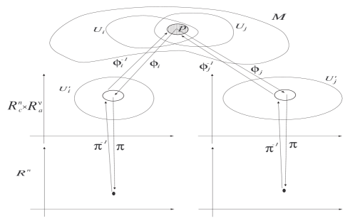
Figure 1: Auræ, as the one shown here (shaded area), are invariant under coordinate transformation: $\phi^{-1}_{i}\circ\pi^{-1}\circ\pi\circ\phi_{i}=\phi^{-1}_{j}\circ\pi^{-1}\circ\pi\circ\phi_{j}$. This enables us to define the body of a supermanifold.

Instead, we have to introduce the term “aura of a point”:

Definition 4.3

Given a supermanifold ${\mathbb{M}}$ with chart $\phi$ mapping ${\mathbb{M}}$ on ${\mathbb{R}}^{n}_{c}\times{\mathbb{R}}^{\nu}_{a}$, then the set $A(x):=\phi^{-1}\circ\pi^{-1}\circ\pi\circ\phi(x)$ for any $x\in{\mathbb{M}}$ is called the aura  of x.

The aura of a point is invariant under coordinate transformation, i.e. $\bar{x}(A(x))=A(\bar{x}(x))$ which is short for

$$\forall p\in A(x):\bar{x}(p)\in A(\bar{x}(x)).$$ (4.4)

Considering auræ as points of a real manifold, we find the invariant definition for the body of a supermanifold:

Definition 4.4

The real manifold ${\mathbb{M}}_{B}=\{A(x)|x\in{\mathbb{M}}\}$ with chart $\pi\circ\phi$ mapping ${\mathbb{M}}$ on ${\mathbb{R}}^{n}$ is called the body of ${\mathbb{M}}$.

In this definition, points of a supermanifold which belong to the same aura are not distinguished. So it is natural to introduce an equivalence class of points:

Definition 4.5

Two points on a supermanifold are called equivalent, if and only if they have the same aura: $x\sim y\Leftrightarrow A(x)=A(y)$.

4.3 Sliced Manifolds

Given a supermanifold ${\mathbb{M}}$ together with the equivalence relation above, we can choose a representative for each equivalence class. Together with the chart $\phi_{S}=\pi\circ\phi$, the set of representatives can be considered as a real manifold $M^{\prime}$. Attaching at each point $p\in{\mathbb{M}}^{\prime}$ all equivalent points $\{p^{\prime}\sim p|p\in{\mathbb{M}}\}$ as a fiber leads to the picture of a sliced manifold ${\mathbb{M}}_{o}$.

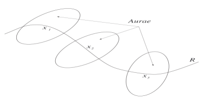
Figure 2: A sliced supermanifold consists of a real manifold $M^{\prime}$, which is the set of chosen representatives for the auræ. The fiber at a point $x$ is the set of equivalent points to the representative $x$: $F_{x}=\{p|p\sim x\}$ and can thus be regarded as the auræ attached to each representative.

Note that given a sliced manifold ${\mathbb{M}}_{o}$ constructed from ${\mathbb{M}}$, each other sliced manifold ${\mathbb{M}}_{o}^{\prime}$ also constructed from ${\mathbb{M}}$ is just a section of ${\mathbb{M}}_{o}$, as it corresponds to a different choice of representatives of the equivalence classes or of elements of the auræ.

A sliced supermanifold is locally described by $n$ real coordinates referring to the body of the supermanifold and $n$ even and $\nu$ odd coordinates, containing Graßmann generators: $(x^{1},...,x^{n},y^{1},...,y^{n},\eta^{1},...,\eta^{\nu})$. The intrinsic coordinate transformation for such a sliced supermanifold is (CT2):

$$\bar{x}^{m} = X^{m}(x)$$ (4.5)

$$\bar{y}^{m} = \sum_{r=0}^{\nu}\sum_{s=0}^{\infty}c_{1}\frac{\partial^{s}Y^{m}_{\mu_{1}...\mu_{r}}(x)}{\partial x^{n_{1}}...\partial x^{n_{s}}}y^{n_{1}}...y_{S}^{n_{s}}\eta^{\mu_{r}}...\eta^{\mu_{1}}$$ (4.6)

$$\bar{\eta}^{\mu} = \sum_{r=0}^{\nu}\sum_{s=0}^{\infty}c_{2}\frac{\partial^{s}Y^{\mu}_{\mu_{1}...\mu_{r}}(x)}{\partial x^{n_{1}}...\partial x^{n_{s}}}y^{n_{1}}...y^{n_{s}}\eta^{\mu_{r}}...\eta^{\mu_{1}}.$$ (4.7)

The constants are the same as in (CT1), $X^{m}(x)$ is an arbitrary bijective function, mapping real numbers to real numbers and $Y^{m}$, $Y^{\mu}$ are functions  ${\mathbb{R}}^{n}\rightarrow{\mathbb{R}}_{c}\backslash{\mathbb{R}}$ or ${\mathbb{R}}^{n}\rightarrow{\mathbb{R}}_{a}$ so that the parity of the equations is matched.

In a further step, we can linearize the slices. It is clear, that varying $(y^{i})_{i}$ and $(\eta^{\iota})_{\iota}$ for one $x$ by bodiless values, we obtain the whole slice at $x$. Since the coordinates are bodiless themselves, multiplication with a supernumber does not change this and we can consider this space as a supervector space over the ring of supernumbers. The intrinsic coordinate transformations here (CT3) are linear maps:

$$\bar{x}^{m} = X^{m}(x)$$ (4.8)

$$\bar{y}^{m} = Y(x)^{m}_{n}y^{n}+Y(x)^{m}_{\nu}\eta^{\nu}$$ (4.9)

$$\bar{\eta}^{\mu} = \Upsilon(x)^{\mu}_{n}y^{n}+\Upsilon(x)^{\mu}_{\nu}\eta^{\nu},$$ (4.10)

where $Y(x)^{m}_{n}$ and $\Upsilon(x)^{\mu}_{\nu}$ are maps ${\mathbb{R}}^{n}\rightarrow{\mathbb{R}}_{c}$ and $Y(x)^{m}_{\nu}$ and $\Upsilon(x)^{\mu}_{n}$ are maps ${\mathbb{R}}^{n}\rightarrow{\mathbb{R}}_{a}$.

4.4 Some sliced manifolds are Kostant manifolds

We use the definition of a Kostant manifold given in Y. Choquet-Bruhat and C. DeWitt-Morette,[7]
A Kostant bundle $K$ over ${\mathbb{M}}$ is a fiber bundle $K$ over a manifold ${\mathbb{M}}$ where the bundle coordinates take their values in a graded algebra $A$ and the transition map from one chart to another commutes with the product of the algebra. Now we can define:

Definition 4.6

A Kostant manifold is a pair $(M,K)$ where ${\mathbb{M}}$ is an ordinary $C^{\infty}$ manifold and $K$ a Kostant bundle over M. A graded function is a section of the bundle.

Let us consider a sliced manifold constructed as above from a supermanifold with dimension $(n,n)$. Locally, we can describe this object by $n$ real variables $x^{i}$, $n$ bodiless even variables $y^{i}$ taking their values in $\Lambda^{\mathrm{even}}$ and $n$ odd variables $\eta^{i}$ with values in $\Lambda^{\mathrm{odd}}$. Since the decomposition of a supernumber in its even and odd parts is unique, we can combine the bodiless coordinates, i.e. the coordinates of the aura, to a new coordinate $z^{i}=y^{i}+\eta^{i}$ without losing any information.

We obtain a real manifold with a bundle, which is a Graßmann algebra without bodiless elements, i.e. generated by the Graßmann generators $\xi^{i}$, but the polynomial of degree zero is not included.

This description of a sliced manifold is obviously also a Kostant manifold. In this sense, B.S. DeWitt’s supermanifolds with equally many odd and even dimensions can always be reduced to Kostant manifolds.

5 Graded manifolds

5.1 Basic definitions

Graded manifolds are the most trivial ones discussed in literature. Their definition is the obvious generalization of real manifolds, using ${\mathbb{R}}^{n|\nu}$ instead of ${\mathbb{R}}$. We follow basically the definition given by Voronov [2].

The space ${\mathbb{R}}^{n|\nu}$ can be defined by the functions on this space which take their values in the Graßmann algebra $\Lambda_{\nu}$:

$$C^{\infty}({\mathbb{R}}^{n|\nu})=\{f_{0}+f_{1}\xi^{1}+...+f_{12}\xi^{1}\xi^{2}+...+f_{1...\nu}\xi^{1}...\xi^{\nu}|f_{I}\in C^{\infty}({\mathbb{R}}^{n})\}$$ (5.1)

It is obvious that ${\mathbb{R}}^{n|\nu}$ can be described by coordinates

$$x^{A}=(x^{a},\xi^{\alpha})=(x^{1},...,x^{n},\xi^{1},...,\xi^{\nu})$$ (5.2)

where the $x^{a}$ and the $\xi^{\alpha}$ are real and Graßmann variables respectively A possible topology of this space is induced by the real component as in the case of supermanifolds. Given the projection $\pi$ by

$$\pi(x^{1},...,x^{n},\xi^{1},...,\xi^{\nu}):=(x^{1},...,x^{n}),$$ (5.3)

a subset $X\subset{\mathbb{R}}^{n|\nu}$ is called open, if and only if $X=\pi^{-1}(Y)$ where $Y$ is an open set in ${\mathbb{R}}^{n}$. As in the case of supermanifolds, with this topology ${\mathbb{R}}^{n|\nu}$ is only projectively hausdorff.

Now we are ready to define:

Definition 5.1

A graded manifold is a topological space which is locally diffeomorphic to ${\mathbb{R}}^{n|\nu}$.

Simple examples for graded manifolds are $\Pi T{\mathbb{M}}$ and $\Pi T^{*}{\mathbb{M}}$, the tangent and cotangent bundle with changed parity of the bundle coordinates.

In the case of graded manifolds, the definition of the body is much easier than for supermanifolds. Here we can use the projection

$$b(x^{1},...,x^{n},\xi^{1},...,\xi^{\nu})=(x^{1},...,x^{n},0,...,0)$$ (5.4)

and the ”naive” definition:

Definition 5.2

Given a graded manifold ${\mathbb{M}}$ then its body ${\mathbb{M}}_{B}$ is given by

$${\mathbb{M}}_{B}=\{b(x)|x\in{\mathbb{M}}\}$$ (5.5)

and its soul is ${\mathbb{M}}_{S}={\mathbb{M}}\backslash{\mathbb{M}}_{B}$.

Since $(\xi^{i})^{2}=0$, we can look at the soul ${\mathbb{M}}_{S}$ of a graded manifold ${\mathbb{M}}$ as infinitely many copies of ${\mathbb{M}}_{B}$ infinitely close to ${\mathbb{M}}_{B}$.

5.2 From supermanifolds to graded manifolds via superfunctions

Though supermanifolds seem to be much richer in their properties than graded manifolds, we are basically interested in the space of functions on both.

On supermanifolds, an arbitrary function can be expanded in polynomials of the odd variables:

$$f(Y,\Upsilon)=f_{0}(Y)+f_{1}(Y)\Upsilon^{1}+...+f_{12}(Y)\Upsilon^{1}\Upsilon^{2}+...+f_{1...\nu}(Y)\Upsilon^{1}...\Upsilon^{\nu}.$$ (5.6)

Here the $f_{I}$ are functions ${\mathbb{R}}_{c}^{n}\rightarrow\Lambda_{\infty}$.

The functions on graded manifolds are, as discussed above:

$$f(x,\xi)=f_{0}(x)+f_{1}(x)\xi^{1}+...+f_{12}(x)\xi^{1}\xi^{2}+...+f_{1...\nu}(x)\xi^{1}...\xi^{\nu},$$ (5.7)

where the $f_{I}$ are functions ${\mathbb{R}}^{n}\rightarrow{\mathbb{R}}$.

With these expansions, it is obvious that functions on supermanifolds and those on graded manifolds differ only in the possible values of the $f_{I}$. As real — or complex — degrees of freedom are sufficient for our purposes, we can constrain our considerations to graded manifolds without fearing to lose properties from supermanifolds.

Part II Integration

6 Definitions and notations

• Forms and densities of weight one on ${\mathbb{M}}^{D}$ (without metric tensor)
  $({\mathcal{A}}^{\bullet}\,,{\mathrm{d}})$ Ascending complex of forms ${\mathrm{d}}:{\mathcal{A}}^{p}\rightarrow{\mathcal{A}}^{p+1}$
  $({\mathcal{D}}_{\bullet}\,,\nabla\cdot\mbox{ or }{\mathrm{b}})$ Descending complex of densities $\nabla\cdot:{\mathcal{D}}_{p}\rightarrow{\mathcal{D}}_{p-1}$
  ${\mathcal{D}}_{p}\equiv{\mathcal{D}}^{-p}$ used for ascending complex in negative degrees

• Operators on ${\mathcal{A}}^{\bullet}({\mathbb{M}}^{D})$
  $M(f):{\mathcal{A}}^{p}\rightarrow{\mathcal{A}}^{p}$, multiplication by a scalar function $f:{\mathbb{M}}^{D}\rightarrow{\mathbb{R}}$
  ${\mathrm{e}}(f):{\mathcal{A}}^{p}\rightarrow{\mathcal{A}}^{p+1}$ by $\omega\mapsto df\wedge\omega$
  ${\mathrm{i}}(X):{\mathcal{A}}^{p}\rightarrow{\mathcal{A}}^{p-1}$ by contraction with the vectorfield $X$
  ${\mathcal{L}}_{X}\equiv{\mathcal{L}}(X)={\mathrm{i}}(X){\mathrm{d}}+{\mathrm{d}}{\mathrm{i}}(X):{\mathcal{A}}^{p}\rightarrow{\mathcal{A}}^{p}$ by the Lie derivative w.r.t. $X$

• Representation of
  fermionic creation operators: ${\mathrm{e}}(x^{m})$
  fermionic annihilation operators: ${\mathrm{i}}(\partial/\partial x^{m})$

• Operators on ${\mathcal{D}}_{\bullet}({\mathbb{M}}^{D})$
  $M(f):{\mathcal{D}}_{p}\rightarrow{\mathcal{D}}_{p}$, multiplication by scalar function $f:{\mathbb{M}}^{D}\rightarrow{\mathbb{R}}$
  ${\mathrm{e}}(f):{\mathcal{D}}_{p}\rightarrow{\mathcal{D}}_{p-1}$ by ${\mathfrak{F}}\mapsto{\mathrm{d}}f.{\mathfrak{F}}$ (contraction with the form ${\mathrm{d}}f$)
  ${\mathrm{i}}(X):{\mathcal{D}}_{p}\rightarrow{\mathcal{D}}_{p+1}$ by multiplication and partial antisymmetrization
  ${\mathcal{L}}_{X}\equiv{\mathcal{L}}(X)={\mathrm{i}}(X){\nabla}+{\nabla}{\mathrm{i}}(X):{\mathcal{D}}_{p}\rightarrow{\mathcal{D}}_{p}$ by Lie derivative w.r.t. $X$

• Forms and densities of weight one on $({\mathbb{M}}^{D}\,,g)$
  $C_{g}:{\mathcal{A}}^{p}\rightarrow{\mathcal{D}}_{p}$ (see eq. 21)
  $\ast:{\mathcal{A}}^{p}\rightarrow{\mathcal{A}}^{D-p}$ s.t ${\mathcal{T}}(\omega|\eta)=\omega\wedge\ast\eta$
  $\delta:{\mathcal{A}}^{p+1}\rightarrow{\mathcal{A}}^{p}$ is the metric transpose defined by
  $~{}~{}~{}~{}~{}~{}[{\mathrm{d}}\omega|\eta]=:[\omega|\delta\eta]$ s.t. $[\omega|\eta]:=\int{\mathcal{T}}(\omega|\eta)$
  $~{}~{}~{}~{}~{}~{}\delta=C_{g}^{-1}bC_{g}~{}~{}~{}~{}~{}~{}~{}~{}~{}~{}~{}\mbox{(see eq. 28)}$
  $\beta:{\mathcal{D}}_{p+1}\rightarrow{\mathcal{D}}_{p}$ is defined by $C_{g}{\mathrm{d}}C_{g}^{-1}$

• Graßmann calculus on $\xi^{\lambda}\in\Lambda_{\nu}$ or $\Lambda_{\infty}$ or unspecified $\Lambda$
  ${\mathrm{d}\mathrm{d}}=0$ remains true, therefore
  $~{}~{}~{}~{}~{}~{}\frac{\partial}{\partial\xi^{\lambda}}\frac{\partial}{\partial\xi^{\mu}}=-\frac{\partial}{\partial\xi^{\mu}}\frac{\partial}{\partial\xi^{\lambda}}$
  $~{}~{}~{}~{}~{}~{}{\mathrm{d}}\xi^{\lambda}\wedge{\mathrm{d}}\xi^{\mu}={\mathrm{d}}\xi^{\mu}\wedge{\mathrm{d}}\xi^{\lambda}$

• Forms and densities of weight $-1$ on ${\mathbb{R}}^{0|\nu}$
  Forms are graded totally symmetric covariant tensors. Densities are graded totally symmetric contravariant tensors of weight -1.
  $\left({\mathcal{A}}^{\bullet}({\mathbb{R}}^{0|\nu})\,,{\mathrm{d}}\right)$ Ascending complex of forms not limited above
  $\left({\mathcal{D}}_{\bullet}({\mathbb{R}}^{0|\nu})\,,\nabla\cdot\mbox{ or }{\mathrm{b}}\right)$ Descending complex of densities not limited above

• Operators on ${\mathcal{A}}^{\bullet}({\mathbb{R}}^{0|\nu})$
  $M(\varphi):{\mathcal{A}}^{p}({\mathbb{R}}^{0|\nu})\rightarrow{\mathcal{A}}^{p}({\mathbb{R}}^{0|\nu})$ multiplication by a scalar function $\varphi$
  ${\mathrm{e}}(\varphi):{\mathcal{A}}^{p}({\mathbb{R}}^{0|\nu})\rightarrow{\mathcal{A}}^{p+1}({\mathbb{R}}^{0|\nu})$ by ${\mathrm{e}}(\varphi)={\mathrm{d}}\varphi\wedge$
  ${\mathrm{i}}(\Xi):{\mathcal{A}}^{p}({\mathbb{R}}^{0|\nu})\rightarrow{\mathcal{A}}^{p-1}({\mathbb{R}}^{0|\nu})$ by contraction with the vectorfield $\Xi$
  ${\mathcal{L}}_{\Xi}\equiv{\mathcal{L}}(\Xi):={\mathrm{i}}(\Xi){\mathrm{d}}-{\mathrm{di}}(\Xi)$ maps ${\mathcal{A}}^{p}({\mathbb{R}}^{0|\nu})\rightarrow{\mathcal{A}}^{p}({\mathbb{R}}^{0|\nu})$

• Representation of
  bosonic creation operators: ${\mathrm{e}}(\xi^{\mu})$
  bosonic annihilation operators: ${\mathrm{i}}(\partial/\partial\xi^{\mu})$

• Operators on ${\mathcal{D}}_{\bullet}({\mathbb{R}}^{0|\nu})$
  $M(\varphi):{\mathcal{D}}_{p}({\mathbb{R}}^{0|\nu})\rightarrow{\mathcal{D}}_{p}({\mathbb{R}}^{0|\nu})$, multiplication by scalar function $\varphi$
  ${\mathrm{e}}(\varphi):{\mathcal{D}}_{p}({\mathbb{R}}^{0|\nu})\rightarrow{\mathcal{D}}_{p-1}({\mathbb{R}}^{0|\nu})$ by ${\mathfrak{F}}\mapsto{\mathrm{d}}(\varphi)\cdot{\mathfrak{F}}$
  ${\mathrm{i}}(\Xi):{\mathcal{D}}_{p}({\mathbb{R}}^{0|\nu})\rightarrow{\mathcal{D}}_{p+1}({\mathbb{R}}^{0|\nu})$ by multiplication and partial symmetrization
  ${\mathcal{L}}_{\Xi}\equiv{\mathcal{L}}(\Xi)={\mathrm{i}}(\Xi){\nabla}-{\nabla}{\mathrm{i}}(\Xi):{\mathcal{D}}_{p}({\mathbb{R}}^{0|\nu})\rightarrow{\mathcal{D}}_{p}({\mathbb{R}}^{0|\nu})$ by Lie derivative w.r.t. $\Xi$

7 Recalling classical results

7.1 Forms and densities on a $D$-dimensional manifold

We single out the statements which are independent of the dimension $D$ of the manifold because our ultimate goal is integration on infinite dimensional spaces.

We begin with properties of forms and densities which can be established in the absence of a metric tensor because they are readily useful in Graßmann calculus; we then consider forms and densities on riemannian manifolds $({\mathbb{M}}^{D}\,,g)$.

By “forms” we mean exterior differential forms, i.e. totally antisymmetric covariant tensors.

By “densities” we mean tensor-densities of weight one, i.e. totally antisymmetric contravariant tensors of weight one. A density ${\mathfrak{F}}$ is said to be of weight $w$ if, under the change of coordinate $\bar{x}(x)$, the new density $\bar{\mathfrak{F}}$ is proportional to $(\det\partial\bar{x}/\partial x)^{w}$.

7.2 Forms

The exterior differentiation ${\mathrm{d}}$ on the graded algebra ${\mathcal{A}}^{\bullet}$ of forms is a derivation  of degree 1. Let ${\mathcal{A}}^{p}$ be the space of $p$-forms on ${\mathbb{M}}^{D}$,

$${\mathrm{d}}:{\mathcal{A}}^{p}\longrightarrow{\mathcal{A}}^{p+1}$$ (7.1)

In coordinates, using the convention that capitalized indices are ordered,

$${\mathrm{d}}\omega = \frac{\partial\omega_{I_{1}\ldots I_{p}}}{\partial x^{m}}{\mathrm{d}}x^{m}\wedge{\mathrm{d}}x^{I_{1}}\wedge\ldots\wedge{\mathrm{d}}x^{I_{p}}$$

$$= \varepsilon\begin{array}[]{l}mI_{1}\ldots I_{p}\\[-1.4457pt] J_{1}\ldots J_{p+1}\end{array}\frac{\partial\omega_{I_{1}\ldots I_{p}}}{\partial x^{m}}{\mathrm{d}}x^{J_{1}}\wedge\ldots\wedge{\mathrm{d}}x^{J_{p+1}}$$

$$= \frac{1}{(p+1)!}\theta_{j_{1}\ldots j_{p+1}}{\mathrm{d}}x^{j_{1}}\wedge\ldots\wedge{\mathrm{d}}x^{j_{p+1}}$$

which defines the components of $\theta={\mathrm{d}}\omega$. We recall the following operators on ${\mathcal{A}}^{\bullet}$ and some of their properties

$$\begin{array}[]{lcll}M(f)&:&{\mathcal{A}}^{j}\longrightarrow{\mathcal{A}}^{j}&\mbox{by multiplication with }f:{\mathbb{M}}^{D}\rightarrow{\mathbb{R}}\\ {\mathrm{e}}(f)&:&{\mathcal{A}}^{j}\longrightarrow{\mathcal{A}}^{j+1}&\mbox{by }\omega\mapsto df\wedge\omega\\ {\mathrm{i}}(X)&:&{\mathcal{A}}^{j}\longrightarrow{\mathcal{A}}^{j-1}&\mbox{by contraction with the vector }X\\ {\mathcal{L}}_{X}\equiv{\mathcal{L}}(X)&:&{\mathcal{A}}^{j}\longrightarrow{\mathcal{A}}^{j}&\mbox{by the Lie derivative w.r.t. }X\end{array}$$ (7.5)

Their graded commutators are

$$\left[{\mathrm{e}}(f)\,,{\mathrm{e}}(g)\right]_{+}=0$$ (7.6)

$$\left[{\mathrm{i}}(X)\,,{\mathrm{i}}(Y)\right]_{+}=0$$ (7.7)

$$\left[{\mathrm{i}}(X)\,,{\mathrm{e}}(f)\right]_{+}=M({\mathcal{L}}_{X}f)$$ (7.8)

With respect to the exterior differential ${\mathrm{d}}$ we have the following graded commutators

$$\left[{\mathrm{d}}\,,{\mathrm{e}}(f)\right]_{+} = 0$$ (7.9)

$$\left[{\mathrm{d}}\,,{\mathrm{i}}(X)\right]_{+} = {\mathcal{L}}_{X}$$ (7.10)

$$\left[{\mathrm{d}}\,,{\mathcal{L}}_{X}\right]_{-} = 0$$ (7.11)

which may be obtained from the explicit representation

$${\mathrm{d}}={\mathrm{e}}(x^{m}){\mathcal{L}}(\partial/\partial x^{m})\,.$$ (7.12)

Interpreting the degree $p$ of a form as a particle number, we note that ${\mathrm{e}}(x^{m})$ is a fermionic creation operator and ${\mathrm{i}}(\partial/\partial x^{m})$ is a fermionic annihilation operator.

7.3 Densities

A $p$-density is a density whose contraction with a $p$-form is a scalar-density. In the coordinate basis $(\partial/\partial x^{j})_{j}$ dual to $({\mathrm{d}}x^{j})_{j}$ and using capitalized (ordered) indices

$${\mathfrak{F}}=\sqrt{{\mathrm{det}}\,g}\frac{\partial}{\partial x^{I_{1}}}\wedge...\wedge\frac{\partial}{\partial x^{I_{p}}}{\mathfrak{F}}^{I_{1}...I_{p}}$$ (7.13)

A scalar density is simply ${\mathfrak{F}}$.

Let ${\mathcal{D}}_{p}$ be the space of $p$-densities , the divergence operator

$$\nabla\cdot:{\mathcal{D}}_{p}\longrightarrow{\mathcal{D}}_{p-1}\,.$$ (7.14)

In coordinates

$$(\nabla\cdot{\mathfrak{F}})^{\nu\ldots}=\frac{\partial}{\partial x^{\mu}}{\mathfrak{F}}^{\mu\nu\ldots}$$ (7.15)

To conform with standard practice for descending complexes, we shall write the divergence operation $\nabla\cdot$ on densities also as ${\mathrm{b}}$ (for boundary) typically using ${\mathrm{b}}$ in the context of complexes and $\nabla$ in the context of computation.[6] We introduce the following operators on ${\mathcal{D}}_{\bullet}$

$$\begin{array}[]{ll}M(f):{\mathcal{D}}_{p}\longrightarrow{\mathcal{D}}_{p}&\mbox{by multiplication with }f:{\mathbb{M}}^{D}\rightarrow{\mathbb{R}}\\ {\mathrm{e}}(f):{\mathcal{D}}_{p}\longrightarrow{\mathcal{D}}_{p-1}&\mbox{by contraction with }{\mathrm{d}}(f)\\ {\mathrm{i}}(X):{\mathcal{D}}_{p}\longrightarrow{\mathcal{D}}_{p+1}&\mbox{by multiplication and }\\ &\mbox{partial antisymmetrization}\\ {\mathcal{L}}_{X}\equiv{\mathcal{L}}(X):{\mathcal{D}}_{p}\longrightarrow{\mathcal{D}}_{p}&\mbox{by the Lie derivative w.r.t. }X\end{array}$$ (7.16)

Example: Let ${\mathfrak{F}}$ be a 2-density, then

$$\left({\mathrm{i}}(X){\mathfrak{F}}\right)^{\alpha\beta\gamma}=X^{\alpha}{\mathfrak{F}}^{\beta\gamma}+X^{\beta}{\mathfrak{F}}^{\gamma\alpha}+X^{\gamma}{\mathfrak{F}}^{\alpha\beta}\,.$$ (7.17)

As in the case of forms, we obtain the commutator relations:

$$[{\mathrm{e}}(f)\,,{\mathrm{e}}(g)]_{+}=0$$ (7.18)

$$[{\mathrm{i}}(X)\,,{\mathrm{i}}(Y)]_{+}=0$$ (7.19)

$$[{\mathrm{e}}(f)\,,{\mathrm{i}}(X)]_{+}=M({\mathcal{L}}_{X}f)$$ (7.20)

and

$$[\nabla\,,{\mathrm{e}}(f)]_{+}=0$$ (7.21)

$$[\nabla\,,{\mathrm{i}}(X)]_{+}=\frac{\partial}{\partial x^{\mu}}X^{\mu}$$ (7.22)

$$[\nabla\,,{\mathcal{L}}_{X}]_{-}=0.$$ (7.23)

which may be obtained from the explicit representation 

$$\nabla={\mathrm{e}}(x^{m}){\mathcal{L}}(\partial/\partial x^{m}).$$ (7.24)

Interpreting the degree $p$ of a density as a particle number (i.e. the sum of all occupation numbers), we note that ${\mathrm{e}}(x^{m})$ is a fermionic annihilation operator and ${\mathrm{i}}(\partial/\partial x^{m})$ is a fermionic creation operator.

7.4 Ascending and descending complexes on ${\mathbb{M}}^{D}$

Since ${\mathrm{d}}{\mathrm{d}}=0$, the graded algebra ${\mathcal{A}}^{\bullet}$ is an ascending complex w.r.t. to the operator ${\mathrm{d}}$

$${\mathcal{A}}^{0}\stackrel{{\scriptstyle{\mathrm{d}}}}{{\longrightarrow}}{\mathcal{A}}^{1}\longrightarrow\cdots\longrightarrow{\mathcal{A}}^{D}\,.$$ (7.25)

Since ${\mathrm{b}}{\mathrm{b}}=0$, the following sequence is a descending complex.

$${\mathcal{D}}_{0}\stackrel{{\scriptstyle\mathrm{b}}}{{\longleftarrow}}{\mathcal{D}}_{1}\stackrel{{\scriptstyle\mathrm{b}}}{{\longleftarrow}}\cdots\longleftarrow{\mathcal{D}}_{D-1}\stackrel{{\scriptstyle\mathrm{b}}}{{\longleftarrow}}{\mathcal{D}}_{D}$$ (7.26)

Writing ${\mathcal{D}}^{-p}$ instead of ${\mathcal{D}}_{p}$ is standard practise in homological algebra, and the descending complex can be written as an ascending complex in negative degrees

$${\mathcal{D}}^{-D}\stackrel{{\scriptstyle\mathrm{b}}}{{\longrightarrow}}{\mathcal{D}}^{-D+1}\stackrel{{\scriptstyle\mathrm{b}}}{{\longrightarrow}}\cdots\longrightarrow{\mathcal{D}}^{-1}\stackrel{{\scriptstyle\mathrm{b}}}{{\longrightarrow}}{\mathcal{D}}^{0}\,.$$ (7.27)

Remark: The operator ${\mathrm{i}}(X)$ moves downwards on the ascending complex ${\mathcal{A}}^{\bullet}$, and upwards on the descending complex ${\mathcal{D}}_{\bullet}$.

7.5 Forms and densities on a riemannian manifold $({\mathbb{M}}^{D}\,,g)$

The metric tensor $g$ provides a correspondence $C_{g}$ between a $p$-form and a $p$-density. For instance, let $F$ by a 2 form, then

$${\mathfrak{F}}^{\alpha\beta}=\sqrt{\det g_{\mu\nu}}F_{\gamma\delta}g^{\alpha\gamma}g^{\beta\delta}$$ (7.28)

are components of a 2-density. The metric $g$ is used twice: a) raising indices, b) introducing weight 1 by multiplication with $\sqrt{\det g}$. This correspondence does not depend on the dimension $D$.

On an orientable manifold, the dimension $D$ can be used for transforming a $p$-density into a $(D-p)$-form. For example let $D=4$ and $p=1$

$$t_{\alpha\beta\gamma}:=\varepsilon^{1234}_{\alpha\beta\gamma\delta}{\mathfrak{F}}^{\delta}$$ (7.29)

where the alternating symbol $\varepsilon$ defines an orientation.

The star operator (Hodge-de Rham operator, see Ref.  [7], p. 295)) combines the metric-dependent and the dimension-dependent transformations; it transforms a $p$-form into a $(D-p)$-form by

$${\mathcal{T}}(\omega|\eta)=\omega\wedge\ast\eta$$ (7.30)

where, as usual, the scalar product of 2 $p$-form $\omega$ and $\eta$ is

$$(\omega|\eta)=\frac{1}{p!}\omega_{i_{1}\ldots i_{p}}\eta^{i_{1}\ldots i_{p}}$$ (7.31)

and ${\mathcal{T}}$ is the volume element, given in example 1 below.

We shall exploit the correspondence mentioned in the first paragraph

$$C_{g}:{\mathcal{A}}^{p}\longrightarrow{\mathcal{D}}_{p}$$ (7.32)

for constructing a descending complex on ${\mathcal{A}}^{\bullet}$ w.r.t. to the metric transpose $\delta$ of $\mathrm{d}$ (Ref.  [7], p. 296)

$$\delta:{\mathcal{A}}^{p+1}\longrightarrow{\mathcal{A}}^{p}$$ (7.33)

and an ascending complex on ${\mathcal{D}}_{\bullet}$

$$\beta:{\mathcal{D}}_{p}\longrightarrow{\mathcal{D}}_{p+1}$$ (7.34)

where $\beta$ is defined by the following diagram

$$\left.\begin{array}[]{clclc}{}\hfil&{\mathcal{A}}^{p}&\begin{array}[]{c}\stackrel{{\scriptstyle\scriptstyle{\delta}}}{{\textstyle{\longleftarrow}}}\\[-3.61371pt] \stackrel{{\scriptstyle\textstyle{\longrightarrow}}}{{\scriptstyle{d}}}\end{array}&{\mathcal{A}}^{p+1}&{}\hfil\\[-3.61371pt] C_{g}&\downarrow&{}\hfil&\downarrow&C_{g}\\[-3.61371pt] {}\hfil&{\mathcal{D}}_{p}&\begin{array}[]{c}\stackrel{{\scriptstyle\beta}}{{\longrightarrow}}\\[-3.61371pt] \stackrel{{\scriptstyle\textstyle{\longleftarrow}}}{{\scriptstyle{b}}}\end{array}&{\mathcal{D}}_{p+1}&{}\hfil\end{array}\right\}\Longleftrightarrow\left\{\begin{array}[]{rcl}\delta&=&C^{-1}_{g}bC_{g}\\[8.67204pt] \beta&=&C_{g}dC^{-1}_{g}\end{array}\right.\,.$$ (7.35)

Example 1: Volume element on an oriented $D$-dimensional riemannian manifold. The volume element is

$${\mathcal{T}}:={\mathrm{d}}x^{1}\wedge\ldots\wedge{\mathrm{d}}x^{D}\,{\mathfrak{T}}=~{}{\mathrm{d}}x^{1}\wedge\ldots\wedge{\mathrm{d}}x^{D}\,\sqrt{\det g}\mbox{ with }{\mathfrak{T}}\in{\mathcal{D}}_{0}$$ (7.36)

where ${\mathfrak{T}}$ is a scalar density corresponding to the top form

$${\mathrm{d}}x^{1}\wedge\ldots\wedge{\mathrm{d}}x^{D}\in{\mathcal{A}}^{D}$$ (7.37)

${\mathfrak{T}}$ is indeed a scalar density since, under the change of coordinates $x^{\prime j}=A^{j}{}_{i}x^{i}$

$${\mathfrak{T}}^{\prime}=(\det A){\mathfrak{T}}\,.$$ (7.38)

Example 2: In the thirties, the use of densities was often justified by the fact that in a number of useful examples it reduces the number of indices. For example, a vector-density in ${\mathbb{M}}^{4}$ can replace a 3-form

$${\mathfrak{T}}^{l}=\sqrt{\det g}~{}\varepsilon^{ijkl}_{1234}t_{ijk}\,.$$ (7.39)

An axial vector in ${\mathbb{R}}^{3}$ can replace a 2-form.

7.6 Other definitions of the metric transpose $\delta$ .

• The name “metric transpose of the differential ${\mathrm{d}}$” comes from the integrated version of ${\mathcal{T}}(\omega|\eta)=\omega\wedge\ast\eta$; namely let

  $$[\omega|\eta]=\int{\mathcal{T}}(\omega|\eta)$$ (7.40)

  then for $\omega$ a $p$-form and $\eta$ a $(p+1)$-form on a manifold without boundary $\delta$ is defined by

  $$[{\mathrm{d}}\omega|\eta]=:[\omega|\delta\eta]\,.$$ (7.41)

• On a $p$-form $\omega$,

  $$\delta\omega:=(-1)^{p}\ast^{-1}{\mathrm{d}}\ast\omega$$ (7.42)

  where $\ast$ is the star operator defined above.

• $\delta$ is a derivation on ${\mathcal{A}}^{\bullet}$ of degree -1.

We have given a new presentation of these well known results, but we have separated metric-dependent and dimension-dependent transformations. It brings forth the ascending complex on densities w.r.t. to the operator $\beta=C_{g}{\mathrm{d}}C_{g}^{-1}$.

8 Berezin integration

8.1 A Berezin integral is a derivation

The fundamental requirement on a definite integral is expressed in terms of an integral operator $I$ and a derivative operator $D$ on a space of functions, namely

$$DI=ID=0$$ (8.1)

The requirement $DI=0$ for functions of real variables $f:{\mathbb{R}}^{D}\longrightarrow{\mathbb{R}}$ says that the integral does not depend on the variable of integration

$$\frac{{\mathrm{d}}}{{\mathrm{d}}x}\int f(x){\mathrm{d}}x=0\,,\qquad x\in{\mathbb{R}}\,.$$ (8.2)

The requirement $ID=0$ on the space of functions defined on domains with vanishing boundaries says

$$\int\frac{{\mathrm{d}}}{{\mathrm{d}}x}f(x){\mathrm{d}}x=0$$ (8.3)

This is the foundation of integration by parts

$$0=\int{\mathrm{d}}\left(f(x)g(x)\right)=\int{\mathrm{d}}f(x)\cdot g(x)+\int f(x){\mathrm{d}}g(x)\,,$$ (8.4)

and of the Stokes’ theorem on a form $\omega$,

$$\int_{\mathbb{M}}{\mathrm{d}}\omega=\int_{\partial\mathbb{M}}\omega=0\qquad\mbox{since }\partial\mathbb{M}\mbox{ is an empty set}$$ (8.5)

We shall use the requirement $ID=0$ in section II.5 for imposing a condition on volume elements.

We now use the fundamental requirements on Berezin integrals defined on functions $f$ of the Grassman algebra $\Lambda_{\nu}$. The condition $DI=0$ says

$$\frac{\partial}{\partial\xi^{i}}I(f)=0\qquad\qquad\mbox{for }i\in\{1\,,\ldots\,,\nu\}$$ (8.6)

Any operator on $\Lambda_{\nu}$ can be set in normal ordering 

$$\Sigma C_{K}{}^{J}\xi^{K}\frac{\partial}{\partial\xi^{J}}$$ (8.7)

with $J\,,K\,,$ multi-ordered indices. Therefore the condition $DI=0$ implies that $I$ is a polynomial in $\partial/\partial\xi^{i}$,

$$I=Q\left(\frac{\partial}{\partial\xi^{1}}\,,\ldots\frac{\partial}{\partial\xi^{\nu}}\right)\,.$$ (8.8)

The condition $ID=0$, namely

$$Q\left(\frac{\partial}{\partial\xi^{1}}\,,\ldots\,,\frac{\partial}{\xi^{\nu}}\right)\frac{\partial}{\partial\xi^{\mu}}=0\qquad\mbox{for every }i\in\{1\,,\ldots\,,\nu\}\,,$$ (8.9)

implies

$$I=\mbox{constant }\frac{\partial}{\partial\xi^{\nu}}\cdots\frac{\partial}{\partial\xi^{1}}$$ (8.10)

A Berezin integral is a derivation. The constant is a normalisation constant chosen for convenience in the given context. Usual choices include $1$, $(2\pi i)^{1/2}$, $(2\pi i)^{-1/2}$.

8.2 Change of variable of integration

Since integrating $f(\xi^{1}\,,\ldots\,,\xi^{\nu})$ is taking its derivatives w.r.t. $\xi^{1}\,,\ldots\,,\xi^{\nu}$, a change of variable of integration is most easily performed on the derivatives. Given a change of coordinates $f$, we recall the induced transformations on the tangent and cotangent spaces. Let $y=f(x)$ and $\theta=f(\zeta)$;

$${\mathrm{d}}y^{1}\wedge\ldots\wedge{\mathrm{d}}y^{D}={\mathrm{d}}x^{1}\wedge\ldots\wedge{\mathrm{d}}x^{D}\left(\det\frac{\partial y^{i}}{\partial x^{j}}\right)$$ (8.11)

and

$$\int{\mathrm{d}}x^{1}\wedge\ldots\wedge{\mathrm{d}}x^{D}\,(F\circ f)(x)\left(\det\frac{\partial f^{i}}{\partial x^{j}}\right)=\int{\mathrm{d}}y^{1}\wedge\ldots\wedge{\mathrm{d}}y^{D}\,F(y)$$ (8.12)

On the other hand, for an intregral over Graßmann variables, the antisymmetry leading to a determinant is the antisymmetry of the product $\partial_{1}\ldots\partial_{D}$. And

$$\left(\frac{\partial}{\partial\zeta^{1}}\ldots\frac{\partial}{\partial\zeta^{D}}\right)(F\circ f)(\zeta)=\left(\det\frac{\partial\theta^{\lambda}}{\partial\zeta^{\mu}}\right)\frac{\partial}{\partial\theta^{1}}\cdots\frac{\partial}{\partial\theta^{D}}F(\theta)$$ (8.13)

The determinant is now on the right hand side, it will become an inverse determinant when brought to the same side as in (8.12).

9 Ascending and descending complexes in Graßmann calculus

In section 7.5 we have presented ${\mathrm{d}}$-ascending and $\delta$-descending complexes ${\mathcal{A}}^{\bullet}({\mathbb{M}})$ of forms and ${\mathrm{b}}$-descending and $\beta$-ascending complexes ${\mathcal{D}}_{\bullet}({\mathbb{M}})$ of densities. We shall now study complexes ${\mathcal{A}}^{\bullet}({\mathbb{R}}^{0|\nu})$ of Graßmann forms, and complexes ${\mathcal{D}}_{\bullet}({\mathbb{R}}^{0|\nu})$ of Graßmann densities.

9.1 Graßmann Forms

Two properties of forms on real variables remain true for forms on Graßmann variables, namely

$${\mathrm{d}}{\mathrm{d}}\omega=0$$ (9.1)

$${\mathrm{d}}(\omega\wedge\theta)={\mathrm{d}}\omega\wedge\theta+(-1)^{\tilde{\omega}\tilde{d}}\omega\wedge d\theta\,;$$ (9.2)

a form on Graßmann variables is a graded totally antisymmetric covariant tensor. Indeed

$$\xi^{\lambda}\xi^{\mu}=-\xi^{\mu}\xi^{\lambda}$$ (9.3)

implies

$$\partial_{\lambda}\partial_{\mu}=-\partial_{\mu}\partial_{\lambda}\qquad\qquad\mbox{where}\qquad\partial_{\lambda}:=\partial/\partial\xi^{\lambda}$$ (9.4)

which, in turn implies

$$d\xi^{\lambda}\wedge d\xi^{\mu}=d\xi^{\mu}\wedge d\xi^{\lambda}.$$ (9.5)

The counterparts on ${\mathcal{A}}^{\bullet}({\mathbb{R}}^{0|\nu})$ of the operators $M(f)$, ${\mathrm{e}}(f)$, ${\mathrm{i}}(X)$, ${\mathcal{L}}(X)$ on ${\mathcal{A}}^{\bullet}({\mathbb{M}})$ are as follows; we omit the reference to ${\mathbb{R}}^{0|\nu}$ for visual clarity.

$$\begin{array}[]{rcll}M(\varphi)&:&{\mathcal{A}}^{j}\longrightarrow{\mathcal{A}}^{j}&~{}~{}~{}~{}\mbox{by multiplication by }\varphi:{\mathbb{R}}^{0|\nu}\rightarrow\Lambda_{\nu}\\ {\mathrm{e}}(\varphi)&:&{\mathcal{A}}^{j}\longrightarrow{\mathcal{A}}^{j+1}&~{}~{}~{}~{}\mbox{by }{\mathrm{e}}(\varphi):={\mathrm{d}}\varphi\wedge\\ {\mathrm{i}}(\Xi)&:&{\mathcal{A}}^{j}\longrightarrow{\mathcal{A}}^{j-1}&~{}~{}~{}~{}\mbox{by contraction with }\Xi\\ {\mathcal{L}}_{\Xi}\equiv{\mathcal{L}}(\Xi)&:&{\mathcal{A}}^{j}\longrightarrow{\mathcal{A}}^{j}&~{}~{}~{}~{}\mbox{by Lie derivative with respect to }\Xi\end{array}$$ (9.6)

We note the following properties 

$${\mathrm{i}}(\Xi)(\omega^{k}\wedge\eta)=\left({\mathrm{i}}(\Xi)\omega^{k}\right)\wedge\eta+\omega^{k}\wedge{\mathrm{i}}(\Xi)\eta\qquad\omega^{k}\in{\mathcal{A}}^{k}$$ (9.7)

i.e. the parity of ${\mathrm{i}}(\Xi)$ is zero. It follows that

$${\mathcal{L}}(\Xi)={\mathrm{i}}(\Xi)d-d{\mathrm{i}}(\Xi)$$ (9.8)

For $\varphi$, $\xi$, $\Xi$, $\Psi$ odd, the corresponding graded commutators are

$$\left[{\mathrm{e}}(\varphi)\,,{\mathrm{e}}(\zeta)\right]_{-} = 0$$ (9.9)

$$\left[{\mathrm{i}}(\Xi)\,,{\mathrm{i}}(\Psi)\right]_{-} = 0$$ (9.10)

$$\left[{\mathrm{i}}(\Xi)\,,{\mathrm{e}}(\varphi)\right]_{-} = M({\mathcal{L}}_{\Xi}\varphi)$$ (9.11)

$$\left[{\mathrm{d}}\,,{\mathrm{e}}(\varphi)\right]_{-} = 0$$ (9.12)

$$\left[{\mathrm{d}}\,,{\mathrm{i}}(\Xi)\right]_{-} = {\mathcal{L}}_{\Xi}$$ (9.13)

$$\left[{\mathrm{d}}\,,{\mathcal{L}}(\Xi)\right]_{+} = 0$$ (9.14)

which may be obtained from the explicit representation

$${\mathrm{d}}={\mathrm{e}}(\xi^{\mu}){\mathcal{L}}\left(\partial/\partial\xi^{\mu}\right)$$ (9.15)

Interpreting the degree $p$ of a Graßmann form as a particle number, we note that ${\mathrm{e}}(\xi^{\mu})$ is a bosonic creation operator and ${\mathrm{i}}(\partial/\partial\xi^{\mu})$ is a bosonic annihilation operator.

Since the differential of a Graßmann variable has even parity (9.5), there is at first no reason to restrict our forms to polynomials in $\mathrm{{\mathrm{d}}}\xi^{i}$. (The space of polynomials is a proper subset of the space of smooth functions.) This leads to arbitrary smooth functions $\omega=\omega(\xi^{i},\mathrm{{\mathrm{d}}}\xi^{i})$, which Voronov [2] calls pseudodifferential forms. Those forms can obviously no longer be decomposed in even and odd parts. Since we consider this necessary for the description of the quantum Fock space, we restrict our considerations to polynomial forms.

9.2 Graßmann Densities

In order to define Graßmann densities we recall the definitions of densities in the works of H. Weyl [8] (1920) W. Pauli [9] (1921) and L. Brillouin [10] (1938). From Pauli’s Theory of Relativity (p. 32): “If the integral $\int{\mathfrak{F}}{\mathrm{d}}x$ is an invariant (in a change of coordinate system), then ${\mathfrak{F}}$ is called a scalar density, following Weyl’s terminology” (in Space-Time-Matter pp 109 ff). Here ${\mathrm{d}}x$ stands for ${\mathrm{d}}x^{1}\wedge\ldots\wedge{\mathrm{d}}x^{D}$. Under the change of variable $y(x)$, ${\mathfrak{F}}$ is a scalar density if it is a scalar multiplied by $\det(\partial y^{j}/\partial x^{i})$.

What we call here “tensor-densities” is called “linear tensor densities” by Weyl. For him the term “tensor densities” are arbitrary tensors of weight one. He singles out among them the contravariant antisymmetric  ones and calls them “linear” because, like the “covariant skew-symmetrical tensors” (i.e. the forms), they play a “unique part.” Their unique properties, algebraic and geometrical are beautifully presented in Brillouin’s book. Brillouin defines “capacity” as an object which multiplied by a density is a scalar. Together densities and capacities have become known as “pseudo-tensors” and are sometimes treated as “second rate” tensors!

If the Berezin integral $\int{\mathrm{d}}\xi^{\nu}...{\mathrm{d}}\xi^{1}\,f(\xi^{1},\ldots,\xi^{\nu})=\frac{\partial}{\partial\xi^{\nu}}\cdots\frac{\partial}{\partial\xi^{1}}f(\xi^{1},\ldots,\xi^{\nu})$ is invariant under the change of coordinates $\theta(\xi)$ then $f$ is a Graßmann scalar density. It follows from the formula for change of variable of integration (8.13) that a Graßmann scalar density is a scalar divided by $\det\left(\partial\theta^{\lambda}/\partial\xi^{\mu}\right)$. The expression $\frac{\partial}{\partial\xi^{\nu}}\cdots\frac{\partial}{\partial\xi^{1}}$ is a Graßmann capacity in ${\mathbb{R}}^{0|\nu}$.

Two properties of densities on real variables remain true for Graßmann densities ${\mathfrak{F}}$, namely

$$(\nabla\cdot)(\nabla\cdot){\mathfrak{F}}=0$$ (9.16)

$$(\nabla\cdot)(X{\mathfrak{F}})=(\nabla\cdot X)\cdot{\mathfrak{F}}+(-1)^{\tilde{X}\tilde{\nabla}}X\nabla\cdot{\mathfrak{F}}$$ (9.17)

where $X$ is a vector field. The first property follows from the fact that the Graßmann divergence is odd and the density is a graded antisymmetric contraviant tensor, i.e. symmetric in the interchange of two Graßmann indices.

The second property is the “Leibnitz” property of divergence over products. A density is a tensor of weight 1; multiplication by a tensor of weight zero is the only possible product which maps a density into a density.

Together these two properties make possible the construction of a density complex.

Multiplying a Graßmann scalar density ${\mathfrak{F}}$ by a graded totally antisymmetric contravariant tensor gives a Graßmann tensor density of components

$${\mathfrak{F}}^{\mu\nu\rho\ldots}$$ (9.18)

The counterparts on ${\mathcal{D}}_{\bullet}({\mathbb{R}}^{0|\nu})$ of the operators $M(f)$, ${\mathrm{e}}(f)$, ${\mathrm{i}}(X)$, ${\mathcal{L}}(X)$ on ${\mathcal{D}}_{\bullet}({\mathbb{M}})$ are as follows. We omit the reference to ${\mathbb{R}}^{0|\nu}$ for visual clarity.

$$\begin{array}[]{ll}M(\varphi):{\mathcal{D}}_{p}\longrightarrow{\mathcal{D}}_{p}{}{}&~{}~{}\mbox{by multiplication by }\varphi:{\mathbb{R}}^{0|\nu}\longrightarrow{\mathbb{R}}\\ {\mathrm{e}}(\varphi):{\mathcal{D}}_{p}\longrightarrow{\mathcal{D}}_{p-1}{}{}&~{}~{}\mbox{by contraction with }{\mathrm{d}}(\varphi)\\ {\mathrm{i}}(\Xi):{\mathcal{D}}_{p}\longrightarrow{\mathcal{D}}_{p+1}{}{}&~{}~{}\mbox{by multiplication and}\\ &~{}~{}\mbox{partial antisymmetrization}\\ {\mathcal{L}}_{\Xi}\equiv{\mathcal{L}}(\Xi):{\mathcal{D}}_{p}\longrightarrow{\mathcal{D}}_{p}{}{}&~{}~{}\mbox{by the Lie derivative w.r.t. }\Xi\end{array}$$ (9.19)

9.3 Ascending and descending Graßmann complexes

The ascending complex ${\mathcal{A}}^{\bullet}({\mathbb{R}}^{0|\nu})$ of Graßmann forms with respect to ${\mathrm{d}}$ does not terminate at the $\nu$-form. The descending complex ${\mathcal{D}}_{\bullet}({\mathbb{R}}^{0|\nu})$ of densities with respect to $\nabla$ does not terminate at the $\nu$-density. Indeed, whereas forms and densities on ordinary variables are antisymmetric tensors, on Graßmann variables they are symmetric tensors, therefore their degrees are not limited to the Graßmann dimension $\nu$.

9.4 Summary of complexes on ordinary and Graßmann variables

On ${\mathbb{M}}^{D}$:

$${\mathcal{D}}_{D}\longrightarrow\phantom{{\mathcal{D}}_{1}\longrightarrow} ... \longrightarrow{\mathcal{D}}_{0}\,$$ (9.20)

$${\mathcal{A}}^{0}\,\stackrel{{\scriptstyle{\mathrm{d}}}}{{\longrightarrow}}{\mathcal{A}}^{1}\stackrel{{\scriptstyle{\mathrm{d}}}}{{\longrightarrow}} ... \stackrel{{\scriptstyle{\mathrm{d}}}}{{\longrightarrow}}{\mathcal{A}}^{D}$$ (9.21)

$${\mathcal{D}}_{0}\,\stackrel{{\scriptstyle\mathrm{b}}}{{\longleftarrow}}{\mathcal{D}}_{1}\stackrel{{\scriptstyle\mathrm{b}}}{{\longleftarrow}} ... \stackrel{{\scriptstyle\mathrm{b}}}{{\longleftarrow}}{\mathcal{D}}_{D}$$ (9.22)

${\mathcal{D}}_{0}\rightarrow{\mathcal{A}}^{D}$ by a dimension-dependent equation (a scalar density is the strict component of a top form)
${\mathcal{A}}^{0}\rightarrow{\mathcal{D}}_{0}$ by a metric-dependent equation.

• on ${\mathcal{A}}^{\bullet}({\mathbb{M}}^{D})$, ${\mathrm{e}}(x^{k})$ represents a fermionic creation operator ${\mathrm{i}}(\partial/\partial x^{k})$ represents a fermionic annihilation operator.

• on ${\mathcal{D}}_{\bullet}({\mathbb{M}}^{D})$, ${\mathrm{e}}(x^{k})$ represents a fermionic annihilation operator ${\mathrm{i}}(\partial/\partial x^{k})$ represents a fermionic creation operator.

On ${\mathbb{R}}^{0|\nu}$:

$$...{\mathcal{D}}_{\nu}\longrightarrow\phantom{{\mathcal{D}}_{1}\longrightarrow} ... \longrightarrow{\mathcal{D}}_{0}$$ (9.23)

$$\phantom{...}{\mathcal{A}}^{0}\,\stackrel{{\scriptstyle{\mathrm{d}}}}{{\longrightarrow}}{\mathcal{A}}^{1}\stackrel{{\scriptstyle{\mathrm{d}}}}{{\longrightarrow}} ... \stackrel{{\scriptstyle{\mathrm{d}}}}{{\longrightarrow}}{\mathcal{A}}^{\nu}...$$ (9.24)

$$\phantom{...}{\mathcal{D}}_{0}\,\stackrel{{\scriptstyle\mathrm{b}}}{{\longleftarrow}}{\mathcal{D}}_{1}\stackrel{{\scriptstyle\mathrm{b}}}{{\longleftarrow}} ... \stackrel{{\scriptstyle\mathrm{b}}}{{\longleftarrow}}{\mathcal{D}}_{\nu}...$$ (9.25)

• on ${\mathcal{A}}^{\bullet}({\mathbb{R}}^{0|\nu})$, ${\mathrm{e}}(\xi^{\mu})$ represents a bosonic creation operator ${\mathrm{i}}(\partial/\partial\xi^{\mu})$ represents a bosonic annihilation operator.

• on ${\mathcal{D}}_{\bullet}({\mathbb{R}}^{0|\nu})$, ${\mathrm{e}}(\xi^{\mu})$ represents a bosonic annihilation operator ${\mathrm{i}}(\partial/\partial\xi^{\mu})$ represents a bosonic creation operator.

10 The mixed case

10.1 Integration over ${\mathbb{R}}^{n|\nu}$

We consider superfunctions on ${\mathbb{R}}^{n|\nu}$, that is functions of $n$ real variables $x^{a}$ and $\nu$ Graßmann variables $\xi^{\alpha}$. Such a superfunction is of the form

$$F(x,\xi)=\sum_{p=0}^{\nu}\frac{1}{p!}f_{\alpha_{1}...\alpha_{p}}(x)\xi^{\alpha_{1}}...\xi^{\alpha_{p}}$$ (10.1)

where the functions $f_{\alpha_{1}...\alpha_{p}}$ are smooth functions on ${\mathbb{R}}^{n}$, antisymmetrical in the indices $\alpha_{1},...,\alpha_{p}$.

By definition, the integral of $F(x,\xi)$ is obtained by integrating w.r.t. the real variables, and performing a Berezin integral over the Graßmann variables:

$$\int_{{\mathbb{R}}^{n|\nu}}{\mathrm{d}}(x,\xi)\,F(x,\xi):=\int_{{\mathbb{R}}^{n}}{\mathrm{d}}x\,\left(\int_{{\mathbb{R}}^{0|n}}{\mathrm{d}}\xi\,F(x,\xi)\right).$$ (10.2)

More explicitly

$$\int_{{\mathbb{R}}^{n|\nu}}{\mathrm{d}}(x,\xi)\,F(x,\xi)=\int_{{\mathbb{R}}^{n}}{\mathrm{d}}^{n}x\,f_{12...\nu}(x).$$ (10.3)

${\mathrm{d}}^{n}x={\mathrm{d}}x^{1}...{\mathrm{d}}x^{n}$ as usual. A theorem of Fubini type holds:

$$\int{\mathrm{d}}({\mathbf{x}},{\mathbf{y}})\,F({\mathbf{x}},{\mathbf{y}})=\int{\mathrm{d}}{\mathbf{x}}\,\left(\int{\mathrm{d}}{\mathbf{y}}\,F({\mathbf{x}},{\mathbf{y}})\right)$$ (10.4)

where ${\mathbf{x}}=(x^{a},\xi^{\alpha})$ runs over ${\mathbb{R}}^{n|\nu}$ and ${\mathbf{y}}=(y^{b},\eta^{\beta})$ over ${\mathbb{R}}^{m|\mu}$, hence $({\mathbf{x}},{\mathbf{y}})=(x^{a},y^{b},\xi^{\alpha},\eta^{\beta})$ over ${\mathbb{R}}^{n+m|\nu+\mu}$. In particular

$$\int{\mathrm{d}}(x,\xi)\,F(x,\xi)=\int_{{\mathbb{R}}^{0|\nu}}{\mathrm{d}}\xi\,\int_{{\mathbb{R}}^{n}}{\mathrm{d}}^{n}x\,F(x,\xi).$$ (10.5)

10.2 Scalar densities over ${\mathbb{R}}^{n|\nu}$

A scalar density over ${\mathbb{R}}^{n|\nu}$ is simply a superfunction $D(x,\xi)$ used for integration purposes

$$\int_{{\mathbb{R}}^{n|\nu}}{\mathrm{d}}T\cdot F=\int_{{\mathbb{R}}^{n|\nu}}{\mathrm{d}}(x,\xi)\,D(x,\xi)F(x,\xi)$$ (10.6)

Explicitly, we expand $D(x,\xi)$ as

$$D(x,\xi)=\sum_{p=0}^{\nu}\frac{1}{p!}D_{\alpha_{1}...\alpha_{p}}(x)\xi^{\alpha_{1}}...\xi^{\alpha_{p}}$$ (10.7)

with antisymmetric coefficients $D_{\alpha_{1}...\alpha_{p}}$. Hence

$$\int_{{\mathbb{R}}^{n|\nu}}{\mathrm{d}}T\cdot F=\int_{{\mathbb{R}}^{n}}{\mathrm{d}}^{n}x\,G_{1...\nu}(x)$$ (10.8)

where

$$G_{\alpha_{1}...\alpha_{\nu}}=\sum_{p=0}^{\nu}\left(\begin{array}[]{c}\nu\\ p\\ \end{array}\right)D_{[\alpha_{1}...\alpha_{p}}F_{\alpha_{p+1}...\alpha_{\nu}]}$$ (10.9)

Using the totally antisymmetric symbol $\epsilon^{\alpha_{1}...\alpha_{\nu}}$ normalized by $\epsilon^{1...\nu}=1$, we raise indices as follows

$$D^{\alpha_{1}...\alpha_{p}}=\frac{1}{(\nu-p)!}\epsilon^{\alpha_{1}...\alpha_{p}\alpha_{p+1}...\alpha_{\nu}}D_{\alpha_{p+1}...\alpha_{\nu}}$$ (10.10)

Then we obtain

$$\int_{{\mathbb{R}}^{n|\nu}}{\mathrm{d}}T\cdot F=\int_{{\mathbb{R}}^{n}}{\mathrm{d}}^{n}x\,G(x)$$ (10.11)

where

$$G(x)=\sum_{p=0}^{\nu}\frac{1}{p!}D^{\alpha_{1}...\alpha_{p}}(x)F_{\alpha_{1}...\alpha_{p}}(x)$$ (10.12)

Introducing a differential operator $\Lambda$ acting on the Graßmann variables

$$\Lambda=\sum_{p=0}^{\nu}\frac{1}{p!}D^{\alpha_{1}...\alpha_{p}}\frac{\partial}{\partial\xi^{\alpha_{1}}}...\frac{\partial}{\partial\xi^{\alpha_{p}}}$$ (10.13)

(recall that the $\frac{\partial}{\partial\xi^{\alpha}}$ mutually anticommute), then we get

$$G(x)=(\Lambda F)(x,0)$$ (10.14)

(putting the $\xi^{\alpha}=0$). Finally

$$\int{\mathrm{d}}T\cdot F=\int_{{\mathbb{R}}^{n}}{\mathrm{d}}^{n}x\,\Lambda F(x,\xi)\mid_{\xi=0};$$ (10.15)

hence the mixed integration is really an integrodifferential operator, differentiating w.r.t. the Graßmann variables, integrating w.r.t. the ordinary variables.

10.3 An analogy

Let us consider a real space ${\mathbb{R}}^{n+m}$ of $n+m$ dimensions and embed the $n$-space ${\mathbb{R}}^{n}$ in ${\mathbb{R}}^{n+m}$ as the set of vectors $(x^{1},...,x^{n},0,...,0)$. A well-known result by Laurent Schwartz asserts that a distribution on ${\mathbb{R}}^{n+m}$ carried by the subspace ${\mathbb{R}}^{n}$ is a sum of transversal derivatives of distributions  on ${\mathbb{R}}^{n}$:

$$T(x,y)=\sum_{p\geq 0}\frac{1}{p!}T^{i_{1}...i_{p}}(x)\frac{\partial}{\partial y^{i_{1}}}...\frac{\partial}{\partial y^{i_{p}}}\delta(y)$$ (10.16)

where $\delta$ is an $m$-dimensional Dirac function

$$\delta(y):=\delta(y^{1})...\delta(y^{m}).$$ (10.17)

Since the derivatives $\frac{\partial}{\partial y^{j}}$ mutually commute, $T^{i_{1}...i_{p}}$ is symmetrical in its indices, and the summation in (10.16) is finite (from $p=0$ to $N$, for some $N\geq 0$.)

By integration one obtains

$$\int_{{\mathbb{R}}^{n+m}}{\mathrm{d}}^{n}x\,\,\,{\mathrm{d}}^{m}y\,F(x,y)T(x,y)=\int_{{\mathbb{R}}^{n}}{\mathrm{d}}^{n}x\,LF(x,y)\mid_{y=0}$$ (10.18)

with the differential operator

$$L=\sum_{p\geq 0}\frac{1}{p!}T^{i_{1}...i_{p}}(x)\frac{\partial}{\partial y^{i_{1}}}...\frac{\partial}{\partial y^{i_{p}}}$$ (10.19)

The analogy with the Graßmann case (10.15) is obvious.

In physical terms, (10.16) means that $T$ is a sum of multiple sheets along ${\mathbb{R}}^{n}$, hence is localized in an infinitesimal neighborhood of ${\mathbb{R}}^{n}$ in ${\mathbb{R}}^{n+m}$. By analogy we can assert that the whole superspace ${\mathbb{R}}^{n|\nu}$ is an infinitesimal neighborhood of its body ${\mathbb{R}}^{n}$.

10.4 Exterior forms on a graded manifold

We consider now forms and densities on a graded manifold ${\mathbb{M}}$. Tensor calculus can be developed on a graded manifold in a more or less obvious way, taking into account the sign rules. For instance, corresponding to a local chart with coordinates $(x^{A})=(x^{a},\xi^{\alpha})$, we introduce the differentials ${\mathrm{d}}x^{A}$ and the vector fields $\partial_{A}$. The Lie derivative associated to $\partial_{A}$ acts on a superfunction $F(x,\xi)$ as the partial derivative $\frac{\partial F}{\partial x^{A}}$. By comparing the parities of $F$ and $\frac{\partial F}{\partial x^{A}}$, we conclude that the operator $\frac{\partial}{\partial x^{A}}$ increases the parity of $F$ by that of $x^{A}$, hence $\partial_{A}$ has the same parity as $x^{A}$. On the other hand, in the case of exterior differential forms, we require

$${\mathrm{d}}x^{a}\wedge{\mathrm{d}}x^{b}=-{\mathrm{d}}x^{b}\wedge{\mathrm{d}}x^{a}$$ (10.20)

for ordinary variables $x^{a}$ and a consistent extension is

$${\mathrm{d}}x^{A}\wedge{\mathrm{d}}x^{B}=(-1)^{(\tilde{A}+1)(\tilde{B}+1)}{\mathrm{d}}x^{B}\wedge{\mathrm{d}}x^{A}.$$ (10.21)

Therefore $x^{A}$ and ${\mathrm{d}}x^{A}$ have opposite parities.

We conclude

$$\widetilde{\frac{\partial}{\partial x^{a}}}=0 \widetilde{\frac{\partial}{\partial\xi^{\alpha}}}=1$$ (10.22)

$$\widetilde{{\mathrm{d}}x^{a}}=1 \widetilde{{\mathrm{d}}\xi^{\alpha}}=0.$$ (10.23)

Starting from (10.21), we generate the $p$-forms by products of $p$ forms of the type ${\mathrm{d}}x^{A}$, that is

$$\omega=\frac{1}{p!}\omega_{A_{1}...A_{p}}{\mathrm{d}}x^{A_{1}}\wedge...\wedge{\mathrm{d}}x^{A_{p}}$$ (10.24)

It can also be written as

$$\omega=\sum_{q+r=p}\frac{1}{q!r!}\omega_{a_{1}...a_{q}\alpha_{1}...\alpha_{r}}{\mathrm{d}}x^{a_{1}}\wedge...\wedge{\mathrm{d}}x^{a_{q}}\wedge{\mathrm{d}}\xi^{\alpha_{1}}\wedge...\wedge{\mathrm{d}}\xi^{\alpha_{r}}$$ (10.25)

with components antisymmetrical in the bosonic indices $a_{1},...,a_{q}$ and symmetrical in the fermionic indices $\alpha_{1},...,\alpha_{r}$. The parity of $\omega$ is that of $q$, that is count the number of bosonic differentials ${\mathrm{d}}x^{a}$.

To change from the coordinate system $(x^{A})$ to another one $(\bar{x}^{A})$ introduce the Jacobian matrix by

$${\mathrm{d}}x^{A}={\mathrm{d}}\bar{x}^{P}\cdot{}_{P}J^{A}$$ (10.26)

where ${}_{P}J^{A}=\partial x^{A}/\partial\bar{x}^{P}$ (this gives the correct sign for the partial derivative w.r.t. a fermionic variable $\xi^{\alpha}$). We calculate for instance

$${\mathrm{d}}x^{A}\wedge{\mathrm{d}}x^{B}=(-1)^{\tilde{Q}(\tilde{A}+\tilde{P})}{\mathrm{d}}\bar{x}^{P}\wedge{\mathrm{d}}\bar{x}^{Q}\,{}_{P}J^{A}\,{}_{Q}J^{B}$$ (10.27)

The (total) differential ${\mathrm{d}}F$ of a superfunction $F$ is defined invariantly by

$${\mathrm{d}}F={\mathrm{d}}x^{A}\cdot\frac{\partial F}{\partial x^{A}}$$ (10.28)

For the parity, we get $\widetilde{{\mathrm{d}}F}=\tilde{F}+1$, and this rule assigns parity 1 to the operator ${\mathrm{d}}$. We then extend the differential ${\mathrm{d}}$ to an exterior differential of forms by

$${\mathrm{d}}\omega=\frac{1}{p!}{\mathrm{d}}\omega_{A_{1}...A_{p}}\wedge{\mathrm{d}}x^{A_{1}}\wedge...\wedge{\mathrm{d}}x^{A_{p}}$$ (10.29)

for $\omega$ given by (10.24). The exterior differentiation is an operator of parity 1.

Let $X$ be a supervector field with components ${}^{A}X$. The contraction ${\mathrm{i}}_{X}\omega$ of a $p$-form $\omega$ is a $(p-1)$-form defined in components by

$$({\mathrm{i}}_{X}\omega)_{A_{2}...A_{p}}=X^{A_{1}}{}_{A_{1}}\omega_{A_{2}...A_{p}}$$ (10.30)

According to the rules of superalgebra the various components of $\omega$ and $X$ are related by

$$X^{A}=(-1)^{\tilde{A}\tilde{X}}\,{}^{A}X\mbox{,~{}~{}~{}~{}~{} }{}_{A_{1}}\omega_{A_{2}...A_{p}}=(-1)^{\tilde{\omega}\cdot\tilde{A_{1}}}\omega_{A_{1}A_{2}...A_{p}}.$$ (10.31)

With this definition the parity is given by

$$\widetilde{{\mathrm{i}}_{X}\omega}=\tilde{\omega}+\tilde{X}+1$$ (10.32)

and this assigns $\widetilde{{\mathrm{i}}_{X}}=\tilde{X}+1$ as the parity of the operator ${\mathrm{i}}_{X}$, hence the symbol ${\mathrm{i}}$ has to be considered as odd.

Finally, the Lie derivative acting on forms is the graded commutator

$${\mathcal{L}}_{X}=[{\mathrm{i}}_{X},{\mathrm{d}}]$$ (10.33)

a graded operator of the same parity as $X$. We denote as before by ${\mathcal{A}}({\mathbb{M}})$ the vectorspace of $p$-forms on ${\mathbb{M}}$. We collect the definition of the various operators acting on forms:

$$M(F): {\mathcal{A}}^{p}({\mathbb{M}})\rightarrow{\mathcal{A}}^{p}({\mathbb{M}}) F$$ multiplication by (10.34)

$${\mathrm{e}}(F): {\mathcal{A}}^{p}({\mathbb{M}})\rightarrow{\mathcal{A}}^{p+1}({\mathbb{M}}) {\mathrm{d}}F$$ multiplication by (10.35)

$${\mathrm{i}}_{X}: {\mathcal{A}}^{p}({\mathbb{M}})\rightarrow{\mathcal{A}}^{p-1}({\mathbb{M}}) X$$ contraction by (10.36)

$${\mathrm{d}}: {\mathcal{A}}^{p}({\mathbb{M}})\rightarrow{\mathcal{A}}^{p+1}({\mathbb{M}})$$ exterior derivative (10.37)

$${\mathcal{L}}_{X}: {\mathcal{A}}^{p}({\mathbb{M}})\rightarrow{\mathcal{A}}^{p}({\mathbb{M}})$$ Lie derivative (10.38)

(where $F$ is a superfunction on ${\mathbb{M}}$, and $X$ a supervectorfield). The graded commutators are 0 except the following ones:

$$[{\mathrm{i}}_{X},{\mathrm{e}}(F)] = M({\mathcal{L}}_{X}F)=[{\mathcal{L}}_{X},M(F)]$$ (10.39)

$${}[{\mathrm{i}}_{X},{\mathrm{d}}] = {\mathcal{L}}_{X}$$ (10.40)

$${}[{\mathrm{d}},M(f)] = {\mathrm{e}}(F)$$ (10.41)

$${}[{\mathcal{L}}_{X},{\mathcal{L}}_{Y}] = {\mathcal{L}}_{[X,Y]}$$ (10.42)

$${}[{\mathcal{L}}_{X},{\mathrm{e}}(F)] = {\mathrm{e}}({\mathcal{L}}_{X}F)$$ (10.43)

$${}[{\mathcal{L}}_{X},{\mathrm{i}}_{Y}] = {\mathrm{i}}_{[X,Y]}.$$ (10.44)

Since ${\mathrm{d}}{\mathrm{d}}=0$, we get an ascending complex of forms

$${\mathcal{A}}^{0}({\mathbb{M}})\stackrel{{\scriptstyle{\mathrm{d}}}}{{\longrightarrow}}{\mathcal{A}}^{1}({\mathbb{M}})\stackrel{{\scriptstyle{\mathrm{d}}}}{{\longrightarrow}}{\mathcal{A}}^{2}({\mathbb{M}})\stackrel{{\scriptstyle{\mathrm{d}}}}{{\longrightarrow}}...$$ (10.45)

which is unbounded above if ${\mathbb{M}}$ is not an ordinary manifold (that is $\nu>0$).

10.5 Densities on a graded manifold

We combine what we said above in the pure bosonic and the pure fermionic cases. We shall be sketchy and leave the technical details to a forthcoming publication.

A scalar density (of weight one) is given in coordinates by one component ${\mathfrak{F}}(x,\xi)$ but it can be viewed as an ordinary tensor

$${\mathfrak{F}}_{i_{1}...i_{n}}{}^{\alpha_{1}...\alpha_{\nu}}$$ (10.46)

totally antisymmetric in $i_{1},...,i_{n}$ and $\alpha_{1},...,\alpha_{\nu}$ separately, with ${\mathfrak{F}}={\mathfrak{F}}_{1...n}{}^{1...\nu}$. In more intrinsic terms 

$${\mathcal{F}}={\mathrm{d}}x^{1}\wedge...\wedge{\mathrm{d}}x^{n}\otimes\delta_{1}...\delta_{\nu}{\mathfrak{F}}(X,\xi)$$ (10.47)

It behaves in such a tensorial way under a coordinate transformation where the fermionic variables transform linearly, but not under a general coordinate transformation.

To integrate such a density, we take our advice from subsection 10.1:

$$\int_{\mathbb{M}}{\mathcal{F}}=\int_{{\mathbb{M}}_{B}}\omega$$ (10.48)

where ${\mathbb{M}}_{B}$ is the body of ${\mathbb{M}}$ and the $n$-form $\omega$ is given by

$$\omega={\mathrm{d}}x^{1}\wedge...\wedge{\mathrm{d}}x^{n}\left(\delta_{1}...\delta_{\nu}{\mathfrak{F}}(x,\xi)\right)$$ (10.49)

this last expression being independent of $\xi$. Since we can multiply a density ${\mathcal{F}}$ by a superfunction $F$, we get an integration process

$$F\mapsto\int_{\mathbb{M}}{\mathcal{F}}\cdot F$$ (10.50)

on ${\mathbb{M}}$. It is really an integro-differential process, and it can be split as follows:

1. a differential operator $P$ mapping superfunctions $F$ on ${\mathbb{M}}$ to top-forms $P(F)$ on the body ${\mathbb{M}}_{B}$;

2. integrating $P(F)$ on ${\mathbb{M}}_{B}$.

This splitting has an invariant meaning for manifolds split in their body and soul, and provides an alternative definition for the so-called Berezinian.

From the scalar densities, we construct a descending complex of densities

$${\mathcal{D}}_{0}\stackrel{{\scriptstyle\nabla\cdot}}{{\longleftarrow}}{\mathcal{D}}_{1}\stackrel{{\scriptstyle\nabla\cdot}}{{\longleftarrow}}...$$ (10.51)

with its cohort of operators ${\mathrm{e}}(F)$, ${\mathrm{i}}_{X}$, $M(F)$, ${\mathcal{L}}_{X}$.

Part III Applications

11 $\Pi T{\mathbb{M}}$ and $\Pi T^{*}{\mathbb{M}}$

A special case of supermanifolds is obtained by changing the parity of the fiber coordinates of a vector bundle. We introduce the parity operator $\Pi$:

Definition 11.1

The parity operator $\Pi$ acts on a fiber bundle by changing the parity of the fiber coordinates.

Given the tangent bundle $T{\mathbb{M}}$ over an $n$-dimensional manifold which is locally described by $2n$ real coordinates $x^{1},...,x^{n},\dot{x}^{1},...,\dot{x}^{n}$, $\Pi T{\mathbb{M}}$ is a graded manifold of dimensions $(n,n)$ and has coordinates $x^{1},...,x^{n},\xi^{1},...,\xi^{n}$ where $\xi^{i}$ are Graßmann variables. Similarly, the cotangent bundle $T^{*}{\mathbb{M}}$ has local coordinates $x^{1},...,x^{n},p_{1},...,p_{n}$ so that $\Pi T^{*}{\mathbb{M}}$ is locally described by $x^{1},...,x^{n},\pi_{1},...,\pi_{n}$ where again the $\pi_{i}$ are Graßmann variables.

The graded manifolds $\Pi T{\mathbb{M}}$ and $\Pi T^{*}{\mathbb{M}}$ have equally many even and odd dimensions, which is required for a linear description of supersymmetric systems.

12 Supersymmetric Fock space

12.1 Definition of a Fock space

A Fock space is a Hilbert space ${\mathcal{H}}$ with a realization of the algebra:

$$\hat{a}_{i}|0\rangle := 0$$ (12.1)

$$\left[\hat{a}_{i},\hat{a}_{j}^{\dagger}\right]_{\mp}=\hat{a}_{i}\hat{a}_{j}^{\dagger}\mp\hat{a}_{j}^{\dagger}\hat{a}_{i} := \delta_{ij}.$$ (12.2)

The upper sign defines a bosonic Fock space, the lower sign a fermionic Fock space. We set $\hat{b}_{i}=\hat{a}_{i}$ in the bosonic and $\hat{f}_{i}=\hat{a}_{i}$ in the fermionic case.

If both algebras together with the additional rules

$$\left[\hat{b}_{i},\hat{f}_{j}\right] = \left[\hat{b}_{i},\hat{f}_{j}\right]_{-}:=0$$

$$\left[\hat{b}_{i},\hat{f}_{j}^{\dagger}\right] = \left[\hat{b}_{i},\hat{f}_{j}^{\dagger}\right]_{-}:=0$$

are simultaneously realized on a Hilbert space ${\mathcal{H}}$, we call ${\mathcal{H}}$ a supersymmetric Fock space.

12.2 Holomorphic representation

In the following section, $z$ and $\zeta$ denote ordinary complex and Graßmann variables respectively

A representation of the bosonic algebra  on ${\mathbb{C}}[z^{1},...,z^{N}]$ is found by using the following definitions:

$$\hat{b}_{i}:=\frac{\partial}{\partial z^{i}}\mbox{ and }\hat{b}^{\dagger}_{i}:=z^{i}\cdot$$ (12.3)

The vacuum state $|0\rangle$ is represented by the function $f_{0}(z^{1},...,z^{N})=1$.

The Hilbert space ${\mathbb{C}}[z^{1},...,z^{N}]$ is self-dual so that scalar product and dual product are identical:

$$\langle f|g\rangle=(f|g):=\int{\mathrm{d}}z^{1}{\mathrm{d}}\bar{z}^{1}...{\mathrm{d}}z^{N}{\mathrm{d}}\bar{z}^{N}{\mathrm{exp}}^{-z^{1}\bar{z}^{1}...-z^{N}\bar{z}^{N}}\overline{f(z)}g(z)$$ (12.4)

The analogous representation of the fermionic algebra is found on the space of polynomials of $N$ complex Graßmann variables ${\mathbb{C}}[\zeta^{1},...,\zeta^{N}]$:

$$\hat{f}_{i}:=\frac{\partial}{\partial\zeta^{i}}\mbox{ and }\hat{f}^{\dagger}_{i}:=\zeta^{i}\cdot$$ (12.5)

The vacuum state $|0\rangle$ is again the function $f_{0}(\zeta^{1},...,\zeta^{N})=1$. The scalar product in ${\mathbb{C}}[\zeta^{1},...,\zeta^{N}]$ is analogously:

$$(f|g):=\int{\mathrm{d}}\zeta^{1}{\mathrm{d}}\bar{\zeta}^{1}...{\mathrm{d}}\zeta^{N}{\mathrm{d}}\bar{\zeta}^{N}{\mathrm{exp}}^{-z^{1}\bar{\zeta}^{1}...-z^{N}\bar{\zeta}^{N}}\overline{f(\zeta)}g(\zeta)$$ (12.6)

Using a superfunction on a space described by $N$ real and $N$ Graßmann variables, we find a representation of the supersymmetric Fock space. Particularly, we can use the space of functions on $\Pi T{\mathbb{M}}$: ${\mathbb{C}}[z^{1},...,z^{N},\zeta^{1},...,\zeta^{n}]$.

12.3 Representation by Forms and Densities

There is an obvious one-to-one correspondence from ${\mathbb{C}}[z^{1},...,z^{N},\zeta^{1},...,\zeta^{n}]$ to the space of (complexified) forms on a graded manifold $\Omega^{\bullet}(\Pi T{\mathbb{M}})$: One can substitute powers of $z^{i}$ by powers  of ${\mathrm{d}}\xi^{i}$ and powers of $\zeta^{i}$ by ${\mathrm{d}}x^{i}$. We thus replace commuting and odd variables by one-forms of the same parity.

The operators in this representation become:

$$\hat{b}_{i}:={\mathrm{i}}(\partial_{\xi^{i}}) \hat{b}^{\dagger}_{i}:={\mathrm{e}}(\xi^{i})$$ and (12.7)

$$\hat{f}_{i}:={\mathrm{i}}(\partial_{x^{i}}) \hat{f}^{\dagger}_{i}:={\mathrm{e}}(x^{i})$$ and (12.8)

It is easily verified, that the algebra is correct. Particularly.

$$[{\mathrm{i}}(\partial_{\xi^{i}}),{\mathrm{e}}(\xi^{j})]_{-}=[{\mathrm{i}}(\partial_{x^{i}}),{\mathrm{e}}(x^{j})]_{+}=\delta_{ij}$$ (12.9)

This representation is obviously not self-dual. The dual representation is found on the space of densities on $\Pi T{\mathbb{M}}$: ${\mathcal{D}}_{\bullet}(\Pi T{\mathbb{M}})$. If we write tensor densities formally as

$${\mathfrak{F}}=\sqrt{{\mathrm{det}}\,g}\frac{\partial}{\partial x^{A_{1}}}\wedge...\wedge\frac{\partial}{\partial x^{A_{m}}}{\mathfrak{F}}^{A_{1}...A_{m}}$$ (12.10)

then the representation by densities is obtained from the holomorphic representation by substituting powers of $z^{i}$ by powers of $(\partial/\partial\xi^{i})$ and powers of $\zeta^{i}$ by powers of $(\partial/\partial x^{i})$ with, what is somewhat unusual, the wedge product between the partial derivatives.

The operators are again

$$\hat{b}_{i}:={\mathrm{i}}(\partial_{\xi^{i}}) \hat{b}^{\dagger}_{i}:={\mathrm{e}}(\xi^{i})$$ and (12.11)

$$\hat{f}_{i}:={\mathrm{i}}(\partial_{x^{i}}) \hat{f}^{\dagger}_{i}:={\mathrm{e}}(x^{i})$$ and (12.12)

which act in the coordinate expansion on ${\mathfrak{F}}^{A_{1}...A_{m}}$ as described above.

The dual product is now obtained by contracting the tensor density with the form, which yields a scalar density, and integrating over the configuration space:

$$\langle\psi_{1}|\psi_{2}\rangle:=\int_{\mathbb{M}}\langle{\mathfrak{F}}(\psi_{1}),\omega(\psi_{2})\rangle\omega^{top}=\int_{\mathbb{M}}\left({\mathfrak{F}}^{A_{1}...A_{i}}(\psi_{1})\omega_{\alpha_{1}...\alpha_{j}}(\psi_{2})\right)\omega^{top}.$$ (12.13)

This expression vanishes, unless the degree of the tensor density and the form are identical, i.e. $i=j$.

13 Dirac Matrices

Many authors have remarked the connection between the Dirac operators and the operators ${\mathrm{d}}$ and $\delta$ acting on differential forms. Here are some supplementary remarks.

Consider a $D$-dimensional real vector space $V$ with a scalar product. Introducing a basis $e_{1},...,e_{D}$ we represent a vector by its components $v=v^{a}e_{a}$ and the scalar product reads

$$g(v,w)=g_{ab}v^{a}w^{b}$$ (13.1)

Let $C(V)$ be the corresponding Clifford algebra generated by $\gamma_{1},...,\gamma_{D}$ subjected to the relations

$$\gamma_{a}\gamma_{b}+\gamma_{b}\gamma_{a}=2g_{ab}$$ (13.2)

The dual generators are given by $\gamma^{a}=g^{ab}\gamma_{b}$ and

$$\gamma^{a}\gamma^{b}+\gamma^{b}\gamma^{a}=2g^{ab}$$ (13.3)

where $g^{ab}g_{bc}=\delta^{a}{}_{c}$ as usual.

We define now a representation of the Clifford algebra $C(V)$ by operators acting on a Graßmann algebra. Introduce Graßmann variables $\xi^{1},...,\xi^{D}$ and put

$$\gamma^{a}=\xi^{a}+g^{ab}\frac{\partial}{\partial\xi^{b}}$$ (13.4)

Then the relations (13.3) hold. In more intrinsic terms we consider the exterior algebra $\Lambda V^{*}$ built on the dual $V^{*}$ of $V$ with a basis $(\xi^{1},...,\xi^{D})$ dual to the basis $(e_{1},...,e_{n})$ of $V$. The scalar product $g$ defines an isomorphism $v\mapsto I_{g}v$ of $V$ with $V^{*}$ characterized by

$$\langle I_{g}v,w\rangle=g(v,w)$$ (13.5)

Then we define the operator $\gamma(v)$ acting on $\Lambda V^{*}$ as follows

$$\gamma(v)\cdot\omega=I_{g}v\wedge\omega+{\mathrm{i}}(v)\omega$$ (13.6)

where the contraction operator ${\mathrm{i}}(v)$ satisfies

$${\mathrm{i}}(v)(\omega_{1}\wedge...\wedge\omega_{p})=\sum_{j=1}^{p}(-1)^{j-1}\langle\omega_{j},v\rangle\omega_{1}\wedge...\wedge\hat{\omega}_{j}\wedge...\wedge\omega_{p}$$ (13.7)

(The hat  $\hat{}$  means omitting the corresponding factor). An easy calculation gives

$$\gamma(v)\gamma(w)+\gamma(w)\gamma(v)=2g(v,w)$$ (13.8)

We recover $\gamma_{a}=\gamma({\mathrm{e}}_{a})$, hence $\gamma^{a}=g^{ab}\gamma_{b}$.

The representation thus constructed is not the spinor representation since it is of dimension $2^{D}$. Assume $D$ is even, $D=2n$, for simplicity. Hence $\Lambda V^{*}$ is of dimension $2^{D}=(2^{n})^{2}$ and the spinor representation should be a “square root” of $\Lambda V^{*}$.

Indeed, on $\Lambda V^{*}$ consider the operator $J$ given by

$$J(\omega_{1}\wedge...\wedge\omega_{p})=\omega_{p}\wedge...\wedge\omega_{1}=(-1)^{p(p-1)/2}\omega_{1}\wedge...\wedge\omega_{p}$$ (13.9)

and introduce the operators

$$\gamma^{0}(v)=J\gamma(v)J$$ (13.10)

Since $J^{2}=1$, they satisfy the Clifford relations

$$\gamma^{0}(v)\gamma^{0}(w)+\gamma^{0}(w)\gamma^{0}(v)=2g(v,w)$$ (13.11)

In components $\gamma^{0}(v)=v^{a}\gamma^{0}_{a}$ where $\gamma^{0}_{a}=J\gamma_{a}J$. The interesting point is the commutation property 

$\gamma(v)$ and $\gamma^{0}(w)$ commute for all $v$, $w$

According to the standard wisdom of quantum theory, the degrees of freedom associated with the $\gamma_{a}$ decouple with the ones for the $\gamma^{0}_{a}$. Assume that the scalar are complex numbers, hence the Clifford algebra is isomorphic to the algebra of matrices of type $2^{n}\times 2^{n}$. Then $\Lambda V^{*}$ can be decomposed as a tensor square

$$\Lambda V^{*}=S\otimes S$$ (13.12)

with the $\gamma(v)$ acting on the first factor only, and the $\gamma^{0}(v)$ acting on the second factor in the same way:

$$\gamma(v)(\psi\otimes\psi^{\prime}) = \Gamma(v)\psi\otimes\psi^{\prime}$$ (13.13)

$$\gamma^{0}(v)(\psi\otimes\psi^{\prime}) = v\otimes\Gamma(v)\psi^{\prime}$$ (13.14)

The operator $J$ is then the exchange

$$J(\psi\otimes\psi^{\prime})=\psi^{\prime}\otimes\psi$$ (13.15)

The decomposition $S\otimes S=\Lambda V^{*}$ corresponds to the formula

$$c_{i_{1}...i_{p}}=\bar{\psi}\gamma_{[i_{1}}...\gamma_{i_{p}]}\psi\hskip 14.22636pt(0\leq p\leq D)$$ (13.16)

for the currents  $c_{i_{1}...i_{p}}$ (by $[...]$ we denote antisymmetrization).

In differential geometric terms, let $({\mathbb{M}}^{D},g)$ be a (pseudo-)Riemannian manifold. The Graßmann algebra $\Lambda V^{*}$ is replaced by the graded algebra ${\mathcal{A}}({\mathbb{M}})$ of differential forms. The Clifford operators are given by

$$\gamma(f)\omega={\mathrm{d}}f\wedge\omega+{\mathrm{i}}(\nabla f)\omega$$ (13.17)

($\nabla f$ is the gradient of $f$ w.r.t. the metric $g$, a vector field). In components $\gamma(f)=\partial_{\mu}f\cdot\gamma^{\mu}$ with

$$\gamma^{\mu}={\mathrm{e}}(x^{\mu})+g^{\mu\nu}{\mathrm{i}}\left(\frac{\partial}{\partial x^{\nu}}\right)$$ (13.18)

The operator $J$ satisfies

$$J(\omega)=(-1)^{p(p-1)/2}\omega$$ (13.19)

for a $p$-form $\omega$. To give a spinor structure on the riemannian manifold $({\mathbb{M}}^{D},g)$ (in the case $D$ even) is to give a splitting 

$$\Lambda T^{*}_{\mathbb{C}}{\mathbb{M}}^{D}\simeq S\otimes S$$ (13.20)

satisfying the analogous of relations (13.13) and (13.15). The Dirac operator $\partial\hskip-5.30904pt\hbox to5.30904pt{\hss\sl/\/\hss}$ is then characterized by the fact that $\partial\hskip-5.30904pt\hbox to5.30904pt{\hss\sl/\/\hss}\times 1$ acting on bispinor fields (sections of $S\otimes S$ on ${\mathbb{M}}^{D}$) corresponds to ${\mathrm{d}}+\delta$ acting on (complex) differential forms, that is on (complex) superfunctions on $\Pi T{\mathbb{M}}^{D}$.

Acknowledgments

The final version of this paper has been written at the Institut des Hautes Etudes Scientifiques. One of us (C.S.) was given the opportunity of staying at the IHES between his two recent assignments (at the University of Texas at Austin, as a Würzburg exchange student, and at the Ecole Normale Supérieure (Paris) as a DMA visitor). The hospitality of the IHES is deeply appreciated.

Note added in proof

After finishing this manuscript, we looked for a couple of references to the work of D. Leites, aware of his work, but not familiar with it. We discovered 103 references, and the monumental ”Seminar on Supermanifolds” (SOS) over 2000 pages written by D. Leites, colleagues, students and collaborators from 1977 to 2000. It includes in particular a contribution by V. Shander “Integration theory on supermanifolds” Chapter 5, pp. 45-131. Needless to express our regret for discovering this gold mine only now. For those who also have missed it, we give one access to this large body of information: mleites@matematik.su.se. The first definition of supervarieties (due to Leites) appeared in 1974 in Russian “Spectra of graded commutative rings”, Uspehi Matem. Nauk., 30 n 3, 209-210. Early references to supersymmetry can be found in Julius Wess and Jan Bagger ”Supersymmetry and Supergravity” Princeton University Press 1973 and The Many Faces of the Superworld Yuri Golfand Memorial Volume, ed. by M. Shifman, World Scientific, Singapore, 1999. See also Deligne P. et al (eds.) Quantum fields and strings: a course for mathematicians. Vol. 1, 2. Material from the Special Year on Quantum Field Theory held at the Institute for Advanced Study, Princeton, NJ, 1996–1997. AMS, Providence, RI; Institute for Advanced Study (IAS), Princeton, NJ, 1999. Vol. 1: xxii+723 pp.; Vol. 2: pp. i–xxiv and 727–1501.

Appendix A Appendix: Complex Conjugation of Graßmann Quantities

Maria E. Bell

University of Texas,
Department of Physics and Center for Relativity
Austin, TX 78712, USA

A.1 Supernumbers

B.S. DeWitt considers the basic Graßmann variables $\xi^{i}$ used to generate supernumbers as real. Nevertheless, by allowing in the expansion of a supernumber, namely

$$\psi=c_{0}+c_{i}\xi^{i}+\frac{1}{2!}c_{ij}\xi^{i}\xi^{j}+...$$ (A.1)

the coefficients $c_{0}$, $c_{i}$, $c_{ij}(=-c_{ji})$ to be complex numbers, we define complex supernumbers. By separating in each coefficient real and imaginary part, we can write

$$\psi=\rho+{\mathrm{i}}\sigma$$ (A.2)

where both $\rho$ and $\sigma$ have real coefficients. In our conventions, a supernumber $\psi$ is real iff all its coefficients $c_{i_{1}...i_{p}}$ are real numbers. In the decomposition (A.2) $\rho$ is the real part of $\psi$ and $\sigma$ its imaginary part. We define complex conjugation by

$$(\rho+{\mathrm{i}}\sigma)^{*}=\rho-{\mathrm{i}}\sigma$$ (A.3)

for $\rho$, $\sigma$ real.

According to these rules, the generators $\xi^{i}$ are real, and sum and product of real supernumbers are real. Furthermore

$$(\psi+\psi^{\prime})^{*} = \psi^{*}+\psi^{\prime*}$$ (A.4)

$$(\psi\psi^{\prime})^{*}=\psi^{*}\psi^{\prime*} = (-1)^{\tilde{\psi}\tilde{\psi}^{\prime}}\psi^{\prime*}\psi^{*}$$ (A.5)

$$\psi\mbox{ is real iff }\psi^{*} = \psi$$ (A.6)

According to B.S. DeWitt’s conventions, the rules (A.4) and (A.6) still hold, but (A.5) is replaced by

$$(\psi\psi^{\prime})^{*}=(-1)^{\tilde{\psi}\tilde{\psi}^{\prime}}\psi^{*}\psi^{\prime*}=\psi^{\prime*}\psi^{*}$$ (A.7)

As a consequence, the product of two real supernumbers is purely imaginary.

A.2 The Supertranspose

We denote by $A^{T}$ the transpose of a matrix $A$. If $A$ and $B$ are matrices with supernumbers as entries, all of parity $a$ ($b$) for $A$ ($B$), then the product rule reads as

$$(AB)^{T}=(-1)^{ab}B^{T}A^{T}.$$ (A.8)

We define now the supertranspose $K^{sT}$ of a graded matrix $K$ (our conventions agree with those of B.S. DeWitt). In terms of components, we have

$${}_{i}(K^{sT})^{j}:=(-1)^{(\tilde{K}+\tilde{i})(\tilde{j}+\tilde{i})}\>{}^{j}K_{i}.$$ (A.9)

In block form, we get

$$K=\left(\begin{array}[]{*{2}{c}}A&C\\ D&B\\ \end{array}\right)$$ (A.10)

where all elements of $A$ and $B$ are of parity $\tilde{K}$, while those of $C$ and $D$ are of parity $\tilde{K}+1$. Then

$$K=\left(\begin{array}[]{*{2}{c}}A^{T}&(-1)^{\tilde{K}+1}D^{T}\\ (-1)^{\tilde{K}}C^{T}&B^{T}\\ \end{array}\right)$$ (A.11)

From the definition (A.9) (or from the definition (A.11) using the rule (A.8), one derives

$$(KL)^{sT}=(-1)^{\tilde{K}\tilde{L}}L^{sT}K^{sT}.$$ (A.12)

A.3 The Superhermitian Conjugate

The superhermitian conjugate of a graded matrix $K$ is defined by

$$K^{sH}:=(K^{sT})^{*}=(K^{*})^{sT}$$ (A.13)

In this formula, we use the complex conjugate matrix $K^{*}$, obtained by taking the complex conjugate of every entry of $K$. From the rule (A.5), one derives immediately

$$(KL)^{*}=K^{*}L^{*}$$ (A.14)

for graded matrices $K$ and $L$. Combining the rules (A.12) and (A.14), we immediately get

$$(KL)^{sH}=(-1)^{\tilde{K}\tilde{L}}L^{sH}.K^{sH}$$ (A.15)

in complete agreement with Koszul’s parity rule.

Conversely, if formula (A.15) is universally valid, it applies to $1\times 1$ matrices, that is to supernumbers; hence we are back to (A.5).

A.4 Graded operators

The rule (A.5) together with its implication for hermitian conjugation applies to Graßmann operators on a Hilbert space.
Example: Graded operators on Hilbert spaces.
Let $|\Omega\rangle$ be a simultaneous eigenstate of $Z$ and $Z^{\prime}$ with eigenvalues $z$ and $z^{\prime}$.

$$ZZ^{\prime}|\Omega\rangle=Zz^{\prime}|\Omega\rangle=(-1)^{\tilde{Z}\tilde{z}^{\prime}}z^{\prime}Z|\Omega\rangle=(-1)^{\tilde{Z}\tilde{z}^{\prime}}z^{\prime}z|\Omega\rangle=zz^{\prime}|\Omega\rangle$$ (A.16)

since, it is clear from the eigenvalue equation $Z|\Omega\rangle=z|\Omega\rangle$ that an operator and its eigenvalue have the same parity.

The hermitian conjugate of the eigenvalue equation (A.16) is

$$(-1)^{\tilde{Z}^{\prime}\widetilde{|\Omega\rangle}+\tilde{Z}\widetilde{|\Omega\rangle}+\tilde{Z}\tilde{Z}^{\prime}}\langle\Omega|Z^{\prime sH}Z^{sH}=(-1)^{\tilde{z}^{\prime}\widetilde{|\Omega\rangle}+\tilde{z}\widetilde{|\Omega\rangle}+\tilde{z}\tilde{z}^{\prime}}\langle\Omega|z^{\prime*}z^{*}$$ (A.17)

On the other hand, using the argument leading to (A.16)

$$\langle\Omega|Z^{\prime sH}Z^{sH} = \langle\Omega|z^{\prime*}Z^{sH}=\langle\Omega|Z^{sH}z^{\prime*}(-1)^{\tilde{z}^{\prime*}\tilde{Z}}$$ (A.18)

$$= \langle\Omega|z^{*}z^{\prime*}(-1)^{\tilde{z}^{\prime*}\tilde{Z}}=\langle\Omega|z^{\prime*}z^{*}$$

References

References

- [1] Bryce S. DeWitt, Supermanifolds, Cambridge Monographs on Mathematical Physics, 2nd edition (Cambrdge Univ. Press, 1992), see p. 55 for the definition of the body of a supermanifold.
- [2] T. Voronov, “Geometric Integration Theory on Supermanifolds,” Sov. Sci. Rev. C. Math. Phys. Vol. 9, 1992, pp.1-138.
- [3] Ashok Das, Field Theory - A Path Integral Approach, (World Scientific, Singapore, 1993).
- [4] L.D. Faddeev and A.A. Slavnov, Gauge Fields: Introduction to Quantum Theory, (Benjamin, Reading, MA, 1980).
-
[5]
Cécile DeWitt-Morette and Tian-Rong
Zhang “Feynman-Kac formula in phase space with applications to
coherent-state transitions,” Phys. Rev. D 28, 2517-2525,
(1983);
see also:
L.S. Schulman, Techniques and applications of Path Integration, (Wiley, New York, 1981). - [6] N. Bourbaki, Algèbre Homologique, (Masson, Paris, 1980).
- [7] Y. Choquet-Bruhat, C. DeWitt-Morette, Analysis, Manifolds, and Physics, Part I: Basics (with M. Dillard-Bleick), Rev. Ed. (North Holland, Amsterdam, 1996); Part II, Revised and Enlarged Ed. (North Holland, Amsterdam, 2000).
- [8] H. Weyl, Raum-Zeit-Materie, (Julius Springer, Berlin, 1921) [English translation: Space-Time-Matter, (Dover, New York, 1950)].
- [9] W. Pauli, “Relativitätstheorie” in Encyclopädie der mathematischen Wissenschaften, Vol. 5, Part 2, pp. 539-775 (B.G. Teubner, Leipzig, 1921) [English translation (with supplementary notes by the Author): Theory of Relativity, (Pergamon Press, New York, 1958].
- [10] L. Brillouin, Les tenseurs en mécanique et en élasticité, (Masson, Paris, 1938).
- [11] F.A. Berezin, The Method of Second Quantization (in Russian), (Nauka, Moscow, 1965) [English translation: Academic Press, New York, 1966].
- [12] P.T. Matthews and A. Salam, “Propagators of Quantized Field,” Nuovo Cimento 2, 120–134 (1955).
- [13] J.L. Gervais and B. Sakita, “Field Theory Interpretation of Supergauges in Dual Modes” Nucl. Phys. B 34, 632–639 (1971).
- [14] Y. Iwasaki and K. Kikkawa, “Quantization of a String of Spinning Material – Hamiltonian and Lagrangian Formulations,” Phys. Rev. D 8, 440–449 (1973).
- [15] Yu.A. Golfand and E.P. Lichtman, “Extension of the Algebra of Poincaré Group Generators and Violation of P-Invariance,” JETP Lett. 13, 452–455 (1971).
-
[16]
B. Zumino, “Fermi-Bose supersymmetry (supergauge
supersymmetry in
Four dimensions),” in Proceedings of the XVIIth
International Conference on High Energy Physics, London, July 1974, ed. J.R. Smith, p. I254–260 (Rutherford Laboratory, Chilton, Didcot).
V.I. Ogievetsky and L. Mezincescu, “Boson-fermion symmetries and superfields,” Usp. Fiz. Nauk (USSR) 117, 637–683 (1975). - [17] J. Schwinger, “A Note on the Quantum Dynamical Principle,” Philos. Mag. 44, 1171–1179 (1953).
- [18] J. Schwinger, Quantum Kinematics and Dynamics, (W.A. Benjamin, New York, 1970).
- [19] J. Rzewusky, Field Theory II, (Iliffe Books, Ltd., London, 1969).