Exceptional Lie Superalgebras, Invariant Morphisms, and a Second-Gauged Standard Model

Abstract

Degenerate modules of the exceptional infinite-dimensional simple Lie superalgebras ${\mathfrak{vle}}(3|6)$, ${\mathfrak{ksle}}(5|10)$ and ${\mathfrak{mb}}(3|8)$ have recently been constructed by Kac and Rudakov, and by Grozman, Leites and Shchepochkina. I rederive their results using a formalism which is contragredient to theirs; instead of finding singular vectors in induced modules, I build reducible tensor modules (“forms”) from elementary differentials. There is a discrepancy between my result for ${\mathfrak{ksle}}(5|10)$ and Kac’ and Rudakov’s one.

Since the grade zero subalgebra of ${\mathfrak{vle}}(3|6)$ and ${\mathfrak{mb}}(3|8)$ is $sl(3)\!\oplus\!sl(2)\!\oplus\!gl(1)$, gauge theories based on these algebras can be viewed as a “second-gauged” version of the standard model, where the rigid $sl(3)\!\oplus\!sl(2)\!\oplus\!gl(1)$ symmetry is made local not only in spacetime (“first gauging”), but in the internal directions as well. An attempt to construct such a second-gauged theory is presented. Some predictions regarding the fermion spectrum, absense of new gauge bosons, and CP violation follow immediately.

1 Introduction

The list of vectorial Lie algebras (i.e. algebras of polynomial vector fields) was conjectured by Lie and proven by Cartan [3]. The analogous problem in the super case was raised by Kac [9] and completed in [11]; see also [1, 2, 4, 5, 10, 19, 20, 21, 23, 22, 25, 26, 27, 28]. The list consists of ten infinite series and five exceptions. In the present paper, I consider the three exceptional algebras ${\mathfrak{ksle}}(5|10)$, ${\mathfrak{vle}}(3|6)$ and ${\mathfrak{mb}}(3|8)$, where the numbers indicate the super-dimensions of the spaces on which the algebras are realized. Kac and collaborators denote these algebras $E(5|10)$, $E(3|6)$ and $E(3|8)$. I use the names designed by Shchepochkina, who first found these algebras, albeit implicitly and in inconsistently regraded form (${\mathfrak{vle}}(4|3)$ and ${\mathfrak{mb}}(4|5)$) [25]. Kac [11] and Cheng and Kac [5] gave the descriptions as abstract Lie superalgebras (i.e. generators and brackets were written down), and the realizations as concrete subalgebras of ${\mathfrak{vect}}({n|m})$ (${n|m}=5|10$, $3|6$ and $3|8$) preserving certain equations first appeared in [19].

Every vectorial algebra ${\mathfrak{g}}$ admits a grading of depth $d$ and height $h$:

$${\mathfrak{g}}={\mathfrak{g}}_{-d}+...+{\mathfrak{g}}_{-1}+{\mathfrak{g}}_{0}+{\mathfrak{g}}_{1}+...+{\mathfrak{g}}_{h}.$$

In particular, any finite-dimensional Lie superalgebra with finite-dimensional representations is a vectorial algebra of depth and height $0$, because every such algebra may be embedded into $gl({n|m})$, which admits the realization $x^{\mu}\partial_{\nu}$. It has recently been observed [7] that all simple Lie algebras have a regrading of depth and height $1$ (“conformal realization”), except for $E_{8}$, $F_{4}$ and $G_{2}$, which instead have a regrading of depth and height $2$ (“quasiconformal realization”). In fact, every simple finite-dimensional Lie superalgebra have regradings of depth and height at most $2$. Infinite-dimensional vectorial algebras have infinite height and finite depth. Apart from an inconsistent regrading of ${\mathfrak{ksle}}(5|10)$, ${\mathfrak{mb}}(3|8)$ is the unique simple Lie superalgebra of maximal depth $3$ [11]. The grading is said to be consistent if the odd subspaces are purely fermionic and the even subspaces purely bosonic. It is known that the only consistently graded simple algebras are the contact algebras ${\mathfrak{k}}(1|m)$ (a.k.a. the centerless $N=m$ superconformal algebra), the three exceptions considered in the present paper, and a fourth exception ${\mathfrak{kas}}(1|6)$ [11, 22].

The algebras under consideration here can be described as Cartan prolongs. This means that one fixes a realization of the finite-dimensional algebra ${\mathfrak{g}}_{0}$ and the nilpotent algebra ${\mathfrak{g}}_{-}={\mathfrak{g}}_{-d}+...+{\mathfrak{g}}_{-1}$ (which is also a ${\mathfrak{g}}_{0}$ module) as vector fields acting on ${\mathbb{C}}^{n|m}$, and define ${\mathfrak{g}}_{k}$ recursively for positive $k$ as the maximal subspace of ${\mathfrak{vect}}({n|m})$ satisfying $[{\mathfrak{g}}_{k},{\mathfrak{g}}_{-1}]\subset{\mathfrak{g}}_{k-1}$. The prolong is denoted by ${\mathfrak{g}}=({\mathfrak{g}}_{-d},...,{\mathfrak{g}}_{-1},{\mathfrak{g}}_{0})_{*}\equiv({\mathfrak{g}}_{-},{\mathfrak{g}}_{0})_{*}$. We have

$$\begin{array}[]{l}{\mathfrak{vle}}(3|6)=(({\bf{{3}}},{\bf{{1}}},-2),({\bf{{3}}}^{*},{\bf{{2}}},-1),sl(3)\!\oplus\!sl(2)\!\oplus\!gl(1))_{*},\\ {\mathfrak{ksle}}(5|10)=(({\bf{{5}}},-2),({\bf{{10}}}^{*},-1),sl(5))_{*},\\ {\mathfrak{mb}}(3|8)=(({\bf{{1}}},{\bf{{2}}},-3),({\bf{{3}}},{\bf{{1}}},-2),({\bf{{3}}}^{*},{\bf{{2}}},-1),sl(3)\!\oplus\!sl(2)\!\oplus\!gl(1))_{*}.\\ \end{array}$$

Here ${\bf{{n}}}$ denotes the $n$-dimensional representation of $sl(n)$, ${\bf{{n}}}^{*}$ its dual, and ${\bf{{10}}}^{*}={\bf{{5}}}^{*}\!\wedge\!{\bf{{5}}}^{*}$ is the ten-dimensional $sl(5)$ module. The spaces ${\mathfrak{g}}_{-k}$ are described as ${\mathfrak{g}}_{0}$ modules.

The explicit description of the algebras as subalgebras of vector fields is based on the following two observations:

1. Vector fields which preserve some structure, be it a differential form, a fixed vector field, or equations involving forms or vector fields (Pfaff equations), automatically generate a closed subalgebra of ${\mathfrak{vect}}({n|m})$.

2. The prolong ${\mathfrak{g}}=({\mathfrak{g}}_{-},{\mathfrak{g}}_{0})_{*}$ is completely determined by ${\mathfrak{g}}_{-}$ and ${\mathfrak{g}}_{0}$.

The idea in [19] was then to redefine the Cartan prolong in the following geometrical way:

1. Find a realization of ${\mathfrak{g}}_{-}$ and ${\mathfrak{g}}_{0}$ in ${n|m}$-dimensional space.

2. Find the maximal set of structures preserved by this realization.

3. Define ${\mathfrak{g}}$ as the full subalgebra of ${\mathfrak{vect}}({n|m})$ preserving those structures.

Since the prolong ${\mathfrak{g}}$ is completely determined by ${\mathfrak{g}}_{0}\ltimes{\mathfrak{g}}_{-}$, it is not surprising that there is a 1-1 correspondence between irreducible ${\mathfrak{g}}_{0}$ and ${\mathfrak{g}}$ modules. This correspondence can be described as follows. Given a ${\mathfrak{g}}_{0}$ module $V$, one can construct the corresponding tensor module $T(V)$, which is equivalent to (more precisely: contragredient to) the induced module $U({\mathfrak{g}})\otimes_{U({\mathfrak{g}}_{0})}V$. If $T(V)$ is irreducible, which is often the case, we are done. Otherwise, a morphism $\nabla:T(V)\to T(V^{\prime})$ exists, and the module $\ker\nabla$ may be irreducible; if not, more morphisms must be found. Since cohomology is almost always absent, we may rewrite $\ker\nabla=\hbox{im\,}\nabla^{\prime}$, where $\nabla^{\prime}:T(V^{\prime\prime})\to T(V)$ is another morphism.

A well-known example is ${\mathfrak{vect}}(n)=({\bf{{n}}},gl(n))_{*}$. Its tensor modules are tensor densities, which are irreducible except for totally anti-symmetric tensor fields of condegree zero, i.e. differential forms. In this case one morphism, the exterior derivative $d$, exists. The space $\ker d$ consists of closed forms and $\hbox{im\,}d$ of exact forms; for polynomials there is no difference due to Poincaré’s lemma. With this geometrical picture in mind, I refer to reducible tensor modules as form modules, and their irreducible quotients as closed form modules.

The contragredient problem of finding singular vectors in induced modules was considered by Kac and Rudakov for ${\mathfrak{vle}}(3|6)$ [13, 14], and ${\mathfrak{mb}}(3|8)$ and ${\mathfrak{ksle}}(5|10)$ [15]. In their notation, induced, degenerate and irreducible degenerate modules are equivalent to tensor, form and closed form modules, respectively. The same problem was also considered by Grozman, Leites and Shchepochkina [6], but unfortunately I have not yet understood their paper.

In the present paper I address the same problem from the more geometrical viewpoint of tensor modules. For ${\mathfrak{vle}}(3|6)$ and ${\mathfrak{mb}}(3|8)$ I find the same results as Kac and Rudakov (up to contragredience), but my result for ${\mathfrak{ksle}}(5|10)$ differs significantly from theirs. I claim that the morphisms in their C sector are not invariant, and also that there are two families of invariant operators apart from their A and B sectors. I also describe an additional morphism for all algebras: the integral, which even is ${\mathfrak{vect}}({n|m})$ invariant. However, the integral is not local when $n\geq 1$, i.e. it is not a differential operator.

In fact, I only partially prove my results; all first-order operators ($\nabla_{1}$) are shown to be ${\mathfrak{g}}$ invariant, but the higher-order operators are only shown to be ${\mathfrak{g}}_{0}$ invariant. The latter is very easy to prove in tensor formalism, because it only amounts to matching upper and lower indices. To see how this comes about, it is instructive to consider the simpler case ${\mathfrak{vect}}(n)$. Let $x=(x^{i})$, $i=1,2,...,n$ denote the coordinates in ${\mathbb{C}}^{n}$, let $\partial_{i}=\partial/\partial x^{i}$ be the corresponding derivative, and let $X=X^{i}(x)\partial_{i}$ be a vector field. In particular, ${\mathfrak{g}}_{0}=gl(n)$ is generated by vector fields of the form $x^{i}\partial_{j}$. The differential $\alpha^{i}=dx^{i}$, its dual $\bar{\alpha}_{j}$, and the volume form $v=dx^{1}dx^{2}...dx^{n}$ transform as

$${\cal L}_{X}\alpha^{i}=\partial_{j}X^{i}\alpha^{j},\qquad{\cal L}_{X}\bar{\alpha}_{j}=-\partial_{j}X^{i}\bar{\alpha}_{i},\qquad{\cal L}_{X}v=\partial_{i}X^{i}v.$$ (1.1)

We now introduce two gradings: the weight $z$ and the degree $\deg$, defined as in the following table:

$$\begin{array}[]{l|ccccc}&x^{i}&\partial_{i}&\alpha^{i}&\bar{\alpha}_{j}&v\\ \hline\cr z&0&0&1&-1&n\\ \deg&1&-1&1&-1&n\\ \end{array}$$

We observe that the exterior derivative $d=\alpha^{i}\partial_{i}$ is the unique ${\mathfrak{g}}_{0}$-invariant differential operator of degree zero which can be constructed using the differential $\alpha^{i}$ and the derivatives of degree $-1$. This is important, because it turns out that all ${\mathfrak{g}}$-invariant morphisms have degree zero, at least for the algebras under consideration in this paper. Thus, we can very easily write down all candidate morphisms, and then check ${\mathfrak{g}}$ invariance by hand.

The exterior derivative defines a morphism

$$d: \Omega^{p}\to\Omega^{p+1}$$

$$\omega_{i_{1}..i_{p}}(x)\alpha^{i_{1}}..\alpha^{i_{p}}\mapsto\partial_{j}\omega_{i_{1}..i_{p}}(x)\alpha^{i_{1}}..\alpha^{i_{p}}\alpha^{j}.$$

It is straightforward to prove that $d$ commutes with ${\cal L}_{X}$, i.e. ${\cal L}_{X}d\omega=d({\cal L}_{X}\omega)$ for every $\omega\in\Omega^{p}$. $d$ also acts on the space of dual forms or polyvector fields $\Omega_{p}$. The invariant pairing between $\omega\in\Omega^{p}$ and $\upsilon\in\Omega_{p}$ is given by integration: $(\upsilon,\omega)=\int\upsilon\omega=\int\partial^{n}x\ \omega_{i_{1}..i_{p}}(x)\upsilon^{i_{1}..i_{p}}(x)$. In this case we can identify $\Omega_{p}$ with $\Omega^{n-p}$ by $\upsilon^{i_{1}..i_{p}}(x)=\epsilon^{{i_{1}..i_{p}}j_{1}..j_{n-p}}\omega_{j_{1}..j_{n-p}}(x)$, but such an identification is impossible in the presence of odd coordinates [2]. The action of the exterior derivative becomes

$$d: \Omega_{p}\to\Omega_{p-1}$$

$$\upsilon^{i_{1}..i_{p}}(x)v\bar{\alpha}_{i_{1}}..\bar{\alpha}_{i_{p}}\mapsto\partial_{j}\upsilon^{i_{1}..i_{p-1}j}(x)v\bar{\alpha}_{i_{1}}..\bar{\alpha}_{i_{p-1}}$$

Finally, the integral defines an invariant morphism $\int:\Omega_{0}\to\Omega^{0}$. We can thus summarize the situation as a differential complex:

$$\begin{array}[]{cccccc}\Omega_{n}{\ \stackrel{{\scriptstyle d}}{{\longrightarrow}}\ }\ldots{\ \stackrel{{\scriptstyle d}}{{\longrightarrow}}\ }\Omega_{0}{\ \stackrel{{\scriptstyle\int}}{{\longrightarrow}}\ }\Omega^{0}{\ \stackrel{{\scriptstyle d}}{{\longrightarrow}}\ }\ldots{\ \stackrel{{\scriptstyle d}}{{\longrightarrow}}\ }\Omega^{n}.\end{array}$$

In Sections 2–4 the analogous results for the exceptional superalgebras are presented. Let $w_{1}^{*}$ and $w_{d}^{*}$ be the weights of the ${\mathfrak{g}}_{0}$ modules ${\mathfrak{g}}_{-1}$ and ${\mathfrak{g}}_{-d}$, respectively. It turns out that reducible tensor modules are built from tensor products of differentials

$$\gamma^{a}\in w_{1}^{*} \alpha^{i}\in w_{d}$$

$$\bar{\gamma}_{a}\in w_{1} \bar{\alpha}_{i}\in w_{d}^{*},$$

where $d$ is the depth. However, dual weights ($w_{1}$ and $w_{1}^{*}$, $w_{d}$ and $w_{d}^{*}$) must not appear in the same form. In addition, there is a scalar form $v$, analogous to the volume form in the ${\mathfrak{vect}}(n)$ case. The weight can immediately be read off: $w_{k}$ carries weight $k$, $w_{k}^{*}$ carries weight $-k$, and by abuse of notation we denote the weight of the scalar $v$ by $v$, too. There are thus four sectors of candidate form modules:

$$\begin{array}[]{|c|cc|cc|cc|}\hline\cr\hbox{Sector}&&\hbox{${\mathfrak{g}}_{0}$ weight}&&z&&\hbox{Basis}\\ \hline\cr A&&mw_{d}+nw_{1}^{*}+kv&&md-n+kv&&\alpha^{i_{1}}..\alpha^{i_{m}}\gamma^{a_{1}}..\gamma^{a_{n}}v^{k}\\ B&&mw_{d}+nw_{1}+kv&&md+n+kv&&\alpha^{i_{1}}..\alpha^{i_{m}}\bar{\gamma}_{a_{1}}..\bar{\gamma}_{a_{n}}v^{k}\\ C&&mw_{d}^{*}+nw_{1}^{*}+kv&&-md-n+kv&&\bar{\alpha}_{i_{1}}..\bar{\alpha}_{i_{m}}\gamma^{a_{1}}..\gamma^{a_{n}}v^{k}\\ D&&mw_{d}^{*}+nw_{1}+kv&&-md-n+kv&&\bar{\alpha}_{i_{1}}..\bar{\alpha}_{i_{m}}\bar{\gamma}_{a_{1}}..\bar{\gamma}_{a_{n}}v^{k}.\\ \hline\cr\end{array}$$

To establish that a candidate form module is indeed reducible, one must check explicitly that a morphism intertwining the ${\mathfrak{g}}$ action exists. This typically only happens for a specific value of $k$, the power of the scalar form, and thus we obtain a two-parameter family of form modules. When depth $d=1$, the situation degenerates because $w_{1}$ and $w_{d}$ are identical, and there is thus only two sectors. For ${\mathfrak{vect}}(n)$, the form modules $\Omega^{p}$ correspond to the D sector and $k=0$, and the dual modules $\Omega_{p}$ are given by the A sector with $k=1$.

For ${\mathfrak{vle}}(3|6)$ and ${\mathfrak{mb}}(3|8)$, the degree zero subalgebra ${\mathfrak{g}}_{0}=sl(3)\!\oplus\!sl(2)\!\oplus\!gl(1)$, i.e. the non-compact form of the symmetries of the standard model in particle physics. This suggests that these algebras may have important applications to physics [12, 18]. To my knowledge, this is the only place where the standard model algebra arises naturally and unambigously in a mathematically deep context. Note that ${\mathfrak{g}}_{0}$ is not just any subalgebra of ${\mathfrak{g}}$, but that there is a 1-1 correspondence between ${\mathfrak{g}}$ and ${\mathfrak{g}}_{0}$ modules. Therefore, one may speculate that a ${\mathfrak{g}}$ symmetry may be mistaken experimentally for a ${\mathfrak{g}}_{0}$ symmetry.

With this motivation, in Section 5 I attempt to construct a gauge theory based on ${\mathfrak{g}}$ rather than ${\mathfrak{g}}_{0}$. Given the enormous experimental success of the standard model, any such theory must be very similar to it. The main difference is that the fermionic fields in an ordinary gauge theory are functions $\psi(x)$ depending on the spacetime coordinate $x$, whereas the ${\mathfrak{g}}$-invariant theory involves fields $\psi(x,y)$ depending also on the coordinates $y$ of an internal $3|6$- or $3|8$-dimensional supermanifold. The addition of this internal space will be called second gauging, for the following reason. Start with a rigid symmetry ${\mathfrak{g}}_{0}$. The usual (first) gauging replaces ${\mathfrak{g}}_{0}$ with the algebra ${\mathfrak{map}}(N,{\mathfrak{g}}_{0})$ of maps from $N$-dimensional spacetime to ${\mathfrak{g}}_{0}$. This makes the symmetry local in spacetime, but it is still rigid in internal space. To make the symmetry local in internal space as well, we replace ${\mathfrak{g}}_{0}$ with a prolong ${\mathfrak{g}}=({\mathfrak{g}}_{-},{\mathfrak{g}}_{0})_{*}$. This second gauging is of course highly non-unique, since the prolong depends on the nilpotent algebra ${\mathfrak{g}}_{-}$ in addition to ${\mathfrak{g}}_{0}$. However, if we further require that ${\mathfrak{g}}$ be simple, there are only two possibilities for ${\mathfrak{g}}_{0}=sl(3)\!\oplus\!sl(2)\!\oplus\!gl(1)$: ${\mathfrak{vle}}(3|6)$ and ${\mathfrak{mb}}(3|8)$.

The fermions $\psi(x,y)$, valued in ${\mathfrak{g}}_{0}$ modules, are simply the tensor fields of ${\mathfrak{map}}(N,{\mathfrak{g}})$. However, it does not make much sense to pass from ${\mathfrak{g}}_{0}$ to ${\mathfrak{g}}$ if we were only to consider tensor fields, since all information about these is already encoded in ${\mathfrak{g}}_{0}$. Therefore, we assume that a ${\mathfrak{g}}$-invariant morphism $\nabla$ exists, i.e. we identify (at least some of) the fermionic fields with the closed form modules constructed in Sections 2 and 3. However, the naïve identification of closed form modules with quarks and leptons does not quite work out neither for ${\mathfrak{vle}}(3|6)$ nor for ${\mathfrak{mb}}(3|8)$. It is unclear to me how the quantum numbers of the fundamental fermions should be related to the closed forms, if it is at all possible. Nevertheless, some experimental predictions are generic: absense of extra gauge bosons beyond the twelve already present in the standard model, and particle/anti-particle asymmetry (CP violation). Despite being based on superalgebras, second-gauged theories are presumably not plagued with supersymmetric partners.

Throughout this paper tensor calculus notation is used. $A^{i}$ denotes a contravariant vector and $B_{j}$ a covariant vector. Repeated indices, one up and one down, are implicitly summed over (Einstein convention). Derivatives are denoted by various types of d’s ($d$, $\partial$ and $\eth$). $\epsilon^{ab}$, $\epsilon^{ijk}$ and $\epsilon^{ijklm}$ denote the totally anti-symmetric constant symbols in ${\mathbb{C}}^{2}$, ${\mathbb{C}}^{3}$ and ${\mathbb{C}}^{5}$. When dealing with the non-positive subalgebra ${\mathfrak{g}}_{0}\ltimes{\mathfrak{g}}_{-}$, all parities are known and it is convenient to explicitly distinguish between anti-symmetric (straight) and symmetric (curly) brackets: $[A,B]=-[B,A]$ and $\{A,B\}=\{B,A\}$. For general vector fields $X=X^{i}(x)\partial_{i}$ (always assumed to be homogeneous in parity), the (straight) brackets are graded in the usual way: $[X,Y]=-(-)^{XY}[Y,X]$, where the symbol $(-)^{X}$ is $+1$ on bosonic components and $-1$ on fermionic ones. The sign convention is that $X$ acts as

$${\cal L}_{X}\partial_{j} = -(-)^{jX}\partial_{j}X^{i}\partial_{i},$$

$${\cal L}_{X}dx^{i} = (-)^{(X+i+j)j}\partial_{j}X^{i}dx^{j}.$$

There are some special relations valid in two dimensions only, which are needed in Sections 2 and 3:

$$\phi^{a}=\epsilon^{ab}\phi_{b},\qquad\phi_{a}=\epsilon_{ab}\phi^{b},$$ (1.5)

$$\epsilon^{ab}\epsilon_{bc}=\delta^{a}_{c},\qquad\epsilon^{ab}\epsilon_{cb}=-\delta^{a}_{c},$$ (1.6)

$$\phi^{a}\psi_{a}=-\phi_{a}\psi^{a},$$ (1.7)

$$\epsilon^{ab}\phi^{c}+\epsilon^{bc}\phi^{a}+\epsilon^{ca}\phi^{b}=0,$$ (1.8)

$$\phi^{a}\psi^{b}-\phi^{b}\psi^{a}=-\epsilon^{ab}\phi^{c}\psi_{c}.$$ (1.9)

Here $\epsilon^{ab}$ is the totally skew constant tensor in two dimensions and $\epsilon_{ab}$ its inverse; $\epsilon^{12}=\epsilon_{21}=+1$ and $\epsilon^{21}=\epsilon_{12}=-1$. We use these constants to raise and lower $sl(2)$ indices.

2 ${\mathfrak{vle}}(3|6)$

Consider ${\mathbb{C}}^{3|6}$ with basis spanned by three even coordinates $u^{i}$, $i=1,2,3$ and six odd coordinates $\theta_{ia}$. Let $\deg\theta_{ia}=1$ and $\deg u^{i}=2$. The graded Heisenberg algebra has the non-zero relations

$$[\partial_{j},u^{i}]=\delta^{i}_{j},\qquad\{d^{ia},\theta_{jb}\}=\delta^{i}_{j}\delta^{a}_{b},$$ (2.10)

where $\partial_{i}=\partial/\partial u^{i}$ and $d^{ia}=\partial/\partial\theta_{ia}$. Consider the vector fields

$$E_{i}=\partial_{i},\qquad D^{ia}=d^{ia}+\epsilon^{ijk}\theta^{a}_{j}\partial_{k},$$ (2.11)

which generate the nilpotent algebra $\tilde{\mathfrak{g}}_{-}$:

$$\{D^{ia},D^{jb}\} = 2\epsilon^{ijk}\epsilon^{ab}E_{k},$$

$${[}D^{ia},E_{j}] = [E_{i},E_{j}]=0.$$

Any vector field in ${\mathfrak{vect}}(3|6)$ has the form

$$X=Q^{i}\partial_{i}+P_{ia}d^{ia}=\widetilde{Q}^{i}\partial_{i}+P_{ia}D^{ia},$$ (2.13)

where

$$\widetilde{Q}^{i} = Q^{i}-(-)^{X}\epsilon^{ijk}\theta^{a}_{j}P_{ka}.$$ (2.14)

${\mathfrak{vle}}(3|6)$ is the subalgebra of ${\mathfrak{vect}}(3|6)$ which preserves the dual Pfaff equation $D^{ia}=0$, i.e. $X\in{\mathfrak{vle}}(3|6)$ iff

$$[X,D^{ia}]=-(-)^{X}D^{ia}P_{jb}D^{jb}.$$ (2.15)

This leads to the condition

$$D^{ia}\widetilde{Q}^{j}=-2(-)^{X}\epsilon^{ijk}P^{a}_{k}.$$ (2.16)

In particular, we have the symmetry relations

$$D^{ia}\widetilde{Q}^{j}=-D^{ja}\widetilde{Q}^{i}.$$ (2.17)

Alternatively, ${\mathfrak{vle}}(3|6)$ preserves the form

$$\alpha^{i}=du^{i}-\epsilon^{ijk}\theta^{a}_{j}d\theta_{ka}$$ (2.18)

up to a factor, i.e.

$${\cal L}_{X}\alpha^{i}=\partial_{j}\widetilde{Q}^{i}\alpha^{j}.$$ (2.19)

Explicitly,

$$X=V_{f}=f^{i}\partial_{i}-\hbox{$1\over 4$}(-)^{f}\epsilon_{ijk}D^{i}_{a}f^{j}D^{ka},$$ (2.20)

where $f=f^{i}(\theta,u)\partial_{i}$ is a vector field acting on ${\mathbb{C}}^{3|6}$ and $D^{ia}f^{j}=-D^{ja}f^{i}$.

The ${\mathfrak{vle}}(3|6)$ tensor modules are labelled by the ${\mathfrak{g}}_{0}=sl(3)\!\oplus\!sl(2)\!\oplus\!gl(1)$ weights $(p,q;r;z)$, $p,q,r\in{\mathbb{N}}$, $z\in{\mathbb{Z}}$, where $p\pi_{1}+q\pi_{2}$ is an $sl(3)$ weight, $r$ is an $sl(2)$ weight and $z$ is a $gl(1)$ weight (the eigenvalue of the grading operator). A typical element in the tensor module $T(p,q;r;z)$ has the form $f(\theta,u)\phi^{{i_{1}..i_{p}}|{a_{1}..a_{r}}}_{j_{1}..j_{q}}$, where $f(\theta,u)$ is a polynomial function and $\phi^{{i_{1}..i_{p}}|{a_{1}..a_{r}}}_{j_{1}..j_{q}}$ is totally symmetric in ${i_{1}..i_{p}}$, ${j_{1}..j_{q}}$ and ${a_{1}..a_{r}}$. From (2.15) and (2.19) we see that among tensor modules, the differentials $\alpha^{i}\in T(1,0;0;2)$ and $\gamma^{ia}\in T(1,0;1;-1)$ transform particularly simply:

$${\cal L}_{X}\alpha^{i}=\partial_{j}\widetilde{Q}^{i}\alpha^{j},\qquad{\cal L}_{X}\gamma^{ia}=-(-)^{X}D^{ia}P_{jb}\gamma^{jb}.$$ (2.21)

Dual differentials $\bar{\alpha}_{i}\in T(0,1;0;-2)$ and $\bar{\gamma}_{ia}\in T(0,1;1;1)$ transform as

$${\cal L}_{X}\bar{\alpha}_{i}=-\partial_{i}\widetilde{Q}^{j}\bar{\alpha}_{j},\qquad{\cal L}_{X}\bar{\gamma}_{ia}=(-)^{X}D^{jb}P_{ia}\bar{\gamma}_{jb}.$$ (2.22)

If we assume that $\alpha^{i}$ and $\bar{\gamma}_{ia}$ are fermions, we can construct a density form $v=\alpha^{1}\alpha^{2}\alpha^{3}=\bar{\gamma}_{11}\bar{\gamma}_{12}\bar{\gamma}_{21}\bar{\gamma}_{22}\bar{\gamma}_{31}\bar{\gamma}_{32}$; $v\in T(0,0;0;6)$ and its dual $\bar{v}\in T(0,0;0;-6)$ transform as

$${\cal L}_{X}v = \partial_{i}\widetilde{Q}^{i}v=(-)^{X}D^{ia}P_{ia}v,$$

$${\cal L}_{X}\bar{v} = -\partial_{i}\widetilde{Q}^{i}\bar{v}=-(-)^{X}D^{ia}P_{ia}\bar{v}.$$

The weight $z$ and the degree $\deg$ are defined by

$$\begin{array}[]{l|cccccccccc}&\theta_{ia}&u^{i}&d^{ia}&\partial_{i}&\alpha^{i}&\bar{\alpha}_{i}&\gamma^{ia}&\bar{\gamma}_{ia}&v&\bar{v}\\ \hline\cr z&0&0&0&0&2&-2&-1&1&6&-6\\ \deg&1&2&-1&-2&2&-2&-1&1&6&-6\\ \end{array}$$

According to the principles set out in the introduction, candidate ${\mathfrak{g}}$-invariant morphisms are differential operators which only involve the fermionic derivative $D^{ia}$, have degree zero, and are invariant under ${\mathfrak{g}}_{0}=sl(3)\!\oplus\!sl(2)\!\oplus\!gl(1)$. The complete list of such morphisms is given by

$$\nabla_{1} = \bar{\gamma}_{ia}D^{ia},$$

$$\nabla_{2} = \epsilon_{ab}\bar{\alpha}_{i}\bar{\alpha}_{j}vD^{ia}D^{jb},$$

$$\nabla_{3} = \epsilon_{ijk}\bar{\gamma}_{la}\bar{\gamma}_{mb}\bar{\gamma}_{nc}\alpha^{l}\alpha^{m}\alpha^{n}\bar{v}D^{ia}D^{jb}D^{kc},$$

$$\nabla_{4} = \epsilon_{ijk}\epsilon_{cd}\bar{\gamma}_{la}\bar{\gamma}_{mb}\alpha^{m}D^{ia}D^{jb}D^{kc}D^{ld},$$

$$\nabla_{6} = \epsilon_{ijk}\epsilon_{lmn}\epsilon_{be}\epsilon_{cf}\bar{\gamma}_{pa}\bar{\gamma}_{qd}\alpha^{p}\alpha^{q}D^{ia}D^{jb}D^{kc}D^{ld}D^{me}D^{nf},$$

$$\hbox{$\int$}_{\theta} = \epsilon_{ijk}\epsilon_{lmn}\epsilon_{ad}\epsilon_{be}\epsilon_{cf}vD^{ia}D^{jb}D^{kc}D^{ld}D^{me}D^{nf}$$

It is straightforward to check that any other candidate morphism is either identically zero or the composite of two morphisms from the list (LABEL:vlemorph). The weights of the candidate morphisms can immediately be read off; it is also indicated in the subscript.

$$\begin{array}[]{c|cccccc}&\nabla_{1}&\nabla_{2}&\nabla_{3}&\nabla_{4}&\nabla_{6}&\hbox{$\int$}_{\theta}\\ \hline\cr z&1&2&3&4&6&6\end{array}$$ (2.27)

Form modules can be constructed from the differentials (2.21), (2.22) and (LABEL:vlev). The action of the morphisms on the differentials and their duals is given by

$$\alpha^{i}\bar{\alpha}_{j}=\bar{\alpha}_{j}\alpha^{i}=\delta^{i}_{j},\qquad\gamma^{ia}\bar{\gamma}_{jb}=\bar{\gamma}_{jb}\gamma^{ia}=\delta^{i}_{j}\delta^{a}_{b},\qquad v\bar{v}=\bar{v}v=1,$$ (2.28)

i.e. $\bar{\alpha}_{i}=\partial/\partial\alpha^{i}$, $\bar{\gamma}_{ia}=\partial/\partial\gamma^{ia}$, $\bar{v}=\partial/\partial v$, etc. Therefore, a form may not contain differentials and dual differentials of the same type. The basic form is

$$\omega = \omega^{{i_{1}..i_{q}}|{a_{1}..a_{r}}}(\theta,u)\bar{\alpha}_{i_{r+1}}...\bar{\alpha}_{i_{q}}\bar{\gamma}_{i_{1}a_{1}}...\bar{\gamma}_{i_{r}a_{r}},$$

$$= \omega^{{i_{1}..i_{q}}|{a_{1}..a_{r}}}(\theta,u)\alpha^{i_{q+1}}...\alpha^{i_{r}}\bar{\gamma}_{i_{1}a_{1}}...\bar{\gamma}_{i_{r}a_{r}},$$

where $\omega^{{i_{1}..i_{q}}|{a_{1}..a_{r}}}(\theta,u)$ is a polynomial function, completely symmetric in ${i_{1}..i_{q}}$ and ${a_{1}..a_{r}}$, and the two expressions hold when $q\geq r$ and $q\leq r$, respectively. Clearly, $\omega\in T(0,q;r;-2q+3r)\equiv\Omega_{D}(q,r)$. For generic $q,r$, we assume that the morphism is first order in the fermionic derivative $D^{ia}$. Inspection of the list (LABEL:vlemorph) shows that it must be of the form $\nabla_{1}:\Omega_{D}(q,r)\to\Omega_{D}(q+1,r+1)$. Explicitly,

$$\nabla_{1}\omega=\mathbf{S}(D^{jb}\omega^{i_{1}..i_{q}|a_{1}...a_{r}})\bar{\alpha}_{i_{r+1}}...\bar{\alpha}_{i_{q}}\bar{\gamma}_{i_{1}a_{1}}...\bar{\gamma}_{i_{r}a_{r}}\bar{\gamma}_{jb},$$ (2.30)

if $q\geq r$, and a similar expression when $q\leq r$. $\mathbf{S}()$ indicates that all indices inside the parentheses are symmetrized, e.g.

$$\mathbf{S}(D^{jb}\omega) = D^{jb}\omega,$$

$$\mathbf{S}(D^{jb}\omega^{i|}) = (D^{jb}\omega^{i|}+D^{ib}\omega^{j|}),$$

$$\mathbf{S}(D^{jb}\omega^{|a}) = (D^{jb}\omega^{|a}+D^{ja}\omega^{|b}),$$

$$\mathbf{S}(D^{jb}\omega^{i|a}) = (D^{jb}\omega^{i|a}+D^{ib}\omega^{j|a}+D^{ja}\omega^{i|b}+D^{ia}\omega^{j|b}).$$

Let us prove that this formula defines a morphism in the case $q=r=0$. Then $\omega=\omega(\theta,u)$ is an ordinary function (so $z=0$), and $\nabla_{1}\omega=D^{jb}\omega\bar{\gamma}_{jb}$. Now,

$${\cal L}_{X}\nabla_{1}\omega=(-)^{X}D^{jb}P_{ia}\bar{\gamma}_{jb}D^{ia}\omega+\bar{\gamma}_{ia}X(D^{ia}\omega),$$ (2.32)

and

$$(-)^{X}\nabla_{1}({\cal L}_{X}\omega) = (-)^{X}\bar{\gamma}_{jb}D^{jb}(X\omega)$$

$$= (-)^{X}\bar{\gamma}_{jb}\Big{(}(-)^{X}XD^{jb}\omega+(D^{jb}X)\omega\Big{)}.$$

It is straightforward to see that these expressions are equal, using the definition (2.15) of ${\mathfrak{vle}}(3|6)$ vector fields in the form $(D^{jb}X)=D^{jb}P_{ia}D^{ia}$. Hence ${\cal L}_{X}\nabla_{1}=(-)^{X}\nabla_{1}{\cal L}_{X}$, i.e. $\nabla_{1}:\Omega_{D}(0,0)\to\Omega_{D}(1,1)$ is an ${\mathfrak{vle}}(3|6)$-invariant morphism. The proof that (2.30) is invariant is similar for non-zero $q$ and $r$. When $q\neq r$ one must use (2.15) and

$$D^{ia}E_{k}\widetilde{Q}^{j}+D^{ja}E_{k}\widetilde{Q}^{i}=E_{k}(D^{ia}\widetilde{Q}^{j}+D^{ja}\widetilde{Q}^{i})=0,$$ (2.34)

in view of (2.17) and $[D^{ia},E_{k}]=0$.

Similarly, consider forms of the type

$$\omega = \omega_{{i_{1}..i_{p}}|{a_{1}..a_{r}}}(\theta,u)\alpha^{i_{r+1}}...\alpha^{i_{p}}\gamma^{i_{1}a_{1}}...\gamma^{i_{r}a_{r}},$$

$$= \omega_{{i_{1}..i_{p}}|{a_{1}..a_{r}}}(\theta,u)\bar{\alpha}_{i_{p+1}}...\bar{\alpha}_{i_{r}}\gamma^{i_{1}a_{1}}...\gamma^{i_{r}a_{r}},$$

where $\omega_{{i_{1}..i_{p}}|{a_{1}..a_{r}}}(\theta,u)$ is a polynomial function and the two expressions hold when $p\geq r$ and $p\leq r$, respectively. Clearly, $\omega\in T(p,0;r;2p-3r)\equiv\Omega_{A}(p,r)$. There is a morphism $\nabla_{1}:\Omega_{A}(p,r)\to\Omega_{A}(p-1,r-1)$, defined by

$$\nabla_{1}\omega=D^{jb}\omega_{i_{1}..i_{p-1}j|a_{1}...a_{r-1}b}(\theta,u)\alpha^{i_{r}}...\alpha^{i_{p-1}}\gamma^{i_{1}a_{1}}...\gamma^{i_{r-1}a_{r-1}}$$ (2.36)

when $p\geq r$, and a similar expression when $p\leq r$. It is straightforward to prove ${\mathfrak{vle}}(3|6)$ invariance directly as in the $\Omega_{D}$ case, but it is easier to note that if $\omega\in\Omega_{A}(p,r)$ and $\upsilon\in\Omega_{D}(p,r)$, there is an invariant pairing

$$(\omega,\upsilon)=\int d^{3}ud^{6}\theta\,\omega_{{i_{1}..i_{p}}|{a_{1}..a_{r}}}(\theta,u)\upsilon^{{i_{1}..i_{p}}|{a_{1}..a_{r}}}(\theta,u).$$ (2.37)

The pairing is invariant because the volume element has weight zero. The morphism (2.36) can now be defined in terms of (2.30) by $(\nabla_{1}\omega,\upsilon)=(\omega,\nabla_{1}\upsilon)$.

There are two more types of form modules. $\omega\in\Omega_{B}(p,r)\equiv T(p,0;r;2p+3r+6)$ has the form

$$\omega=\omega_{i_{1}..i_{p}}^{a_{1}..a_{r}}(\theta,u)\alpha^{i_{1}}...\alpha^{i_{p+r}}\bar{\gamma}_{i_{p+1}a_{1}}...\bar{\gamma}_{i_{p+r}a_{r}}v$$ (2.38)

The morphism $\nabla_{1}:\Omega_{B}(p,r)\to\Omega_{B}(p-1,r+1)$ is given by

$$\nabla_{1}\omega=\mathbf{S}(D^{jb}\omega_{i_{1}..i_{p-1}j}^{a_{1}..a_{r}}(\theta,u))\alpha^{i_{1}}...\alpha^{i_{p+r}}\bar{\gamma}_{i_{p}a_{1}}...\bar{\gamma}_{i_{p+r-1}a_{r}}\bar{\gamma}_{i_{p+r}b}v.$$ (2.39)

Note the presence of the scalar form $v$ which contributes $+6$ to $z$; it is needed to make the morphism invariant. Dually, $\omega\in\Omega_{C}(q,r)\equiv T(0,q;r;-2q-3r-6)$ has the form

$$\omega=\omega^{i_{1}..i_{q}}_{a_{1}..a_{r}}(\theta,u)\bar{\alpha}_{i_{1}}...\bar{\alpha}_{i_{q+r}}\gamma^{i_{q+1}a_{1}}...\gamma^{i_{q+r}a_{r}}\bar{v}.$$ (2.40)

The morphism $\nabla_{1}:\Omega_{C}(q,r)\to\Omega_{C}(q+1,r-1)$ is given by

$$\nabla_{1}\omega=\mathbf{S}(D^{jb}\omega^{i_{1}..i_{q}}_{a_{1}..a_{r-1}b}(\theta,u))\bar{\alpha}_{i_{1}}...\bar{\alpha}_{i_{q+r-1}}\bar{\alpha}_{j}\gamma^{i_{q+1}a_{1}}...\gamma^{i_{q+r-1}a_{r-1}}\bar{v}.$$ (2.41)

The form modules are summarized in the following table, where $p,q,r\geq 0$ and the weight $z$ is the eigenvalue of the grading operator.

$$\begin{array}[]{|c|c|c|c|}\hline\cr\hbox{Form}&z&\hbox{Basis}&\hbox{Condition}\\ \hline\cr\Omega_{A}(p,r)&2p-3r&\alpha^{i_{r+1}}...\alpha^{i_{p}}\gamma^{i_{1}a_{1}}...\gamma^{i_{r}a_{r}}&p\geq r\\ &&\bar{\alpha}_{i_{p+1}}...\bar{\alpha}_{i_{r}}\gamma^{i_{1}a_{1}}...\gamma^{i_{r}a_{r}}&p\leq r\\ \Omega_{B}(p,r)&2p+3r+6&\alpha^{i_{1}}...\alpha^{i_{p+r}}\bar{\gamma}_{i_{1}a_{1}}...\bar{\gamma}_{i_{r}a_{r}}v&\\ \Omega_{C}(q,r)&-2q-3r-6&\bar{\alpha}_{i_{1}}...\bar{\alpha}_{i_{q+r}}\gamma^{i_{1}a_{1}}...\gamma^{i_{r}a_{r}}\bar{v}&\\ \Omega_{D}(q,r)&-2q+3r&\bar{\alpha}_{i_{r+1}}...\bar{\alpha}_{i_{q}}\bar{\gamma}_{i_{1}a_{1}}...\bar{\gamma}_{i_{r}a_{r}}&q\geq r\\ &&\alpha^{i_{q+1}}...\alpha^{i_{r}}\bar{\gamma}_{i_{1}a_{1}}...\bar{\gamma}_{i_{r}a_{r}}&q\leq r\\ \hline\cr\end{array}$$ (2.49)

The morphisms $\nabla_{1}$ acting on $\Omega_{A}(p,r)$, $\Omega_{B}(p,r)$ and $\Omega_{C}(q,r)$ are only defined provided that $p\geq 0$ and $r\geq 0$ in the target module (this condition is automatically satisfied for $\Omega_{D}(q,r)$). Since all morphisms must be connected into infinite complexes (remember that the irreducible quotients can be written as $\ker\nabla=\hbox{im\,}\nabla^{\prime}$), there must be some other morphisms acting on the remaining modules. By ${\mathfrak{g}}_{0}$ invariance, these morphisms must be taken from the candidate list (LABEL:vlemorph). All we have to do now is to fill the missing morphisms from the candidate list, making sure to match all weights, including the $gl(1)$ weight $z$ given in (2.27). In particular, the factors of $v$ and $\bar{v}$ must match. We find the following morphisms:

$$\begin{array}[]{rll}\nabla_{1}:&\Omega_{A}(p,r)\to\Omega_{A}(p-1,r-1),&p\neq 0,r\neq 0\\ &\Omega_{B}(p,r)\to\Omega_{B}(p-1,r+1),&p\neq 0\\ &\Omega_{C}(q,r)\to\Omega_{C}(q+1,r-1),&r\neq 0\\ &\Omega_{D}(q,r)\to\Omega_{D}(q+1,r+1),&\\ \nabla_{2}:&\Omega_{A}(p,0)\to\Omega_{B}(p-2,0),&p\neq 0,1\\ &\Omega_{C}(q,0)\to\Omega_{D}(q+2,0),&\\ \nabla_{3}:&\Omega_{A}(0,r)\to\Omega_{C}(0,r-3),&r\neq 0,1,2\\ &\Omega_{B}(0,r)\to\Omega_{D}(0,r+3),&\\ \nabla_{4}:&\Omega_{A}(0,2)\to\Omega_{D}(1,0),&\\ &\Omega_{A}(1,0)\to\Omega_{D}(0,2),&\\ \nabla_{6}:&\Omega_{A}(0,1)\to\Omega_{D}(0,1),&\\ \end{array}$$ (2.61)

In addition, the integral defines a morphism

$$\int d^{3}ud^{6}\theta\,: \Omega_{A}(0,0)\to\Omega_{D}(0,0),$$

$$\omega(\theta,u)\to\int d^{3}ud^{6}\theta\,\omega(\theta,u).$$

The integral is invariant under all of ${\mathfrak{vect}}(3|6)$ and thus in particular under ${\mathfrak{vle}}(3|6)$. However, integration over bosonic coordinates is not a differential operator, which is why it was not seen by Kac and Rudakov [13, 14]. Otherwise, my result is in perfect agreement with theirs. The situation is summarized in Figure 1.

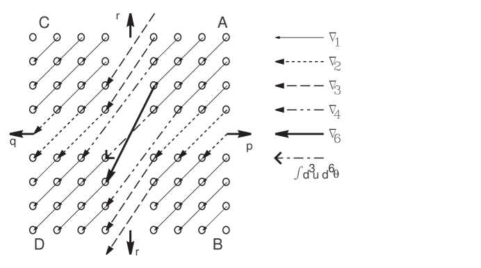
Figure 1: ${\mathfrak{vle}}(3|6)$ form modules and morphisms. First quadrant: $\Omega_{A}(p,r)=(p,r)=T(p,0;r;2p-3r)$. Second quadrant: $\Omega_{B}(p,r)=(p,-r)=T(p,0;r;2p+3r+6)$. Fourth quadrant: $\Omega_{C}(q,r)=(-q,r)=T(0,q;r;-2q-3r-6)$. Third quadrant: $\Omega_{D}(q,r)=(-q,-r)=T(0,q;r;-2q+3r)$.

3 ${\mathfrak{mb}}(3|8)$

Consider ${\mathbb{C}}^{3|8}$ with basis spanned by three even coordinates $u^{i}$, $i=1,2,3$, six odd coordinates $\theta_{ia}$, and two more odd coordinates $\vartheta^{a}$. Let $\deg\theta_{ia}=1$, $\deg u^{i}=2$ and $\deg\vartheta^{a}=3$. The graded Heisenberg algebra has the non-zero relations

$$\{\eth_{b},\vartheta^{a}\}=\delta^{a}_{b},\qquad[\partial_{j},u^{i}]=\delta^{i}_{j},\qquad\{d^{ia},\theta_{jb}\}=\delta^{i}_{j}\delta^{a}_{b},$$ (3.63)

where $\partial_{i}=\partial/\partial u^{i}$, $d^{ia}=\partial/\partial\theta_{ia}$, and $\eth_{a}=\partial/\partial\vartheta_{a}$. The vector fields

$$D^{ia} = d^{ia}-3\epsilon^{ijk}\theta^{a}_{j}\partial_{k}+\epsilon^{ijk}\theta^{a}_{j}\theta^{b}_{k}\eth_{b}-u^{i}\eth^{a},$$

$$E_{i} = \partial_{i}-\theta^{a}_{i}\eth_{a},$$ (3.64)

$$F^{a} = \eth_{a},$$

satisfy the nilpotent Lie superalgebra $\tilde{\mathfrak{g}}_{-}$:

$$\{D^{ia},D^{jb}\} = -6\epsilon^{ijk}\epsilon^{ab}E_{k},$$

$${[}D^{ia},E_{j}] = 2\delta^{i}_{j}F^{a},$$

and all other brackets vanish. Any vector field in ${\mathfrak{vect}}(3|8)$ has the form

$$X=R^{a}\eth_{a}+Q^{i}\partial_{i}+P_{ia}d^{ia}=\widetilde{R}^{a}\eth_{a}+\widetilde{Q}^{i}E_{i}+P_{ia}D^{ia},$$ (3.66)

where

$$\widetilde{Q}^{i} = Q^{i}+3(-)^{X}\epsilon^{ijk}\theta^{a}_{j}P_{ka},$$

$$\widetilde{R}^{a} = R^{a}+(-)^{X}\theta^{a}_{i}Q^{i}+2\epsilon^{ijk}\theta^{a}_{i}\theta^{b}_{j}P_{kb}-u^{i}P^{a}_{i}.$$

${\mathfrak{mb}}(3|8)$ is the subalgebra of ${\mathfrak{vect}}(3|8)$ which preserves the dual Pfaff equation $D^{ia}=0$, where $D^{ia}$ was defined in (3.64). In other words, $X\in{\mathfrak{mb}}(3|8)$ iff

$$[X,D^{ia}]=-(-)^{X}D^{ia}P_{jb}D^{jb},$$ (3.68)

which leads to the conditions

$$D^{ia}\widetilde{Q}^{j} = 6(-)^{X}\epsilon^{ijk}P^{a}_{k},$$

$$D^{ia}\widetilde{R}^{b} = -2(-)^{X}\epsilon^{ab}\widetilde{Q}^{i}.$$

In particular, we have the symmetry relations

$$D^{ia}\widetilde{Q}^{j} = -D^{ja}\widetilde{Q}^{i},$$ (3.70)

$$D^{ia}\widetilde{R}^{b} = -D^{ib}\widetilde{R}^{a}.$$

Alternatively, ${\mathfrak{mb}}(3|8)$ may be defined as the subalgebra of ${\mathfrak{vect}}(3|8)$ under which the forms

$$\alpha^{i} = du^{i}+3\epsilon^{ijk}\theta^{a}_{j}d\theta_{ka},$$

$$\beta^{a} = d\vartheta^{a}-u^{i}d\theta^{a}_{i}+\theta^{a}_{i}du^{i}+2\epsilon^{ijk}\theta^{a}_{i}\theta^{b}_{j}d\theta_{kb}.$$

transform as

$${\cal L}_{X}\alpha^{i} = E_{j}\widetilde{Q}^{i}\alpha^{j}-(-)^{X}\eth_{a}\widetilde{Q}^{i}\beta^{a},$$

$${\cal L}_{X}\beta^{a} = (-)^{X}\eth_{b}\widetilde{R}^{a}\beta^{b}.$$

Explicitly,

$$X \equiv M_{f}=f^{a}\eth_{a}+\hbox{$1\over 4$}(-)^{f}D^{ia}f_{a}E_{i}+\hbox{${1\over 48}$}\epsilon_{ijk}D^{i}_{a}D^{jb}f_{b}D^{ka},$$ (3.73)

where $f=f^{a}(\theta,u,\vartheta)\eth_{a}$ is a vector field acting on ${\mathbb{C}}^{3|8}$, $D^{ia}f^{b}=-D^{ib}f^{a}$ and $D^{ia}D^{jb}f_{b}=-D^{ja}D^{ib}f_{b}$. Note that $(-)^{f}=+1$ if $f$ is an even vector field, i.e. $f^{a}$ is an odd function.

The ${\mathfrak{mb}}(3|8)$ tensor modules are labelled by the ${\mathfrak{g}}_{0}=sl(3)\!\oplus\!sl(2)\!\oplus\!gl(1)$ weights $(p,q;r;z)$, $p,q,r\in{\mathbb{N}}$, $z\in{\mathbb{Z}}$, where $p\pi_{1}+q\pi_{2}$ is an $sl(3)$ weight, $r$ is an $sl(2)$ weight and $z$ is a $gl(1)$ weight (the eigenvalue of the grading operator). A typical element in the tensor module $T(p,q;r;z)$ has the form $f(\theta,u)\phi^{{i_{1}..i_{p}}|{a_{1}..a_{r}}}_{j_{1}..j_{q}}$, where $f(\theta,u)$ is a polynomial function and $\phi^{{i_{1}..i_{p}}|{a_{1}..a_{r}}}_{j_{1}..j_{q}}$ is totally symmetric in ${i_{1}..i_{p}}$, ${j_{1}..j_{q}}$ and ${a_{1}..a_{r}}$. From (3.68) and (LABEL:mbXab) we see that among tensor modules, the differentials $\alpha^{i}\in T(1,0;0;2)$, $\beta^{a}\in T(0,0;1;3)$ and $\gamma^{ia}\in T(1,0;1;-1)$ transform particularly simply:

$${\cal L}_{X}\alpha^{i}=E_{j}\widetilde{Q}^{i}\alpha^{j},$$

$${\cal L}_{X}\beta^{a}=(-)^{X}\eth_{b}\widetilde{R}^{a}\beta^{b},$$ (3.74)

$${\cal L}_{X}\gamma^{ia}=-(-)^{X}D^{ia}P_{jb}\gamma^{jb}.$$

The transformation law for $\alpha^{i}$ has been modified compared to (LABEL:mbXab); this is permissible because $\beta^{a}$ transforms irreducibly by itself.

Dual differentials $\bar{\alpha}_{i}\in T(0,1;0;-2)$, $\bar{\beta}_{a}\in T(0,0;1;-3)$ and $\bar{\gamma}_{ia}\in T(0,1;1;1)$ transform as

$${\cal L}_{X}\bar{\alpha}_{i}=-E_{i}\widetilde{Q}^{j}\bar{\alpha}_{j},$$

$${\cal L}_{X}\bar{\beta}_{a}=-(-)^{X}\eth_{a}\widetilde{R}^{b}\bar{\beta}_{b},$$ (3.75)

$${\cal L}_{X}\bar{\gamma}_{ia}=(-)^{X}D^{jb}P_{ia}\bar{\gamma}_{jb}.$$

If we assume that $\alpha^{i}$, $\beta^{a}$ and $\bar{\gamma}_{ia}$ are fermions, we can construct a scalar density $v=\alpha^{1}\alpha^{2}\alpha^{3}=\beta^{1}\beta^{2}=\bar{\gamma}_{11}\bar{\gamma}_{12}\bar{\gamma}_{21}\bar{\gamma}_{22}\bar{\gamma}_{31}\bar{\gamma}_{32}$; $v\in T(0,0;0;6)$ and its dual $\bar{v}\in T(0,0;0;-6)$ transform as

$${\cal L}_{X}v = E_{i}\widetilde{Q}^{i}v=(-)^{X}\eth_{a}\widetilde{R}^{a}v=(-)^{X}D^{ia}P_{ia}v,$$

$${\cal L}_{X}\bar{v} = -E_{i}\widetilde{Q}^{i}\bar{v}=-(-)^{X}\eth_{a}\widetilde{R}^{a}\bar{v}=-(-)^{X}D^{ia}P_{ia}\bar{v}.$$

Define the weight $z$ and the degree $\deg$ by

$$\begin{array}[]{l|cccccccccccccc}&\theta_{ia}&u^{i}&\vartheta^{a}&d^{ia}&\partial_{i}&\eth_{a}&\alpha^{i}&\bar{\alpha}_{j}&\beta^{a}&\bar{\beta}_{a}&\gamma^{ia}&\bar{\gamma}_{ia}&v&\bar{v}\\ \hline\cr z&0&0&0&0&0&0&2&-2&3&-3&-1&1&6&-6\\ \deg&1&2&3&-1&-2&-3&2&-2&3&-3&-1&1&6&-6\\ \end{array}$$

As for ${\mathfrak{vle}}(3|6)$, we build form modules using the elementary differentials (3.74). The action of the morphisms on the differentials and their duals is given by

$$\alpha^{i}\bar{\alpha}_{j}=\bar{\alpha}_{j}\alpha^{i}=\delta^{i}_{j}, \beta^{a}\bar{\beta}_{b}=\bar{\beta}_{b}\beta^{a}=\delta^{a}_{b},$$

$$\gamma^{ia}\bar{\gamma}_{jb}=\bar{\gamma}_{jb}\gamma^{ia}=\delta^{i}_{j}\delta^{a}_{b}, v\bar{v}=\bar{v}v=1.$$

A form may not contain differentials and dual differentials of the same type. Since there are three types of differentials, apart from the scalar density $v$, one might try to write down form depending on four parameters, e.g.

$$\omega=\omega^{{i_{1}..i_{q}}|{a_{1}..a_{r}}}(\theta,u,\vartheta)\bar{\alpha}_{i_{s+1}}...\bar{\alpha}_{i_{q}}\bar{\beta}_{a_{s+1}}...\bar{\beta}_{a_{r}}\bar{\gamma}_{i_{1}a_{1}}...\bar{\gamma}_{i_{s}a_{s}}v^{k}.$$ (3.78)

However, when one demands ${\mathfrak{g}}$ invariance it turns out that $\alpha^{i}$ and $\bar{\alpha}_{j}$ can not be used. Eq. (2.34) is replaced by

$$D^{ia}E_{k}\widetilde{Q}^{j}+D^{ja}E_{k}\widetilde{Q}^{i}=2(\delta^{i}_{k}F^{a}\widetilde{Q}^{j}+\delta^{j}_{k}F^{a}\widetilde{Q}^{i})\neq 0,$$ (3.79)

because $[D^{ia},E_{j}]=2\delta^{i}_{j}F^{a}$ from (LABEL:mb-). Hence the candidate form modules are built only from differentials $\beta^{a}$, $\gamma^{ia}$, $v$, and their duals.

After tedious calculations, completely analogous to the ${\mathfrak{vle}}(3|6)$ case, we find the following form modules:

$$\begin{array}[]{|c|c|c|c|}\hline\cr\hbox{Form}&z&\hbox{Basis}&\hbox{Condition}\\ \hline\cr\Omega_{A}(p,r)&-4p+3r-6&\gamma^{i_{1}a_{1}}...\gamma^{i_{p}a_{p}}\beta^{a_{p+1}}...\beta^{a_{r}}\bar{v}&r\geq p\\ &&\gamma^{i_{1}a_{1}}...\gamma^{i_{p}a_{p}}\bar{\beta}_{a_{r+1}}...\bar{\beta}_{a_{p}}\bar{v}&r\leq p\\ \Omega_{B}(p,r)&-4p-3r-12&\gamma^{i_{1}a_{r+1}}...\gamma^{i_{p}a_{r+p}}\bar{\beta}_{a_{1}}...\bar{\beta}_{a_{p+r}}\bar{v}^{2}&\\ \Omega_{C}(q,r)&4q+3r+6&\bar{\gamma}_{i_{1}a_{r+1}}...\bar{\gamma}_{i_{q}a_{r+q}}\beta^{a_{1}}...\beta^{a_{q+r}}v&\\ \Omega_{D}(q,r)&4q-3r&\bar{\gamma}_{i_{1}a_{1}}...\bar{\gamma}_{i_{q}a_{q}}\bar{\beta}_{a_{q+1}}...\bar{\beta}_{a_{r}}&r\geq q\\ &&\bar{\gamma}_{i_{1}a_{1}}...\bar{\gamma}_{i_{q}a_{q}}\beta^{a_{r+1}}...\beta^{a_{q}}&r\leq q\\ \hline\cr\end{array}$$ (3.87)

where $p,q,r\geq 0$ and $z$ is the eigenvalue of the grading operator.

According to the principles set out in the introduction, candidate ${\mathfrak{g}}$-invariant morphisms are differential operators which only involve the fermionic derivative $D^{ia}$, have degree zero, and are invariant under ${\mathfrak{g}}_{0}=sl(3)\!\oplus\!sl(2)\!\oplus\!gl(1)$. The complete list of such morphisms is obtained from (LABEL:vlemorph) by the substitutions

$$\alpha^{i}=\gamma^{ia}\bar{\beta}_{a}v,\qquad\bar{\alpha}_{i}=\bar{\gamma}_{ia}\beta^{a}\bar{v}.$$ (3.88)

Thus,

$$\nabla_{1} = \bar{\gamma}_{ia}D^{ia},$$

$$\nabla_{2} = \epsilon_{ab}\bar{\gamma}_{ic}\bar{\gamma}_{jd}\beta^{c}\beta^{d}\bar{v}D^{ia}D^{jb},$$

$$\nabla_{3} = \epsilon_{ijk}\bar{\beta}_{a}\bar{\beta}_{b}\bar{\beta}_{c}v^{2}D^{ia}D^{jb}D^{kc},$$

$$\nabla_{4} = \epsilon_{ijk}\epsilon_{cd}\bar{\gamma}_{la}\bar{\beta}_{b}vD^{ia}D^{jb}D^{kc}D^{ld},$$

$$\nabla_{6} = \epsilon_{ijk}\epsilon_{lmn}\epsilon_{be}\epsilon_{cf}\bar{\beta}_{a}\bar{\beta}_{d}v^{2}D^{ia}D^{jb}D^{kc}D^{ld}D^{me}D^{nf},$$

$$\hbox{$\int$}_{\theta} = \epsilon_{ijk}\epsilon_{lmn}\epsilon_{ad}\epsilon_{be}\epsilon_{cf}vD^{ia}D^{jb}D^{kc}D^{ld}D^{me}D^{nf}.$$

To fill in the missing morphisms, we again choose from the candidate list above, and make sure to match powers of $v$. This works out in the same way as for ${\mathfrak{vle}}(3|6)$, except for the $\nabla_{6}$ arrow. The relevant weights are

$$\begin{array}[]{c|ccc}&\nabla_{6}&\Omega_{A}(0,1)&\Omega_{D}(0,1)\\ \hline\cr z({\mathfrak{vle}}(3|6))&6&-3&3\\ z({\mathfrak{mb}}(3|8))&6&-3&-3\\ \end{array}$$

Thus

$$\nabla_{6}:\Omega_{A}(0,1)\to\Omega_{D}(0,1)$$

is a well-defined ${\mathfrak{vle}}(3|6)$ morphism, because $z(\nabla_{6})+z_{A}(0,1)=z_{D}(0,1)$, but it is not an ${\mathfrak{mb}}(3|8)$ morphism. However, since $z_{A}(0,1)=z_{D}(0,1)$ in ${\mathfrak{mb}}(3|8)$, the $\nabla_{6}$ arrow can be replaced by the identity map.

To summarize:

Theorem 3.1

The degenerate ${\mathfrak{mb}}(3|8)$ tensor modules are $\Omega_{A}(p,r)=\break T(p,0;r;-4p+3r-6)$, $\Omega_{B}(p,r)=T(p,0;r;-4p-3r-12)$, $\Omega_{C}(q,r)=T(0,q;r;4q+3r+6)$, $\Omega_{D}(q,r)=T(0,q;r;4q-3r)$, ($p,q,r\geq 0$). The morphisms are the same as in (2.61), except that the $\nabla_{6}$ arrow is replaced by the identity map (since $\Omega_{A}(0,1)=\Omega_{D}(0,1)=T(0,0;1;-3)$). The integral morphism reads

$$\int d^{3}ud^{6}\theta d^{2}\vartheta\,:\Omega_{A}(0,0) \to \Omega_{D}(0,0),$$

$$\omega(\theta,u,\vartheta)\bar{v} \mapsto \int d^{3}ud^{6}\theta d^{2}\vartheta\,\omega(\theta,u,\vartheta).$$

The morphisms can be illustrated by the Figure 1, which is the same as for ${\mathfrak{vle}}(3|6)$. This result is superficially different from what Kac and Rudakov find [15], because they work in a contragredient formalism. Agreement is found if we redefine $(p,q)\to(q,p)$, $z\to-z$, $\Omega_{A}\leftrightarrow\Omega_{D}$, and $\Omega_{B}\leftrightarrow\Omega_{C}$. Again, they do not consider the non-local integral, which explains the hole in the middle of their Figure 1.

4 ${\mathfrak{ksle}}(5|10)$

Consider ${\mathbb{C}}^{5|10}$ with basis spanned by five even coordinates $u^{i}$, $i=1,2,3,4,5$ and ten odd coordinates $\theta_{ij}=-\theta_{ji}$. Let $\deg\theta_{ij}=1$ and $\deg u^{i}=2$. The graded Heisenberg algebra has the non-zero relations

$$[\partial_{j},u^{i}]=\delta^{i}_{j},\qquad\{d^{ij},\theta_{kl}\}=\delta^{i}_{k}\delta^{j}_{l}-\delta^{j}_{k}\delta^{i}_{l},$$ (4.90)

where $\partial_{i}=\partial/\partial u^{i}$ and $d^{ij}=-d^{ji}=\partial/\partial\theta_{ij}$. Consider the vector fields

$$D^{ij} = d^{ij}+\hbox{$1\over 2$}\epsilon^{ijklm}\theta_{kl}\partial_{m},$$

$$E_{k} = \partial_{k},$$

which generate the superalgebra

$$\{D^{ij},D^{kl}\} = 2\epsilon^{ijklm}E_{m},$$

$${[}D^{ij},E_{k}] = [E_{k},E_{l}]=0.$$

Any vector field in ${\mathfrak{vect}}(5|10)$ has the form

$$X=Q^{i}\partial_{i}+\hbox{$1\over 2$}P_{ij}d^{ij}=\widetilde{Q}^{i}\partial_{i}+\hbox{$1\over 2$}P_{ij}D^{ij},$$ (4.93)

where the $1\over 2$ is necessary to avoid double counting and

$$\widetilde{Q}^{i} = Q^{i}+\hbox{$1\over 4$}(-)^{X}\epsilon^{ijklm}\theta_{jk}P_{lm}.$$ (4.94)

${\mathfrak{ksle}}(5|10)$ is the subalgebra of ${\mathfrak{svect}}(5|10)$ (divergence-free vector fields) which preserve the dual Pfaff equation $D^{ij}=0$. For convenience, we will adjoin the grading operator $Z=2u^{i}\partial_{i}+\hbox{$1\over 2$}\theta_{ij}d^{ij}$ to ${\mathfrak{ksle}}(5|10)$, and thus consider the non-simple algebra $\overline{{\mathfrak{ksle}}(5|10)}=({\bf{{5}}},{\bf{{10^{*}}}},gl(5))_{*}$. Hence $X\in\overline{{\mathfrak{ksle}}(5|10)}$ iff

$$[X,D^{ij}]=-\hbox{$1\over 2$}(-)^{X}D^{ij}P_{kl}D^{kl}$$ (4.95)

which leads to the condition

$$D^{ij}\widetilde{Q}^{k}=(-)^{X}\epsilon^{ijklm}P_{lm}.$$ (4.96)

In particular, we have the symmetry relations

$$D^{ij}\widetilde{Q}^{k}=D^{jk}\widetilde{Q}^{i}=-D^{ik}\widetilde{Q}^{j}.$$ (4.97)

Alternatively, ${\mathfrak{ksle}}(5|10)$ can be defined as the vector fields which preserve the form

$$\alpha^{i}=du^{i}+\hbox{$1\over 4$}\epsilon^{ijklm}\theta_{jk}d\theta_{lm}$$ (4.98)

up to a factor:

$${\cal L}_{X}\alpha^{i}=\partial_{j}\widetilde{Q}^{i}\alpha^{j}.$$ (4.99)

Explicitly,

$$X\equiv U_{f}=f^{i}\partial_{i}+\hbox{$1\over 24$}(-)^{f}\epsilon_{ijklm}D^{ij}f^{k}D^{lm},$$ (4.100)

where $f=f^{i}(\theta,u)\partial_{i}$ is a vector field acting on ${\mathbb{C}}^{5|10}$, $D^{ij}f^{k}=D^{jk}f^{i}=-D^{ik}f^{j}$, and $\partial_{i}f^{i}=0$.

The $\overline{{\mathfrak{ksle}}(5|10)}$ tensor modules are labelled by the $sl(5)$ weights $(p,q,r,s)=p\pi_{1}+q\pi_{2}+r\pi_{3}+s\pi_{4}$, $p,q,r,s\in{\mathbb{N}}$, and a $gl(1)$ weight $z\in{\mathbb{Z}}$ (the eigenvalue of the grading operator). A typical element in the tensor module $T(p,q,r,s;z)$ has the form $f(\theta,u)\phi^{{i_{1}..i_{p}}|{k_{1}l_{1}..k_{q}l_{q}}}_{{j_{1}..j_{s}}|{m_{1}n_{1}..m_{r}n_{r}}}$, where $f(\theta,u)$ is a polynomial function and $\phi^{{i_{1}..i_{p}}|{k_{1}l_{1}..k_{q}l_{q}}}_{{j_{1}..j_{s}}|{m_{1}n_{1}..m_{r}n_{r}}}$ is totally symmetric in ${i_{1}..i_{p}}$, ${k_{1}l_{1}..k_{q}l_{q}}$, ${m_{1}n_{1}..m_{r}n_{r}}$, and ${j_{1}..j_{s}}$, and anti-symmetric under $k_{1}l_{1}\to l_{1}k_{1}$ and $m_{1}n_{1}\to n_{1}m_{1}$, etc. From (4.95) and (4.99) we see that among tensor modules, the differentials $\alpha^{i}\in T(1,0,0,0;2)$ and $\gamma^{ij}\in T(0,1,0,0;-1)$ transform particularly simply:

$${\cal L}_{X}\alpha^{i}=\partial_{j}\widetilde{Q}^{i}\alpha^{j},\qquad{\cal L}_{X}\gamma^{ij}=-\hbox{$1\over 2$}(-)^{X}D^{ij}P_{kl}\gamma^{kl}.$$ (4.101)

Dual differentials $\bar{\alpha}_{i}\in T(0,0,0,1;-2)$ and $\bar{\gamma}_{ij}\in T(0,0,1,0;1)$ transform as

$${\cal L}_{X}\bar{\alpha}_{i}=-\partial_{i}\widetilde{Q}^{j}\bar{\alpha}_{j},\qquad{\cal L}_{X}\bar{\gamma}_{ij}=\hbox{$1\over 2$}(-)^{X}D^{kl}P_{ij}\bar{\gamma}_{kl}.$$ (4.102)

If we assume that $\alpha^{i}$ and $\bar{\gamma}_{ia}$ are fermions, we can construct a density form $v=\alpha^{1}\alpha^{2}\alpha^{3}\alpha^{4}\alpha^{5}=\bar{\gamma}_{12}\bar{\gamma}_{13}\bar{\gamma}_{14}\bar{\gamma}_{15}\bar{\gamma}_{23}\bar{\gamma}_{24}\bar{\gamma}_{25}\bar{\gamma}_{34}\bar{\gamma}_{35}\bar{\gamma}_{45}$; $v\in T(0,0,0,0;10)$ and its dual $\bar{v}\in T(0,0,0,0;-10)$ transform as

$${\cal L}_{X}v = \partial_{i}\widetilde{Q}^{i}v=\hbox{$1\over 2$}(-)^{X}D^{ij}P_{ij}v,$$

$${\cal L}_{X}\bar{v} = -\partial_{i}\widetilde{Q}^{i}\bar{v}=-\hbox{$1\over 2$}(-)^{X}D^{ij}P_{ij}\bar{v}.$$

Forms can be constructed from the differentials (4.101), with the following action on the differentials and their duals:

$$\alpha^{i}\bar{\alpha}_{j}=\bar{\alpha}_{j}\alpha^{i}=\delta^{i}_{j},\quad\gamma^{ij}\bar{\gamma}_{kl}=\bar{\gamma}_{kl}\gamma^{ij}=\delta^{i}_{k}\delta^{j}_{l}-\delta^{i}_{l}\delta^{j}_{k},\quad v\bar{v}=\bar{v}v=1.$$ (4.104)

Therefore, a form may not contain differentials and dual differentials of the same type. The basic form is

$$\omega = \omega^{{i_{1}..i_{s}}|{j_{1}k_{1}..j_{r}k_{r}}}(\theta,u)\bar{\alpha}_{i_{1}}...\bar{\alpha}_{i_{s}}\bar{\gamma}_{j_{1}k_{1}}...\bar{\gamma}_{j_{r}k_{r}},$$

where $\omega_{{i_{1}..i_{s}}|{j_{1}k_{1}..j_{r}k_{r}}}(\theta,u)$ is a polynomial function, totally symmetric in ${i_{1}..i_{s}}$, anti-symmetric under $j_{m}k_{m}\leftrightarrow k_{m}j_{m}$, and symmetric under $j_{m}k_{m}j_{n}k_{n}\leftrightarrow j_{n}k_{n}j_{m}k_{m}$. Clearly, $\omega\in T(0,0,r,s;r-2s)\equiv\Omega_{D}(s,r)$. There is a morphism $\nabla_{1}:\Omega_{D}(s,r)\to\Omega_{D}(s,r+1)$, defined by

$$\nabla_{1}\omega=\mathbf{S}(D^{lm}\omega^{{i_{1}..i_{s}}|{j_{1}k_{1}..j_{r}k_{r}}}(\theta,u))\bar{\alpha}_{i_{1}}...\bar{\alpha}_{i_{s}}\bar{\gamma}_{j_{1}k_{1}}...\bar{\gamma}_{j_{r}k_{r}}\bar{\gamma}_{lm},$$ (4.105)

where the indices $lm$ are symmetrized with ${j_{1}k_{1}..j_{r}k_{r}}$, e.g.

$$\mathbf{S}(D^{lm}\omega^{{i_{1}..i_{s}}|}) = D^{lm}\omega^{{i_{1}..i_{s}}|},$$

$$\mathbf{S}(D^{lm}\omega^{{i_{1}..i_{s}}|j_{1}k_{1}}) = D^{lm}\omega^{{i_{1}..i_{s}}|j_{1}k_{1}}+D^{j_{1}k_{1}}\omega^{{i_{1}..i_{s}}|lm},$$

$$\mathbf{S}(D^{lm}\omega^{{i_{1}..i_{s}}|j_{1}k_{1}j_{2}k_{2}}) = D^{lm}\omega^{{i_{1}..i_{s}}|j_{1}k_{1}j_{2}k_{2}}+$$

$$+D^{j_{1}k_{1}}\omega^{{i_{1}..i_{s}}|lmj_{2}k_{2}}+D^{j_{2}k_{2}}\omega^{{i_{1}..i_{s}}|lmj_{1}k_{1}}.$$

The verification that (4.105) indeed defines a morphism involves (4.95) in the form

$$(D^{ij}X)=\hbox{$1\over 2$}D^{ij}P_{kl}D^{kl},$$ (4.107)

(4.97) and $[D^{ij},E_{k}]=0$.

Using similar calculations one proves that there are four sectors of form modules, as summarized in the following table. Here $p,q,r,s\geq 0$ and the weight $z$ is the eigenvalue of the grading operator.

$$\begin{array}[]{|c|c|c|c|}\hline\cr\hbox{Form}&\hbox{$sl(5)$ weight}&z&\hbox{Basis}\\ \hline\cr\Omega_{A}(p,q)&(p,q,0,0)&2p-q&\alpha^{i_{1}}...\alpha^{i_{p}}\gamma^{j_{1}k_{1}}...\gamma^{j_{q}k_{q}}\\ \Omega_{B}(p,r)&(p,0,r,0)&2p+r&\alpha^{i_{1}}...\alpha^{i_{p}}\bar{\gamma}_{j_{1}k_{1}}...\bar{\gamma}_{j_{r}k_{r}}\\ \Omega_{C}(s,q)&(0,q,0,s)&-2s-q&\bar{\alpha}_{i_{s}}...\bar{\alpha}_{i_{s}}\gamma^{j_{1}k_{1}}...\gamma^{j_{q}k_{q}}\\ \Omega_{D}(s,r)&(0,0,r,s)&-2s+r&\bar{\alpha}_{i_{1}}...\bar{\alpha}_{i_{s}}\bar{\gamma}_{j_{1}k_{1}}...\bar{\gamma}_{j_{r}k_{r}}\\ \hline\cr\end{array}$$

The first-order morphisms which have been constructed are of the form

$$\begin{array}[]{lll}\nabla_{1}:&\Omega_{A}(p,q)\to\Omega_{A}(p,q-1),&q\neq 0\\ &\Omega_{B}(p,r)\to\Omega_{B}(p,r+1),&\\ &\Omega_{C}(s,q)\to\Omega_{C}(s,q-1),&q\neq 0\\ &\Omega_{D}(s,r)\to\Omega_{D}(s,r+1),&\\ \end{array}$$ (4.112)

Note that

$$\Omega_{A}(p,0)=\Omega_{B}(p,0), \Omega_{A}(0,q)=\Omega_{C}(0,q),$$

$$\Omega_{D}(s,0)=\Omega_{C}(s,0), \Omega_{D}(0,r)=\Omega_{B}(0,r),$$

because no explicit factors of the scalar differential $v$ appear. Therefore, all morphisms are already connected into infinite complexes. Nevertheless, there are more morphisms. First of all, the integral is ${\mathfrak{vect}}(5|10)$ invariant, so there is a map

$$\int d^{5}ud^{10}\theta\,:\Omega_{X}(0,0) \to \Omega_{X}(0,0),$$

$$\omega(\theta,u) \mapsto \int d^{5}ud^{10}\theta\,\omega(\theta,u)$$

(the module at the origin is the same for all four sectors). Moreover, there exist further differential operators that only involve the fermionic derivative $D^{ij}$, have degree zero, and are invariant under ${\mathfrak{g}}_{0}=sl(5)\!\oplus\!gl(1)$. The complete list of such morphisms is given by

$$\nabla_{1} = \bar{\gamma}_{ij}D^{ij},$$

$$\nabla_{2} = \epsilon_{ijklm}\epsilon_{npqrs}\alpha^{i}\alpha^{n}D^{jp}D^{kq}D^{lr}D^{ms},$$ (4.115)

$$\hbox{$\int$}_{\theta} = vD^{12}D^{13}D^{14}D^{15}D^{23}D^{24}D^{25}D^{34}D^{35}D^{45}.$$

It is natural to conjecture that $\nabla_{2}$ acts on the modules with $q=0$ and $r=0$, which thus have two ingoing and two outgoing morphisms:

$$\begin{array}[]{rl}\nabla_{2}:&\Omega_{A}(p,0)\to\Omega_{B}(p+2,0),\\ \nabla_{2}:&\Omega_{C}(s,0)\to\Omega_{D}(s-2,0),\\ \end{array}$$

The situation (conjectured for $\nabla_{2}$ but proven for $\nabla_{1}$) is summarized in Figure 2.

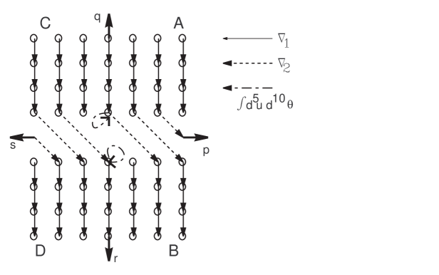
Figure 2: ${\mathfrak{ksle}}(5|10)$ form modules and morphisms. The modules on the $q=0$ or $r=0$ axis has been split into two to give a clearer view of the arrows. The loop at the origin is the integral morphism. Existence of the arrows denoted by $\nabla_{2}$ is conjectural. First quadrant: $\Omega_{A}(p,q)=(p,q)=T(p,q,0,0;2p-q)$. Second quadrant: $\Omega_{B}(p,r)=(p,-r)=T(p,0,r,0;2p+r)$. Fourth quadrant: $\Omega_{C}(s,q)=(-s,q)=T(0,q,0,s;-2s-q)$. Third quadrant: $\Omega_{D}(s,r)=(-s,-r)=T(0,0,r,s;-2s+r)$.

This result disagrees with what Kac and Rudakov find in [15]. They find three sectors, with $sl(5)$ weights

$$A=(p,q,0,0),B=(0,0,r,s),C=(p,0,0,s).$$ (4.116)

The first two sectors are the same as my $\Omega_{A}$ and $\Omega_{D}$ forms, and the omission of $\Omega_{B}$ and $\Omega_{C}$ is not a problem, since they only conjecture completeness of their list. However, I am not able to verify that the tensor modules of type $(p,0,0,s)$ are reducible. The alleged morphism is, in the notation of the present paper,

$$\nabla_{C}=(\bar{\alpha}_{i}{\partial\over\partial\alpha^{j}}-\bar{\alpha}_{j}{\partial\over\partial\alpha^{i}})D^{ij},$$ (4.117)

when acting on tensor fields of the form

$$\omega^{j_{1}..j_{s}}_{i_{1}..i_{p}}\alpha^{i_{1}}...\alpha^{i_{p}}\bar{\alpha}_{j_{1}}...\bar{\alpha}_{j_{s}}.$$ (4.118)

When acting on pure powers, i.e. modules which involve either $\alpha^{i}$ or $\bar{\alpha}_{j}$ but not both, we have identified $\alpha^{i}=\partial/\partial\bar{\alpha}_{j}$ and $\bar{\alpha}_{j}=\partial/\partial\alpha^{i}$. This identification is not possible here, because it would make $\nabla_{C}\equiv 0$. Moreover, I have verified that the simplest case,

$$\nabla_{C}:(1,0,0,0) \to (0,0,0,1),$$

$$\omega_{i}\alpha^{i} \mapsto D^{ij}\omega_{i}\bar{\alpha}_{j}$$

is in fact not ${\mathfrak{ksle}}(5|10)$ invariant. Hence I conclude that tensor modules of type C are not form modules.

5 A second-gauged standard model

The potential interest of the exceptional superalgebras is based on the following two observations:

1. The grade zero subalgebra of ${\mathfrak{vle}}(3|6)$ and ${\mathfrak{mb}}(3|8)$ is ${\mathfrak{g}}_{0}=sl(3)\!\oplus\!sl(2)\!\oplus\!gl(1)$, i.e. the non-compact form of the symmetries of the standard model in particle physics.

2. ${\mathfrak{mb}}(3|8)$ is the unique superalgebra of maximal depth $3$ in its consistent gradation.

Even if depth in the technical sense does not necessarily mean profound, the technical and informal usages of the word are related; maximal depth essentially means that the algebra has the most intricate and beautiful structure possible. The richest conceivable local symmetry is hence intimately related to the symmetries of the standard model; there is a 1-1 correspondence between irreducible modules. It is therefore very tempting to construct a gauge theory with a local ${\mathfrak{mb}}(3|8)$ symmetry, and in this section a first step in this direction is taken. We do not limit ourselves to the exceptional superalgebras, but consider the general case of replacing a finite-dimensional symmetry ${\mathfrak{g}}_{0}$ by a quite general class of infinite-dimensional symmetries ${\mathfrak{g}}$. Due to the shortage of letters, indices in this section are not related to indices with identical names in previous sections. Moreover, we ignore all superalgebra sign factors and pretend that we are dealing with ordinary Lie algebras. This is of course not correct, but keeping track of signs will only complicate matters and obscure the main points.

Let $J^{a}$, $a=1,2,...,\dim{\mathfrak{g}}_{0}$ be the generators of the finite-dimensional Lie algebra ${\mathfrak{g}}_{0}\subset gl({n|m})$ with structure constants $f^{ab}{}_{c}$:

$$[J^{a},J^{b}]=f^{ab}{}_{c}J^{c}.$$ (5.120)

Let $y^{i}$, $i=1,...,n,n+1,...n+m$ be the coordinates of ${\mathbb{C}}^{n|m}$, and let $\partial_{i}=\partial/\partial y^{i}$ be the corresponding derivatives. Then ${\mathfrak{g}}_{0}$ can be realized as vector fields of the form $J^{a}=-\varrho^{ja}_{i}y^{i}\partial_{j}$. Let $D_{i}=\partial/\partial y^{i}+...$ be $n+m$ first order derivatives, which generate a closed nilpotent algebra $\tilde{\mathfrak{g}}_{-}$ which is also a ${\mathfrak{g}}_{0}$ module:

$$[D_{i},D_{j}] = g_{ij}{}^{k}D_{k}$$

$${[}J^{a},D_{j}] = \varrho^{ia}_{j}D_{i}.$$

The structure constants $g_{ij}{}^{k}$ and $\varrho^{ia}_{j}$ are assumed to respect the grading, i.e. $g_{ij}{}^{k}=0$ unless $\deg y^{i}+\deg y^{j}=\deg y^{k}$ and $\varrho^{ia}_{j}=0$ unless $\deg y^{i}=\deg y^{j}$.

Any vector field $X\in{\mathfrak{vect}}({n|m})$ can be expanded in the $D_{i}$ basis: $X=X^{i}(y)D_{i}$. Clearly,

$$[X,Y]=X^{i}D_{i}Y^{j}D_{j}-Y^{j}D_{j}X^{i}D_{i}+g_{ij}{}^{k}X^{i}Y^{j}D_{k}.$$ (5.122)

Now consider the vector fields $X$ whose bracket with $D_{i}$ is of the form

$$[D_{i},X]\equiv D_{i}X^{k}D_{k}+g_{ij}{}^{k}X^{j}D_{k}=\bar{h}^{jl}_{ik}D_{j}X^{k}D_{l}$$ (5.123)

for some structure constants $\bar{h}^{jl}_{ik}$ which also preserve the grading: $\bar{h}^{jl}_{ik}=0$ unless $\deg y^{j}+\deg y^{l}=\deg y^{i}+\deg y^{k}$. Setting $\bar{h}^{jl}_{ik}=\delta^{j}_{i}\delta^{l}_{k}+h^{jl}_{ik}$, (5.123) can be rewritten as

$$g_{ij}{}^{l}X^{j}=h^{jl}_{ik}D_{j}X^{k}.$$ (5.124)

This equation defines the subalgebra ${\mathfrak{g}}\subset{\mathfrak{vect}}({n|m})$.

Define $\sigma^{i}_{ja}$ to be the inverse of the projection $\varrho^{ia}_{j}$:

$$\varrho^{ia}_{j}\sigma^{j}_{ib}=\delta^{a}_{b},\qquad\varrho^{ia}_{j}\sigma^{k}_{la}\approx\delta^{i}_{l}\delta^{k}_{j}.$$ (5.125)

The notation $\approx$ is defined to mean equality when contracted with $D_{j}X^{i}$. Thus, the second relation above should be interpreted to mean $D_{j}X^{i}=\varrho^{ia}_{j}\sigma^{k}_{la}D_{k}X^{l}$ for every $X\in{\mathfrak{g}}$. Note that this relation can not hold for arbitrary vector fields, but only for vector fields in ${\mathfrak{g}}$. It is now straightforward to prove that

$${\cal L}_{X}=X+D_{j}X^{i}\sigma^{j}_{ia}T^{a}\equiv X+D_{j}X^{i}T^{j}_{i}$$ (5.126)

satisfies $[{\cal L}_{X},{\cal L}_{Y}]={\cal L}_{[X,Y]}$, with $[X,Y]$ as in (5.122), provided that

$$\sigma^{k}_{ia}\sigma^{l}_{jb}f^{ab}{}_{c} \approx \delta^{l}_{i}\sigma^{k}_{jc}-\delta^{k}_{j}\sigma^{l}_{ic}$$

$$+h^{kl}_{mi}\sigma^{m}_{jc}-h^{lk}_{mj}\sigma^{m}_{ic}+h^{lm}_{ij}\sigma^{k}_{mc}-h^{km}_{ji}\sigma^{l}_{mc}$$

($\approx$ indicates that the relation holds when contracted with $D_{k}X^{i}D_{l}Y^{j}$, for all $X,Y\in{\mathfrak{g}}$.) There are cases were relations of this type exist; the exceptional Lie superalgebras provide examples, which follows from the explicit descriptions of their tensor modules. The generators $T^{i}_{j}$ satisfy $gl({n|m})$ weakly:

$$[T^{i}_{j},T^{k}_{l}]\approx\delta^{k}_{j}T^{i}_{l}-\delta^{i}_{l}T^{k}_{j}.$$ (5.128)

We thus have the projection ${\mathfrak{g}}\twoheadrightarrow gl({n|m}):T^{a}=\varrho^{ia}_{j}T^{j}_{i}$ and the injection ${\mathfrak{g}}\hookrightarrow gl({n|m}):T^{i}_{j}\approx\sigma^{j}_{ia}T^{a}$. The transformation laws can be read off from (5.126); e.g., a vector and a covector transform as

$${\cal L}_{X}\gamma^{i} = -X\gamma^{i}+D_{j}X^{i}\gamma^{j},$$

$${\cal L}_{X}\psi_{j} = -X\psi_{j}-D_{j}X^{i}\psi_{i}.$$

The symmetry of the gauge theory is not ${\mathfrak{g}}$ itself, but rather the associated current algebra ${\mathfrak{map}}(N,{\mathfrak{g}})$; it does not matter if ${\mathfrak{g}}=sl(3)\!\oplus\!sl(2)\!\oplus\!gl(1)$, ${\mathfrak{vle}}(3|6)$, or ${\mathfrak{mb}}(3|8)$ here. We must hence develop the representation theory of the algebra of maps from $N$-dimensional spacetime to an infinite-dimensional vectorial algebra ${\mathfrak{g}}$. There is one important complication compared to the situation when ${\mathfrak{g}}$ is finite-dimensional.

Actually, we consider the larger algebra ${{\mathfrak{vect}}(N)\ltimes{\mathfrak{map}}(N,{\mathfrak{g}})}$ obtained by adding spacetime diffeomorphisms ${\mathfrak{vect}}(N)$. This algebra is clearly a subalgebra of ${{\mathfrak{vect}}(N)\ltimes{\mathfrak{map}}(N,{\mathfrak{vect}}({n|m}))}\subset{\mathfrak{vect}}(N+{n|m})$, the algebra of diffeomorphisms in $N+{n|m}$-dimensional space which preserve the splitting into an $N$-dimensional base space and an ${n|m}$-dimensional fiber. Any such vector field can be decomposed into horizonal and vertical parts: $(\xi,X)=(\xi^{\mu}(x)\partial_{\mu},X^{i}(x,y)D_{i})$, where $x=x^{\mu}$, $\mu=1,2,...,N$, is the spacetime coordinate and $\partial_{\mu}=\partial/\partial x^{\mu}$ the corresponding derivative. The bracket in ${{\mathfrak{vect}}(N)\ltimes{\mathfrak{map}}(N,{\mathfrak{g}})}$ takes the form

$$[\xi,\eta] = \xi^{\mu}\partial_{\mu}\eta^{\nu}\partial_{\nu}-\eta^{\nu}\partial_{\nu}\xi^{\mu}\partial_{\mu},$$

$${[}\xi,X] = \xi^{\mu}\partial_{\mu}X^{i}D_{i},$$ (5.130)

$${[}X,Y] = X^{i}D_{i}Y^{j}D_{j}-Y^{j}D_{j}X^{i}D_{i}+g_{ij}{}^{k}X^{i}Y^{j}D_{k}.$$

The corresponding Lie derivatives are

$${\cal L}_{\xi} = \xi+\partial_{\nu}\xi^{\mu}T^{\nu}_{\mu},$$

$${\cal L}_{X} = X+D_{j}X^{i}\sigma^{j}_{ia}T^{a}+\epsilon\partial_{\nu}X^{i}T^{\nu}_{i},$$

where

$$[T^{\mu}_{\nu},T^{\rho}_{\sigma}] = \delta^{\rho}_{\nu}T^{\mu}_{\sigma}-\delta^{\mu}_{\sigma}T^{\rho}_{\nu},$$

$${[}T^{\mu}_{\nu},T^{\rho}_{j}] = \delta^{\rho}_{\nu}T^{\mu}_{j},$$

$${[}T^{a},T^{\mu}_{j}] = \varrho^{ia}_{j}T^{\mu}_{i},$$

$${[}T^{\mu}_{i},T^{\nu}_{j}] = [T^{\mu}_{\nu},T^{a}]=0.$$

Note the appearence of the last term in the expression for ${\cal L}_{X}$. The constant $\epsilon$ can take on any value without violating the representation condition. The point is that if we set $\epsilon\neq 0$, vectors in internal space acquire spacetime components as well. In particular, (LABEL:gp1) is replaced by

$${\cal L}_{X}\gamma^{\mu} = -X\gamma^{\mu},$$

$${\cal L}_{X}\gamma^{i} = -X\gamma^{i}+D_{j}X^{i}\gamma^{j}+\epsilon\partial_{\nu}X^{i}\gamma^{\nu},$$

$${\cal L}_{X}\psi_{\nu} = -X\psi_{\nu}-\epsilon\partial_{\nu}X^{i}\psi_{i},$$

$${\cal L}_{X}\psi_{j} = -X\psi_{j}-D_{j}X^{i}\psi_{i}.$$

Thus $(\gamma^{\mu},\gamma^{i})$ and $(\psi_{\nu},\psi_{j})$ carry reducible but indecomposable representations of ${\mathfrak{map}}(N,{\mathfrak{g}})$, with $\gamma^{\mu}$ and $\psi_{j}$ being the irreducible submodules. If we set $\epsilon=0$, assume that $X$ is of the form $X=X_{a}(x)\varrho^{ja}_{i}y^{i}\partial_{j}$, and consider the action on $y$-independent functions only, the expression for ${\cal L}_{X}$ becomes ${\cal L}_{X}=X_{a}(x)T^{a}$, which is recognized as the natural realization of the current algebra ${\mathfrak{map}}(N,{\mathfrak{g}}_{0})$. However, when we consider the full algebra ${\mathfrak{g}}$ the restriction to $y$-independent functions is not meaningful.

The standard model enjoys extreme experimental success, so any attempt to modify it must in some sense stay very close to it. A natural strategy is to start from the standard model action and make the minimal modifications necessary to elevate the ${\mathfrak{g}}_{0}$ symmetry to a ${\mathfrak{g}}$ symmetry. Focus on the Yang-Mills-Dirac part:

$$S_{D} = \int d^{N}\!x\,\bar{\psi}(x)\gamma^{\mu}{\cal D}_{\mu}\psi(x),$$

$${\cal D}_{\mu} \equiv \partial_{\mu}+A_{a\mu}(x)T^{a},$$

which leads to the massless Dirac equation $\gamma^{\mu}{\cal D}_{\mu}\psi(x)=0$. It is now tempting to simply replace the spacetime fields with functions of both $x$ and $y$: $\psi(x,y)$, $\bar{\psi}(x,y)$ and $A_{a\mu}(x,y)$. However, this does not work. One readily verifies that

$${\cal L}_{X}\partial_{\nu}\psi = -X\partial_{\nu}\psi-D_{j}X^{i}\sigma^{j}_{ia}T^{a}\partial_{\nu}\psi$$

$$-\partial_{\nu}X^{i}D_{i}\psi-\partial_{\nu}D_{j}X^{i}\sigma^{j}_{ia}T^{a}\psi.$$

The last term can be compensated by demanding that the connection $A_{a\mu}$ transforms as

$${\cal L}_{X}A_{a\mu}=-XA_{a\mu}-f^{bc}{}_{a}X_{b}A_{c\mu}-\partial_{\mu}X^{i}A_{ai}+\sigma^{j}_{ia}\partial_{\mu}D_{j}X^{i},$$ (5.136)

but the third term forces us to introduce components $D_{j}\psi$ in the internal directions as well. In other words, $(\partial_{\nu}\psi,D_{j}\psi)$ transforms as the vector $(\psi_{\nu},\psi_{j})$ in (LABEL:gp2) with $\epsilon=1$. There is no way that we can choose $\epsilon=0$ to make the vector’s spacetime components decouple from its internal components.

It is now easy to see that the simplest ${\mathfrak{g}}$-invariant generalization of (LABEL:S_D) is

$$S_{D} = \int d^{N}\!x\,d^{n|m}\!y\,\bar{\psi}(x,y)(\gamma^{\mu}{\cal D}_{\mu}+\gamma^{i}(x,y){\cal D}_{i})\psi(x,y),$$

$${\cal D}_{\mu} = \partial_{\mu}+A_{a\mu}(x,y)T^{a},$$ (5.137)

$${\cal D}_{i} = D_{i}+A_{ai}(x,y)T^{a},$$

where ${\cal L}_{X}$ acts on $\gamma^{\mu}$ as (LABEL:gp2) with $\epsilon=1$ and on $A_{a\mu}$ as (5.136), and $\psi$ and $\bar{\psi}$ transform contragrediently:

$${\cal L}_{X}\psi = -X\psi-D_{j}X^{i}\sigma^{j}_{ia}T^{a}\psi,$$

$${\cal L}_{X}\bar{\psi} = -X\bar{\psi}+D_{j}X^{i}\sigma^{j}_{ia}\bar{\psi}T^{a}.$$

Clearly, all formulas simplify if we combine spacetime and internal components into a single $(N+{n|m})$-dimensional vector. Let capital letters from the middle of the alphabeth denote combined indices, e.g. $I=(\mu,i)=1,...,N+n+m$. The Dirac action (5.137) becomes

$$S_{D} = \int d^{N}\!x\,d^{n|m}\!y\,\bar{\psi}(x,y)\hbox{${\cal D}\kern-6.82864pt/$}\psi(x,y),$$ (5.139)

where

$$\hbox{${\cal D}\kern-6.82864pt/$}\equiv\gamma^{I}(x,y){\cal D}_{I},\qquad{\cal D}_{I}=(\partial_{\mu},D_{i})+A_{aI}(x,y)T^{a}.$$ (5.140)

Given this covariant derivative we can construct the Yang-Mills field strength $F_{aIJ}T^{a}=[{\cal D}_{I},{\cal D}_{J}]$ and the Yang-Mills action

$$S_{YM}=\int d^{N}\!x\,d^{n|m}\!y\,\sqrt{g}g^{IK}g^{JL}F_{aIJ}F^{a}_{KL}.$$ (5.141)

Explicit factors of the metric $g^{IK}$ and the density $\sqrt{g}$ have been introduced. The metric is defined in terms of the gamma matrices $\gamma^{I}(x,y)=(\gamma^{\mu},\gamma^{i}(x,y))$ as usual: $\{\gamma^{I}(x,y),\gamma^{J}(x,y)\}=2g^{IJ}(x,y)$. Note that even if we may consider the spacetime components $\gamma^{\mu}$ and $g^{\mu\nu}$ to be constants (as long as we restrict spacetime diffeomorphisms ${\mathfrak{vect}}(N)$ to its Poincaré subalgebra), the internal components $\gamma^{i}(x,y)$ can not be constants because of (LABEL:gp2). We are therefore forced to consider a curved metric in internal space, even though spacetime curvature is zero. This issue will not be pursued further here.

A generic conclusion is that we can not consider spacetime to be entirely separated from the internal space; a non-zero value of the parameter $\epsilon$ in (LABEL:gp2) forces us to combine spacetime and internal indices into a single entity. However, unlike the situation in presently popular theories, spacetime and internal directions are intrinsically different from the outset.

The action $S=S_{D}+S_{YM}$ (and perhaps more terms as well) is a ${\mathfrak{g}}$-invariant generalization of the ${\mathfrak{g}}_{0}$-invariant standard model action. However, if this would be the final goal, passage from ${\mathfrak{g}}_{0}$ to the prolong ${\mathfrak{g}}=({\mathfrak{g}}_{-},{\mathfrak{g}}_{0})_{*}$ would hardly be very interesting, because all information about ${\mathfrak{g}}$ tensor modules is already encoded in ${\mathfrak{g}}_{0}$. The genuinely new information in ${\mathfrak{g}}$ is about form modules, i.e. tensor modules which are reducible even though the corresponding ${\mathfrak{g}}_{0}$ module is irreducible. So we demand that the fermions satisfy not only the massless Dirac equation

$$\hbox{${\cal D}\kern-6.82864pt/$}\psi(x,y)=0,$$ (5.142)

but also the closedness condition

$$\nabla\psi(x,y)=0,$$ (5.143)

where $\nabla$ is a ${\mathfrak{g}}$-invariant morphism of the type constructed in previous sections. It follows from $(\ref{gp2})$ that every such $\nabla$, which only involves the internal derivative $D_{i}$, can be trivially extended to a ${\mathfrak{map}}(N,{\mathfrak{g}})$-invariant morphism. It is clear that (5.143) is compatible with (5.142) and that non-zero solutions exist. Namely, a sufficient condition for (5.143) to hold is $D_{i}\psi(x,y)=0$, which makes $\psi(x,y)$ independent of the internal coordinate $y$. The Dirac equation then reduces to

$$\gamma^{I}(x,y){\cal D}_{I}\psi(x,y)=\gamma^{\mu}{\cal D}_{\mu}\psi(x)=0,$$ (5.144)

which is the usual Dirac equation in flat spacetime. Since any solution to (5.144) solves (5.142) and (5.143), we conclude that non-trivial solutions exist.

However, I have failed to construct an action which produces both (5.142) and (5.143). The closest approximation is obtained by introducing two Lagrange multipliers $\lambda$ and $\chi$ and their conjugates $\bar{\lambda}$ and $\bar{\chi}$. Assume that there are morphisms $\nabla$ and $\nabla^{\prime}$:

$$\ldots\longrightarrow\chi{\ \stackrel{{\scriptstyle\nabla^{\prime}}}{{\longrightarrow}}\ }\psi{\ \stackrel{{\scriptstyle\nabla}}{{\longrightarrow}}\ }\lambda\longrightarrow+\ldots,$$ (5.145)

and duals morphisms, denoted by the same letters:

$$\ldots\longleftarrow\bar{\chi}{\ \stackrel{{\scriptstyle\nabla^{\prime}}}{{\longleftarrow}}\ }\bar{\psi}{\ \stackrel{{\scriptstyle\nabla}}{{\longleftarrow}}\ }\bar{\lambda}\longleftarrow+\ldots.$$ (5.146)

These diagrams indicate how the objects transform; e.g., $\lambda$ transforms as $\nabla\psi$, etc. From (5.143) it follows that $\bar{\psi}$ is also a closed form, i.e.

$$\nabla^{\prime}\bar{\psi}=0.$$ (5.147)

The two closedness conditions can now be enforced by the following Lagrange multiplier action:

$$S_{Lag} = \int d^{N}\!x\,d^{n|m}\!y\,(\bar{\lambda}\nabla\psi+\nabla^{\prime}\bar{\psi}\chi)$$

$$= -\int d^{N}\!x\,d^{n|m}\!y\,(\nabla\bar{\lambda}\psi+\bar{\psi}\nabla^{\prime}\chi).$$

The Euler-Lagrange equations for the fermions become

$$\begin{array}[]{lll}\hbox{${\cal D}\kern-6.82864pt/$}\psi-\nabla^{\prime}\chi=0,&&\nabla\psi=0,\\ {\cal D}_{I}\bar{\psi}\gamma^{I}+\nabla\bar{\lambda}=0,&&\nabla^{\prime}\bar{\psi}=0.\end{array}$$ (5.151)

Since $\psi$ and $\nabla^{\prime}\chi$ transform in the same way, it is tempting to assume that they are proportional. If $m$ is the proportionality constant, the equation for $\psi$ becomes $\hbox{${\cal D}\kern-6.82864pt/$}\psi-m\psi=0$. Hence the closedness condition (5.143) effectively gives rise to a mass-like term.

It is known that left- and right-handed spinors transform differently under internal transformations, so the term (LABEL:SLag) is in fact not invariant. To remedy this, we need to split both $\psi$ and the multipliers into left- and right-handed parts, and assume that these belong to different form modules. Moreover, we need spacetime scalars to translate between the two complexes. These scalars are reminiscent of Higgs fields, which is natural because they arise for the same reason: terms like $\bar{\psi}_{R}\psi_{L}$ and $\bar{\lambda}_{R}\nabla\psi_{L}$ are not invariant.

It is now time to specialize to ${\mathfrak{g}}_{0}=sl(3)\!\oplus\!sl(2)\!\oplus\!gl(1)$ and ${\mathfrak{g}}={\mathfrak{vle}}(3|6)$ or ${\mathfrak{g}}={\mathfrak{mb}}(3|8)$. We first note that the bosons are gauge bosons, i.e. they are modelled by connections. The ${\mathfrak{g}}$ connection $A_{aI}(x,y)T^{a}$ depends on the internal directions and it has more components than the ${\mathfrak{g}}_{0}$ connection $A_{a\mu}(x)T^{a}$ has, but it is still a ${\mathfrak{g}}_{0}$-valued function with a twisted module action; we still have $a=1,2,...,\dim{\mathfrak{g}}_{0}$. Thus, the gauge bosons are 1-1 with the generators of ${\mathfrak{g}}_{0}$. A gauge theory based on ${\mathfrak{vle}}(3|6)$ or ${\mathfrak{mb}}(3|8)$ predicts precisely the 12 gauge bosons of the standard model, no more and no less:

$$\begin{array}[]{|c|c|c|c|}\hline\cr\hbox{${\mathfrak{g}}_{0}$ weight}&\hbox{Charges}&&\hbox{}\hfil\\ \hline\cr(1,1;0;0)&0&\hbox{Gluons}&\hbox{$sl(3)$ gauge bosons}\\ (00;2;0)&1,0,-1&W^{+},W^{-},Z&\hbox{$sl(2)$ gauge bosons}\\ (00;0;0)&0&\hbox{Photon}&\hbox{$gl(1)$ gauge boson}\\ \hline\cr\end{array}$$

We next turn to the assignment of the fundamental fermions, i.e. quarks and leptons, which we want identify with closed form modules. The assignment of $sl(3)\!\oplus\!sl(2)\!\oplus\!gl(1)$ weights to fermions is standard and can be found e.g. in [8], and the corresponding form modules are simply read off from (2.49) and (3.87). The electric charge is computed by means of the Gell-Mann-Nishijima formula: $Q=I_{3}+Y/2$, where $I_{3}$ is the $su(2)$ highest weight and weak hypercharge $Y=Z/3$ is identified with the grading operator up to a factor $1/3$.

$$\begin{array}[]{|c|c|ccc|}\hline\cr\hbox{${\mathfrak{g}}_{0}$ weight}&\hbox{Charges}&&&\\ \hline\cr(0,1;1;1)&{2\over 3},-{1\over 3}&\begin{pmatrix}u_{L}\\ d_{L}\end{pmatrix}&\begin{pmatrix}c_{L}\\ s_{L}\end{pmatrix}&\begin{pmatrix}t_{L}\\ b_{L}\end{pmatrix}\\ (0,1;0;4)&{2\over 3}&u_{R}&c_{R}&t_{R}\\ (0,1;0;-2)&-{1\over 3}&d_{R}&s_{R}&b_{R}\\ \hline\cr(0,0;1;-3)&0,-1&\begin{pmatrix}\nu_{eL}\\ e_{L}\end{pmatrix}&\begin{pmatrix}\nu_{\mu L}\\ \mu_{L}\end{pmatrix}&\begin{pmatrix}\nu_{\tau L}\\ \tau_{L}\end{pmatrix}\\ (0,0;0;-6)&-1&e_{R}&\mu_{R}&\tau_{R}\\ \hline\cr\hline\cr(1,0;1;-1)&-{2\over 3},{1\over 3}&\begin{pmatrix}\tilde{u}_{R}\\ \tilde{d}_{R}\end{pmatrix}&\begin{pmatrix}\tilde{c}_{R}\\ \tilde{s}_{R}\end{pmatrix}&\begin{pmatrix}\tilde{t}_{R}\\ \tilde{b}_{R}\end{pmatrix}\\ (1,0;0;-4)&-{2\over 3}&\tilde{u}_{L}&\tilde{c}_{L}&\tilde{t}_{L}\\ (1,0;0;2)&{1\over 3}&\tilde{d}_{L}&\tilde{s}_{L}&\tilde{b}_{L}\\ \hline\cr(0,0;1;3)&0,1&\begin{pmatrix}\tilde{\nu}_{eR}\\ \tilde{e}_{R}\end{pmatrix}&\begin{pmatrix}\tilde{\nu}_{\mu R}\\ \tilde{\mu}_{R}\end{pmatrix}&\begin{pmatrix}\tilde{\nu}_{\tau R}\\ \tilde{\tau}_{R}\end{pmatrix}\\ (0,0;0;6)&1&\tilde{e}_{L}&\tilde{\mu}_{L}&\tilde{\tau}_{L}\\ \hline\cr\end{array}$$

The best assignment possible is described by the following table:

$$\begin{array}[]{|c|c|c|c|c|c|c|}\hline\cr\hbox{${\mathfrak{g}}_{0}$ weight}&&z&\hbox{${\mathfrak{vle}}$ form}&z({\mathfrak{vle}})&\hbox{${\mathfrak{mb}}$ form}&z({\mathfrak{mb}})\\ \hline\cr(0,1;1;1)&\begin{pmatrix}u_{L}\\ d_{L}\end{pmatrix}&1&\Omega_{D}(1,1)&1&\Omega_{D}(1,1)&1\\ (0,1;0;4)&u_{R}&4&\Omega_{C}(1,0)&-8&\Omega_{D}(1,0)&4\\ (0,1;0;-2)&d_{R}&-2&\Omega_{D}(1,0)&-2&\Omega_{C}(1,0)&10\\ \hline\cr(0,0;1;-3)&\begin{pmatrix}\nu_{eL}\\ e_{L}\end{pmatrix}&-3&\Omega_{A}(0,1)&-3&\Omega_{D}(0,1)&-3\\ (0,0;0;-6)&e_{R}&-6&\Omega_{C}(0,0)&-6&\Omega_{C}(0,0)&6\\ \hline\cr\hline\cr(1,0;1;-1)&\begin{pmatrix}\tilde{u}_{R}\\ \tilde{d}_{R}\end{pmatrix}&-1&\Omega_{A}(1,1)&-1&\Omega_{A}(1,1)&-7\\ (1,0;0;-4)&\tilde{u}_{L}&-4&\Omega_{B}(1,0)&8&\Omega_{A}(1,0)&-10\\ (1,0;0;2)&\tilde{d}_{L}&2&\Omega_{A}(1,0)&2&\Omega_{B}(1,0)&-16\\ \hline\cr(0,0;1;3)&\begin{pmatrix}\tilde{\nu}_{eR}\\ \tilde{e}_{R}\end{pmatrix}&3&\Omega_{D}(0,1)&3&\Omega_{A}(0,1)&-3\\ (0,0;0;6)&\tilde{e}_{L}&6&\Omega_{B}(0,0)&6&\Omega_{B}(0,0)&-12\\ \hline\cr\end{array}$$

The assignment of fermions is illustrated in Figure 3.

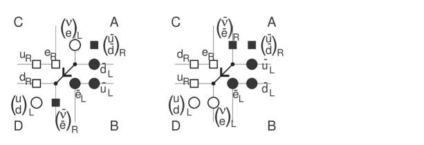
Figure 3: Assignment of first-generation fermions for ${\mathfrak{vle}}(3|6)$ (left) and ${\mathfrak{mb}}(3|8)$ (right). White = particles and black = anti-particles. Circles = left-handed and squares = right-handed. The arrows in the middle indicate the overall direction of the morphisms, and the sectors are labelled as in Figure 1.

It is quite remarkable that it is possible to fit the $sl(3)\!\oplus\!sl(2)$ weights of all fundamental fermions so snugly in the list of form modules. It is e.g. not at all possible to identify the $sl(3)$ gauge bosons with forms, due to the $(1,1)$ $sl(3)$ weight. On other hand, we know that the gauge bosons must be connections, so identifying them with form modules is out of the question anyway. However, not all $gl(1)$ weights come out correctly. ${\mathfrak{vle}}(3|6)$ predicts that the right-handed u quark $u_{R}$ should have $z=-8$, which disagrees with the correct value $z=4$ $(Y=4/3)$ by two units of hypercharge. Similarly, the left-handed u anti-quark $\tilde{u}_{L}$ has $z=8$ versus the correct $z=-4$. For ${\mathfrak{mb}}(3|8)$ the discrepancy is even bigger, but here the error in $z$ is constant in each of the four sectors:

$$\begin{array}[]{c|cccc}&A&B&C&D\\ \hline\cr\Delta z&-6&-18&+12&0\\ \end{array}$$

Upon second quantization, the ${\mathfrak{g}}_{0}$-invariant fermions in the standard model become field operators which satisfy the Clifford algebra

$$\{\bar{\psi}(x),\psi(x^{\prime})\}=\delta^{N}(x-x^{\prime}).$$ (5.152)

Similarly, we assume that the ${\mathfrak{g}}$-invariant fermions satisfy the Clifford algebra

$$\{\bar{\psi}(x,y),\psi(x^{\prime},y^{\prime})\}=\delta^{N}(x-x^{\prime})\delta^{n|m}(y-y^{\prime}).$$ (5.153)

Elimination of the second delta function requires precisely one integration over internal space. The simplest way to relate (5.152) and (5.153) is to put

$$\psi(x)=\psi(x,y_{0}),\qquad\bar{\psi}(x)=\int d^{n|m}\!y\,\bar{\psi}(x,y),$$ (5.154)

where $y_{0}$ is a constant, because $\int d^{n|m}\!y\,\delta^{n|m}(y-y_{0})=1$. For ${\mathfrak{mb}}(3|8)$, this integral adds $+6$ to the weight for the anti-fermions, which leaves us with the following errors:

$$\begin{array}[]{c|cccc}&A&B&C&D\\ \hline\cr\Delta z&0&-12&+12&0\\ \end{array}$$ (5.157)

For ${\mathfrak{vle}}(3|6)$ the volume form has weight zero (${\mathfrak{vle}}(3|6)$ vector fields are divergence free), so integration does not change hypercharge.

It is more difficult to reconcile the values of $z$ in sector C, but this problem could be related to the “wedge product”, i.e. the mapping of a pair of form modules into a new one. In the D sector, we can define a map in the natural way:

$$\wedge: \Omega_{D}(q,r)\otimes\Omega_{D}(q^{\prime},r^{\prime})\longrightarrow\Omega_{D}(q+q^{\prime},r+r^{\prime})$$

$$f(y)\bar{\gamma}_{i_{1}a_{1}}...\bar{\gamma}_{i_{q}a_{q}}\bar{\beta}_{a_{q+1}}...\bar{\beta}_{a_{r}}\otimes g(y)\bar{\gamma}_{j_{1}b_{1}}...\bar{\gamma}_{j_{q^{\prime}}b_{q^{\prime}}}\bar{\beta}_{b_{q^{\prime}+1}}...\bar{\beta}_{b_{r^{\prime}}}\mapsto$$

$$\mapsto f(y)g(y)\bar{\gamma}_{i_{1}a_{1}}...\bar{\gamma}_{i_{q}a_{q}}\bar{\gamma}_{j_{1}b_{1}}...\bar{\gamma}_{j_{q^{\prime}}b_{q^{\prime}}}\bar{\beta}_{a_{q+1}}...\bar{\beta}_{a_{r}}\bar{\beta}_{b_{q^{\prime}+1}}...\bar{\beta}_{b_{r^{\prime}}}.$$

In terms of ${\mathfrak{g}}_{0}$ weights,

$$\wedge: (0,q;r;4q-3r)\otimes(0,q^{\prime};r^{\prime};4q^{\prime}-3r^{\prime})\to$$

$$\to(0,q+q^{\prime};r+r^{\prime};4(q+q^{\prime})-3(r^{\prime}+r^{\prime})).$$

However, the wedge product in the C sector must be defined by

$$\wedge: (0,q;r;4q+3r+6)\otimes(0,q^{\prime};r^{\prime};4q^{\prime}+3r^{\prime}+6)\to$$

$$\to(0,q+q^{\prime};r+r^{\prime};4(q+q^{\prime})+3(r^{\prime}+r^{\prime})+6).$$

The total value of $z$ is $(4q+3r+6)+(4q^{\prime}+3r^{\prime}+6)$ to the left but only $4(q+q^{\prime})+3(r^{\prime}+r^{\prime})+6$ to the right; six units of $z$ (i.e. two units of hypercharge) have been “eaten” by the wedge product. A reasonable conclusion is that the interpretation of the value of $z$ in the C sector is unclear. It might be possible to add an overall multiple of $6$, but this multiple should be the same for all modules in the sector. After addition of $\Delta z=-12$ to the C sector (and $\Delta z=+12$ to the B sector), the hypercharge assignments agree with the standard model.

Suitable wedge products can be defined in other sectors similarly; the wedge product between forms from different sectors involves contraction of dual indices. The wedge product appears in Figure 1 simply as vector addition; associativity and graded commutativity follows immediately because vector addition has these properties. There is some ambiguity when the results ends on some of the coordinate axes, since then there are two different form modules with different value of $z$. It is remarkable that the fundamental fermions in the first generation are exactly right to make it possible to build all form modules from wedge products. It might appear from Figure 3 that there are too many fermions, but we must keep in mind that the fermions are spinors as well, so there is an extra quantum number due to spin.

A ${\mathfrak{g}}_{0}$ gauge theory is symmetric under interchange of particles and anti-particles, but not the ${\mathfrak{g}}$ theory. In Figure 3, CP amounts to a reflection in the origin, but the direction of the morphisms (indicated by the diagonal arrow) is unchanged. To obtain complete reflection, we must also reverse the direction of all morphisms, which can be interpreted as time reversal T. Thus CPT is conserved, at least in this figure, but CP and T are manifestly broken. Note the difference to the standard model, where breaking of CP is dynamical but not manifest. The inequivalence of dual modules is completely analogous to the difference between contravariant and covariant tensors: conventional in $gl(N)$, but substantial in ${\mathfrak{vect}}(N)$. Only covariant skew tensor fields admit a morphism, the exterior derivative.

Despite the fact that ${\mathfrak{vle}}(3|6)$ and ${\mathfrak{mb}}(3|8)$ are superalgebras, it seems that no supersymmetric partners arise in the second-gauged theories. The multiplets have both bosonic and fermionic components, but the weights are the same as for $sl(3)\!\oplus\!sl(2)\!\oplus\!gl(1)$ and only the lowest-weight states are identified with particles. However, this point requires further study.

We have identified fermions in the first generation with form modules. What about the second and third generations? Since later generations have the same quantum numbers as the first, the natural thing is to combine several generations, i.e. ${\mathfrak{g}}_{0}$ modules, into a single ${\mathfrak{g}}$ module. However, the decomposition of the ${\mathfrak{g}}$ form modules into irreducible ${\mathfrak{g}}_{0}$ modules has not yet been studied.

All considerations in this paper are classical. Quantization of a second-gauged theory will presumably encounter problems similar to those in quantum gravity. On the mathematical side, the construction of Fock modules with the normal ordering prescription gives rise to a higher-dimensional generalization of the Virasoro algebra; such modules were first constructed for ${\mathfrak{vect}}(N)$ by Rao and Moody [24] and in the super case by myself [16]. It is clear that every vectorial Lie superalgebra ${\mathfrak{g}}\subset{\mathfrak{vect}}(n|m)$ have similar Fock representations; the geometrical construction in [17] goes through also for superalgebras. However, ordinary quantization methods only work when the symmetry algebras have no or possibly central extensions, and the Virasoro-like cocycle is non-central except for algebras of linear growth.

We conclude with a summary of the main features and predictions of the second-gauged standard model based on ${\mathfrak{mb}}(3|8)$:

1. All fermions in the first generation can be identified with closed form modules, but the assignment of hypercharge is unclear, maybe wrong.

2. All closed form modules can be built by taking suitably defined wedge products of the fundamental fermions.

3. The gauge bosons acquire more components, but there are still only $\dim{\mathfrak{g}}_{0}=12$ different types.

4. There are presumably no supersymmetric partners, since irreducible ${\mathfrak{g}}$ modules, and hence fundamental particles, are labelled by ${\mathfrak{g}}_{0}$ weights.

5. The symmetry between particles and anti-particles is manifestly broken.

6. Several generations might arise by decomposing ${\mathfrak{g}}$ irreps into ${\mathfrak{g}}_{0}$ irreps.

7. The internal space must be combined with spacetime, but internal directions are nevertheless fundamentally different from the spacetime directions.

Although there are shortcomings, in particular concerning the unclear assignment of hypercharge, I believe that this list is sufficiently close to experimental data to merit further study of the second-gauged standard model.

References

[1] Alekseevsky D., Leites D., Shchepochkina I.:
Examples of simple Lie superalgebras of vector fields.
C. R. Acad. Bulg. Sci., 34 1187–1190, (1980) (in Russian)
[2] Bernstein J. and Leites, D.:
Invariant differential operators and irreducible representations
of Lie superalgebras of vector fields.
Sel. Math. Sov. 1 143–160 (1981)
[3] Cartan, E.:
Les groupes des transformations continués, infinis, simples.
Ann. Sci. Ecole Norm. Sup. 26, 93–161 (1909)
[4] Cheng, S.-J. and Kac, V.G.:
A new superconformal algebra.
Comm. Math. Phys. 186, 219–231 (1997)
[5] Cheng, S.-J. and Kac, V.G.:
Structure of some -graded Lie superalgebras of vector
fields.
Transformation groups 4, 219–272 (1999)
[6]
Grozman, P., Leites, D. and Shchepochkina, I.:
Invariant operators on supermanifolds and standard models.
In: M. Olshanetsky and A. Vainshtein (eds.)
Multiple facets of quantization and supersymmetry,
Michael Marinov Memorial Volume, World Sci., to appear. ESI preprint 1111, www.esi.ac.at
[7] Günaydin, M., Koepsell, K., and Nicolai, H.:
Conformal and quasiconformal realizations of exceptional Lie groups.
Commun. Math. Phys. 221, 57–76 (2001)
[8] Huang, K.:
Quarks, leptons and gauge fields, 2nd ed.
World Scientific (1986)
[21]
Leites, D. and Shchepochkina, I.:
Towards classification of simple vectorial Lie superalgebras.
In Leites D. (ed.):
Seminar on Supermanifolds, Reports of Stockholm University,
30/1988-13 and 31/1988-14 (1988)
[22]
Leites, D. and Shchepochkina, I.:
Classification of the simple Lie superalgebras of vector fields.
Preprint (2000)
[23] Leites, D.:
Toward classification of classical Lie superalgebras.
In: Nahm Z., Chau L. (eds.) Differential geometric methods in
theoretical physics,
(Davis, CA, 1988), NATO Adv. Sci. Inst. Ser. B Phys., 245,
Plenum, New York, 633–651 (1990)
[24] Rao, S.E. and Moody, R.V.:
Vertex representations for -toroidal Lie algebras and a
generalization of the Virasoro algebra.
Commun. Math. Phys. 159, 239–264 (1994)
[25] Shchepochkina, I.:
Exceptional simple infinite dimensional Lie superalgebras.
C. R. Acad. Bulg. Sci. 36, 313–314 (1983) (in Russian)
[26] Shchepochkina, I.:
The five exceptional simple Lie superalgebras of vector fields.
hep-th/9702121 (a preliminary version of [27])
[27] Shchepochkina, I.:
Five exceptional simple Lie superalgebras of vector fields and
their fourteen regradings.
Represent. Theory, 3, 373–415 (1999)
[28] Shchepochkina, I. and Post G.:
Explicit bracket in an exceptional simple Lie superalgebra.
Internat. J. Algebra Comput. 8, 479–495 (1998)
physics/9703022