Abstract

In this work we define and study the relations between Lorentzian manifolds given by the diffeomorphisms which map causal future directed vectors onto causal future directed vectors. This class of diffeomorphisms, called proper causal relations, contains as a subset the well-known group of conformal relations and are deeply linked to the so-called causal tensors of Ref.[1]. If two given Lorentzian manifolds are in mutual proper causal relation then they are said to be causally isomorphic: they are indistinguishable from the causal point of view. Finally, the concept of causal transformation for Lorentzian manifolds is introduced and its main mathematical properties briefly investigated.

1 Basics on causal relations

In this section the definitions of the basic concepts and the notation to be used throughout this contribution shall be presented. Differentiable manifolds are denoted by italic capital letters $\it V,W,U,\dots$ and, to our purposes, all such manifolds will be connected causally orientable Lorentzian manifolds of dimension $\it n$. The signature convention is set to $(+-\dots-)$. $T_{x}(V)$ and $T^{*}_{x}(V)$ will stand respectively for the tangent and cotangent spaces at $x\in V$, and $T(\it V)$ (resp. $T^{*}(\it V)$) is the tangent bundle (cotangent bundle) of $\it V$. Similarly the bundle of $j$-contravariant and $k$-covariant tensors of $V$ is denoted ${\cal T}^{j}_{k}(V)$. If $\varphi$ is a diffeomorphism between $V$ and $W$, the push-forward and pull-back are written as $\varphi^{{}^{\prime}}$ and $\varphi^{*}$ respectively. The hyperbolic structure of the Lorentzian scalar product naturally splits the elements of $T_{x}(V)$ into timelike, spacelike, and null, and as usual we use the term causal for the vectors (or vector fields) which are non-spacelike. To fix the notation we introduce the sets:

$$\Theta^{+}(x) = \{\vec{X}\in T_{x}(V):\vec{X}\ \mbox{is causal future directed}\},$$

$$\Theta(x) = \Theta^{+}(x)\cup\Theta^{-}(x),\hskip 28.45274pt\Theta^{+}(V)=\bigcup_{x\in V}\Theta^{+}(x)$$

with obvious definitions for $\Theta^{-}(x)$, $\Theta^{-}(V)$ and $\Theta(V)$. Before we proceed, we need to introduce a further concept taken from [1].

Definition 1.1

A tensor ${\bf T}\in{\cal T}^{0}_{r}(x)$ satisfies the dominant property if for every $\vec{k}_{1},\dots,\vec{k}_{r}\in\Theta^{+}(x)$ we have that ${\bf T}(\vec{k}_{1},\dots,\vec{k}_{r})\geq 0$.

The set of all $r$-tensors with the dominant property at $x\in V$ will be denoted by ${\cal DP}^{+}_{r}(x)$ whereas ${\cal DP}^{-}_{r}(x)$ is the set of tensors such that $-{\bf T}\in{\cal DP}^{+}_{r}(x)$. We put ${\cal DP}_{r}(x)\equiv{\cal DP}^{+}_{r}(x)\cup{\cal DP}^{-}_{r}(x)$. All these definitions extend straightforwardly to the bundle ${\cal T}^{0}_{r}(V)$ and we may define the subsets ${\cal DP}^{+}_{r}({\cal U})$, ${\cal DP}^{-}_{r}({\cal U})$ and ${\cal DP}_{r}({\cal U})$ for an open subset ${\cal U}\subseteq V$ as follows:

$${\cal DP}^{\pm}_{r}(U)=\bigcup_{x\in{\cal U}}{\cal DP}^{\pm}_{r}(x),\,\,\,{\cal DP}_{r}({\cal U})={\cal DP}^{+}_{r}({\cal U})\cup{\cal DP}^{-}_{r}({\cal U}).$$

The simplest example (leaving aside $\mathbb{R}^{+}$) of causal tensors are the causal 1-forms ($\equiv{\cal DP}_{1}(V)$) [1], while a general characterization of ${\cal DP}^{+}_{r}\equiv{\cal DP}^{+}_{r}(V)$ is the following (see [2] for a proof)¹:

Proposition 1.1

${\bf T}\in{\cal DP}^{+}_{r}$ if and only if the components $T_{i_{1}\dots i_{r}}$ of ${\bf T}$ in all orthonormal bases fulfill $T_{0\dots 0}\geq|T_{i_{1}\dots i_{r}}|$, $\forall i_{1}\dots i_{r}$, where the $0$-index refers to the temporal component.

We are now ready to present our main concept, which tries to capture the notion of some kind of relation between the causal structure of $V$ and $W$.

Definition 1.2

Let $\varphi:V\rightarrow W$ be a global diffeomorphism between two Lorentzian manifolds. We shall say that $W$ is properly causally related with $V$ by $\varphi$, denoted $V\prec_{\varphi}W$, if for every $\vec{X}\in\Theta^{+}(V)$ we have that $\varphi^{{}^{\prime}}\vec{X}$ belongs to $\Theta^{+}(W)$. $W$ is said to be properly causally related with $V$, denoted simply as $V\prec W$, if $\exists\varphi$ such that $V\prec_{\varphi}W$.

Remarks

1. This definition can also be given for any set $\zeta\subseteq V$ by demanding that $(\varphi^{{}^{\prime}}\vec{X})_{\varphi(x)}\in\Theta^{+}(\varphi(x))\,\,\,\,\forall\vec{X}\in\Theta^{+}(x)$, $\forall x\in\zeta$.

2. Two diffeomorphic Lorentzian manifolds may fail to be properly causally related as we shall show later with explicit examples.

Definition 1.3

Two Lorentzian manifolds $V$ and $W$ are called causally isomorphic if $V\prec W$ and $W\prec V$. This shall be written as $V\sim W$.

We claim that if $V\sim W$ then their causal structure are somehow the same.

Let ${\bf g}$ and $\tilde{{\bf g}}$ be the Lorentzian metrics of $V$ and $W$ respectively. By using

$$\tilde{{\bf g}}(\varphi^{{}^{\prime}}\vec{X},\varphi^{{}^{\prime}}\vec{Y})=\varphi^{*}\tilde{{\bf g}}(\vec{X},\vec{Y}),$$ (1)

we immediately realize that $V\prec_{\varphi}W$ implies that $\varphi^{*}\tilde{{\bf g}}\in{\cal DP}^{+}_{2}(V)$. Conversely, if $\varphi^{*}\tilde{{\bf g}}\in{\cal DP}^{+}_{2}(V)$ then for every $\vec{X}\in\Theta^{+}(V)$ we have that $(\varphi^{*}\tilde{{\bf g}})(\vec{X},\vec{X})=\tilde{{\bf g}}(\varphi^{{}^{\prime}}\vec{X},\varphi^{{}^{\prime}}\vec{X})\geq 0$ and hence $\varphi^{{}^{\prime}}\vec{X}\in\Theta(W)$. However, it can happen that $\Theta^{+}(V)$ is actually mapped to $\Theta^{-}(W)$, and $\Theta^{-}(V)$ to $\Theta^{+}(W)$. This only means that $W$ with the time-reversed orientation is properly causally related with $V$. Keeping this in mind, the assertion $\varphi^{*}\tilde{{\bf g}}\in{\cal DP}^{+}_{2}(V)$ will be henceforth taken as equivalent to $V\prec_{\varphi}W$.

2 Mathematical properties

Let us present some mathematical properties of proper causal relations.

Proposition 2.1

If $V\prec_{\varphi}W$ then:

1. $\vec{X}\in\Theta^{+}(V)$ is timelike $\Longrightarrow$ $\varphi^{{}^{\prime}}\vec{X}\in\Theta^{+}(W)$ is timelike.

2. $\vec{X}\in\Theta^{+}(V)$ and $\varphi^{{}^{\prime}}\vec{X}\in\Theta^{+}(W)$ is null $\Longrightarrow$ $\vec{X}$ is null.

Proof :    For the first implication, if $\vec{X}\in\Theta^{+}(V)$ is timelike we have, according to equation (1), that $\varphi^{*}\tilde{{\bf g}}(\vec{X},\vec{X})=\tilde{{\bf g}}(\varphi^{{}^{\prime}}\vec{X},\varphi^{{}^{\prime}}\vec{X})$ which must be a strictly positive quantity as $\varphi^{*}\tilde{{\bf g}}\in{\cal DP}^{+}_{2}(W)$ [1]. For the second implication, equation (1) implies $0=\varphi^{*}\tilde{{\bf g}}(\vec{X},\vec{X})$ which is only possible if $\vec{X}$ is null since $\varphi^{*}\tilde{{\bf g}}\in{\cal DP}^{+}_{2}(V)$ and $\vec{X}\in\Theta^{+}(V)$ (see again [1]).  

Proposition 2.2

$V\prec_{\varphi}W\hskip 5.69054pt\Longleftrightarrow\hskip 5.69054pt\varphi^{{}^{\prime}}\vec{X}\in\Theta^{+}(W)$ for all null $\vec{X}\in\Theta^{+}(V)$.

Proof :    For the non-trivial implication, making again use of (1) we can write:

$$\varphi^{{}^{\prime}}\vec{X}\in\Theta^{+}(W)\ \forall\vec{X}\ \mbox{null in}\ \Theta^{+}(V)\Leftrightarrow\varphi^{*}\tilde{{\bf g}}(\vec{X},\vec{Y})\geq 0\ \ \forall\ \vec{X},\vec{Y}\ \mbox{null in}\ \Theta^{+}(V)$$

which happens if and only if $\varphi^{*}\tilde{{\bf g}}$ is in ${\cal DP}^{+}_{2}(V)$ (see [1] property 2.4).  

Proposition 2.3 (Transitivity of the proper causal relation)

If $V\prec_{\varphi}W$ and $W\prec_{\psi}U$ then $V\prec_{\psi\circ\varphi}U$

Proof :    Consider any $\vec{X}\in\Theta^{+}(V)$. Since $V\prec_{\varphi}W$, $\varphi^{{}^{\prime}}\vec{X}\in\Theta^{+}(W)$ and since $W\prec_{\psi}U$ we get $\psi^{{}^{\prime}}[\varphi^{{}^{\prime}}\vec{X}]\in\Theta^{+}(U)$ so that $(\psi\circ\varphi)^{{}^{\prime}}\vec{X}\in\Theta^{+}(U)$ from what we conclude that $V\prec_{\psi\circ\varphi}U$.  

Therefore, we see that the relation $\prec$ is a preorder. Notice that if $V\sim W$ (that is $V\prec W$ and $W\prec V$) this does not imply that $V=W$. Nevertheless, one can always define a partial order for the corresponding classes of equivalence.

Next, we identify the part of the boundary of the null cone which is preserved under a proper causal relation. A lemma is needed first. Recall that $\vec{X}$ is called an “eigenvector” of a 2-covariant tensor ${\bf T}$ if ${\bf T}(\cdot,\vec{X})=\lambda{\bf g}(\cdot,\vec{X})$ and $\lambda$ is then the corresponding eigenvalue.

Lemma 2.1

If ${\bf T}\in{\cal DP}^{+}_{2}(x)$ and $\vec{X}\in\Theta^{+}(x)$ then ${\bf T}(\vec{X},\vec{X})=0\ \Longleftrightarrow\vec{X}$ is a null eigenvector of ${\bf T}$.

Proof :    Let $\vec{X}\in\Theta^{+}(x)$ and assume $0={\bf T}(\vec{X},\vec{X})=T_{ab}X^{a}X^{b}$. Then since $T_{ab}X^{b}\in{\cal DP}^{+}_{1}(x)$ [1] we can conclude that $X_{a}$ and $T_{ab}X^{b}$ must be proportional which results in $X^{a}$ being a null eigenvector of $T_{ab}$. The converse is straightforward.  

Proposition 2.4

Assume that $V\prec_{\varphi}W$ and $\vec{X}\in\Theta^{+}(x),\ x\in V$. Then $\varphi^{{}^{\prime}}\vec{X}$ is null at $\varphi(x)\in W$ if and only if $\vec{X}$ is a null eigenvector of $\varphi^{*}\tilde{{\bf g}}(x)$.

Proof :    Let $\vec{X}$ be in $\Theta^{+}(x)$ and suppose $\varphi^{{}^{\prime}}\vec{X}$ is null at $\varphi(x)$. Then, according to proposition 2.1, $\vec{X}$ is also null at $x$. On the other hand we have $0=\tilde{{\bf g}}(\varphi^{{}^{\prime}}\vec{X},\varphi^{{}^{\prime}}\vec{X})=\varphi^{*}\tilde{{\bf g}}(\vec{X},\vec{X})$ and since $\varphi^{*}\tilde{{\bf g}}|_{x}\in{\cal DP}^{+}_{2}(x)$, lemma 2.1 implies that $\vec{X}$ is a null eigenvector of $\varphi^{*}\tilde{{\bf g}}$ at $x$.  

The vectors which remain null under the causal relation $\varphi$ are called its canonical null directions. On the other hand, the null eigenvectors of ${\bf T}\in{\cal DP}^{+}_{2}$ can be used to classify this tensor, as proved in [1]. As a result we have

Proposition 2.5

If the relation $V\prec_{\varphi}W$ has n linearly independent canonical null directions then $\varphi^{*}\tilde{{\bf g}}=\lambda{\bf g}$.

Proof :    If there exist $n$ independent canonical null directions, then $\varphi^{*}\tilde{{\bf g}}$ has $n$ independent null eigenvectors which is only possible if $\varphi^{*}\tilde{{\bf g}}$ is proportional to the metric tensor ${\bf g}$ ([1, 2].)  

Proposition 2.5 has an interesting application in the following theorem

Theorem 2.1

Suppose that $V\prec_{\varphi}W$ and $W\prec_{\varphi^{-1}}V$. Then $\varphi^{*}\tilde{{\bf g}}=\lambda{\bf g}$ and $(\varphi^{-1})^{*}{\bf g}=\frac{1}{(\varphi^{-1})^{*}\lambda}\tilde{{\bf g}}$ for some positive function $\lambda$ defined on $V$.

Proof :    Under these hypotheses, using proposition 2.1, we get the following intermediate results

$$\varphi^{{}^{\prime}}\vec{X}\in\Theta^{+}(W)\ \mbox{null and $\vec{X}\in\Theta^{+}(V)$}\Longrightarrow\vec{X}\ \mbox{is null,}$$

$$(\varphi^{-1})^{{}^{\prime}}\vec{Y}\in\Theta^{+}(V)\ \mbox{null and $\vec{Y}\in\Theta^{+}(W)$}\Longrightarrow\vec{Y}\ \mbox{is null.}$$

Now, let $\vec{X}\in\Theta^{+}(V)$ be null and consider the unique $\vec{Y}\in T(V)$ such that $\vec{X}=(\varphi^{-1})^{{}^{\prime}}\vec{Y}$. Then $\vec{Y}=\varphi^{{}^{\prime}}\vec{X}$ and $\vec{Y}\in\Theta^{+}(W)$ as $\varphi$ sets a proper causal relation and $\vec{X}$ is in $\Theta^{+}(V)$. Hence, according to the second result above $\vec{Y}$ must be null and we conclude that every null $\vec{X}\in\Theta^{+}(V)$ is push-forwarded to a null vector of $\Theta^{+}(W)$ which in turn implies that $\varphi^{*}\tilde{{\bf g}}=\lambda{\bf g}$. In a similar fashion, we can prove that $(\varphi^{-1})^{*}{\bf g}=\mu\tilde{{\bf g}}$ and hence $(\varphi^{-1})^{*}\lambda=1/\mu$.  

Corollary 2.1

$V\prec_{\varphi}W$ and $W\prec_{\varphi^{-1}}V\,\,\Longleftrightarrow\,\,\varphi$ is a conformal relation.

3 Applications to causality theory

In this section we will perform a detailed study of how two Lorentzian ma-
nifolds $V$ and $W$ such that $V\prec_{\varphi}W$ share common causal features. To begin with, we must recall the basic sets used in causality theory, namely $I^{\pm}(p)$ and $J^{\pm}(p)$ for any point $p\in V$ (these definitions can also be given for sets). One has $q\in J^{+}(p)$ (respectively $q\in I^{+}(p)$) if there exists a continuous future directed causal (resp. timelike) curve joining $p$ and $q$. Recall also the Cauchy developments $D^{\pm}(\zeta)$ for any set $\zeta\subseteq V$ [3, 4, 5]. Another important concept is that of future set: $\mbox{A}\subset V$ is said to be a future set if $I^{+}(\mbox{A})\subseteq\mbox{A}$. For example $I^{+}(\zeta)$ is a future set for any $\zeta$. All these concepts are standard in causality theory and are defined in many references, see for instance [3, 4, 5].

Proposition 3.1

If $V\prec_{\varphi}W$ then, for every set $\zeta\subseteq V$, we have $\varphi(I^{\pm}(\zeta))\subseteq I^{\pm}(\varphi(\zeta))$ and $\varphi(J^{\pm}(\zeta))\subseteq J^{\pm}(\varphi(\zeta))$.

Proof :    It is enough to prove it for a single point $p\in V$ and then getting the result for every $\zeta$ by considering it as the union of its points. For the first relation, let $y$ be in $\varphi(I^{+}(p))$ arbitrary and take $x\in I^{+}(p)$ such that $\varphi(x)=y$. Choose a future-directed timelike curve $\gamma$ joining $p$ and $x$. From proposition 2.1, $\varphi(\gamma)$ is then a future-directed timelike curve joining $\varphi(p)$ and $y$, so that $y\in I^{+}(\varphi(p))$. The second assertion is proven in a similar way using again proposition 2.1. The proof for the past sets is analogous.  

The converse of this proposition does not hold in general unless we impose some causality conditions on the spacetime.

Definition 3.1

A Lorentzian manifold $V$ is said to be distinguishing if for every neighbourhood $U_{p}$ of $p\in V$ there exist another neighbourhood $B_{p}\subset U_{p}$ containing $p$ which intersects every causal curve meeting $p$ in a connected set.

We need some concepts of standard causality theory. For any $p\in V$ one can introduce normal coordinates in a neighbourhood ${\cal N}_{p}$ of $p$ (see, e.g. [5]). Then the exponential map provides a diffeomorphism $\exp:{\cal O}\subset T_{p}(V)\rightarrow{\cal N}_{p}$ where ${\cal O}$ is an open neighbourhood of $\vec{0}\in T_{p}(V)$. The interior of the future (past) light cone of $p$ is defined by $C^{\pm}_{p}=\exp(\mbox{int}(\Theta^{\pm}(p))\cap{\cal O})$, and obviously $C^{\pm}_{p}\subseteq I^{\pm}(p)$ [5]. Other important issue deals with the chronology relation $<\!\!<$ between two points. We have $p<\!\!<q$ if there exist a future timelike curve joining $p$ and $q$. See [6] for an axiomatic study of this relation.

Proposition 3.2

Let $\gamma$ be a piecewise continuous curve of a distinguishing Lorentzian manifold $(V,{\bf g})$. Then, $\gamma$ is total with respect to $<\!\!<$ if and only if $\gamma$ is timelike.

Proof :    Clearly if $\gamma$ is timelike then $\gamma$ must be a total set for the relation $<\!\!<$ (this is true for every spacetime). For the converse consider a curve $\gamma$ which is total with respect to $<\!\!<$ and let $q\in\gamma$ be an arbitrary point of the curve. If we take a normal neighbourhood of $q$, ${\cal N}_{q}$ then we can find a neighbourhood $U_{q}$ of $q$ which is intersected in a connected set by every causal curve meeting $q$. Now, if we pick up a point $z\in\gamma\cap U_{q}$ we have that either $q<\!\!<z$ or $z<\!\!<q$. Assuming the former we deduce that there exists a timelike curve $\tilde{\gamma}$ joining $q$ and $z$ which implies that $\tilde{\gamma}\cap U_{q}$ is a connected set. This property together with the distinguishability of $V$ implies that $\tilde{\gamma}$ must be a subset of $U_{q}$ and hence $\tilde{\gamma}\subset{\cal N}_{q}$ from what we conclude that $\tilde{\gamma}\subset C_{p}$ ([5]) and hence $z\in C_{p}$ $\forall z\in\gamma\cap U_{q}$ which is only possible if $\gamma\cap U_{q}$ is timelike. By covering $\gamma$ with sets of the form $\gamma\cap U_{q}$, $q\in\gamma$ we arrive at the desired result.  

Proposition 3.3

Let $\varphi:V\rightarrow W$ be a diffeomorphism with the property $\varphi(I^{+}(p))\subseteq I^{+}(\varphi(p))\ \forall p\in V$. Then if $W$ is distinguishing, $\varphi$ is a proper causal relation. A similar result holds replacing $I^{+}$ by $I^{-}$.

Proof :    From the statement of this proposition is clear that $\forall$ $p,q$ of $V$ such that $p<\!\!<q$ then $\varphi(p)<\!\!<\varphi(q)$. Therefore every timelike curve $\gamma$ of $V$ is mapped onto a continuous curve in $W$ total with respect to $<\!\!<$ and hence timelike due to the distiguishability of $W$. Furthermore if the curve $\gamma$ is future directed then $\varphi(\gamma)$ must be also future directed since $<\!\!<$ is preserved which is only possible if every timelike future-pointing vector is mapped onto a future-pointing timelike vector. As a consequence, if $\vec{k}$ is a null vector, $\varphi^{{}^{\prime}}\vec{k}$ must be a causal vector (to see it just construct a sequence of timelike future directed vectors converging to $\vec{k}$) which proves that $\varphi$ is a proper causal relation.  

The results for the Cauchy developments are the following:

Proposition 3.4

If $V\prec_{\varphi}W$ then $D^{\pm}(\varphi(\zeta))\subseteq\varphi(D^{\pm}(\zeta)),\,\,\forall\zeta\subseteq V$.

Proof :    It is enough to prove the future case. Let $y\in D^{+}(\varphi(\zeta))$ arbitrary and consider any causal past directed curve $\gamma^{-}_{\varphi^{-1}(y)}\subset V$ containing $\varphi^{-1}(y)$. Since the image curve by $\varphi$ of $\gamma^{-}_{\varphi^{-1}(y)}$ is a causal curve passing through $y$, ergo meeting $\varphi(\zeta)$, we have that $\gamma^{-}_{\varphi^{-1}(y)}$ must meet $\zeta$ from what we conclude that $y\in\varphi(D^{+}(\zeta))$ due to the arbitrariness of $\gamma^{-}_{\varphi^{-1}(y)}$.  

Corollary 3.1

If $\Sigma\subset W$ is a Cauchy hypersurface then $\varphi^{-1}(\Sigma)$ is also a Cauchy hypersurface of $V$.

Proof :    If $\Sigma$ is a Cauchy hypersurface then $D(\Sigma)=W$, and from proposition 3.4 $D(\Sigma)\subseteq\varphi(D(\varphi^{-1}(\Sigma)))$. Since $\varphi$ is a diffeomorphism the result follows.  

One can prove the impossibility of the existence of proper causal relations sometimes. For instance, from the previous corollary we deduce that $V\prec W$ is impossible if $W$ is globally hyperbolic but $V$ is not. Other impossibilities arise as follows. Let us recall that, for any inextendible causal curve $\gamma$, the boundaries $\partial I^{\pm}(\gamma)$ of its chronological future and past are usually called its future and past event horizons, sometimes also called particle horizons [3, 4, 5]. Of course these sets can be empty (then one says that $\gamma$ has no horizon).

Proposition 3.5

Suppose that every inextendible causal future directed curve in $W$ has a non-empty $\partial I^{-}(\gamma)$ ($\partial I^{+}(\gamma)$). Then any V such that $V\prec W$ cannot have inextendible causal curves without past (future) event horizons.

Proof :    If there were a future-directed curve $\gamma$ in $V$ with $\partial I^{-}(\gamma)=\emptyset$, $I^{-}(\gamma)$ would be the whole of $V$. But according to proposition 3.1 $\varphi(I^{-}(\gamma))\subseteq I^{-}(\varphi(\gamma))$ from what we would conclude that $I^{-}(\varphi(\gamma))=W$ against the assumption.  

The class of future (or past) sets characterize the proper causal relations for distinguishing spacetimes as it is going to be shown next (every statement for future objects has a counterpart for the past).

Lemma 3.1

If A is a future set then $p\in\overline{\mbox{A}}\Longleftrightarrow I^{+}(p)\subseteq\mbox{A}$.

Proof :    Suppose $I^{+}(p)\subseteq A$. Then since $C_{p}^{+}\subseteq I^{+}(p)$ and $p\in\overline{C_{p}^{+}}$ we have that $U_{p}\cap C_{p}^{+}\neq\emptyset$ for every neighbourhood $U_{p}$ of $p$ which in turn implies that $U_{p}\cap\mbox{A}\neq\emptyset$ and hence $p\in\overline{\mbox{A}}$. Conversely, let $p$ be any point of $\overline{\mbox{A}}$ then $I^{+}(p)\subseteq I^{+}(\overline{A})=I^{+}(A)\subseteq A$.  

Theorem 3.1

Suppose that $(W,\tilde{{\bf g}})$ is a distinguishing spacetime. Then a diffeomorphism $\varphi:(V,{\bf g})\rightarrow(W,\tilde{{\bf g}})$ is a proper causal relation if and only if $\varphi^{-1}(\mbox{A})$ is a future set for every future set. $\mbox{A}\subseteq W$.

Proof :    Suppose $\mbox{A}\subseteq W$ is a future set, $V\prec_{\varphi}W$ and take $\varphi^{-1}(\mbox{A})\subseteq V$. Proposition 3.1 implies $\varphi(I^{+}(\varphi^{-1}(\mbox{A})))\subseteq I^{+}(\varphi(\varphi^{-1}(\mbox{A})))=I^{+}(\mbox{A})\subseteq\mbox{A}$ which shows that $I^{+}(\varphi^{-1}(\mbox{A}))\subseteq\varphi^{-1}(\mbox{A})$. Conversely, for any $p\in V$ take the future set $I^{+}(\varphi(p))$ and consider the future set $\varphi^{-1}(I^{+}(\varphi(p)))$. As $\varphi(p)\in\overline{I^{+}(\varphi(p))}$ then $p\in\overline{\varphi^{-1}(I^{+}(\varphi(p)))}$ and according to lemma 3.1 $I^{+}(p)\subseteq\varphi^{-1}(I^{+}(\varphi(p)))$ so that $\varphi(I^{+}(p))\subseteq I^{+}(\varphi(p))$. Since this holds for every $p\in V$ and $W$ is distinguishing, proposition 3.3 ensures that $\varphi$ is a proper causal relation.  

This theorem has important consequences.

Proposition 3.6

If $V\sim W$ and both manifolds are distinguishing, then there is a one-to-one correspondence between the future (and past) sets of $V$ and $W$.

Proof :    If $V\sim W$ then $V\prec_{\varphi}W$ and $W_{\prec\Psi}V$ for some diffeomorphisms $\varphi$ and $\Psi$. By denoting with ${\cal F}_{V}$ and ${\cal F}_{W}$ the set of future sets of $V$ and $W$ respectively, we have that $\varphi^{-1}({\cal F}_{W})\subseteq{\cal F}_{V}$ and $\Psi^{-1}({\cal F}_{V})\subseteq{\cal F}_{W}$, due to theorem 3.1. Since both $\varphi$ and $\Psi$ are bijective maps we conclude that ${\cal F}_{V}$ is in one-to-one correspondence with a subset of ${\cal F}_{W}$ and vice versa which, according to the equivalence theorem of Bernstein [7], implies that ${\cal F}_{V}$ is in one-to-one correspondence with ${\cal F}_{W}$.  

4 Causal transformations

In this section we will see how the concepts above generalize, in a natural way, the group of conformal transformations in a Lorentzian manifold $V$.

Definition 4.1

A transformation $\varphi:V\longrightarrow V$ is called causal if $V\prec_{\varphi}V$.

The set of causal transformations of $V$ will be denoted by ${\cal C}(V)$. This is a subset of the group of transformations of $V$ which is closed under the composition of diffeomorphisms, due to proposition 2.3, and contains the identity map. This algebraic structure is well-known, see e.g. [8], and called subsemigroup with identity or submonoid. Thus, ${\cal C}(V)$ is a submonoid of the group of diffeomorphisms of $V$. Nonetheless, ${\cal C}(V)$ usually fails to be a group. In fact we have,

Proposition 4.1

Every subgroup of causal transformations is a group of conformal transformations.

Proof :    Let $G\subseteq{\cal C}(V)$ be a subgroup of causal transformations and consider any $\varphi\in G$, so that both $\varphi$ and $\varphi^{-1}$ are causal transformations. Then $\varphi$ is necessarily a conformal transformation as follows from Theorem 2.1.  

From standard results, see [8], we know that ${\cal C}(V)\cap{\cal C}(V)^{-1}$ is just the group of conformal transformations of $V$ and there is no other subgroup of ${\cal C}(V)$ which contains ${\cal C}(V)\cap{\cal C}(V)^{-1}$. The causal transformations which are not conformal transformations are called proper causal transformations.

It is now a natural question whether one can define infinitesimal generators of one-parameter families of causal transformations which generalize the “conformal Killing vectors”, and in which sense. Notice, however, that if $\{\varphi_{s}\}_{s\in\mathbb{R}}$ is a one-parameter group of causal transformations, from the previous results the only possibility is that $\{\varphi_{s}\}$ be in fact a group of conformal motions. On the other hand, things are more subtle if there are no conformal transformations in the family $\{\varphi_{s}\}$ other than the identity, in which case it is easy to see that the ‘best’ one can accomplish is that either $G^{+}\equiv\{\varphi_{s}\}_{s\in\mathbb{R}^{+}}$ or $G^{-}\equiv\{\varphi_{s}\}_{s\in\mathbb{R}^{-}}$ is in ${\cal C}(V)$. If this happens one talks about maximal one-parameter submonoids of proper causal transformations. Of course, it is also possible to define local one-parameter submonoids of causal transformations $\{\varphi_{s}\}_{s\in I}$ for some interval $I=(-\epsilon,\epsilon)$ of the real line assuming that $\{\varphi_{s}\}_{s\in(0,\epsilon)}$ consists of proper causal transformations. In any of these cases, we can define the infinitesimal generator of $\{\varphi_{s}\}$ as the vector field $\vec{\xi}=d\varphi_{s}/ds|_{s=0}$. Given that $\varphi_{s}^{*}{\bf g}\in{\cal DP}_{2}$ for all $s\geq 0$ (or for all non-positive $s$), one can somehow control the Lie derivative of ${\bf g}$ with respect to $\vec{\xi}$. For instance, it is easy to prove that ${\pounds}_{\vec{\xi}}\,{\bf g}(\vec{k},\vec{k})\geq 0$ (or $\leq 0$) for all null $\vec{k}$, clearly generalizing the case of conformal Killing vectors. An explicit example of this will be shown in the next section.

5 Examples

Example 1 Einstein static universe and de Sitter spacetime. Let us take $V$ as the Einstein static universe [3] and $W=\SS$ as de Sitter spacetime. In both cases the manifold is $\mathbb{R}\times S^{3}$ and hence they are diffeomorphic. By proposition 3.5 we know that $V\not\prec W$ because every causal curve in de Sitter spacetime possesses event horizons. However, the proper causal relation in the opposite way does hold as can be shown by constructing it explicitly. The line element of each spacetime is (with the notation $d\Omega^{2}=d\theta^{2}+\sin^{2}\theta d\phi^{2}$):

$$V: ds^{2}=dt^{2}-a^{2}(d\chi^{2}+\sin^{2}\chi d\Omega^{2})\$$

$$W: d\tilde{s}^{2}=d\bar{t}^{2}-\alpha^{2}\cosh^{2}(\bar{t}/\alpha)(d\bar{\chi}^{2}+\sin^{2}\bar{\chi}d\bar{\Omega}^{2})\$$

where $\chi,\theta,\phi$ (and their barred versions) are standard coordinates in $S^{3}$ and $a,\alpha$ are constants. The diffeomorphism $\Psi:W\rightarrow V$ is chosen as $\{t=b\bar{t},\chi={\bar{\chi}},\theta={\bar{\theta}},\phi={\bar{\phi}}\}$ for a constant $b$. One can readily get $\Psi^{*}{\bf g}$

$$(\Psi^{*}{\bf g})_{ab}dx^{a}dx^{b}=b^{2}d\bar{t}^{2}-a^{2}(d\bar{\chi}^{2}+\sin^{2}\bar{\chi}d\bar{\Omega}^{2})$$

which on using proposition 1.1 shows that $\Psi^{*}{\bf g}\in{\cal DP}^{+}_{2}(W)$ if $b^{2}\geq a^{2}/\alpha^{2}$ and therefore $\Psi$ is proper causal relation for those $b$.

Example 2 Consider the following spacetimes: $\Lambda_{a}$ is the region of Lorentz-Minkowski spacetime with $R>a>0$ in spherical coordinates $\{T,R,\Theta,\Phi\}$; $W_{c}$ is the outer region of Schwarzschild spacetime with $r>c\geq 2M$ in Schwarzschild coordinates $\{t,r,\theta,\phi\}$. Define the diffeomorphism $\varphi:\Lambda_{a}\rightarrow W_{c}$ given by $\{t=bT,r=R-a+c,\theta=\Theta,\phi=\Phi\}$ for an appropriate positive constant $b$, so that we have

$$(\varphi^{*}\tilde{{\bf g}})_{ab}dx^{a}dx^{b}=b^{2}(1-\frac{2M}{R-a+c})dT^{2}-\frac{dR^{2}}{1-\frac{2M}{R-a+c}}-(R-a+c)^{2}d\Omega^{2}.$$

By choosing $b$ and $a$ one can achieve $\varphi^{*}\tilde{{\bf g}}\in{\cal DP}^{+}_{2}(V_{a})$ whenever $c>2M$, while for $c=2M$ $\varphi$ fails to be a proper causal relation. Actually $\Lambda_{a}\not\prec W_{2M}$ due to corollary 3.1 as $W_{2M}$ is globally hyperbolic but $\Lambda_{a}$ is not.

Take now the diffeomorphism $\Psi:W_{c}\rightarrow\Lambda_{a}$ defined by $\{T=t,R=r,\Theta=\theta,\Phi=\phi\}$, so that $\Psi^{*}{\bf g}$ reads $(\Psi^{*}{\bf g})_{ab}dx^{a}dx^{b}=dt^{2}-dr^{2}-r^{2}d{\Omega}^{2}$ from where we immediately deduce that $\Psi^{*}{\bf g}\in{\cal DP}^{+}_{2}(V)$ for every $c\geq 2M$ as long as $a\geq 2M$. We have thus proved that $W_{c}\sim\Lambda_{c}$ if $c>2M$, but not for $c=2M$. This is quite interesting and clearly related to the null character of the event horizon $r=2M$ in Schwarzschild’s spacetime.

Example 3 (Friedman cosmological models with $p=\gamma\rho$.) Let us take as $(W,\tilde{{\bf g}})$ the flat Friedman-Robertson-Walker (FRW) spacetimes in standard FRW coordinates $\{t,\chi,\theta,\phi\}$ with line element given by

$$ds^{2}=dt^{2}-a^{2}(t)(d\chi^{2}+\chi^{2}d\Omega^{2})$$

and assume that the source of Einstein’s equations is a perfect fluid with equation of state given by $p=\gamma\rho$ ($p=$ pressure, $\rho=$ density, $\gamma\in(-1,1)$ constant). Then the scale factor is $a(t)=Ct^{\frac{2}{3(1+\gamma)}}$ with constant $C$. By straightforward calculations, it can be proven the following causal equivalences:

$$W\sim\Lambda_{0}\ \mbox{for $\gamma=-1/3$ where $\Lambda_{0}$ is the whole Minkowski spacetime }$$

$$W\sim V\ \mbox{for $\gamma\neq-1/3$ where $(V,{\bf g})$ is the steady state part of $\SS$, \cite[cite]{[\@@bibref{}{FF}{}{}]}.}$$

These causal equivalences are rather intuitive if we have a look at the Penrose diagram of each spacetime (figure 1).

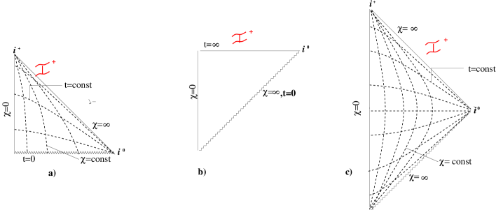
Figure 1: Penrose’s diagrams of FRW spacetimes for a) $-1/3<\gamma<1$ , b) $-1<\gamma<-1/3$ and c) $\gamma=1/3$. Notice the similar shape of diagram c) with that of $\Lambda$, and of the steady state part of $\SS$ with a) and b) [3].

Example 4 (Vaidya’s Spacetime.) Let us show finally an example of a submonoid of causal transformations. Consider the Vaidya spacetime whose line element is [9]

$$ds^{2}=\left(1-\frac{2M(t)}{r}\right)dt^{2}-2dtdr-r^{2}d\Omega^{2},\ \ -\infty<t<\infty,\ 0<r<\infty$$

where $t$ is a null coordinate (that is, $dt$ is a null 1-form), and $M(t)$ is a non-increasing function of $t$ interpreted as the mass. Take the diffeomorphisms $\varphi_{s}:t\mapsto t+s$. Then $\varphi^{*}_{s}{\bf g}$ can be cast in the form

$$\varphi^{*}_{s}{\bf g}={\bf g}-\frac{2}{r}(M(t+s)-M(t))dt\otimes dt.$$

Hence, $\varphi_{s}^{*}{\bf g}\in{\cal DP}^{+}_{2}(V)$ iff $M(t+s)-M(t)\leq 0$, which implies that $\{\varphi_{s}\}_{s\geq 0}$ are causal transformations, so that $\{\varphi_{s}\}_{s\in\mathbb{R}}$ is a maximal submonoid of causal transformations. The differential equation for the infinitesimal generator $\vec{\xi}=\partial/\partial t$ of this submonoid is easily calculated and reads

$$\pounds(\vec{\xi}){\bf g}=-\frac{2}{r}\dot{M}(t)dt\otimes dt\,.$$

This is a particular case of a proper Kerr-Schild vector field, recently studied in [10]. Notice that Schwarzschild spacetime is included for the case $M=$const., in which case $\vec{\xi}$ is a Killing vector. This may lead to a natural generalization of symmetries.

6 Conclusions

In this work a new relation between Lorentzian manifolds which keeps the causal character of causal vectors has been put forward. With the aid of this relation, we have introduced the concepts of causal relation and causal isomorphism of Lorentzian manifolds which allow us to establish rigorously when two given Lorentzian manifolds are causally indistinguishable regardless their metric properties. This tools could be also useful in order to find out the global causal structure of a given spacetime by just putting it in causal equivalence with another known spacetime.

Finally a new transformation for Lorentzian manifolds, called causal transformation has been defined. These transformations are a natural generalization of the group of conformal transformations and their actual relevance is one of our main lines of future research.

7 Acknowledgements

This research has been carried out under the research project UPV 172.310-G02/99 of the University of the Basque Country.

References

[1]G. Bergqvist and J. M. M. Senovilla Null cone
preserving maps, causal tensors and algebraic Rainich theory.Class. Quantum Grav.18, 5299-5326, (2001)
[2]J. M. M. Senovilla Super-Energy tensors.Class. Quantum Grav. 17, 2799-2842, (2000).
[3]S. W. Hawking and G. F. R. Ellis The large
scale structure of spacetime. Cambridge University Press, Cambridge,
(1973).
[4]R. M. Wald General Relativity. The
University of Chicago Press, (1984).
[5]J. M. M. Senovilla Singularity Theorems and
their Consequences.Gen. Rel. Grav. 30, 701-848, (1998).
[6]E. H. Kronheimer and R. Penrose Proc. Camb. Phil. Soc. 63 481-501 (1967)
[7] see e. g. F. Hausdorff Set Theory
Chelsea N.Y. 1978.
[8]J. Hilgert, K. H. Hofmann and J. D. Lawson
Lie groups, Convex Cones and Semigroups. Oxford Sciencie
Publications, (1989).
[9]P.C. Vaidya Proc. Indian Acad. Sci.A33, 264 (1951).
[10]B. Coll, S. R. Hildebrandt and J. M. M.
Senovilla. Kerr Schild Symmetries. Gen. Rel. Grav. 33, 649-670, (2001).