We prove several theorems concerning Tutte polynomials $T(G,x,y)$ for recursive families of graphs. In addition to its interest in mathematics, the Tutte polynomial is equivalent to an important function in statistical physics, the Potts model partition function of the $q$-state Potts model, $Z(G,q,v)$, where $v$ is a temperature-dependent variable. We determine the structure of the Tutte polynomial for a cyclic clan graph $G[(K_{r})_{m},L=jn]$ comprised of a chain of $m$ copies of the complete graph $K_{r}$ such that the linkage $L$ between each successive pair of $K_{r}$’s is a join $jn$, and $r$ and $m$ are arbitrary. The explicit calculation of the case $r=3$ (for arbitrary $m$) is presented. The continuous accumulation set of the zeros of $Z$ in the limit $m\to\infty$ is considered. Further, we present calculations of two special cases of Tutte polynomials, namely, flow and reliability polynomials, for cyclic clan graphs and discuss the respective continuous accumulation sets of their zeros in the limit $m\to\infty$. Special valuations of Tutte polynomials give enumerations of spanning trees and acyclic orientations. Two theorems are presented that determine the number of spanning trees on $G[(K_{r})_{m},jn]$ and $G[(K_{r})_{m},id]$, where $L=id$ means that the identity linkage. We report calculations of the number of acyclic orientations for strips of the square lattice and use these to obtain an improved lower bound on the exponential growth rate of the number of these acyclic orientations.

1 Introduction

1.1 Tutte Polynomial

The Tutte polynomial [1]-[5] (sometimes called the dichromatic or Tutte/Whitney polynomial) contains much information about a graph and includes a number of important functions as special cases. Some additional early papers and reviews are [6]-[14]. In this paper we shall present a number of results on Tutte polynomials for recursive families of graphs and on related asymptotic limiting functions in the limit where the number of vertices on these graphs goes to infinity. In this introductory section we give some relevant definitions, notation, and previous relevant theorems.

Def.  Let $G=(V,E)$ be a graph with vertex and edge sets $V$ and $E$ and let the cardinality of these sets be denoted as $|V|$ and $|E|$, respectively. One way of defining the Tutte polynomial of a graph $G$ is

$$T(G,x,y)=\sum_{G^{\prime}\subseteq G}(x-1)^{k(G^{\prime})-k(G)}(y-1)^{c(G^{\prime})}$$ (1.1.1)

where $G^{\prime}=(V,E^{\prime})$ is a spanning subgraph of $G$, i.e., $E^{\prime}\subseteq E$, $k(G^{\prime})$ denotes the number of connected components of $G^{\prime}$, and $c(G^{\prime})$ denotes the number of independent circuits (i.e. the co-rank) in $G^{\prime}$, satisfying $c(G^{\prime})=|E^{\prime}|+k(G^{\prime})-|V|$. The first term in the summand of (1.1.1) can equivalently be written $(x-1)^{r(G)-r(G^{\prime})}$ where the rank $r(G)$ of a graph $G$ is defined as $r(G)=|V|-k(G)$. We shall be interested in connected graphs here, so that $k(G)=1$.

An equivalent way to define the Tutte polynomial is as follows: if $H$ is obtained from a tree with $|E|$ edges by adding $\ell$ loops, then

$$T(H,x,y)=x^{|E|}y^{\ell}$$ (1.1.2)

and if $e\in E$ is not a loop or a bridge (= isthmus or co-loop), then $T(G,x,y)$ satisfies the deletion-contraction property

$$T(G,x,y)=T(G-e,x,y)+T(G/e,x,y)$$ (1.1.3)

where $G-e\equiv G\backslash e$ denotes the graph with the edge $e$ deleted and $G/e$ denotes the graph contracted on this edge, i.e. the graph with the edge $e$ deleted and the two vertices that it joined identified. It is straightforward to establish that the definitions (1.1.2)-(1.1.3) and (1.1.1) are equivalent. The definition of the Tutte polynomial can be generalized from graphs to matroids [6] but we shall not need this generalization here.

An elementary consequence of the definition (1.1.1), is that for a planar graph $G$, the Tutte polynomial satisfies the duality relation

$$T(G,x,y)=T(G^{*},y,x)$$ (1.1.4)

where $G^{*}$ is the (planar) dual to $G$.

1.2 Recursive Graphs

Def.  A recursive graph $G_{m}$ is a graph that is constructed by connecting $m$ copies of a subgraph $H$ together sequentially in some prescribed manner.

One important class of recursive graphs is provided by strips of regular lattices, such as the square lattice. Let us envision such a strip as extending in the longitudinal direction, along the $x$ axis, and having length $L_{x}=m$ vertices, with width $L_{y}$ along a transverse ($y$) axis (where no confusion should result between these axes and the $x,y$ variables of the Tutte polynomial). Let $P_{L_{y}}$ denote the path graph containing $L_{y}$ vertices, denoted $v_{1},v_{2},...,v_{L_{y}}$. Formally, one can define the strip of the square lattice by starting with the subgraph $H=P_{L_{y}}$ and specifying the linkage $L$ that connects two successive copies of $H$ as the identity linkage, such that vertex $v_{i}$ of the first $P_{L_{y}}$ is connected by an edge to vertex $v_{i}^{\prime}$ of the next $P_{L_{y}}$ for $i=1,...,L_{y}$. This linkage will be denoted $L=id.$ Finally, one specifies how the longitudinal ends are treated. Possibilities include free ends, a cyclic strip, such that one identifies the subgraph $H_{m+1}$ with $H_{1}$, and a Möbius strip, such that one identifies $H_{m+1}$ with $T(H_{1})$, where $T(H)$ means a twist, i.e., a reversal of transverse orientation. We shall denote the cyclic and Möbius square-lattice strips as $sq(L_{y},L_{x},FBC_{y},PBC_{x})$ and $sq(L_{y},L_{x},FBC_{y},TPBC_{x})$, where, in physics nomenclature, $FBC$ and $PBC$ refer to free and periodic boundary conditions. One may also consider $H=C_{L_{y}}$, where $C_{n}$ denotes the circuit graph with $n$ vertices. This is equivalent to periodic transverse boundary conditions, $PBC_{y}$, in physics terminology. Then the square-lattice strip graphs $sq(L_{y},L_{x},PBC_{y},FBC_{x})$, $sq(L_{y},L_{x},PBC_{y},PBC_{x})$, and $sq(L_{y},L_{x},PBC_{y},TPBC_{x})$ can be embedded in cylindrical, torus, and Klein bottle surfaces, respectively. For fixed $L_{y}$, we shall refer to the set of strip graphs $sq(L_{y},L_{x},FBC_{y},PBC_{y})$ for variable $L_{x}$ as a family, and so forth for other recursive families of graphs. An early study of chromatic and Tutte polynomials for recursive graphs is [7]. Some calculations of Tutte polynomials for lattice strip graphs are in [15]-[27].

Another important class of recursive graphs is comprised of clan graphs [42]. First, recall two auxiliary definitions: A complete graph $K_{r}$ is a graph containing $r$ vertices with the property that each vertex is connected by edges to every other vertex. (Clearly, $|E|={r\choose 2}$ for $K_{r}$.) The join of two graphs $H_{1}$ and $H_{2}$, denoted $H_{1}+H_{2}$, is the graph formed by connecting each vertex of $H_{1}$ to all of the vertices of $H_{2}$ with edges. Then

Def.  A clan graph is a recursive graph composed of a set of $m$ complete graphs $K_{r_{1}}$, $K_{r_{2}}$,…, $K_{r_{m}}$ such that the linkage between two adjacent pairs, say, $K_{r_{i}}$ and $K_{r_{i+1}}$, is a join.

Def.  A homogeneous clan graph is a clan graph with the property that all of the $K_{r_{i}}$ are the same, say $K_{r}$.

Def.  A cyclic clan graph of length $m$ is a clan graph with the $K_{r_{i}}$’s arranged around a circle, i.e., with the identifications $K_{r_{i+m}}=K_{r_{i}}$ (i.e., with periodic longitudinal boundary conditions, in physics terminology).

Def.  A homogeneous cyclic clan graph is thus a cyclic clan graph for which $r_{i}=r\ \forall\ i$; we shall denote this as $G[(K_{r})_{m},jn]$, where $jn$ indicates the join linkage between each successive pair of $K_{r}$’s. We shall omit the qualifier “homogeneous” where it is obvious from the context.

Previously, we calculated the Tutte polynomial for the family of cyclic clan graphs of length $m$ composed of $K_{2}$’s, i.e., $G[(K_{2})_{m},jn]$ [22]. This family is equivalent to the family of cyclic strips of the square lattice of width $L_{y}=2$ and length $L_{x}=m$ with next-nearest-neighbor spin-spin interactions. The asymptotic accumulation set of the zeros of the corresponding Potts model partition function was determined in the limit $m\to\infty$.

We remark on some basic properties of the graph $G[(K_{r})_{m},jn]$. This has

$$|V|=mr\ ,\quad|E|=\frac{mr(3r-1)}{2}$$ (1.2.1)

and is a $\Delta$-regular graph with uniform vertex degree $\Delta=3r-1$ (here a $\Delta$-regular graph is one in which all vertices have the same degree $\Delta$). It is straightforward to show that if one cuts the cyclic clan graph $G[(K_{r})_{m},jn]$ at one of linkages between successive $K_{r}$’s, say $K_{r_{i}}$ and $K_{r_{i+1}}$ and then reconnects the vertices of these two complete graphs with each other with a twist, one obtains precisely the same graph. Recall that a clique of a graph $G$ is defined as the maximal complete subgraph of $G$. For $m$ sufficiently large as to avoid degenerate special cases, the clique of $G[(K_{r})_{m},jn]$ is $K_{2r}$.

1.3 Equivalence Between Tutte Polynomial and Potts Model Partition Function

Besides its interest for graph theory, the Tutte polynomial has a close connection with statistical physics, since it is, up to a prefactor, equal to the partition function for a certain model of phase transitions and cooperative phenomena known as the $q$-state Potts model [10, 28, 29]. We review this connection here since we shall use it below.

Def.  For a statistical mechanical system in thermal equilibrium at temperature $T$, the partition function (= sum over all spin configurations $\{\sigma\}$ ) for the $q$-state Potts model on the graph $G=(V,E)$ is given by

$$Z(G,q,v)=\sum_{\{\sigma\}}e^{-\beta{\cal H}}$$ (1.3.1)

with the Hamiltonian describing the spin-spin interaction

$${\cal H}=-J\sum_{\langle ij\rangle}\delta_{\sigma_{i}\sigma_{j}}$$ (1.3.2)

where $\sigma_{i}=1,...,q$ are the effective spin variables on each vertex $i\in V$; $J$ is the spin-spin coupling; $\beta=(k_{B}T)^{-1}$; $k_{B}$ is the Boltzmann constant; and $\langle ij\rangle$ denotes the edge in $E$ joining the vertices $i$ and $j$ in $V$.

We use the notation

$$K=\beta J\ ,\quad a=e^{K}\ ,\quad v=a-1$$ (1.3.3)

(where $v$ should not be confused with $V$) so that the physical ranges are (i) $J>0$ and hence $a\geq 1$, i.e., $v\geq 0$ corresponding to $\infty\geq T\geq 0$ for the Potts ferromagnet, and (ii) $J<0$ and hence $0\leq a\leq 1$, i.e., $-1\leq v\leq 0$, corresponding to $0\leq T\leq\infty$ for the Potts antiferromagnet. An important function in physics is the (reduced) free energy per site $f$:

Def.  The (reduced) free energy of the $q$-state Potts model on the graph $G=(V,E)$ is

$$f(\{G\},q,v)=\lim_{|V|\to\infty}\ln[Z(G,q,v)^{1/|V|}]$$ (1.3.4)

where we use the symbol $\{G\}$ to denote the formal limit $\lim_{|V|\to\infty}G$ for a given family of graphs. As discussed in [18], for physically relevant values of $q$ and $v$, $Z(G,q,v)$ is positive and hence it is clear which of the $1/|V|$’th roots (of which there are $|V|$) one should choose in evaluating (1.3.4). However, in other regions of the space of $(q,v)$ variables, $Z(G,q,v)$ can be negative or complex, so that there is no canonical choice of which root to take in (1.3.4) and only the quantity $|\exp(f(\{G\},q,v))|$ can be obtained unambiguously.

To show the equivalence of the Potts model partition function and Tutte polynomial, we shall recall the elementary theorem [29]

Theorem  [29]  The Potts model partition function on the graph $G=(V,E)$ can be expressed as

$$Z(G,q,v)=\sum_{G^{\prime}\subseteq G}q^{k(G^{\prime})}v^{|E^{\prime}|}$$ (1.3.5)

where $G^{\prime}$ is a spanning subgraph of $G$.

Proof This theorem is proved by observing that

$$Z(G,q,v)=\sum_{\{\sigma\}}\prod_{\langle ij\rangle}(1+v\delta_{\sigma_{i}\sigma_{j}})$$ (1.3.6)

and carrying out the indicated product over edges and sum over spin configurations. $\Box$

The formula (1.3.6) allows one to generalize $q$ from ${\mathbb{Z}}_{+}$ to ${\mathbb{R}}$; more generally, it allows one to generalize $q$ and $v$ to ${\mathbb{C}}$.

One then has the well-known and important result

Corollary  For a graph $G=(V,E)$ the Potts model partition function $Z(G,q,v)$ is related to the Tutte polynomial $T(G,q,v)$ according to

$$Z(G,q,v)=(x-1)^{k(G)}(y-1)^{|V|}T(G,x,y)$$ (1.3.7)

where

$$x=1+\frac{q}{v}$$ (1.3.8)

and

$$y=a=v+1$$ (1.3.9)

so that

$$q=(x-1)(y-1)\ .$$ (1.3.10)

Proof  This follows immediately from (1.3.5) and the definition (1.1.1). $\Box$

1.4 Chromatic, Flow, and Reliability Polynomials

An important property of the Tutte polynomial is the fact that it is a Tutte-Gröthendieck (TG) invariant [8, 9, 13]. Thus, consider a function $f$ (not to be confused with the reduced free energy $f$ in (1.3.4)) that maps a graph $G$ to the elements of some field $K$. Let $f_{b}=f(bridge)$ and $f_{\ell}=f(loop)$. It will suffice to consider a connected graph $G$; for disconnected graphs, one requires that $f(G_{1}\cup G_{2})=f(G_{1})f(G_{2})$.

Def.  The function $f:\ G\to K$ is a Tutte-Gröthendieck invariant if (1) if $e\in E$ is a bridge, then $f(G)=f_{b}f(G/e)$, (2) if $e\in E$ is a loop, then $f(G)=f_{\ell}f(G/e)$, (3) if $e\in E$ is neither a bridge nor a loop, then

$$f(G)=af(G-e)+bf(G/e)\quad a,b\neq 0\ .$$ (1.4.1)

Next, we recall the

Theorem  [11]

$$f(G)=a^{|E|-|V|+1}b^{|V|-1}T(G,\frac{f_{b}}{b},\frac{f_{\ell}}{a})\ .$$ (1.4.2)

For the proof, see [11]. As a consequence of this, many important polynomial functions of graphs that are expressible in terms of TG invariants are particular cases of the Tutte polynomial. To render our discussion self-contained, we review the relevant definitions and relations here.

The first special case is the chromatic polynomial $P(G,q)$, which counts the number of ways of coloring the vertices of $G$ subject to the constraint that no adjacent pairs of vertices have the same color [30]-[34]. Then

$$P(G,q)=(-q)^{k(G)}(-1)^{|V|}T(G,1-q,0)\ .$$ (1.4.3)

This result follows from (1.4.2) by observing that $q^{-1}P$ is a TG invariant with $q^{-1}P(bridge)=q-1$, $q^{-1}P(loop)=0$, satisfying (1.4.1) with $a=1$, $b=-1$. A natural way for a physicist to prove this is to observe first that the chromatic polynomial is identical to the $v=-1$ special case of the Potts model partition function:

$$P(G,q)=Z(G,q,v=-1)$$ (1.4.4)

since for this value (corresponding to the zero-temperature Potts antiferromagnet) no two adjacent spins can have the same value. One then uses (1.3.7) to obtain (1.4.3).

Chromatic polynomials have been of interest in mathematics for many years since Ref. [30], owing in particular to their connection with the proper face-coloring of bridgeless planar graphs and early efforts to prove the four-color theorem, that a proper face-coloring of a bridgeless planar graph $G$ can be accomplished using four colors. This theorem is equivalent to the statement that if $G$ is a loopless planar graph, then $P(G,4)$ is a positive integer, i.e., there is a proper vertex coloring of $G$ with $q=4$ colors. Chromatic polynomials are of interest for statistical physics because they are equal to the partition function of the $q$-state Potts antiferromagnet at zero-temperature (i.e., $v=-1$), as indicated in (1.4.4) above. The degeneracy of spin states per site for this $q$-state Potts antiferromagnet on the $|V|\to\infty$ limit of the graph $G$ (usually a regular lattice with some specified boundary conditions) is defined as

$$W(\{G\},q)=\lim_{|V|\to\infty}P(G,q)^{1/|V|}\ .$$ (1.4.5)

As discussed in [53], for the recursive graphs of interest here, for sufficiently large real $q$, $P(G,q)$ is positive, so that one has a natural choice for which of the $1/|V|$ roots to pick in evaluating (1.4.5). In terms of the singular locus ${\cal B}$ to be defined below, one defines the region $R_{1}$ to be the maximal region in the $q$ plane to which one can analytically continue $W(\{G\},q)$ from the interval $q>q_{c}(\{G\})$, where $q_{c}(\{G\})$ denotes the maximal point where ${\cal B}$ intersects the real axis [53]. For real $q>q_{c}$, and hence for all of region $R_{1}$, there is no ambiguity in choosing (1.4.5). However, for regions $R_{i}$ not analytically connected with $R_{1}$, only the magnitude $|W(\{G\},q)|$ can be determined unambiguously since there is no canonical choice of which of the $1/|V|$ roots to pick in evaluating (1.4.5). The ground state entropy is defined as

$$S_{0}(\{G\},q)=k_{B}\ln W(\{G\},q)$$ (1.4.6)

where $k_{B}$ is the Boltzmann constant. The importance of this is that the Potts antiferromagnet exhibits nonzero ground state entropy for sufficiently large $q$ on a given $\{G\}$, an exception to the third law of thermodynamics [35]. A physical system that exhibits nonzero residual entropy at low temperatures is ice [37]. Previous studies of chromatic polynomials include [30]-[34], [7], [38]-[87].

We next discuss the flow polynomial and start by recalling its definition. A recent review is [88].

Def.  Consider a connected graph $G=(V,E)$ with an orientation of each edge $e\in E$, and assign to each edge a nonzero number in the additive group ${\mathbb{Z}}_{q}/\{0\}$, i.e., $1,2,...,q-1$. A (nowhere-zero) flow on $G$ is an assignment of this type satisfying the property that the ingoing and outgoing flows are equal mod $q$ at each vertex. The number of such flows is given by the flow polynomial $F(G,q)$.

Remarks:  As is implicit in the notation, $F(G,q)$ does not depend on the orientation chosen for the edges. Moreover, one can generalize the notion of a flow to involve the assignment of an element of a nonzero element of any abelian group of order $q$, not just ${\mathbb{Z}}_{q}$, to the edges of $G$, but we shall not need this generalization here. For an arbitrary bridgeless graph it has been proved by Seymour that there is always a (nowhere-zero) 6-flow [89], and it has been conjectured by Tutte that there is always a (nowhere-zero) 5-flow [1].

The flow polynomial $F(G,q)$ has the following properties. It obviously vanishes on a bridge,

$$F(bridge,q)=0$$ (1.4.7)

and satisfies

$$F(loop,q)=q-1$$ (1.4.8)

$$F(G,q)=(q-1)F(G-e,q)\quad{\rm if}\ e\in E\ {\rm is\ a\ loop}\ .$$ (1.4.9)

Further,

$$F(G,q)=F(G/e,q)-F(G-e,q)\quad{\rm if}\ e\in E\ {\rm is\ not\ a\ loop}\ .$$ (1.4.10)

Hence, from (1.4.2) the flow polynomial for a (connected) graph $G$ is given in terms of the Tutte polynomial by

$$F(G,q)=(-1)^{|E|-|V|+1}T(G,0,1-q)\ .$$ (1.4.11)

An elementary result is that if $G$ is planar, then $P(G,q)=qF(G^{*},q)$, where $G^{*}$ again denotes the planar dual of $G$.

Third, for a connected graph $G=(V,E)$, consider a related graph $H$ obtained from $G$ by going through the full edge set of $G$ and, for each edge, randomly retaining it with probability $p$ (thus deleting it with probability $1-p$), where $0\leq p\leq 1$. The (all-terminal) reliability polynomial $R(G,p)$ gives the resultant probability that any two vertices in $G$ are connected, i.e., that for any two such vertices, there is a path between them consisting of a sequence of connected edges of $G$ [90]. The reliability polynomial of the connected graph $G$ is given in terms of the Tutte polynomial by [90, 13]

$$R(G,p)=p^{|V|-1}(1-p)^{|E|-|V|+1}T(G,1,1/(1-p))\ .$$ (1.4.12)

A basic property is that for $0\leq p\leq 1$, it follows that $0\leq R(G,p)\leq 1$. Note that since, obviously, $R(G,1)=1$ for the connected graph $G$, it follows that the prefactor $(1-p)^{|E|-|V|+1}$ in (1.4.12) is always cancelled by an inverse factor $(1-p)^{-|E|+|V|-1}$ from $T(G,1,1/(1-p))$ so that $R(G,p)$ has no $(1-p)$ factor. Studies of roots of the reliability polynomial include [91, 92, 71].

Special cases of Tutte polynomials also yield, up to prefactors, other important functions, such as the Jones polynomial $V_{L}(t)$ for alternating knots and links, obtained by setting $x=t$ and $y=-1/t$ [93] (see, e.g. [94, 95]).

1.5 Special Valuations of Tutte Polynomials

For certain special values of the arguments $x$ and $y$, the Tutte polynomial $T(G,x,y)$ yields various quantities of basic graph-theoretic interest [3]-[14]. We recall that a tree is a connected graph with no cycles; a forest is a graph containing one or more trees; and a spanning tree is a spanning subgraph that is a tree. We also recall that the graphs $G$ that we consider are connected. A valuation that will be of interest below is the number of spanning trees of a graph $G$, denoted by $N_{ST}(G)$. From the definition (1.1.1), it is immediately evident that this is given by

$$N_{ST}(G)=T(G,1,1)\ .$$ (1.5.1)

A second valuation of the Tutte polynomial that will be of interest here yields the number of acyclic orientations. Thus, consider a connected graph $G$ and define an orientation of $G$ by assigning a direction to each edge $e\in E$. Clearly, there are $2^{|E|}$ of these orientations.

Def.  For a connected graph $G$, an acyclic orientation is defined as an orientation that does not contain any directed cycles. (Here a directed cycle is a cycle in which, as one travels along the cycle, all of the oriented edges have the same direction.) The number of such acyclic orientations is denoted $a(G)$.

A basic result, due to Stanley, is [96]

$$a(G)=(-1)^{n(G)}P(G,q=-1)\ .$$ (1.5.2)

Equivalently, in terms of the Tutte polynomial,

$$a(G)=T(G,x=2,y=0)\ .$$ (1.5.3)

Other valuations include the number of spanning forests, $N_{SF}(G)=T(G,2,1)$, the number of connected spanning subgraphs, $N_{CSSG}(G)=T(G,1,2)$, and the number of spanning subgraphs, $N_{SSG}(G)=T(G,2,2)=2^{|E|}$, where the latter relation holds since $T(G,2,2)$ is the number of spanning subgraphs of $G$, and in counting these, one has the two-fold choice for each edge of whether to include it in $G^{\prime}$ or to exclude it from $G^{\prime}$.

1.6 Form of Tutte Polynomials for Recursive Families of Graphs

In [18], the following theorem was proved:

Theorem 1 [18]  Let $G_{m}$ be a recursive graph. Then the Tutte polynomial and Potts model partition function have the general forms

$$T(G_{m},x,y)=\sum_{j=1}^{N_{T,G,\lambda}}c_{T,G,j}(\lambda_{T,G,j})^{m}$$ (1.6.1)

$$Z(G_{m},q,v)=\sum_{j=1}^{N_{Z,G,\lambda}}c_{Z,G,j}(\lambda_{Z,G,j})^{m}$$ (1.6.2)

where

$$N_{T,G,\lambda}=N_{Z,G,\lambda}\ .$$ (1.6.3)

The coefficients $c_{T,G,j}$ and terms $\lambda_{T,G,j}$ in eq. (1.6.1) and the coefficients $c_{Z,G,j}$ and terms $\lambda_{Z,G,j}$ in eq. (1.6.2) do not depend on the length $m$ of the recursive graph. The coefficients $c_{Z,G,j}$ only depend on $q$, and satisfy

$$c_{T,G,j}=\frac{\bar{c}_{T,G,j}}{x-1}$$ (1.6.4)

with

$$\bar{c}_{T,G,j}=c_{Z,G,j}\ .$$ (1.6.5)

See [18] for further discussion.

Remark:  A related property, shown in [7], is that the Tutte polynomials $T(G_{m},x,y)$ for recursive graphs of different lengths $m$ satisfy a finite recursion relation. The special case of (1.6.1) for the chromatic polynomial was noted earlier in [41], namely that for a recursive graph $G_{m}$,

$$P(G_{m},q)=\sum_{j=1}^{N_{P,G,\lambda}}c_{P,G,j}(\lambda_{P,G,j})^{m}\ .$$ (1.6.6)

We next define the sums of coefficients $c_{Z,G,j}$.

Def.  Let $G_{m}$ be a recursive graph so that the structural theorems above hold. Then

$$C_{Z}(G) = \sum_{j=1}^{N_{Z,G,\lambda}}c_{Z,G,j}$$ (1.6.7)

$$= \sum_{j=1}^{N_{T,G,\lambda}}\bar{c}_{T,G,j}$$ (1.6.9)

$$= \bar{C}_{T}(G)$$ (1.6.11)

and

$$C_{P}(G)=\sum_{j=1}^{N_{P,G,\lambda}}c_{P,G,j}\ .$$ (1.6.12)

It was shown earlier how these sums are related to colorings of the repeated subgraph [24].

Before proceeding with our new results, we recall the standard notation from combinatorics for the falling factorial $q_{(r)}$ and rising factorial $q^{(r)}$

$$q_{(r)}=\prod_{s=0}^{r-1}(q-s)$$ (1.6.13)

$$q^{(r)}=\prod_{s=0}^{r-1}(q+s)\ .$$ (1.6.14)

These satisfy the relations

$$q^{(r)}=(q+r-1)_{(r)}$$ (1.6.15)

$$q_{(r)}=r!{q\choose r}$$ (1.6.16)

$$q^{(r)}=r!{q+r-1\choose r}=r!\sum_{j=1}^{r}{q\choose j}{r-1\choose j-1}$$ (1.6.17)

$$\frac{q_{(r+t)}}{q_{(r)}}=(q-r)_{(t)}$$ (1.6.18)

$$r_{(r)}=r_{(r-1)}=r!\ .$$ (1.6.19)

1.7 Continuous Accumulation Sets of Zeros

In the context of cyclic clan graphs, we shall sometimes use the symbol $G[(K_{r})_{\infty},jn]$ for the formal limit of the family as $m\to\infty$. Since $T(G,x,y)$ is equal, up to a prefactor, to $Z(G,q,v)$, we shall usually, with no loss of generality, consider the zeros in the ${\mathbb{C}}^{2}$ space spanned by the Pott model variables $(q,v)$ rather than the zeros in the ${\mathbb{C}}^{2}$ space spanned by the Tutte variables $(x,y)$.

Def.  Consider a recursive graph $G_{m}$ and the limit $m\to\infty$. The continuous accumulation set of zeros of $Z(G_{m},q,v)$ as $m\to\infty$ is denoted ${\cal B}$. The slices of this locus in the $q$ plane for fixed $v$ and in the $v$ plane for fixed $q$ will be denoted ${\cal B}_{q}$ and ${\cal B}_{v}$, respectively.

Remarks: In cases where the locus ${\cal B}$ is nontrivial, it forms by the merging together of the zeros as $m\to\infty$. This continous locus may be empty if the zeros accumulate at one or more discrete points. A simple example of the latter is provided by the special case of the chromatic polynomial of the tree graph, $Z(T_{m},q,-1)=P(T_{m},q)=q(q-1)^{m-1}$. Evidently, this polynomial has only the discrete zeros $q=0$ with multiplicity one and $q=1$ with multiplicity $m-1$, so that there is no continuous accumulation set; ${\cal B}_{q}=\emptyset$. A simple example of a nontrivial locus is provided by the Potts model partition function of the circuit graph. An elementary calculation yields $Z(C_{m},q,v)=(q+v)^{m}+(q-1)v^{m}$, or equivalently, $T(C_{m},x,y)=y+\sum_{j=1}^{m-1}x^{j}$. The locus ${\cal B}$ is given by the solution to the equation $|q+v|=|v|$. For fixed $v$, the locus ${\cal B}_{q}$ is the circle centered at $q=-v$ with radius $|v|$. For fixed real $q$, the locus ${\cal B}_{v}$ is the vertical line ${\rm Re}(v)=-q/2$. For the corresponding Tutte polynomial, ${\cal B}$ is the solution of the equation $|x|=1$, so that ${\cal B}_{x}$, in an obvious notation, is the unit circle in the $x$ plane and there is only a discrete zero in the $y$-plane, so that ${\cal B}_{y}=\emptyset$.

Def.  Consider a recursive graph $G_{m}$, so that $Z(G_{m},q,v)$ has the form (1.6.2), and let $q$ and $v$ be given. Among the terms $\lambda_{Z,G,j}$ in (1.6.2) the one with the maximal magnitude $|\lambda_{Z,G,j}|$ at this point $(q,v)$ will be denoted as “dominant”, labelled $\lambda_{Z,G,dom.}$. This corresponds to the dominant term $\lambda_{T,G,j}$ in (1.6.1) at the corresponding point $(x,y)$.

Remark: Since the $\lambda_{Z,G,j}$ are distinct, for a generic $(q,v)$, only one term $\lambda_{Z,G,j}$ will be dominant. As $m\to\infty$, the reduced free energy will thus be determined only by this dominant term:

$$f=\ln[(\lambda_{Z,G,dom.})^{1/t}]$$ (1.7.1)

where

$$t=\lim_{m\to\infty}\frac{|V|}{m}\ .$$ (1.7.2)

As one moves to another point $(q^{\prime},v^{\prime})$, it may happen that there is a change in the dominant $\lambda$, from $\lambda_{Z,G,dom.}$ to, say, $\lambda_{Z,G,dom}^{\prime}$. If, indeed, this happens, then there is a resultant nonanalytic change in the free energy $f$ as it switches from being determined by $\lambda_{Z,G,dom.}$ to being determined by $\lambda_{Z,G,dom.}^{\prime}$. Hence

Theorem 2  Consider a recursive family of graphs $G_{m}$ and let $m\to\infty$. Then ${\cal B}$ is determined as the solution to the equation

$$|\lambda_{Z,G,dom.}|=|\lambda_{Z,G,dom.}^{\prime}|\ .$$ (1.7.3)

A corollary is that although $f(\{G\},q,v)$ is nonanalytic across ${\cal B}$, the quantity $|\exp(f(\{G\},q,v))|$ is continuous across this locus.

Thus, for the Potts model partition function on a recursive family of graphs $G_{m}$, in the $m\to\infty$ limit, the resultant locus ${\cal B}$ forms a hypersurface in the ${\mathbb{C}}^{2}$ space spanned by $(q,v)$, and the reduced free energy is nonanalytic on this surface. One can determine the corresponding slices ${\cal B}_{q}$ in the $q$ plane for fixed $v$ and ${\cal B}_{v}$ in the $v$ (or equivalently, $a$) plane for fixed $q$. In our earlier calculations of Tutte polynomials and Potts model partition functions for recursive families of graphs this program was carried out [18]-[27].

Similarly, for the one-variable specializations of the Tutte polynomial, we denote the corresponding continuous accumulation set of zeros in the respective variables as ${\cal B}_{q}$ for the $m\to\infty$ limits of the chromatic and flow polynomials $P(G_{m},q)$ and $F(G_{m},q)$, and ${\cal B}_{p}$ for the $m\to\infty$ limit of the reliability polynomial $R(G_{m},p)$. For a given $\{G\}$, as one crosses the locus ${\cal B}_{q}$, there is a nonanalytic change in the form of the function $W(\{G\},q)$ associated with a switch in the dominant term $\lambda_{P,G,dom.}$. Similar remarks hold for the flow and reliability polynomials.

As a consequence of the fact that the Tutte polynomial has real coefficients and of the relations connecting the chromatic, flow, and reliability polynomials with the Tutte polynomial, it follows immediately that the set of zeros of each of these polynomials for any $m$ in the respective complex planes is invariant under complex conjugation, and, in the limit $m\to\infty$, the respective continuous accumulation sets ${\cal B}$ are also invariant under complex conjugation.

Since for $q\in{\mathbb{Z}}_{+}$ and for sufficiently large $v$, $Z(G_{m},q,v)$ grows exponentially rapidly as $m\to\infty$, as can be seen from the structural theorem (1.6.2), the limit in eq. (1.3.4) defines a finite reduced free energy $f(\{G\},q,v)$ as $|V|\to\infty$. Similarly, for sufficiently large positive $q$, $P(G_{m},q)$ grows exponentially as $m\to\infty$, and the definition in eq. (1.4.5) yields a finite $W(\{G\},q)$.

Similar remarks hold for the flow polynomial $F(G_{m},q)$ and reliability polynomial, and we are thus led to introduce the definitions

Def.  Let $G_{m}$ be a recursive family of graphs and consider the limit $m\to\infty$. For sufficiently large real $q$, $F(G_{m},q)$ is real and positive, and we define

$$\phi(\{G\},q)=\lim_{|V|\to\infty}F(G_{m},q)^{1/|V|}$$ (1.7.4)

with the canonical choice of $1/|V|$th root so that $\phi(\{G\},q)$ is real and positive. The function $\phi(\{G\},q)$ measures the number of (nowhere-zero) $q$-flows per vertex in this limit.

Def.  Let $G_{m}$ be a recursive family of graphs and consider the limit $m\to\infty$. For $0\leq p\leq 1$, we define

$$\rho(\{G\},p)=\lim_{|V|\to\infty}R(G_{m},p)^{1/|V|}\ .$$ (1.7.5)

The function $\rho(\{G\},p)$ is a measure of the connectivity, normalized to be per vertex, in this limit.

1.8 Chromatic Polynomial for Cyclic Clan Graphs

Since this paper includes new results on the Tutte polynomial of cyclic clan graphs, it is useful to recall that the special case of the chromatic polynomial for the clan graph $G[(K_{r})_{m},jn]$ was calculated by Read [42]; in our present notation, it is

$$P(G[(K_{r})_{m},jn],q)=\sum_{d=0}^{r}\mu_{d}(\lambda_{P,r,d})^{m}$$ (1.8.1)

where

$$\lambda_{P,r,d}=(-1)^{d}r_{(d)}\frac{q_{(2r)}}{q_{(r+d)}}=(-1)^{d}r_{(d)}(q-r-d)_{(r-d)}$$ (1.8.2)

and the coefficient $\mu_{d}$ is a polynomial in $q$ of degree $d$ given by

$$\mu_{0}=1$$ (1.8.3)

$$\mu_{d}={q\choose d}-{q\choose d-1}=\frac{q_{(d-1)}(q-2d+1)}{d!}\quad{\rm for}\quad 1\leq d\leq r\ .$$ (1.8.4)

Note that

$$\lambda_{P,r,0}=(q-r)_{(r)}$$ (1.8.5)

$$\lambda_{P,r,r}=(-1)^{r}r!$$ (1.8.6)

and

$$\lambda_{P,r,r-1}=(-1)^{r-1}r!(q-2r+1)\ .$$ (1.8.7)

The first few coefficients $\mu_{d}$ beyond $\mu_{0}$ are $\mu_{1}=q-1$, $\mu_{2}=(1/2)q(q-3)$, $\mu_{3}=(1/3!)q(q-1)(q-5)$, and $\mu_{4}=(1/4!)q(q-1)(q-2)(q-7)$. For our discussion below it will be convenient to extract the factor of $q$ that is present in $\mu_{d}$ for $d\geq 2$ and define

$$\bar{\mu}_{d}=q^{-1}\mu_{d}\quad{\rm for}\ \ d\geq 2\ .$$ (1.8.8)

The sum of the coefficients is

$$C_{P}(G[(K_{r})_{m},jn])={q\choose r}\ .$$ (1.8.9)

Parenthetically, we note that Read actually proved a more general result, namely the chromatic polynomial for an inhomogeneous cyclic clan graph where the $r_{1}$, $r_{2}$,…, $r_{m}$ are, in general, different [42]. This chromatic polynomial does not have the form (1.6.6) since the general inhomogeneous cyclic clan graph is not a recursive graph. Biggs and coworkers have also obtained a number of results on chromatic polynomials of recursive families of graphs comprised of $m$ copies of $K_{r}$ for arbitrary linkage $L$, $G[(K_{r})_{m},L]$ [73, 85, 86]. These are clan graphs if and only if the linkage is a join, $L=jn$.

1.9 Organization

Having completed the discussion of relevant definitions and background, we now proceed to present our new results. In next section, we shall determine the structure of the Tutte polynomial for the cyclic clan graph $G[(K_{r})_{m},jn]$. These general results will be illustrated by our previous calculation of the Tutte polynomial for the case $r=2$, and here we shall present a calculation for the case $r=3$ (for arbitrary $m$). For the consideration of the limit $m\to\infty$, it is convenient to work with the equivalent Potts model partition function $Z(G[(K_{3})_{m},jn]$, and we shall give some results for the ${\cal B}$ for this function. Next, we present calculations of two special cases of Tutte polynomials, namely, flow and reliability polynomials, for cyclic clan graphs and discuss the respective continuous accumulation sets of their zeros in the limit $m\to\infty$. We then prove two theorems that determine the number of spanning trees on $G[(K_{r})_{m},jn]$ and $G[(K_{r})_{m},id]$. Finally, we report calculations of the number of acyclic orientations for strips of the square lattice and use these to obtain an improved lower bound on the exponential growth rate of the number of these acyclic orientations.

2 Structural Relations for Tutte Polynomials of $G[(K_{r})_{m},jn]$

In [24], relations were proved connecting the coefficients $\bar{c}_{T,G,j}=c_{Z,G,j}$ in the Tutte polynomial and Potts model partition function for a recursive graph $G$ with the corresponding coefficients in the chromatic polynomial $P(G,q)$. For sufficiently large integral $q$ these coefficients are determined by the multiplicities of the the terms $\lambda_{T,G,j}$ or equivalently $\lambda_{Z,G,j}$ as eigenvalues of an appropriately defined coloring matrix (for the chromatic polynomial case, see [72]). From this correspondence, it follows that the types of coefficients that enter in the chromatic polynomial are the same as those that enter in the Tutte polynomial. Then

Lemma 1

$$T(G[(K_{r})_{m},jn],x,y)=\frac{1}{x-1}\sum_{d=0}^{r}\mu_{d}\sum_{j=1}^{n_{T}(r,d)}(\lambda_{T,r,d,j})^{m}\ .$$ (2.1)

Equivalently,

$$Z(G[(K_{r})_{m},jn],q,v)=\sum_{d=0}^{r}\mu_{d}\sum_{j=1}^{n_{T}(r,d)}(\lambda_{Z,r,d,j})^{m}\ .$$ (2.2)

Proof  This follows from eq. (1.6.5) together with (1.8.1). $\Box$.

Using (1.3.10), (1.8.4), and (1.8.8), one can re-express (2.1) as

$$T(G[(K_{r})_{m},jn],x,y)=\frac{1}{x-1}\sum_{d=0,1}\mu_{d}\sum_{j=1}^{n_{T}(r,d)}(\lambda_{T,r,d,j})^{m}+(y-1)\sum_{d=2}^{r}\bar{\mu}_{d}\sum_{j=1}^{n_{T}(r,d)}(\lambda_{T,r,d,j})^{m}$$ (2.3)

where the second sum is understood to be absent for $r<2$.

We next observe that

Lemma 2

$$C_{Z}(G[(K_{r})_{m},jn])=\bar{C}_{T}(G[(K_{r})_{m},jn]))=\frac{q^{(r)}}{r!}\ .$$ (2.4)

Proof  Because the linkage between each repeated $K_{r}$ is a join, one can freely permute the labels on the vertices of each $K_{r}$. From the sum over states in $Z(G,q,v)$ together with the relation (1.3.7), it follows that the total multiplicity of colorings is enumerated by assigning colors freely to each vertex of a given $K_{r}$, taking into account the above equivalences. But this number is precisely $q^{(r)}/r!$. For example, for the case $r=3$ and $q=3$, one has the colorings (111), (222), (333), (112), (113), (221), (223), (331), (332), and (123). We note the equivalences $(112)=(121)=(211)$ and so for for colorings with two repeated colors, and $(123)=h(123)$ where $h$ is an element of the permutation group $S_{3}$. Hence, the total number of inequivalent colorings is $10=3^{(3)}/3!$. $\Box$

We now present our structure theorem:

Theorem 3  For $G[(K_{r})_{m},jn]$ the numbers $n_{T}(r,d)=n_{Z}(r,d)$, $0\leq d\leq r$, are determined by

$$n_{T}(r,r)=1$$ (2.5)

$$n_{T}(r,0)=n_{T}(r,1)=2^{r-1}$$ (2.6)

together with the recursion relation

$$n_{T}(r+1,d)=n_{T}(r,d)+n_{T}(r,d-1)\quad{\rm for}\ \ 2\leq d\leq r\ .$$ (2.7)

For $d>r$, $n_{T}(r,d)=0$.

Proof  From (2.4) we have

$$\bar{C}_{T}(G[(K_{r})_{m},jn]))=\sum_{d=0}^{r}n_{T}(r,d)\mu_{d}=\frac{q^{(r)}}{r!}\ .$$ (2.8)

We differentiate this equation $r$ times to get $r+1$ linear equations for the $r+1$ unknowns $n_{T}(r,d)$, $d=0,1,...,r$. Solving this equation yields the results in the theorem. $\Box$

Corollary 1  For $G[(K_{r})_{m},jn]$,

$$n_{T}(r,d) = 2^{r-1}-\sum_{j=1}^{d-1}{r-1\choose j-1}$$ (2.9)

$$= \sum_{j=1}^{r-d+1}{r-1\choose j-1}$$ (2.11)

Proof  These results follow in a straightforward manner by explicit solution of the set of $r+1$ linear equations used in the proof of Theorem 3. $\Box$

For example, one has the special cases

$$n_{T}(r,r-1)=r$$ (2.12)

$$n_{T}(r,2)=2^{r-1}-1\quad{\rm for}\ \ r\geq 2$$ (2.13)

$$n_{T}(r,3)=2^{r-1}-r\quad{\rm for}\ \ r\geq 3$$ (2.14)

and so forth.

In Table 1 we show the numbers $n_{T}(r,d)$ and $N_{T,r,\lambda}$ for $1\leq r\leq 8$.

Defining $N_{T,r,\lambda}$ as

$$N_{T,r,\lambda}=\sum_{d=0}^{r}n_{T}(r,d)$$ (2.15)

we find

Theorem 4

$$N_{T,r,\lambda}=(r+3)2^{r-2}\ .$$ (2.16)

Proof  From (2.6) and the recursion relation (2.7) for the set of coefficients $n_{T}(r,d)$ with a given $r$ (the $r$’th row of Table 1), it follows that

$$\sum_{d=1}^{r}n_{T}(r,d)=2N_{T,r-1,\lambda}-2^{r-2}\ .$$ (2.17)

Adding the final term $n_{T}(r,0)$ and using (2.6), we have

$$N_{T,r,\lambda}=2N_{T,r-1,\lambda}+2^{r-2}\ .$$ (2.18)

Combining this recursion relation for $N_{T,r,\lambda}$ with the initial value $N_{T,1,\lambda}=2$ yields the theorem (2.16). $\Box$

Remark: From our explicit calculation of $T(G[(K_{3})_{m},jn],x,y)$, we have found that, in contrast to the situation for cyclic strips [24] and related self-dual planar strip graphs [84, 26], for a given $r$, some $\lambda_{T,r,d}$ with different $d$ may be equal to each other. This does not happen for $r=1$ or $r=2$; for $r=3$, we find (see eq. (2.31) below) that $\lambda_{T,3,0,1}=\lambda_{T,3,2,3}$. Hence the total number of distinct $\lambda_{T,r,d,j}$’s for $r=3$ is 11.

Table 1: Table of numbers $n_{T}(r,d)$ and their sums, $N_{T,r,\lambda}$ for $G[(K_{r})_{m},jn]$. Blank entries are zero.

$r\ \downarrow$   $d\ \rightarrow$	0	1	2	3	4	5	6	7	8	$N_{T,r,\lambda}$
1	1	1								2
2	2	2	1							5
3	4	4	3	1						12
4	8	8	7	4	1					28
5	16	16	15	11	5	1				64
6	32	32	31	26	16	6	1			144
7	64	64	63	57	42	22	7	1		320
8	128	128	127	120	99	64	29	8	1	704

Our result (2.5) shows that for $d=r$, there is a unique term $\lambda_{T,r,d=r}$. We have

Corollary 2  For $G[(K_{r})_{m},jn]$,

$$\lambda_{T,r,r}=r!\ .$$ (2.19)

Proof  Given the uniqueness, $n_{T}(r,r)=1$, this follows from the analogous term in the chromatic polynomial, eq. (1.8.6) in conjunction with the structural equation (2.1) and the general relation (1.4.3). $\Box$

Since $\lambda_{T,r,r}$ is unique, we omit the final index $j$, setting $\lambda_{T,r,r,1}\equiv\lambda_{T,r,r}$.

The previously known calculations of $T(G[(K_{r})_{m},jn],x,y)$ illustrate our general structural theorems. For $r=1$, the family $G[(K_{1})_{m},jn]$ is identical to the circuit graph with $m$ vertices, $C_{m}$, and an elementary calculation gives

$$T(C_{m},x,y)=y+\sum_{j=1}^{m-1}x^{j}=\frac{1}{x-1}\left[\mu_{0}x^{m}+\mu_{1}\right]=\frac{1}{x-1}\left[x^{m}+xy-x-y\right]\ .$$ (2.20)

so that $\lambda_{T,1,0}=x$ and, in accord with (2.19), $\lambda_{T,1,1}=1$.

For $r=2$, the Potts model partition function and equivalent Tutte polynomial for the family $G[(K_{2})_{m},jn]$ were calculated and analyzed in [22]. One has

$$T(G[(K_{2})_{m},jn],x,y)=\frac{1}{x-1}\biggl{[}\sum_{j=1}^{2}(\lambda_{T,2,0,j})^{m}+\mu_{1}\sum_{j=1}^{2}(\lambda_{T,2,1,j})^{m}+\mu_{2}(\lambda_{T,2,2})^{m}\biggr{]}$$ (2.21)

where

$$\lambda_{T,2,0,j}=\frac{1}{2}\biggl{[}y^{3}+2y^{2}+3y+x^{2}+3x+2\pm\sqrt{R_{20}}\ \biggr{]}\quad{\rm for}\ j=1,2$$ (2.22)

$$R_{20} = 4+12x+12y+22xy+13x^{2}+21y^{2}+6x^{3}+20y^{3}+16xy^{2}$$ (2.25)

$$+10x^{2}y+x^{4}+10y^{4}-4x^{2}y^{2}-2y^{3}x+4y^{5}-2x^{2}y^{3}+y^{6}$$

$$\lambda_{T,2,1,j}=\frac{1}{2}\biggl{[}y^{3}+2y^{2}+3y+2x+4\pm\sqrt{R_{21}}\ \biggr{]}\quad{\rm for}\ j=1,2$$ (2.26)

$$R_{21}=16+16x+32y+4x^{2}+12xy+33y^{2}+20y^{3}-4xy^{3}+10y^{4}+4y^{5}+y^{6}$$ (2.27)

and $\lambda_{T,2,2}=2$, in accord with (2.19). Thus, $n_{T}(2,0)=n_{T}(2,1)=2$ and $n_{T}(2,2)=1$, as in Table 1.

Using a systematic application of the deletion-contraction property, we have calculated the $r=3$ case, i.e., $T(G[(K_{3})_{m},jn),x,y)$. Our general structure theorem yields $n_{T}(3,0)=n_{T}(3,1)=4$, $n_{T}(3,2)=3$, and $n_{T}(3,3)=1$, and we have

$$T(G[(K_{3})_{m},jn],x,y) = \frac{1}{x-1}\biggl{[}\sum_{j=1}^{4}(\lambda_{T,3,0,j})^{m}+\mu_{1}\sum_{j=1}^{4}(\lambda_{T,3,1,j})^{m}$$ (2.28)

$$+ \mu_{2}\sum_{j=1}^{3}(\lambda_{T,3,2,j})^{m}+\mu_{3}(\lambda_{T,3,3})^{m}\biggr{]}$$ (2.30)

where

$$\lambda_{T,3,0,1}=\lambda_{T,3,2,3}=3y^{2}(y+1)$$ (2.31)

$$\lambda_{T,3,2,j}=\frac{3}{2}\biggl{[}y^{3}+3y^{2}+2x+6y+8\pm\sqrt{R_{32}}\ \biggr{]}\quad{\rm for}\ j=1,2$$ (2.32)

$$R_{32}=64+32x+112y+4x^{2}+24xy+100y^{2}+4xy^{2}+52y^{3}-4xy^{3}+21y^{4}+6y^{5}+y^{6}$$ (2.33)

and $\lambda_{T,3,3}=3!$ in accord with (2.19). The other $\lambda_{T,3,d,j}$’s are the solutions of quartic and cubic equations that are somewhat lengthy and hence are given in the appendix.

In our previous works presenting other calculations of Tutte polynomials for recursive families of graphs [18, 20, 21, 22, 19] we have given detailed plots of the continuous accumulation set ${\cal B}$ in the $q$ plane for the $m\to\infty$ limit of the Potts model partition function, for various values of $v$ and ${\cal B}$ in the $v$ (or equivalent $a$) plane for various values of $q$. Here we shall restrict ourselves to one interesting comparison.

We begin by working out the locus ${\cal B}_{q}$ for the $v=-1$ case where the Potts model partition function reduces to the chromatic polynomial. Here, using (1.8.1) and (1.8.2), we find for the $m\to\infty$ limit of the general $G[(K_{r})_{m},jn]$ clan graph that this continuous accumulation set is the union of $r$ circles ${\cal C}_{r,j}$, $j=1,...,r$,

$${\cal B}=\ \quad\bigcup_{j=1}^{r}\ {\cal C}_{r,j}$$ (2.34)

where ${\cal C}_{r,j}$ is the solution of the equation $|q-r-j+1|=r-j+1$, viz.,

$${\cal C}_{r,j}\ :\quad q=r+j-1+(r-j+1)e^{i\theta}\ ,\quad 0\leq\theta<2\pi\ ,\quad 1\leq j\leq r$$ (2.35)

The $j$’th circle ${\cal C}_{r,j}$ intersects the real $q$ axis at the points $q=2(j-1)$ and

$$q=q_{c}(\{(K_{r},K_{2r})\})=2r$$ (2.36)

Thus, these $r$ circles osculate, i.e., coincide with equal (vertical) tangents, at $q=q_{c}$, which is thus a tacnodal multiple point, in the terminology of algebraic geometry.

The circles comprising ${\cal B}$ separate the $q$ plane into the following $r+1$ regions $R_{r,j}$ (where ${\rm ext}({\cal C}_{r,j})$ and ${\rm int}({\cal C}_{r,j})$ denote the exterior and interior of the circle ${\cal C}_{r,j}$:

$$R_{r,1}={\rm ext}({\cal C}_{r,1})\ ,$$ (2.37)

$$R_{r,j}={\rm int}({\cal C}_{r,j-1})\ \bigcap\ {\rm ext}({\cal C}_{r,j})\quad{\rm for}\quad 2\leq j\leq r\ ,$$ (2.38)

and

$$R_{r,r+1}={\rm int}({\cal C}_{r,r})\ .$$ (2.39)

In region $R_{r,1}$, the $W$ function is

$$W=(\lambda_{P,r,0})^{1/r}\quad{\rm for}\quad q\in R_{r,1}$$ (2.40)

In other regions, only the magnitude $|W|$ can be determined unambiguously, and we find

$$|W|=|\lambda_{P,r,j-1}|^{1/r}\quad{\rm for}\quad q\in R_{r,j}\ ,2\leq j\leq r+1\ .$$ (2.41)

We now specialize to the family $G[(K_{3})_{m},jn]$. For this case, if $v=-1$, the locus ${\cal B}_{q}$ consists of the union of the three circles ${\cal C}_{3,1}:\ |q-3|=3$, ${\cal C}_{3,2}:\ |q-4|=2$, and ${\cal C}_{3,3}:\ |q-5|=1$ which osculate at $q_{c}=6$. In Fig. 1 we show this locus, together with chromatic zeros calculated for the length $m=20$. For this length, the zeros (except for the discrete real zeros at $q=1$, $q=3$, and $q=5$) lie reasonably close to the asymptotic curves comprising the locus ${\cal B}$.

Using our new calculation of $T(G[(K_{3})_{m},jn],x,y)$ and the equivalent $Z(G[(K_{3})_{m},jn],q,v)$ we next show in Fig. 2 the locus ${\cal B}_{q}$ for the illustrative value $v=-0.9$, together with partition function zeros calculated for the length $m=20$. Again, except for the real zeros at $q=1$ and $q=3$, the zeros lie reasonably close to ${\cal B}$ for this value of $m$. Several interesting differences are evident: (i) increasing $v$ from $-1$ to $v=-0.9$ removes the osculation point at $q=6$ and replaces it with two complex-conjugate pairs of T-intersection points (such points were previously encountered in many loci ${\cal B}$, e.g. [97]); (ii) the right-most portion of ${\cal B}_{q}$ moves leftward, from $q=6$ at $v=-1$ to $q\simeq 5$ for $v=-0.9$; and (iii) the left-hand portion of ${\cal B}$ passes through $q=0$ in both cases. As with $W(\{G\},q)$ in the $v=-1$ case, different analytic forms for the free energy apply in the different regions bounded by the portions of ${\cal B}$ for general $v$.

Figure 1: Singular locus ${\cal B}$ in the $q$ plane for the $m\to\infty$ limit of the Potts model partition function $Z(G[(K_{3})_{m},jn],q,v)$ for $v=-1$, where this becomes the chromatic polynomial. For comparison, chromatic zeros for $m=20$ (i.e., $|V|=60$) are also shown.

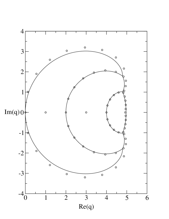
Figure 2: Singular locus ${\cal B}$ in the $q$ plane for the $m\to\infty$ limit of the Potts model partition function $Z(G[(K_{3})_{m},jn],q,v)$ for $v=-0.9$. For comparison, zeros of this partition function are shown for $m=20$ (i.e., $|V|=60$).

3 Flow Polynomials for $G[(K_{r})_{m},jn]$

We first note the

Corollary 3

$$F(G[(K_{r})_{m},jn],q)=(-1)^{3mr(r-1)/2}\sum_{d=0}^{r}\mu_{d}\sum_{j=1}^{n_{T}(r,d)}(\lambda_{T,r,d,j}(x=0,y=1-q))^{m}\ .$$ (3.1)

Proof  This follows immediately from combining eqs. (1.4.11) and (2.1) and using (1.2.1). $\Box$

It will be convenient to write (3.1) simply as

$$F(G[(K_{r})_{m},jn],q)=\sum_{d=0}^{r}\mu_{d}\sum_{j=1}^{n_{T}(r,d)}(\lambda_{F,r,d,j})^{m}$$ (3.2)

where

$$\lambda_{F,r,d,j}=(-1)^{3r(r-1)/2}\lambda_{T,r,d,j}\ .$$ (3.3)

Since $G[(K_{1})_{m},jn]=C_{m}$, it follows that $F(G[(K_{1})_{m},jn],q)=F(C_{m},q)$. This is elementary:

$$F(C_{m},q)=q-1\ .$$ (3.4)

The flow polynomial for $G[(K_{2})_{m},jn]$ can be obtained from our previous calculation of the Tutte polynomial for this family [22]:

$$F(G[(K_{2})_{m},jn],q)=\sum_{d=0}^{2}\mu_{d}\sum_{j=1}^{n_{T}(2,d)}(\lambda_{F,2,d,j})^{m}$$ (3.5)

where $n_{T}(2,0)=2$, $n_{T}(2,1)=2$, $n_{T}(2,2)=1$, and

$$\lambda_{F,2,0,j}=\frac{1}{2}\left[(q-2)(q^{2}-3q+4)\pm\sqrt{R_{F20}}\ \right]\quad{\rm for}\ \ j=1,2$$ (3.6)

with

$$R_{F20}=(q-2)(q-3)(q^{4}-5q^{3}+14q^{2}-20q+12)$$ (3.7)

$$\lambda_{F,2,1,j}=\frac{1}{2}\left[q^{3}-5q^{2}+10q-10\pm\sqrt{R_{F21}}\ \right]\quad{\rm for}\ \ j=1,2$$ (3.8)

where

$$R_{F21}=q^{6}-10q^{5}+45q^{4}-120q^{3}+208q^{2}-224q+116\ .$$ (3.9)

and

$$\lambda_{F,2,2,1}\equiv\lambda_{F,2,2}=-2$$ (3.10)

The flow polynomials for the first few values of $m$ are

$$F(G[(K_{2})_{1},jn],q)=(q-1)^{3}(q-2)$$ (3.11)

$$F(G[(K_{2})_{2},jn],q)=(q-1)(q-2)^{2}(q^{4}-5q^{3}+12q^{2}-16q+10)$$ (3.12)

$$F(G[(K_{2})_{3},jn],q)=(q-1)(q-2)^{2}(q^{2}-4q+5)(q^{5}-6q^{4}+18q^{3}-34q^{2}+37q-28)$$ (3.13)

It is elementary to show that in general, $F(G[(K_{2})_{m},jn],q)$ has the factor $(q-1)(q-2)$.

In Fig. 3 we show the continuous accumulation set ${\cal B}$ of the zeros of $F(G[(K_{2})_{m},jn],q)$ as $m\to\infty$. Some curves on ${\cal B}$ extend to complex infinity, so that ${\cal B}$ is noncompact, in the $q$ plane. Hence, it is also convenient to display ${\cal B}$ in the plane of the variable

$$u=\frac{1}{q}\ .$$ (3.14)

The locus ${\cal B}$ separates the $q$ plane (or equivalently, the $1/q$ plane) into several regions, including four regions that contain intervals of the real axis, together with two pairs of complex-conjugate regions. Six curves forming three complex-conjugate pairs lying on the locus ${\cal B}$ extend infinitely far from the origin of the $q$ plane. In the $u$ plane, these curves (taken in their totality) have a multiple intersection point, in the sense of algebraic geometry, at the origin. We introduce polar coordinates, letting

$$u=|u|e^{i\theta_{u}}\ .$$ (3.15)

We have

Corollary 4

$$\theta_{u}=\frac{(2j+1)\pi}{6}\quad{\rm for}\ \ 0\leq j\leq 5$$ (3.16)

i.e., $\theta_{u}=\pm\pi/6$, $\pm\pi/2$, and $\pm 5\pi/6$.

Proof  To prove this, we note first that the two terms that are dominant in the vicinity of $u=0$ are $\lambda_{F,2,0,1}$ and $\lambda_{F,2,1,1}$. We extract a factor of $q^{3}$ from these, defining $\bar{\lambda}_{F,2,d,j}=q^{-3}\lambda_{F,2,d,j}$, express the $\bar{\lambda}_{F,2,d,j}$ in terms of $u$, and carry out a Taylor series expansion of these in the vicinity of $u=0$, to find

$$\bar{\lambda}_{F,2,0,1}=1-5u+10u^{2}-9u^{3}+O(u^{4})\quad{\rm as}\ \ u\to 0$$ (3.17)

$$\bar{\lambda}_{F,2,1,1}=1-5u+10u^{2}-10u^{3}+O(u^{4})\quad{\rm as}\ \ u\to 0$$ (3.18)

The equation of the degeneracy of magnitudes of leading terms in the vicinity of $u=0$, $|\lambda_{F,2,0,1}|=|\lambda_{F,2,1,1}|$, yields the condition

$$|u|^{3}\cos 3\theta_{u}=0\quad{\rm for}\ \ |u|<<1$$ (3.19)

implying that $\cos 3\theta_{u}=0$, which yields the result (3.16). $\Box$.

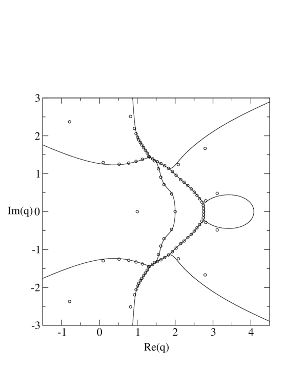
Figure 3: Singular locus ${\cal B}$ in the $q$ plane for the $m\to\infty$ limit of the flow polynomial $F(G[(K_{2})_{m},jn],q)$. For comparison, zeros of the flow polynomial $F(G[(K_{2})_{m},jn],q)$ are shown for $m=30$ (i.e., $|V|=60$).

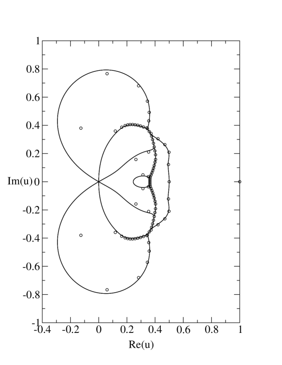
Figure 4: Singular locus ${\cal B}$ in the $u=1/q$ plane for the $m\to\infty$ limit of the flow polynomial $F(G[(K_{2})_{m},jn],q)$. For comparison, zeros of the flow polynomial $F(G[(K_{2})_{m},jn],q)$ are shown for $m=30$ (i.e., $|V|=60$).

The locus ${\cal B}$ crosses the real axis at three points. The largest of these we denote $q_{c}$; this has the value

$$q_{c}(F(G[(K_{2})_{\infty},jn])=4.079828...$$ (3.20)

The other two crossings occur at

$$q_{1}=2.7760454...$$ (3.21)

and

$$q=2\ .$$ (3.22)

The point $q_{c}$ is the larger of the two real solutions of the equation

$$q^{4}-7q^{3}+13q^{2}-q-14=0$$ (3.23)

which is the equation of degeneracy in magnitudes of dominant terms $|\lambda_{F,2,0,1}|=|\lambda_{F,2,1,1}|$. The point $q_{1}$ is the real solution of the equation of degeneracy in magnitudes of dominant terms $|\lambda_{F,2,1,1}|=|\lambda_{F,2,2}|$,

$$q^{3}-4q^{2}+7q-10=0\ .$$ (3.24)

The four regions that contain intervals of the real axis, together with the respective intervals, are: (i) $R_{1}$, $q\geq q_{c}$, (ii) $R_{2}$, $q_{1}\leq q\leq q_{c}$, (iii) $R_{3}$, $2\leq q\leq q_{1}$, and (iv) $R_{4}$, $q\leq 2$. The two complex-conjugate regions are denoted $R_{5},R_{5}^{*}$ and $R_{6},R_{6}^{*}$; in Fig. 3, as one moves counterclockwise from $R_{1}$ into the upper half $q$-plane, one traverses $R_{5}$, containing the point $q=2+2i$, and then $R_{6}$, containing $q=2i$. As is evident in Fig. 3, the density of zeros is rather different along different portions of ${\cal B}$.

In region $R_{1}$, with an appropriate choice of branch cuts, the dominant $\lambda$ is $\lambda_{F,2,0,1}$ so that

$$\phi(G[(K_{2})_{\infty},jn],q)=(\lambda_{F,2,0,1})^{1/2}\quad{\rm for}\ \ q\in R_{1}\ .$$ (3.25)

In region $R_{2}$, the dominant $\lambda$ is $\lambda_{F,2,1,1}$ so that

$$|\phi(G[(K_{2})_{\infty},jn],q)|=|\lambda_{F,2,1,1}|^{1/2}\quad{\rm for}\ \ q\in R_{2}\ .$$ (3.26)

(Recall that in regions other than $R_{1}$, only $|\phi|$ can be obtained unambiguously.) In region $R_{3}$, $\lambda_{F,2,2}$ is dominant and

$$|\phi(G[(K_{2})_{\infty},jn],q)|=\sqrt{2}\quad{\rm for}\ \ q\in R_{3}\ .$$ (3.27)

In region $R_{4}$, with an appropriate choice of square root branch cut, $\lambda_{F,2,1,2}$ is dominant and

$$|\phi(G[(K_{2})_{\infty},jn],q)|=|\lambda_{F,2,1,2}|^{1/2}\quad{\rm for}\ \ q\in R_{4}\ .$$ (3.28)

In $R_{5}$ and $R_{6}$, $\lambda_{F,2,1,2}$ and $\lambda_{F,2,0,1}$ dominate, respectively. We also note that there are several $T$ intersection points on ${\cal B}$.

From our calculation of $T(G[(K_{3})_{m},jn],x,y)$ presented here, one can obtain the corresponding flow polynomial $F(G[(K_{3})_{m},jn],q)$. Since the expressions are rather lengthy, we omit the details.

4 Reliability Polynomials for $G[(K_{r})_{m},jn]$

We proceed to discuss reliability polynomials for $G[(K_{r})_{m},jn]$. Since $G[(K_{1})_{m},jn]$ is the circuit graph $C_{m}$, the result is elementary:

$$R(C_{m},p)=p^{m-1}[m(1-p)+p]\ .$$ (4.1)

Note that when one sets $x=1$, the two $\lambda_{T,r=1,d,j}$ simplify: $\lambda_{T,1,0,1}=x$ becomes equal to $\lambda_{T,1,1,1}=1$, so that Hence, the total number of distinct terms $N_{T,r=1,\lambda}=2$ in the Tutte polynomial is reduced to $N_{R,r=1,\lambda}=1$ for the reliability polynomial. This reduction generalizes to higher $r$. The reliability polynomial $R(C_{m},p)$ evidently has $m-1$ zeros at $p=0$ and one other zero, at $p=m/(m-1)$. As $m\to\infty$, this other zero approaches 1 from above.

The reliability polynomial for $G[(K_{2})_{m},jn]$ can be obtained from our previous calculation of the Tutte polynomial for this family of graphs [22]. Setting $x=1$, we find that two of the five $\lambda$’s in the full Tutte polynomial become equal to two others:

$$\lambda_{T,2,0,1}=\lambda_{T,2,1,1}=\frac{1}{2}\left[(y+2)(y^{2}+3)+\sqrt{R_{2}}\ \right]$$ (4.2)

$$\lambda_{T,2,0,2}=\lambda_{T,2,1,2}=\frac{1}{2}\left[(y+2)(y^{2}+3)-\sqrt{R_{2}}\ \right]$$ (4.3)

where

$$R_{2}=36+44y+33y^{2}+16y^{3}+10y^{4}+4y^{5}+y^{6}\ .$$ (4.4)

Hence, $N_{T,2,\lambda}=5$ is reduced to $N_{R,2,\lambda}=3$ for the reliability polynomial. Setting $y=1/(1-p)$ and inserting the appropriate prefactors according to (1.4.12), we obtain

$$R(G[(K_{2})_{m},jn],p)=p^{2m}\biggl{[}(\alpha_{2,1})^{m}+(\alpha_{2,2})^{m}-\frac{3}{2}(\alpha_{2,3})^{m}+$$ (4.5)

(4.6)

$$mp^{-1}(1-p)^{4}\biggl{\{}(\alpha_{2,1})^{m-1}D_{2,1}+(\alpha_{2,2})^{m-1}D_{2,2}\biggr{\}}\biggr{]}$$ (4.7)

where

$$\alpha_{2,j}=\frac{1}{2}\Bigl{[}(3-2p)(4-6p+3p^{2})\pm\sqrt{R_{2p}}\ \Bigr{]}\quad{\rm for}\ \ j=1,2$$ (4.8)

$$R_{2p}=36p^{6}-260p^{5}+793p^{4}-1308p^{3}+1236p^{2}-640p+144$$ (4.9)

$$D_{2,j}=\frac{1}{2}\left[3\pm\frac{(36-88p+69p^{2}-18p^{3})}{\sqrt{R_{2p}}}\ \right]\quad{\rm for}\ \ j=1,2$$ (4.10)

$$\alpha_{2,3}=2(1-p)^{3}\ .$$ (4.11)

As examples, skipping the degenerate case $m=1$, the reliability polynomials for $G[(K_{2})_{2},jn]$ for the lowest two cases $m=2,3$ are

$$R(G[(K_{2})_{2},jn],p)=p^{3}(2-p)(6p^{6}-44p^{5}+139p^{4}-242p^{3}+246p^{2}-140p+36)$$ (4.12)

and

$$R(G[(K_{2})_{3},jn],p)=p^{5}(120p^{10}-1440p^{9}+7830p^{8}-25440p^{7}+54780p^{6}-81840p^{5}$$ (4.13)

(4.14)

$$+86110p^{4}-63195p^{3}+31080p^{2}-9300p+1296)$$ (4.15)

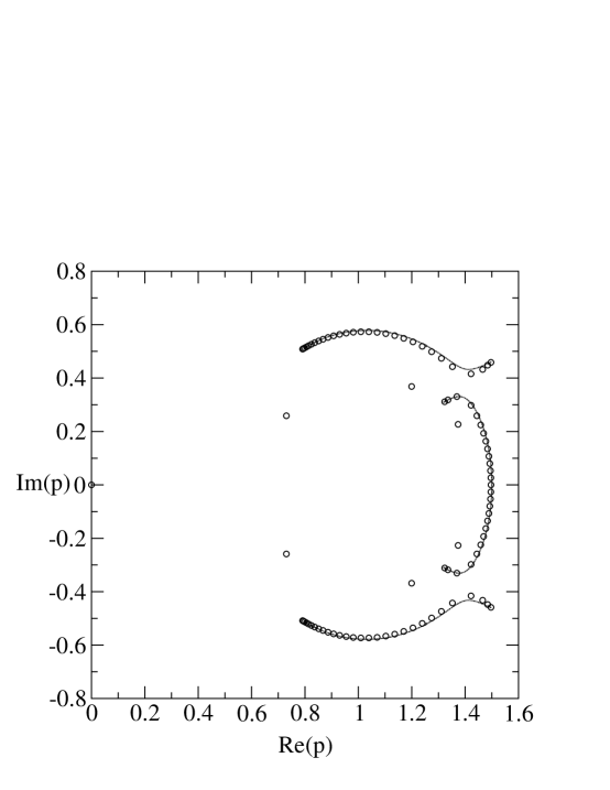
Figure 5: Singular locus ${\cal B}$ in the complex $p$ plane for the $m\to\infty$ limit of the reliability polynomial $R(G[(K_{2})_{m},jn],p)$. For comparison, zeros of the reliability polynomial $R(G[(K_{2})_{m},jn],p)$ are shown for $m=30$ (i.e., $|V|=60$).

In Fig. 5 we show the continuous accumulation set ${\cal B}$ of the zeros of $R(G[(K_{2})_{m},jn],p)$ in the limit $m\to\infty$. This locus is comprised of a self-conjugate arc that crosses the real axis at $p=3/2$ and terminates at approximately $p=1.320\pm 0.309i$, together with a complex-conjugate pair of arcs. The upper arc extends between endpoints at $0.790+0.508i$ and $1.501+0.462i$. The six endpoints of the arcs occur at the zeros of $R_{2p}$, where there are square root branch point singularities in some of the $\lambda$’s. This locus ${\cal B}$ does not separate the $p$ plane into different regions. In passing, we observe that our results are in accord with the conjecture [91] that for an arbitrary (connected) graph $G$, the roots of $R(G,p)$ lie in the disk $|p-1|\leq 1$.

5 Acyclic Orientations for Recursive Families of Graphs

5.1 General

We recall from the introduction the definition of acyclic orientations and the relations (1.5.2) and (1.5.3) expressing the number of acyclic orientations $a(G)$ in terms of a valuation of the chromatic or Tutte polynomial. First we note that for the recursive families of graphs of interest here, namely cyclic or cylindrical strips of regular lattices, $a(G_{m})$ grows exponentially as $m\to\infty$. This follows from the relation (1.5.2) and the structural result (1.6.6). This motivates the definition

Def.  Consider a recursive family of graphs $G_{m}$ and the limit $m\to\infty$. Then we define

$$\alpha(\{G\})=\lim_{|V|\to\infty}a(G)^{1/|V|}\ .$$ (5.1.1)

The number of acyclic orientations can also be generalized [96] to $a_{s}(G)$, given by

$$a_{s}(G)=(-1)^{|V|}P(G,q=-s)\quad{\rm for}\ \ s\in{\mathbb{Z}}_{+}\ .$$ (5.1.2)

with $a_{1}(G)\equiv a(G)$.

Def. Let $G_{m}$ be a recursive family of graphs, such as strips of regular lattices of length $m$, and consider the limit $m\to\infty$. Then

$$\alpha_{s}(\{G\})=\lim_{|V|\to\infty}(a_{s}(G))^{1/|V|}\ .$$ (5.1.3)

Hence,

$$\alpha_{s}(\{G\})=W(\{G\},q=-s)\ .$$ (5.1.4)

and, in particular, $\alpha(\{G\})=W(\{G\},q=-1)$.

In our previous studies of chromatic polynomials and the resultant singular loci ${\cal B}$ for a variety of recursive families of graphs including strips of regular lattices, we found that ${\cal B}$ never intersects the negative real $q$ axis, and, indeed, the points $q=-s$ for $s\in{\mathbb{Z}}_{+}$ are in region $R_{1}$. Hence, for the recursive families of interest here, there is no ambiguity in which $1/|V|$’th root to choose in evaluating (1.4.5) at the points $q=-s$, $s\in{\mathbb{Z}}_{+}$. (For families with noncompact ${\cal B}$, as is evident from the plots of respective loci ${\cal B}$ presented in [53, 62, 63, 64], although ${\cal B}$ does not intersect the negative real axis, it can separate the point $q=-s$ from the region $R_{1}$; we do not consider such families here.) Because the points $q<0$ are in region $R_{1}$ for the strip graphs of regular lattices, we can apply a previous result [15] to infer that $\alpha_{s}(\{G\})$ is independent of the longitudinal boundary conditions. Thus, for example, $\alpha_{s}(\{G\})$ is the same for the $m\to\infty$ limit of the square-lattice strip graphs $sq(L_{y},L_{x},FBC_{y},FBC_{x})$, $sq(L_{y},L_{x},FBC_{y},PBC_{x})$, and $sq(L_{y},L_{x},FBC_{y},TPBC_{x})$, and therefore we shall omit the longitudinal boundary condition in listing the values that we obtain in these cases. Henceforth, we shall focus on the $s=1$ case, i.e., acyclic orientations.

5.2 $a(G)$ and $\alpha(\{G\})$ for Strips of the Square Lattice

We first list some elementary results. For a tree graph,

$$a(T_{n})=2^{n-1}\ .$$ (5.2.1)

For a circuit graph,

$$a(C_{n})=2^{n}-2$$ (5.2.2)

whence

$$\alpha(\{T\})=\alpha(\{C\})=\alpha(sq,L_{y}=1)=2\ .$$ (5.2.3)

Another easy result is

$$a(sq,L_{y}=2,L_{x}=m,FBC_{y},FBC_{x})=2\cdot 7^{m}$$ (5.2.4)

From $P(sq[L_{y}=2,L_{x}=m,FBC_{y},(T)PBC_{x}],q)$ calculated in [7], we find

$$a(sq,L_{y}=2,L_{x}=m,FBC_{y},PBC_{x})=7^{m}-2\cdot 4^{m}-2^{m+1}+5$$ (5.2.5)

$$a(sq,L_{y}=2,L_{x}=m,FBC_{y},TPBC_{x})=7^{m}-2\cdot 4^{m}+2^{m+1}-1$$ (5.2.6)

From any of (5.2.4), (5.2.5), or (5.2.6), it follows that

$$\alpha(sq,L_{y}=2,FBC_{y})=\sqrt{7}=2.645751...$$ (5.2.7)

From $P(sq[L_{y}=3,L_{x}=m,FBC_{y},PBC_{x}],q)$ calculated in [68, 69], we find

$$a(sq,L_{y}=3,L_{x}=m,FBC_{y},PBC_{x}) = -13+5(2^{m}+3^{m}+5^{m})-2\cdot 9^{m}-2S_{m}$$ (5.2.10)

$$+\Biggl{(}\frac{27+\sqrt{481}}{2}\Biggr{)}^{m}+\Biggl{(}\frac{27-\sqrt{481}}{2}\Biggr{)}^{m}$$

and from $P(sq[L_{y}=3,L_{x}=m,FBC_{y},TPBC_{x}],q)$ calculated in [70], we find

$$a(sq,L_{y}=3,L_{x}=m,FBC_{y},TPBC_{x}) = 5-2^{m}+3^{m}-5^{m}+2\cdot 9^{m}-2S_{m}$$ (5.2.13)

$$+\Biggl{(}\frac{27+\sqrt{481}}{2}\Biggr{)}^{m}+\Biggl{(}\frac{27-\sqrt{481}}{2}\Biggr{)}^{m}$$

with

$$S_{m}=\sum_{j=1}^{3}(-\lambda_{sqpxy3,j})^{m}$$ (5.2.14)

where the $\lambda_{sqpxy3,j}$, $j=1,2,3$, are the roots of the equation

$$\xi^{3}+23\xi^{2}+134\xi+202=0$$ (5.2.15)

From either of (5.2.10) or (5.2.13) we have

$$\alpha(sq,L_{y}=3,FBC_{y})=\Biggl{(}\frac{27+\sqrt{481}\ }{2}\Biggr{)}^{1/3}=2.903043...$$ (5.2.16)

From the chromatic polynomial $P(sq[L_{y}=4,L_{x},FBC_{y},FBC_{x}],q)$ calculated in [59], we obtain

$$\alpha(sq,L_{y}=4,FBC_{y})=(\lambda_{sqxy4,max})^{1/4}=3.040731...$$ (5.2.17)

where $\lambda_{sqxy4,max}$ is the largest root of the cubic equation

$$\xi^{3}-105\xi^{2}+1747\xi-6758=0\ .$$ (5.2.18)

From chromatic polynomials calculated in [76] and [23], we obtain the values of $\alpha(sq,L_{y},FBC_{y})$ for $L_{y}$ up to 8. The results are listed in Table 2.

We next consider strips of the square lattice with cylindrical boundary conditions. An elementary calculation yields

$$a(sq,L_{y}=3,L_{x}=m,PBC_{y},FBC_{x})=6\cdot(34)^{m}$$ (5.2.19)

whence

$$\alpha(sq,L_{y}=3,PBC_{y})=(34)^{1/3}=3.2396118...$$ (5.2.20)

From the chromatic polynomial $P(sq[L_{y}=4,L_{x},PBC_{y},FBC_{x}],q)$ calculated in [61] we obtain

$$\alpha(sq,L_{y}=4,PBC_{y})=\Biggl{(}\frac{139+\sqrt{16009}\ }{2}\Biggr{)}^{1/4}=3.3944509...$$ (5.2.21)

From the chromatic polynomials $P(sq[L_{y},L_{x},PBC_{y},FBC_{x}],q)$ for $L_{y}=5,6$ calculated in [61] we compute

$$\alpha(sq,L_{y}=5,PBC_{y})=\Biggl{(}\frac{527+\sqrt{200585}\ }{2}\Biggr{)}^{1/5}=3.4481257...$$ (5.2.22)

and

$$\alpha(sq,L_{y}=6,PBC_{y})=(\lambda_{sqpxpy6,max})^{1/6}=3.4705457...$$ (5.2.23)

where $\lambda_{sqpxpy6,max}$ is the largest root of the equation

$$\xi^{5}-2049\xi^{4}+547805\xi^{3}-36633324\xi^{2}+639262524\xi-2756653440=0\ .$$ (5.2.24)

We have also computed $\alpha(sq,L_{y},PBC_{y})$ for $L_{y}$ up to 12 using chromatic polynomials calculated in [82]. The results are listed in Table 2.

Table 2: Values of $\alpha(\{G\})$ for the infinite-length limits of strip graphs of the square lattice with width $L_{y}$ vertices and free (F) or periodic (P) transverse boundary conditions.

$L_{y}$	$BC_{y}$	$\alpha(\{G\})$
1	F	2
2	F	2.646
3	F	2.903
4	F	3.041
5	F	3.126
6	F	3.185
7	F	3.227
8	F	3.259
3	P	3.240
4	P	3.394
5	P	3.448
6	P	3.471
7	P	3.481
8	P	3.487
9	P	3.490
10	P	3.491
11	P	3.492
12	P	3.493

A basic property of $\alpha(sq,L_{y},BC_{y})$, where $BC_{y}$ denotes the transverse boundary condition, (free, $FBC_{y}$ or periodic, $PBC_{y}$) is that, owing to the fact that one can calculate this quantity (and indeed, more generally, the chromatic or Tutte polynomial from which it is derived by a special valuation) by transfer matrix methods, it follows that $\alpha(sq,L_{y},BC_{y})$ is a monotonically increasing function of $L_{y}$ [98, 99]. A similar monotonicity holds for $\alpha(tri,L_{y},BC_{y})$ for strips of the triangular lattice (see further below). We also observe that for a given strip width $L_{y}$, the value of $\alpha$ for periodic transverse boundary conditions is greater than the value for free transverse boundary conditions. This is easily understood since the transverse boundary effects are reduced when one uses periodic transverse boundary conditions, and hence the resultant $\alpha$ should be closer to that for the infinite square lattice. Let us denote $\alpha_{sq}\equiv\lim_{L_{y}\to\infty}\alpha(sq,L_{y},BC_{y})$. Given the monotonically increasing property of $\alpha(sq,L_{y},BC_{y})$ as a function of $L_{y}$, our results show that $\alpha_{sq}>3.49287$ (rounded off to 3.493 in the table) for this lattice. This value is a slight improvement of the recent lower bounds $\alpha_{sq}\geq 22/7=3.1428...$ [98] and $\alpha_{sq}\geq 3.41358$ [99]. Since the upper bounds $\alpha_{sq}\leq 3.70925$ [98] and $\alpha_{sq}\leq 3.55449$ [99] have also been established, the value of $\alpha_{sq}$ has now been rather well restricted.

5.3 $a$ and $\alpha$ for Strips of the Triangular Lattice

For a strip of the triangular lattice, formed by starting with a square strip and adding diagonal edges, say from the upper left to the lower right vertices of each square, with free longitudinal boundary conditions, an elementary calculation yields

$$a(tri,L_{y}=2,L_{x}=m,FBC_{y},FBC_{x})=2\cdot 3^{2m}\ .$$ (5.3.1)

For cyclic and Möbius strips of the triangular lattice with width $L_{y}=2$, from the chromatic polynomials in [68], we find

$$a(tri,L_{y}=2,L_{x}=m,FBC_{y},PBC_{x})=3^{2m}-2\Biggl{[}\biggl{(}\frac{7+\sqrt{13}\ }{2}\biggr{)}^{m}+\biggl{(}\frac{7-\sqrt{13}\ }{2}\biggr{)}^{m}\Biggr{]}+5$$ (5.3.2)

$$a(tri,L_{y}=2,L_{x}=m,FBC_{y},TPBC_{x})=3^{2m}+\frac{8}{\sqrt{13}}\Biggl{[}-\biggl{(}\frac{7+\sqrt{13}\ }{2}\biggr{)}^{m}+\biggl{(}\frac{7-\sqrt{13}\ }{2}\biggr{)}^{m}\Biggr{]}-1$$ (5.3.3)

Using any of (5.3.1), (5.3.2), or (5.3.3), we compute

$$\alpha(tri,L_{y}=2,FBC_{y})=3$$ (5.3.4)

For $L_{y}=3$, using [78], we get

$$a(tri,L_{y}=3,L_{x}=m,FBC_{y},PBC_{x}) = -13+5\Biggl{[}3^{m}+\Biggl{(}\frac{9+\sqrt{33}\ }{2}\Biggr{)}^{m}+\Biggl{(}\frac{9-\sqrt{33}\ }{2}\Biggr{)}^{m}\Biggr{]}$$ (5.3.7)

$$-2(12^{m}+R_{m})+\Biggl{(}\frac{43+\sqrt{1417}\ }{2}\Biggr{)}^{m}+\Biggl{(}\frac{43-\sqrt{1417}\ }{2}\Biggr{)}^{m}$$

with

$$R_{m}=\sum_{j=1}^{3}(-\lambda_{t3c,j})^{m}$$ (5.3.10)

where the $\lambda_{t3c,j}$, $j=1,2,3$, are the roots of the equation

$$\xi^{3}+33\xi^{2}+201\xi+324=0$$ (5.3.11)

whence

$$\alpha(tri,L_{y}=3,FBC_{y})=\biggl{(}\frac{43+\sqrt{1417}\ }{2}\biggr{)}^{1/3}=3.4290909...$$ (5.3.12)

and, for $L_{y}=4,5$,

$$\alpha(tri,L_{y}=4,FBC_{y})=(\lambda_{trixy4,max})^{1/4}=3.665350...$$ (5.3.13)

where $\lambda_{trixy4,max}$ is the largest root of the quartic equation

$$\xi^{4}-217\xi^{3}+6960\xi^{2}-67968\xi+186624=0$$ (5.3.14)

$$\alpha(tri,L_{y}=5,FBC_{y})=(-\lambda_{trixy5,max})^{1/5}=3.81486986...$$ (5.3.15)

where $\lambda_{txy5,max}$ is the root with the largest magnitude of the equation

$$\xi^{9}+1160\xi^{8}+330071\xi^{7}+39854484\xi^{6}+2509883184\xi^{5}+87798785472\xi^{4}+1684802267136\xi^{3}$$ (5.3.16)

(5.3.17)

$$+16500631191552\xi^{2}+73085995450368\xi+104764180267008=0$$ (5.3.18)

(5.3.19)

(5.3.20)

For strips of the triangular lattice with cylindrical boundary conditions, one has

$$a(tri,L_{y}=3,L_{x}=m,PBC_{y},FBC_{x})=6\cdot(71)^{m}$$ (5.3.21)

$$\alpha(tri,L_{y}=3,PBC_{y})=(71)^{1/3}=4.1408177...$$ (5.3.22)

For $L_{y}=4$ from the chromatic polynomial calculated in [61] we get

$$\alpha(tri,L_{y}=4,PBC_{y})=(352)^{1/4}=4.3314735...$$ (5.3.23)

Further, using the chromatic polynomials calculated in [78], we have

$$\alpha(tri,L_{y}=5,PBC_{y})=(897+339\sqrt{5}\ )^{1/5}=4.403125...$$ (5.3.24)

$$\alpha(tri,L_{y}=6,PBC_{y})=(\lambda_{txpy6,max})^{1/6}=4.435287...$$ (5.3.25)

where $\lambda_{txpy6,max}$ is the largest root of the equation

$$\xi^{5}-8789\xi^{4}+9102104\xi^{3}-1119801408\xi^{2}+42084913152\xi-364032294912=0\ .$$ (5.3.26)

The monotonicity of $\alpha(tri,L_{y},FBC_{y})$ and $\alpha(tri,L_{y},PBC_{y})$ as a function of $L_{y}$ is evident in the table. One can, of course, calculate these quantities for larger values of $L_{y}$; however, it is interesting to observe that our exact calculation of $\alpha(tri,L_{y}=6,PBC_{y})$ is already within about 1 % of the exact value for the $L_{y}\to\infty$ limit, i.e., for the infinite triangular lattice, which we have obtained via an evaluation of the $W$ function in [43]:

$$\alpha(tri)=4.474647...$$ (5.3.27)

This shows that the values of $\alpha(tri,L_{y},PBC_{y})$ converge rather rapidly to the infinite-$L_{y}$ value as $L_{y}$ increases.

Table 3: Values of $\alpha(\{G\})$ for the infinite-length limits of strip graphs of the triangular lattice with width $L_{y}$ vertices and free (F) or periodic (P) transverse boundary conditions.

$L_{y}$	$BC_{y}$	$\alpha(\{G\}$
2	F	3
3	F	3.429
4	F	3.665
5	F	3.815
3	P	4.141
4	P	4.331
5	P	4.403
6	P	4.435
$\infty$	P	4.475

5.4 $a$ and $\alpha$ for Cyclic Clan Graphs

From eqs. (1.8.1) and (1.8.2) we have

$$a(G[(K_{r})_{m},jn]) = (-1)^{rm}P(G[(K_{r})_{m},jn],q=-1)$$ (5.4.1)

$$= (-1)^{rm}\left[[(-1-r)_{(r)}]^{m}+2\sum_{d=1}^{r}(-1)^{d}(\lambda_{P,r,d}(q=-1))^{m}\right]$$ (5.4.3)

$$= [(2r)_{(r)}]^{m}+2\sum_{d=1}^{r}(-1)^{d}[r_{(d)}(2r)_{(r-d)}]^{m}$$ (5.4.5)

where we have used

$$\lambda_{P,r,d}(q=-1)=(-1)^{r}r_{(d)}(2r)_{(r-d)}$$ (5.4.6)

and

$$\mu_{d}(q=-1)=(-1)^{d}2\quad{\rm for}\ d\geq 1$$ (5.4.7)

(the $d=0$ coefficient being a constant, $\mu_{0}=1$).

Since the point $q=-1$ is in region $R_{1}$, the term $\lambda_{P,r,d}$ with $d=0$ is dominant, and hence

$$\alpha(G[\{(K_{r})\},jn]=[(2r)_{(r)}]^{1/r}\ .$$ (5.4.8)

For large $r\to\infty$, this has the leading asymptotic behavior $\alpha(G[\{(K_{r})\},jn])\sim 4e^{-1}r$.

6 Number of Spanning Trees for Two $G[(K_{r})_{m},L]$ Families

6.1 General

In this section we shall again consider only connected graphs $G=(V,E)$ and for notational simplicity, we let

$$n=|V|\ .$$ (6.1.1)

We denote the number of spanning trees of such a graph as $N_{ST}(G)$. Here we shall prove theorems that determine the the numbers of spanning trees of two $G[(K_{r})_{m},L]$ families of graphs, namely the cyclic clan graph family $G[(K_{r})_{m},L=jn]$ and the family $G[(K_{r})_{m},L=id]$. In general $N_{ST}(G)$ is given by (1.5.1); however, we shall actually use an alternative method of calculation based on the Laplacian matrix (e.g., [12]). We recall that the adjacency matrix ${\bf A}(G)$ of a graph $G$ is the $n\times n$ matrix whose $jk$’th element is the number of edges connecting vertex $j$ with vertex $k$ in $V$. Next, we recall

Def.  The Laplacian matrix ${\bf Q}(G)$ of this graph is given by

$${\bf Q}(G)={\bf\Delta}(G)-{\bf A}(G)$$ (6.1.2)

where ${\bf\Delta}$ is the $n\times n$ diagonal matrix whose $j$’th diagonal entry is equal to the degree of the $j$’th vertex, $\Delta_{jj}=\Delta(v_{j})$ and whose other entries are zero.

Since the sum of the elements in each row (or column) of ${\bf Q}(G)$ vanishes, one of the eigenvalues of ${\bf Q}(G)$ is zero. Denote the remaining $n-1$ eigenvalues by $\lambda_{1},...,\lambda_{n-1}$. Then a basic theorem is (e.g., [12, 100])

$$N_{ST}(G) = {\rm any\ cofactor\ of\ }{\bf Q}(G)$$ (6.1.3)

$$= \frac{1}{n}\prod_{j=1}^{n-1}\lambda_{j}\ .$$ (6.1.4)

For the recursive families $G_{m}$ of graphs considered here, $N_{ST}(G)$ grows exponentially for large $m$, and hence a quantity of interest is the growth rate. In previous works calculating $z(\{G\})$ and $N_{ST}(G)$ for the $n\to\infty$ limits of regular lattice graphs [101]-[103] the convention was used of defining this growth rate in terms of $\ln N_{ST}^{1/n}$, and we shall follow this convention here:

Def.  Let $G$ be a connected graph. Then the quantity $z(\{G\})$ is defined by

$$\exp(z(\{G\}))=\lim_{n\to\infty}[N_{ST}(G)]^{1/n}\ .$$ (6.1.5)

Since we shall compare the expressions that we derive for $N_{ST}$ on $G[(K_{r})_{m},jn]$ and $G[(K_{r})_{m},id]$ with upper bounds, we recall the statements of these bounds. A general upper bound is [104]

$$N_{ST}(G)\leq\frac{1}{n}\biggl{(}\frac{2|E|}{n-1}\biggr{)}^{n-1}\ .$$ (6.1.6)

For a $\Delta$-regular graph $G$, using the relation $\Delta=2|E|/n$, this implies the upper bound

$$N_{ST}(G)\leq\frac{1}{n}\biggl{(}\frac{n\Delta}{n-1}\biggr{)}^{n-1}$$ (6.1.7)

and hence

$$\exp(z(\{G\}))\leq\Delta\ .$$ (6.1.8)

A stronger upper bound for $\Delta$-regular graphs with vertex degree $\Delta\geq 3$ is [105, 106]:

$$N_{ST}(G)\leq\Biggl{(}\frac{2\ln n}{n\Delta\ln\Delta}\Bigg{)}(C_{\Delta})^{n},$$ (6.1.9)

where

$$C_{\Delta}=\frac{(\Delta-1)^{\Delta-1}}{[\Delta(\Delta-2)]^{\Delta/2-1}}\ .$$ (6.1.10)

yielding the upper bound for a $\Delta$-regular graph with $\Delta\geq 3$

$$\exp(z(\{G\}))\leq C_{\Delta}\ .$$ (6.1.11)

By expanding $C_{\Delta}$ as $\Delta\to\infty$, one sees that in this limit the upper bound (6.1.11) approaches (6.1.8).

For the comparison of a given growth rate of a $\Delta$-regular graph with the two upper bounds (6.1.8) and (6.1.11), labelled as $u.b.,j$ with $j=1,2$, we define the ratios

$$R_{j}(\{G\})=\frac{\exp(z(\{G\}))}{\exp(z(\{G\})_{u.b.,j})}\ .$$ (6.1.12)

6.2 Number of Spanning Trees in $G[(K_{r})_{m},jn]$

Here we shall calculate the number of spanning trees for the graph $G[(K_{r})_{m},jn]$. Let ${\bf a}(j,j^{\prime})$ be the $r\times r$ adjacency matrix between the vertices of $K_{r_{j}}$ and $K_{r_{j^{\prime}}}$. The non-zero entries in this matrix are

$${\bf a}(j,j)={\bf J}_{r}-{\bf I}_{r}\quad{\rm for}\ 1\leq j\leq m$$ (6.2.1)

and

$${\bf a}(j,j+1)={\bf a}(j+1,j)={\bf J}_{r}\quad{\rm for}\ 1\leq j\leq m$$ (6.2.2)

where ${\bf J}_{r}$ is the $r\times r$ matrix with all elements equal to unity, and ${\bf I}_{r}$ is the $r\times r$ identity matrix. The Laplacian matrix of the graph $G[(K_{r})_{m},jn]$ is then

$${\bf Q}(G[(K_{r})_{m},jn]) = [(3r-1){\bf I}_{r}-{\bf a}(j,j)]\otimes{\bf I}_{m}-{\bf a}(j,j+1)\otimes{\bf R}_{m}-{\bf a}(j+1,j)\otimes{\bf R}^{T}_{m}$$ (6.2.3)

$$= (3r{\bf I}_{r}-{\bf J}_{r})\otimes{\bf I}_{m}-{\bf J}_{r}\otimes{\bf R}_{m}-{\bf J}_{r}\otimes{\bf R}^{T}_{m}$$

where ${\bf R}_{m}$ is the $m\times m$ matrix

$${\bf R}_{m}=\left(\begin{array}[]{ccccc}0&1&0&\cdots&0\\ 0&0&1&\cdots&0\\ \vdots&\vdots&\vdots&\ddots&\vdots\\ 0&0&0&\cdots&1\\ 1&0&0&\cdots&0\end{array}\right)\ .$$ (6.2.4)

Lemma 3  The eigenvalues of ${\bf Q}(G[(K_{r})_{m},jn])$ are

$$\lambda({\bf Q}(G[(K_{r})_{m},jn]))=\cases{3r-(r+re^{i2\pi j/m}+re^{-i2\pi j/m})=2r[1-\cos(2\pi j/m)]\ {\rm for}\ j=0,1,\cdots,m-1\cr\cr 3r\quad\quad{\rm with\ multiplicity}\ (r-1)m.}$$ (6.2.5)

Proof  We first observe that ${\bf R}_{m}$ can be diagonalized by the similarity transformation ${\bf S}_{m}{\bf R}_{m}{\bf S}_{m}^{-1}$ generated by the matrix ${\bf S}_{m}$ with elements

$$({\bf S}_{m})_{jk}=({\bf S}_{m}^{-1})^{*}_{jk}=m^{-1/2}e^{i2\pi jk/m}\quad{\rm for}\ j,k=0,1,\cdots,m-1,$$ (6.2.6)

where ^∗ denotes the complex conjugate, and $i=\sqrt{-1}$. Therefore, ${\bf R}_{m}$ has the eigenvalues

$$\lambda_{j}({\bf R}_{m})=e^{i2\pi j/m}\quad{\rm for}\ j=0,1,\cdots,m-1.$$ (6.2.7)

The result in (6.2.5) then follows. $\Box$

Theorem 5

$$N_{ST}(G[(K_{r})_{m},jn])=3^{(r-1)m}r^{rm-2}m\ .$$ (6.2.8)

Proof  From (6.1.4) we obtain the result

$$N_{ST}(G[(K_{r})_{m},jn]) = \frac{1}{rm}(3r)^{(r-1)m}\prod_{j=1}^{m-1}2r[1-\cos(2\pi j/m)]$$ (6.2.9)

$$= \frac{1}{r^{2}m}[r(3r)^{r-1}]^{m}\prod_{j=1}^{m-1}4\sin^{2}(j\pi/m)$$ (6.2.11)

To evaluate the product, we use the relation

$$2^{m-1}\prod_{j=0}^{m-1}\sin(\epsilon+\frac{j\pi}{m})=\sin(m\epsilon)$$ (6.2.12)

taking the limit $\epsilon\to 0$ and applying L’Hospital’s rule. This yields $N_{ST}(G[(K_{r})_{m},jn])=(r^{2}m)^{-1}[r(3r)^{r-1}]^{m}m^{2}$, which, in turn, gives the result in (6.2.8). $\Box$

Corollary 5  Consider the number of spanning trees on the graph $G[(K_{r})_{m},jn]$ and take the limit $m\to\infty$. The quantity measuring the growth rate in this limit is given by

$$\exp(z(G[(K_{r})_{\infty},jn]))=3^{1-\frac{1}{r}}\ r\ .$$ (6.2.13)

Proof  This follows from (6.2.8) and the definition (6.1.5). $\Box$

For the first nontrivial case, $r=2$, eq. (6.2.13) yields $\exp(z(G[(K_{2})_{\infty},jn]))=2\sqrt{3}\simeq 3.46410$, in agreement with our result in eq. (A.16) of [22].

For large $r$, the ratios $R_{i}$, $i=1,2$ both approach unity:

$$R_{1}(G[(K_{r})_{\infty},jn]) = 1+\biggl{(}\frac{1}{3}-\ln 3\biggr{)}r^{-1}$$ (6.2.16)

$$+\biggl{(}\frac{1}{9}-\frac{1}{3}\ln 3+\frac{1}{2}(\ln 3)^{2}\biggr{)}r^{-2}+O(r^{-3})$$

$$\simeq 1-0.76528\ r^{-1}+0.34838\ r^{-2}+O(r^{-3})$$ (6.2.18)

$$R_{2}(G[(K_{r})_{\infty},jn]) = 1+\biggl{(}\frac{1}{2}-\ln 3\biggr{)}r^{-1}$$ (6.2.21)

$$+\biggl{(}\frac{7}{24}-\frac{1}{2}\ln 3+\frac{1}{2}(\ln 3)^{2}\biggr{)}r^{-2}+O(r^{-3})$$

$$\simeq 1-0.59861\ r^{-1}+0.345835\ r^{-2}+O(r^{-3})$$ (6.2.23)

This tendency of the growth rates to approach the upper bounds as the vertex degree increases was also found in [103] for regular lattices.

In Table 4 we list the growth rate (6.2.13) for $2\leq r\leq 10$ and compare it with the upper bounds (6.1.8) and (6.1.11). (We do not list the lowest case, $r=1$, since $N_{ST}$ grows linearly rather than exponentially in $m$ for this value of $r$.)

Table 4: Values of $\exp(z(G[(K_{r})_{\infty},jn]))$, abbreviated as $e^{z}$, from (6.2.13) for $2\leq r\leq 10$ and comparison with the upper bounds (6.1.8) and (6.1.11) via the ratios $R_{j}$, $j=1,2$ given by (6.1.12).

$r$	$e^{z}$	$R_{1}$	$R_{2}$
2	3.464	0.693	0.786
3	6.240	0.780	0.838
4	9.118	0.829	0.871
5	12.041	0.860	0.894
6	14.988	0.882	0.910
7	17.950	0.897	0.921
8	20.920	0.910	0.931
9	23.897	0.919	0.938
10	26.879	0.927	0.944

6.3 Number of Spanning Trees in $G[(K_{r})_{m},id]$

Here we calculate the number of spanning trees in the family of graphs $G[(K_{r})_{m},id]$. In [73] and [85, 86] studies were carried out of the chromatic polynomials of the family $G[(K_{r})_{m},L]$ for general linkage $L$, and the case of the identity linkage $L=id$ was called the bracelet graph, $G[(K_{r})_{m},id]\equiv B_{m}(r)$. Parenthetically, we note that the chromatic polynomial for $G[(K_{r})_{m},id]$ was computed for $r=2$ in [7], for $r=3$ in [74], for $r=4$ in [79] and subsequently, by different methods, in [85], and for $r=5,6$ in [87]. The graph $G[(K_{r})_{m},id]$ has $|V|=mr$, $|E|=(1/2)mr(r+1)$ and is a $\Delta$-regular graph with uniform vertex degree $\Delta=r+1$. For our calculation, we first note that the definition of ${\bf a}(j,j)$ remains the same, as given in (6.2.1) and

$${\bf a}(j,j+1)={\bf a}(j+1,j)={\bf I}_{r}\quad{\rm for}\ 1\leq j\leq m\ .$$ (6.3.1)

The Laplacian matrix for this the $G[(K_{r})_{m},id]$ graph is

$${\bf Q}(G[(K_{r})_{m},id]) = [(r+1){\bf I}_{r}-{\bf a}(j,j)]\otimes{\bf I}_{m}-{\bf a}(j,j+1)\otimes{\bf R}_{m}-{\bf a}(j+1,j)\otimes{\bf R}^{T}_{m}$$ (6.3.2)

$$[(r+2){\bf I}_{r}-{\bf J}_{r}]\otimes{\bf I}_{m}-{\bf I}_{r}\otimes{\bf R}_{m}-{\bf I}_{r}\otimes{\bf R}^{T}_{m}$$

Lemma 4  The eigenvalues of ${\bf Q}(G[(K_{r})_{m},id])$ are

$$\lambda({\bf Q}(G[(K_{r})_{m},id])=\cases{r+2-(r+e^{2i\pi j/m}+e^{-2i\pi j/m})=2[1-\cos(2\pi j/m)]&for $j=0,1,\cdots,m-1$\cr\cr r+2-(e^{2i\pi j/m}+e^{-2i\pi j/m})=r+2[1-\cos(2\pi j/m)]&with multiplicity $(r-1)$.}$$ (6.3.3)

The proof proceeds in the same way as before, and is omitted.

Theorem 6  The number of spanning trees in $G[(K_{r})_{m},id]$ is

$$N_{ST}(G[(K_{r})_{m},id])=\cases{mr^{r-2}\Biggl{[}(r+4)(\frac{\omega^{m/2}-\omega^{-m/2}}{\omega-\omega^{-1}})^{2}\Biggr{]}^{r-1}&for even $m$\cr\cr mr^{r-2}(\frac{\omega^{m}-2+\omega^{-m}}{\omega-2+\omega^{-1}})^{r-1}&for odd $m$.}$$ (6.3.4)

where

$$\omega=\frac{r+2+\sqrt{r(r+4)}}{2}\ .$$ (6.3.5)

Proof  We first use the lemma (6.3.3) with (6.1.4) to obtain

$$N_{ST}(G[(K_{r})_{m},id]) = \frac{1}{rm}\Biggl{[}\prod_{j=1}^{m-1}2[1-\cos(2\pi j/m)]\Biggr{]}\prod_{k=0}^{m-1}\Biggl{[}r+2[1-\cos(2\pi k/m)]\Biggr{]}^{r-1}$$ (6.3.6)

$$= mr^{r-2}\Biggl{[}\prod_{k=1}^{m-1}[r+2-2\cos(2\pi k/m)]\Biggr{]}^{r-1}\ .$$ (6.3.8)

For even $m$, the product can be evaluated by using the identity

$$\prod_{k=1}^{m-1}[x^{2}-2x\cos(k\pi/m)+1]=\frac{x^{2m}-1}{x^{2}-1}$$ (6.3.9)

and setting $x=\omega$ to get

$$\prod_{k=1}^{m-1}[r+2-2\cos(2\pi k/m)] = (r+4)\Biggl{[}\prod_{k=1}^{m/2-1}[r+2-2\cos(\pi k/(m/2))]\Biggr{]}^{2}$$ (6.3.10)

$$= (r+4)\Biggl{[}\omega^{1-\frac{m}{2}}\biggl{(}\frac{\omega^{m}-1}{\omega^{2}-1}\biggr{)}\Biggr{]}^{2}$$ (6.3.12)

$$= (r+4)\Biggl{[}\frac{\omega^{m/2}-\omega^{-m/2}}{\omega-\omega^{-1}}\Biggr{]}^{2}\ .$$ (6.3.14)

For odd $m$, we use the equation

$$\prod_{k=1}^{m}[\omega^{2}-2\omega\cos(2\pi k/(2m+1))+1]=\frac{\omega^{2m+1}-1}{\omega-1}$$ (6.3.15)

with the same substitution (6.3.5) for $\omega$, to obtain

$$\prod_{k=1}^{m-1}[r+2-2\cos(2\pi k/m)] = \Biggl{[}\prod_{k=1}^{(m-1)/2}[r+2-2\cos(2\pi k/m)]\Biggr{]}^{2}$$ (6.3.16)

$$= \Biggl{[}\omega^{(1-m)/2}\biggl{(}\frac{\omega^{m}-1}{\omega-1}\biggr{)}\Biggr{]}^{2}$$ (6.3.18)

$$= \frac{\omega^{m}-2+\omega^{-m}}{\omega-2+\omega^{-1}}\ .$$ (6.3.20)

Combining eqs. (6.3.8), (6.3.14) and (6.3.20), we then have the result given in (6.3.4). $\Box$

We remark that the generating function of $\frac{\omega^{m/2}-\omega^{-m/2}}{\omega-\omega^{-1}}$ for even $m$ is $1/(1-(r+2)\zeta+\zeta^{2})$, and the generating function of $\frac{\omega^{m/2}-\omega^{-m/2}}{\omega^{1/2}-\omega^{-1/2}}$ for odd $m$ is $(1+\zeta)/(1-(r+2)\zeta+\zeta^{2})$.

Corollary 6  Consider the number of spanning trees on the graph $G[(K_{r})_{m},id]$ and take the limit $m\to\infty$. The quantity measuring the growth rate in this limit is given by $\omega^{1-\frac{1}{r}}$, i.e.,

$$\exp(z(G[(K_{r})_{\infty},id]))=\Biggl{[}\frac{r+2+\sqrt{r(r+4)}}{2}\ \Biggr{]}^{1-\frac{1}{r}}\ .$$ (6.3.21)

Proof  This follows from (6.3.4) and the definition (6.1.5). $\Box$

For $r=1$, $\exp(z(G[(K_{1})_{\infty},id]))=1$, reflecting the fact that $N_{ST}=m$ for $G[(K_{1})_{m},id]=C_{m}$, which is subexponential growth in $m$. For $r=2$,

$$\exp(z(G[(K_{2})_{\infty},id]))=(2+\sqrt{3}\ )^{1/2}\simeq 1.93185$$ (6.3.22)

in agreement with our result in eq. (D.21) of [18]. For $r=3$,

$$\exp(z(G[(K_{3})_{\infty},id]))=\biggl{(}\frac{5+\sqrt{21}}{2}\ \biggr{)}^{2/3}\simeq 2.84207$$ (6.3.23)

in agreement with our result in eq. (A.88) of [19].

For large $r$, the ratios $R_{i}$, $i=1,2$ both approach unity in the manner indicated below:

$$R_{1}(G[(K_{r})_{\infty},id]) = 1+(1-\ln r)r^{-1}$$ (6.3.26)

$$+\Bigl{(}-4-\ln r+\frac{1}{2}\ln^{2}r\Bigr{)}r^{-2}+O\biggl{(}\Bigl{(}\frac{\ln r}{r}\Bigr{)}^{3}\biggr{)}$$

$$R_{2}(G[(K_{r})_{\infty},jn]) = 1+\Bigl{(}\frac{3}{2}-\ln r\Bigr{)}r^{-1}$$ (6.3.29)

$$+\biggl{(}-\frac{27}{8}-\frac{3}{2}\ln r+\frac{1}{2}\ln^{2}r\Bigr{)}r^{-2}+O\biggl{(}\Bigl{(}\frac{\ln r}{r}\Bigr{)}^{3}\biggr{)}$$

In Table 5 we list the growth rate (6.3.21) for $2\leq r\leq 10$ and compare it with the upper bounds (6.1.8) and (6.1.11). As expected, the approach of $R_{1}$ and $R_{2}$ to unity as $r$ increases is less rapid for $G[(K_{r})_{\infty},id]$ than for $G[(K_{r})_{\infty},jn]$ because of the fact that the family with $L=id$ has a lower vertex degree, $\Delta=r+1$ than that of the family with $L=jn$, for which $\Delta=3r-1$.

Table 5: Values of $\exp(z(G[(K_{r})_{\infty},id]))$, abbreviated as $e^{z}$, from (6.3.21) for $2\leq r\leq 10$ and comparison with the upper bounds (6.1.8) and (6.1.11) via the ratios $R_{j}$, $j=1,2$ given by (6.1.12).

$r$	$e^{z}$	$R_{1}$	$R_{2}$
2	1.932	0.644	0.837
3	2.842	0.711	0.842
4	3.751	0.750	0.851
5	4.664	0.777	0.860
6	5.582	0.797	0.867
7	6.505	0.813	0.874
8	7.433	0.826	0.879
9	8.365	0.836	0.884
10	9.301	0.846	0.889

Acknowledgments. R.S. thanks Profs. Dominic Welsh and Marc Noy for their organization of the stimulating CRM Workshop on Tutte Polynomials. This research was partially supported by the NSF grant PHY-0098527.

7 Appendix

In this appendix we list the cubic and quartic equations that yield the $\lambda_{T,3,d,j}$’s for $T(G[(K_{3})_{m},jn],x,y)$ that were not already given in the text. The $\lambda_{T,3,1,j}$, $j=1,2,3,4$ are solutions of the quartic equation

$$\xi^{4}+b_{43}\xi^{3}+b_{42}\xi^{2}+b_{41}\xi+b_{40}=0$$ (7.1)

where

$$b_{43}=-(y^{9}+3y^{8}+6y^{7}+10y^{6}+15y^{5}+3xy^{3}+21y^{4}+6xy^{2}+31y^{3}$$ (7.2)

(7.3)

$$+3x^{2}+9xy+39y^{2}+21x+45y+36)$$ (7.4)

$$b_{42}=3y(xy^{11}+4xy^{10}+y^{11}+x^{2}y^{8}+10xy^{9}+5y^{10}+3x^{2}y^{7}+23xy^{8}$$ (7.5)

(7.6)

$$+15y^{9}+6x^{2}y^{6}+39xy^{7}+31y^{8}+10x^{2}y^{5}+53xy^{6}+42y^{7}+14x^{2}y^{4}$$ (7.7)

(7.8)

$$+62xy^{5}+41y^{6}+3x^{3}y^{2}+17x^{2}y^{3}+65xy^{4}+28y^{5}+3x^{3}y+30x^{2}y^{2}$$ (7.9)

(7.10)

$$+66xy^{3}+8y^{4}+21x^{2}y+67xy^{2}-13y^{3}-6x^{2}+6xy-38y^{2}-30x-66y-36)$$ (7.11)

(7.12)

(7.13)

$$b_{41}=-9y^{3}(y+1)(xy^{11}+x^{3}y^{8}+5xy^{10}+2x^{3}y^{7}+4x^{2}y^{8}+16xy^{9}+2x^{3}y^{6}$$ (7.14)

(7.15)

$$+7x^{2}y^{7}+38xy^{8}+x^{3}y^{5}+7x^{2}y^{6}+57xy^{7}-2y^{8}+9x^{2}y^{5}+72xy^{6}-11y^{7}$$ (7.16)

(7.17)

$$+14x^{2}y^{4}+81xy^{5}-23y^{6}+3x^{3}y^{2}+20x^{2}y^{3}+73xy^{4}-41y^{5}+6x^{3}y+26x^{2}y^{2}$$ (7.18)

(7.19)

$$+44xy^{3}-65y^{4}-3x^{3}+3x^{2}y-84y^{3}-18x^{2}-48xy-85y^{2}-33x-61y-18)$$ (7.20)

(7.21)

(7.22)

$$b_{40}=27y^{6}(y+1)^{2}(y^{2}+y+1)(xy-1)(x^{2}y^{4}+2x^{2}y^{3}+2xy^{4}-x^{2}y^{2}$$ (7.23)

(7.24)

$$-3xy^{3}-y^{4}-5xy^{2}-3y^{3}+2x+4y+2)\ .$$ (7.25)

The $\lambda_{T,3,0,j}$, $j=2,3,4$, solutions of the cubic equation

$$\xi^{3}+b_{32}\xi^{2}+b_{31}\xi+b_{30}=0$$ (7.26)

where

$$b_{32}=-(y^{9}+3y^{8}+6y^{7}+10y^{6}+15y^{5}+3xy^{3}+21y^{4}+x^{3}+6xy^{2}+28y^{3}$$ (7.27)

(7.28)

$$+9x^{2}+16xy+36y^{2}+26x+38y+24)$$ (7.29)

$$b_{31}=y(3xy^{11}+x^{3}y^{8}+12xy^{10}+3x^{3}y^{7}+9x^{2}y^{8}+36xy^{9}+3y^{10}$$ (7.30)

(7.31)

$$+6x^{3}y^{6}+27x^{2}y^{7}+90xy^{8}+12y^{9}+10x^{3}y^{5}+54x^{2}y^{6}+153xy^{7}+17y^{8}$$ (7.32)

(7.33)

$$+15x^{3}y^{4}+84x^{2}y^{5}+194xy^{6}-6y^{7}+3x^{4}y^{2}+21x^{3}y^{3}+102x^{2}y^{4}+184xy^{5}$$ (7.34)

(7.35)

$$-62y^{6}+6x^{4}y+40x^{3}y^{2}+96x^{2}y^{3}+117xy^{4}-134y^{5}-3x^{4}+18x^{3}y+75x^{2}y^{2}$$ (7.36)

(7.37)

$$+16xy^{3}-192y^{4}-24x^{3}-36x^{2}y-85xy^{2}-211y^{3}-69x^{2}-156xy-189y^{2}$$ (7.38)

(7.39)

$$-84x-120y-36)$$ (7.40)

$$b_{30}=-3y^{4}(y+1)(x^{4}y^{7}+3x^{4}y^{6}+6x^{3}y^{7}+3x^{4}y^{5}+7x^{3}y^{6}+3x^{2}y^{7}$$ (7.41)

(7.42)

$$+x^{4}y^{4}-6x^{3}y^{5}-15x^{2}y^{6}-4xy^{7}-3x^{4}y^{3}-15x^{3}y^{4}-31x^{2}y^{5}-12xy^{6}$$ (7.43)

(7.44)

$$-11x^{3}y^{3}-14x^{2}y^{4}+7xy^{5}+5y^{6}+x^{4}y+9x^{3}y^{2}+21x^{2}y^{3}+33xy^{4}+9y^{5}$$ (7.45)

(7.46)

$$+6x^{3}y+25x^{2}y^{2}+28xy^{3}+y^{4}-2x^{3}-x^{2}y-4xy^{2}-11y^{3}-6x^{2}-14xy$$ (7.47)

(7.48)

$$-12y^{2}-4x-4y)\ .$$ (7.49)

References

- [1] W. T. Tutte, A contribution to the theory of chromatic polynomials, Canad. J. Math. 6, 80-91 (1954).
- [2] W. T. Tutte, On dichromatic polynomials, J. Combin. Theory 2, 301-320 (1967).
- [3] W. T. Tutte Graph Theory, vol. 21 of Encyclopedia of Mathematics and its Applications, ed. Rota, G. C. (Addison-Wesley, New York, 1984).
- [4] W. T. Tutte, “Chromials”, in Lecture Notes in Math. v. 411, (1974).
- [5] W. T. Tutte, Graph Theory, vol. 21 of Encyclopedia of Mathematics and Applications (Addison-Wesley, Menlo Park, 1984).
- [6] H. Crapo, The Tutte polynomial, Aequationes Math. 3, 211-229 (1969).
- [7] N. L. Biggs, R. M. Damerell, and D. A. Sands, Recursive families of graphs, J. Combin. Theory B 12, 123-131 (1972).
- [8] T. Brylawski, A decomposition for combinatorial geometries, Trans. Amer. Math. Soc. 171, 235-285 (1972).
- [9] J. Oxley and D. J. A. Welsh, The Tutte polynomial and percolation, in Graph Theory and Related Topics (eds. J. Bondy and U. Murty) (Academic Press, London, 1979), pp. 329-339.
- [10] F. Y. Wu, The Potts model, Rev. Mod. Phys. 54, 235-268 (1982).
- [11] T. Brylawski and J. Oxley, The Tutte polynomial and its applications, Chap. 6 in Matroid Applications, Encyclopedia of Mathematics and its Applications, vol. 40 (ed. N. White) (Cambridge University Press, Cambridge, 1992), pp. 123-225.
- [12] N. L. Biggs, Algebraic Graph Theory, Second Edition (Cambridge Univ. Press, Cambridge, 1993).
- [13] D. J. A. Welsh, Complexity: Knots, Colourings, and Counting, London Math. Soc. Lect. Note Ser. 186 (Cambridge University Press, Cambridge, 1993).
- [14] B. Bollobás, Modern Graph Theory (Springer, New York, 1998).
- [15] R. Shrock, Chromatic polynomials and their zeros and asymptotic limits for families of graphs, in the Proceedings of the 1999 British Combinatorial Conference, BCC99 (July, 1999), Discrete Math. 231, 421-446 (2001).
- [16] H. Kluepfel, Stony Brook thesis “The -State Potts Model: Partition Functions and Their Zeros in the Complex Temperature and Planes” (July, 1999); H. Kluepfel and R. Shrock, unpublished.
- [17] R. C. Read and E. G. Whitehead, The Tutte polynomial for homeomorphism classes of graphs, Discrete Math. 243, 267-272 (2002).
- [18] R. Shrock, Exact Potts model partition functions on ladder graphs, Physica A 283, 388-446 (2000).
- [19] S.-C. Chang and R. Shrock, Exact Potts model partition functions on wider arbitrary-length strips of the square lattice, Physica A 296, 234-288 (2001).
- [20] S.-C. Chang and R. Shrock, Exact Potts model partition functions on strips of the triangular lattice, Physica A 286, 189-238 (2000).
- [21] S.-C. Chang and R. Shrock, Exact Potts model partition functions on strips of the honeycomb lattice, Physica A 296, 183-233 (2001).
- [22] S.-C. Chang and R. Shrock, Exact Partition function for the Potts model with next-nearest neighbor couplings on strips of the square lattice, Int. J. Mod. Phys. B 15, 443-478 (2001).
- [23] J. Salas and A. Sokal, Transfer matrices and partition-function zeros for antiferromagnetic Potts models I. general theory and square-lattice chromatic polynomial, J. Stat. Phys., 104, 609-699 (2001).
- [24] S.-C. Chang and R. Shrock, Structural properties of Potts model partition functions and chromatic polynomials for lattice strips, Physica A 296, 131-182 (2001).
- [25] S.-Y. Kim and R. Creswick, Density of states, Potts zeros, and Fisher zeros of the Q-state Potts model for continuous Q, Phys. Rev. E63, 066107 (2001).
- [26] S.-C. Chang and R. Shrock, “Complex-Temperature Phase Diagrams for the -State Potts Model on Self-Dual Families of Graphs and the Nature of the Limit”, Phys. Rev. E 64, 066116 (16 pages) (2001).
- [27] S.-C. Chang, J. Salas, and R. Shrock, Exact Potts model partition functions for strips of the square lattice, J. Stat. Phys., in press (cond-mat/0108144).
- [28] R. B. Potts, Some generalized order-disorder transformations, Proc. Camb. Phil. Soc. 48, 106-109 (1952).
- [29] P. W. Kasteleyn and C. M. Fortuin, Phase transitions in lattice systems with random local properties, J. Phys. Soc. Jpn. 26 (Suppl.), 11-14 (1969); C. M. Fortuin and P. W. Kasteleyn, On the random cluster model. I. Introduction and relation to other models, Physica 57, 536-564 (1972).
- [30] G. D. Birkhoff, A determinant formula for the number of ways of coloring a map, Ann. of Math. 14, 42-46 (1912).
- [31] H. Whitney, The coloring of graphs, Ann. of Math. 33, 688-718 (1932).
- [32] H. Whitney, A logical expansion in mathematics, Bull. Am. Math. Soc. 38, 572-579 (1932).
- [33] R. C. Read, An introduction to chromatic polynomials, J. Combin. Theory 4, 52-71 (1968).
- [34] R. C. Read and W. T. Tutte, “Chromatic Polynomials”, in Selected Topics in Graph Theory, 3, eds. L. W. Beineke and R. J. Wilson (Academic Press, New York, 1988), pp. 15-42.
- [35] M. Aizenman and E. H. Lieb, The third law of thermodynamics and the degeneracy of the ground state for lattice systems, J. Stat. Phys. 24, 279-297 (1981).
- [36] Y. Chow and F. Y. Wu, Residual entropy and the validity of the third law of thermodynamics in discrete spin systems Phys. Rev. B36, 285-288 (1987).
- [37] L. Pauling, The Nature of the Chemical Bond (Cornell Univ. Press, Ithaca, 1960), p. 466.
- [38] E. H. Lieb, Residual entropy of square ice, Phys. Rev. 162, 162-171 (1967).
- [39] N. L. Biggs and G. H. Meredith, Approximations for chromatic polynomials, J. Combin. Theory B20, 5-19 (1976).
- [40] N. L. Biggs, Colouring square lattice graphs, Bull. London Math. Soc. 9, 54-56 (1977).
- [41] S. Beraha and J. Kahane, Is the four-color conjecture almost false, J. Combin. Theory B 27, 1-12 (1979); S. Beraha, J. Kahane, and N. Weiss, Limits of chromatic zeros of some families of maps ibid. 28, 52-65 (1980).
- [42] R. C. Read, A large family of chromatic polynomials, in Proc. 3rd Caribbean Conference on Combinatorics and Computing, 23-41 (1981).
- [43] R. J. Baxter, Chromatic polynomials of large triangular lattices, J. Phys. A 20, 5241-5261 (1987).
- [44] R. C. Read, Recent advances in chromatic polynomial theory, in Proc. 5th Caribbean Conf. on Combin. and Computing (1988).
- [45] D. Klein and W. Seitz, Transfer-matrix approximants: the chromatic polynomial, in MATH/CHEM/COMP 1988, Studies in Physical and Theoretical Chemistry, vol. 63, pp. 155-166 (1988).
- [46] R. C. Read and G. F. Royle, in Graph Theory, Combinatorics, and Applications, Y. Alavi et al., eds. (Wiley, NY, 1991), vol. 2, pp. 1009-1029.
- [47] D. Woodall, A zero-free interval for chromatic polynomials, Discrete Math. 101, 333-341 (1992).
- [48] B. Jackson, A zero-free interval for chromatic polynomials of graphs, Combin. Probab. Comput. 2, 325-336 (1993).
- [49] F. Brenti, G. Royle, and D. Wagner, Location of zeros of chromatic and related polynomials of graphs, Canadian J. Math. 46, 55-80 (1994).
- [50] C. Thomassen, The zero-free intervals for chromatic polynomials of graphs, Combin. Probab. Comput. 6, 4555-4564 (1997).
- [51] J. Brown, On the roots of chromatic polynomials, J. Combin. Theory B 72, 251-256 (1998).
- [52] J. Salas and A. Sokal, Absence of phase transition for antiferromagnetic Potts models via the Dobrushin uniqueness theorem, J. Stat. Phys. 86, 551-579 (1997).
- [53] R. Shrock and S.-H. Tsai, Asymptotic limits and zeros of chromatic polynomials and ground state entropy of Potts antiferromagnets, Phys. Rev. E55, 5165-5179 (1997).
- [54] R. Shrock and S.-H. Tsai, Families of graphs with chromatic zeros lying on circles, Phys. Rev. E56, 1342-1345 (1997).
- [55] R. Shrock and S.-H. Tsai, Upper and lower bounds for ground state entropy of antiferromagnetic Potts models, Phys. Rev. E55, 6791-6794 (1997).
- [56] R. Shrock and S.-H. Tsai, Ground state entropy of Potts antiferromagnets: bounds, series, and Monte Carlo measurements, Phys. Rev. E56, 2733-2737 (1997).
- [57] R. Shrock and S.-H. Tsai, Lower bounds and series for the ground state entropy of the Potts antiferromagnet on Archimedean lattices and their duals, Phys. Rev. E56, 4111-4124 (1997).
- [58] R. Shrock and S.-H. Tsai, Ground state entropy of Potts antiferromagnets and the approach to the 2D thermodynamic limit, Phys. Rev. E58, 4332-4339 (1998), cond-mat/9808057.
- [59] M. Roček, R. Shrock, and S.-H. Tsai, Chromatic polynomials for families of strip graphs and their asymptotic limits, Physica A252, 505-546 (1998).
- [60] R. Shrock and S.-H. Tsai, Ground state entropy of Potts antiferromagnets on homeomorphic families of strip graphs, Physica A259, 315-348 (1998).
- [61] M. Roček, R. Shrock, and S.-H. Tsai, Chromatic polynomials on strip graphs and their asymptotic limits, Physica A259, 367-387 (1998).
- [62] R. Shrock and S.-H. Tsai, Families of graphs with functions that are nonanalytic at , Phys. Rev. E56, 3935-3943 (1997).
- [63] R. Shrock and S.-H. Tsai, Ground state degeneracy of Potts antiferromagnets: cases with noncompact boundaries having multiple points at , J. Phys. A 31, 9641-9665 (1998).
- [64] R. Shrock and S.-H. Tsai, Ground State degeneracy of Potts antiferromagnets: homeomorphic classes with noncompact boundaries, Physica A265, 186-223 (1999).
- [65] R. C. Read and E. G. Whitehead, Chromatic polynomials of homeomorphism classes of graphs, Discrete Math. 204, 337-356 (1999).
- [66] R. Shrock and S.-H. Tsai, Ground state entropy of the Potts antiferromagnet on cyclic strip graphs, J. Phys. A Letts. 32, L195-L200 (1999).
- [67] R. Shrock and S.-H. Tsai, Ground state entropy of Potts antiferromagnets on cyclic polygon chain graphs, J. Phys. A 32, 5053-5070 (1999).
- [68] R. Shrock and S.-H. Tsai, Ground state degeneracy of Potts antiferromagnets on 2D lattices: approach using infinite cyclic strip graphs Phys. Rev. E60, 3512-3515 (1999).
- [69] R. Shrock and S.-H. Tsai, Exact partition functions for Potts antiferromagnets on cyclic lattice strips, Physica A 275, 429-449 (2000).
- [70] R. Shrock, partition functions for Potts antiferromagnets on Möbius strips and effects of graph topology”, Phys. Lett. A261, 57-62 (1999).
- [71] A. Sokal, Bounds on the complex zeros of (di)chromatic polynomials and Potts-model partition functions, Comb. Probab. Comput. 10, 41-77 (2001).
- [72] N. L. Biggs, Matrix method for chromatic polynomials, J. Combin. Theory B 82, 19-29 (2001).
- [73] N. L. Biggs, Chromatic polynomials for twisted bracelets, LSE report LSE-CDAM-99-08 (1999), Bull. London Math. Soc., in press.
- [74] N. L. Biggs and R. Shrock, partition functions for Potts antiferromagnets on square lattice strips with (twisted) periodic boundary conditions, J. Phys. A (Letts.) 32, L489-L493 (1999).
- [75] S.-C. Chang and R. Shrock, Ground State Entropy of the Potts Antiferromagnet with Next-Nearest-Neighbor Spin-Spin Couplings on Strips of the Square Lattice, Phys. Rev. E 62, 4650-4664 (2000).
- [76] S.-C. Chang and R. Shrock, Ground state entropy of the Potts antiferromagnet on strips of the square lattice, Physica A 290, 402-430 (2001).
- [77] S.-C. Chang and R. Shrock, partition functions for Potts antiferromagnets on lattice strips with fully periodic boundary conditions, Physica A 292, 307-345 (2001).
- [78] S.-C. Chang and R. Shrock, Ground state entropy of the Potts antiferromagnet on triangular lattice strips, Ann. Phys. 290, 124-155 (2001).
- [79] S.-C. Chang, Chromatic polynomials for lattice strips with cyclic boundary conditions, Physica A 296, 495-522 (2001) (cond-mat/0010321).
- [80] J. Brown and C. Hickman, On chromatic roots of large subdivisions of graphs, Dalhousie preprint.
- [81] J. Brown, C. Hickman, A. Sokal, and D. Wagner, On the chromatic roots of generalized theta graphs, J. Combin. Theory B, in press.
- [82] J. L. Jacobsen and J. Salas, Transfer Matrices and Partition-Function Zeros for Antiferromagnetic Potts Models II. Extended Results for Square-Lattice Chromatic Polynomial, J. Stat. Phys. 104, 701-723 (2001).
- [83] J. Salas and R. Shrock, Exact T=0 Partition Functions for Potts Antiferromagnets on Sections of the Simple Cubic Lattice, Phys. Rev. E 64, 011111 (2001).
- [84] S.-C. Chang and R. Shrock, Potts Model Partition Functions for Self-Dual Families of Graphs”, Physica A 301, 301-329 (2001).
- [85] N. L. Biggs, “Chromatic polynomials and representations of the symmetric group”, AGT workshop, Edinburgh (July 2001), LSE report LSE-CDAM-01-02 (2001).
- [86] N. L. Biggs, M. Klin, and P. Reinfeld, “Algebraic methods for chromatic polynomials”, AGT workshop, Edinburgh (July, 2001), LSE report LSE-CDAM-01-06 (2001).
- [87] S.-C. Chang, Exact chromatic polynomials for toroidal chains of complete graphs, Physica A, in press (math-ph/0111028).
- [88] C.-Q. Zhang, Integer Flows and Cycle Covers of Graphs (Dekker, New York, 1997).
- [89] P. Seymour, Nowhere-zero 6-flows, J. Combin. Theory B 30, 130-135 (1981).
- [90] C. Colbourn, The Combinatorics of Network Reliability (Oxford Univ. Press, New York, 1987).
- [91] J. Brown and C. Colbourn, Roots of the reliability polynomial, SIAM J. Disrete Math. 4, 571-585 (1992).
- [92] D. Wagner, Zeros of reliability polynomials and f-vectors of matroids, Combin. Probab. Comput. 9, 167-190 (2000).
- [93] M. Thistlethwaite, A spanning tree expansion of the Jones polynomial, Topology 26, 297-309 (1987).
- [94] F. Y. Wu and J. Wang, Zeros of the Jones polynomial, Physica A 296, 483-494 (2001).
- [95] S.-C. Chang and R. Shrock, Zeros of Jones polynomials for Families of Knots and Links, Physica A 301, 196-218 (2001).
- [96] R. P. Stanley, Acyclic orientations of graphs, Discrete Math. 5, 171-178 (1973).
- [97] V. Matveev and R. Shrock, Complex-Temperature Phase Diagram of the 1D Clock Model and its Connection with Higher-Dimensional Models, Phys. Lett. A221, 343-349 (1996).
- [98] C. Merino and D. Welsh, Forests, colourings, and acyclic orientations of the square lattice, Ann. of Combinatorics 3, 417-429 (1999).
- [99] N. Calkin, C. Merino, S. Noble, and M. Noy, Improved bounds for the number of forests and acyclic orientations in the square lattice, preprint. This paper uses the notation for our .
- [100] D. Cvetković, M. Doob, and H. Sachs, Spectra of Graphs (Academic, New York, 1978).
- [101] F. Y. Wu, Number of spanning trees on a lattice, J. Phys. A 10, L113-L115 (1977).
- [102] W. Tzeng and F. Y. Wu, Spanning trees on hypercubic lattices and nonorientable surfaces, Lett. Appl. Math. 13, 19-25 (2000).
- [103] R. Shrock and F. Y. Wu, Spanning Trees on Graphs and Lattices in d Dimensions, J. Phys. A 33, 3881-3902 (2000).
- [104] G. Grimmett, An upper bound for the number of spanning trees of a graph, Discrete Math. 16, 323-324 (1976).
- [105] B. McKay, Spanning trees in regular graphs, European J. Combinatorics 4, 149-160 (1983).
- [106] F. Chung and S.-T. Yau, Coverings, heat kernels, and spanning trees, preprint www.combinatorics.org R12, 6 (1999).