Transform of Riccati equation of constant coefficients through fractional procedure

Abstract

We use a particular fractional generalization of the ordinary differential equations that we apply to the Riccati equation of constant coefficients. By this means the latter is transformed into a modified Riccati equation with the free term expressed as a power of the independent variable which is of the same order as the order of the applied fractional derivative. We provide the solutions of the modified equation and employ the results for the case of the cosmological Riccati equation of FRW barotropic cosmologies that has been recently introduced by Faraoni.

J. Phys. A 36 (4), 1087-1094 (31 January 2003)

PACS Numbers: 02.30.Hq; 04.20.Jb arXiv Number: math-ph/0112020

I Introduction

The fractional calculus is a generalization of the ordinary differential and integral calculus [1]. The main point is how to think about the derivative of order $r$, where $r$ is an arbitrary real or complex number. In 1695, ${\rm L^{\prime}H\hat{o}spital}$ was the first to ask in a letter to Leibnitz on the possibility to perform calculations by means of a fractional derivative of order $r=\frac{1}{2}$. Leibnitz answered that the question looked as a paradox to him but he predicted that in the future useful consequences might occur. In 1697, Leibnitz referring to the infinite product of Wallis for $\pi/2$ used the notation $d^{1/2}y$ and surmised that the fractional calculus could be used to get the same result.

In 1819 the first mention of derivatives of arbitrary order occurred in a published text. The French mathematician S.F. Lacroix published 700 pages on the differential calculus, where one can find less than 2 pages dedicated to the fractional topic, which seems to be based on a result of Euler dated 1730. He started with

$$y=x^{n}~{},$$ (1)

where $n$ is an integer and wrote the $m$th derivative in the form

$$\frac{d^{m}y}{dx^{m}}=\frac{n!}{(n-m)!}x^{n-m}~{}.$$ (2)

Next, Lacroix changed the factorial using the $\Gamma(x)$ function (introduced by Legendre). $n$ was changed from an integer to a real number, $n\rightarrow a$, and $m$ was chosen to be $m=\frac{1}{2}$; thus

$$\frac{d^{1/2}y}{dx^{1/2}}=\frac{\Gamma(a+1)}{\Gamma(a+\frac{1}{2})}x^{a-\frac{1}{2}}~{}.$$ (3)

In this way, he expressed the derivative of order one half by an arbitrary power of $x$. A simple example given by Lacroix refers to the case $y=x$

$$\frac{d^{1/2}x}{dx^{1/2}}=\frac{2\sqrt{x}}{\sqrt{\pi}}~{}.$$ (4)

Along the years, great mathematicians, such as Euler, Fourier, Abel and others, did some work on the fractional calculus that nevertheless remained as a sort of curiosity.

The modern epoch started in 1974, when a consistent formalism of the fractional calculus has been developed by K.B. Oldham and J. Spanier [2]. It has been found that Lacroix’s result (4) coincides with that obtained by means of the present definition of the Riemann-Liouville fractional derivative.

II Basic definitions of the fractional calculus

(i) One can define the fractional integral of order $\alpha>0$ as follows

$${}_{x_{0}}D_{x}^{-\alpha}f(x)=\frac{1}{\Gamma(\alpha)}\int_{x_{0}}^{x}\frac{f(x^{\prime})dx^{\prime}}{(x-x^{\prime})^{1-\alpha}}.$$ (5)

In particular, for $x_{0}=0$ one usually writes

$$D_{x}^{-\alpha}f(x)=\frac{1}{\Gamma(\alpha)}\int_{0}^{x}\frac{f(x^{\prime})dx^{\prime}}{(x-x^{\prime})^{1-\alpha}}.$$ (6)

(ii) For $\beta\geq 0$ one can define the fractional derivative of order $\beta$ in the following way

$$\frac{d^{\beta}f(x)}{dx^{\beta}}=D_{x}^{\beta}f(x)=\frac{d^{n}}{dx^{n}}D_{x}^{-(n-\beta)}f(x)=\frac{d^{n}}{dx^{n}}\frac{1}{\Gamma(n-\beta)}\int_{0}^{x}\frac{f(x^{\prime})dx^{\prime}}{(x-x^{\prime})^{1-n+\beta}}~{},$$ (7)

where $n\geq\beta$. Thus the $\beta$ fractional derivative is defined as an ordinary derivative of order $n$ of the fractional integral of order $n-\beta$.

(iii) The chain rule has the form

$$\frac{d^{\beta}}{dx^{\beta}}f(g(x))=\sum_{k=0}^{\infty}\left({}^{\beta}_{k}\right)_{\Gamma}\left(\frac{d^{\beta-k}}{dx^{\beta-k}}1\right)\frac{d^{k}}{dx^{k}}f(g(x)),$$ (8)

where $k\in N$ and $\left({}^{\beta}_{k}\right)_{\Gamma}$ are the coefficients of the generalized binomial

$$\left({}^{\beta}_{k}\right)_{\Gamma}=\frac{\Gamma(1+\beta)}{\Gamma(1+k)\Gamma(1-k+\beta)}~{}.$$ (9)

(iv) Leibnitz’s rule for the derivative of the product has the form

$$\frac{d^{\beta}}{dx^{\beta}}f(x)g(x)=\sum_{k=0}^{\infty}\left({}^{\beta}_{k}\right)_{\Gamma}\frac{d^{k}}{dx^{k}}f(x)\frac{d^{\beta-k}}{dx^{\beta-k}}g(x)~{},$$ (10)

where $k\in N$.

III Ordinary differential equations from the fractional calculus

Let $\ \widehat{L}$ be a differential operator and let its action $\widehat{L}[u(x)]=g(x)$ be used to define a differential equation. We generalize $\widehat{L}$ to the fractional calculus by means of the fractional derivative of order $\beta=1-\delta$, $\delta\in(0,1)$, writing the following fractional differential equation

$$D_{x}^{1-\delta}\widehat{L}[u(x)]=g(x).$$ (11)

When $\delta=1$, then $D_{x}^{1-\delta}\widehat{L}[u(x)]=\widehat{L}[u(x)]$.

One can obtain a solution of (11) by applying the fractional integral of the same order to the left

$$D_{x}^{-(1-\delta)}\left\{D_{x}^{1-\delta}\widehat{L}[u(x)]\right\}=D_{x}^{-(1-\delta)}[g(x)],$$ (12)

$$\widehat{L}[u(x)]=D_{x}^{-(1-\delta)}[g(x)],$$ (13)

$$\widehat{L}[u(x)]=D_{x}^{\delta-1}[g(x)].$$ (14)

For example: $\widehat{L}=\frac{d}{dx}+p(x)$ implies

$$\widehat{L}[u(x)]=\frac{d}{dx}u(x)+p(x)u(x),$$ (15)

$$\frac{d}{dx}u(x)+p(x)u(x)=D_{x}^{\delta-1}[g(x)],$$ (16)

then

$$u(x)=\frac{1}{\mu(x)}\Bigg{[}\int^{x}\mu(s)\,D_{s}^{\delta-1}g(s)ds+c\Bigg{]},~{}$$ (17)

where

$$\mu(x)=\exp\left(\int^{x}p(s)ds\right)~{}.$$ (18)

Equations (17) and (18) provide the solution to the linear generalized equation of the first order. This is not the unique possible fractional generalization [3, 4]. One could have taken $D_{x}^{1-\delta}u(x)+p(x)u(x)=g(x)$ or some other procedure. However, the present approach leads to analytical results in applications.

IV Application to the Riccati equation of constant coefficients

The ordinary Riccati equation of constant coefficients is $\frac{du(x)}{dx}+au^{2}(x)=b$, where $a$ and $b$ are constants. Thus the operator of the Riccati type is $\widehat{L}_{R}=\frac{d}{dx}+au(x)$ acting always in the space of functions $u(x)$, i.e., $\widehat{L}_{R}u(x)=\frac{du(x)}{dx}+au^{2}(x)=g(x)$. Fractional considerations related to this operator can be found in the work of Metzler et al [4].

The fractional Riccati equation according to the scheme proposed in the previous section is

$$D_{x}^{1-\delta}\Bigg{[}\frac{d}{dx}+au(x)\Bigg{]}u(x)=b,$$ (19)

or

$$\frac{du(x)}{dx}+au^{2}(x)=D_{x}^{-(1-\delta)}b.$$ (20)

The right hand side can be written

$$b[D_{x}^{-(1-\delta)}1]=\frac{b}{\Gamma(1-\delta)}\int_{0}^{x}\frac{dt}{(x-t)^{\delta}}=\frac{b\,x^{1-\delta}}{\Gamma(1-\delta)(1-\delta)}=\frac{bx^{1-\delta}}{\Gamma(2-\delta)}~{}.$$ (21)

Thus, solving the fractional Riccati equation is equivalent to solving the following type of particular, ordinary Riccati equation that we call the $\delta$-modified Riccati equation

$$\frac{du(x)}{dx}+a[u(x)]^{2}=\frac{bx^{1-\delta}}{\Gamma(2-\delta)}~{}.$$ (22)

A Solution of the $\delta$-modified Riccati equation

In order to solve $(\ref{e14})$ we use the transformation $u=y^{\prime}/ay$; $u^{\prime}=[y^{\prime\prime}y-(y^{\prime})^{2}]/[ay^{2}]$. One gets the associated linear second order differential equation

$$\frac{d^{2}y(x)}{dx^{2}}-\frac{ab}{\Gamma(2-\delta)}x^{1-\delta}y=0.$$ (23)

Multiplying by $x^{2}$ leads to

$$x^{2}\frac{d^{2}y(x)}{dx^{2}}-\frac{ab}{\Gamma(2-\delta)}x^{3-\delta}y=0.$$ (24)

The latter has solutions expressed in terms of Bessel functions. To see this we use the following known result. The equation

$$x^{2}y^{\prime\prime}+(1-2p)xy^{\prime}+\Bigg{[}q^{2}r^{2}x^{2r}+\left(p^{2}-n^{2}r^{2}\right)\Bigg{]}y=0$$ (25)

has for real $q$ the linear independent solutions

$$y_{1}=x^{p}J_{n}(qx^{r}),$$ (26)

$$y_{2}=x^{p}Y_{n}(qx^{r}),$$ (27)

where $\ J_{n}(x)$ and $Y_{n}(x)$ are the Bessel functions of the first and second type, respectively. We shall also use the following properties of the Bessel functions

$$J_{n}^{\prime}(x) = J_{n-1}(x)-\frac{n}{x}J_{n}(x)$$ (28)

$$J_{n}^{\prime}(x) = \frac{1}{2}\Bigg{[}J_{n-1}(x)-J_{n+1}(x)\Bigg{]}$$ (29)

$$J_{n}^{\prime}(x) = \frac{n}{x}J_{n}(x)-J_{n+1}(x).$$ (30)

The same holds for $Y_{n}(x)$. Then, using (28) one gets

$$y_{1}^{\prime}=y_{1}\Bigg{[}\frac{p-nr}{x}+qrx^{r-1}\frac{J_{n-1}(qx^{r})}{J_{n}(qx^{r})}\Bigg{]},$$ (31)

$$y_{2}^{\prime}=y_{2}\Bigg{[}\frac{p-nr}{x}+qrx^{r-1}\frac{Y_{n-1}(qx^{r})}{Y_{n}(qx^{r})}\Bigg{]}~{}.$$ (32)

On the other hand, using (30) one gets

$$y_{1}^{\prime}=y_{1}\Bigg{[}\frac{p+nr}{x}-qrx^{r-1}\frac{J_{n+1}(qx^{r})}{J_{n}(qx^{r})}\Bigg{]},$$ (33)

$$y_{2}^{\prime}=y_{2}\Bigg{[}\frac{p+nr}{x}-qrx^{r-1}\frac{Y_{n+1}(qx^{r})}{Y_{n}(qx^{r})}\Bigg{]}.$$ (34)

In order to find the Riccati solutions we can identify the parameters from comparison of (24) and (25)

$$p=\frac{1}{2}~{},\quad q=\frac{2}{3-\delta}\sqrt{-\frac{ab}{\Gamma(2-\delta)}}~{},\quad r=\frac{3-\delta}{2}~{},\quad n=\frac{1}{3-\delta}~{}.$$ (35)

It is more convenient to work with equations (31) and (32) because $p-nr=0$. Therefore

$$u_{1}(x)=\frac{y_{1}^{\prime}}{ay_{1}}=\frac{1}{a}\Bigg{[}qrx^{r-1}\frac{J_{n-1}(qx^{r})}{J_{n}(qx^{r})}\Bigg{]}~{},$$ (36)

$$u_{2}(x)=\frac{y_{2}^{\prime}}{ay_{2}}=\frac{1}{a}\Bigg{[}qrx^{r-1}\frac{Y_{n-1}(qx^{r})}{Y_{n}(qx^{r})}\Bigg{]}~{},$$ (37)

and thus

$$u_{1}(x)=\frac{1}{a}\Bigg{[}\sqrt{\frac{ab}{\Gamma(2-\delta)}}x^{\frac{1-\delta}{2}}\frac{J_{\frac{\delta-2}{3-\delta}}(\frac{2}{3-\delta}\sqrt{\frac{ab}{\Gamma(2-\delta)}}x^{\frac{3-\delta}{2}})}{J_{\frac{1}{3-\delta}}(\frac{2}{3-\delta}\sqrt{\frac{ab}{\left|\Gamma(2-\delta)\right|}}x^{\frac{3-\delta}{2}})}\Bigg{]}~{},$$ (38)

$$u_{2}(x)=\frac{1}{a}\Bigg{[}\sqrt{\frac{ab}{\Gamma(2-\delta)}}x^{\frac{1-\delta}{2}}\frac{Y_{\frac{\delta-2}{3-\delta}}(\frac{2}{3-\delta}\sqrt{\frac{ab}{\Gamma(2-\delta)}}x^{\frac{3-\delta}{2}})}{Y_{\frac{1}{3-\delta}}(\frac{2}{3-\delta}\sqrt{\frac{ab}{\Gamma(2-\delta)}}x^{\frac{3-\delta}{2}})}\Bigg{]}~{}.$$ (39)

For positive $b$ one gets an imaginary $q$ parameter that turns the $J$ and $Y$ functions in the $I$ and $K$ Bessel functions, respectively. If we consider normal (nondivergent) initial conditions as a criterium for physical solutions than this selects the expressions containing the $J$ and $I$ functions.

V Application to FRW barotropic cosmology

Recently Faraoni [5] showed that the equations describing the FRW barotropic cosmologies can be combined in a simple Riccati equation of constant coefficients. In addition, Rosu [6] discussed in some detail the cosmological Riccati solutions and used nonrelativistic supersymmetry (generalized Darboux transformations) to get cosmological Riccati equations of nonconstant coefficients. Faraoni’s Riccati equation is

$$\frac{dH}{d\eta}+cH^{2}=-kc,$$ (40)

where $H(\eta)=\frac{dR/d\eta}{R}$ is the Hubble parameter ($R$ is the scale factor of the universe) and $\eta$ is the conformal time, $c$ is related to the adiabatic index of the cosmological fluid under consideration, $c=\frac{3}{2}\gamma-1$. $k=0,-1,1$ are the curvature indices of the FRW universes, plane, open, and closed, respectively.

Applying the results of the previous section, for $a=c$, $b=-kc$, we get the following solutions for the $\delta$- modified Hubble parameter:

For $k=1$ (the closed case), the $q$ parameter is real and we get

$$H_{1}^{(+)}(\eta;\delta)=\sqrt{\frac{1}{\Gamma(2-\delta)}}\eta^{\frac{1-\delta}{2}}\frac{J_{\frac{\delta-2}{3-\delta}}(\frac{2c}{3-\delta}\sqrt{\frac{1}{\Gamma(2-\delta)}}\eta^{\frac{3-\delta}{2}})}{J_{\frac{1}{3-\delta}}(\frac{2c}{3-\delta}\sqrt{\frac{1}{\Gamma(2-\delta)}}\eta^{\frac{3-\delta}{2}})}~{},$$ (41)

$$H_{2}^{(+)}(\eta;\delta)=\sqrt{\frac{1}{\Gamma(2-\delta)}}\eta^{\frac{1-\delta}{2}}\frac{Y_{\frac{\delta-2}{3-\delta}}(\frac{2c}{3-\delta}\sqrt{\frac{1}{\Gamma(2-\delta)}}\eta^{\frac{3-\delta}{2}})}{Y_{\frac{1}{3-\delta}}(\frac{2c}{3-\delta}\sqrt{\frac{1}{\Gamma(2-\delta)}}\eta^{\frac{3-\delta}{2}})}~{}.$$ (42)

For $k=-1$ (the open case), the $q$ parameter is imaginary and we get

$$H_{1}^{(-)}(\eta;\delta)=\sqrt{\frac{1}{\Gamma(2-\delta)}}\eta^{\frac{1-\delta}{2}}\frac{I_{\frac{\delta-2}{3-\delta}}(\frac{2c}{3-\delta}\sqrt{\frac{1}{\Gamma(2-\delta)}}\eta^{\frac{3-\delta}{2}})}{I_{\frac{1}{3-\delta}}(\frac{2c}{3-\delta}\sqrt{\frac{1}{\Gamma(2-\delta)}}\eta^{\frac{3-\delta}{2}})},$$ (43)

$$H_{2}^{(-)}(\eta;\delta)=\sqrt{\frac{1}{\Gamma(2-\delta)}}\eta^{\frac{1-\delta}{2}}\frac{K_{\frac{\delta-2}{3-\delta}}(\frac{2c}{3-\delta}\sqrt{\frac{1}{\Gamma(2-\delta)}}\eta^{\frac{3-\delta}{2}})}{K_{\frac{1}{3-\delta}}(\frac{2c}{3-\delta}\sqrt{\frac{1}{\Gamma(2-\delta)}}\eta^{\frac{3-\delta}{2}})}.$$ (44)

The case $k=0$ corresponds to $b=0$, therefore it does not enter the present generalization in the sense that there is no change in the Riccati equation.

The formulas (41-44) can be considered a generalization of the results obtained by Faraoni. Nondivergent initial data correspond to (41) and (43). Three-dimensional plots of these formulas are given in Figures (1) and (2). For $\delta=1$ we get $H_{1}^{(+)}(\eta;\delta)=J_{-1/2}/J_{+1/2}={\rm cotan}(c\eta)$ and $H_{1}^{(-)}(\eta;\delta)=I_{-1/2}/I_{+1/2}={\rm cotanh}(c\eta)$ that correspond to the ordinary calculus. We mention that there are various works in the literature on the issue of geometric and physical interpretation of the fractional derivative and fractional integral, see, e.g., Podlubny [7]. In the cosmological case, the new parameter $\delta$ is introduced in the cosmological evolution of the Hubble parameter as a consequence of applying a special fractional calculus to cosmological realms. In principle, as in statistical mechanics [8], the fractional calculus can be considered as the macroscopic manifestation of randomness. This has been argued to be so [8] when there is no definite time-scale separation between the macroscopic and the microscopic level of description and this could be the case of cosmology itself.

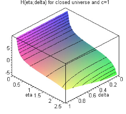
FIG. 1.: Fractional Hubble parameter calculated according to the formula (41).

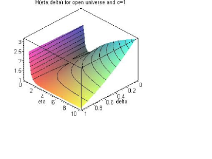
FIG. 2.: Fractional Hubble parameter calculated according to the formula (43).

REFERENCES

• [1] Ross B 1997 Lecture Notes in Mathematics 457 (Springer)
• [2] Spanier J and Oldham K B 1974 The Fractional Calculus (Academic Press) For recent reviews, see Metzler R and Klafter J 2000 Phys. Rep. 339 1 Hilfer R ed. 2000 Applications of Fractional Calculus in Physics (World Scientific)
• [3] Barkai E 2001 Phys. Rev. E 63 046118 Metzler R, Barkai E and Klafter J 1999 Phys. Rev. Lett. 82 3563
• [4] Metzler R, GlΓΆckle W G and Nonnenmacher T F 1997 Fractals 4 597
• [5] Faraoni V 1999 Am. J. Phys. 67 732 [physics/9901006]
• [6] Rosu H C 2001 Mod. Phys. Lett. A 16 2029 and 2000 Mod. Phys. Lett. A 15 979 [both in gr-qc/0003108]
• [7] Podlubny I 1999 Fractional Differential Equations (Academic Press) and 2002 Fractional Calculus and Appl. Analysis 5 367 [math.CA/0110241]
• [8] Grigolini P, Rocco A and West B J 1999 Phys. Rev. E 59 2603 [cond-mat/9809075]