Mixed State Holonomies

Abstract

Sjöqvist, Pati, Ekert, Anandan, Ericsson, Oi and Vedral (Phys. Rev. Lett. 85, 2845 [2000]) have recently “provided a physical prescription based on interferometry for introducing the total phase of a mixed state undergoing unitary evolution, which has been an elusive concept in the past”. They note that “Uhlmann was probably the first to address the issue of mixed state holonomy, but as a purely mathematical problem”. We investigate possible relationships between these “experimental” and “mathematical” approaches, by examining various quantum-theoretic scenarios. We find that the two methodologies, in general, yield inequivalent outcomes.

Mathematics Subject Classifications (2000): 81Q70

Key words. Geometric phase, Berry phase, mixed states, density matrix, Bures metric, geodesic triangles, Gibbsian density matrices, Yang-Mills connection, Uhlmann phase

I Introduction

In the introductory paragraph of their recent interesting letter, Sjöqvist et al state that “Uhlmann was probably the first to address the issue of mixed state holonomy, but as a purely mathematical (emphasis added) problem. In contrast, here we provide a new formalism of the geometric phase for mixed states in the experimental (emphasis added) context of quantum interferometry” [1]. Left unaddressed there, however, was the nature of any possible relationship between the two approaches. This question merits particular attention since Dittmann has “shown that the connection form (gauge field) related to the generalization of the Berry phase to mixed states proposed by Uhlmann satisfies the source-free Yang-Mills equation $*D*D\omega=0$, where the Hodge operator is taken with respect to the Bures metric on the space of finite-dimensional nondegenerate density matrices” [2]. This fact, Dittmann and Uhlmann noted, “may be seen as an extension to mixed states of numerous examples relating the original Berry phase to Dirac monopoles, and the Wilczek and Zee phase, to instantons” [3, sec. 1]. In their work, Sjöqvist et al do express the geometric phase in terms of an average connection form [1, eq. (16)] (for which no Yang-Mills characterization has been given). Zee has reported that the non-Abelian gauge structure associated with nuclear quadrupole resonance does not satisfy the source-free Yang-Mills equation [4] (cf. [5]). In [6], in line with certain work of Figueroa-O’Farrill concerning calibrated geometries [7, sec. 6], we have begun a study of the “Dittmann-Bures/Yang-Mills” field over the eight-dimensional convex set of three-level density matrices (making use of the formulas for the Bures metric developed in [8], based on the parameterization in [9]) by finding certain self-dual four-forms ($\varphi$) with respect to the Bures metric. The eigenspace decomposition of the associated endomorphism $\hat{\varphi}$ was found to yield four octets and three singlets as factors [6].

The research presented below represents our effort to gain a formal understanding of the relations between the “mathematical” methodology of Uhlmann and the “experimental” approach of Sjöqvist et al. We hope that this will prove useful, among other things, in the devising of a physical scheme for implementing the concepts of Uhlmann (cf. [10, sec. 4]).

In the interferometric/experimental case [1], each pure state that diagonalizes the initial density matrix ($\rho(0)$) is parallel transported separately from other distinct diagonalizing pure states, so one simply weights or (incoherently) averages the individual pure state (single-state) interference profiles by the corresponding eigenvalues of $\rho(0)$ to obtain the mixed state results . In the notation of [1], the total geometric phase is the argument of $\sum_{k}w_{k}\nu_{k}e^{i\phi_{k}}$, and the visibility is its absolute value, where $w_{k},\nu_{k},\phi_{k}$ are, respectively, the eigenvalue, visibility and geometric phase obtained for the $k$-th constituent pure state of $\rho(0)$ [1, eqs. (10), (15)]. The phase introduced by Sjöqvist et al “fulfills two central properties that make it a natural generalization of the pure state case: (i) it gives rise to a linear shift of the interference oscillations produced by a variable $U(1)$ phase and (ii) it reduces to the Pancharatnam connection for pure states” [1]. The mixed state generalization of Pancharatnam’s connection — which asserts that $\rho(t)$ and $\rho(t+dt)$ are in phase if $\mbox{Tr}[\rho(t)U(t+dt)\dagger{U}(t)]$ is real and positive — can be met only when [1, eq. (12)]

$$\mbox{Tr}[\rho(t)\dot{U}(t){U}^{\dagger}(t)]=0.$$ (1)

This is the parallel transport condition of Sjöqvist et al for mixed states undergoing unitary evolution.

In the approach of Uhlmann [11] the parallel transport takes place in a larger Hilbert space, defined by purification. The geometric phase of Sjöqvist et al can also be understood using purification [1], though the unitary operator that acts on the ancilla or auxiliary state there is unconstrained and can in fact be anything, such as the identity operator. A “parallel transport of a density operator amounts to a parallel transport of any (emphasis added) of it purifications [1, p. 2848].

In infinitesimal form, the parallelity condition of Uhlmann for a density matrix $\rho(t)$ reads [10, eq. (19)],

$$\dot{W(t)^{\dagger}}W(t)=\mbox{hermitian},$$ (2)

where $W(t)=\sqrt{\rho(t)}V(t)$. The unitary operator $V(t)$ can be interpreted as acting on the ancilla in the purification of $\rho(t)$ and is determined by this parallelity condition (2). For example, if the system, initially in the state $\rho(0)$, evolves unitarily under the evolution operator $U(t)$ one may write $W(t)=U(t)\sqrt{\rho(0)}V(t)$. The Uhlmann parallelity condition, then, reads

$$\sqrt{\rho(0)}U^{\dagger}(t)\dot{U}(t)\sqrt{\rho(0)}=V(t)\dot{V}(t)^{\dagger}\rho(0)+\rho(0)V(t)\dot{V}(t)^{\dagger}.$$ (3)

With given input $\rho(0)$ and $U(t)$ this equation needs to be solved for $V(t)$. The geometric phase $\gamma_{g}$ for any specific $T$ can then be computed using the mixed state Pancharatnam connection [1],

$$\gamma_{g}(T)=\arg\mbox{Tr}(V^{\dagger}(T)\sqrt{\rho(0)}U^{\dagger}(T)\sqrt{\rho(0)}).$$ (4)

In the three sets of analyses reported below (sec. II), we will implement certain formulas of Uhlmann [11, 12]. We compare the two methodologies under consideration in the context of: (a) unitary evolution over geodesic spherical triangles, the vertices of which are associated with certain specific mixed two-level systems; (b) unitary evolution of such two-level systems over certain circular paths ($O(3)$-orbits); and (c) unitary evolution over such circular paths of $k$-level Gibbsian density matrices [12, 13]. In case (a) we find an interesting correspondence between the two approaches for mixed states having Bloch vectors of length $\sqrt{{2\over 3}}$ and in (c) that the results of the Uhlmann methodology converge to those of Sjöqvist et al if a certain variable (a), a function ($\mbox{sech}{\alpha\over 2}$) of the inverse temperature parameter ($\alpha$), is driven to zero. If instead of strictly mixed states, we consider the unitary evolution of pure states, then both methodologies simply reproduce the corresponding Berry phase for each of the three scenarios. However, for general mixed states, the two methodologies typically yield inequivalent results.

II Analyses

A Unitary evolution over geodesic spherical triangles

For a qubit (a spin-${1\over 2}$ particle), whose density matrix can be written as,

$$\rho(0)={1\over 2}(1+r\mathbf{\hat{r}}\cdot\mathbf{\sigma}),$$ (5)

where $\mathbf{\hat{r}}$ is a unit vector, $r$ is the constant (length of the Bloch vector) for unitary evolution and $\mathbf{\sigma}$ is a vector of the three (non-identity) Pauli matrices, Sjöqvist et al obtained a formula for the geometric phase [1, eq. (25)],

$$\gamma_{g}[\Gamma]=-\mbox{arctan}\Big{(}r\mbox{tan}{\Omega\over 2}\Big{)}.$$ (6)

Here $\Gamma$ is the unitary curve in parameter space traversed by the system and $\Omega$ the solid angle subtended by the natural extension of $\Gamma$ to the unit (Bloch) sphere. This formula reduces to $-{\Omega\over 2}$ for pure states ($r=1$), as it, of course, should. The visibility was expressed as [1, eq. (26)],

$$\nu=\eta\sqrt{\cos^{2}{\Omega\over 2}+r^{2}\sin^{2}{\Omega\over 2}}.$$ (7)

For the case of cyclic evolution, which will be our only area of concern here, $\eta=1$.

We focus on the case of cyclic evolution for geodesic triangles, in particular, since Uhlmann has an enabling formula “relevant for the intensities”, [11, eq. (24)]

$$\sqrt{a_{12}a_{23}a_{31}}\mbox{Tr}\rho(0)U=r^{4}a_{321}+r^{3}(1-r){a_{12}+a_{23}+a_{31}+2a_{321}-3\over 2}+$$ (8)

$$+r^{2}(1-r)^{2}{a_{12}+a_{23}+a_{31}+6\over 2}+4r(1-r)^{3}+(1-r)^{4}.$$

Here

$$a_{12}:=\langle 1|2\rangle\langle 2|1\rangle,\quad a_{321}=\langle 3|2\rangle\langle 2|1\rangle\langle 1|3\rangle,\ldots,$$ (9)

where $|j\rangle\langle j|$ gives the projection operator $P_{j}$ associated with the $j$-th density matrix ($\tilde{\rho}_{j}$) in the geodesic triangle, that is,

$$P_{j}={2\tilde{\rho}_{j}-(1-r)\underline{1}\over 2r}.$$ (10)

Uhlmann also apparently has an explicit formula for geodesic quadrangles, but only the leading terms of it have been published [11, eq. (25)], that is,

$$\sqrt{a_{12}a_{23}a_{34}a_{41}}\mbox{Tr}\rho(0)U=r^{5}a_{4321}+$$ (11)

$$+r^{4}(1-r){6a_{4321}-a_{432}-a_{421}+3a_{431}+3a_{321}+a_{43}+a_{21}+a_{41}+a_{23}+a_{42}-3a_{13}+2\over 2}+\ldots.$$

Without loss of generality, let us set one of the three vertices of the geodesic spherical triangle swept out by the unit vector $\mathbf{\hat{r}}$ (5) in the unitary evolution to be (0,0,1). We use the standard spherical coordinate form for a point on the sphere, that is $(\sin{\theta}\cos{\phi},\sin{\theta}\sin{\phi},\cos{\theta})$, and take the other two vertices to be parameterized by the angular pairs $(\theta_{1},\phi_{1})$ and $(\theta_{2},\phi_{2})$, so the preassigned vertex (0,0,1) corresponds simply to $\theta_{1}=0$. Then, using the notation $\bar{\phi}=\phi_{1}-\phi_{2}$, we have for the solid angle [14],

$$\Omega=-2\mbox{arccot}\Big{(}\cot{\bar{\phi}}+(\cot{\theta_{1}}+\csc{\theta_{1})}(\cot{\theta_{2}}+\csc{\theta_{2}})\csc{\bar{\phi}}\Big{)}.$$ (12)

(This formula, as well as all the succeeding ones here, depend implicitly or explicitly upon $\bar{\phi}$ and not on $\phi_{1}$ and $\phi_{2}$ individually.) Let us also denote

$$\mu=(1+\cos{\theta_{1}})(1+\cos{\theta_{2}})+\cos{\bar{\phi}}\sin{\theta_{1}}\sin{\theta_{2}}.$$ (13)

The parameter $\mu$ is confined to the range $[-{1\over 2},4]$, for $0\leq\theta_{1},\theta_{2}\leq\pi,\quad 0\leq\phi_{1},\phi_{2}<2\pi$. It is equal to its minimum -${1\over 2}$ at $\theta_{1}=\theta_{2}={2\pi\over 3}$ and $\bar{\phi}=\pi$; equal to its maximum 4 for $\theta_{1}=\theta_{2}=0$ and equal to zero if either $\theta_{i}=\pi$ or $\theta_{2}=\pi$.

Making use of (8) and (9), we have for the “Uhlmann geometric phase” for the general geodesic triangle specified that

$$\tilde{\gamma}_{g}=\mbox{arg}(\mbox{Tr}\rho_{1}U)=\mbox{arctan}\Big{(}{\alpha\over\beta}\Big{)},$$ (14)

where

$$\alpha=r^{3}\sin{\bar{\phi}}\sin{\theta_{1}}\sin{\theta_{2}},\qquad\beta=4+(\mu-10)r^{2}+6r^{4}.$$ (15)

We found that

$$\tan{{\Omega\over 2}}=-{\alpha\over\mu r^{3}},$$ (16)

so one can write (6)

$$\gamma_{g}=-\mbox{arctan}\Big{(}r\tan{{\Omega\over 2}}\Big{)}=\mbox{arctan}\Big{(}{\alpha\over\mu r^{2}}\Big{)},$$ (17)

as well as

$$\tilde{\gamma}_{g}=\mbox{arctan}\Big{(}{\alpha\over\beta}\Big{)}=\mbox{arctan}\Big{(}{-\mu r^{3}\tan{{\Omega\over 2}}\over\beta}\Big{)}.$$ (18)

Let us note the exact relations between the two forms (“mathematical” and “experimental”) of geometric phase,

$${\mbox{tan}\Big{(}\gamma_{g}\Big{)}\over\mbox{tan}\Big{(}\tilde{\gamma}_{g}\Big{)}}=1+{4-10r^{2}+6r^{4}\over\mu r^{2}}=1+{\beta-\mu r^{2}\over\mu r^{2}}={\beta\over\mu r^{2}},$$ (19)

which are unity for both $r=1$ and $r=\sqrt{{2\over 3}}$. (Anandan et al [15] assert that “a fully gauge-invariant description of the geometric phase requires that it be defined modulo $2\pi$”. Of course, $\tan{\psi}=\tan{(\psi+\pi)}$.) For $r=1-\triangle r$,

$${\tan{\gamma_{g}}\over\tan{\tilde{\gamma}_{g}}}\approx\Big{(}1-{4\triangle r\over\mu}\Big{)}.$$ (20)

For $r=\sqrt{{2\over 3}}+\triangle r$,

$${\tan{\gamma_{g}}\over\tan{\tilde{\gamma}_{g}}}\approx\Big{(}1-{2\sqrt{6}\triangle r\over\mu}\Big{)}.$$ (21)

For $r=\triangle r$ (that is, a neighborhood of the fully mixed [classical] state, $r=0$),

$${\gamma_{g}\over\tilde{\gamma}_{g}}\approx{\tan{\gamma_{g}}\over\tan{\tilde{\gamma}_{g}}}\approx 1+{4-10\triangle^{2}r\over\mu\triangle^{2}r}.$$ (22)

The “Uhlmann visibility” is

$$\tilde{\nu}=|\mbox{Tr}\rho_{1}U|=\sqrt{{\alpha^{2}+\beta^{2}\over(\alpha/r^{3})^{2}+\mu^{2}}},$$ (23)

which is precisely unity for $r=1$, as is also the case for $\nu$, given by (7). Now,

$${\nu\over\tilde{\nu}}={1\over r^{2}}\sqrt{{\alpha^{2}+\mu^{2}r^{4}\over\alpha^{2}+\beta^{2}}}.$$ (24)

This ratio is always unity for $r=1$ and always ${3\over 2}$ for $r=\sqrt{{2\over 3}}$. (Recall, on the other hand, that the ratio (19) of the tangents of the two geometric phases is unity for $r=\sqrt{{2\over 3}}$.) For $r=1-\triangle r$,

$${\nu\over\tilde{\nu}}\approx 1+\triangle r\Big{(}2+{4\mu\over(\alpha/r^{3})^{2}+\mu^{2}}\Big{)}.$$ (25)

For $r=\sqrt{{2\over 3}}+\triangle r$,

$${\nu\over\tilde{\nu}}\approx{3\over 2}\Big{(}1+\sqrt{6}\triangle r({6\mu\over 2(\alpha/r^{3})^{2}+3\mu^{2}}-1)\Big{)}.$$ (26)

For $r=\triangle r$,

$${\nu\over\tilde{\nu}}\approx{\mu\over 4}+\triangle^{2}r\Big{(}{(\alpha/r^{3})^{2}\over 8\mu}-{1\over 16}(\mu-10)\mu\Big{)}.$$ (27)

In the limit $r\rightarrow 0$,

$${\nu\over\tilde{\nu}}={\mu\over 4}.$$ (28)

B Unitary evolution over certain circular paths

Now let us similarly study the unitary evolution of spin-${1\over 2}$ systems over circular ($O(3)$-orbits) — as opposed to geodesic triangular — paths. We utilize the analyses of Uhlmann in [12]. Again, we start with an initial density matrix $\rho(0)$, the Bloch vector of which is proportional to (0,0,1), while the axis of rotation about which the state evolves is $\overrightarrow{n}=(0,\sin{\xi},\cos{\xi})$. The resulting curve of density matrices is given by

$$\phi\rightarrow U(\phi)\rho(0)U(-\phi),\qquad U(\phi)=e^{-i\phi(\sin{\xi}J_{y}+\cos{\xi}J_{z})},$$ (29)

and the associated parallel lift of this curve with initial value ${\rho(0)}^{1/2}$ by

$$\phi\rightarrow U(\phi){\rho(0)}^{1/2}V(\phi),\qquad V(\phi)=e^{i\phi(\sin{\xi}\hat{J}_{y}+\cos{\xi}J_{z})},$$ (30)

where

$$2\rho(0)^{1/2}J_{y}\rho(0)^{1/2}=\rho(0)\hat{J}_{y}+\hat{J}_{y}\rho(0),$$ (31)

and the $J$’s are, of course, generators of an irreducible representation of $SU(2)$. We have the relation

$$\xi=\cos^{-1}{\Big{(}-{\Omega\over 2\pi}\Big{)}}.$$ (32)

The associated holonomy invariant for a complete rotation about $\overrightarrow{n}$ is

$$\rho(0)^{1/2}U(2\pi)V(2\pi)\rho(0)^{1/2}.$$ (33)

(In [13, sec. V], we have studied certain “higher-order” holonomy invariants.) We then have the result (using the “$\quad\breve{}\quad$” notation now, rather than “$\quad\tilde{}\quad$” as before, to refer to results obtained based on the unitary circular evolution analysis of Uhlmann [12])

$${\tan{\gamma_{g}}\over\tan{\breve{\gamma}_{g}}}=\chi\sec{\xi}\coth{\pi\chi}\tan{(\pi\cos{\xi})}={\pi\chi\tan{\kappa}\coth{\pi\chi}\over\kappa},$$ (34)

where

$$\chi=\sqrt{{r^{2}-2-r^{2}\cos{2\xi}\over 2}},$$ (35)

and

$$\kappa={\pi\sqrt{-1+r^{2}-\chi^{2}}\over r}=\pi\cos{\xi}=-{\Omega\over 2}.$$ (36)

We plot this ratio (34) in Fig. 1.

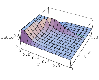
FIG. 1.: Ratio (34) of tangents of geometric phases for unitary evolution over circular paths

Now for $\triangle\xi$,

$${\tan{\gamma_{g}}\over\tan{\breve{\gamma}_{g}}}\approx{4+3(1-r^{2})(\triangle\xi)^{2}\over 4r^{2}}.$$ (37)

For pure states ($r=1$), the ratio (34) reduces to 1. The ratio of the visibilities,

$${\nu\over\breve{\nu}}={\chi\sqrt{2}\sqrt{\cos^{2}{\kappa}+r^{2}\sin^{2}{\kappa}}\over\sqrt{1-r^{2}+2\chi^{2}+(r^{2}-1)\cosh{2\pi\chi}}}={\chi\sqrt{2}\sqrt{\cos^{2}{\kappa}+(1+\chi^{2})\csc^{2}{\xi}\sin^{2}{\kappa}}\over\sqrt{1+2\chi^{2}-\cosh{2\pi\chi}+2(1+\chi^{2})\csc^{2}{\xi}\sinh^{2}{\pi\chi}}},$$ (38)

is given in Fig. 2. Both the ratios (34) and (38) are unity for pure states ($r=1$).

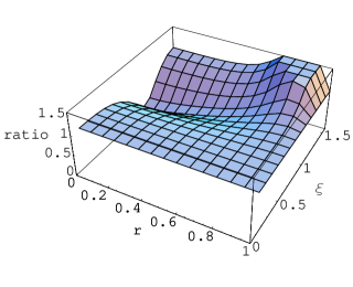
FIG. 2.: Ratio (38) of visibilities for unitary evolution over circular paths

C Unitary evolution of Gibbsian $k$-level density matrices

In the final part of the paper [12], Uhlmann also considered the analogous unitary circular evolution ($O(3)$-orbits) of $k$-level Gibbsian states of the form

$$\rho={e^{\alpha\overrightarrow{n}\overrightarrow{J}}\over\mbox{trace}\quad e^{\alpha\overrightarrow{n}\overrightarrow{J}}},$$ (39)

where the vector $\overrightarrow{J}$ of angular momentum operators lives in $k$-dimensions. (For $k=2$, the model is equivalent to that studied in the previous section.) In [13] we have conducted a detailed analysis of this model in comparison with the results that would be obtained implementing the methodology of Sjöqvist et al. One unanticipated outcome was that the Sjöqvist et al model appeared sensitive to the bosonic (odd $k$) or fermionic (even $k$) nature of the $k$-level systems. As an example of this phenomenon, we exhibit two additional plots (Fig. 3 and 4) based on analyses for $k=2,\ldots,11$. In each of these plots, the inverse temperature parameter $\alpha$ is held fixed at 2. In Fig. 3, based on the Uhlmann methodology, below $\xi\approx.65$ the ten curves are all monotonically decreasing. The order of dominance among themselves of these curves is the natural order $k=2,\ldots,11$, with the curve for $k=2$ being the dominant one. On the other hand, using the procedure of Sjöqvist et al, the ten corresponding curves are separated into two clusters of five (below $\xi\approx.44$) (Fig. 3). In the first cluster (having the higher values of $\gamma$) in decreasing order of dominance the five curves correspond to $k=2,4,6,8,10$, while in the second group (having lesser values) the order is $k=3,5,7,9,11$. (For other related Figures, see [13, sec. VIII].)

FIG. 3.: Geometric phases, based on the Uhlmann methodology, for the $k$-level Gibbsian density matrices, holding the inverse temperature parameter $\alpha$ fixed at 2. Below $\xi\approx.65$, the curve for $k=2$ dominates that for $k=3$, which dominates that for $k=4,\ldots$

FIG. 4.: Geometric phases, based on the Sjöqvist et al methodology, for the $k$-level Gibbsian density matrices, holding the inverse temperature parameter $\alpha$ fixed at 2. Below $\xi\approx.45$, the upper (even $k$) group of curves in decreasing order of dominance correspond to $k=2,4,6,8,10$ and the lower (odd $k$) group to $k=3,5,7,9,11$

Also, we have found [13] that the (first-order) holonomy invariant in the Uhlmann approach [12, eqs. (33), (43), (47)], that is the trace of

$$W(2\pi)W(0)^{\dagger}=(-1)^{2j}\rho(0)^{1/2}e^{2\pi i(\cos{\theta}J_{z}+a\sin{\theta}J_{y})}\rho(0)^{1/2},$$ (40)

reduces to $(-1)^{k+1}$ times the holonomy invariant [1, eq. (15)] in the Sjöqvist et al analysis if we simply set the parameter $a=\mbox{sech}{\alpha\over 2}$ in (40) to zero, that is the influence of the angular momentum operator $J_{y}$ is nullified. Relatedly, if $\rho(0)$ were the density matrix of a pure state, then the term $a\sin{\theta}J_{y}$ in the invariant (40) would drop out, with the trace of the resultant expression being the corresponding Berry phase [12, eq. (43)]. This fact was employed in [13] to compute the Sjöqvist et al mixed state holonomy for the $k$-level Gibbsian density matrices, by taking the average (using the eigenvalues of $\rho(0)$ as weights) of these Berry phases for the pure states that diagonalize the initial density matrix [1, eqs. (10), (15)].

III Concluding Remarks

The analyses presented above clearly demonstrate a general inequivalence between the “experimental” approach to mixed state holonomy of Sjöqvist et al [1] and the “purely mathematical” scheme of Uhlmann [11, 12]. In particular, in the third of our analyses (sec. II C), concerned with $O(3)$-orbits of $k$-level Gibbsian density matrices, it has emerged that the analyses of Sjöqvist et al (Fig. 4) are sensitive to the parity of $k$, while those of Uhlmann (Fig. 3) are not [13]. (For an application of [1] to the detection of quantum entanglement, see [16]. For a further discussion of the results in [1], see [10, secs. 2, 4].)

A problem that remains to be fully addressed is the conceptualization of a physical apparatus that would yield the geometric phases and visibilities given by the analyses of Uhlmann [11, 12]. In their study [1], Sjöqvist et al did describe the use of a Mach-Zehnder interferometer to “test the geometric phase for mixed states and provide the notion of phase and parallel transport for mixed states in a straightforward way”. However, they did not specify such a physical scheme for their conceptual alternative based on a purification procedure (cf. [10, sec. 4]).

Let us also note that the connection used for parallel transport in the Uhlmann (Bures) case is but one of an (uncountable) infinite set of connections (“defining reasonable parallel transports along curves of density operators”), which correspond in a one-to-one fashion, with the monotone metrics on the $k$-level density matrices, and are all compatible with the purification procedure [3, 17, 18]. In this generalized framework, the Uhlmann (canonical) connection corresponds to the well-studied Bures or minimal monotone metric [2, 19]. A yet apparently formally unsettled question is whether or not the Sjöqvist et al connection [1, eqs. (16)-(18)] itself corresponds to some such monotone metric, thus falling within this generalized scheme of Dittmann and Uhlmann of connections (and metrics) respecting standard purification [3]. From the results presented above, it is clear that it does not correspond to the Bures metric. (In the Uhlmann methodology, “proper liftings” $W(t)$ are those that minimize the length functional $\int\mbox{Tr}\mbox{[}d\dot{W}^{*}dW]$ of the curve of density operators undergoing unitary evolution. For a proper lifting this length becomes equal to the “Bures length”. One particularly interesting property of the Bures metric is that its volume element can be employed to determine analytically exact probabilities that a pair of quantum bits is [a priori] classically correlated [20].)

- [1] Sjöqvist E., Pati, A. K., Ekert, A., Anandan, J. S., Ericsson, M., Oi, D. K. L., and Vedral, V.: Geometric phases for mixed states in interferometry. Phys. Rev. Lett. 85, 2845 (2000).
- [2] Dittmann, J.: Yang-Mills equation and Bures metric. Lett. Math. Phys. 46, 281 (1998).
- [3] Dittmann, J. and Uhlmann, A.: Connections and metrics respecting purification of quantum states. J. Math. Phys. 40, 3246 (1999).
- [4] Zee, A.: Non-Abelian structure in nuclear quadrupole resonance. Phys. Rev. A, 38, 1 (1988).
- [5] Avron, J. E., Sadun, L., Segert, J. and Simon, B.: Topological invariants in Fermi systems with time-reversal invariance. Phys. Rev. Lett. 61, 1329 (1988).
- [6] Slater, P. B.: Self-duality, four-forms, and the eight-dimensional Yang-Mills field over the three-level density matrices. e-print, math-ph/0108005.
- [7] Figueroa-O’Farrill, J. M.: Intersecting brane geometries. J. Geom. Phys. 35, 99 (2000).
- [8] Slater, P. B.: Bures geometry of the three-level quantum systems, J. Geom. Phys. 39, 207 (2001).
- [9] Byrd, M. and Slater, P. B.: Bures measures over the spaces of two and three-dimensional density matrices. Phys. Lett. A 283, 152 (2001).
- [10] Sjöqvist, E.:Pancharatnam revisted. e-print, quant-ph/0202078.
- [11] Uhlmann, A.: On cyclic evolution of mixed states in two-level systems. In Nonlinear, Dissipative, Irreversible Quantum Systems (Clausthal, 1994), edited by Doebner, H.-D., Dobrev, V. K., and Natterman, P. (World Scientific, 1995), p. 296 .
- [12] Uhlmann, A.: Parallel lifts and holonomy along density operators: computable examples using -orbits. In Symmetries in Science VI, edited by B. Gruber, (Plenum, New York, 1993), p. 741.
- [13] Slater, P. B.: Geometric phases of the Uhlmann and Sjöqvist et al types for -orbits of -level Gibbsian density matrices. e-print, math-ph/0112054.
- [14] Eriksson, F.: On the measure of solid angles. Math. Mag. 63, 184 (1990).
- [15] Anandan, J., Sjöqvist, E., Pati, A. K., Ekert, A., Ericsson, M., Oi, D. K. L., and Vedral, V.: Reply to “Singularities of the mixed state phase”. e-print, quant-ph/0109139.
- [16] Horodecki, P. and Ekert, A.: Direct detection of quantum entanglement. e-print, quant-ph/0111064.
- [17] Petz, D. and Súdar, C.: Geometries of quantum states. J. Math. Phys. 37, 2662 (1996).
- [18] Slater, P. B.: Monotonicity properties of certain measures over the two-level quantum systems. Lett. Math. Phys. 52, 343 (2000).
- [19] Dittmann, J.: Explicit formulae for the Bures metric. J. Phys. A 32, 2663 (1999).
- [20] Slater, P. B.: Exact Bures probabilities that two quantum bits are classically correlated. Eur. Phys. J.B 17, 471 (2000).