We present exact calculations of the partition function of the zero-temperature Potts antiferromagnet (equivalently, the chromatic polynomial) for graphs of arbitrarily great length composed of repeated complete subgraphs $K_{b}$ with $b=5,6$ which have periodic or twisted periodic boundary condition in the longitudinal direction. In the $L_{x}\to\infty$ limit, the continuous accumulation set of the chromatic zeros ${\cal B}$ is determined. We give some results for arbitrary $b$ including the extrema of the eigenvalues with coefficients of degree $b-1$ and the explicit forms of some classes of eigenvalues. We prove that the maximal point where ${\cal B}$ crosses the real axis, $q_{c}$, satisfies the inequality $q_{c}\leq b$ for $2\leq b$, the minimum value of $q$ at which ${\cal B}$ crosses the real $q$ axis is $q=0$, and we make a conjecture concerning the structure of the chromatic polynomial for Klein bottle strips.

I Introduction

The $q$-state Potts antiferromagnet (AF) [1, 2] exhibits nonzero ground state entropy, $S_{0}>0$ (without frustration) for sufficiently large $q$ on a given lattice $\Lambda$ or, more generally, on a graph $G$. This is equivalent to a ground state degeneracy per site $W>1$, since $S_{0}=k_{B}\ln W$. There is a close connection with graph theory here, since the zero-temperature partition function of the above-mentioned $q$-state Potts antiferromagnet on a graph $G$ satisfies

$$Z(G,q,T=0)_{PAF}=P(G,q)\ ,$$ (1)

where $P(G,q)$ is the chromatic polynomial expressing the number of ways of coloring the vertices of the graph $G$ with $q$ colors such that no two adjacent vertices have the same color (for reviews, see [3]-[5]). The minimum number of colors necessary for such a coloring of $G$ is called the chromatic number, $\chi(G)$. Thus

$$W(\{G\},q)=\lim_{n\to\infty}P(G,q)^{1/n}\ ,$$ (2)

where $n$ is the number of vertices of $G$ and $\{G\}=\lim_{n\to\infty}G$. Where no confusion will result, we shall sometimes write $G$ rather than $\{G\}$ for the infinite-length limit of a given type of strip graph. At certain special points $q_{s}$ (typically $q_{s}=0,1,..,\chi(G)$), one has the noncommutativity of limits

$$\lim_{q\to q_{s}}\lim_{n\to\infty}P(G,q)^{1/n}\neq\lim_{n\to\infty}\lim_{q\to q_{s}}P(G,q)^{1/n}\ ,$$ (3)

and hence it is necessary to specify the order of the limits in the definition of $W(\{G\},q_{s})$ [6]. Denoting $W_{qn}$ and $W_{nq}$ as the functions defined by the different order of limits on the left and right-hand sides of (3), we take $W\equiv W_{qn}$ here; this has the advantage of removing certain isolated discontinuities that are present in $W_{nq}$.

Using the expression for $P(G,q)$, one can generalize $q$ from ${\mathbb{Z}}_{+}$ to ${\mathbb{C}}$. The zeros of $P(G,q)$ in the complex $q$ plane are called chromatic zeros; a subset of these may form an accumulation set in the $n\to\infty$ limit, denoted ${\cal B}$, which is the continuous locus of points where $W(\{G\},q)$ is nonanalytic. The maximal region in the complex $q$ plane to which one can analytically continue the function $W(\{G\},q)$ from physical values where there is nonzero ground state entropy is denoted $R_{1}$. The maximal value of $q$ where ${\cal B}$ intersects the (positive) real axis is labeled $q_{c}(\{G\})$. This point is important since $W(\{G\},q)$ is a real analytic function from large values of $q$ down to $q_{c}(\{G\})$.

Here we present exact calculations of the partition function of the chromatic polynomial $P(G,q)$ for graphs of arbitrarily great length composed of repeated complete subgraphs $K_{b}$ with $b=5,6$ which have periodic or twisted periodic boundary conditions in the longitudinal direction. Thus, consider $L_{x}$ copies of the complete graph $K_{L_{y}}$ with vertex set $V(K_{L_{y}})=\{1,2,...,L_{y}\}$. Denote the edges joining each adjacent pair of $K_{L_{y}}$ and $K^{\prime}_{L_{y}}$ graphs as $L=\{v_{i}v^{\prime}_{j}|i,j=1,...,L_{y}\}$, where $v_{i},v^{\prime}_{j}$ are vertices of adjacent complete graphs $K_{L_{y}}$ and $K^{\prime}_{L_{y}}$, and impose periodic boundary conditions in the longitudinal direction, $x$. In [7], the graph with $L_{x}$ copies of $K_{L_{y}}$ for arbitrary $L_{x}$ and $L_{y}$ was called the bracelet strip. The total number of vertices is $n=L_{x}L_{y}$ for these strips.

A generic form for chromatic polynomials for recursively defined families of graphs (families of graphs that can be constructed via repeated addition of some subgraph), of which strip graphs $G_{s}$ are special cases, is [8]

$$P((G_{s})_{m},q)=\sum_{j=1}^{N_{G_{s},\lambda}}c_{G_{s},j}(q)(\lambda_{G_{s},j}(q))^{L_{x}}\ ,$$ (4)

where $c_{G_{s},j}(q)$ and the $N_{G_{s},\lambda}$ terms $\lambda_{G_{s},j}(q)$ depend on the type of strip graph $G_{s}$ but are independent of $L_{x}$.

For a given type of strip graph $G_{s}$, we denote the sum of the coefficients $c_{G_{s},j}$ as

$$C(G_{s},q)=\sum_{j=1}^{N_{G_{s},\lambda}}c_{G_{s},j}(q)\ .$$ (5)

Some works on calculations of chromatic polynomials for recursive families of graphs include [9]-[49].

II Family of toroidal Strips

Specifically, we consider the set of edges linking two successive complete graphs on the chain is $L=\{11,22,33,...,L_{y}L_{y}\}$, which will be denoted as a torus. For $L_{y}=2$, this is the ladder graph with vertex set $T_{2}=K_{2}$ [9]. For the graph with $L_{y}=3,4$, which has vertex set $C_{3}=K_{3}$ and $K_{4}$, the chromatic polynomial was given in [10] and [11], respectively. In [58, 59], these families of graphs with linking edge sets $\{11,22,33,...,bb\}$ were denoted as $B_{m}(b)$, where $b=L_{y}$, $m=L_{x}$. The corresponding Klein bottle strip is the same as the toroidal strip except one of the linking edge set is $\{1L_{y},2(L_{y}-1),...L_{y}1\}$. The form of the chromatic polynomials for the $B_{m}(b)$ strips was determined to be

$$P(B_{m}(b),q)=\sum_{d=0}^{b}\sum_{j=1}^{N_{B_{m}(b),d,\lambda}}c_{B_{m}(b),d,j}(q)c^{\prime}_{B_{m}(b),d,j}(\lambda_{B_{m}(b),d,j}(q))^{m}\ ,$$ (6)

where $d$ is the degree of the coefficient $c_{B_{m}(b),d,j}(q)$ as a polynomial in $q$, and the $c^{\prime}_{B_{m}(b),d,j}$’s are numbers which depend on $b$. The structural feature that these coefficients can be grouped into sets of fixed degree $d$ is similar to that found in [14] for cyclic strips of the square and triangular lattice, although for these bracelet chain graphs, for $b\geq 3$, there is more than one coefficient of a given degree (see [10] for the case $b=3$), whereas in contrast, for the cyclic strip graphs studied in [14] (and the self-dual family studied in [55]) there is only one coefficient of each degree. The degree $d$ is denoted as the ‘level’ in [60, 58, 59]. The $\lambda_{B_{m}(b),d,j}(q)$ is the eigenvalue of an appropriately defined transfer matrix [37] and is a polynomial in $q$ of degree $b-d$. For sufficiently large integer $q$, the coefficient $c_{B_{m}(b),d,j}(q)c^{\prime}_{B_{m}(b),d,j}$ can be interpreted as the multiplicity of this eigenvalue.

There are partitions associated with each $d$ which were used to determine the forms of $c_{B_{m}(b),d,j}$ in [59]. For a partition $X$ of $d$ such that $x_{d}+x_{d-1}+...+x_{1}=d$ and $x_{d}\leq x_{d-1}\leq...\leq x_{1}$ where $x_{i}$ for $2\leq i\leq d$ are non-negative integers and $x_{1}$ is a positive integer, there is an associated partition $Y$ of $d(d+1)/2$ such that $y_{d}+y_{d-1}+...+y_{1}=d(d+1)/2$ and $y_{i}=x_{i}+d-i$ for $1\leq i\leq d$. Then the $c_{B_{m}(b),d,j}$ for a partition $X$ can be written as

$$c_{X,d}=\frac{1}{d!}\prod_{i=1}^{d}(q-y_{i})\ .$$ (7)

For the partitions $[d]$ and $[1^{d}]$, the associated $\lambda_{B_{m}(b),d,j}(q)$’s were given in [58].

A $L_{y}=5$ toroidal strip

By using theorems in [58], we find the chromatic polynomial for $B_{m}(5)$, i.e., the $5\times L_{x}$ strips with each transverse slice forming a $K_{5}$ graph, and with edge linking set $L=\{11,22,33,44,55\}$ between two adjacent slices.

It is convenient to express the $\lambda$’s in term of the following functions [60]

$$f_{i}(b,q)=\sum_{s=0}^{b-i}(-1)^{s}{b-i\choose s}(q-i-s)^{(b-i-s)}\ ,$$ (8)

where $q^{(k)}$ is falling factorial defined as

$$q^{(k)}=\prod_{s=0}^{k-1}(q-s)\ .$$ (9)

Here we adopt the convention that $f_{i}(b,q)=0$ if $b<i$.

For the case $b=5$, one has

$$f_{0}(5,q) = q^{5}-15q^{4}+95q^{3}-325q^{2}+609q-501$$ (10)

$$f_{1}(5,q) = q^{4}-14q^{3}+77q^{2}-200q+209$$ (11)

$$f_{2}(5,q) = q^{3}-12q^{2}+50q-73$$ (12)

$$f_{3}(5,q) = q^{2}-9q+21$$ (13)

$$f_{4}(5,q) = q-5$$ (14)

$$f_{5}(5,q) = 1\ ,$$ (15)

and the chromatic polynomial for the $B_{m}(5)$ strip is

$$P(B_{m}(5),q)=\sum_{d=0}^{5}\sum_{j=1}^{N_{B_{m}(5),d,\lambda}}c_{B_{m}(5),d,j}(q)c^{\prime}_{B_{m}(5),d,j}(\lambda_{B_{m}(5),d,j}(q))^{m}\ ,$$ (16)

where $N_{B_{m}(5),d,\lambda}$’s are equal to $1,2,5,9,9,1$ for $d$ from $0$ to $5$. We find that the total number of distinct $\lambda$’s is

$$N_{P,B_{m}(5),\lambda}=\sum_{d=0}^{5}N_{B_{m}(5),d,\lambda}=27\ .$$ (17)

We note that our result (17) differs from the pattern $N_{P,B_{m}(b),\lambda}=2^{b}$ that was found for $1\leq b\leq 4$, namely $N_{P,B_{m}(1),\lambda}=2$, $N_{P,B_{m}(2),\lambda}=2^{2}$ [9], $N_{P,B_{m}(3),\lambda}=2^{3}$ [10], and $N_{P,B_{m}(4),\lambda}=2^{4}$ [11].

We calculate that the eigenvalue with coefficient of degree 0 in $q$ is unique and is given by

$$\lambda_{B_{m}(5),0,1}=f_{0}(5,q)=q^{5}-15q^{4}+95q^{3}-325q^{2}+609q-501\ .$$ (18)

For the eigenvalues with coefficients of degree 1 in $q$ we find

$$\lambda_{B_{m}(5),1,1}=-f_{1}(5,q)+4f_{2}(5,q)=-q^{4}+18q^{3}-125q^{2}+400q-501$$ (19)

$$\lambda_{B_{m}(5),1,2}=-f_{1}(5,q)-f_{2}(5,q)=-(q-4)(q^{3}-9q^{2}+29q-34)\ .$$ (20)

Next, for the eigenvalues with coefficients of degree 2 in $q$ we obtain

$$\lambda_{B_{m}(5),2,1}=f_{2}(5,q)-6f_{3}(5,q)+6f_{4}(5,q)=q^{3}-18q^{2}+110q-229$$ (21)

$$\lambda_{B_{m}(5),2,2}=f_{2}(5,q)-f_{3}(5,q)-4f_{4}(5,q)=q^{3}-13q^{2}+55q-74$$ (22)

$$\lambda_{B_{m}(5),2,3}=f_{2}(5,q)+2f_{3}(5,q)+2f_{4}(5,q)=q^{3}-10q^{2}+34q-41$$ (23)

$$\lambda_{B_{m}(5),2,4}=f_{2}(5,q)-3f_{3}(5,q)=q^{3}-15q^{2}+77q-136$$ (24)

$$\lambda_{B_{m}(5),2,5}=f_{2}(5,q)+2f_{3}(5,q)=q^{3}-10q^{2}+32q-31\ .$$ (25)

For $1\leq j\leq 3$ these $\lambda_{B_{m}(5),2,j}$’s correspond to the partition $[2]$ and for $j=4,5$ to the partition $[11]$.

Proceeding to the eigenvalues with coefficients of degree 3, we find

$$\lambda_{B_{m}(5),3,1}=-f_{3}(5,q)+6f_{4}(5,q)-6f_{5}(5,q)=-q^{2}+15q-57$$ (26)

$$\lambda_{B_{m}(5),3,2}=-f_{3}(5,q)+f_{4}(5,q)+4f_{5}(5,q)=-q^{2}+10q-22$$ (27)

$$\lambda_{B_{m}(5),3,3}=-f_{3}(5,q)-2f_{4}(5,q)-2f_{5}(5,q)=-q^{2}+7q-13$$ (28)

$$\lambda_{B_{m}(5),3,4}=-f_{3}(5,q)+4f_{4}(5,q)-2f_{5}(5,q)=-q^{2}+13q-43$$ (29)

$$\lambda_{B_{m}(5),3,5}=-f_{3}(5,q)+f_{4}(5,q)+f_{5}(5,q)=-(q-5)^{2}$$ (30)

$$\lambda_{B_{m}(5),3,6}=-f_{3}(5,q)-f_{4}(5,q)+3f_{5}(5,q)=-q^{2}+8q-13$$ (31)

$$\lambda_{B_{m}(5),3,7}=-f_{3}(5,q)-3f_{4}(5,q)-3f_{5}(5,q)=-(q-3)^{2}$$ (32)

$$\lambda_{B_{m}(5),3,8}=-f_{3}(5,q)+2f_{4}(5,q)=-q^{2}+11q-31$$ (33)

$$\lambda_{B_{m}(5),3,9}=-f_{3}(5,q)-3f_{4}(5,q)=-q^{2}+6q-6\ .$$ (34)

Here the $\lambda_{B_{m}(5),3,j}$ for $1\leq j\leq 3$ correspond to the partition $[3]$, for $4\leq j\leq 7$ to the partition $[21]$, and for $j=8,9$ to the partition $[111]$.

For the eigenvalues with coefficients of degree 4 in $q$, we calculate

$$\lambda_{B_{m}(5),4,1}=f_{4}(5,q)-4f_{5}(5,q)=q-9$$ (35)

$$\lambda_{B_{m}(5),4,2}=f_{4}(5,q)+f_{5}(5,q)=q-4$$ (36)

$$\lambda_{B_{m}(5),4,3}=f_{4}(5,q)-3f_{5}(5,q)=q-8$$ (37)

$$\lambda_{B_{m}(5),4,4}=f_{4}(5,q)+3f_{5}(5,q)=q-2$$ (38)

$$\lambda_{B_{m}(5),4,5}=f_{4}(5,q)+2f_{5}(5,q)=q-3$$ (39)

$$\lambda_{B_{m}(5),4,6}=f_{4}(5,q)=q-5$$ (40)

$$\lambda_{B_{m}(5),4,7}=f_{4}(5,q)-2f_{5}(5,q)=q-7$$ (41)

$$\lambda_{B_{m}(5),4,8}=f_{4}(5,q)-f_{5}(5,q)=q-6$$ (42)

$$\lambda_{B_{m}(5),4,9}=f_{4}(5,q)+4f_{5}(5,q)=q-1\ .$$ (43)

Here the $\lambda_{B_{m}(5),4,j}$ for $j=1,2$ correspond to the partition $[4]$, for $j=3,5,6$ to the partition $[31]$, for $j=4,6,7$ to the partition $[211]$, for $j=5,7$ to the partition $[22]$, and for $j=8,9$ to the partition $[1111]$. Notice that the terms $\lambda_{B_{m}(5),4,j}$ for $5\leq j\leq 7$ involve degeneracies from two different associated partitions.

Finally, for the eigenvalue with coefficient of degree 5, we have

$$\lambda_{B_{m}(5),5,1}=-f_{5}(5,q)=-1\ .$$ (44)

This involves a degeneracy from all the possible partitions.

The coefficient $c_{B_{m}(5),d,j}(q)c^{\prime}_{B_{m}(5),d,j}$ of degree 0 in $q$ is

$$c_{B_{m}(5),0,1}c^{\prime}_{B_{m}(5),0,1}=1\ .$$ (45)

The coefficients of degree 1 in $q$ are

$$c_{B_{m}(5),1,1}c^{\prime}_{B_{m}(5),1,1}=q-1$$ (46)

$$c_{B_{m}(5),1,2}c^{\prime}_{B_{m}(5),1,2}=4(q-1)\ ,$$ (47)

where $c_{B_{m}(5),1,j}=q-1$ for $j=1,2$, and $c^{\prime}_{B_{m}(5),1,j}=1,4$ for $j=1,2$.

For $d=2$, there are partitions $[2]$ and $[11]$, and the associated $c_{X,2}$ are $c_{[2],2}=\frac{1}{2}q(q-3)$ and $c_{[11],2}=\frac{1}{2}(q-1)(q-2)$. The coefficients of degree 2 in $q$ are listed in Table I

TABLE I.: Coefficients of degree 2 in $q$ for $B_{m}(5)$ strip.

$j$	partition	$c^{\prime}_{B_{m}(5),2,j}$	$c_{B_{m}(5),2,j}c^{\prime}_{B_{m}(5),2,j}$
1	[2]	1	$\frac{1}{2}q(q-3)$
2	[2]	4	$2q(q-3)$
3	[2]	5	$\frac{5}{2}q(q-3)$
4	[11]	4	$2(q-1)(q-2)$
5	[11]	6	$3(q-1)(q-2)$

For $d=3$, there are partitions $[3]$, $[21]$ and $[111]$, and the associated $c_{X,3}$ are $c_{[3],3}=\frac{1}{6}q(q-1)(q-5)$, $c_{[21],3}=\frac{1}{6}q(q-2)(q-4)$ and $c_{[111],3}=\frac{1}{6}(q-1)(q-2)(q-3)$. The coefficients of degree 3 in $q$ are listed in Table II

TABLE II.: Coefficients of degree 3 in $q$ for $B_{m}(5)$ strip.

$j$	partition	$c^{\prime}_{B_{m}(5),3,j}$	$c_{B_{m}(5),3,j}c^{\prime}_{B_{m}(5),3,j}$
1	[3]	1	$\frac{1}{6}q(q-1)(q-5)$
2	[3]	4	$\frac{2}{3}q(q-1)(q-5)$
3	[3]	5	$\frac{5}{6}q(q-1)(q-5)$
4	[21]	8	$\frac{4}{3}q(q-2)(q-4)$
5	[21]	10	$\frac{5}{3}q(q-2)(q-4)$
6	[21]	12	$2q(q-2)(q-4)$
7	[21]	10	$\frac{5}{3}q(q-2)(q-4)$
8	[111]	6	$(q-1)(q-2)(q-3)$
9	[111]	4	$\frac{2}{3}(q-1)(q-2)(q-3)$

For $d=4$, there are partitions $[4]$, $[31]$, $[22]$, $[211]$ and $[1111]$, and the associated $c_{X,4}$ are $c_{[4],4}=\frac{1}{24}q(q-1)(q-2)(q-7)$, $c_{[31],4}=\frac{1}{24}q(q-1)(q-3)(q-6)$, $c_{[22],4}=\frac{1}{24}q(q-1)(q-4)(q-5)$, $c_{[211],4}=\frac{1}{24}q(q-2)(q-3)(q-5)$, and $c_{[1111],4}=\frac{1}{24}(q-1)(q-2)(q-3)(q-4)$. The coefficients of degree 4 in $q$ are listed in Table III

TABLE III.: Coefficients of degree 4 in $q$ for $B_{m}(5)$ strip.

$j$	partition	$c^{\prime}_{B_{m}(5),4,j}$	$c_{B_{m}(5),4,j}c^{\prime}_{B_{m}(5),4,j}$
1	[4]	1	$\frac{1}{24}q(q-1)(q-2)(q-7)$
2	[4]	4	$\frac{1}{6}q(q-1)(q-2)(q-7)$
3	[31]	12	$\frac{1}{2}q(q-1)(q-3)(q-6)$
4	[211]	12	$\frac{1}{2}q(q-2)(q-3)(q-5)$
5	[31]	18	$\frac{1}{6}q(q-1)(7q^{2}-63q+131)$
	[22]	10
6	[31]	15	$\frac{5}{4}q(q-3)(q^{2}-7q+8)$
	[211]	15
7	[211]	18	$\frac{1}{6}q(q-5)(7q^{2}-35q+37)$
	[22]	10
8	[1111]	4	$\frac{1}{6}(q-1)(q-2)(q-3)(q-4)$
9	[1111]	1	$\frac{1}{24}(q-1)(q-2)(q-3)(q-4)$

Finally, the coefficient of degree 5 in $q$ is given by

$$c_{B_{m}(5),5,1}c^{\prime}_{B_{m}(5),5,1}=q^{5}-15q^{4}+75q^{3}-145q^{2}+89q-1\ .$$ (48)

The sum of all the coefficients is equal to

$$C(B_{m}(5),q) = \sum_{d=0}^{5}\sum_{j=1}^{N_{B_{m}(5),d,\lambda}}c_{B_{m}(5),d,j}(q)c^{\prime}_{B_{m}(5),d,j}$$ (49)

$$= q(q-1)(q-2)(q-3)(q-4)=P(K_{5},q)\ .$$ (50)

The chromatic number is $\chi(B_{m}(5))=5$.

The locus ${\cal B}$ and chromatic zeros for the $B_{m}(5)$ strip with $L_{x}=m=20$ are shown in Fig. 1. The locus ${\cal B}$ crosses the real $q$-axis at $q=0,2,4$ and $q_{c}(B_{m}(5))$, where

$$q_{c}(B_{m}(5))\simeq 4.50634\cdots\ .$$ (51)

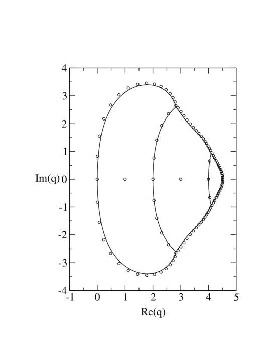
FIG. 1.: Locus ${\cal B}$ for the $m\to\infty$ limit of the family $B_{m}(5)$ with toroidal boundary conditions and chromatic zeros for $B_{m}(5)$ with $m=20$ (i.e., $n=100$).

The locus ${\cal B}$ has support for $Re(q)\geq 0$, and separates the $q$ plane into four regions. The outermost one, region $R_{1}$, extends to infinite $|q|$ and includes the intervals $q\geq q_{c}(B_{m}(5))$ and $q\leq 0$ on the real $q$ axis. Region $R_{2}$ includes the real interval $4\leq q\leq q_{c}(B_{m}(5))$, region $R_{3}$ includes the real interval $2\leq q\leq 4$, while region $R_{4}$ includes the real interval $0\leq q\leq 2$. In regions $R_{i}$, $1\leq i\leq 4$, the dominant terms are $\lambda_{B_{m}(5),0,1}$, $\lambda_{B_{m}(5),3,1}$, $\lambda_{B_{m}(5),2,1}$, and $\lambda_{B_{m}(5),1,1}$, respectively. Thus, the $q_{c}(B_{m}(5))$ given in (51) is the degeneracy between $|\lambda_{B_{m}(5),0,1}|$ and $|\lambda_{B_{m}(5),3,1}|$, and is the real solution of $q^{5}-15q^{4}+95q^{3}-326q^{2}+624q-558=0$.

B $L_{y}=6$ toroidal strip

We have also succeeded in obtaining the chromatic polynomial for $B_{m}(6)$, i.e., the $6\times L_{x}$ strips with each transverse slice forming a $K_{6}$ graph, and with edge linking set $L=\{11,22,33,44,55,66\}$ between two adjacent slices.

For $b=6$, one has

$$f_{0}(6,q) = q^{6}-21q^{5}+190q^{4}-965q^{3}+2944q^{2}-5155q+4051$$ (52)

$$f_{1}(6,q) = q^{5}-20q^{4}+165q^{3}-710q^{2}+1609q-1546$$ (53)

$$f_{2}(6,q) = q^{4}-18q^{3}+125q^{2}-400q+501$$ (54)

$$f_{3}(6,q) = q^{3}-15q^{2}+77q-136$$ (55)

$$f_{4}(6,q) = q^{2}-11q+31$$ (56)

$$f_{5}(6,q) = q-6$$ (57)

$$f_{6}(6,q) = 1\ ,$$ (58)

and the chromatic polynomial for the $B_{m}(6)$ strip is

$$P((B_{m}(6),q)=\sum_{d=0}^{6}\sum_{j=1}^{N_{B_{m}(6),d,\lambda}}c_{B_{m}(6),d,j}(q)c^{\prime}_{B_{m}(6),d,j}(\lambda_{B_{m}(6),d,j}(q))^{m}\ ,$$ (59)

where $N_{B_{m}(6),d,\lambda}$’s are equal to $1,2,5,10,16,11,1$ for $d$ from $0$ to $6$. We find that the total number of distinct $\lambda$’s is

$$N_{P,B_{m}(6),\lambda}=46\ .$$ (60)

The eigenvalue with coefficient of degree 0 in $q$ is unique and is given by

$$\lambda_{B_{m}(6),0,1}=f_{0}(6,q)=q^{6}-21q^{5}+190q^{4}-965q^{3}+2944q^{2}-5155q+4051\ .$$ (61)

For the eigenvalues with coefficients of degree 1 in $q$ we have

$$\lambda_{B_{m}(6),1,1}=-f_{1}(6,q)+5f_{2}(6,q)=-q^{5}+25q^{4}-255q^{3}+1335q^{2}-3609q+4051$$ (62)

$$\lambda_{B_{m}(6),1,2}=-f_{1}(6,q)-f_{2}(6,q)=-(q-5)(q^{4}-14q^{3}+77q^{2}-200q+209)\ .$$ (63)

For the eigenvalues with coefficients of degree 2 in $q$ we find

$$\lambda_{B_{m}(6),2,1}=f_{2}(6,q)-8f_{3}(6,q)+12f_{4}(6,q)=q^{4}-26q^{3}+257q^{2}-1148q+1961$$ (64)

$$\lambda_{B_{m}(6),2,2}=f_{2}(6,q)-2f_{3}(6,q)-6f_{4}(6,q)=q^{4}-20q^{3}+149q^{2}-488q+587$$ (65)

$$\lambda_{B_{m}(6),2,3}=f_{2}(6,q)+2f_{3}(6,q)+2f_{4}(6,q)=q^{4}-16q^{3}+97q^{2}-268q+291$$ (66)

$$\lambda_{B_{m}(6),2,4}=f_{2}(6,q)-4f_{3}(6,q)=q^{4}-22q^{3}+185q^{2}-708q+1045$$ (67)

$$\lambda_{B_{m}(6),2,5}=f_{2}(6,q)+2f_{3}(6,q)=q^{4}-16q^{3}+95q^{2}-246q+229\ .$$ (68)

For $1\leq j\leq 3$, these $\lambda_{B_{m}(6),2,j}$ correspond to the partition $[2]$ and for $j=4,5$ to the partition $[11]$.

For the eigenvalues with coefficients of degree 3 in $q$ we obtain

$$\lambda_{B_{m}(6),3,1}=-f_{3}(6,q)+9f_{4}(6,q)-18f_{5}(6,q)+6f_{6}(6,q)=-q^{3}+24q^{2}-194q+529$$ (69)

$$\lambda_{B_{m}(6),3,2}=-f_{3}(6,q)+3f_{4}(6,q)+6f_{5}(6,q)-6f_{6}(6,q)=-q^{3}+18q^{2}-104q+187$$ (70)

$$\lambda_{B_{m}(6),3,3}=-f_{3}(6,q)-f_{4}(6,q)+2f_{5}(6,q)+6f_{6}(6,q)=-q^{3}+14q^{2}-64q+99$$ (71)

$$\lambda_{B_{m}(6),3,4}=-f_{3}(6,q)-3f_{4}(6,q)-6f_{5}(6,q)-6f_{6}(6,q)=-q^{3}+12q^{2}-50q+73$$ (72)

$$\lambda_{B_{m}(6),3,5}=-f_{3}(6,q)+6f_{4}(6,q)-6f_{5}(6,q)=-q^{3}+21q^{2}-149q+358$$ (73)

$$\lambda_{B_{m}(6),3,6}=-f_{3}(6,q)+2f_{4}(6,q)+2f_{5}(6,q)=-(q-6)(q^{2}-11q+31)$$ (74)

$$\lambda_{B_{m}(6),3,7}=-f_{3}(6,q)+6f_{5}(6,q)=-q^{3}+15q^{2}-71q+100$$ (75)

$$\lambda_{B_{m}(6),3,8}=-f_{3}(6,q)-3f_{4}(6,q)-3f_{5}(6,q)=-q^{3}+12q^{2}-47q+61$$ (76)

$$\lambda_{B_{m}(6),3,9}=-f_{3}(6,q)+3f_{4}(6,q)=-q^{3}+18q^{2}-110q+229$$ (77)

$$\lambda_{B_{m}(6),3,10}=-f_{3}(6,q)-3f_{4}(6,q)=-q^{3}+12q^{2}-44q+43\ .$$ (78)

Here the $\lambda_{B_{m}(6),3,j}$ for $1\leq j\leq 4$ correspond to the partition $[3]$, for $5\leq j\leq 8$ to the partition $[21]$, and for $j=9,10$ to the partition $[111]$.

Proceeding to the eigenvalues with coefficients of degree 4 in $q$ we calculate

$$\lambda_{B_{m}(6),4,1}=f_{4}(6,q)-8f_{5}(6,q)+12f_{6}(6,q)=q^{2}-19q+91$$ (79)

$$\lambda_{B_{m}(6),4,2}=f_{4}(6,q)-2f_{5}(6,q)-6f_{6}(6,q)=q^{2}-13q+37$$ (80)

$$\lambda_{B_{m}(6),4,3}=f_{4}(6,q)+2f_{5}(6,q)+2f_{6}(6,q)=q^{2}-9q+21$$ (81)

$$\lambda_{B_{m}(6),4,4}=f_{4}(6,q)-6f_{6}(6,q)=q^{2}-11q+25$$ (82)

$$\lambda_{B_{m}(6),4,5}=f_{4}(6,q)-2f_{5}(6,q)-2f_{6}(6,q)=q^{2}-13q+41$$ (83)

$$\lambda_{B_{m}(6),4,6}=f_{4}(6,q)=q^{2}-11q+31$$ (84)

$$\lambda_{B_{m}(6),4,7}=f_{4}(6,q)+3f_{5}(6,q)+3f_{6}(6,q)=(q-4)^{2}$$ (85)

$$\lambda_{B_{m}(6),4,8}=f_{4}(6,q)-6f_{5}(6,q)+6f_{6}(6,q)=q^{2}-17q+73$$ (86)

$$\lambda_{B_{m}(6),4,9}=f_{4}(6,q)+f_{5}(6,q)-3f_{6}(6,q)=q^{2}-10q+22$$ (87)

$$\lambda_{B_{m}(6),4,10}=f_{4}(6,q)+4f_{5}(6,q)+6f_{6}(6,q)=q^{2}-7q+13$$ (88)

$$\lambda_{B_{m}(6),4,11}=f_{4}(6,q)-4f_{5}(6,q)+2f_{6}(6,q)=q^{2}-15q+57$$ (89)

$$\lambda_{B_{m}(6),4,12}=f_{4}(6,q)+2f_{5}(6,q)-4f_{6}(6,q)=q^{2}-9q+15$$ (90)

$$\lambda_{B_{m}(6),4,13}=f_{4}(6,q)-f_{5}(6,q)-f_{6}(6,q)=(q-6)^{2}$$ (91)

$$\lambda_{B_{m}(6),4,14}=f_{4}(6,q)+4f_{5}(6,q)+4f_{6}(6,q)=q^{2}-7q+11$$ (92)

$$\lambda_{B_{m}(6),4,15}=f_{4}(6,q)-2f_{5}(6,q)=q^{2}-13q+43$$ (93)

$$\lambda_{B_{m}(6),4,16}=f_{4}(6,q)+4f_{5}(6,q)=q^{2}-7q+7\ .$$ (94)

Here the $\lambda_{B_{m}(6),4,j}$ for $1\leq j\leq 3$ correspond to the partition $[4]$, for $4\leq j\leq 8$ to the partition $[31]$, for $9\leq j\leq 11$ to the partition $[22]$, for $11\leq j\leq 14$ to the partition $[211]$, and for $j=15,16$ to the partition $[1111]$. Notice that the term $\lambda_{B_{m}(6),4,11}$ involves a degeneracy from two different associated partitions.

For the eigenvalues with coefficients of degree 5 in $q$ we find

$$\lambda_{B_{m}(6),5,1}=-f_{5}(6,q)+5f_{6}(6,q)=-q+11$$ (95)

$$\lambda_{B_{m}(6),5,2}=-f_{5}(6,q)-f_{6}(6,q)=-q+5$$ (96)

$$\lambda_{B_{m}(6),5,3}=-f_{5}(6,q)+4f_{6}(6,q)=-q+10$$ (97)

$$\lambda_{B_{m}(6),5,4}=-f_{5}(6,q)=-q+6$$ (98)

$$\lambda_{B_{m}(6),5,5}=-f_{5}(6,q)-2f_{6}(6,q)=-q+4$$ (99)

$$\lambda_{B_{m}(6),5,6}=-f_{5}(6,q)+3f_{6}(6,q)=-q+9$$ (100)

$$\lambda_{B_{m}(6),5,7}=-f_{5}(6,q)+f_{6}(6,q)=-q+7$$ (101)

$$\lambda_{B_{m}(6),5,8}=-f_{5}(6,q)-3f_{6}(6,q)=-q+3$$ (102)

$$\lambda_{B_{m}(6),5,9}=-f_{5}(6,q)+2f_{6}(6,q)=-q+8$$ (103)

$$\lambda_{B_{m}(6),5,10}=-f_{5}(6,q)-4f_{6}(6,q)=-q+2$$ (104)

$$\lambda_{B_{m}(6),5,11}=-f_{5}(6,q)-5f_{6}(6,q)=-q+1\ .$$ (105)

Here $\lambda_{B_{m}(6),5,j}$ for $j=1,2$ correspond to the partition $[5]$, for $3\leq j\leq 5$ to the partition $[41]$, for $5\leq j\leq 7$ to the partition $[32]$, for $j=4,6,8$ to the partition $[311]$, for $j=2,8,9$ to the partition $[221]$, for $j=4,9,10$ to the partition $[2111]$, and for $j=7,11$ to the partition $[11111]$. Notice that the terms $\lambda_{B_{m}(6),5,j}$ for $j=2$ and $5\leq j\leq 9$ involve degeneracies from two different associated partitions, and for $j=4$ from three associated partitions.

Finally, for the eigenvalue with coefficient of degree 6 in $q$ we have

$$\lambda_{B_{m}(6),6,1}=f_{6}(6,q)=1\ .$$ (106)

This involves a degeneracy from all the possible partitions.

The coefficient $c_{B_{m}(6),d,j}(q)c^{\prime}_{B_{m}(6),d,j}$ of degree 0 in $q$ is

$$c_{B_{m}(6),0,1}c^{\prime}_{B_{m}(6),0,1}=1\ .$$ (107)

The coefficients of degree 1 in $q$ are

$$c_{B_{m}(6),1,1}c^{\prime}_{B_{m}(6),1,1}=q-1$$ (108)

$$c_{B_{m}(6),1,2}c^{\prime}_{B_{m}(6),1,2}=5(q-1)\ ,$$ (109)

where $c_{B_{m}(6),1,j}=q-1$ for $j=1,2$, and $c^{\prime}_{B_{m}(6),1,j}=1,5$ for $j=1,2$.

The coefficients of degree 2 in $q$ are listed in Table IV

TABLE IV.: Coefficients of degree 2 in $q$ for $B_{m}(6)$ strip.

$j$	partition	$c^{\prime}_{B_{m}(6),2,j}$	$c_{B_{m}(6),2,j}c^{\prime}_{B_{m}(6),2,j}$
1	[2]	1	$\frac{1}{2}q(q-3)$
2	[2]	5	$\frac{5}{2}q(q-3)$
3	[2]	9	$\frac{9}{2}q(q-3)$
4	[11]	5	$\frac{5}{2}(q-1)(q-2)$
5	[11]	10	$5(q-1)(q-2)$

The coefficients of degree 3 in $q$ are listed in Table V

TABLE V.: Coefficients of degree 3 in $q$ for $B_{m}(6)$ strip.

$j$	partition	$c^{\prime}_{B_{m}(6),3,j}$	$c_{B_{m}(6),3,j}c^{\prime}_{B_{m}(6),3,j}$
1	[3]	1	$\frac{1}{6}q(q-1)(q-5)$
2	[3]	5	$\frac{5}{6}q(q-1)(q-5)$
3	[3]	9	$\frac{3}{2}q(q-1)(q-5)$
4	[3]	5	$\frac{5}{6}q(q-1)(q-5)$
5	[21]	10	$\frac{5}{3}q(q-2)(q-4)$
6	[21]	18	$3q(q-2)(q-4)$
7	[21]	20	$\frac{10}{3}q(q-2)(q-4)$
8	[21]	32	$\frac{16}{3}q(q-2)(q-4)$
9	[111]	10	$\frac{5}{3}(q-1)(q-2)(q-3)$
10	[111]	10	$\frac{5}{3}(q-1)(q-2)(q-3)$

The coefficients of degree 4 in $q$ are listed in Table VI

TABLE VI.: Coefficients of degree 4 in $q$ for $B_{m}(6)$ strip.

$j$	partition	$c^{\prime}_{B_{m}(6),4,j}$	$c_{B_{m}(6),4,j}c^{\prime}_{B_{m}(6),4,j}$
1	[4]	1	$\frac{1}{24}q(q-1)(q-2)(q-7)$
2	[4]	5	$\frac{5}{24}q(q-1)(q-2)(q-7)$
3	[4]	9	$\frac{3}{8}q(q-1)(q-2)(q-7)$
4	[31]	30	$\frac{5}{4}q(q-1)(q-3)(q-6)$
5	[31]	27	$\frac{9}{8}q(q-1)(q-3)(q-6)$
6	[31]	15	$\frac{5}{8}q(q-1)(q-3)(q-6)$
7	[31]	48	$2q(q-1)(q-3)(q-6)$
8	[31]	15	$\frac{5}{8}q(q-1)(q-3)(q-6)$
9	[22]	32	$\frac{4}{3}q(q-1)(q-4)(q-5)$
10	[22]	10	$\frac{5}{12}q(q-1)(q-4)(q-5)$
11	[22]	18	$\frac{1}{2}q(q-5)(2q-3)(2q-7)$
	[211]	30
12	[211]	30	$\frac{5}{4}q(q-2)(q-3)(q-5)$
13	[211]	48	$2q(q-2)(q-3)(q-5)$
14	[211]	27	$\frac{9}{8}q(q-2)(q-3)(q-5)$
15	[1111]	10	$\frac{5}{12}(q-1)(q-2)(q-3)(q-4)$
16	[1111]	5	$\frac{5}{24}(q-1)(q-2)(q-3)(q-4)$

For $d=5$, there are partitions $[5]$, $[41]$, $[32]$, $[311]$, $[221]$, $[2111]$ and $[11111]$, and the associated $c_{X,5}$ are $c_{[5],5}=\frac{1}{120}q(q-1)(q-2)(q-3)(q-9)$, $c_{[41],5}=\frac{1}{120}q(q-1)(q-2)(q-4)(q-8)$, $c_{[32],5}=\frac{1}{120}q(q-1)(q-2)(q-5)(q-7)$, $c_{[311],5}=\frac{1}{120}q(q-1)(q-3)(q-4)(q-7)$, $c_{[221],5}=\frac{1}{120}q(q-1)(q-3)(q-5)(q-6)$, $c_{[2111],5}=\frac{1}{120}q(q-2)(q-3)(q-4)(q-6)$, and $c_{[11111],5}=\frac{1}{120}(q-1)(q-2)(q-3)(q-4)(q-5)$. We list the coefficients of degree 5 in $q$ in Table VII

TABLE VII.: Coefficients of degree 5 in $q$ for $B_{m}(6)$ strip.

$j$	partition	$c^{\prime}_{B_{m}(6),5,j}$	$c_{B_{m}(6),5,j}c^{\prime}_{B_{m}(6),5,j}$
1	[5]	1	$\frac{1}{120}q(q-1)(q-2)(q-3)(q-9)$
2	[5]	5	$\frac{1}{4}q(q-1)(q-3)(q-4)(q-7)$
	[221]	25
3	[41]	20	$\frac{1}{6}q(q-1)(q-2)(q-4)(q-8)$
4	[41]	36	$\frac{1}{5}q(q-4)(7q^{3}-77q^{2}+217q-162)$
	[311]	96
	[2111]	36
5	[41]	40	$q(q-1)(q-2)(q^{2}-12q+34)$
	[32]	80
6	[32]	45	$\frac{1}{8}q(q-1)(q-7)(7q^{2}-49q+78)$
	[311]	60
7	[32]	25	$\frac{1}{4}(q-1)(q-2)(q-5)(q^{2}-7q+2)$
	[11111]	5
8	[311]	60	$\frac{1}{8}q(q-1)(q-3)(7q^{2}-77q+202)$
	[221]	45
9	[221]	80	$q(q-3)(q-6)(q^{2}-6q+6)$
	[2111]	40
10	[2111]	20	$\frac{1}{6}q(q-2)(q-3)(q-4)(q-6)$
11	[11111]	1	$\frac{1}{120}(q-1)(q-2)(q-3)(q-4)(q-5)$

Finally, the coefficient of degree 6 is

$$c_{B_{m}(6),6,1}c^{\prime}_{B_{m}(6),6,1}=q^{6}-21q^{5}+160q^{4}-545q^{3}+814q^{2}-415q+1\ .$$ (110)

The sum of all the coefficients is equal to

$$C(B_{m}(6),q) = \sum_{d=0}^{6}\sum_{j=1}^{N_{B_{m}(6),d,\lambda}}c_{B_{m}(6),d,j}(q)c^{\prime}_{B_{m}(6),d,j}$$ (111)

$$= q(q-1)(q-2)(q-3)(q-4)(q-5)=P(K_{6},q)\ .$$ (112)

The chromatic number is $\chi(B_{m}(6))=6$.

The locus ${\cal B}$ and chromatic zeros for the $B_{m}(6)$ strip with $L_{x}=m=15$ are shown in Fig. 2. The locus ${\cal B}$ crosses the real $q$-axis at $q=0,2,4$ and $q_{c}(B_{m}(6))$, where

$$q_{c}(B_{m}(6))\simeq 5.3236\cdots\ .$$ (113)

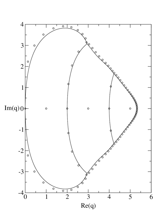
FIG. 2.: Locus ${\cal B}$ for the $m\to\infty$ limit of the family $B_{m}(6)$ with toroidal boundary conditions and chromatic zeros for $B_{m}(6)$ with $m=15$ (i.e., $n=90$).

The locus ${\cal B}$ has support for $Re(q)\geq 0$, and separates the $q$ plane into four regions. The outermost one, region $R_{1}$, extends to infinite $|q|$ and includes the intervals $q\geq q_{c}(B_{m}(6))$ and $q\leq 0$ on the real $q$ axis. Region $R_{2}$ includes the real interval $4\leq q\leq q_{c}(B_{m}(6))$, region $R_{3}$ includes the real interval $2\leq q\leq 4$, while region $R_{4}$ includes the real interval $0\leq q\leq 2$. In regions $R_{i}$, $1\leq i\leq 4$, the dominant terms are $\lambda_{B_{m}(6),0,1}$, $\lambda_{B_{m}(6),3,1}$, $\lambda_{B_{m}(6),2,1}$, and $\lambda_{B_{m}(6),1,1}$, respectively. Thus, the $q_{c}(B_{m}(6))$ given in (113) is the degeneracy between $|\lambda_{B_{m}(6),0,1}|$ and $|\lambda_{B_{m}(6),3,1}|$, and is the real solution of $q^{5}-19q^{4}+152q^{3}-660q^{2}+1600q-1761=0$.

III Family of Klein bottle Strips

Consider the graph with $L_{x}$ set of $K_{b}$ with $L_{x}-1$ edge linking sets $\{11,22,...,bb\}$ and one edge linking set $\{1b,2(b-1),...,b1\}$. This is the Klein bottle strip and will be denoted as ${\bar{B}}_{m}(b)$. The chromatic polynomials has the same form as given in eq. (6), and the $\lambda$’s are the same as those of the corresponding toroidal strip with the same $b$. The only difference is the coefficients.

A $L_{y}=5$ Klein bottle strip

For $b=5$ considered here, the coefficients $c_{{\bar{B}}_{m}(5),d,j}(q)c^{\prime}_{{\bar{B}}_{m}(5),d,j}$ are summarized in Table VIII

TABLE VIII.: Coefficients for $\bar{B}_{m}(5)$ strip.

$d$	$j$	partition	$c^{\prime}_{\bar{B}_{m}(5),d,j}$	$c_{\bar{B}_{m}(5),d,j}c^{\prime}_{\bar{B}_{m}(5),d,j}$
0	1	[0]	1	1
1	1	[1]	1	$q-1$
1	2	[1]	0	0
2	1	[2]	1	$\frac{1}{2}q(q-3)$
2	2	[2]	0	0
2	3	[2]	1	$\frac{1}{2}q(q-3)$
2	4	[11]	0	0
2	5	[11]	$-2$	$-(q-1)(q-2)$
3	1	[3]	1	$\frac{1}{6}q(q-1)(q-5)$
3	2	[3]	0	0
3	3	[3]	1	$\frac{1}{6}q(q-1)(q-5)$
3	4	[21]	0	0
3	5	[21]	2	$\frac{1}{3}q(q-2)(q-4)$
3	6	[21]	$-4$	$-\frac{2}{3}q(q-2)(q-4)$
3	7	[21]	2	$\frac{1}{3}q(q-2)(q-4)$
3	8	[111]	$-2$	$-\frac{1}{3}(q-1)(q-2)(q-3)$
3	9	[111]	0	0
4	1	[4]	1	$\frac{1}{24}q(q-1)(q-2)(q-7)$
4	2	[4]	0	0
4	3	[31]	0	0
4	4	[211]	0	0
4	5	[31]	$-6$	$-\frac{1}{6}q(q-1)(q^{2}-9q+17)$
		[22]	2
4	6	[31]	3	$\frac{1}{4}q(q-3)(q^{2}-7q+8)$
		[211]	3
4	7	[211]	$-6$	$-\frac{1}{6}q(q-5)(q^{2}-5q+7)$
		[22]	2
4	8	[1111]	0	0
4	9	[1111]	1	$\frac{1}{24}(q-1)(q-2)(q-3)(q-4)$
5	1	see text		$q-1$

where for $d=5$, it involves all possible partitions with appropriate $c^{\prime}_{\bar{B}_{m}(5),5,j}$ which are not listed here. Notice that the coefficients for $\lambda_{{\bar{B}}_{m}(5),d,j}$ with $(d,j)=(1,2)$, $(2,2)$, $(2,4)$, $(3,2)$, $(3,4)$, $(3,9)$, $(4,2)$, $(4,3)$, $(4,4)$, $(4,8)$ are zero, i.e., these ten $\lambda$’s do not contribute to the chromatic polynomial of the Klein bottle strip. We thus find that the total number of distinct $\lambda$’s for the $b=5$ Klein bottle strip with indicated linking is

$$N_{P,{\bar{B}}_{m}(5),\lambda}=17\ .$$ (114)

The sum of all of the coefficients for the Klein bottle strip is

$$C({\bar{B}}_{m}(5),q)=\sum_{d=0}^{5}\sum_{j=1}^{N_{{\bar{B}}_{m}(5),d,\lambda}}c_{{\bar{B}}_{m}(5),d,j}(q)c^{\prime}_{{\bar{B}}_{m}(5),d,j}=0\ ,$$ (115)

which is easy to understand by the coloring argument.

B $L_{y}=6$ Klein bottle strip

For $b=6$, the coefficients $c_{{\bar{B}}_{m}(6),d,j}(q)c^{\prime}_{{\bar{B}}_{m}(6),d,j}$ are summarized in Table IX

TABLE IX.: Coefficients for $\bar{B}_{m}(6)$ strip.

$d$	$j$	partition	$c^{\prime}_{\bar{B}_{m}(6),d,j}$	$c_{\bar{B}_{m}(6),d,j}c^{\prime}_{\bar{B}_{m}(6),d,j}$
0	1	[0]	1	1
1	1	[1]	1	$q-1$
1	2	[1]	$-1$	$-(q-1)$
2	1	[2]	1	$\frac{1}{2}q(q-3)$
2	2	[2]	$-1$	$-\frac{1}{2}q(q-3)$
2	3	[2]	3	$\frac{3}{2}q(q-3)$
2	4	[11]	$-1$	$-\frac{1}{2}(q-1)(q-2)$
2	5	[11]	$-2$	$-(q-1)(q-2)$
3	1	[3]	1	$\frac{1}{6}q(q-1)(q-5)$
3	2	[3]	$-1$	$-\frac{1}{6}q(q-1)(q-5)$
3	3	[3]	3	$\frac{1}{2}q(q-1)(q-5)$
3	4	[3]	$-3$	$-\frac{1}{2}q(q-1)(q-5)$
3	5	[21]	$-2$	$-\frac{1}{3}q(q-2)(q-4)$
3	6	[21]	6	$q(q-2)(q-4)$
3	7	[21]	$-4$	$-\frac{2}{3}q(q-2)(q-4)$
3	8	[21]	0	0
3	9	[111]	$-2$	$-\frac{1}{3}(q-1)(q-2)(q-3)$
3	10	[111]	2	$\frac{1}{3}(q-1)(q-2)(q-3)$
4	1	[4]	1	$\frac{1}{24}q(q-1)(q-2)(q-7)$
4	2	[4]	$-1$	$-\frac{1}{24}q(q-1)(q-2)(q-7)$
4	3	[4]	3	$\frac{1}{8}q(q-1)(q-2)(q-7)$
4	4	[31]	$-6$	$-\frac{1}{4}q(q-1)(q-3)(q-6)$
4	5	[31]	9	$\frac{3}{8}q(q-1)(q-3)(q-6)$
4	6	[31]	$-9$	$-\frac{3}{8}q(q-1)(q-3)(q-6)$
4	7	[31]	0	0
4	8	[31]	$-3$	$-\frac{1}{8}q(q-1)(q-3)(q-6)$
4	9	[22]	0	0
4	10	[22]	6	$\frac{1}{4}q(q-1)(q-4)(q-5)$
4	11	[22]	6	$-\frac{1}{2}q(q-5)$
		[211]	$-6$
4	12	[211]	6	$\frac{1}{4}q(q-2)(q-3)(q-5)$
4	13	[211]	0	0
4	14	[211]	$-9$	$-\frac{3}{8}q(q-2)(q-3)(q-5)$
4	15	[1111]	2	$\frac{1}{12}(q-1)(q-2)(q-3)(q-4)$
4	16	[1111]	1	$\frac{1}{24}(q-1)(q-2)(q-3)(q-4)$
5	1	[5]	1	$\frac{1}{120}q(q-1)(q-2)(q-3)(q-9)$
5	2	[5]	$-1$	$\frac{1}{60}q(q-1)(q-3)(7q^{2}-77q+216)$
		[221]	15
5	3	[41]	$-4$	$-\frac{1}{30}q(q-1)(q-2)(q-4)(q-8)$
5	4	[41]	12	$-q(q-2)(q-4)$
		[2111]	$-12$
5	5	[41]	$-8$	$-\frac{1}{15}q(q-1)(q-2)(q-4)(q-8)$
5	6	[32]	15	$\frac{1}{40}q(q-1)(q-7)(q^{2}-7q+2)$
		[311]	$-12$
5	7	[32]	$-15$	$-\frac{1}{60}(q-1)(q-2)(q-5)(7q^{2}-49q-6)$
		[11111]	1
5	8	[311]	12	$-\frac{1}{40}q(q-1)(q-3)(q^{2}-11q+38)$
		[221]	$-15$
5	9	[2111]	8	$\frac{1}{15}q(q-2)(q-3)(q-4)(q-6)$
5	10	[2111]	4	$\frac{1}{30}q(q-2)(q-3)(q-4)(q-6)$
5	11	[11111]	$-1$	$-\frac{1}{120}(q-1)(q-2)(q-3)(q-4)(q-5)$
6	1	see text		$-1$

where for $d=6$, it involves all possible partitions with appropriate $c^{\prime}_{\bar{B}_{m}(6),6,j}$ which are not listed here. Notice that the coefficients for $\lambda_{{\bar{B}}_{m}(6),d,j}$ with $(d,j)=(3,8)$, $(4,7)$, $(4,9)$, $(4,13)$ are zero, i.e., these four $\lambda$’s do not contribute to the chromatic polynomial of the Klein bottle strip. We thus find that the total number of distinct $\lambda$’s for the $b=6$ Klein bottle strip with indicated linking is

$$N_{P,{\bar{B}}_{m}(6)}=42\ .$$ (116)

The sum of all of the coefficients for the Klein bottle strip is again zero,

$$C({\bar{B}}_{m}(6),q)=\sum_{d=0}^{6}\sum_{j=1}^{N_{{\bar{B}}_{m}(6),d,\lambda}}c_{{\bar{B}}_{m}(6),d,j}(q)c^{\prime}_{{\bar{B}}_{m}(6),d,j}=0\ .$$ (117)

IV Properties of eigenvalues, coefficients, and ${\cal B}$

We first list the number of eigenvalues, $N_{B_{m}(b),d,\lambda}$, for $1\leq b\leq 6$, $0\leq d\leq b$, the total number of eigenvalues, $N_{P,B_{m}(b),\lambda}$, and the points at which ${\cal B}$ crosses the real $q$ axis, as well as the corresponding values for the Klein bottle strips in Table X.

TABLE X.: Properties of $P$ and ${\cal B}$ for strip graphs $B_{m}(b)$ and $\bar{B}_{m}(b)$. The properties apply for a given strip of size $L_{y}\times L_{x}$; some apply for arbitrary $L_{x}$, such as $N_{P,B_{m}(b),\lambda}$, while others apply for the infinite-length limit, such as the properties of the locus ${\cal B}$. For the boundary conditions in the $y$ and $x$ directions ($BC_{y}$, $BC_{x}$), P, and T denote periodic, and orientation-reversed (twisted) periodic. $N_{B_{m}(b),d,\lambda}$’s are abbreviated as $N_{d,\lambda}$, $N_{P,B_{m}(b),\lambda}$ is abbreviated as $N_{P,\lambda}$, and similarly for $\bar{B}_{m}(b)$ strips. The blank entries are zero. The column denoted BCR lists the points at which ${\cal B}$ crosses the real $q$ axis; the largest of these is $q_{c}(B_{m}(b))$ for the given family $B_{m}(b)$ or $\bar{B}_{m}(b)$. Column labelled “SN” refers to whether ${\cal B}$ has support for negative $Re(q)$, indicated as yes (y) or no (n).

$b$	$BC_{y}$	$BC_{x}$	$N_{0,\lambda}$	$N_{1,\lambda}$	$N_{2,\lambda}$	$N_{3,\lambda}$	$N_{4,\lambda}$	$N_{5,\lambda}$	$N_{6,\lambda}$	$N_{P,\lambda}$	BCR	SN
1	P	P	1	1						2	0, 2	n
2	P	P	1	2	1					4	0, 2	n
2	P	TP	1	2	1					4	0, 2	n
3	P	P	1	2	4	1				8	0, 2, 3	n
3	P	TP	1	1	2	1				5	0, 2, 3	n
4	P	P	1	2	5	7	1			16	0, 2, 3.67	n
4	P	TP	1	2	5	7	1			16	0, 2, 3.67	n
5	P	P	1	2	5	9	9	1		27	0, 2, 4, 4.51	n
5	P	TP	1	1	3	6	5	1		17	0, 2, 4, 4.51	n
6	P	P	1	2	5	10	16	11	1	46	0, 2, 4, 5.32	n
6	P	TP	1	2	5	9	13	11	1	42	0, 2, 4, 5.32	n

We conjecture the following $q$ value at which ${\cal B}$ crosses the real axis for the $B_{m}(b)$ strips,

$$\quad{\cal B}\supset\{q=0,\ 2,\ 4,...,2[\frac{b-1}{2}],q_{c}(B_{m}(b))\}\ .$$ (118)

where $[\nu]$ denotes the integral part of $\nu$, and the dominant eigenvalue in interval between $2(d^{\prime}-1)$ and $2d^{\prime}$ is $\lambda_{B_{m}(b),d^{\prime},1}$ for $1\leq d^{\prime}\leq[\frac{b+1}{2}]$.

The upper and lower bounds for the eigenvalues with coefficients of degree $b-1$ can be determined in the following theorem.

Theorem 1  The eigenvalues with coefficients of degree $b-1$ are bounded between $(-1)^{b-1}(q-1)$ and $(-1)^{b-1}(q-2b+1)$.

Proof.  Denote the $b!\times b!$ matrix for the eigenvalues with coefficients of degree $b-1$ as $M_{b-1}$. By theorem 2 of [58], the diagonal elements of $M_{b-1}$ are all the same to be $(-1)^{b-1}f_{b-1}(b,q)=(-1)^{b-1}(q-b)$, and other non-zero elements of $M_{b-1}$ are all the same to be $(-1)^{b}f_{b}(b,q)=(-1)^{b}$. Now consider $M^{\prime}_{b-1}=M_{b-1}-(-1)^{b-1}(q-b)I$, where $I$ is the $b!\times b!$ identity matrix. The number of non-zero elements, $(-1)^{b}$, in every row and columns of $M^{\prime}_{b-1}$ is $b-1$ by the construction of the matrix. If we denote the eigenvalues of $M^{\prime}_{b-1}$ as $\lambda^{\prime}$ and the normalized eigenvector of $M^{\prime}_{b-1}$ as $W^{T}=(w_{1},w_{2},...,w_{b!})$, then we have

$$M^{\prime}_{b-1}W=\lambda^{\prime}W$$ (119)

$$\Rightarrow |M^{\prime}_{b-1}W|^{2}=|\lambda^{\prime}W|^{2}$$ (121)

$$\Rightarrow (b-1)(w_{1}^{2}+w_{2}^{2}+...w_{b!}^{2})+2\sum_{i,j,i\neq j}w_{i}w_{j}=\lambda^{\prime 2}(w_{1}^{2}+w_{2}^{2}+...w_{b!}^{2})$$ (123)

$$\Rightarrow \lambda^{\prime 2}=b-1+2\sum_{i,j,i\neq j}w_{i}w_{j}\ ,$$ (125)

where we sum all the possible multiplications of two different $w_{i}$ and $w_{j}$ in each row of $M^{\prime}_{b-1}$. Therefore,

$$\lambda^{\prime 2} \leq b-1+\sum_{i,j,i\neq j}(w_{i}^{2}+w_{j}^{2})$$ (126)

$$= b-1+(b-1)(b-2)=(b-1)^{2}\ ,$$ (128)

that is, $-(b-1)\leq\lambda^{\prime}\leq b-1$. The upper and lower bounds for the eigenvalues of $M_{b-1}$ are

$$(-1)^{b-1}(q-b)\pm(b-1)=\cases{(-1)^{b-1}(q-1)&\cr(-1)^{b-1}(q-2b+1)&}\ .$$ (129)

It is easy to see that $(-1)^{b-1}(q-2b+1)$ is one of the principal terms and $(-1)^{b-1}(q-1)$ is one of the alternating terms given in [58]. It follows that these values are realized as the largest and smallest values for the eigenvalues of $M_{b-1}$  $\Box$.

We shall show that the locus ${\cal B}$ crosses the real $q$ axis at $q=0$, and doesn’t cross any $q\in{\mathbb{R}}_{\ -}$. We need the following lemma.

Lemma 1  On the non-positive real $q$ axis, the dominant eigenvalue with coefficient of degree $d$ is

$$\lambda_{B_{m}(b),d}=(-1)^{d}\sum_{j=0}^{d}(-1)^{j}{d\choose j}(b-d)^{(j)}f_{d+j}(b,q)\ .$$ (130)

Proof.  The matrix for the eigenvalues with coefficients of degree $d$ can be written as [58] $M_{d}=(-1)^{d}f_{d}(b,q)I+(-1)^{d+1}f_{d+1}(b,q)M_{d,1}+(-1)^{d+2}f_{d+2}(b,q)M_{d,2}+...$, where the non-zero elements are 1 in every $M_{d,j}$, and the number of these in each row and column is ${d\choose j}(b-d)^{(j)}$. By the same reason given in Theorem 1, the magnitudes of the eigenvalues of $M_{d,j}$ are bounded above by ${d\choose j}(b-d)^{(j)}$. Since the signs of $f_{d+j}(b,q)$ alternate for even $j$ and odd $j$ for any non-positive $q$ value, $\lambda_{B_{m}(b),d}$ given in eq. (130) is the upper bound for the eigenvalues with coefficients of degree $d$. Since $\lambda_{B_{m}(b),d}$ is the eigenvalue with $c^{\prime}_{B_{m}(b),d,j}=1$ given in [58], the proof is completed.  $\Box$.

Theorem 2  The minimum real $q$ at which ${\cal B}$ crosses the real $q$ axis is $q=0$.

Proof.  We will begin with the proof that $|\lambda_{B_{m}(b),0}|>|\lambda_{B_{m}(b),1}|>...$ on the whole negative real $q$ axis. The first few examples of $\lambda_{B_{m}(b),d}$’s are

$$\lambda_{B_{m}(b),0} = f_{0}(b,q)$$ (131)

$$\lambda_{B_{m}(b),1} = -f_{1}(b,q)+(b-1)f_{2}(b,q)$$ (133)

$$\lambda_{B_{m}(b),2} = f_{2}(b,q)-2(b-2)f_{3}(b,q)+(b-2)(b-3)f_{4}(b,q)$$ (135)

$$\lambda_{B_{m}(b),3} = -f_{3}(b,q)+3(b-3)f_{4}(b,q)-3(b-3)(b-4)f_{5}(b,q)+(b-3)(b-4)(b-5)f_{6}(b,q)$$ (137)

$$\lambda_{B_{m}(b),4} = f_{4}(b,q)-4(b-4)f_{5}(b,q)+6(b-4)(b-5)f_{6}(b,q)-4(b-4)(b-5)(b-6)f_{7}(b,q)$$ (141)

$$+(b-4)(b-5)(b-6)(b-7)f_{8}(b,q)\ .$$

To show that $f_{0}(b,q)$ has the largest magnitude on the negative real $q$ axis, we only need $|f_{i}(b,q)|>|f_{i+1}(b,q)-(b-i-1)f_{i+2}(b,q)|$ as follows,

$$|f_{i}(b,q)|-|f_{i+1}(b,q)-(b-i-1)f_{i+2}(b,q)|$$ (142)

$$= (-1)^{b-i}f_{i}(b,q)-(-1)^{b-i-1}\biggl{[}f_{i+1}(b,q)-(b-i-1)f_{i+2}(b,q)\biggr{]}$$ (144)

$$= (-1)^{b-i}\biggl{[}\sum_{s=0}^{b-i}(-1)^{s}{b-i\choose s}(q-i-s)^{(b-i-s)}+f_{i+1}(b,q)-(b-i-1)f_{i+2}(b,q)\biggr{]}$$ (146)

$$= (-1)^{b-i}\biggl{[}(q-i)^{(b-i)}+\sum_{s=0}^{b-i-1}(-1)^{s+1}{b-i\choose s+1}(q-i-s-1)^{(b-i-s-1)}$$ (150)

$$+\sum_{s=0}^{b-i-1}(-1)^{s}{b-i-1\choose s}(q-i-1-s)^{(b-i-1-s)}-(b-i-1)f_{i+2}(b,q)\biggr{]}$$

$$= (-1)^{b-i}\biggl{[}(q-i)^{(b-i)}+(-1)^{b-i}+(-1)^{b-i-1}+\sum_{s=0}^{b-i-2}(-1)^{s+1}(q-i-1-s)^{(b-i-1-s)}$$ (154)

$$\times\biggl{(}\frac{(b-i)!}{(s+1)!(b-i-s-1)!}-\frac{(b-i-1)!}{s!(b-i-1-s)!}\biggr{)}-(b-i-1)f_{i+2}(b,q)\biggr{]}$$

$$= (-1)^{b-i}\biggl{[}(q-i)^{(b-i)}+\sum_{s=0}^{b-i-2}(-1)^{s+1}(q-i-1-s)^{(b-i-1-s)}{b-i-1\choose s+1}$$ (158)

$$-(b-i-1)\sum_{s=0}^{b-i-2}(-1)^{s}{b-i-2\choose s}(q-i-2-s)^{(b-i-2-s)}\biggr{]}$$

$$= (-1)^{b-i}\biggl{[}(q-i)^{(b-i)}+\sum_{s=0}^{b-i-2}(-1)^{s+1}(q-i-2-s)^{(b-i-2-s)}$$ (162)

$$\times\biggl{[}(q-i-1-s)\frac{(b-i-1)!}{(s+1)!(b-i-2-s)!}+(b-i-1)\frac{(b-i-2)!}{s!(b-i-2-s)!}\biggr{]}\biggr{]}$$

$$= (-1)^{b-i}\biggl{[}(q-i)^{(b-i)}+\sum_{s=0}^{b-i-2}(-1)^{s+1}(q-i-2-s)^{(b-i-2-s)}(b-i-1){b-i-2\choose s}\frac{q-i}{s+1}\biggr{]}$$ (164)

$$> 0\quad{\rm for}\ q<0\ .$$ (166)

For $q=0$, all above argument are still valid, with the exception that $|f_{i}(b,0)|=|f_{i+1}(b,0)-(b-i-1)f_{i+2}(b,0)|$ when $i=0$, i.e. $|\lambda_{B_{m}(b),0}|=|\lambda_{B_{m}(b),1}|$ for $q=0$.  $\Box$.

We will prove that the maximal value of $q$ where ${\cal B}$ intersects the (positive) real axis is smaller than $q=b$ for $b\geq 2$. We have the following lemma.

Lemma 2  $f_{i}(b,q)\geq 0$ if $q\geq b$.

Proof.  Since we have $(q-i-s)^{(b-i-s)}>0$ when $q\geq b$, one only need to show that the magnitudes of the terms in eq. (8) decrease for $s$ from 0 to $b-i$.

$${b-i\choose s}(q-i-s)^{(b-i-s)}-{b-i\choose s+1}(q-i-s-1)^{(b-i-s-1)}$$ (167)

$$= (q-i-s-1)^{(b-i-s-1)}\biggl{[}\frac{(b-i)!}{s!(b-i-s)!}(q-i-s)-\frac{(b-i)!}{(s+1)!(b-i-s-1)!}\biggr{]}$$ (169)

$$= (q-i-s-1)^{(b-i-s-1)}\frac{(b-i)!}{(s+1)!(b-i-s)!}\biggl{[}(s+1)(q-i-s)-(b-i-s)\biggr{]}$$ (171)

$$= (q-i-s-1)^{(b-i-s-1)}\frac{(b-i)!}{(s+1)!(b-i-s)!}\biggl{[}s(q-i-s)+q-b\biggr{]}$$ (173)

$$\geq 0\quad{\rm for}\ 0\leq s\leq b-i-1\ {\rm and}\ q\geq b\ ,$$ (175)

where the equal sign is realized only when $s=0$ and $q=b$. Therefore, $f_{i}(b,q)=0$ only when $i=b-1$ at $q=b$, and $f_{i}(b,q)>0$ for any other $0\leq i\leq b$ and $q\geq b$.  $\Box$.

It is known that $q_{c}(B_{m}(1))=2$, $q_{c}(B_{m}(2))=2$ [9, 6], and $q_{c}(B_{m}(3))=3$ [10]. Thus, for $b=1$, $q_{c}=b+1$ while for $b=2$ and for $b=3$, $q_{c}$ has the respective values $q_{c}=b$. It is of interest to ask how $q_{c}(B_{m}(b))$ is related to $b$ for $b\geq 4$. We determine this relation with the following theorem.

Theorem 3  $q_{c}(B_{m}(b))<b$ for $b\geq 4$.

Proof.  By a reason similar to that given in Lemma 1 and the result of Lemma 2, the magnitude of the eigenvalues with coefficients of degree $d$ are bounded above by

$$\lambda^{\prime}_{B_{m}(b),d}=\sum_{j=0}^{d}{d\choose j}(b-d)^{(j)}f_{d+j}(b,q)\quad{\rm for}\ q\geq b\ ,$$ (176)

where it is equal to $\lambda_{B_{m}(b),b-1,1}$ for $d=b-1$ at $q=b$ and equal to $\lambda_{B_{m}(b),0,1}$ for $d=0$ and any $q$. The first few examples of $\lambda^{\prime}_{B_{m}(b),d}$’s are

$$\lambda^{\prime}_{B_{m}(b),0} = f_{0}(b,q)$$ (177)

$$\lambda^{\prime}_{B_{m}(b),1} = f_{1}(b,q)+(b-1)f_{2}(b,q)$$ (179)

$$\lambda^{\prime}_{B_{m}(b),2} = f_{2}(b,q)+2(b-2)f_{3}(b,q)+(b-2)(b-3)f_{4}(b,q)$$ (181)

$$\lambda^{\prime}_{B_{m}(b),3} = f_{3}(b,q)+3(b-3)f_{4}(b,q)+3(b-3)(b-4)f_{5}(b,q)+(b-3)(b-4)(b-5)f_{6}(b,q)$$ (183)

$$\lambda^{\prime}_{B_{m}(b),4} = f_{4}(b,q)+4(b-4)f_{5}(b,q)+6(b-4)(b-5)f_{6}(b,q)+4(b-4)(b-5)(b-6)f_{7}(b,q)$$ (187)

$$+(b-4)(b-5)(b-6)(b-7)f_{8}(b,q)\ .$$

To show that $f_{0}(b,q)=\lambda_{B_{m}(b),0,1}$ has the largest magnitude for $q\geq b$, we first need $f_{i}(b,q)>f_{i+1}(b,q)+(b-i-1)f_{i+2}(b,q)$ for $0\leq i\leq b-2$ and $q\geq b$,

$$f_{i}(b,q)-f_{i+1}(b,q)-(b-i-1)f_{i+2}(b,q)$$ (188)

$$= \sum_{s=0}^{b-i}(-1)^{s}{b-i\choose s}(q-i-s)^{(b-i-s)}-\sum_{s=0}^{b-i-1}(-1)^{s}{b-i-1\choose s}(q-i-1-s)^{(b-i-1-s)}$$ (192)

$$-(b-i-1)f_{i+2}(b,q)$$

$$= (-1)^{b-i}+\sum_{s=0}^{b-i-1}(-1)^{s}(q-i-1-s)^{(b-i-1-s)}\frac{(b-i-1)!}{s!(b-i-s)!}\biggl{[}(b-i)(q-i-s)-(b-i-s)\biggr{]}$$ (196)

$$-(b-i-1)f_{i+2}(b,q)$$

$$= (-1)^{b-i}+\sum_{s=0}^{b-i-1}(-1)^{s}(q-i-1-s)^{(b-i-1-s)}\biggl{[}{b-i-1\choose s}(b-i-1)+{b-i\choose s}(q-b)\biggr{]}$$ (200)

$$-(b-i-1)f_{i+2}(b,q)$$

$$= (-1)^{b-i}+(-1)^{b-i-1}[b-i-1+(b-i)(q-b)]+\sum_{s=0}^{b-i-2}(-1)^{s}(q-i-2-s)^{(b-i-2-s)}$$ (204)

$$\times\biggl{[}(q-i-1-s)\biggl{[}{b-i-1\choose s}(b-i-1)+{b-i\choose s}(q-b)\biggr{]}-(b-i-1){b-i-2\choose s}\biggr{]}$$

$$= (-1)^{b-i}+(-1)^{b-i-1}[b-i-1+(b-i)(q-b)]+\sum_{s=0}^{b-i-2}(-1)^{s}(q-i-2-s)^{(b-i-2-s)}$$ (210)

$$\times\biggl{[}(q-b)\biggl{[}{b-i-1\choose s}(b-i-1)+{b-i\choose s}(q-b)+(b-i-1-s){b-i\choose s}\biggr{]}$$

$$+(b-i-1)(b-i-2){b-i-2\choose s}\biggr{]}$$

$$\geq 0\quad{\rm for}\ 0\leq i\leq b-2\ {\rm and}\ q\geq b\ ,$$ (212)

where the equal sign is realized only when $i=b-2$ at $q=b$. Therefore, we have $\lambda^{\prime}_{B_{m}(b),0}>\lambda^{\prime}_{B_{m}(b),1}>...>\lambda^{\prime}_{B_{m}(b),b/2}$ for even $b$ and $\lambda^{\prime}_{B_{m}(b),0}>\lambda^{\prime}_{B_{m}(b),1}>...>\lambda^{\prime}_{B_{m}(b),(b-1)/2}$ for odd $b$. Recall $f_{i}(b,q)=0$ if $b<i$. To show $\lambda^{\prime}_{B_{m}(b),b/2}>...>\lambda^{\prime}_{B_{m}(b),b}$ for even $b$ and $\lambda^{\prime}_{B_{m}(b),(b+1)/2}>...>\lambda^{\prime}_{B_{m}(b),b}$ for odd $b$, we must have the coefficient of $f_{b}(b,q)$ in $\lambda^{\prime}_{B_{m}(b),d}$ is smaller than the sum of the coefficients of $f_{b-2}(b,q)$ and $f_{b}(b,q)$ in $\lambda^{\prime}_{B_{m}(b),d-1}$ as follows,

$${d-1\choose b-d-1}(b-d+1)^{(b-d-1)}+{d-1\choose b-d+1}(b-d+1)^{(b-d+1)}-{d\choose b-d}(b-d)^{(b-d)}$$ (213)

$$= \frac{(d-1)!(b-d+1)!}{(b-d-1)!(2d-b)!2}+\frac{(d-1)!(b-d+1)!}{(b-d+1)!(2d-b-2)!}-\frac{d!(b-d)!}{(b-d)!(2d-b)!}$$ (215)

$$= \frac{(d-1)!}{(2d-b)!}\frac{(b-d+1)(b-d)}{2}+\frac{(d-1)!}{(2d-b-2)!}-\frac{d!}{(2d-b)!}$$ (217)

$$= \frac{(d-1)!}{2(2d-b)!}\biggl{[}(b-d+1)(b-d)+2(2d-b)(2d-b-1)-2d\biggr{]}$$ (219)

$$= \frac{(d-1)!}{2(2d-b)!}(3b^{2}-10bd+9d^{2}+3b-7d)\ ,$$ (221)

which is larger than 0 for even $b$ with $b/2<d\leq b$ and odd $b$ with $(b+1)/2<d\leq b$ except for $(b,d)=(2,2)$ and $(4,3)$ where it is 0. For odd $b$ and $d=(b+1)/2$, there is no $f_{b}(b,q)$ term in $\lambda^{\prime}_{B_{m}(b),(b-1)/2}$, and we need the coefficient of the $f_{b}(b,q)$ in $\lambda^{\prime}_{B_{m}(b),(b+1)/2}$ is smaller than the coefficient of $f_{b-2}(b,q)$ in $\lambda^{\prime}_{B_{m}(b),(b-1)/2}$,

$${d-1\choose b-d-1}(b-d+1)^{(b-d-1)}-{d\choose b-d}(b-d)^{(b-d)}$$ (222)

$$= \frac{(d-1)!(b-d+1)!}{2(b-d-1)!(2d-b)!}-\frac{d!(b-d)!}{(b-d)!(2d-b)!}$$ (224)

$$= \frac{(d-1)!}{2(2d-b)!}\biggl{[}(b-d+1)(b-d)-2d\biggr{]}$$ (226)

$$= \frac{1}{2}(\frac{b-1}{2})!\biggl{[}(\frac{b+1}{2})(\frac{b-1}{2})-(b+1)\biggr{]}$$ (228)

$$= \frac{1}{8}(\frac{b-1}{2})!(b-5)(b+1)\geq 0\quad{\rm for}\ b\geq 5\ .$$ (230)

Therefore, for $b\geq 4$, we find $\lambda_{B_{m}(b),0,1}$ is dominant for $q\geq b$, i.e. $q_{c}(B_{m}(b))<b$.  $\Box$.

We remark that our theorem, in combination with the known results that $q_{c}(B_{m}(b))=b$ for $b=2,3$, yields the theorem that

$$q_{c}(B_{m}(b))\leq b\quad{\rm for}\quad b\geq 2\ .$$ (231)

We observe that the length between $b$ and $q_{c}(B_{m}(b))$ are $-1,0,0,0.3264,0.4937$, and 0.6764 for the respective values $1\leq b\leq 6$. These values suggest that this length might well increase monotonically up to 1 as $b\to\infty$, since the lower bound for $q_{c}(B_{m}(b))$ is $b-1$ [62].

We observe the following general form of four $\lambda_{B_{m}(b),3,j}$ corresponding to the partition $[21]$,

$$\lambda_{B_{m}(b),3,j_{1}}=-f_{3}(b,q)+2(b-3)f_{4}(b,q)-(b-3)(b-4)f_{5}(b,q)$$ (232)

$$\lambda_{B_{m}(b),3,j_{2}}=-f_{3}(b,q)+(b-4)f_{4}(b,q)+(b-4)f_{5}(b,q)$$ (233)

$$\lambda_{B_{m}(b),3,j_{3}}=-f_{3}(b,q)+(b-6)f_{4}(b,q)+3(b-4)f_{5}(b,q)$$ (234)

$$\lambda_{B_{m}(b),3,j_{4}}=-f_{3}(b,q)-3f_{4}(b,q)-3f_{5}(b,q)\ .$$ (235)

These formulae are correct for $3\leq b\leq 9$, and we conjecture that these are the only $\lambda_{B_{m}(b),3,j}$ corresponding to the partition $[21]$ for arbitrarily $b$. For toroidal strips, their coefficients are $c_{B_{m}(b),3,j}=\frac{1}{6}q(q-2)(q-4)$, and $c^{\prime}_{B_{m}(b),3,j_{k}}=2(b-1),b(b-3),(b-1)(b-2)$, and $\frac{2}{3}b(b-2)(b-4)$ for $1\leq k\leq 4$.

From toroidal strips to Klein bottle strips, we observe the transformations from $c^{\prime}_{{B}_{m}(b),d,j}$ to $c^{\prime}_{{\bar{B}}_{m}(b),d,j}$ have certain patterns for $0\leq d\leq 4$ and $2\leq b\leq 6$, and summarized them in table XI. Notice that the results are different for even and odd $b$.

TABLE XI.: Relation of $c^{\prime}_{{B}_{m}(b),d,j}$ and $c^{\prime}_{{\bar{B}}_{m}(b),d,j}$

partition	$d$	$c^{\prime}_{{B}_{m}(b),d,j}$	$c^{\prime}_{{\bar{B}}_{m}(b),d,j}$ for odd $b$	$c^{\prime}_{{\bar{B}}_{m}(b),d,j}$ for even $b$
$[d]$	$d\geq 0$	1	1	1
	$d\geq 1$	$b-1$	0	$-1$
	$d\geq 2$	$b(b-3)/2$	$(b-3)/2$	$b/2$
	$d\geq 3$	$b(b-1)(b-5)/6$	0	$-b/2$
	$d\geq 4$	$b(b-1)(b-2)(b-7)/24$	$(b-1)(b-7)/8$	$b(b-2)/8$
$[1^{d}]$	2	$b-1$	0	$-1$
	2,3	$(b-1)(b-2)/2$	$-(b-1)/2$	$-(b-2)/2$
	3,4	$(b-1)(b-2)(b-3)/6$	0	$(b-2)/2$
	4,5	$(b-1)(b-2)(b-3)(b-4)/24$	$(b-1)(b-3)/8$	$(b-2)(b-4)/8$
$[21]$	3	$2(b-1)$	0	$-2$
	3	$b(b-3)$	$b-3$	$b$
	3	$(b-1)(b-2)$	$-(b-1)$	$-(b-2)$
	3	$2b(b-2)(b-4)/3$	2	0
$[31]$	4	$3(b-1)$	0	$-3$
	4	$3b(b-3)/2$	$3(b-3)/2$	$3b/2$
	4	$3(b-1)(b-2)/2$	$-3(b-1)/2$	$-3(b-2)/2$
	4	$b(b-1)(b-5)/2$	0	$-3b/2$
	4	$b(b-2)(b-4)$	3	0
	4	$3b(b-1)(b-3)(b-6)/8$	$-3(b-1)(b-3)/8$	$-3b(b-6)/8$
$[22]$	4	$b(b-3)$	$b-3$	$b$
	4	$2b(b-2)(b-4)/3$	2	0
	4	$b(b-1)(b-4)(b-5)/6$	$(b-1)(b-5)/2$	$b(b-4)/2$
$[211]$	4	$3(b-1)(b-2)/2$	$-3(b-1)/2$	$-3(b-2)/2$
	4	$(b-1)(b-2)(b-3)/2$	0	$3(b-2)/2$
	4	$b(b-2)(b-4)$	3	0
	4	$3b(b-2)(b-3)(b-5)/8$	$-3(b-3)(b-5)/8$	$-3b(b-2)/8$

For the partition $[d]$, if we label $c^{\prime}_{{B}_{m}(b),d\geq 0}$ as the $c^{\prime}_{{B}_{m}(b),d,j}=1$ in the first row of table XI, and similarly for other $c^{\prime}_{{B}_{m}(b),d\geq d^{\prime}}$, we conjecture the following forms of the corresponding $c^{\prime}_{{\bar{B}}_{m}(b),d\geq d^{\prime}}$ for general $d^{\prime}$,

$$c^{\prime}_{{\bar{B}}_{m}(b),d\geq d^{\prime}}=\cases{{(b-1)/2\choose d^{\prime}/2}-{(b-1)/2\choose d^{\prime}/2-1}&for even $d^{\prime}\geq 2$\cr 0&for odd $d^{\prime}\geq 1$}\quad{\rm for\ odd\ }b\ ,$$ (236)

and

$$c^{\prime}_{{\bar{B}}_{m}(b),d\geq d^{\prime}}=\cases{{b/2\choose d^{\prime}/2}&for even $d^{\prime}\geq 0$\cr-{b/2\choose(d^{\prime}-1)/2}&for odd $d^{\prime}\geq 1$}\quad{\rm for\ even\ }b\ .$$ (237)

For the partition $[1^{d}]$, if we label $c^{\prime}_{{B}_{m}(b),2}$ as the $c^{\prime}_{{B}_{m}(b),d,j}=b-1$ in the first row of the $[1^{d}]$ partition of table XI, and similarly for other $c^{\prime}_{{B}_{m}(b),d^{\prime}}$, we conjecture the following forms of the corresponding $c^{\prime}_{{\bar{B}}_{m}(b),d^{\prime}}$ for general $d^{\prime}$,

$$c^{\prime}_{{\bar{B}}_{m}(b),d^{\prime}}=\cases{(-1)^{(d^{\prime}-1)/2}{(b-1)/2\choose(d^{\prime}-1)/2}&for odd $d^{\prime}\geq 3$\cr 0&for even $d^{\prime}\geq 2$}\quad{\rm for\ odd\ }b\ ,$$ (238)

and

$$c^{\prime}_{{\bar{B}}_{m}(b),d^{\prime}}=\cases{\sum^{(d^{\prime}-1)/2}_{j=0}(-1)^{j}{b/2\choose j}&for odd $d^{\prime}\geq 3$\cr\sum^{(d^{\prime}-2)/2}_{j=0}(-1)^{j-1}{b/2\choose j}&for even $d^{\prime}\geq 2$}\quad{\rm for\ even\ }b\ ,$$ (239)

If the sum of the coefficients for a specific $d$ is denoted as $C({\bar{B}}_{m}(b),d,q)$, that is,

$$C({\bar{B}}_{m}(b),d,q)=\sum_{j=1}^{N_{{\bar{B}}_{m}(b),d,\lambda}}c_{{\bar{B}}_{m}(b),d,j}(q)c^{\prime}_{{\bar{B}}_{m}(b),d,j}\ ,$$ (240)

we have the following conjecture,

$$C({\bar{B}}_{m}({\rm even}\ b),d,q)=\cases{(-1)^{d/2}{b/2\choose d/2}&for even $d$\cr 0&for odd $d$}$$ (241)

$$C({\bar{B}}_{m}({\rm odd}\ b),d,q)=\cases{(-1)^{d/2}{(b-1)/2\choose d/2}&for even $d$\cr(-1)^{(d-1)/2}(q-1){(b-1)/2\choose(d-1)/2}&for odd $d$}\ .$$ (242)

V Conclusions

In this paper we have presented exact zero-temperature partition functions for families of chain graphs composed of repeated complete subgraphs $K_{b}$, $b=5,6$ with periodic or twisted periodic boundary condition in the longitudinal direction. In the $L_{x}\to\infty$ limit, the continuous accumulation set of chromatic zeros ${\cal B}$ was determined. We showed the eigenvalues with coefficients of degree $b-1$ are bounded between $(-1)^{b-1}(q-1)$ and $(-1)^{b-1}(q-2b+1)$, and gave the explicit forms of the eigenvalues for partitions of the form [21]. The minimum real $q$ at which ${\cal B}$ crosses the real $q$ axis was proven to be $q=0$, and $q_{c}(B_{m}(b))<b$ for $4\leq b$.

Acknowledgment: I would like to thank Prof. R. Shrock for helpful discussions.

REFERENCES

[1]R. B. Potts, Proc. Camb. Phil. Soc. 48 (1952) 106.
[2]F. Y. Wu, Rev. Mod. Phys. 54 (1982) 235.
[3]R. C. Read, J. Combin. Theory 4 (1968) 52.
[4]R. C. Read and W. T. Tutte, “Chromatic Polynomials”, in
Selected Topics in Graph Theory, 3, eds. L. W. Beineke and R. J.
Wilson (Academic Press, New York, 1988.).
[5]N. L. Biggs, Algebraic Graph Theory (2nd ed.,
Cambridge Univ. Press, Cambridge, 1993).
[6]R. Shrock and S.-H. Tsai, Phys. Rev. E55 (1997) 5165.
[7]N. L. Biggs, LSE report LSE-CDAM-99-08 (1999).
[8]S. Beraha, J. Kahane, and N. Weiss, J. Combin. Theory B
27 (1979) 1; ibid., 28 (1980) 52.
[9]N. L. Biggs, R. M. Damerell, and D. A. Sands, J. Combin. Theory
B 12 (1972) 123.
[10]N. L. Biggs and R. Shrock, J. Phys. A (Letts) 32, L489
(1999).
[11]S.-C. Chang, Physica A296, 495 (2001).
[12]E. H. Lieb, Phys. Rev. 162 (1967) 162.
[13]S.-C. Chang and R. Shrock, Phys. Rev. E, 62, 4650
(2000).
[14]S.-C. Chang and R. Shrock, Physica A 296 (2001) 131.
[15]N. L. Biggs and G. H. Meredith, J. Combin. Theory B20
(1976) 5.
[16]N. L. Biggs and G. H. Meredith, J. Combin. Theory B20
(1976) 5.
[17]N. L. Biggs, Bull. London Math. Soc. 9 (1977) 54.
[18]R. C. Read, in Proc. 3rd Caribbean Conf. on Combin. and
Computing (1981).
[19]R. C. Read, in Proc. 5th Caribbean Conf. on Combin. and
Computing (1988).
[20]R. J. Baxter, J. Phys. A 20 (1987) 5241.
[21]R. C. Read and G. F. Royle, in Graph Theory,
Combinatorics, and Applications (Wiley, NY, 1991), vol. 2, p. 1009.
[22]R. Shrock and S.-H. Tsai, Phys. Rev. E55 (1997) 6791.
[37]N. L. Biggs, J. Combin. Theory B 82, 19 (2001);
Bull. London Math. Soc., in press.
[38]R. Shrock, in the Proceedings of the 1999 British
Combinatorial Conference, BCC99, Discrete Math. 231 (2001) 421.
[39]H. Kluepfel and R. Shrock, unpublished; H. Kluepfel, Stony Brook
thesis “The -State Potts Model: Partition Functions and Their Zeros in the
Complex Temperature and Planes” (July, 1999).
[40]R. Shrock, Physica A281, 221 (2000).
[41]S.-C. Chang and R. Shrock, Phys. Rev. E62, 4650 (2000).
[42]R. Shrock, Physica A283, 388 (2000).
[43]S.-C. Chang and R. Shrock, Physica A286, 189 (2000).
[44]S.-C. Chang and R. Shrock, Physica A 290, 402 (2001).
[45]S.-C. Chang and R. Shrock, Ann. Phys. 290, 124 (2001).
[46]S.-C. Chang and R. Shrock, Phys. Rev. E62, 4650 (2000).
[47]J. Salas and A. Sokal, J. Stat. Phys., 104, 611 (2001).
[48]S.-C. Chang and R. Shrock, Physica A 286, 189 (2000).
[49]S.-C. Chang and R. Shrock, Physica A 292, 307 (2001).
[50]S.-C. Chang and R. Shrock, Physica A 296, 234
(2001).
[51]S.-C. Chang and R. Shrock, Physica A 296, 183 (2001).
[52]S.-C. Chang and R. Shrock, Int. J. Mod. Phys. B 15,
443 (2001).
[53]J. L. Jacobsen and J. Salas, J. Stat. Phys. 104, 703
(2001).
[54]J. Salas and R. Shrock, Phys. Rev. E 64, 011111 (2001).
[55]S.-C. Chang and R. Shrock, Physica A, 301, 301 (2001).
[56]S.-C. Chang and R. Shrock, Phys. Rev. E, in
press; cond-mat/0107012.
[57]J. Salas, S.-C. Chang and R. Shrock, J. Stat. Phys., in press
(cond-mat/0108144).
[58]N. L. Biggs, “Chromatic polynomials and representations
of the symmetric group”, AGT workshop, Edinburgh (July 2001), LSE
report LSE-CDAM-01-02 (2001).
[59]N. L. Biggs, M. Klin, and P. Reinfeld, “Algebraic methods
for chromatic polynomials”, AGT workshop, Edinburgh (July, 2001), LSE
report LSE-CDAM-01-06 (2001).
[60]N. L. Biggs, LSE report LSE-CDAM-00-04 (May 2000).
[61]N. L. Biggs and P. Reinfeld, LSE report LSE-CDAM-00-07
(June 2000),
http://www.cdam.lse.ac.uk/Reports/ .
[62]N. L. Biggs, S.-C. Chang, P. Reinfeld, and R. Shrock, in
preparation.