The monodromy of the Lagrange top and the Picard-Lefschetz formula

Abstract

The purpose of this paper is to show that the monodromy of action variables of the Lagrange top and its generalizations can be deduced from the monodromy of cycles on a suitable hyperelliptic curve (computed by the Picard-Lefschetz formula).

1 Introduction

Let $(M,\omega)$ be a symplectic manifold of dimension $2n$ and consider a Lagrangian fibration

$$\begin{array}[]{cccl}F:&M&\longrightarrow&B\\ \end{array}.$$

where $B$ is a manifold of dimension $n$. We shall also suppose that each fiber $F_{q}=F^{-1}(q)$ is compact and connected, so it is diffeomorphic to a Liouville torus.

For each $q\in B$ there is an open neighborhood $U\subset B$ of $q$ and a diffeomorphism

$$V=F^{-1}(U)\longrightarrow U\times{\bf T}^{n}:p\longmapsto(I_{1},...,I_{n},\phi_{1},...,\phi_{n})$$

where ${\bf T}^{n}$ is the $n$-torus $\mathbb{R}^{n}/\mathbb{Z}^{n}$. Moreover the coordinates $I_{i}$, called action coordinates, are smooth functions depending on $q$ only, and in these coordinates the symplectic form is

$$\omega=\sum_{i=1}^{n}d\phi_{i}\wedge dI_{i}.$$

The coordinates $\phi_{i}$ are called angle coordinates. Thus $V$ has the structure of a symplectic principal bundle with a structure group ${\bf T}^{n}$, Lagrangian fibers, and a Hamiltonian action of the structure group whose momentum map is the projection map of the bundle.

The question of global existence of action-angle coordinates on the principal bundle $M\longrightarrow B$ has been studied in a pioneering paper by Duistermaat [12]. A most obvious obstruction to the global existence of such coordinates is of course the monodromy of the bundle, which is a homomorphism from $\pi_{1}(B,b)$ to $H_{1}(F_{b},\mathbb{Z})=\mathbb{Z}^{n}$. The first example of a mechanical system with non-trivial monodromy is due to R. Cushman (the spherical pendulum, see [12]). It turned out later that many other integrable systems have this property. We mention here the Lagrange top [10], the spherical pendulum with quadratic potential $(x_{3}-a)^{2}$ [40], the so called Kirchoff top (a rigid body in an infinite ideal fluid) [6].

General theorems in this direction are due to M. Zou [39] and T.Z. Nguyen [26]. These results have an analytical nature: they do not use the underlying algebro-geometric structure of the problem. In the present paper we shall develop this second (algebro-geometric) approach on a concrete example: the Lagrange top and its generalizations. The idea of the proof is the following. Let us suppose that we have an algebraically completely integrable Hamiltonian system. This defines a Lagrangian fibration and we suppose that each Lagrangian fiber (Liouville torus) can be complexified to an affine part of a Jacobian variety $J(\Gamma_{b})=H^{0}(\Gamma_{b},\Omega^{1})^{*}/H_{1}(\Gamma_{b},\mathbb{Z})$, where $\Gamma_{b}$ is a spectral curve depending on $b$. The manifold $B$ is the complement to the discriminant locus of the spectral curve $\Gamma_{b}$. It is easier to describe the monodromy of the complexified Lagrangian fibration (with fibers $J(\Gamma_{b})$). Indeed, its monodromy coincides with the monodromy of the homology Milnor bundle with fibers $H_{1}(\Gamma_{b},\mathbb{Z})$ and base $B$. We recall that the latter is associated to the Milnor fibration of the polynomial defining the spectral curve $\Gamma_{b}$. In particular it comes with a canonical Gauss-Manin connection and its monodromy is computed by the Picard-Lefschetz theory (e.g.[4]). Once the monodromy of the cycles of the homology Milnor bundle computed, it remains to consider the monodromy of the cycles generating the homology of the real part of $J(\Gamma_{b})$, and hence of the real Liouville tori.

Of course if $B$ is simply connected there is no (real !) monodromy at all. A simplified, but sufficiently general example is when $\Gamma_{b}$ is defined by a polynomial which itself is a versal deformation of an isolated real simple singularity. The complement to the real part of the complex discriminant locus may be not simply connected (this set should not be confused with the complement to the real discriminant locus, see [22]). The simplest non-trivial example is the $A_{3}$ singularity $y^{2}\pm x^{4}$ and the curve defined by its real versal deformation is related to the spectral curve of the spherical pendulum [18]. Indeed, the discriminant locus $\Delta_{ab}$ of the polynomial $(x^{2}+1)^{2}+ax+b$ contains an isolated point ($a=0,b=0$).

The paper is organized as follows. In section 2 we define the generalized Lagrange top as a $g+1$ degrees of freedom completely integrable Hamiltonian system. The underlying algebro-geometric structure is explained in section 3. It turns out that, by analogy to the classical Lagrange top ($g=1$) [16], each complexified Liouville torus is an affine part of a generalized Jacobian $J(\Gamma^{\prime})=H^{0}(\Gamma,\Omega^{1}(\infty^{+}+\infty^{-})^{*}/H_{1}(\Gamma_{aff},\mathbb{Z})$ of a genus $g$ hyperelliptic curve $\Gamma$. Here $\Gamma_{aff}$ is a smooth compact affine curve, $\Gamma$ is the compactified and normalized $\Gamma_{aff}$, $X\backslash\Gamma_{aff}=\infty^{+}+\infty^{-}$, $\Gamma^{\prime}$ is a compact singular curve obtained from $\Gamma$ by identifying $\infty^{+}$ and $\infty^{-}$. Therefore to compute the monodromy of Liouville tori we have to determine first the monodromy of the homology bundle of $\Gamma_{aff}$ (on the place of $\Gamma$), and then the monodromy of the cycles of $H_{1}(\Gamma_{aff},\mathbb{Z})$ which generate the homology of the real part of $J(\Gamma^{\prime})$. For this reason we need the real structure of $J(\Gamma^{\prime})$ which is described in section 4. Finally, using this and the Picard-Lefschetz formula, we compute the monodromy of the top, provided that $g\leq 2$ (section 5).

This paper is an extended version of [35]. I would like to thank Lubomir Gavrilov who suggested me the idea of the paper.

2 Definition of the generalized Lagrange top

Consider the following Lax pair

$$\frac{d}{dt}\Gamma(\lambda)=\left[\Gamma(\lambda),\chi\lambda+\Omega\right].$$ (1)

where

$$\Gamma(\lambda)=\chi\lambda+\Gamma_{0}-\Gamma_{1}\lambda^{-1}\cdots-\Gamma_{g}\lambda^{-g}\in\mathfrak{so}(3)[\lambda,\lambda^{-1}],g\in\mathbb{N},$$

$$\chi=\left(\begin{array}[]{ccc}0&-1&0\\ 1&0&0\\ 0&0&0\\ \end{array}\right),\quad\Omega=\left(\begin{array}[]{ccc}0&-\omega_{3}&\omega_{2}\\ \omega_{3}&0&-\omega_{1}\\ -\omega_{2}&\omega_{1}&0\\ \end{array}\right),$$

$$\Gamma_{0}=\left(\begin{array}[]{ccc}0&-(1+m)\omega_{3}&\omega_{2}\\ (1+m)\omega_{3}&0&-\omega_{1}\\ -\omega_{2}&\omega_{1}&0\\ \end{array}\right),\quad i\in\{1,2,...,g\}\quad\Gamma_{i}=\left(\begin{array}[]{ccc}0&-\gamma_{i,3}&\gamma_{i,2}\\ \gamma_{i,3}&0&-\gamma_{i,1}\\ -\gamma_{i,2}&\gamma_{i,1}&0\\ \end{array}\right).$$

To simplify the notations we note below

$$\gamma_{0,1}=\omega_{1},\quad\gamma_{0,2}=\omega_{2},\quad\gamma_{0,3}=(1+m)\omega_{3}.$$

The Lax pair (1) has $2g+2$ first integrals

$$H_{k}=-\frac{1}{4}\mbox{residue}_{\lambda=0}(\lambda^{k-1}tr(\Gamma(\lambda)^{2})),k=-1,0,1,...,2g.$$

We have in particular

$$H_{-1}=(1+m)\omega_{3},\quad H_{0}=\frac{1}{2}\left(\omega_{1}^{2}+\omega_{2}^{2}+(1+m)^{2}\omega_{3}^{2}\right)-\gamma_{1,3}.$$

The Lax pair (1) can be written in an equivalent form as a Hamiltonian system

$$\frac{d}{dt}x=\{x,H\},$$

where

$$H=H_{0}-\frac{m}{2(1+m)}H_{-1}^{2}=\frac{1}{2}\left(\omega_{1}^{2}+\omega_{2}^{2}+(1+m)\omega_{3}^{2}\right)-\gamma_{1,3}.$$

The Poisson structure $\{.,.\}$ is given by

$$\{\gamma_{i,k},\gamma_{j,l}\}=\sum_{c=1}^{3}\Lambda_{kl}^{c}\gamma_{{i+j},c}\quad\mbox{for }i,j\in\{0,1,...,g\}.$$ (2)

where $\Lambda_{kl}^{c}$ is a skew-symmetric matrix

$$\Lambda_{12}=\left(\Lambda_{12}^{1},\Lambda_{12}^{2},\Lambda_{12}^{3}\right)=(0,0,-1),\quad\Lambda_{13}=\left(\Lambda_{13}^{1},\Lambda_{13}^{2},\Lambda_{13}^{3}\right)=(0,1,0),\quad\Lambda_{23}=\left(\Lambda_{23}^{1},\Lambda_{23}^{2},\Lambda_{23}^{3}\right)=(-1,0,0).$$

It is easy to check further that (1) is a Liouville completely integrable Hamiltonian system of $g+1$ degrees of freedom, where $H_{i}$, $i=-1,0,...,g-1$ are first integrals, while $H_{j}$, $j=g,g+1,...,H_{2g}$ are Casimirs.

We call the system (1) the generalized Lagrange top (another generalization may be found in [29]).

We shall identify the Lie algebras $(\mathfrak{so}(3),[.,.])$ and $(\mathbb{R}^{3},\wedge)$ by the Lie algebras anti-isomorphism ($[A,B]=-A\wedge B)$

$$\left(\begin{array}[]{ccc}0&-x_{3}&x_{2}\\ x_{3}&0&-x_{1}\\ -x_{2}&x_{1}&0\\ \end{array}\right)\in\mathfrak{so}(3)\longmapsto(x_{3},x_{2},x_{1})\in\mathbb{R}^{3}.$$

Let $\sigma_{1},\sigma_{2},\sigma_{3}$ be the Pauli spin matrices, defined by

$$\sigma_{1}=\left(\begin{array}[]{cc}1&0\\ 0&-1\end{array}\right),\quad\sigma_{2}=\sqrt{-1}\left(\begin{array}[]{cc}0&-1\\ 1&0\end{array}\right),\quad\sigma_{3}=\left(\begin{array}[]{cc}0&1\\ 1&0\end{array}\right),$$

and denote $\sigma=(\sigma_{1},\sigma_{2},\sigma_{3}).$ Then $[\sigma_{1},\sigma_{2}]=2\sqrt{-1}\sigma_{3}$ (+cyclic permutation) which implies that the map

$$x=\left(x_{3},x_{2},x_{1}\right)\in\mathbb{R}^{3}\longmapsto\frac{1}{2\sqrt{-1}}\widetilde{x}=\frac{1}{2\sqrt{-1}}x.\sigma=\frac{1}{2}\left(\begin{array}[]{cc}-\sqrt{-1}x_{1}&-\sqrt{-1}x_{3}-x_{2}\\ -\sqrt{-1}x_{3}+x_{2}&\sqrt{-1}x_{1}\end{array}\right)\in\mathfrak{su}(2),$$

where $\widetilde{x}=x.\sigma=x_{1}\sigma_{1}+x_{2}\sigma_{2}+x_{3}\sigma_{3}$ is a Lie algebra isomorphism between $\mathbb{R}^{3}$ and the $(2\times 2)$ skew-Hermitian traceless matrices $\mathfrak{su}(2)$. Note that

$$-\det(x.\sigma)=||x||^{2},\quad\mbox{and trace}(\widetilde{x}\widetilde{y})=-\frac{1}{2}x.y.$$

Composing these two previous morphisms of Lie algebras we get a Lie algebras anti-isomorphism between $(\mathfrak{so}(3),[.,.])$ and $(\mathfrak{su}(2),[.,.])$, we deduce from (1) an equivalent Lax pair. Namely,

$$\mathfrak{so}(3)\ni\chi\longmapsto\frac{1}{2\sqrt{-1}}\sigma_{3}\in\mathfrak{su}(2),$$

$$\mathfrak{so}(3)\ni\Omega\longmapsto\frac{1}{2\sqrt{-1}}\widetilde{\Omega}=\frac{1}{2\sqrt{-1}}\left(\begin{array}[]{cc}\omega_{1}&\omega_{3}-\sqrt{-1}\omega_{2}\\ \omega_{3}+\sqrt{-1}\omega_{2}&-\omega_{1}\end{array}\right)\in\mathfrak{su}(2),$$

and finally

$$\mathfrak{so}(3)\ni\Gamma_{i}\longmapsto\frac{1}{2\sqrt{-1}}\widetilde{\Gamma}_{i}=\frac{1}{2\sqrt{-1}}\left(\begin{array}[]{cc}\gamma_{i,1}&\gamma_{i,3}-\sqrt{-1}\gamma_{i,2}\\ \gamma_{i,3}+\sqrt{-1}\gamma_{i,2}&-\gamma_{i,1}\end{array}\right)\in\mathfrak{su}(2),i=1,2,...,g.$$

If we denote

$$U(x)=x^{g+1}+\left((1+m)\omega_{3}-\sqrt{-1}\omega_{2}\right)x^{g}-\left(\gamma_{1,3}-\sqrt{-1}\gamma_{1,2}\right)x^{g-1}-\cdots-(\gamma_{g,3}-\sqrt{-1}\gamma_{g,2}),$$

$$W(x)=x^{g+1}+\left((1+m)\omega_{3}+\sqrt{-1}\omega_{2}\right)x^{2}-\left(\gamma_{1,3}+\sqrt{-1}\gamma_{1,2}\right)x^{g-1}-\cdots-(\gamma_{g,3}+\sqrt{-1}\gamma_{g,2}),$$

$$V(x)=\omega_{1}x^{g}-\gamma_{1,1}x^{g-1}-\gamma_{2,1}x^{g-2}-\cdots-\gamma_{g,1},$$

then

$$\Gamma(\lambda)\longmapsto\frac{1}{2\sqrt{-1}}\widetilde{\Gamma}(x)=\frac{1}{2\sqrt{-1}}\left(\begin{array}[]{cc}V(x)&U(x)\\ W(x)&-V(x)\end{array}\right)=\frac{1}{2\sqrt{-1}}\left(\sigma_{3}x^{g+1}+\widetilde{\Gamma}_{0}x^{g}-\widetilde{\Gamma}_{1}x^{g-1}-\cdots-\widetilde{\Gamma}_{g}\right).$$

The generalized Lagrange top (1) becomes under this anti-isomorphism

$$2\sqrt{-1}\frac{d}{dt}\widetilde{\Gamma}(x)=\left[\sigma_{3}x+\widetilde{\Omega},\widetilde{\Gamma}(x)\right].$$

In the next section we shall describe the algebro-geometric structure of the complexified generalized Lagrange top. Therefore we put $(x_{3},x_{2},x_{1})\in\mathbb{C}^{3}$ and consider the Lie algebra anti-isomorphism between ($\mathfrak{so}(3,\mathbb{C}),[.,.]$) and ($\mathfrak{sl}(2,\mathbb{C}),[.,.]$).

3 Algebraic structure

In this section, we show that the generalized Lagrange top is an algebraically completely integrable system in the sense of Mumford [25, p.3.53]. This means that the generic complex level set of this system is an affine part of a commutative algebraic group : the generalized Jacobian $J(C,\infty^{\pm})$ of an hyperelliptic curve of genus $g$ with two points $\infty^{\pm}$ identified.

The construction and properties of generalized Jacobians are due to Rosenlicht [30, 31] (even if the generalized Jacobian have been already used by Jacobi [19]) and Lang [20, 21]; they rely on the theory of abelian varieties, developed by Weil [38].

Below we shall use the Serre’s notations [32].

Let $C$ be the compact and normalized hyperelliptic curve defined by equation $y^{2}=f(x)=\prod_{i=1}^{2g+2}(x-x_{i})$. Let $\iota$ be the hyperelliptic involution $\iota:(x,y)\in C\longmapsto(x,-y)\in C$. Denote by $\infty^{+}$, $\infty^{-}$, the two points ”at infinity” on $C$ ($\infty^{+}=\iota(\infty^{-}$)), and $\breve{C}=C\backslash\{\infty^{+},\infty^{-}\}$. The pair $(C,\infty^{\pm})$ defines a singular curve $C^{\prime}$ (the singularization of $C$ with respect to the modulus $\infty^{+}+\infty^{-}$). As a topological space $C^{\prime}$ is $C$ with the two points $\infty^{+},\infty^{-}$ identified. The structure sheaf $\mathcal{O}^{\prime}$ of $C^{\prime}$ is defined in the following way. Let $\mathcal{O}_{C^{\prime}}$ be the direct image of the structure sheaf $\mathcal{O}_{C}$ under canonical projection $C\longrightarrow C^{\prime}$. Then

$$\mathcal{O}_{P}^{{}^{\prime}}=\left\{\begin{array}[]{ll}\mathcal{O}_{P}&\mbox{if }P\in\breve{C}\\ \mathbb{C}+i_{\infty}&\mbox{if }P=\infty\\ \end{array}\right.$$

where $i_{\infty}$ is the ideal of $\mathcal{O}_{\infty}$ formed by the functions $f$ having a zero at $\infty^{+}$ and $\infty^{-}$ of order at least $1$. We define the sheaf $\mathcal{L}^{{}^{\prime}}(D)$ where $D$ is a divisor on $C$ such that $\mbox{Supp}(D)\bigcap\{\infty^{+},\infty^{-}\}=\emptyset$ by

$$\mathcal{L}^{{}^{\prime}}(D)_{P}=\left\{\begin{array}[]{ll}\ \mathcal{L}(D)_{P}&\mbox{if }P\in\breve{C}\\ \ \mathcal{O}^{{}^{\prime}}_{\infty}&\mbox{if }P=\infty\\ \end{array}\right.$$

Let

$$\left.\begin{array}[]{ll}\ L^{\prime}(D)=H^{0}(C^{\prime},\mathcal{L}^{{}^{\prime}}(D)),&I^{{}^{\prime}}(D)=H^{1}(C^{{}^{\prime}},\mathcal{L}^{{}^{\prime}}(D)),\\ \ l^{\prime}(D)=\dim_{\mathbb{C}}L^{{}^{\prime}}(D),&i^{\prime}(D)=dim_{\mathbb{C}}I^{{}^{\prime}}(D).\\ \end{array}\right.$$

As the sheaf $\mathcal{O}_{C}/\mathcal{O}_{C}^{{}^{\prime}}$ is coherent, let $\delta_{P}=\mbox{dim}_{\mathbb{C}}(\mathcal{O}_{P}/\mathcal{O}_{P}^{{}^{\prime}})$ with $P\in C^{\prime}$, the arithmetic genus $p_{a}$ (dimension of $H^{1}(C^{\prime},\mathcal{O}^{\prime})$) of the singular curve $C^{\prime}$ is obtained from the geometric genus $g$ of $C$ by the relation

$$p_{a}=g+\delta_{\infty}.$$

In fact

$$\delta_{\infty}=\dim_{\mathbb{C}}(\mathcal{O}_{\infty}/(\mathbb{C}+i_{\infty}))=\dim_{\mathbb{C}}\left(\mathcal{O}_{\infty}/i_{\infty}\right)-1=\mbox{deg}(\mathfrak{m})-1=1$$

then

$$p_{a}=g+1.$$

A divisor $D$ on $C$ with $\mbox{Supp}(D)\bigcap\{\infty^{+},\infty^{-}\}=\emptyset$ verifies

$$l^{\prime}(D)-i^{\prime}(D)=\mbox{deg}(D)+1-p_{a}=\mbox{deg}(D)-g.$$

Now we define the equivalence relation $\stackrel{{\scriptstyle\mathfrak{m}}}{{\bf{\sim}}}$.

Definition 3.1

Let $D_{1}$ and $D_{2}$ be two divisors on $C$ with $\mbox{Supp}(D_{1})\bigcap\{\infty^{+},\infty^{-}\}=\emptyset$ and $\mbox{Supp}(D_{2})\bigcap\{\infty^{+},$ $\infty^{-}\}=\emptyset$. Then $D_{1}\stackrel{{\scriptstyle\mathfrak{m}}}{{\bf{\sim}}}D_{2}$ provided that there exists a global meromorphic function $f$ on $C$, such that $(f)=D_{1}-D_{2}$ and $v_{\infty^{\pm}}(f-1)\geq 1$.

Definition 3.2

The generalized Jacobian of $C^{\prime}$, denoted $J(C,\infty^{\pm})$, is the subgroup $\mbox{Pic}^{0}(C^{\prime})$ of $\mbox{Pic}(C^{\prime}):=\mbox{Div}(C^{\prime})/\stackrel{{\scriptstyle\mathfrak{m}}}{{\bf{\sim}}}$ formed by the divisors $D$ on $C$ with $\mbox{Supp}(D)\bigcap\{\infty^{+},\infty^{-}\}=\emptyset$ and $\mbox{deg}(D)=0$.

It is known that $J(C,\infty^{\pm})$ is an extension of $J(C)$ the usual Jacobian of $C$ by the algebraic group $\mathbb{C}^{*}$:

$$0\longrightarrow{\mathbb{C}^{*}}\longrightarrow J(C,\infty^{\pm})\stackrel{{\scriptstyle\phi}}{{\longrightarrow}}J(C)\longrightarrow 0$$

An explicit embedding of a Zariski open subset of $J(C,\infty^{\pm})$ in $\mathbb{C}^{3(g+1)}$ is constructed by the following classical construction due to Jacobi [19] and Mumford [25]. Let

$$f(x)=x^{2g+2}+a_{1}x^{2g+1}+a_{2}x^{2g}+\cdots+a_{2g+2}$$

be a polynomial without double roots and define the Jacobi polynomials

$$U(x)=x^{g+1}+u_{g}x^{g}+u_{g-1}x^{g-1}+\cdots+u_{0},\quad V(x)=v_{g}x^{g}+v_{g-1}x^{g-1}+\cdots+v_{0},$$

$$W(x)=x^{g+1}+w_{g}x^{g}+w_{g-1}x^{g-1}+\cdots+w_{0}.$$

Let $T_{C}$ be the set of Jacobi polynomials satisfying the relation

$$f(x)=V^{2}(x)+U(x)W(x).$$

More explicitly, if we expand

$$f(x)-V^{2}(x)-U(x)W(x)=\sum_{i=0}^{2g+1}c_{i}(a_{j},u_{k},v_{l},w_{m})x^{i},$$

and take $u_{j},v_{k},w_{l}$ as coordinates in $\mathbb{C}^{3(g+1)}$, then

$$T_{C}=\left\{(u,v,w)\in\mathbb{C}^{3(g+1)}:\quad c_{i}(a_{j},u_{k},v_{l},w_{m})=0,\quad i\in\{0,1,...,2g+1\}\right\}.$$

Proposition 3.1

If $f(x)$ is a polynomial without double root then

1. $T_{C}$ is a smooth affine variety isomorphic to $J(C,\infty^{\pm})\setminus\Theta$ for some divisor theta. Under $\phi$, the set $\Theta$ is the translate of the set of special divisors of degree $g-1$ by $\infty^{+}+\infty^{-}$.

2. any translation invariant vector field on the generalized Jacobian of the curve $C$ with modulus $\mathfrak{m}=\{\infty^{+},\infty^{-}\}$, can be written in the following Lax pair form

   $$2\sqrt{-1}\frac{d}{dt}\widetilde{\Gamma}(x)=\left[\widetilde{\Gamma}(x),\frac{\widetilde{\Gamma}(a)}{x-a}\right],\quad\quad\widetilde{\Gamma}(x)=\left(\begin{array}[]{cc}V(x)&U(x)\\ W(x)&-V(x)\end{array}\right),$$

   where $a\in\mathbb{C}$ and $U(x),V(x),W(x)$ are the Jacobi polynomials.

Proof

The proof of part (1) of the above proposition can be found in Previato [27]. For the proof of part (2) see [8, 17, 16].

Let $Div^{g+1}(\breve{C})$ be the set of positive divisors of degree $g+1$ on $\breve{C}$ and $Div^{+,g+1}_{0}(\breve{C})\subset Div^{g+1}(\breve{C})$ be the subset of divisors $\displaystyle D=\sum_{i=1}^{g+1}P_{i}$ on $\breve{C}$ having the property $Supp(D)\cap Supp(\iota(D))=\emptyset$. The set $Div^{+,g+1}_{0}(\breve{C})$ is naturally identified with a Zariski open subset of the symmetric product $S^{g+1}\breve{C}$. There is a bijection between $T_{C}$ and $Div^{+,g+1}_{0}(\breve{C})$. In fact $T_{C}$ is smooth and the bijection is an isomorphism of smooth algebraic varieties [25].

For some fixed divisor $\displaystyle D_{0}=\sum_{i=1}^{g+1}W_{i}\in Div^{+,g+1}_{0}(\breve{C})$, we consider the Abel-Jacobi map

$$\begin{array}[]{crcl}\displaystyle\mathcal{A}:&Div^{+,g+1}_{0}(\breve{C})\subset S^{g+1}\breve{C}&\longrightarrow&J(C,\infty^{\pm})\\ &D=\sum_{i=1}^{g+1}P_{i}&\longmapsto&\int_{D_{0}}^{D}\omega:=\left(\sum_{i=1}^{g+1}\int_{W_{i}}^{P_{i}}dx/y,\sum_{i=1}^{g+1}\int_{W_{i}}^{P_{i}}xdx/y,...,\sum_{i=1}^{g+1}\int_{W_{i}}^{P_{i}}x^{g}dx/y\right).\end{array}$$

Next we apply the proposition 3.1 to generalized Lagrange top. Let $C_{\underline{h}}$ be the curve $C$ as above, where $\underline{h}=(h_{-1},h,h_{1},...,h_{2g})\in\mathbb{C}^{2(g+1)}$, and

$$f(x)=x^{2g+2}+2h_{-1}x^{2g+1}+2hx^{2g}+2h_{1}x^{2g-1}+\cdots+2h_{2g}.$$

Let us consider the complex invariant level set of the generalized Lagrange top

$$T_{\underline{h}}=\left\{(\omega_{i},\gamma_{j,k})\in\mathbb{C}^{3(g+1)}:H_{-1}(\omega_{i},\gamma_{j,k})=h_{-1},H(\omega_{i},\gamma_{j,k})=h,H_{1}(\omega_{i},\gamma_{j,k})=h_{1},...,H_{2g}(\omega_{i},\gamma_{j,k})=h_{2g}\right\}.$$

This linear change of variables

$$\left\{\begin{array}[]{rcl}u_{g}&=&(1+m)\omega_{3}-\sqrt{-1}\omega_{2}\\ u_{g-1}&=&-\gamma_{1,3}+\sqrt{-1}\gamma_{1,2}\\ u_{g-2}&=&-\gamma_{2,3}+\sqrt{-1}\gamma_{2,2}\\ ...\\ u_{0}&=&-\gamma_{g,3}+\sqrt{-1}\gamma_{g,2}\\ \end{array}\right.,\quad\left\{\begin{array}[]{rcl}v_{g}&=&\omega_{1}\\ v_{g-1}&=&-\gamma_{1,1}\\ v_{g-2}&=&-\gamma_{2,1}\\ ...\\ v_{0}&=&-\gamma_{g,1}\\ \end{array}\right.,\quad\left\{\begin{array}[]{rcl}w_{g}&=&(1+m)\omega_{3}+\sqrt{-1}\omega_{2}\\ w_{g-1}&=&-\gamma_{1,3}-\sqrt{-1}\gamma_{1,2}\\ w_{g-2}&=&-\gamma_{2,3}-\sqrt{-1}\gamma_{2,2}\\ ...\\ w_{0}&=&-\gamma_{g,3}-\sqrt{-1}\gamma_{g,2}\\ \end{array}\right.,$$ (3)

identifies $T_{C}$ and $T_{\underline{h}}$ where the curves $C$ and $C_{\underline{h}}$ are related in the following way

$$a_{1}=2h_{-1},\quad a_{2}=2h=2h_{0}-\frac{m}{1+m}h_{-1}^{2},\quad a_{3}=2h_{1},\quad...,\quad a_{2g+1}=2h_{2g-1},\quad a_{2g+2}=2h_{2g}.$$

We summarize this in the following

Theorem 3.1

1. The complex level set $T_{\underline{h}}$ is a smooth complex manifold bi holomorphic to $J(C,\infty^{\pm})\setminus\Theta$ where $\Theta$ is a theta divisor $\left(\Theta=J(C,\infty^{\pm})\setminus\mathcal{A}\left(Div^{+,g+1}_{0}(\breve{C})\right)\right)$.

2. The Hamiltonian flows of generalized Lagrange top restricted to $T_{\underline{h}}$ induce linear flows on $J(C,\infty^{\pm})$. The corresponding vector fields $\{\;.\;,H_{-1}\},\{\;.\;,H\},\{\;.\;,H_{i}\}$ for $i\in\{1,2,...,g-1\}$ have a Lax pair representation obtained from the Lax pair (4) by substituting $a\in\mathbb{P}^{1}$ and using the linear change of variables (3).

   $$2\sqrt{-1}\frac{d}{dt}\widetilde{\Gamma}(x)=\left[\widetilde{\Gamma}(x),\frac{\widetilde{\Gamma}(a)}{x-a}\right].$$ (4)

4 The Real Structure

Consider the set $\mathbb{R}^{2(g+1)}$ of all real polynomials of the form $f(x)=x^{2g+2}+2h_{-1}x^{2g+1}+2hx^{2g}+2h_{1}x^{2g-1}+\cdots+2h_{2g}$. its coefficients are real and its roots are distinct. Denote by $\Delta\subset\mathbb{R}^{2(g+1)}$ its discriminant locus. Denote further by $\mathcal{C}$ the connected component of the complement to $\Delta$ in $\mathbb{R}^{2(g+1)}$, in which $f(x)$ has no real root (obviously there is only one such component).

We recall that a real structure on a complex algebraic variety $C$ is an anti-holomorphic involution $S:C\longrightarrow C$ (e.g.[33]). The real structure on $T_{\underline{h}}$ is given by the usual complex conjugation

$$(\omega_{i},\gamma_{1,j},\gamma_{2,k},...,\gamma_{g,l})\longmapsto(\overline{\omega_{i}},\overline{\gamma_{1,j}},\overline{\gamma_{2,k}},...,\overline{\gamma_{g,l}})$$

and we denote $\displaystyle T_{\underline{h}}^{\mathbb{R}}:=T_{\underline{h}}\cap\mathbb{R}^{3(g+1)}$.

There are two natural anti-holomorphic involution on $J(C,\infty^{\pm})\backslash\Theta$

$$J_{1}:(U,V,W)\longrightarrow(\overline{U},-\overline{V},\overline{W}),\quad J_{2}:(U,V,W)\longrightarrow(\overline{W},\overline{V},\overline{U}).$$

Denote by $\mathcal{M}_{1}$, (respectively $\mathcal{M}_{2}$ ) the set of fixed points of $J_{1}$ ($J_{2}$)

$$\mathcal{M}_{1}=\left\{(U,V,W):\quad U,V\mbox{ real},V\mbox{ imaginary}\right\},$$

$$\mathcal{M}_{2}=\left\{(U,V,W):\quad U=\overline{W},V\mbox{ real}\right\}.$$

Proposition 4.1

The real structure on $T_{C}$ is given by the involution $J_{2}$ and $\mathcal{M}_{2}=T_{\underline{h}}^{\mathbb{R}}$.

Proof

Fixed points of $J_{2}$ in $T_{C}$ give real $(\omega_{i},\gamma_{1,j},\gamma_{2,k},...,\gamma_{g,l})$ and vice versa.

Let $W_{i}$ be $2(g+1)$ Weierstrass points on $\breve{C}_{h}$, where (without loss of generality) we suppose that $\sum_{i=1}^{g+1}W_{i}=\sum_{i=1}^{g+1}\overline{W_{g+1+i}}$. Let us choose a basis $\{\gamma_{i},\delta_{j}\}_{i\in\{1,...,g+1\},j\in\{1,...,g\}}$ of $H_{1}(\breve{C},\mathbb{Z})$ as shown on figure 1. Given $\omega=\left(dx/y,xdx/y,...,x^{g}dx/y\right)$, and $e_{i}=\oint_{\gamma_{i}}\omega,i=1,2,...,g+1$, $f_{j}=\oint_{\delta_{j}}\omega,j=1,2,...,g$, we define $\Lambda_{2g+1}$ to be the $\mathbb{Z}$-module $\mathbb{Z}\{e_{1},...,e_{g+1},f_{1},...,f_{g}\}$.

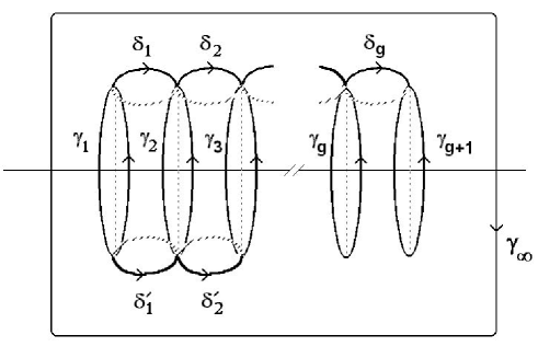
Figure 1: Projection of the cycles $\delta_{i}$ and $\gamma_{j}$ on the $x$-plane

Proposition 4.2

Assume that $f(x)$ is a real polynomial with simple roots.

1. $T_{\underline{h}}^{\mathbb{R}}$ is not empty if and only if $\underline{h}\in\mathcal{C}$.

2. The real structure $J_{2}$ acts on $J(C,\infty^{\pm})$ as $z\in\mathbb{C}^{g+1}/\Lambda_{2g+1}\longmapsto-\overline{z}\in\mathbb{C}^{g+1}/\Lambda_{2g+1}$, where $\overline{z}$ is the complex conjugation on $\mathbb{C}^{g+1}$.

Proof The definition of $J_{2}$ gives that if $(U,V,W)\in T_{C}$ and $J_{2}(U,V,W)=(U,V,W)$ then

$$V^{2}(x)+U(x)W(x)=|V(x)|^{2}+|U(x)|^{2}=f(x)\geq 0,\quad\forall x\in\mathbb{R}.$$

In If $f(x)$ vanishes then this zero is in fact double, and this is impossible. This shows that $f(x)$ is strictly positive. Reciprocally, if $\underline{h}\in\mathcal{C}$ then $J_{2}(\sum_{i=1}^{g+1}W_{i})=\sum_{i=1}^{g+1}W_{i}$.

Now let us determine the action of $J_{2}$ on $S^{g+1}\breve{C}$. Let $P_{1}=(x_{1},y_{1}),P_{2}=(x_{2},y_{2}),...,P_{g+1}=(x_{g+1},y_{g+1})$ be generic points on $\breve{C}$. Let us consider the curve $X=\{(x,y)\in\mathbb{C}^{2}:\quad y=V(x)\}$ where $V(x)$ is the Lagrange polynomial of degree $g$ such that $X$ contains $P_{1},P_{2},...,P_{g+1}$. The intersection points between $\breve{C}$ and $X$ are the points $P_{1},P_{2},...,P_{g+1},Q_{1},...,Q_{g+1}$. The points $Q_{i}=(x^{i},y^{i})$ are determined simply by $y^{i}=V(x^{i})$ where $x^{i}$ are roots of polynomial $V^{2}(x)-f(x)$ (which is the resultant of $y-V(x)$ and $y^{2}-f(x)$ with respect to $y$). We have

$((y-V(x))|_{C})=D_{1}+D_{2}-(g+1)(\infty^{+}+\infty^{-})$ where $\displaystyle D_{1}=\sum_{i=1}^{g+1}P_{i}$ and $\displaystyle D_{2}=\sum_{i=1}^{g+1}Q_{i}$,

$(y)=D_{0}+D^{\prime}_{0}-(g+1)(\infty^{+}+\infty^{-})$ where $\displaystyle D_{0}=\sum_{i=1}^{g+1}W_{i}$ and $\displaystyle D^{\prime}_{0}=\sum_{i=1}^{g+1}W_{g+1+i}$.

We get $((y-V(x))/y|_{C})=D_{1}+D_{2}-D_{0}-D^{\prime}_{0}$ and $(y-V(x))/y(\infty^{\pm})=1$ then $\displaystyle D_{1}-D_{0}\stackrel{{\scriptstyle\mathfrak{m}}}{{\bf{\sim}}}D^{\prime}_{0}-D_{2}$. Choose $D_{0}=\sum_{i=1}^{g+1}W_{i}$ as the base point of the Abel-Jacobi map $\mathcal{A}$.

Recall that if $S$ is real structure on $C$, then $S$ induces a transformation on the sheaves ${\mathcal{O}}_{C}$, $\Omega^{1}$, $\mathbb{Z}$.

$$\begin{array}[]{crcl}S^{*}:&\Gamma(U,{\mathcal{O}}_{C})&\longrightarrow&\Gamma(S(U),{\mathcal{O}}_{C})\\ &f&\longmapsto&\overline{foS}\\ \end{array}$$

We also denote by $S^{*}$ the transformation induced on $\Omega^{1}$. We shall say that $\alpha\in H^{0}(C,\Omega^{1})$ is $S$-real provided that $S^{*}\alpha=\alpha$. Moreover $S$ induces an involution on $C_{1}(C,\mathbb{Z})$ (the group of topological 1-cycles). If $\alpha\in H^{0}(C,\Omega^{1})$ and $c\in C_{1}(C,\mathbb{Z})$ then $\displaystyle\int_{c}S^{*}\alpha=\overline{\int_{S(c)}\alpha}$. If $\alpha$ is $S$-real, we get $\displaystyle\int_{c}\alpha=\overline{\int_{S(c)}\alpha}$. We shall say $c\in H_{1}(C,\mathbb{Z})$ is $S$-real ($S$-imaginary) if $S(c)=c$ ($S(c)=-c$ ).

The differential one-forms $x^{i}dx/y$ on $C$ are real (for the usual real structure), and if we denote $\omega=\left(dx/y,xdx/y,...,x^{g}dx/y\right)$ then

$$\int_{D_{0}}^{J_{2}(D_{1})}\omega=\overline{\int_{D^{\prime}_{0}}^{D_{2}}\omega}=-\overline{\int_{D_{2}}^{D^{\prime}_{0}}\omega}=-\overline{\int_{D_{0}}^{D_{1}}\omega}.$$

Therefore the involution $J_{2}$ acts on $J(C,\infty^{\pm})$ as $z\longmapsto J_{2}(z)=-\overline{z}$, $z\in\mathbb{C}^{g+1}/\Lambda_{2g+1}$, where $\displaystyle z=\int_{D_{0}}^{D_{1}}\omega$ and $\displaystyle J_{2}(z)=\int_{D_{0}}^{J_{2}(D_{1})}\omega$.

Theorem 4.1

$T_{\underline{h}}^{\mathbb{R}}\subset\mathbb{C}^{g+1}/\Lambda_{2g+1}$ is topologically a $(g+1)$-torus and its periods are generated by $e_{i},\quad i\in\{1,2,...,g+1\}$.

Proof The fact that $T_{\underline{h}}^{\mathbb{R}}$ is compact and connected is proved by Previato [27]. Consider the image of $T_{\underline{h}}^{\mathbb{R}}$ in $J(C,\infty^{\pm})$ under the Abel-Jacobi map. As $\omega$ is real and $\gamma_{i}$ are imaginary cycles, then $e_{i}\in\mathbb{C}^{g+1}$ are purely imaginary vectors. We shall determine the action of $J_{2}$ on $H_{1}(\breve{C}_{h},\mathbb{Z})$ and hence on the period lattice $\Lambda_{2g+1}$. Let us choose a base of $H_{1}(\breve{C}_{h},\mathbb{Z})$ as on figure 1.

Under the standard anti-holomorphic involution $\delta_{j}$ is sent to $\delta^{\prime}_{j}$ which is homologous to $\displaystyle\delta_{j}-\gamma_{\infty}-\sum_{i=1,\\ i\neq j,\\ i\neq j+1}^{g+1}\gamma_{i}$. As $\displaystyle\gamma_{\infty}\equiv-\sum_{i=1}^{g+1}\gamma_{i}$ then $\delta_{j}^{\prime}\equiv\delta_{j}+\gamma_{j}+\gamma_{j+1}$. Thus

$\overline{f_{j}}=f_{j}+e_{j}+e_{j+1}$ and $J_{2}(f_{j})=-\overline{f_{j}}=-f_{j}-e_{j}-e_{j+1}$.

Denote by $z\in\mathbb{C}^{g+1}$, $\Re(z)\in\mathbb{R}^{g+1}$ the real part of $z$.

Complete further $\{e_{1},...,e_{g+1},f_{1},...,f_{g}\}$ to a basis of $\mathbb{C}^{g+1}$ by $\{e_{1},...,e_{g+1},f_{1},...,f_{g},f_{g+1}\}$ under the condition that
$\{\Re{(f_{1})},...,\Re{(f_{g+1})},f_{g+1}\}$ is a basis of $\mathbb{R}^{g+1}$. The fixed points of $J_{2}$ in $\mathbb{C}^{g+1}$ are given by

$$J_{2}z=z,\mbox{ where }J_{2}=\left(\begin{array}[]{cc}Id_{g+1}&-A\\ 0&-Id_{g+1}\\ \end{array}\right)\mbox{ and }A=\left(\begin{array}[]{cccccc}1&0&0&\ldots&0&0\\ 1&1&0&\ldots&0&0\\ 0&1&1&\ldots&0&0\\ \vdots&&1&\ldots&0&0\\ &&&&1&0\\ 0&\ldots&&&1&0\\ \end{array}\right).$$

If $z\in\mathbb{C}^{g+1}/{\mathbb{Z}\{e_{1},...,e_{g+1},f_{1},...,f_{g+1}\}}$ the only possible solutions are

$\forall(q_{1},...,q_{g+1})\in S^{g+1},\quad\forall j\in\{1,2,...,g\}\quad p_{j}\equiv 0\mbox{ mod }f_{j}\mbox{ and }\quad 2p_{g+1}\equiv 0\mbox{ mod }f_{g+1}$.

Assume that the vector $f_{g+1}$ tends to infinity, and get

$\forall(q_{1},...,q_{g+1})\in S^{g+1},\quad\forall j\in\{1,2,...,g\},\quad p_{j}\equiv 0\mbox{ mod }f_{j}$.

Finally $T_{\underline{h}}^{\mathbb{R}}$ is generated by $e_{i}$ for $i\in\{1,2,...,g+1\}$.

5 The Monodromy

5.1 The case $g=0$

The system (1) is

$$\frac{d}{dt}\Gamma_{0}=\left[\Gamma_{0},\Omega\right]$$

or equivalently

$$\left\{\begin{array}[]{ccc}\dot{\omega_{1}}&=&-m\omega_{2}\omega_{3}\\ \dot{\omega_{2}}&=&m\omega_{1}\omega_{3}\\ \dot{\omega_{3}}&=&0\\ \end{array}\right.$$

It is a Hamiltonian system with one degree of freedom with Poisson structure

$$\begin{array}[]{c||ccc}\{.,.\}&\omega_{1}&\omega_{2}&\omega_{3}\\ \hline\cr\hline\cr\omega_{1}&0&-(1+m)\omega_{3}&\omega_{2}/(1+m)\\ \omega_{2}&(1+m)\omega_{3}&0&-\omega_{1}/(1+m)\\ \omega_{3}&-\omega_{2}/(1+m)&\omega_{1}/(1+m)&0\\ \end{array}$$

and Hamiltonian

$$H=H_{0}-\frac{m}{2(1+m)}H_{-1}^{2}=\frac{1}{2}\left(\omega_{1}^{2}+\omega_{2}^{2}+(1+m)\omega_{3}^{2}\right),$$

where

$$H_{-1}=(1+m)\omega_{3}$$

is a first integral and

$$H_{0}=\frac{1}{2}\left(\omega_{1}^{2}+\omega_{2}^{2}+(1+m)^{2}\omega_{3}^{2}\right)$$

is a Casimir function. The spectral curve associated to the Lax pair (4) is given by the polynomial

$$y^{2}-f(x)=y^{2}-U(x)W(x)-V^{2}(x)=y^{2}-x^{2}-2h_{-1}x-\left(2h+\frac{m}{1+m}h_{-1}^{2}\right)=0.$$

It is a genus zero curve and its generalized Jacobian is $\mathbb{C}^{*}$. It is identified to the invariant manifold of the system. The spectral curve as well the corresponding Lagrangian fibration have no monodromy.

5.2 The case $g=1$ (the Lagrange top)

The system (1) is

$$\frac{d}{dt}\left(\chi\lambda+\Gamma_{0}-\Gamma_{1}\lambda^{-1}\right)=\left[\chi\lambda+\Gamma_{0}-\Gamma_{1}\lambda^{-1},\chi\lambda+\Omega\right].$$ (5)

or equivalently

$$\frac{d}{dt}\Gamma_{0}=\left[\Gamma_{0},\Omega\right]-\left[\Gamma_{1},\chi\right],$$

$$\frac{d}{dt}\Gamma_{1}=\left[\Gamma_{1},\Omega\right].$$

If we denote

$$\Gamma_{1}=\left(\begin{array}[]{ccc}0&-\gamma_{3}&\gamma_{2}\\ \gamma_{3}&0&-\gamma_{1}\\ -\gamma_{2}&\gamma_{1}&0\\ \end{array}\right)$$

then the system takes the form

$$\left\{\begin{array}[]{ccllccl}\dot{\omega_{1}}&=&-m\omega_{2}\omega_{3}-\gamma_{2},&&\dot{\gamma_{1}}&=&\gamma_{2}\omega_{3}-\gamma_{3}\omega_{2},\\ \dot{\omega_{2}}&=&m\omega_{1}\omega_{3}+\gamma_{1},&&\dot{\gamma_{2}}&=&\gamma_{3}\omega_{1}-\gamma_{1}\omega_{3},\\ \dot{\omega_{3}}&=&0,&&\dot{\gamma_{3}}&=&\gamma_{1}\omega_{2}-\gamma_{2}\omega_{1}.\\ \end{array}\right.$$

It is a two degrees of freedom integrable Hamiltonian system with Poisson structure

$$\begin{array}[]{c||cccccc}\{.,.\}&\omega_{1}&\omega_{2}&\omega_{3}&\gamma_{1}&\gamma_{2}&\gamma_{3}\\ \hline\cr\hline\cr\omega_{1}&0&-(1+m)\omega_{3}&\omega_{2}/(1+m)&0&-\gamma_{3}&\gamma_{2}\\ \omega_{2}&(1+m)\omega_{3}&0&-\omega_{1}/(1+m)&\gamma_{3}&0&-\gamma_{1}\\ \omega_{3}&-\omega_{2}/(1+m)&\omega_{1}/(1+m)&0&-\gamma_{2}/(1+m)&\gamma_{1}/(1+m)&0\\ \gamma_{1}&0&-\gamma_{3}&\gamma_{2}/(1+m)&0&0&0\\ \gamma_{2}&\gamma_{3}&0&-\gamma_{1}/(1+m)&0&0&0\\ \gamma_{3}&-\gamma_{2}&\gamma_{1}/(1+m)&0&0&0&0\\ \end{array}$$ (6)

and Hamiltonian

$$H=\frac{1}{2}\left(\omega_{1}^{2}+\omega_{2}^{2}+(1+m)\omega_{3}^{2}\right)-\gamma_{3}.$$

The second first integral is

$$H_{-1}=(1+m)\omega_{3}.$$

and the Casimir functions are

$$H_{1}=-\omega_{1}\gamma_{1}-\omega_{2}\gamma_{2}-(1+m)\omega_{3}\gamma_{3},$$

$$H_{2}=\frac{1}{2}\left(\gamma_{1}^{2}+\gamma_{2}^{2}+\gamma_{3}^{2}\right).$$

The spectral curve $\widetilde{C}$ is given by

$$y^{2}-f(x)=y^{2}-x^{4}-2h_{-1}x^{3}-\left(2h+\frac{m}{1+m}h_{-1}^{2}\right)x^{2}-2h_{1}x-2h_{2}=0.$$ (7)

The system (6) describes the motion of a symmetric rigid body spinning about its axis whose base point is fixed ((fig. 2). A constant vertical gravitational force acts on the center of mass of the top, which lies on its axis. The vector $\gamma$ is the unit vector $e_{z}$ expressed in body coordinates, while the vector $\omega$ is the angular velocity of the body. For more details we refer the reader to [3, 7]. For completeness we give below the Lagrangean function in Euler coordinates $\phi,\psi,\theta$ (shown of fig. 2), which are local coordinates on an open subset of the configuration space $SO(3)$. This problem will have three degrees of freedom. It has three first integrals : the total energy $E$, the projection $M_{z}$ of the angular momentum on the vertical, the projection $M_{3}$ of the angular momentum vector on the $e_{3}$ axis (figure 2).

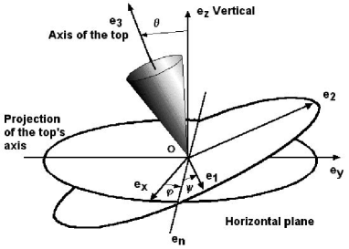
Figure 2: the Lagrange top

Let $A=B\neq C$ be the moments of inertia of the body at $0$, and let $e_{1},e_{2}$ and $e_{3}$ the unit vectors of a right moving co-ordinate system connected to the body, directed along the principal axes at fixed point $0$. We note by $\omega$ the angular velocity of the top which is expressed in terms of the derivates of the Euler angles by the formula (cf [3])

$$\omega=\omega_{1}e_{1}+\omega_{2}e_{2}+\omega_{3}e_{3}=\dot{\theta}e_{1}+(\dot{\phi}\sin\theta)e_{2}+(\dot{\psi}+\dot{\phi}\cos\theta)e_{3}$$

where $0<\phi<2\pi,0<\psi<2\pi$ and $0<\theta<\pi$. Since $T=\frac{1}{2}(A\omega_{1}^{2}+B\omega_{2}^{2}+C\omega_{3}^{2})$, the kinetic energy is given

$$T=\frac{A}{2}(\dot{\theta}^{2}+\dot{\phi}^{2}\sin^{2}\theta)+\frac{C}{2}(\dot{\psi}+\dot{\phi}\cos\theta)^{2}$$

and the potential energy is equal to

$$U={\bf m}gl\cos\theta$$

where $l$ is the distance between the fixed point and the center of mass of the top. The Lagrangian function reads

$$L=T-U=\frac{A}{2}(\dot{\theta}^{2}+\dot{\phi}^{2}\sin^{2}\theta)+\frac{C}{2}(\dot{\psi}+\dot{\phi}\cos\theta)^{2}-{\bf m}gl\cos\theta.$$

Let $p_{\phi},p_{\psi}$ and $p_{\theta}$ be the conjugate moments. To the cyclic co-ordinates $\phi$ and $\psi$ correspond the first integrals

$$p_{\phi}=\frac{\partial L}{\partial\dot{\phi}}=M_{z}=\dot{\phi}(A\sin^{2}\theta+C\cos^{2}\theta)+\dot{\psi}C\cos\theta,$$

$$p_{\psi}=\frac{\partial L}{\partial\dot{\psi}}=M_{3}=\left(\dot{\phi}\cos\theta+\dot{\psi}\right)C.$$

The last conjugate moment $p_{\theta}$ is equal to $p_{\theta}=A\dot{\theta}.$ The momentum mapping of the Lagrange top is

$$F:T^{*}V\longrightarrow\mathbb{R}^{3}$$

$$(\phi,\psi,\theta,p_{\phi},p_{\psi},p_{\theta})\longmapsto(E,M_{3},M_{z})$$

Eliminating $\dot{\phi}$ and $\dot{\psi}$, we get the total energy $E$ of the system as

$$E=\frac{1}{2A}{p_{\theta}}^{2}+\frac{M_{3}^{2}}{2C}+\frac{(M_{z}-M_{3}\cos\theta)^{2}}{2A\sin^{2}\theta}+{\bf m}gl\cos\theta.$$

Let

$$a_{1}=\frac{2M_{3}}{A},a_{2}=\frac{2E}{A}+\frac{M_{3}^{2}}{A}\left(\frac{1}{A}-\frac{1}{C}\right),a_{3}=\frac{2M_{z}}{A}.$$

and obviously $(E,M_{3},M_{z})\longrightarrow(a_{1},a_{2},a_{3})$ is a bi-polynomial map. Moreover we shall assume that

$$A={{\bf m}gl}.$$

Then action variables are obviously given by [2] :

$$I_{1}=\frac{A}{2\pi}\oint_{\gamma}\frac{\sqrt{g(u)}}{1-u^{2}}du,I_{2}=M_{3},I_{3}=M_{z}$$

where

$$g(u)=2u^{3}-a_{2}u^{2}+(a_{1}a_{3}/2-2)u+a_{2}-(a_{1}^{2}+a_{3}^{2})/4$$

and the cycle $\gamma$ is defined on figure 3.b. It is well known [36] that for a real motion of Lagrange top, the polynomial $g(u)$ has exactly two real roots $u_{1}$ and $u_{2}$ on the interval $-1\leq u\leq 1$ and one for $u>1$ (figure 3.a).

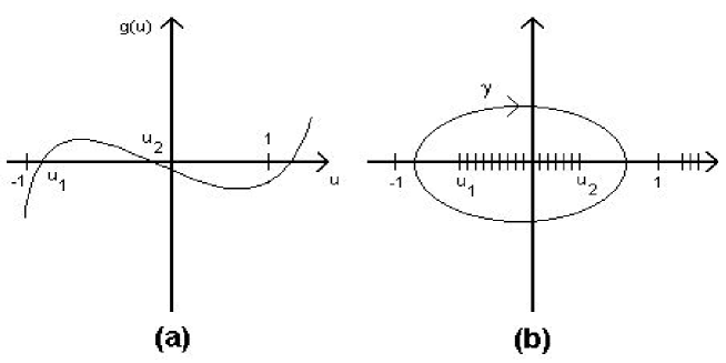
Figure 3: (a) graph of the function $g(u)$ and (b) projection of the cycle $\gamma$ on the $u$-plane

The linear change of variables

$$u=-2\xi+\frac{a_{2}}{6},v=-2\sqrt{-1}\eta.$$

transforms the curve $\Gamma$ (*) to the curve

$$\Gamma^{\prime}=\{\eta^{2}=4\xi^{3}-i\xi-j\}$$

where

$$i=1-\frac{a_{1}a_{3}}{4}+\frac{a_{2}^{2}}{12},j=\frac{a_{2}}{6}+\frac{a_{1}a_{2}a_{3}}{48}-\frac{a_{1}^{2}}{16}-\frac{a_{2}^{3}}{216}-\frac{a_{3}^{2}}{16}.$$

Subsequently we shall consider two elliptic curves $\Gamma^{\prime}$ and

$$C=\{(x,y)\in\mathbb{C}^{2}:\quad y^{2}=x^{4}+a_{1}x^{3}+a_{2}x^{2}+a_{3}x+1\}.$$

Remark 1

$C$ is nothing but the curve $\tilde{C}$ (7), where

$$A=1,\quad E=H,\quad M_{3}=H_{-1},\quad M_{z}=H_{2},\quad m=C-1.$$

The curves $C$ and $\Gamma$ are isomorphic, more precisely $\Gamma^{\prime}$ as the Jacobian $J(C)$ of $C$ [37]. The birational mapping identifying $C$ and $\Gamma^{\prime}$ is given by

$$(x,y)\longmapsto\left(\xi=\frac{A_{1}}{x-r_{0}}+\frac{A_{2}}{2},\eta=\frac{yA_{1}}{(x-r_{0})^{2}}\right)$$

where $r_{0}$ is a root of $f(x)$ such that its real part is positive and $A_{1}=r_{0}^{3}+\frac{3}{4}a_{1}r_{0}^{2}+\frac{1}{2}a_{2}r_{0}+\frac{1}{4}a_{3},A_{2}=r_{0}^{2}+\frac{1}{2}a_{1}r_{0}+\frac{1}{6}a_{2}$. The map (**) sends the root $r_{0}$ to $\infty$ and then translates the barycenter of the three remaining roots into the origin [5]. Using (**) it is easy to check

$$\frac{d\xi}{\eta}=-\frac{dx}{y}.$$

Now we are going to study the discriminant locus $\Delta\subset\mathbb{R}^{3}$ of the polynomial $f(x)=x^{4}+a_{1}x^{3}+a_{2}x^{2}+a_{3}x+1$. We denote $\Delta_{c}=\Delta\cap\{a_{3}$=c$\}\subset\mathbb{R}^{2}$ in the $(a_{1},a_{2})$-plane. Let us consider the following cases :

• If $f(x)$ has a real double root $u$ then

  $$f(x)=(x-u)^{2}(x^{2}+\alpha x+\beta),\alpha\in\mathbb{R},\beta,u\in\mathbb{R}\backslash\{0\}.$$

  Hence

  $$\left\{\begin{array}[]{c}a_{1}=(c+{2}/{u})/u^{2}-2u\\ a_{2}={-3}/{u^{2}}-{2c}/{u}+u^{2}\end{array}\right.$$

  $\Delta_{c}$ is parameterized by $u\in\mathbb{R}\backslash\{0\}$.

• If $f(x)$ has a real triple root $u$ then

  $$f(x)=(x-u)^{3}(x-\alpha),\alpha,u\in\mathbb{R}\backslash\{0\}.$$

  • If $c=\pm 4$ then $u=\mp 1$ is a real quadruple root. It is the point $(a_{1},a_{2})=(\pm 4,6)$.

  • If $|c|>4$ then there are two possibilities for $u$, moreover $u$ has the sign of $-c$.

  • If $|c|<4$ then $f$ can not have a real triple root.

• If $f(x)$ has two double roots then

  $$f(x)=(x^{2}+\alpha x+\beta)^{2},\alpha\in\mathbb{R},\beta\in\mathbb{R}\backslash\{0\}.$$

  • If $(\alpha,\beta)=(-c/2,-1)$ then $f$ have two real distinct double roots of opposite sign. Therefore the two branchs of $\Delta_{c}$ have an intersection point at $(a_{1},a_{2})=(-c,-2+c^{2}/4)$.

  • If $(\alpha,\beta)=(c/2,1)$ then

    • If $|c|>4$ then we have two different real double roots of the same sign as $-c$. They represent a normal crossing of $\Delta_{c}$ with coordinates $(a_{1},a_{2})=(c,2+c^{2}/4).$

    • If $|c|<4$ then we have a pair of complex conjugate double roots. They represent an isolated point of the real discriminant locus with coordinates $(a_{1},a_{2})=(c,2+c^{2}/4)$.

The sections $\Delta_{c}$ of the dicriminant locus $\Delta$ are shown on figure 4. Let $\mathcal{C}_{c}$ be the connected component of the complement to $\Delta_{c}$ in $\mathbb{R}^{2}$, in which $f(x)$ has no real root.

$$\mathcal{C}=\left\{(a_{1},a_{2},a_{3})\in\mathbb{R}^{3}:\quad(a_{1},a_{2})\in\mathcal{C}_{a_{3}}\mbox{ and }|a_{3}|<4\right\}$$

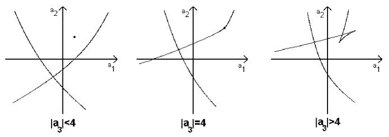
Figure 4: the discriminant locus of $f(x)$

Lemma 5.1

We have

$$I_{1}=\frac{A\sqrt{-1}}{2\pi}\oint_{\gamma_{1}}\frac{y}{x^{2}}dx$$

where $y^{2}=x^{4}+a_{1}x^{3}+a_{2}x^{2}+a_{3}x+1$ and the cycle $\gamma_{1}$ is defined on figure 5.

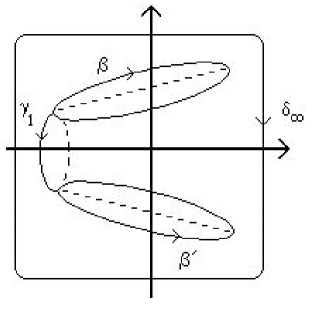
Figure 5: projection of the cycles $\gamma_{1},\delta_{1},\delta_{1}^{\prime}$ and $\gamma_{\infty}$ on the $x$-plane

Proof We have

$$\frac{\partial I_{1}}{\partial a_{2}}=\frac{A}{4\pi}\oint_{\gamma}\frac{du}{v}=-\frac{A\sqrt{-1}}{4\pi}\oint_{\gamma}\frac{d\xi}{\eta}\stackrel{{\scriptstyle(***)}}{{=}}\frac{A\sqrt{-1}}{4\pi}\oint_{\gamma_{1}}\frac{dx}{y}=\frac{A\sqrt{-1}}{2\pi}\frac{\partial}{\partial a_{2}}\left(\oint_{\gamma_{1}}\frac{y}{x^{2}}dx\right).$$

Then

$$I_{1}=\frac{A\sqrt{-1}}{2\pi}\oint_{\gamma_{1}}\frac{y}{x^{2}}dx+g(a_{1},a_{3})$$

where $g(a_{1},a_{3})$ is a function. To compute $g(a_{1},a_{3})$, we note that for any fixed $(a_{1},a_{3})$ such that the polynomial $f(x)$ has no real root, we may continuously deform $a_{2}$ in such a way, that $(a_{1},a_{2},a_{3})$ lies on $\Delta$. But under such a deformation the cycle $\gamma_{1}(a_{1},a_{2},a_{3})$ vanishes. And hence $I_{1}(a_{1},a_{2},a_{3})=0$ and $\oint_{\gamma_{1}}{y}dx/{x^{2}}=0$ which implies $g(a_{1},a_{3})=0$.

5.2.1 The monodromy of Lagrange top

Let $F:T^{*}V\longrightarrow\mathbb{R}^{3}$ be the moment map of the Lagrange top, where $V=SO(3)$. We consider the fibration

$$\widetilde{F}:T^{*}V\backslash F^{-1}(\Delta)\longrightarrow\mathbb{R}^{3}\backslash\Delta.$$

This is a proper topological fibration, the fibers of which are diffeomorphic to three-tori ${{\bf T}}^{3}$. We consider the real monodromy of $\widetilde{F}$ defined as the action of $\pi_{1}(\mathbb{R}^{3}\backslash\Delta,c)$ on $H_{1}(\widetilde{F}^{-1}(c),\mathbb{Z})$, $c=(c_{1},c_{2},c_{3})\in\mathbb{R}^{3}\backslash\Delta$. We choose now a basis $\alpha_{1},\alpha_{2}$ and $\alpha_{3}$ of $H_{1}(\widetilde{F}^{-1}(c),\mathbb{Z})$ in the following way :

• For $\alpha_{1}$ we take the path on $\widetilde{F}^{-1}(c)$ defined by fixing $\phi,\psi$. $\theta,p_{\theta}$ make one circle on the curve defined by the equation

  $$c_{1}=\frac{1}{2A}{p_{\theta}}^{2}+\frac{c_{2}^{2}}{2C}+\frac{(c_{3}-c_{2}\cos\theta)^{2}}{2A\sin^{2}\theta}+{\bf m}gl\cos\theta$$

• For $\alpha_{2}$ we fix $\theta,p_{\theta}$ and $\phi$ and $\psi$ run through the interval $[0,2\pi]$.

• For $\alpha_{3}$ we fix $\theta,p_{\theta}$ and $\psi$ and $\phi$ run through the interval $[0,2\pi]$.

With such a choice of basis of $H_{1}(\widetilde{F}^{-1}(c),\mathbb{Z})$, the action variables are given by

$$I_{i}=\frac{1}{2\pi}\oint_{\alpha_{i}}\sigma,i=1,2,3.$$

where $\sigma=p_{\theta}d\theta+p_{\phi}d\phi+p_{\psi}d\psi$ is the fundamental one-form on $T^{*}V$.

Theorem (R. Cushman) [12, 7] If $z_{0}\in\mathcal{C}$ then $\pi_{1}(\mathbb{R}^{3}\backslash D,z_{0})=\mathbb{Z}$ and the real monodromy of $F$ can be represented, on the basis $\alpha_{i}$ (defined above) for $H_{1}(F^{-1}(c),\mathbb{Z})$, by the matrix

$$\left(\begin{array}[]{ccc}1&0&0\\ 1&1&0\\ 0&0&1\\ \end{array}\right).$$

Proof The proof of this theorem will follow from the following elementary

Lemma 5.2

The real discriminant locus of the real polynomial $f(x)=(x^{2}+1)^{2}+(a_{1}x+a_{2})x^{2}$ in a small neighborhood of the origin in $\mathbb{R}^{2}\{a_{1},a_{2}\}$ consists of the point $(0,0)$. When $(a_{1},a_{2})$ makes one turn around $(0,0)$ in a negative direction then the roots of $f(x)$ exchange their places as it is shown on figure 6.

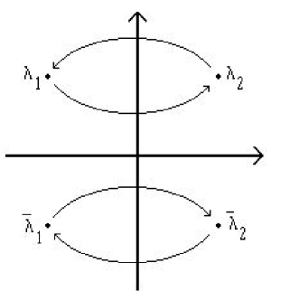
Figure 6: the $x$-plane

Proof

The proof is straightforward.

Remark 2

For $(a_{1},a_{2})\in\mathbb{R}^{2}$ sufficiently small, the real polynomial $f(x)$ has either two double roots or it has no double root at all. Hence the real discriminant locus of $f(x)$ is of codimension two and hence it is the point $(0,0)$. This phenomenon has a more general nature, see Looijenga [22].

To compute the monodromy of the action variables (equivalently, the monodromy of the homology bundle of the Lagragian fibration $\tilde{F}$), we shall consider the monodromy of the homology bundle of the Milnor fibration $\mathcal{B}$ of the polynomial $y^{2}-x^{4}-a_{1}x^{3}-a_{2}x^{2}-a_{3}x-1$. This is a fibration with fiber $\widetilde{C}$ over $\mathbb{R}^{3}\backslash\Delta$, defined by

$$\mathcal{B}\longrightarrow\mathbb{R}^{3}\backslash\Delta$$

$$\{y^{2}=x^{4}+a_{1}x^{3}+a_{2}x^{2}+a_{3}x+1\}\longmapsto(a_{1},a_{2},a_{3}).$$

$\pi_{1}(\mathbb{R}^{3}\backslash\Delta,z_{0})$ is not trivial if and only if $z_{0}\in\mathcal{C}$.

Denote $P_{0}=(c,2+c^{2}/4)$ on the $(a_{1},a_{2})$-plane, and consider a simple negatively oriented (because the map $(E,M_{3},M_{z})\longrightarrow(a_{1}(E,M_{3},M_{z}),a_{2}(E,M_{3},M_{z}),a_{3}(E,M_{3},M_{z}))$ reverse the orientation) loop $\kappa$ around $P_{0}$, figure 7.

Figure 7: the loop $\kappa\in\pi_{1}(\mathcal{C}_{c},z_{0})$

This defines $\kappa$ as a loop in $\mathbb{R}^{3}\backslash\Delta$ with $z_{0}\in\mathcal{C}$ as base point. It is possible to deform continuously $\kappa$ to a loop (with the same orientation) contained in $\mathcal{C}\cap\{a_{3}=0\}$. The monodromy of roots of $f(x)$ induces the monodromy of cycles in $H_{1}(\widetilde{C},\mathbb{Z})$. This situation is described in figures 8.a and 8.b.

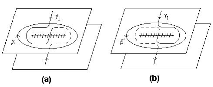
Figure 8: the cycle $\gamma_{1}$ (a) and (b)

Let $\gamma_{1}^{\prime}$ be the image of $\gamma_{1}$ after making one turn along $\kappa$ in negative direction. Then the classical Picard-Lefschetz formula [4] implies $\gamma_{1}^{\prime}\equiv\gamma_{1}+\delta_{1}-\delta_{1}^{\prime}$ and moreover we have $\gamma_{\infty}\equiv\delta_{1}-\delta_{1}^{\prime}$ where the projections of $\delta_{1},\delta_{1}^{\prime}$ and $\gamma_{\infty}$ on the $x$-plane are shown on figure 5. That is to say

$$I_{1}^{\prime}=\frac{A\sqrt{-1}}{2\pi}\oint_{\gamma_{1}^{\prime}}\frac{\sqrt{f(x)}}{x^{2}}dx=\frac{A\sqrt{-1}}{2\pi}\oint_{\gamma_{1}}\frac{\sqrt{f(x)}}{x^{2}}dx+\frac{A\sqrt{-1}}{2\pi}\oint_{\gamma_{\infty}}\frac{\sqrt{f(x)}}{x^{2}}dx$$

and

$$\oint_{\gamma_{\infty}}\frac{\sqrt{f(x)}}{x^{2}}dx=2\sqrt{-1}\pi\mbox{ residue}_{x=\infty}\left(\frac{\sqrt{f(x)}}{x^{2}}dx\right)=-\sqrt{-1}\pi a_{1}.$$

We see that $I_{1}$ is transformed to $I_{1}+I_{2}$.

5.3 The case $g=2$

For this case the system (1) is

$$\frac{d}{dt}\left(\chi\lambda+\Gamma_{0}-\Gamma_{1}\lambda^{-1}-\Gamma_{2}\lambda^{-2}\right)=\left[\chi\lambda+\Gamma_{0}-\Gamma_{1}\lambda^{-1}-\Gamma_{2}\lambda^{-2},\chi\lambda+\Omega\right].$$ (8)

As above we put

$$\Gamma_{1}=\left(\begin{array}[]{ccc}0&-\gamma_{3}&\gamma_{2}\\ \gamma_{3}&0&-\gamma_{1}\\ -\gamma_{2}&\gamma_{1}&0\\ \end{array}\right),\quad\Gamma_{2}=\left(\begin{array}[]{ccc}0&-\theta_{3}&\theta_{2}\\ \theta_{3}&0&-\theta_{1}\\ -\theta_{2}&\theta_{1}&0\\ \end{array}\right).$$

In these notations

$$\frac{d}{dt}\Gamma_{0}=\left[\Gamma_{0},\Omega\right]-\left[\Gamma_{1},\chi\right],$$

$$\frac{d}{dt}\Gamma_{1}=\left[\Gamma_{1},\Omega\right]+\left[\Gamma_{2},\chi\right],$$

$$\frac{d}{dt}\Gamma_{2}=\left[\Gamma_{2},\Omega\right].$$

or also

$$\left\{\begin{array}[]{ccllccllccl}\dot{\omega_{1}}&=&-m\omega_{2}\omega_{3}-\gamma_{2},&&\dot{\gamma_{1}}&=&\gamma_{2}\omega_{3}-\gamma_{3}\omega_{2}+\theta_{2},&&\dot{\theta_{1}}&=&\omega_{3}\theta_{2}-\omega_{2}\theta_{3},\\ \dot{\omega_{2}}&=&m\omega_{1}\omega_{3}+\gamma_{1},&&\dot{\gamma_{2}}&=&\gamma_{3}\omega_{1}-\gamma_{1}\omega_{3}-\theta_{1},&&\dot{\theta_{2}}&=&\omega_{1}\theta_{3}-\omega_{3}\theta_{1},\\ \dot{\omega_{3}}&=&0,&&\dot{\gamma_{3}}&=&\gamma_{1}\omega_{2}-\gamma_{2}\omega_{1},&&\dot{\theta_{3}}&=&\omega_{2}\theta_{1}-\omega_{1}\theta_{2}.\\ \end{array}\right.$$

Let us consider this Poisson structure

$$\begin{array}[]{c||ccccccccc}\{.,.\}&\omega_{1}&\omega_{2}&\omega_{3}&\gamma_{1}&\gamma_{2}&\gamma_{3}&\theta_{1}&\theta_{2}&\theta_{3}\\ \hline\cr\hline\cr\omega_{1}&0&-(1+m)\omega_{3}&\frac{\omega_{2}}{1+m}&0&-\gamma_{3}&\gamma_{2}&0&-\theta_{3}&\theta_{2}\\ \omega_{2}&(1+m)\omega_{3}&0&-\frac{\omega_{1}}{1+m}&\gamma_{3}&0&-\gamma_{1}&\theta_{3}&0&-\theta_{1}\\ \omega_{3}&-\frac{\omega_{2}}{1+m}&\frac{\omega_{1}}{1+m}&0&-\frac{\gamma_{2}}{1+m}&\frac{\gamma_{1}}{1+m}&0&-\frac{\theta_{2}}{1+m}&\frac{\theta_{1}}{1+m}&0\\ \gamma_{1}&0&-\gamma_{3}&\frac{\gamma_{2}}{1+m}&0&\theta_{3}&-\theta_{2}&0&0&0\\ \gamma_{2}&\gamma_{3}&0&-\frac{\gamma_{1}}{1+m}&-\theta_{3}&0&\theta_{1}&0&0&0\\ \gamma_{3}&-\gamma_{2}&\frac{\gamma_{1}}{1+m}&0&\theta_{2}&-\theta_{1}&0&0&0&0\\ \theta_{1}&0&-\theta_{3}&\frac{\theta_{2}}{1+m}&0&0&0&0&0&0\\ \theta_{2}&\theta_{3}&0&-\frac{\theta_{1}}{1+m}&0&0&0&0&0&0\\ \theta_{3}&-\theta_{2}&\theta_{1}&0&0&0&0&0&0&0\\ \end{array}$$

The Hamiltonian function corresponding to (8) is

$$H=\frac{1}{2}\left(\omega_{1}^{2}+\omega_{2}^{2}+(1+m)\omega_{3}^{2}\right)-\gamma_{3}.$$

The Hamiltonian functions in involution with $H$ are

$$H_{-1}=(1+m)\omega_{3},$$

$$H_{1}=-\omega_{1}\gamma_{1}-\omega_{2}\gamma_{2}-(1+m)\omega_{3}\gamma_{3}-\theta_{3}.$$

The Casimir functions are

$$H_{2}=\frac{1}{2}\left(\gamma_{1}^{2}+\gamma_{2}^{2}+\gamma_{3}^{2}\right)-\omega_{1}\theta_{1}-\omega_{2}\theta_{2}-(1+m)\omega_{3}\theta_{3},$$

$$H_{3}=\gamma_{1}\theta_{1}+\gamma_{2}\theta_{2}+\gamma_{3}\theta_{3},$$

$$H_{4}=\frac{1}{2}\left(\theta_{1}^{2}+\theta_{2}^{2}+\theta_{3}^{2}\right).$$

The spectral curve $\widetilde{C}$ is given by

$$y^{2}=x^{6}+2h_{-1}x^{5}+\left(2h+\frac{m}{1+m}h_{-1}^{2}\right)x^{4}+2h_{1}x^{3}+2h_{2}x^{2}+2h_{3}x+2h_{4}.$$

The monodromy of cycles on spectral curve $\widetilde{C}$ generates the monodromy of momentum map associated to the system (8).

5.3.1 The discriminant of $(x^{2}+1)^{3}+x^{3}(ax^{2}+bx+c)$

Let us consider the real discriminant $\Delta(a,b,c)$ of the polynomial $P(x)=(x^{2}+1)^{3}+x^{3}(ax^{2}+bx+c)$ when $(a,b,c)$ is closed to $(0,0,0)$. Assume that

$$P(x)=\left({x}^{2}+{c_{1}}\,x+{c_{2}}\right)^{2}\left({x}^{2}+{d_{1}}\,x+{d_{2}}\right)$$

and hence

$$\left\{\displaystyle\begin{array}[]{ccl}a&=&2\alpha(c_{2}-1)(c_{2}^{3}-1)/c_{2}^{3}\\ b&=&(c_{2}-1)^{3}(c_{2}^{3}+3c_{2}^{2}+3c_{2}+5)/3c_{2}^{2}\\ c&=&2\alpha(c_{2}-1)(2c_{2}^{3}+3c_{2}-5)/3c_{2}^{2}\\ c_{1}&=&\alpha(c_{2}-1)\\ d_{1}&=&-2\alpha(c_{2}-1)/c_{2}^{3}\\ d_{2}&=&c_{2}^{-2}\\ \end{array}\right.$$

where $\alpha$ verifies $3\alpha^{2}=c_{2}(c_{2}+2)$ and $c_{2}\neq 0$. The discriminant of $\left({x}^{2}+{c_{1}}\,x+{c_{2}}\right)^{2}$ is

$$\Delta_{1}(c_{2})=c_{1}^{2}-4c_{2}=1/3\,{c_{2}}\,\left(-10+{{c_{2}}}^{3}-3\,{c_{2}}\right)$$

and the discriminant of $\left({x}^{2}+{d_{1}}\,x+{d_{2}}\right)$ is

$$\Delta_{2}(c_{2})=d_{1}^{2}-4d_{2}=-4/3\,{\frac{2\,{{c_{2}}}^{3}+3\,{c_{2}}-2}{{{c_{2}}}^{5}}}$$

It is easy to check that $\Delta_{1}(c_{2})$ and $\Delta_{2}(c_{2})$ are negative when $c_{2}$ is close to $1$.Therefore the discriminant $\Delta(a,b,c)$ is parameterized near $(0,0,0)$ by

$$\left\{\displaystyle\begin{array}[]{ccl}a&=&2\alpha(c_{2}-1)(c_{2}^{3}-1)/c_{2}^{3}\\ b&=&(c_{2}-1)^{3}(c_{2}^{3}+3c_{2}^{2}+3c_{2}+5)/3c_{2}^{2}\\ c&=&2\alpha(c_{2}-1)(2c_{2}^{3}+3c_{2}-5)/3c_{2}^{2},c_{2}\in(0,\infty)\\ \end{array}\right.$$

(see figure 9). Denote the set on figure 9 by $\tilde{\Delta}$. The above shows that the connected component of the complement to the discriminant locus, in which the polynomial $(x^{2}+1)^{3}+x^{3}(ax^{2}+bx+c)$ has no real roots is homeomorphic to $\mathbb{R}^{3}\backslash\tilde{\Delta}$. Moreover this implies that, more generally, the connected component $\mathcal{C}\subset\mathbb{R}^{6}$ of the complement to the discriminant locus in which the spectral polynomial

$$x^{6}+2h_{-1}x^{5}+\left(2h+\frac{m}{1+m}h_{-1}^{2}\right)x^{4}+2h_{1}x^{3}+2h_{2}x^{2}+2h_{3}x+2h_{4}$$

has no real roots, is homeomorphic to $(\mathbb{R}^{3}\backslash\tilde{\Delta})\times\mathbb{R}^{3}$. Therefore we have the following

Lemma 5.3

The fundamental group of $\mathcal{C}$ is a free group with three generators.

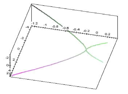
Figure 9: discriminant of $f(x)$

5.3.2 The monodromy of the generalized Lagrange top

The monodromy group of the top is a homomorphism from $\pi_{1}(\mathcal{C},p_{1})$ to $Aut(\mathbb{Z}^{3})$, where $\mathbb{Z}^{3}=H_{1}({{\bf T}}^{3},\mathbb{Z})$.

Consider the basis $\{\gamma_{1},\gamma_{3},\gamma_{\infty},\delta_{1},\delta_{2}\}$ of $H_{1}(\widetilde{C},\mathbb{Z})$ shown on (fig 5.3.2). The cycles generating the Liouville tori are the cycles $\gamma_{1},\gamma_{3},\gamma_{\infty}$.

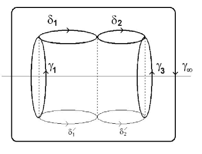
Figure 10: projection of the cycles $\gamma_{1},\gamma_{3},\gamma_{\infty},\delta_{1},\delta_{2}$ on the $x$-plane

Let $\kappa_{1}\in\pi_{1}(\mathcal{C},p_{1})$ be the loop shown on figure 11. The monodromy of the roots of the polynomial $f(x)$, induced by this loop are shown on fig. 12. Therefore, when $(a_{1},a_{2},a_{3})$ makes one turn along $\kappa$, the cycle $\gamma_{1}$ is transformed to $\gamma^{\prime}_{1}$, where

$$\gamma^{\prime}_{1}=\gamma_{1}+\delta_{1}-\delta^{\prime}_{1}=\gamma_{1}-\gamma_{3}+\gamma_{\infty}.$$

The monodromy of cycles is given by the following matrix (in the basis $\{\gamma_{1},\gamma_{3},\gamma_{\infty}\}$)

$$M_{\kappa_{1}}=\left(\begin{array}[]{ccc}1&0&0\\ -1&1&0\\ 1&0&1\\ \end{array}\right).$$

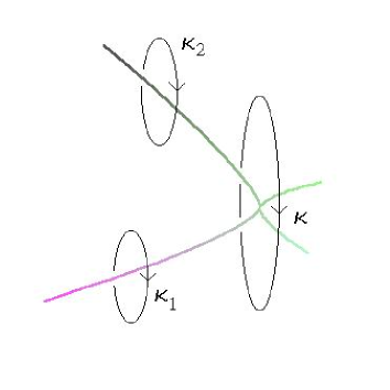
Figure 11: the loops $\kappa$

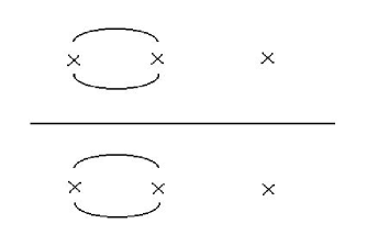
Figure 12: monodromy of the roots of $f(x)$

Consider the loop $\kappa_{2}\in\pi_{1}(\mathcal{C},p_{2})$ shown on figure 11. The monodromy of the roots of the polynomial $f(x)$ induced by $\kappa_{2}$ is shown on figure 13. The cycle $\gamma_{1}$ is transformed to $\gamma^{\prime}_{1}$ where

$$\gamma^{\prime}_{3}=\gamma_{3}+\delta_{2}-\delta^{\prime}_{2}=\gamma_{3}-\gamma_{1}+\gamma_{\infty}.$$

The monodromy of the cycles is given by the following matrix (in the basis $\{\gamma_{1},\gamma_{2},\gamma_{\infty}\}$)

$$M_{\kappa_{2}}=\left(\begin{array}[]{ccc}1&-1&0\\ 0&1&0\\ 0&1&1\\ \end{array}\right).$$

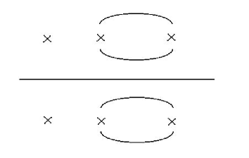
Figure 13: the monodromy of the roots of $f(x)$

In a similar way we may choose a third generator $\kappa_{3}$ and compute its image in $Aut(\mathbb{Z}^{3})$.

References

- [1] M. Adler-P. van Moerbeke, Linearization of Hamiltonian systems, Jacobi varieties and representation theory, Advances in Math., 38, p.318-379, (1980).
- [2] I.M.Aksenenkova, Vestnik Moskovskogo Universiteta, série 1, No 1, p.86-90, (1981), (Russian).
- [3] V.I. Arnold, Mathematical Methods of Classical Mechanics, Springer, (1978).
- [4] V.I.Arnold, S.M.Gusein-Zade, A.N.Varchenko, Singularities of Differentiable Maps, vol. 1 and II, Boston-Basel-Berlin (1988).
- [5] Bateman H.-Erdelyi A. Higher Transcendental Functions, Mc. Graw-Hill, New-York (1955).
- [6] L. Bates-M. Zou, Degeneration of Hamiltonian monodromy cycles, Nonlinearity, 6, p.313-335, (1993).
- [7] Larry M. Bates, Richard H. Cushman, Global aspects of classical integrable systems, Birkhäuser, 1997.
- [8] A. Beauville, Jacobiennes des courbes spectrales et systèmes Hamiltoniens complétement intégrales, Acta. Math., 164, p.211-235, (1990).
- [9] A.I. Bobenko-A.G. Reyman-M.A. Semenov-Tian-Shansky, The Kowalewski Top 99 Years Later : A Lax Pair, Generalzations and Explicit Solutions, Commun. Math. Phys., 122, p.312-354, (1989).
- [10] R. Cushman-H. Knörrer, The energy momentum mapping of Lagrange Top, Springer Lecture Notes in Mathematics, 1139, p.12-24, (1985).
- [11] R. Donagi-E. Markman, Spectral covers, algebraically completely integrable, Hamiltonian systems and moduli of bundles, Lectures Notes in Math., 1620, Springer, (1993).
- [12] J.J. Duistermaat, On Global Action Angles co-ordinates, Comm. Pure Appl. Math., 32, p.687-706, (1980).
- [13] J.-P. Françoise, Calculs explicites d’actions-angles, Séminaire de Mathématiques supérieures de l’Université de Montréal, 102, p.101-120, (1986).
- [14] J.-P. Françoise, Monodromy and the Kowalevskaya top, Astérisque ”Singularités d’Equations différentielles”, 150-151, p.87-108, (1987).
- [15] J.-P. Françoise, The Arnol’d Formula for A.C.I. systems, Bulletin of the American Mathematical Society, Vol 17, No 2,p.301-303, (1987).
- [16] L. Gavrilov, Generalized Jacobians of Spectral curves and completely integrable systems, Math. Z. 230 487-508 (1999).
- [17] L. Gavrilov, A. Zhivkov, The Complex Geometry of Lagrange Top, L’enseignement Mathématiques, t.44, p.133-170, (1998).
- [18] L. Gavrilov, O. Vivolo,The Real Period Function of Singularity and Perturbations of the Spherical Pendulum, Compositio Math. 119 2000.
- [19] C. Jacobi, Vorlesungen über Dynamik, G. Reimer, Berlin, (1891), Réimpression : Chelsea, New York, (1967).
- [20] S. Lang, Unramified class field theory over function fields in several variables, Ann. of Maths., 64, p.285-325, (1956).
- [21] S. Lang, Sur les séries L d’une variété algébrique, Bull. Soc. Math. de France, 84, p.385-407, (1956).
- [22] E. Looijenga, The Discriminant of a real simple singularity, Compositio Math., 37, p.51-62, (1978).
- [23] C. Médan, Thèse de Doctorat de l’Université Paul Sabatier, Toulouse, décembre 1997.
- [24] P. van Moerbeke-D. Mumford, The spectrum of difference operators and algebraic curves, Acta Math., 143, p.93-154, (1979).
- [25] D. Mumford, Tata Lectures on Theta II, Progress in Mathematics, vol 43, Birkhäuser, (1984).
- [26] T.Z. Nguyen, Symplectic topology of integrable Hamiltonian systems, Thèse Doctorat, Univ. Louis Pasteur, Strasbourg, (1994).
- [27] E. Previato, Hyperelliptic quasi-periodic and soliton solutions of the nonlinear Schrödinger equation, Duke Math. J. p.409-448, (1982).
- [28] T. Ratiu, P. van Moerbeke, The Lagrange rigid body motion, Ann. Inst. Fourier, Grenoble, 32, 1, p.211-234, (1982).
- [29] A.G. Reyman-M.A. Semenov-Tian-Shansky, Group theoretical methods in the theory of finite dimensional Integrable Systems, in Dynamical Systems VII, Encyclopedia of Mathematical Sciences, Springer, 16, (1994).
- [30] M. Rosenlicht, Generalized Jacobian varieties, Ann. of Maths, 59, p.505-530,(1954).
- [31] M. Rosenlicht, A universal mapping property of generalized Jacobian varieties, Ann. of Maths, 66, p.80-88, (1957).
- [32] J.P. Serre, Groupes Algébriques et Corps de Classes, Hermann, (1959).
- [33] R. Silhol, Real Abelian Varieties and the theory of Comessatti, Math. Z., 181, p.345-364, (1982).
- [34] O. Vivolo, Systèmes intégrables et courbes algébriques, PhD thesis, Université de Toulouse III, (1997).
- [35] O. Vivolo, The monodromy of action variables of Lagrange top, prépublication n 62, Université de Toulouse III, (1995).
- [36] E.T. Whittaker, A Treatise on the Analytical Dynamics of Particles and Bodies, Cambridge Univ. Press, (1904).
- [37] A. Weil, Euler and the Jacobians of elliptic curves, in Aritmetic and Geometry, Prog. Math. vol.35 (1983), Coats and Helgason (Eds), Birkhäuser.
- [38] A. Weil, Variétés abéliennes et courbes algébrique, Hermann, Paris, (1948).
- [39] M. Zou, Monodromy in two degrees of freedom integrable systems, in Journal of Geometry and Physics, 10, p.37-48, (1992).
- [40] M. Zou, Kolmogorov’s condition for the square potential spherical pendulum, Physics Letters A, 166, p.321-329, (1992).