Classifying Spinor Structures

Scott Morrison

The University of New South Wales

School of Mathematics

Department of Pure Mathematics

Scott Morrison

A thesis submitted for consideration in the degree of

Bachelor of Science with honours in pure mathematics at the

University of New South Wales.

June 2001

Supervisor: Dr. J. D. Steele

Acknowledgements

Firstly I would like to express my gratitude to John Steele, my supervisor, for his guidance and assistance, and for the considerable time he has invested in checking my drafts, clarifying my prose, and especially in trying to make my seminar make some sense!

A considerable number of members of the Mathematics Department have made available their time and mathematical expertise, or offered well considered academic advice over the past year.¹¹1In particular Prof. M. Cowling, Dr. S. Disney, Prof. T. Dooley and Dr. N. Wildberger, and outside the Department, Dr J. Baez, UCR, and Dr. J. Hillman, Sydney. Many thanks go for this, and also for the friendly academic environment of the Department, which has made working here a pleasure.

I would like to thank all my friends, who distracted me when I needed to be distracted, and allowed me to work when I needed to work. Finally, I would like to especially thank my family, without whose unfailing support this would never have been possible.

$\Delta\accentset{\smallfrown}{\iota}\nu o\varsigma\quad\beta\alpha\sigma\iota\lambda\epsilon\acute{\upsilon}\epsilon\iota\quad\tau\grave{o}\nu\quad\Delta\acute{\iota}^{\prime}\quad\accentset{\supset}{\epsilon}\xi\epsilon\lambda\eta\lambda\alpha\kappa\acute{\omega}\varsigma$

Spin has cast out Zeus and rules as king.²²2Aristophanes’ Clouds (l. 828). Aristophanes’ inspiration here is Anaxagoras, who held that ‘ $\delta\accentset{\smallfrown}{\iota}\nu o\varsigma$ ’, meaning ‘spin’ or ‘rotation’, was one of the primary effects of ‘ $\nu o\accentset{\smallfrown}{\upsilon}\varsigma$ ’, the active and rational principle of the Universe [35].

Introduction

The aim of this thesis is to investigate the mathematics of spinor structures, and their classification. The language of principal fibre bundles allows a thorough and coherent treatment of pseudo-Riemannian manifolds and spinor structures. The first two parts of this thesis give a fully geometric description of these constructions, including classification results for inequivalent spinor structures. The third part shows how the Dirac equation sits naturally in the setting of spinor structures, and how spinor structures allow us to generalise the Dirac equation to arbitrary curved space-times. It also discusses the implications in physics of the available choice of spinor structures. Although this interest in the Dirac equation guides the development of the material, we work in a more general setting. The mathematical focus is on the classification of spinor structures, and we consider the abstract setting both when reviewing previously known work and when presenting new work.

Fundamentally, there are two operations on principal fibre bundles which we are interested in. One is reducing the structure group. Such a reduction of the frame bundle picks out an orthonormal structure, and so gives an alternative treatment of pseudo-Riemannian manifolds. The details of this are given in Part I. We first show that pseudo-Riemannian metrics are in one to one correspondence with appropriate reductions of the frame bundle. Thereafter, we introduce the notion of a connection on a principal fibre bundle, and show that these give rise to the covariant derivatives familiar from pseudo-Riemannian geometry.

The other fundamental operation on principal fibre bundles is constructing the spinor bundle. This process ‘unwraps’ the structure group to its simply connected covering group. This is not always possible, and when possible, the spinor bundle need not be uniquely defined. In Part II, we give the relevant classifications in the general setting. This differs slightly from the more common notion of a spinor structure, which only considers two fold covering groups. We show how the general theory encompasses this case.

The combination of these two processes proves fruitful. The geometric description of pseudo-Riemannian geometry in terms of a reduction of the frame bundle given in Part I allows a beautifully geometric construction of the spinor structure, in §7.

To some extent the two processes are independent—for example, we prove that the classification of the possible spinor structures for Riemannian and Lorentzian manifolds is independent of the particular metric structure chosen, in §8. On the other hand, certain results are only available when we treat spinor structures of a reduced orthonormal bundle. In particular, the interplay allows a geometrical description of the calculus and algebra of spinor structures for pseudo-Riemannian manifolds. For example, in §9 we see that every spinor derivative, considered as a connection form on the spinor bundle, is simply the pull-back of the connection form on the original bundle. On a pseudo-Riemannian manifold there is a distinguished connection form, and so this construction picks out a distinguished connection on the spinor structure. In certain low dimensional cases, an exceptional isomorphism between the simply connected cover of the orthogonal group and another group, such as $SL(2,\mathbb{C})\cong\smash{\widetilde{SO}}_{0}(1,3)$ , allows an explicit development of the spinor algebra.

We also describe a coarse classification of spinor structures, according to the type of underlying principal fibre bundle, in §10. This classification extends previous work in this direction, and we see how it allows us to compare the spinor connections associated with different spinor structures.

All these ideas combine in Part III in the analysis of the Dirac equation. In four dimensional Minkowskian space-time the usual presentation of the Dirac equation, using ‘gamma matrices’, can be rewritten using the spinor algebra and calculus as a simple pair of covariant differential equations. This allows an immediate generalisation to curved Lorentzian space-times. Finally, we apply the classification of inequivalent spinor structures, and our knowledge of how the spinor connection depends on the choice of spinor structure, to consider the physical implications of the choice of spinor structure for particles governed by the Dirac equation.

Conventions used throughout

All our manifolds are considered to be Hausdorff, paracompact, and smooth. For these and other notions of topology and basic differential geometry, refer to [6] or the more abstract but more comprehensive exposition in [31, 32].

We use a subscripted asterisk to indicate the derivative of a function. Thus if $f:X\rightarrow Y$ is a smooth map, $f_{*}:TX\rightarrow TY$ , and at a point $x\in X$ , $f_{*x}:T_{x}X\rightarrow T_{f(x)}Y$ . Later we will also use this notation to indicate the induced map $f_{*}:\pi_{1}(X)\rightarrow\pi_{1}(Y)$ between the fundamental groups of $X$ and $Y$ , but it will always be clear from context which sense is intended.

We will write $K\preceq L$ to indicate that $K$ is a subgroup of $L$ .

If $G$ is a Lie group, $\mathfrak{G}$ denotes its Lie algebra. The Lie algebras of matrix groups will be denoted in the conventional manner. Thus, for example, $\mathfrak{so}(n)$ is the Lie algebra of the $n$ dimensional special orthogonal group $SO(n)$ . The adjoint representation of $G$ on $\mathfrak{G}$ is written $\operatorname{Ad}(g)$ , and defined as the derivative of the inner automorphism of $G$ , $g^{\prime}\mapsto I_{g}(g^{\prime})=gg^{\prime}g^{-1}$ , at the identity. Thus $\operatorname{Ad}(g)=I_{g*e}$ .

Part I Geometry of Orthonormal Structures

In the following sections, we review the theory of principal fibre bundles, and explain how pseudo-Riemannian geometry appears in this context. This has a dual purpose. Firstly, we wish to understand from an abstract point of view the nature of principal fibre bundles, because later, in Part II, this will be fundamental to understanding spinor structures. Secondly, spinor structures for pseudo-Riemannian manifolds are the most interesting variety of spinor structures, and so we need to place pseudo-Riemannian geometry in this framework.

The discussion of pseudo-Riemannian geometry consists of two main points. Firstly, every pseudo-Riemannian metric on a manifold corresponds to a certain reduction of the frame bundle of that manifold. Secondly, the covariant derivatives on such manifolds correspond exactly to connections on the reduced bundle. These facts are established in §4.3 and §5.4 respectively.

In the process of covering this material, we also give an introduction to the tensor algebra associated with a principal fibre bundle. This is useful in the proofs of this section, and will be vital in Part III in our discussion of the Dirac equation.

1. The theory of principal fibre bundles

We now give a brief introduction to the fundamental geometric objects underlying the rest of this work. These are principal fibre bundles. The definitions here follow [10], [27], [29] and [38]. A popular account of fibre bundles in physics appears in [5]. We first define a locally trivial fibre bundle.

1.1. Fibre bundles

A bundle $\xi=P\xrightarrow{\pi}M$ consists of a pair of smooth manifolds, $P$ and $M$ , respectively called the total space and the base space, and a surjective map $\pi:P\rightarrow M$ called the projection map.

A fibre bundle $\xi=P\xrightarrow{\pi}M$ with fibre $F$ is a bundle such that for each $m\in M$ , $\pi^{-1}(m)$ is diffeomorphic to $F$ . This partitioning of $P$ into $\bigcup_{m\in M}\pi^{-1}(m)$ is referred to as the fibration.

A fibre bundle morphism from a fibre bundle $\xi=P\xrightarrow{\pi}M$ with fibre $F$ to a fibre bundle $\eta=P^{\prime}\xrightarrow{\smash{\pi^{\prime}}}M^{\prime}$ with fibre $F^{\prime}$ is a pair of maps $(\phi,f)$ so $\phi:P\rightarrow P^{\prime}$ , $f:M\rightarrow M^{\prime}$ , and $\pi^{\prime}{\circ}\phi=f{\circ}\pi$ , such that the following diagram commutes.

This ensures that the maps respect the fibre structure.

Morphisms can be composed, as $(\phi^{\prime},f^{\prime}){\circ}(\phi,f)=(\phi^{\prime}{\circ}\phi,f^{\prime}{\circ}f)$ . If $M=M^{\prime}$ , we say $\xi$ and $\eta$ are $M$ -isomorphic, or equivalent, if there are morphisms $(\phi,f):\xi\rightarrow\eta$ , $(\phi^{\prime},f^{\prime}):\eta\rightarrow\xi$ so $(\phi^{\prime},f^{\prime}){\circ}(\phi,f)=(\operatorname{id}_{P},\operatorname{id}_{M})$ and $(\phi,f){\circ}(\phi^{\prime},f^{\prime})=(\operatorname{id}_{P^{\prime}},\operatorname{id}_{M})$ . The bundle $\xi$ is said to be trivial if it is $M$ -isomorphic to $M\times F\xrightarrow{\pi}M$ , the product fibre bundle. Henceforth we will nearly always consider only morphisms between bundles over the same base space, so $M=M^{\prime}$ , and $f=\operatorname{id}_{M}$ .

We can also restrict bundles. If $N$ is a submanifold of $M$ , define

\xi{}_{\mid N}{}=\pi^{-1}(N)\xrightarrow{\pi{}_{\mid\pi^{-1}(N)}{}}N.

With this idea, we can say that bundles $\xi$ and $\eta$ over $M$ are locally isomorphic if there is an open covering $\bigcup_{\alpha}U_{\alpha}$ of $M$ so for each $\alpha$ , $\xi{}_{\mid U_{\alpha}}{}$ and $\eta{}_{\mid U_{\alpha}}{}$ are ${U_{\alpha}}$ -isomorphic. We can now define locally trivial as meaning locally isomorphic to the product fibre bundle $M\times F$ . Each bundle morphism is of the form $\varphi:U\times F\rightarrow\pi^{-1}(U)$ , where $\pi(\varphi(m,f))=m$ for all $m\in U$ and $f\in F$ , and is called a local trivialisation of the fibre bundle. Generally no particular trivialisations are distinguished.

A section of a bundle is a smooth map $\sigma:M\rightarrow P$ such that $\pi{\circ}\sigma=\operatorname{id}_{M}$ . It assigns to each point $m\in M$ a point in the fibre of $m$ . A local section is simply a section defined only on some open set of $M$ .

1.2. Principal fibre bundles

We now reach the definition of a principal fibre bundle.

Definition 1.1.

A bundle $P\xrightarrow{\pi}M$ is a principal fibre bundle with structure group $G$ if

(1)

The group $G$ is a Lie group, and $G$ acts on the right on $P$ :

$\mathsf{p}\mapsto\mathsf{p}g.$
(2)

The $G$ action preserves the fibres of $P$ , and is transitive on fibres.
(3)

The $G$ action is free. That is, if $\mathsf{p}g=\mathsf{p}$ for some $\mathsf{p}\in P$ , then $g=e$ .
(4)

There are local trivialisations compatible with the $G$ action. That is, for each $m_{0}\in M$ , there is an open set $U$ with $m_{0}\in U\subset M$ and a map $\varphi:U\times G\rightarrow\pi^{-1}(U)$ so $\pi(\varphi(m,g))=m$ and $\varphi(m,g)=\varphi(m,e)g$ for all $m\in U$ and $g\in G$ .

It is clear from conditions 2. and 3. that the fibres of $P$ are diffeomorphic to $G$ . We write $G\rightsquigarrow P\xrightarrow{\smash[t]{\pi}}M$ to indicate this situation, where $G$ is the structure group acting on $P$ .

Condition 4. is in fact guaranteed if local trivialisations exist at all, in accordance with the following result.

Lemma 1.2.

If $P\xrightarrow{\pi}M$ is a bundle satisfying the first three parts of Definition 1.1, then there is a one to one correspondence between local sections $\sigma:U\rightarrow P$ on $U$ and local trivialisations $\varphi:U\times G\rightarrow\pi^{-1}(U)$ over $U$ compatible with the $G$ action.

Proof.

Clearly a local trivialisation (compatible with the $G$ action or not) defines a section, via $\sigma(m)=\varphi(m,e)$ . Given a section, define $\psi$ by $\psi(m,g)=\sigma(m)g$ . This is clearly compatible with the $G$ action. If we began with a trivialisation compatible wiht the $G$ action, these constructions are mutual inverses, establishing the correspondence. ∎

As the group $G$ acts transitively and freely on each fibre, if $\pi(\mathsf{p})=\pi(\mathsf{p^{\prime}})$ there is a unique $g\in G$ so $\mathsf{p}g=\mathsf{p^{\prime}}$ . We use this to define a function $\tau:\pi^{-1}(m)\times\pi^{-1}(m)\rightarrow G$ for each $m\in M$ , so $\mathsf{p}\tau(\mathsf{p},\mathsf{p^{\prime}})=\mathsf{p^{\prime}}$ . We call this the translation function for the principal fibre bundle.

A principal fibre bundle morphism is a fibre bundle morphism that commutes with the group action. Thus if $G\rightsquigarrow P\xrightarrow{\smash[t]{\pi}}M$ and $G\rightsquigarrow P^{\prime}\xrightarrow{\smash[t]{\pi^{\prime}}}M$ are principal fibre bundles, then a smooth map $u:P\rightarrow P^{\prime}$ is a principal fibre bundle morphism if $\pi^{\prime}{\circ}u=\pi$ and $u(\mathsf{p}g)=u(\mathsf{p})g$ for all $\mathsf{p}\in P$ and $g\in G$ .

It turns out that for any fibre bundle there is a related principal fibre bundle, where, roughly speaking, the structure group is the group of transformations of the fibre [29, §3.3]. Any fibre bundle can then be derived from its principal fibre bundle by the associated bundle construction. This is given for vector space fibres in §2.2, and it is used subsequently to construct the tensor algebra associated with a representation of the structure group of a principal fibre bundle.

1.3. An example: the frame bundle of a manifold

The primary motivating example of a principal fibre bundle is the frame bundle of a manifold. Given a smooth $n$ dimensional manifold $M$ , at each point $m$ the tangent space $T_{m}M$ is defined as the vector space of tangent vectors³³3Tangent vectors are in turn defined as derivations of the germs of smooth functions, although we shall not need this. at that point. The collection of all the tangent spaces is called the tangent bundle, and denoted $TM$ . A frame is simply a basis for the tangent space at a point. We might write a frame as $\mathsf{p}=(e_{1},\ldots,e_{n})$ , where the $e_{i}$ are tangent vectors. The frame bundle, as a set, is the collection of frames at every point of the manifold. We denote the frame bundle of $M$ by $FM$ . It has a projection $\pi$ taking a frame to the point at which that frame lies. We give it a smooth structure as an $n^{2}+n$ dimensional manifold in the obvious way.⁴⁴4We induce the smooth structure for the frame bundle from the smooth structure for the manifold itself. A coordinate chart $\varphi:U\rightarrow V$ , where $U\subset M$ , and $V\subset\mathbb{R}^{n}$ are open sets, induces a map $\varphi_{*}:FU\rightarrow FV$ by $\varphi_{*}(e_{1},\ldots,e_{n})=(\varphi_{*}e_{1},\ldots\varphi_{*}e_{n})$ . That is, $\varphi$ pushes forward a frame on $M$ to a frame on $\mathbb{R}^{n}$ . Now, the frame bundle of $\mathbb{R}^{n}$ , $F\mathbb{R}^{n}$ has an obvious smooth structure, since the tangent space to $\mathbb{R}^{n}$ is canonically identified with $\mathbb{R}^{n}$ . Thus $FV\cong V\times\mathbb{R}^{n^{2}}$ , and if we say that $\varphi_{*}:FU\rightarrow V\times\mathbb{R}^{n^{2}}$ is a chart, for each coordinate chart $\varphi$ , we obtain an atlas for $FM$ , and so a smooth structure.

Next we see that $FM$ really is a principal fibre bundle. To do this, we must describe the group action. The general linear group $GL(n,\mathbb{R})$ acts on the right on frames in the following way. If $g\in GL(n,\mathbb{R})$ , and $\mathsf{p}=(e_{1},\ldots,e_{n})\in FM$ , then we have

\displaystyle g

\displaystyle=\begin{pmatrix}g^{1}{}_{1}&\cdots&g^{1}{}_{n}\\ \vdots&\ddots&\vdots\\ g^{n}{}_{1}&\cdots&g^{n}{}_{n}\end{pmatrix}

and

\displaystyle\mathsf{p}g

\displaystyle=(e_{1},\ldots,e_{n})\begin{pmatrix}g^{1}{}_{1}&\cdots&g^{1}{}_{n}\\ \vdots&\ddots&\vdots\\ g^{n}{}_{1}&\cdots&g^{n}{}_{n}\end{pmatrix}.

(1.1)

We can now check that the principal fibre bundle axioms from Definition 1.1 are satisfied. All are in fact immediately obvious, except perhaps the existence of local trivialisations, which are provided by the coordinate charts of $M$ .

Throughout later discussions, in which we discuss theorems dealing with abstract principal fibre bundles, it may be useful to keep in mind this concrete and intuitive example.

2. Tensor algebras

We now begin our discussion of tensors. Our aim is to define the global tensor algebra associated with a $G$ principal fibre bundle and a representation of the group $G$ . We will also present a powerful formalism for calculations in the global tensor algebra, called the abstract index notation. We will use this throughout our discussion of covariant differentiation and tensor calculus in §5, and eventually in the exposition of the Dirac equation in §14. It is worth asking why we decide to present this material in the completely general setting, allowing an arbitrary (finite dimensional) representation of an arbitrary Lie group. Later, we treat in detail two tensor algebras, one associated with the group $GL(n,\mathbb{R})$ , and the other associated with $SL(2,\mathbb{C})$ . Having the general framework available avoids unnecessary duplication.

To start, we need to describe the local tensor algebra associated with a representation $\lambda$ of a Lie group $G$ . This is straightforward and familiar. Although the abstract index notation is irrelevant for local tensor algebras, we introduce it in this context in order to streamline the development of the global tensor algebra.

Following this, we construct the global tensor algebra. The data required are a local tensor algebra based upon a representation $\lambda$ of a Lie group $G$ , and a principal fibre bundle $G\rightsquigarrow P\xrightarrow{\smash[t]{\pi}}M$ , with structure group $G$ , over a manifold $M$ . Using the associated vector bundle construction, given below in §2.2, we define tensors on the base manifold. In the particular case of the $GL(n,\mathbb{R})$ frame bundle over a manifold, this process gives the world tensor algebra, in terms of the tangent vectors to the manifold.

2.1. Local tensor algebras

To begin, we introduce the most primitive type of tensor algebra. It is a local tensor algebra in the sense that there is a singled fixed underlying representation on a fixed vector space. The purpose of this section is not only to define tensors—which, it is hoped, will be fairly familiar in any case—but to describe the abstract index tensor algebra, and distinguish between the objects of this algebra and the underlying geometrical objects.

We first introduce the geometric tensor algebra. To this end, suppose $G$ is an arbitrary Lie group. Suppose $\lambda$ is a representation of $G$ on the $n$ dimensional vector space $V=\mathbb{F}^{n}$ over the field $\mathbb{F}=\mathbb{R}$ or $\mathbb{C}$ . A typical example might be the matrix representation of $GL(n,\mathbb{R})$ acting on $\mathbb{R}^{n}$ with the standard basis. The elements of $V$ are geometrical objects. We might denote such an element by $v$ . Since we have fixed a basis, we can consider the components of $v$ , writing these as the kernel symbol along with a numerical superscript index, $v^{1},\ldots,v^{n}\in\mathbb{F}$ .

Next, we consider the dual vector space $V^{*}$ , which is canonically isomorphic to $\mathbb{F}^{n}$ also, since we have selected a basis for $V$ . Specific components of $u\in V^{*}$ are indicated with numerical indices, as in $u_{1},\ldots,u_{n}\in\mathbb{F}$ .

The pairing between the vector space and its dual, $V^{*}\times V\rightarrow\mathbb{F}$ is written $(u,v)\mapsto\{u,v\}$ . In terms of components, this is

\{u,v\}=\sum_{k=1}^{n}u_{k}v^{k}.

The representation $\lambda$ on $V$ gives rise to the dual representation $\lambda^{*}$ on $V^{*}$ , defined so

\{(\lambda^{*}(g)u),v\}=\{u,(\lambda(g^{-1})v)\}

(2.1)

for all $u\in V^{*}$ and $v\in V$ .

With these two fundamental representations established, we generate all the tensor representations. The underlying vector space for the valence $\left[\begin{smallmatrix}k\\ l\end{smallmatrix}\right]$ tensor representation is the collection of multilinear maps

\underbrace{V^{*}\times\dots\times V^{*}}_{k\text{ times}}\times\underbrace{V\times\dots\times V}_{l\text{ times}}\rightarrow\mathbb{F}.

We denote this vector space as $\mathcal{T}\!\begin{smallmatrix}k\\ l\end{smallmatrix}$ . In particular $V=\mathcal{T}\!\begin{smallmatrix}1\\ 0\end{smallmatrix}$ and $V^{*}=\mathcal{T}\!\begin{smallmatrix}0\\ 1\end{smallmatrix}$ . The action of $G$ on the vector space $\mathcal{T}\!\begin{smallmatrix}k\\ l\end{smallmatrix}$ is such that for $S\in\mathcal{T}\!\begin{smallmatrix}k\\ l\end{smallmatrix}$ ,

(g(S))(x^{1},\ldots,x^{k},y_{1},\ldots,y_{l})=\\ =S(\lambda^{*}(g^{-1})x^{1},\ldots,\lambda^{*}(g^{-1})x^{k},\lambda(g^{-1})y_{1},\ldots,\lambda(g^{-1})y_{l}),

where $x^{1},\ldots,x^{k}\in V^{*}$ and $y_{1},\ldots y_{l}\in V$ . This defines a representation of $G$ on $\mathcal{T}\!\begin{smallmatrix}k\\ l\end{smallmatrix}$ .

We now outline three operations on tensors. Firstly, we can take the tensor product of two tensors. This is a map $\mathcal{T}\!\begin{smallmatrix}j\\ k\end{smallmatrix}\times\mathcal{T}\!\begin{smallmatrix}l\\ m\end{smallmatrix}\rightarrow\mathcal{T}\!\begin{smallmatrix}j+l\\ k+m\end{smallmatrix}$ . The tensor product of $S\in\mathcal{T}\!\begin{smallmatrix}j\\ k\end{smallmatrix}$ and $T\in\mathcal{T}\!\begin{smallmatrix}l\\ m\end{smallmatrix}$ is defined by

(S\otimes T)(x^{1},\ldots,x^{j},x^{j+1},\ldots,x^{j+l},y_{1},\ldots,y_{k},y_{k+1},\ldots,y_{k+m})=\\ =S(x^{1}\ldots,x^{j},y_{1},\ldots,y_{k})T(x^{j+1},\ldots,x^{j+l},y_{k+1},\ldots,y_{k+m}),

where $x^{1},\ldots,x^{j+l}\in V^{*}$ , and $y_{1},\ldots,y_{k+m}\in V$ . Further, it is easy to see that this map intertwines the representations.

Secondly, we can perform ‘index permutation’. This name will become clearer later. Given a tensor $S$ in $\mathcal{T}\!\begin{smallmatrix}k\\ l\end{smallmatrix}$ , we can obtain $k!l!$ new tensors in $\mathcal{T}\!\begin{smallmatrix}k\\ l\end{smallmatrix}$ , all of which will in general be different, by permuting its arguments. For example, if $S\in\mathcal{T}\!\begin{smallmatrix}2\\ 0\end{smallmatrix}$ , then there is another tensor, which we might call for a moment $\widetilde{S}$ in $\mathcal{T}\!\begin{smallmatrix}2\\ 0\end{smallmatrix}$ , given by $\widetilde{S}(w,z)=S(z,w)$ , for all $w,z\in V^{*}$ . Again, it is easy to see that this operation commutes with the action of $G$ via the tensor representation, and so the index permutation maps intertwine the $\mathcal{T}\!\begin{smallmatrix}k\\ l\end{smallmatrix}$ representation with itself.

Finally, we can contract a tensor. Given an tensor $S$ in $\mathcal{T}\!\begin{smallmatrix}k\\ l\end{smallmatrix}$ , this produces a tensor in $\mathcal{T}\!\begin{smallmatrix}k-1\\ l-1\end{smallmatrix}$ , which we for the moment call $\hat{S}$ , which acts as

\hat{S}(x^{1},\ldots x^{k-1},y_{1},\ldots,y_{l-1})=\sum_{i=1}^{n}T(x^{1},\ldots x^{k-1},e^{i},y_{1},\ldots,y_{l-1},e_{i}),

where $x^{1},\ldots,x^{k-1}\in V^{*}$ and $y_{1},\ldots y_{l-1}\in V$ , and $e^{i}$ and $e_{i}$ are the basis vectors for $V^{*}$ and $V$ respectively. We lose no generality by only discussing contraction over the last argument, because by combining this operation with index permutation, we can contract with respect to any pair of arguments, one in $V$ , the other in $V^{*}$ . Contraction also commutes with the action of $G$ . However, we will not prove this now, as it is more transparent in index notation.

These comments complete our description of the geometric tensor algebra, in that we have specified the objects and algebra operations. This presentation is, however, rather unsatisfactory for working with these tensors, because its notation is so cumbersome. Firstly, we cannot see from the symbol for an element of the tensor algebra which representation it lies in, and the operations of permutation and contraction require specialised notation for each possible pair of indices involved.

Thus, we now introduce the abstract index tensor algebra. At first it seems more mathematically cumbersome, but it has great notational convenience. When we come to global tensor algebras, the abstract index notation offers a powerful formalism without reference to local coordinates or components. The principal difference between abstract index notation and conventional tensor index notation is that objects indicated, for example, as $V^{\mathfrak{a}}{}_{\mathfrak{bc}}$ do not denote the components of a tensor, but the tensor itself, with the indices serving as labels to indicate the valence. A further useful discussion on the motivation for abstract index notation is in [53, pp. 23–26]. The idea of abstract index tensors is due to Penrose, and they are described in his works [46, 47]. A thorough axiomatic development is given in [47, pp. 76–91], and a simple presentation of the formalism is in [46, §3].

We now give an explicit description of the abstract index algebra and its operations. We introduce an index set, denoted $\mathcal{L}$ . For our purposes now, it will be $\mathcal{L}=\left\{\mathfrak{a},\mathfrak{b},\mathfrak{c},\ldots,\mathfrak{a}_{1},\mathfrak{b}_{1},\dots,\mathfrak{a}_{2},\ldots\right\}$ . The gothic font will be used in the index set when we are referring to the tensor algebra associated to some arbitrary group. Later, we will use lowercase or uppercase Roman indices to refer specifically to the tensors associated to the groups $GL(n,\mathbb{R})$ and $SL(2,\mathbb{C})$ respectively. The labels in the index set at this point are all lightface, to emphasise that this is a local tensor algebra. Later, global tensor algebras will use boldface indices. The elements of the abstract index algebra are pairs, the first part of which is an element from the geometric tensor algebra, while the second part is an appropriate sequence of indices from $\mathcal{L}$ . For a tensor $S$ in $\mathcal{T}\!\begin{smallmatrix}k\\ l\end{smallmatrix}$ , this is a sequence of $k+l$ distinct indices from $\mathcal{L}$ . We never write this pair explicitly as $(S,\{\mathfrak{a}_{1},\ldots,\mathfrak{a}_{k},\mathfrak{b}_{1},\ldots,\mathfrak{b}_{l}\})$ , but as

S^{\mathfrak{a}_{1}\dots\mathfrak{a}_{k}}{}_{\mathfrak{b}_{1}\dots\mathfrak{b}_{l}}.

Thus corresponding to each geometrical object in the tensor algebra, there are a collection of objects in the abstract index algebra. We write $\mathcal{T}^{\mathfrak{a}_{1}\dots\mathfrak{a}_{k}}{}_{\mathfrak{b}_{1}\dots\mathfrak{b}_{l}}$ for the vector space of elements of the abstract index tensor algebra of the form $S^{\mathfrak{a}_{1}\dots\mathfrak{a}_{k}}{}_{\mathfrak{b}_{1}\dots\mathfrak{b}_{l}}$ for some $S\in\mathcal{T}\!\begin{smallmatrix}k\\ l\end{smallmatrix}$ .

Example.

If $v\in V$ is a vector, then there are elements $v^{\mathfrak{a}},v^{\mathfrak{b}},v^{\mathfrak{c}}$ and so on in the abstract index algebra. The elements $v^{\mathfrak{a}}$ and $v^{\mathfrak{b}}$ correspond to the same geometrical object, $v$ , but are not equal in the abstract index tensor algebra. Similarly, a tensor $S\in\mathcal{T}\!\begin{smallmatrix}2\\ 0\end{smallmatrix}$ has representatives $S^{\mathfrak{ab}}$ , $S^{\mathfrak{ef}}$ , etc.

Next, we describe the tensor algebra operations in terms of abstract index notation. The tensor product appears as a map

\mathcal{T}^{\mathfrak{a}_{1}\dots\mathfrak{a}_{j}}{}_{\mathfrak{b}_{1}\dots\mathfrak{b}_{k}}\times\mathcal{T}^{\mathfrak{c}_{1}\dots\mathfrak{c}_{l}}{}_{\mathfrak{d}_{1}\dots\mathfrak{d}_{m}}\rightarrow\mathcal{T}^{\mathfrak{a}_{1}\dots\mathfrak{a}_{j}\mathfrak{c}_{1}\dots\mathfrak{c}_{l}}{}_{\mathfrak{b}_{1}\dots\mathfrak{b}_{k}\mathfrak{d}_{1}\dots\mathfrak{d}_{m}}.

All of the indices appearing as labels of the above vector spaces must be distinct. For example, the tensor product of $s^{\mathfrak{a}}$ and $t^{\mathfrak{b}}$ is an element of $\mathcal{T}^{\mathfrak{ab}}$ , written simply as $s^{\mathfrak{a}}t^{\mathfrak{b}}$ . The corresponding geometric tensor is the map $(w,z)\mapsto\{w,s\}\{z,t\}$ , for $w$ and $z$ in $V^{*}$ . In the abstract index formulation the tensor product is in fact commutative, because we define $t^{\mathfrak{b}}s^{\mathfrak{a}}\in\mathcal{T}^{\mathfrak{ab}}$ to correspond to exactly the same underlying geometric tensor. The indices indicate the order of arguments. On the other hand $t^{\mathfrak{a}}s^{\mathfrak{b}}\in\mathcal{T}^{\mathfrak{ab}}$ corresponds to a different geometric tensor, $(w,z)\mapsto\{w,t\}\{z,s\}$ . Index permutation has a simple appearance now, and the name becomes clear. If, for example $S^{\mathfrak{ab}}\in\mathcal{T}^{\mathfrak{ab}}$ , then $S^{\mathfrak{ba}}$ is the element of $\mathcal{T}^{\mathfrak{ab}}$ (not $\mathcal{T}^{\mathfrak{ba}}$ —but this will always be clear from context) corresponding to the tensor $(w,z)\mapsto S(z,w)$ for $w$ and $z$ in $V^{*}$ . Thus the operation of permuting arguments is indicated clearly by permuting the indices of the abstract index tensor. We must be careful however only ever to permute superscript indices, or to permute subscript indices. Finally, contraction is indicated by a repeated index, one superscript, one subscript. Thus $S^{\mathfrak{a}_{1}\dots\mathfrak{a}_{k-1}\mathfrak{c}}{}_{\mathfrak{b}_{1}\dots\mathfrak{b}_{l-1}\mathfrak{c}}$ is the element of $\mathcal{T}^{\mathfrak{a}_{1}\dots\mathfrak{a}_{k-1}}{}_{\mathfrak{b}_{1}\dots\mathfrak{b}_{l-1}}$ which corresponds to the contraction of $S\in\mathcal{T}\!\begin{smallmatrix}k\\ l\end{smallmatrix}$ . Contraction on other pairs of indices is defined similarly, by contraction of the underlying geometric tensor on the corresponding pair of arguments.

Because each of the tensor algebra operations is defined in terms of operations on the underlying geometric tensors, an equation between abstract index tensors remains true if one index is replaced throughout the equation by a new one.

Now, $\lambda(g)$ maps $V$ to $V$ , and is thus equivalently a map of $V^{*}\times V$ to $\mathbb{F}$ . Then $\lambda(g)$ is a valence $\left[\begin{smallmatrix}1\\ 1\end{smallmatrix}\right]$ tensor, and we denote it in abstract index notation as $g^{\mathfrak{a}}{}_{\mathfrak{b}}$ . Recall that since we are working over a fixed vector space, we can also consider the actual components of a tensor. The numbers $g^{1}{}_{1},g^{2}{}_{1}$ and so on are exactly the entries of the matrix $g$ . The action of the representation can now be written out. In the tensor algebra $\lambda(g)v$ corresponds to $g^{\mathfrak{a}}{}_{\mathfrak{b}}v^{\mathfrak{b}}$ in $\mathcal{T}^{\mathfrak{a}}$ . Since $\lambda$ is a representation, $(gh)^{\mathfrak{a}}{}_{\mathfrak{b}}=g^{\mathfrak{a}}{}_{\mathfrak{c}}h^{\mathfrak{c}}{}_{\mathfrak{b}}$ . Similarly the dual representation is simply written in index notation. According to Equation (2.1),

	$\displaystyle(\lambda^{*}(g)u)_{\mathfrak{b}}v^{\mathfrak{b}}$	$\displaystyle=\{\lambda^{*}(g)u,v\}$
		$\displaystyle=\{u,\lambda(g^{-1})v\}$
		$\displaystyle=u_{\mathfrak{a}}(\lambda(g^{-1})v)^{\mathfrak{a}}$
		$\displaystyle=u_{\mathfrak{a}}(g^{-1})^{\mathfrak{a}}{}_{\mathfrak{b}}v^{\mathfrak{b}},$

and so $\lambda^{*}(g)u$ corresponds to $(g^{-1})^{\mathfrak{a}}{}_{\mathfrak{b}}u_{\mathfrak{a}}$ in $\mathcal{T}_{\mathfrak{b}}$ . We use these expressions for the representations to express the action of $G$ in the tensor representation on $\mathcal{T}\!\begin{smallmatrix}k\\ l\end{smallmatrix}$ . An element $g\in G$ acting on a tensor $S$ in the $\left[\begin{smallmatrix}k\\ l\end{smallmatrix}\right]$ tensor representation gives a valence $\left[\begin{smallmatrix}k\\ l\end{smallmatrix}\right]$ tensor which in abstract index notation is

g^{\mathfrak{a}_{1}}{}_{\mathfrak{c}_{1}}\dotsm g^{\mathfrak{a}_{k}}{}_{\mathfrak{c}_{k}}(g^{-1})^{\mathfrak{d}_{1}}{}_{\mathfrak{b}_{1}}\dotsm(g^{-1})^{\mathfrak{d}_{l}}{}_{\mathfrak{b}_{l}}S^{\mathfrak{c}_{1}\dots\mathfrak{c}_{k}}{}_{\mathfrak{d}_{1}\dots\mathfrak{d}_{l}}.

(2.2)

It is straightforward to check that this is in fact a representation, using $(gh)^{\mathfrak{a}}{}_{\mathfrak{b}}=g^{\mathfrak{a}}{}_{\mathfrak{c}}h^{\mathfrak{c}}{}_{\mathfrak{b}}$ .

Finally, we use the abstract index presentation of the representations to show that contraction commutes with the group action. A simple case suffices, so we avoid a profusion of indices. Suppose $S^{a}{}_{b}\in\mathcal{T}^{a}{}_{b}$ . Then $g\in G$ acts on $S$ to give $(g)^{a}{}_{c}(g^{-1})^{d}{}_{b}S^{c}{}_{d}$ . Contracting on the indices $a$ and $b$ , we obtain

	$\displaystyle(g)^{a}{}_{c}(g^{-1})^{d}{}_{b}S^{c}{}_{d}$	$\displaystyle=(g^{-1}g)^{d}{}_{c}S^{c}{}_{d}$
		$\displaystyle=(e)^{d}{}_{c}S^{c}{}_{d}$
		$\displaystyle=S^{d}{}_{d}.$

This is exactly the result we would obtain contracting first and then acting by $g$ . The general case, with arbitrarily many indices, is much the same.

2.2. Associated vector bundles

Fundamental to the idea of a global tensor algebra is the notion of an associated vector bundle, which we will develop here, following [29, §3.3]. Say $G\rightsquigarrow P\xrightarrow{\smash[t]{\pi}}M$ is a principal fibre bundle, and $\lambda$ is a finite dimension representation of the group $G$ on a vector space $V$ . We will write this action of $G$ on $V$ as $(g,v)\mapsto\lambda(g)v$ for $g\in G$ and $v\in V$ . We consider the product space $P\times V$ . Define on this an equivalence relation $\sim$ , so that

(\mathsf{p},v)\sim(\mathsf{p}g,\lambda(g^{-1})v)

or equivalently

(\mathsf{p}g,v)\sim(\mathsf{p},\lambda(g)v).

We call the set of equivalence classes $(P\times V)/\sim$ the associated vector bundle for $\lambda$ . The vector bundle is also denoted as $P\times_{G}V$ . It is given the quotient topology, and so in particular if $\mathsf{p}_{\alpha}\xrightarrow{\alpha}\mathsf{p}$ and $v_{\alpha}\xrightarrow{\alpha}v$ , then $[\mathsf{p}_{\alpha},v_{\alpha}]\xrightarrow{\alpha}[\mathsf{p},v]$ .⁵⁵5A smooth structure is determined as follows. Given a coordinate chart $\phi:U\subset M\rightarrow\mathbb{R}^{p}$ , and a local section $\sigma:U\rightarrow P$ , define $\psi:\pi^{-1}(U)\times_{G}V$ by $\psi([\sigma(m),v])=(\phi(m),v)$ . The collection of all of these provide an atlas for $P\times_{G}V$ .

Such a vector bundle is clearly a fibre bundle, with fibre $V$ , and locally trivialisable. Since the fibre is the vector space $V$ , we can perform the usual vector space operations on elements of the vector bundle lying over the same point of the base manifold. Suppose for example that $\mathsf{p},\mathsf{p^{\prime}}\in P$ , $\pi(\mathsf{p})=\pi(\mathsf{p^{\prime}})$ , and $\mathsf{p^{\prime}}=\mathsf{p}g$ for some $g\in G$ . Then $[\mathsf{p},v]+[\mathsf{p^{\prime}},u]=[\mathsf{p},v+\lambda(g)u]$ .

2.3. General construction of a global tensor algebra

Equipped with this construction, we can describe the global abstract index tensor algebra associated with a principal fibre bundle and a particular representation of the structure group. Firstly, we construct the local abstract index tensor algebra, which is generated by the representation, as in §2.1. The global tensor algebra then arises as a collection of associated bundles. Conventional developments differ in that they emphasise the algebraic properties of the global tensor algebra, and consider it central. On the other hand, we consider the principal fibre bundle as primary, and the global tensor algebra as secondary.

For each abstract index tensor representation $\mathcal{T}^{\mathfrak{a}_{1}\dots\mathfrak{a}_{k}}{}_{\mathfrak{b}_{1}\dots\mathfrak{b}_{l}}$ , define the associated vector bundle

\mathcal{T}^{\boldsymbol{\boldsymbol{\mathfrak{a}}}_{1}\dots\boldsymbol{\boldsymbol{\mathfrak{a}}}_{k}}{}_{\boldsymbol{\boldsymbol{\mathfrak{b}}}_{1}\dots\boldsymbol{\boldsymbol{\mathfrak{b}}}_{l}}=P\times_{G}\mathcal{T}^{\mathfrak{a}_{1}\dots\mathfrak{a}_{k}}{}_{\mathfrak{b}_{1}\dots\mathfrak{b}_{l}}.

Thus a typical element of $\mathcal{T}^{\boldsymbol{\boldsymbol{\mathfrak{a}}}_{1}\dots\boldsymbol{\boldsymbol{\mathfrak{a}}}_{k}}{}_{\boldsymbol{\boldsymbol{\mathfrak{b}}}_{1}\dots\boldsymbol{\boldsymbol{\mathfrak{b}}}_{l}}$ is

S^{\boldsymbol{\boldsymbol{\mathfrak{a}}}_{1}\dots\boldsymbol{\boldsymbol{\mathfrak{a}}}_{k}}{}_{\boldsymbol{\boldsymbol{\mathfrak{b}}}_{1}\dots\boldsymbol{\boldsymbol{\mathfrak{b}}}_{l}}=[\mathsf{p},S^{\mathfrak{a}_{1}\dots\mathfrak{a}_{k}}{}_{\mathfrak{b}_{1}\dots\mathfrak{b}_{l}}]

for some $S\in\mathcal{T}\!\begin{smallmatrix}k\\ l\end{smallmatrix}$ . These objects are the global tensors, and take indices from the same labelling set as the local tensor algebra, but with boldface indices, to distinguish them from the local tensors. Such a tensor is only defined at a single point, the point $\pi(\mathsf{p})\in M$ —a tensor field is a cross section of this associated bundle.

Combining in this fashion the notational convenience of the local abstract index algebra and the geometric construction of an associated vector bundle, we obtain an extremely useful description of the tensors on a manifold. The tensor operations of forming tensor products, performing index permutations, and taking contractions, all have simple presentations. Specifically, to perform any of these operations on elements of the global tensor algebra, we simply perform the operation on the corresponding element of the local tensor algebra. As we have seen, the tensor operations in the local tensor algebra all commute with the group action, ensuring that this prescription for the tensor operations in the global tensor algebra is well defined.

Example.

Suppose $S_{\boldsymbol{\boldsymbol{\mathfrak{ab}}}}=[\mathsf{p},S_{\mathfrak{ab}}]$ and $y^{\boldsymbol{\boldsymbol{\mathfrak{c}}}}=[\mathsf{p^{\prime}},y^{\mathfrak{c}}]$ . Then there is some $g\in G$ so $\mathsf{p^{\prime}}=\mathsf{p}g$ , and we can define $x^{\mathfrak{c}}$ by $x^{\mathfrak{c}}=g^{\mathfrak{c}}{}_{\mathfrak{d}}y^{\mathfrak{d}}$ , so $y^{\boldsymbol{\boldsymbol{\mathfrak{c}}}}=[\mathsf{p},x^{\mathfrak{c}}]$ . In this case, we give examples of tensor operations. In each case the expression on the left is defined by that on the right.

	$\displaystyle S_{\boldsymbol{\boldsymbol{\mathfrak{ba}}}}$	$\displaystyle=[\mathsf{p},S_{\mathfrak{ba}}],$
	$\displaystyle S_{\boldsymbol{\boldsymbol{\mathfrak{ab}}}}y^{\boldsymbol{\boldsymbol{\mathfrak{c}}}}$	$\displaystyle=[\mathsf{p},S_{\mathfrak{ab}}x^{\mathfrak{c}}],$
and
	$\displaystyle S_{\boldsymbol{\boldsymbol{\mathfrak{ab}}}}y^{\boldsymbol{\boldsymbol{\mathfrak{b}}}}$	$\displaystyle=[\mathsf{p},S_{\mathfrak{ab}}x^{\mathfrak{b}}].$

2.4. World tensors

We now specialise this machinery to deal with the world tensors—that is, tensors defined in terms of tangent vectors to a manifold. The tangent bundle has a direct and geometrical interpretation, and need not be described as a vector bundle associated to a principal fibre bundle, in this case the $GL(n,\mathbb{R})$ frame bundle. However, when we later come to define spinors, there is no analogous direct interpretation. They must be constructed geometrically as an associated vector bundle. Preempting this, we show how that tangent bundle, and its related tensor bundles, are generated from the frame bundle, applying the theory of local tensor algebras and associated vector bundles.

The relevant Lie group is $GL(n,\mathbb{R})$ , acting on $\mathbb{R}^{n}$ . As in §2.1, there is an abstract index local tensor algebra. The index set will consist of lowercase Roman letters. The relevant principal fibre bundle is the frame bundle described in §1.3.

We can now reobtain the tangent bundle, as an associated vector bundle. Specifically, $TM\cong FM\times_{GL(n,\mathbb{R})}\mathbb{R}^{n}$ , as follows. If $\mathsf{p}=(e_{1},\ldots,e_{n})\in FM$ , and $v\in\mathbb{R}^{n}$ , then

[\mathsf{p},v]=\sum_{i=1}^{n}e_{i}v^{i}=(e_{1},\ldots,e_{n})\begin{pmatrix}v^{1}\\ \vdots\\ v^{n}\end{pmatrix}.

This is well defined, as

\displaystyle[\mathsf{p}g,v]=(e_{1},\ldots,e_{n})\begin{pmatrix}g^{1}{}_{1}&\cdots&g^{1}{}_{n}\\ \vdots&\ddots&\vdots\\ g^{n}{}_{1}&\cdots&g^{n}{}_{n}\end{pmatrix}\begin{pmatrix}v^{1}\\ \vdots\\ v^{n}\end{pmatrix}=[\mathsf{p},gv].

Equipped with this isomorphism, we henceforth always consider the frame bundle as primary, and the tangent bundle a derived object.

Producing the world tensor algebra is now simply a matter of stating that it is the global abstract index algebra associated with the frame bundle, and the representation of $GL(n,\mathbb{R})$ on $\mathbb{R}^{n}$ . Thus for example we have tensor bundles $\mathcal{T}^{\boldsymbol{\boldsymbol{ab}}}{}_{\boldsymbol{\boldsymbol{cd}}}$ , etc. Tensor operations all have a simple appearance in abstract index notation, but we are assured that no reference is made to local coordinates or components. That is, abstract index tensor equations are true equations between tensors.

2.5. Product bundles

Later, we will deal with two principal fibre bundles at once, with one generally the frame bundle. In this case, we can have vectors and tensors associated with either the frame bundle or the abstract principal fibre bundle. If we wish to emphasis that tensors are associated to the frame bundle, we call them world tensors, as above. Tensors associated to a principal fibre bundle other than the frame bundle will use special indices, either a gothic script for an abstract principal fibre bundle, or uppercase Roman characters for an $SL(2,\mathbb{C})$ spinor structure, defined later. Often, especially when using covariant derivatives in §5.3, we will need tensors with indices associated with both of the bundles. This can be formalised by considering these tensors as tensors in a vector bundle associated to the product bundle, which we mention now.

Definition (Product bundle over a base space).

Suppose

\xi=G\rightsquigarrow P\xrightarrow{\smash[t]{\pi_{P}}}M\textrm{ and }\eta=H\rightsquigarrow Q\xrightarrow{\smash[t]{\pi_{Q}}}M

are principal fibre bundles defined over the same base manifold. Define

P\times_{M}Q=\left\{\mathsf{(p,q)}\in P\times Q\;\left|\;\pi_{P}(\mathsf{p})=\pi_{Q}(\mathsf{q})\right.\right\},

and $\pi:P\times_{M}Q\rightarrow M$ by $\pi(\mathsf{p},\mathsf{q})=\pi_{P}(\mathsf{p})$ . The product group $G\times H$ acts on $P\times_{M}Q$ by $(\mathsf{p},\mathsf{q})(g,h)=(\mathsf{p}g,\mathsf{q}h)$ . Then the principal fibre bundle $G\times H\rightsquigarrow P\times_{M}Q\xrightarrow{\smash[t]{\pi}}M$ is called the product principal fibre bundle of $\xi$ and $\eta$ over $M$ .

Given an associated vector bundle for each of the two principal fibre bundles, we can form an associated vector bundle for the product bundle, using the tensor product of the underlying representations. This means we can use equations with tensors with two types of indices unambiguously.

3. The special orthogonal groups

In order to discuss the special orthogonal group $SO(p,q)$ , we return to local tensor algebras, and specialise to the representation of $GL(n,\mathbb{R})$ acting on $\mathbb{R}^{n}$ . Again, we use lowercase Roman indices for the abstract index labelling set.

3.1. The indefinite inner product, and $SO(p,q)$ as a subgroup of $GL(n,\mathbb{R})$

We introduce an inner product on $\mathbb{R}^{n}$ , where $p+q=n$ . The inner product is a symmetric valence $\left[\begin{smallmatrix}0\\ 2\end{smallmatrix}\right]$ tensor, written $\eta_{ab}$ , and is not necessarily positive definite. In fact, if $q\neq 0$ then it will not be positive definite, so the term inner product is used only loosely here. We define $\eta_{ab}$ so for any $x,y\in\mathbb{R}^{n}$ ,

\eta_{ab}x^{a}y^{b}=\sum_{i=1}^{p}x^{i}y^{i}-\sum_{j=p+1}^{p+q}x^{j}y^{j}.

(3.1)

Since $\eta_{ab}$ is nondegenerate, it has an inverse as a map from $\mathbb{R}^{n}$ to its dual, in the sense that there is a valence $\left[\begin{smallmatrix}2\\ 0\end{smallmatrix}\right]$ tensor $\eta^{ab}$ such that $\eta^{ac}\eta_{cb}=\delta^{a}_{b}$ .

The orthogonal group is then the subgroup of $GL(n,\mathbb{R})$ preserving $\eta_{ab}$ , and is denoted $O(p,q)$ . An element $k\in GL(n,\mathbb{R})$ acts on $\mathbb{R}^{n}$ by $x^{a}\mapsto{k^{a}}_{b}x^{b}$ . Thus the action of $k^{-1}$ on the inner product, a valence $\left[\begin{smallmatrix}0\\ 2\end{smallmatrix}\right]$ tensor, is given by

\eta_{ab}\mapsto{k^{c}}_{a}{k^{d}}_{b}\eta_{cd},

and so $O(p,q)$ is the subgroup of all $k^{-1}\in GL(n,\mathbb{R})$ such that

\eta_{ab}={k^{c}}_{a}{k^{d}}_{b}\eta_{cd}.

(3.2)

It is clear that $O(p,q)$ does actually form a subgroup, and so equivalently $O(p,q)$ is the collection of all $k\in GL(n,\mathbb{R})$ so Equation (3.2) holds.

3.2. Index manipulations in the tensor algebra

Once we have fixed this inner product, we use it to introduce index raising and index lowering conventions for the tensors over $\mathbb{R}^{n}$ . Specifically, given a tensor ${T^{a_{1}\dots a_{k}}}_{b_{1}\dots b_{l}}$ , define

T^{a_{1}\dots a_{i-1}}{}_{a_{i}}{}^{a_{i+1}\dots a_{k}}{}_{b_{1}\dots b_{l}}=T^{a_{1}\dots a_{i-1}}{}^{c_{i}}{}^{a_{i+1}\dots a_{k}}{}_{b_{1}\dots b_{l}}\eta_{c_{i}a_{i}}

and

T^{a_{1}\dots a_{k}}{}_{b_{1}\dots b_{j-1}}{}^{b_{j}}{}_{b_{j+1}\dots b_{l}}=T^{a_{1}\dots a_{k}}{}_{b_{1}\dots b_{j-1}}{}_{d_{j}}{}_{b_{j+1}\dots b_{l}}\eta^{d_{j}b_{j}}.

Thus given a valence $\left[\begin{smallmatrix}k\\ l\end{smallmatrix}\right]$ tensor, we obtain a number of other tensors, all denoted with the same kernel letter, but with different arrangements of indices. Within these conventions, it is important to keep track of the order of superscript and subscript indices, because, for example, if $T^{ab}$ is a valence $\left[\begin{smallmatrix}2\\ 0\end{smallmatrix}\right]$ tensor, then

T_{a}{}^{b}=T^{cb}\eta_{ca}\neq T^{bc}\eta_{ca}=T^{b}{}_{a},

unless $T^{ab}$ happens to be symmetric. However, as long as we keep track of the order of indices, we can repeatedly raise or lower indices according to this convention, and such raisings and lowerings commute. Further, if we raise and then lower the same index, or vice versa, we return to the original tensor, because $\eta^{ab}$ has been defined as the inverse of $\eta_{ab}$ . The notation for the inverse of $\eta_{ab}$ is consistent with these conventions, in that $\eta^{ab}=\eta^{ac}\eta^{bd}\eta_{cd}$ . Finally we point out that the symmetry of the inner product means that, for example $v_{a}=v^{b}\eta_{ba}=v^{b}\eta_{ab}$ .

3.3. Connected components

The orthogonal group $O(p,q)$ is not connected. It has at least two connected components, since the determinant gives an onto map $\det:O(p,q)\rightarrow\{\pm 1\}$ . The special orthogonal group $SO(p,q)$ is the subgroup of $O(p,q)$ consisting of the automorphisms of determinant one. When both $p$ and $q$ are at least $1$ , the special orthogonal group $SO(p,q)$ is not connected either [30, Proposition 1.124]. We take $SO_{0}(p,q)$ to be the connected component of the identity, which is a closed subgroup of $SO(p,q)$ , and so itself a Lie group. We will at times simply write $SO$ , to indicate the connected component of an arbitrary orthogonal group.

Throughout this work, we will single out the group $SO_{0}(1,3)$ for special consideration, for two reasons. Firstly, it is the physically relevant group in general relativity. Secondly, it is fortuitously amenable to analysis, and much can be said about spinor structures for this group, in particular because we can give an explicit description of its simply connected covering space $SL(2,\mathbb{C})$ , in §11.

3.4. Lie algebras

The Lie algebras of $O(p,q)$ , $SO(p,q)$ and $SO_{0}(p,q)$ are all isomorphic, since the Lie algebra of a Lie group depends only on the identity component. We denote this Lie algebra as $\mathfrak{so}(p,q)$ , or simply as $\mathfrak{so}$ in the general case. It consists of all the endomorphisms ${X^{a}}_{b}$ of $\mathbb{R}^{n}$ which are antisymmetric with respect to $\eta_{ab}$ , in the sense that

{X^{a}}_{b}+{X_{b}}^{a}=0,

\eta_{ac}({X^{a}}_{b}+{X_{b}}^{a})=X_{cb}+X_{bc}=2X_{(bc)}=0.

See [15, §19.4.3] for details. We will not need to know anything further about the Lie algebra structure of $\mathfrak{so}$ for the purpose of this thesis.

4. Orthonormal structures: two viewpoints

In this section we discuss orthonormal structures from two viewpoints.

Firstly, from a classical point of view, an orthonormal structure on a smooth manifold $M$ consists of a metric tensor with appropriate properties. The metric tensor is a nondegenerate valence $\left[\begin{smallmatrix}0\\ 2\end{smallmatrix}\right]$ tensor defined on all of $M$ , with a certain signature. A manifold equipped with such a metric tensor is called a Riemannian or pseudo-Riemannian manifold. Additionally we might specify an orientation on the manifold.

The more modern second,idea of an orthonormal structure involves principal fibre bundles. This approach was developed originally by E. Cartan.⁶⁶6See §20 and particularly §20.7 of Dieudonné [15], and also Cartan [9]. Starting with the $GL(n,\mathbb{R})$ frame bundle, we can reduce the structure group in various ways. We will see that the reductions to principal fibre bundles with structure group $O(p,q)$ correspond exactly to choices of metric tensors. A reduction of the structure group to $GL^{+}(n,\mathbb{R})$ , the positive determinant matrices, is equivalent to choosing an orientation. A further reduction to $SO(p,q)$ or $SO_{0}(p,q)$ is equivalent to choosing both a metric tensor and an orientation.

We begin by giving precise definitions of all these concepts, and then proceed to show the equivalence between the two descriptions.

4.1. Classical description of a metric tensor

Definition 4.1.

A metric tensor on a smooth $n$ dimensional manifold $M$ is a valence $\left[\begin{smallmatrix}0\\ 2\end{smallmatrix}\right]$ tensor $g_{\boldsymbol{\boldsymbol{ab}}}$ such that

(1)

it is symmetric, so $g_{\boldsymbol{\boldsymbol{ab}}}=g_{\boldsymbol{\boldsymbol{ba}}}$ ,
(2)

it is nondegenerate, so $g_{\boldsymbol{\boldsymbol{ab}}}y^{\boldsymbol{\boldsymbol{b}}}=0$ if and only if $y^{\boldsymbol{\boldsymbol{b}}}=0$ , and

(3)

there are positive integers $p,q$ , so $p+q=n$ , and at every point of the manifold there are vectors $y_{1},\dots,y_{n}$ so that

g_{\boldsymbol{\boldsymbol{ab}}}y_{i}^{\boldsymbol{\boldsymbol{a}}}y_{j}^{\boldsymbol{\boldsymbol{b}}}=\begin{cases}\phantom{-}0&\text{if $i\neq j$,}\\ \phantom{-}1&\text{if $1\leq i=j\leq p$,}\\ -1&\text{if $p+1\leq i=j\leq q$},\end{cases}

or equivalently

g_{\boldsymbol{\boldsymbol{ab}}}y_{i}^{\boldsymbol{\boldsymbol{a}}}y_{j}^{\boldsymbol{\boldsymbol{b}}}=\eta_{ij}.

Such a collection of vectors is called an orthonormal frame. Note that an orthonormal frame is in fact a frame in our previous sense. We say that such a metric tensor has signature $(p,q)$ .

A manifold along with a metric tensor is called a pseudo-Riemannian manifold. If the signature of the metric tensor is $(n,0)$ we say that the manifold is Riemannian, and if the signature is $(1,n-1)$ we say that it is Lorentzian.⁷⁷7There is no significant difference here between the signatures $(1,n-1)$ and $(n-1,1)$ . The physically significant situation, in general relativity, is a $4$ dimensional Lorentzian manifold with signature $(1,3)$ .

Definition.

An orientation on a smooth $n$ dimensional manifold $M$ is an equivalence class $[\omega]$ of nowhere zero antisymmetric valence $\left[\begin{smallmatrix}0\\ n\end{smallmatrix}\right]$ tensors $\omega_{\boldsymbol{\boldsymbol{a}}_{1}\dots\boldsymbol{\boldsymbol{a}}_{n}}$ on $M$ , where two such tensors are equivalent if one is a positive multiple of the other.

Given an orientation $[\omega]$ , we say that a frame $\mathsf{p}=(y_{1},\dots,y_{n})$ is positively oriented if

\omega_{\boldsymbol{\boldsymbol{a}}_{1}\dots\boldsymbol{\boldsymbol{a}}_{n}}y_{1}^{\boldsymbol{\boldsymbol{a}}_{1}}\dotsm y_{n}^{\boldsymbol{\boldsymbol{a}}_{n}}>0.

It is known from linear algebra that on $\mathbb{R}^{n}$ the space of local valence $\left[\begin{smallmatrix}0\\ n\end{smallmatrix}\right]$ tensors is one dimensional, and in particular every such tensor is a multiple of the determinant, which we write $\epsilon_{a_{1}\dots a_{n}}$ . Here we think of the determinant as acting on $n$ vectors by evaluating the determinant of the matrix formed with these vectors as columns. Thus

\epsilon_{a_{1}\dots a_{n}}y_{1}^{a_{1}}\cdots y_{n}^{a_{n}}=\det\begin{pmatrix}y_{1}^{1}&\cdots&y_{n}^{1}\\ \vdots&\ddots&\vdots\\ y_{1}^{n}&\cdots&y_{n}^{n}\end{pmatrix}.

Now according to Equation (1.1), $h\in GL(n,\mathbb{R})$ transforms the frame $(y_{1},\dots,y_{n})$ to $(y_{i}h^{i}{}_{1},\ldots,y_{i}h^{i}{}_{n})$ , and the determinant here gives

\det\begin{pmatrix}y_{1}^{1}&\cdots&y_{n}^{1}\\ \vdots&\ddots&\vdots\\ y_{1}^{n}&\cdots&y_{n}^{n}\end{pmatrix}\cdot\det\begin{pmatrix}h^{1}{}_{1}&\cdots&h^{1}{}_{n}\\ \vdots&\ddots&\vdots\\ h^{n}{}_{1}&\cdots&h^{n}{}_{n}\end{pmatrix}.

Thus $h$ acting on $\epsilon_{a_{1}\dots a_{n}}$ gives $\det(h)\epsilon_{a_{1}\dots a_{n}}$ . We will use these facts presently.

4.2. Reduction to an orthogonal group

Our second description of an orthonormal structure is as a reduction of the $GL(n,\mathbb{R})$ frame bundle for $M$ to an $SO_{0}(p,q)$ bundle over $M$ . As we will see, this reduction defines a metric, and gives an orientation to $M$ . If $p,q\neq 0$ , it also provides a time orientation.

Suppose $H$ is a subgroup of $G$ , and that $\xi=H\rightsquigarrow P\xrightarrow{\smash[t]{\pi_{P}}}M$ is an $H$ principal fibre bundle over a base space $M$ , and $\eta=G\rightsquigarrow P^{\prime}\xrightarrow{\smash[t]{\pi_{P^{\prime}}}}M$ is a $G$ principal fibre bundle over $M$ .

Definition.

We say that $\xi$ is a reduction of $\eta$ if there is a principal fibre bundle morphism $r:P\rightarrow P^{\prime}$ such that $r(\mathsf{p}h)=r(\mathsf{p})h$ for every $h\in H$ .

The reduction map $r$ is injective, since $H$ acts transitively on each fibre of $P$ , and freely on $P^{\prime}$ .

4.3. Equivalence of these descriptions

Showing that a metric defines a reduction of the frame bundle $FM$ to an $O(p,q)$ bundle is relatively straightforward, and we do this first. Simply, this bundle $OM$ is the collection of all orthonormal frames in $FM$ , and $O(p,q)$ acts on it as a subgroup of $GL(n,\mathbb{R})$ acting on $FM$ . We need to check that this satisfies the axioms for an $O(p,q)$ principal fibre bundle. Almost all the conditions of Definition 1.1 are satisfied immediately. We need only check that $O(p,q)$ maps $OM$ to itself, and that it acts transitively on each fibre.

Suppose $\mathsf{p}=(y_{1},\dots,y_{n})$ is an orthonormal frame, so $g_{\boldsymbol{\boldsymbol{ab}}}y_{i}^{\boldsymbol{\boldsymbol{a}}}y_{j}^{\boldsymbol{\boldsymbol{b}}}=\eta_{ij}$ for each $i,j=1,\dots,n$ . Then, according to the action defined in Equation (1.1), $\mathsf{p}h=(y_{i}h^{i}{}_{1},\ldots,y_{i}h^{i}{}_{n})$ , and so if $h\in O(p,q)$ ,

g_{\boldsymbol{\boldsymbol{ab}}}y_{i}^{\boldsymbol{\boldsymbol{a}}}h^{i}{}_{k}y_{j}^{\boldsymbol{\boldsymbol{b}}}h^{j}{}_{l}=h^{i}{}_{k}h^{j}{}_{l}\eta_{ij}=\eta_{kl}.

Thus, as we expect, elements of $O(p,q)$ map orthonormal frames to orthonormal frames.

Further, if $\mathsf{p^{\prime}}=(x_{1},\dots,x_{n})$ is another orthonormal frame at the same point, there must be some element $k\in GL(n,\mathbb{R})$ that takes $\mathsf{p}$ to $\mathsf{p^{\prime}}$ . However, according to the above calculation, this element $k$ preserves the inner product $\eta_{ij}$ , and so is in fact an element of $O(p,q)$ . This establishes that $O(p,q)$ acts transitively on the fibres.

Next, we consider orientations, claiming that an orientation results in a reduction to a $SO(p,q)$ bundle, by taking the collection of all positively oriented orthonormal frames. Following exactly the argument above, and the discussion of determinant above, we see that any element of $SO(p,q)$ preserves the volume form, and so takes positively oriented frames to positively oriented frames. Going the other way, given two positively oriented orthonormal frames, there must be an element of $O(p,q)$ taking one to the other, and the same argument shows that this element must have positive determinant, and so lie in $SO(p,q)$ .

Conversely, suppose $OM$ is an $O(p,q)$ bundle over $M$ , which is a reduction of the frame bundle $FM$ . Suppose $r$ is the reduction map, a principal bundle morphism $r:OM\rightarrow FM$ . We will define a metric tensor on $M$ . Specifically, at each point $m$ of $M$ , chose $\mathsf{b}\in\pi_{FM}^{-1}(m)$ so that $\mathsf{b}=r(\mathsf{f})$ for some $\mathsf{f}\in OM$ . Define $g_{\boldsymbol{\boldsymbol{ab}}}$ at that point by

g_{\boldsymbol{\boldsymbol{ab}}}=[\mathsf{b},\eta_{ab}].

This is well defined, since if $\mathsf{b^{\prime}}=r(\mathsf{f^{\prime}})$ is another point in $\pi_{FM}^{-1}(m)$ , then $\mathsf{f^{\prime}}=\mathsf{f}k$ for some $k\in SO_{0}(p,q)$ , and so $\mathsf{b^{\prime}}=\mathsf{b}k$ also, and so

[\mathsf{b^{\prime}},\eta_{ab}]=[\mathsf{b},k^{c}{}_{a}k^{d}{}_{b}\eta_{cd}]=[\mathsf{b},\eta_{ab}].

This tensor field is smooth, since a local smooth cross section of $OM$ gives a local smooth cross section of $FM$ via $r$ . Checking that $g_{\boldsymbol{\boldsymbol{ab}}}$ satisfies the axioms of a metric tensor in Definition 4.1 is very straightforward. Symmetry and nondegeneracy follow from the same properties of $\eta_{ab}$ , and the orthonormal basis is given by

y_{i}^{\boldsymbol{\boldsymbol{a}}}=[\mathsf{b},e_{i}^{a}],

where $e_{i}\in\mathbb{R}^{n}$ is the $i$ -th standard basis vector.

Further, if $OM$ is an $SO(p,q)$ bundle, then we obtain an orientation as well. Because elements of $SO(p,q)$ preserve the determinant, we can define a tensor field $\omega_{\boldsymbol{\boldsymbol{a}}_{1}\dots\boldsymbol{\boldsymbol{a}}_{n}}=[\mathsf{p},\epsilon_{a_{1}\dots a_{n}}]$ , for all $\mathsf{p}\in OM$ . This is everywhere nonzero, and antisymmetric, and so gives an orientation.

This argument is related to those in [15, §20.7] or [29, §3.3], but makes use of the associated bundle construction.

Note that if $p,q>0$ , then $SO(p,q)$ is not connected. A further reduction of the structure group to $SO_{0}(p,q)$ , the connected component of the identity, is achieved by choosing a time orientation [3, §2.4]. On Lorentzian manifolds this is a nowhere zero vector field $x^{\boldsymbol{\boldsymbol{a}}}$ so $g_{\boldsymbol{\boldsymbol{ab}}}x^{\boldsymbol{\boldsymbol{a}}}x^{\boldsymbol{\boldsymbol{b}}}>0$ everywhere.⁸⁸8To be precise, it is an equivalence class of these, where $x^{\boldsymbol{\boldsymbol{a}}}$ and $y^{\boldsymbol{\boldsymbol{b}}}$ are equivalent if $g_{\boldsymbol{\boldsymbol{ab}}}x^{\boldsymbol{\boldsymbol{a}}}y^{\boldsymbol{\boldsymbol{b}}}>0$ everywhere. We will not go into the details here, because for general $p$ and $q$ they are awkward, but henceforth always consider $SO_{0}(p,q)$ reductions of the frame bundle, so that the structure group is connected.

4.4. The world tensor algebra for an orthonormal bundle

At this point we are considering two bundles, the frame bundle, and a reduction of the frame bundle, the orthonormal bundle. We have previously constructed the world tensor algebra as a collection of vector bundles associated to the frame bundle. Similarly we can now construct vector bundles associated to the orthonormal bundle. However, we quickly find that they are equivalent. If $V$ is a vector space carrying a representation $\lambda$ of $SO$ , such that $\lambda$ is a tensor product of copies of the matrix representation and its dual, then we can extend this representation to a representation of $GL(n,\mathbb{R})$ , simply because the matrix representation of $SO$ extends to the matrix representation of $GL(n,\mathbb{R})$ .

Proposition 4.2.

The map $OM\times_{SO}V\rightarrow FM\times_{GL(n,\mathbb{R})}V$ given by $[\mathsf{p},v]\mapsto[r(\mathsf{p}),v]$ is an isomorphism of the vector bundles.

Proof.

It is clear that this map is linear. Additionally, it is surjective, because any $\mathsf{b}\in FM$ can be written as $r(\mathsf{p})g$ for some $\mathsf{p}\in OM$ , and $g\in GL(n,\mathbb{R})$ . It is injective, since if $[r(\mathsf{p}_{1}),v_{1}]=[r(\mathsf{p}_{2}),v_{2}]$ , then there is a $g\in SO$ so that $\mathsf{p}_{2}=\mathsf{p}_{1}g$ , and so $v_{1}=\lambda(g)v_{2}$ , and finally $[\mathsf{p}_{1},v_{1}]=[\mathsf{p}_{1},\lambda(g)v_{2}]=[\mathsf{p}_{2},v_{2}]$ . ∎

This shows that we can equally well consider world tensors as lying in a vector bundle associated to $OM$ or as lying in one associated to $FM$ . This occurs because of the apparently trivial fact that the representations of $SO$ extend to representations of $GL(n,\mathbb{R})$ . We will see however that representations of the covering group $\widetilde{SO}$ need not extend to representations of $\smash{\widetilde{GL}}^{+}(n,\mathbb{R})$ . This has implications for the construction of a spinor algebra in §12.

As we have seen, the metric tensor $g_{\boldsymbol{\boldsymbol{ab}}}$ has a simple form $g_{\boldsymbol{\boldsymbol{ab}}}=[r(\mathsf{b}),\eta_{ab}]$ , and so the index manipulation rules for local $\mathbb{R}^{n}$ tensors, as in §3.2, carry across immediately to the world tensor algebra. For example, given a world vector $x^{\boldsymbol{\boldsymbol{a}}}$ at a point $m\in M$ , we can always find a $\mathsf{b}\in\pi_{OM}^{-1}(m)$ , and write the world vector in the form $x^{\boldsymbol{\boldsymbol{a}}}=[r(\mathsf{b}),x^{a}]$ . In this case the associated ‘lowered’ tensor, $x_{\boldsymbol{\boldsymbol{a}}}$ is defined by $x_{\boldsymbol{\boldsymbol{a}}}=[r(\mathsf{b}),x_{a}]=[r(\mathsf{b}),x^{b}\eta_{ba}]$ . The $O(p,q)$ invariance of $\eta_{ba}$ and the fact that $r$ is a reduction map ensures that this is well defined.

4.5. The orthonormal bundle as a configuration space

At this point we briefly describe a useful way of thinking about orthonormal bundles. Firstly recall how $SO(n)$ can be used to describe the possible orientations⁹⁹9‘Orientation’ is intended here in the everyday sense, not the mathematical sense for manifolds or vector spaces. of an object $n$ dimensional. If we associate arbitrarily one orientation with the identity, there is a one to one correspondence between orientations and elements of $SO(n)$ .

Next, suppose we consider an $SO(n)$ bundle reduction of the frame bundle $FM$ over a manifold $M$ . The points of this bundle corresponds exactly to the possible configurations of an $n$ dimensional ‘oriented particle’ on $M$ , that is, an object with a position and an orientation. The group $SO(n)$ acts in the obvious way as rotations.

We can similarly interpret an $SO_{0}(1,3)$ bundle, for example, as the configurations of a relativistic particle.

5. Tensor calculus

In the following sections, we will demonstrate, given an orthonormal structure, the existence of a metric connection on the manifold. This connection is not unique however.¹⁰¹⁰10The standard theory of pseudo-Riemannian geometry picks out a particular torsion free metric connection. This is called the Levi–Civita connection. Although it is possible to understand this connection in the context of frame bundles and connection forms thereon, this will not be needed for our purposes. Our construction will be somewhat unconventional, using the principal fibre bundle approach. Any principal fibre bundle allows a connection, and we will see that all connections on $OM$ , the total space of the orthonormal bundle, are automatically metric connections with respect to the metric induced by the bundle. Along the way we will give a description of the relationship between connections and covariant derivatives for arbitrary principal fibre bundles. This description is not absolutely complete—we try to balance checking every detail against useful explanation. The generality of this section will be vital later in discussing spinor covariant derivatives in §9 and the Dirac equation in §14.

The material in the following sections is required to reach our aim in §5.4. However, most of Part II may be read only having looked at §5.1 and the first parts of §5.2, introducing connections and parallel transport. Part III, however, relies more heavily on §5.3 and §5.4.

5.1. Connection forms

We first recall the definition of a connection form (c.f. [10, p. 288] or [29, §3.5]). We consider a principal fibre bundle $\xi=G\rightsquigarrow P\xrightarrow{\smash[t]{\pi}}M$ . At each point $\mathsf{p}\in P$ , there is the vertical subspace of $T_{\mathsf{p}}P$ , given by $V_{\mathsf{p}}=\ker\pi_{*}$ . We describe two maps identifying $P_{\mathsf{p}}=\pi^{-1}(\pi(\mathsf{p}))$ with $G$ , defining

	$\displaystyle\theta_{\mathsf{p}}$	$\displaystyle:G\rightarrow P_{\mathsf{p}}$	by	$\displaystyle\theta_{\mathsf{p}}(g)$	$\displaystyle=\mathsf{p}g$	and
	$\displaystyle\psi_{\mathsf{p}}$	$\displaystyle:P_{\mathsf{p}}\rightarrow G$	by	$\displaystyle\psi_{\mathsf{p}}(\mathsf{p^{\prime}})$	$\displaystyle=\tau(\mathsf{p},\mathsf{p^{\prime}}).$

( $\tau$ is the translation function, described in §1.2.) Now $\theta_{\mathsf{p}}(\psi_{\mathsf{p}}(\mathsf{p^{\prime}}))=\mathsf{p^{\prime}}$ and $\psi_{\mathsf{p}}(\theta_{\mathsf{p}}(g))=g$ . Also $\pi{\circ}\theta_{\mathsf{p}}(g)=\pi(\mathsf{p}g)=\mathsf{p}$ so $\pi{\circ}\theta_{\mathsf{p}}$ is a constant function for each $\mathsf{p}$ , so $\pi_{*}\theta_{\mathsf{p}*}v=(\pi{\circ}\theta_{\mathsf{p}})_{*}v=0$ , and thus both $\theta_{\mathsf{p}*}:\mathfrak{G}\rightarrow V_{\mathsf{p}}$ and $\psi_{\mathsf{p}*}:V_{\mathsf{p}}\rightarrow\mathfrak{G}$ are linear isomorphisms. This map $\psi_{\mathsf{p}*}$ , taking the vertical subspace at a point to the Lie algebra, will reappear many times.

Definition 5.1.

A connection form on $\xi$ is a linear map $\omega:TP\rightarrow\mathfrak{G}$ , that is, a $1$ -form on $P$ , with values in the Lie algebra of $G$ , such that

(1)

$\omega_{\mathsf{p}}(u)=\psi_{\mathsf{p}*}u$ for all $u\in V_{\mathsf{p}}$ ,
(2)

$(g^{*}\omega)_{\mathsf{p}}(u)=\omega_{\mathsf{p}g}(g_{*}u)=\operatorname{Ad}(g^{-1})\omega_{\mathsf{p}}(u)$ for all $g\in G$ .

This definition prompts a comment on the notation. We will consistently use $g_{*}$ to mean the derivative of the right action by $g$ on $P$ and $g^{*}$ to mean the pull-back by the right action. It is important to remember that, regardless of this notation, $g$ acts on the right!

The first part of this definition determines how the connection form maps the vertical vectors into the Lie algebra, and the second part is called the ‘elevator property’.

We now establish the existence of a connection form on any principal fibre bundle. This connection form is by no means unique. In particular, the result here shows that there is always a connection available on the frame bundle, which gives a covariant derivative on the tangent bundle and the associated tensor bundles. Further, given a reduction of the frame bundle associated with a metric to the orthonormal bundle, there is a connection on the orthonormal bundle.

Proposition 5.2.

There exists a connection form on any $G$ principal fibre bundle, $\xi=G\rightsquigarrow P\xrightarrow{\smash[t]{\pi}}M$ .

Proof.

This is an entirely standard argument. However, due to its importance, both in providing connections as technical tools, and underlying our interest in connections on spinor structures in §9, we give a proof in §C.1. ∎

Corollary.

If $M$ is an $n$ dimensional manifold, then there exists a connection on the frame bundle $GL(n,\mathbb{R})\rightsquigarrow FM\xrightarrow{\smash[t]{\quad}}M$ .

Corollary.

If $M$ is an $n$ dimensional manifold, $G$ is a subgroup of $GL(n,\mathbb{R})$ , and $\xi=G\rightsquigarrow P\xrightarrow{\smash[t]{\quad}}M$ is a $G$ -reduction of the frame bundle for $M$ , then there exists a connection on $\xi$ . In particular, if $G=SO$ and $P$ is a bundle of oriented orthonormal frames then there is a connection.

We will later prove in §5.4 that a connection on an orthonormal frame bundle corresponds with the usual idea of a metric covariant derivative.

5.2. Parallel transport

In this section we outline the relationship between connection forms and parallel transports, and lay the groundwork for covariant derivatives. From a geometrical point of view, the parallel transport provides a bridge between the notions of connection form and covariant derivative. Compare [29, 38].

5.2.1. Horizontal lifting map

Suppose a connection form $\omega$ is defined on the total space $P$ of a bundle $G\rightsquigarrow P\xrightarrow{\smash[t]{\pi}}M$ . For each point $\mathsf{p}\in P$ , we call the kernel of $\omega$ the horizontal subspace $H_{\mathsf{p}}$ of $T_{\mathsf{p}}P$ . Since the image of $\omega$ is all of $\mathfrak{G}$ , via the first property in Definition 5.1, by counting dimensions we see that the dimension of the horizontal subspace is exactly the dimension of the base manifold. Thus $T_{\mathsf{p}}P=V_{\mathsf{p}}\oplus H_{\mathsf{p}}$ . Further, if $u\in H_{\mathsf{p}}$ , and $u\neq 0$ , then $\pi_{*}u\neq 0$ . The derivative $\pi_{*}$ restricted to $H_{\mathsf{p}}$ is thus a linear isomorphism, and we denote the inverse map $\sigma_{\mathsf{p}}:T_{\pi(\mathsf{p})}\rightarrow H_{\mathsf{p}}$ , and call it the horizontal lifting map.

We now prove a lemma about the horizontal lifting map.

Lemma 5.3.

The connection form is determined by the horizontal lifting map.

\omega_{\mathsf{p}}(u)=\psi_{\mathsf{p}*}(u-\sigma_{\mathsf{p}}\pi_{*}u),

(5.1)

for all $\mathsf{p}\in P$ and $u\in T_{\mathsf{p}}P$ .

Proof.

Write $u=u-\sigma_{\mathsf{p}}\pi_{*}u+\sigma_{\mathsf{p}}\pi_{*}u$ . Now $\omega_{\mathsf{p}}(\sigma_{\mathsf{p}}\pi_{*}u)=0$ , since $\operatorname{image}\sigma_{\mathsf{p}}=\ker\omega_{\mathsf{p}}$ . Further $\pi_{*}(u-\sigma_{\mathsf{p}}\pi_{*}u)=\pi_{*}u-\pi_{*}u=0$ , so $\omega_{\mathsf{p}}(u-\sigma_{\mathsf{p}}\pi_{*}u)=\psi_{\mathsf{p}*}(u-\sigma_{\mathsf{p}}\pi_{*}u)$ , proving the result. ∎

5.2.2. Parallel transport

The horizontal lifting map $\sigma$ allows us to define parallel transport. Given a vector field $v^{\boldsymbol{\boldsymbol{a}}}\in\mathfrak{X}(U)$ on an open set $U\subset M$ , we apply $\sigma$ to lift it to a horizontal vector field defined on $\pi^{-1}(U)\subset P$ . Fixing some $\mathsf{p}\in\pi^{-1}(U)$ gives us an initial point from which to form an integral curve of the horizontal vector field. This integral curve is fundamental to parallel transportation.

From a simple path (smooth, with no self-intersections) $\gamma:\left[0,1\right]\rightarrow M$ in $M$ we can form the tangent vector field along the curve, and, at least near $\gamma(0)$ , extend this to a vector field defined on a neighbourhood $U$ of $\gamma(0)$ . Again, the horizontal lifting map applied to this vector field gives a horizontal vector field on $\pi^{-1}(U)$ . Suppose $\mathsf{p_{0}}\in\pi^{-1}(\gamma(0))$ . The integral curve of the horizontal vector field starting at $\mathsf{p_{0}}$ is $\mathsf{p}:\left[0,\varepsilon\right]\rightarrow P$ , for some $\varepsilon>0$ , with $\mathsf{p}(0)=\mathsf{p_{0}}$ , and in fact $\pi(\mathsf{p}(t))=\gamma(t)$ . This last fact follows because $\pi_{*}$ is the inverse of $\sigma$ . We observe that

$\displaystyle\frac{d}{dt}(\pi(\mathsf{p}(t)))$	$\displaystyle=$	$\displaystyle\pi_{*}\frac{d}{dt}(\mathsf{p}(t))$
	$\displaystyle=$	$\displaystyle\pi_{*}\sigma_{\mathsf{p}(t)}\frac{d}{dt}(\gamma(t))$
	$\displaystyle=$	$\displaystyle\frac{d}{dt}(\gamma(t)).$

The curve $\mathsf{p}$ is the parallel transport of $\mathsf{p_{0}}$ along the curve $\gamma$ .

A stronger version of this idea is established by the following Proposition, allowing parallel transports along the entire length of an arbitrary smooth path, and ensuring that the parallel transport depends continuously upon the initial data.

Proposition 5.4.

Given a smooth path $\alpha:\left[0,1\right]\rightarrow M$ , and $\mathsf{p_{0}}\in\pi^{-1}(\alpha(0))$ , we can form the parallel transport of $\mathsf{p_{0}}$ along $\alpha$ , which is a smooth curve $\mathsf{p}:\left[0,1\right]\rightarrow P$ such that

(1)

the projection down to $M$ is the original curve, $\pi(\mathsf{p}(t))=\alpha(t)$ , and
(2)

the derivative at any point is given by the horizontal lift of the derivative of the original curve, $\dot{\mathsf{p}}(t)=\sigma_{\mathsf{p}(t)}\dot{\alpha}(t)$ .

Furthermore, suppose

(1)

$\left(\alpha_{s}\right)_{s\in\left[0,1\right]}$ is a smooth family of paths, in the sense that $(s,t)\mapsto\alpha_{s}(t)$ is smooth,
(2)

$s\mapsto\mathsf{p_{0}}{}_{s}$ is a smooth curve in $P$ with $\pi(\mathsf{p_{0}}{}_{s})=\alpha_{s}(0)$ , and
(3)

$\mathsf{p}_{s}$ is the parallel transport of $\mathsf{p_{0}}{}_{s}$ along $\alpha_{s}$ .

Then the map $(s,t)\mapsto\mathsf{p}_{s}(t)$ is (at worst) continuous.

Proof.

The method of construction is as described above—we simply add here that the integral curve giving the parallel transport can be extended so as to be defined over all of the interval $\left[0,1\right]$ , following the argument of [31, Proposition 3.1], or of [15, §18.6]. We omit these details here.

The second part follows immediately from the fact that solutions of differential equations depend (at worst) continuously on a smoothly varying initial value [6, §IV.4]. In more detail, §II.4 of [31] proves that $s\mapsto\mathsf{p}_{s}(t)$ is smooth for each $t\in\left[0,1\right]$ , and since $t\mapsto\mathsf{p}_{s}(t)$ is also smooth for each $s\in I$ , by the first part of this proposition, the map $(s,t)\mapsto\mathsf{p}_{s}(t)$ is certainly continuous. It is a possible, but not necessary here, to prove a stronger result. ∎

We will use the second part of this Proposition later, in establishing the Existence Theorem for spinor structures.

Now that we have a notion of parallel transport for the principal fibre bundle, parallel transport in any of the associated vector bundles is straightforward. Simply, a vector $v^{\boldsymbol{\boldsymbol{\mathfrak{a}}}}=\left[\mathsf{p_{0}},v^{\mathfrak{a}}\right]$ at the point $\gamma(0)$ is parallel transported as $v^{\boldsymbol{\boldsymbol{\mathfrak{a}}}}(t)=\left[\mathsf{p}(t),v^{\mathfrak{a}}\right]$ . We parallel transport the reference element of $P$ , leaving fixed the vector in the representation space.

5.2.3. Local representatives and Christoffel symbols

A local section of a bundle is a map $\sigma$ from an open set $U\subset M$ to $P$ , such that $\pi{\circ}\sigma=\textrm{id}_{U}$ . Given a local section, we can form a local representative of the connection form, $\sigma^{*}\omega$ . The local representative is then a $1$ -form on the base space, with values in the Lie algebra.

Knowing the local section, this process can in fact be reversed [29, §3.5]. That is, the local representatives determine the connection. First we need to identify the tangent space at any point of a Lie group $G$ with the Lie algebra, by left translation. Denote the left translation by $g$ map as $L_{g}$ , so $L_{g^{-1}*}:T_{g}G\rightarrow T_{e}G=\mathfrak{G}$ . Thus given $\beta\in T_{g}G$ , we associate the element of the Lie algebra $L_{g^{-1}*}\beta$ . Suppose $\sigma:U\rightarrow P$ is a local section of a principal fibre bundle. Define the related local trivialisation $\psi:U\times G\rightarrow P$ by $\psi(m,g)=\sigma(m)g$ .

Proposition 5.5.

If $(\alpha,\beta)\in T_{m}U\oplus T_{g}G$ then

(\psi^{*}\omega)_{(m,g)}(\alpha,\beta)=\operatorname{Ad}(g^{-1})((\sigma^{*}\omega)_{m}(\alpha))+L_{g^{-1}*}\beta.

Proof.

See [29]. ∎

In the special case of a connection on the frame bundle a coordinate chart on the base manifold implicitly defines a cross section of the bundle, via the coordinate basis. The local representative formed using this cross section may be thought of as ‘the connection form in local coordinates’. The above proposition makes this precise.

The local representative of a connection form has an unusual appearance in abstract index notation. For each choice of a representation $\lambda$ of $G$ on a vector space $V$ , we obtain a representation of the Lie algebra $\mathfrak{G}$ on the same vector space. This associates with each element of the Lie algebra a matrix acting on $V$ . If a typical element of $V$ is written as $v^{\mathfrak{d}}$ , a kernel letter with a gothic superscript index, then for each vector in the Lie algebra we obtain a tensor ${B^{\mathfrak{b}}}_{\mathfrak{c}}$ . Thus the local representative is denoted by a kernel letter with three indices, for example as

\sigma^{*}\omega\leftrightarrow A_{\boldsymbol{\boldsymbol{a}}}{}^{\mathfrak{b}}{}_{\mathfrak{c}}.

(5.2)

We will see in §5.3 that local representatives written in this form are the appropriate generalisation of Christoffel symbols [44, p. 62] [53, §3.1] to general principal fibre bundles and their associated vector bundles.

5.2.4. Christoffel symbols for tensor product representations.

If the chosen representation is in fact a tensor product of other representations, then we obtain a representation of the Lie algebra on the tensor product space.

If ${T^{\mathfrak{a}_{1}\dots\mathfrak{a}_{k}}_{\mathfrak{b}_{1}\dots\mathfrak{b}_{l}}}$ lies in the representation $\mathcal{T}\!\begin{smallmatrix}k\\ l\end{smallmatrix}$ , then an element $g$ of $G$ acts by

\left({g(T)^{\mathfrak{a}_{1}\dots\mathfrak{a}_{k}}_{\mathfrak{b}_{1}\dots\mathfrak{b}_{l}}}\right)={(g)^{\mathfrak{a}_{1}}}_{\mathfrak{c}_{1}}\cdots{(g)^{\mathfrak{a}_{k}}}_{\mathfrak{c}_{k}}{(g^{-1})^{\mathfrak{d}_{1}}}_{\mathfrak{b}_{1}}\cdots{(g^{-1})^{\mathfrak{d}_{l}}}_{\mathfrak{b}_{l}}{T^{\mathfrak{c}_{1}\dots\mathfrak{c}_{k}}_{\mathfrak{d}_{1}\dots\mathfrak{d}_{l}}}.

Thus if $\kappa\in\mathfrak{G}$ , and $g:\left[0,1\right]\rightarrow G$ is a smooth path in $G$ so $g(0)=e$ and $\kappa=\dot{g}(0)$ , then, using the Leibniz rule, $\kappa$ acts on ${T^{\mathfrak{a}_{1}\dots\mathfrak{a}_{k}}_{\mathfrak{b}_{1}\dots\mathfrak{b}_{l}}}$ by

	$\displaystyle\kappa({T^{\mathfrak{a}_{1}\dots\mathfrak{a}_{k}}_{\mathfrak{b}_{1}\dots\mathfrak{b}_{l}}})$	$\displaystyle=\frac{d}{dt}_{\mid_{t=0}}{(g(t))^{\mathfrak{a}_{1}}}_{\mathfrak{c}_{1}}\cdots{(g(t))^{\mathfrak{a}_{k}}}_{\mathfrak{c}_{k}}{(g(t)^{-1})^{\mathfrak{d}_{1}}}_{\mathfrak{b}_{1}}\cdots{(g(t)^{-1})^{\mathfrak{d}_{l}}}_{\mathfrak{b}_{l}}{T^{\mathfrak{c}_{1}\dots\mathfrak{c}_{k}}_{\mathfrak{d}_{1}\dots\mathfrak{d}_{l}}}$		(5.3)
		$\displaystyle=\left(\sum_{i=1}^{k}{\dot{g}(0)^{\mathfrak{a}_{i}}}_{\mathfrak{c}_{i}}{T^{\mathfrak{a}_{1}\dots\mathfrak{c}_{i}\dots\mathfrak{a}_{k}}_{\mathfrak{b}_{1}\dots\mathfrak{b}_{l}}}-\sum_{j=1}^{l}{\dot{g}(0)^{\mathfrak{d}_{j}}}_{\mathfrak{b}_{j}}{T^{\mathfrak{a}_{1}\dots\mathfrak{a}_{k}}_{\mathfrak{b}_{1}\dots\mathfrak{d}_{j}\dots\mathfrak{b}_{l}}}\right).$

Now ${\dot{g}(0)^{\mathfrak{a}}}_{\mathfrak{c}}$ is exactly ${\kappa^{\mathfrak{a}}}_{\mathfrak{c}}$ . Thus writing $\kappa$ , acting on elements of this tensor product representation, in abstract index notation, we have

\kappa^{\mathfrak{a}_{1}\dots\mathfrak{a}_{k}}_{\mathfrak{c}_{1}\dots\mathfrak{c}_{k}}{}^{\mathfrak{d}_{1}\dots\mathfrak{d}_{k}}_{\mathfrak{b}_{1}\dots\mathfrak{b}_{k}}={\kappa^{\mathfrak{a}_{1}}}_{\mathfrak{c}_{1}}+\cdots+{\kappa^{\mathfrak{a}_{k}}}_{\mathfrak{c}_{k}}-{\kappa^{\mathfrak{d}_{1}}}_{\mathfrak{b}_{1}}-\cdots-{\kappa^{\mathfrak{d}_{l}}}_{\mathfrak{b}_{l}}.

Here in each term we have omitted a product of factors of the form $\delta^{\mathfrak{a}_{i}}_{\mathfrak{c}_{i}}$ . We do the same in the next equation.

If we are interested in the local representative of a connection as it acts on a particular tensor product representation, $\sigma^{*}\omega$ is given by

\sigma^{*}\omega\leftrightarrow A_{\boldsymbol{\boldsymbol{a}}}{}^{\mathfrak{a}_{1}\dots\mathfrak{a}_{k}}_{\mathfrak{c}_{1}\dots\mathfrak{c}_{k}}{}^{\mathfrak{d}_{1}\dots\mathfrak{d}_{k}}_{\mathfrak{b}_{1}\dots\mathfrak{b}_{k}}={{A_{\boldsymbol{\boldsymbol{a}}}}^{\mathfrak{a}_{1}}}_{\mathfrak{c}_{1}}+\cdots+{{A_{\boldsymbol{\boldsymbol{a}}}}^{\mathfrak{a}_{k}}}_{\mathfrak{c}_{k}}-{{A_{\boldsymbol{\boldsymbol{a}}}}^{\mathfrak{d}_{1}}}_{\mathfrak{b}_{1}}-\cdots-{{A_{\boldsymbol{\boldsymbol{a}}}}^{\mathfrak{d}_{l}}}_{\mathfrak{b}_{l}}.

(5.4)

This fact will be used later in §5.3 to explain the Leibniz rule for covariant derivatives, and in §5.4.2 proving Proposition 5.7 about metric connections.

5.2.5. The difference between connections is a tensor

The following result is interesting in itself, as it constitutes part of the ‘structure theory’ of connections. However, our real interest is in using this eventually to compare different spinor connections, in §14.1

Proposition 5.6.

Suppose $\omega$ and $\omega^{\prime}$ are connections on $P$ . The difference between $\omega$ and $\omega^{\prime}$ defines a tensor on $M$ according to the following prescription. Let $\sigma_{1}:U\rightarrow P$ and $\sigma_{2}:U\rightarrow P$ be local cross sections of $P$ , and let $A_{\boldsymbol{\boldsymbol{a}}}{}^{\mathfrak{b}}{}_{\mathfrak{c}}$ be the local representative $\sigma_{1}^{*}(\omega-\omega)$ in index notation, and $B_{\boldsymbol{\boldsymbol{a}}}{}^{\mathfrak{b}}{}_{\mathfrak{c}}$ that of $\sigma_{2}^{*}(\omega-\omega)$ . Then if $g:U\rightarrow G$ is such that $\sigma_{2}(m)=\sigma_{1}(m)g(m)$ for all $m\in U$ , then

B_{\boldsymbol{\boldsymbol{a}}}{}^{\mathfrak{b}}{}_{\mathfrak{c}}(m)=(g(m))^{\mathfrak{b}}{}_{\mathfrak{d}}(g(m)^{-1})^{\mathfrak{e}}{}_{\mathfrak{c}}A_{\boldsymbol{\boldsymbol{a}}}{}^{\mathfrak{d}}{}_{\mathfrak{e}}(m)

and so the prescription

	$\displaystyle A_{\boldsymbol{\boldsymbol{a}}}{}^{\boldsymbol{\boldsymbol{\mathfrak{b}}}}{}_{\boldsymbol{\boldsymbol{\mathfrak{c}}}}(m)$	$\displaystyle=[\sigma_{1}(m),A_{\boldsymbol{\boldsymbol{a}}}{}^{\mathfrak{b}}{}_{\mathfrak{c}}(m)]$
		$\displaystyle=[\sigma_{2}(m),B_{\boldsymbol{\boldsymbol{a}}}{}^{\mathfrak{b}}{}_{\mathfrak{c}}(m)]$

gives a well defined global tensor on $U$ .

Remark. Essentially the claim here is that the local representatives transform appropriately as we change the local cross section, and so live in the appropriate representation, so that we can define the global tensor as an element of the associated tensor bundle.

Proof.

Define $\chi:P\rightarrow P$ by $\chi(\mathsf{p})=\mathsf{p}g(\pi(\mathsf{p}))$ . Thus $\sigma_{2}=\chi{\circ}\sigma_{1}$ , and $\sigma_{2}^{*}=\sigma_{1}^{*}{\circ}\chi^{*}$ . For an arbitrary $v\in T_{\mathsf{p}}P$ , choose a path $n:\left[0,1\right]\rightarrow P$ so $v=\dot{n}(0)$ , and let $u=\frac{d}{dt}_{\mid_{t=0}}\pi(n(t))\in T_{m}M$ , where $m=\pi(\mathsf{p})$ . Then

	$\displaystyle\chi_{*}v$	$\displaystyle=\frac{d}{dt}_{\mid_{t=0}}n(t)g(\pi(n(t)))$
		$\displaystyle=vg(m)+\mathsf{p}g_{*}u.$

Here $g_{*}u\in T_{g(m)}G$ , and $\mathsf{p}g_{*}u\in V_{\mathsf{p}}$ . Thus $\omega$ and $\omega^{\prime}$ agree on the second term of the expression above, and so $\chi^{*}(\omega-\omega^{\prime})(v)=(\omega-\omega^{\prime})(vg(m))=\operatorname{Ad}(g(m)^{-1})(\omega-\omega^{\prime})(v)$ . Finally then $\sigma_{2}^{*}(\omega-\omega^{\prime})_{m}=\operatorname{Ad}(g(m)^{-1})\sigma_{1}^{*}(\omega-\omega^{\prime})$ , and this is easily seen to imply the result. ∎

5.2.6. Parallel transport in a local trivialisation

Parallel transportation can be described more explicitly when a local trivialisation is given. Fix a local cross section $\sigma:U\rightarrow P$ and the related local trivialisation $\psi:U\times G\rightarrow P$ defined by $\psi(m,g)=\sigma(m)g$ . Let $m:\left[0,1\right]\rightarrow U$ be a path, and $\mathsf{p_{0}}\in\pi^{-1}(m(0))$ , so that in this trivialisation $\mathsf{p_{0}}=\psi(m(0),e)$ . The parallel transport of $\mathsf{p_{0}}$ along $m$ is the unique curve in $P$ starting at $\mathsf{p_{0}}$ which has an everywhere horizontal tangent vector and which projects down via $\pi$ to the curve $m$ . Thus in the trivialisation this curve is of the form $\mathsf{p}:\left[0,1\right]\rightarrow U\times G$ , $t\mapsto(m(t),g(t))$ , for some function $g:\left[0,1\right]\rightarrow G$ with $g(0)=e$ . The condition that the tangent vector is horizontal is expressed by

\omega\left(\frac{d}{dt}\psi(\mathsf{p}(t))\right)=0.

This is equivalent to

	$\displaystyle 0=\omega\left(\psi_{*}\dot{\mathsf{p}}(t)\right)$	$\displaystyle=(\psi^{*}\omega)(\dot{\mathsf{p}}(t))$
		$\displaystyle=(\psi^{*}\omega)(\dot{m}(t),\dot{g}(t))$
		$\displaystyle=\operatorname{Ad}(g(t)^{-1})(\sigma^{}\omega(\dot{m}(t)))+L_{g(t)^{-1}}\dot{g}(t).$

The final step is an application of Proposition 5.5. We conclude from this that

L_{g(t)^{-1}*}\dot{g}(t)=-\operatorname{Ad}(g(t)^{-1})(\sigma^{*}\omega(\dot{m}(t))).

Further, we can write this in abstract index notation, writing $x^{\boldsymbol{\boldsymbol{a}}}$ for the tangent vector field $\dot{m}(t)$ , using $\sigma^{*}\omega\leftrightarrow{{A_{\boldsymbol{\boldsymbol{a}}}}^{\mathfrak{b}}}_{\mathfrak{c}}$ and explicitly applying $\operatorname{Ad}(g(t)^{-1})$ , to obtain

	$\displaystyle{\left(L_{g(t)^{-1}*}\dot{g}(t)\right)^{\mathfrak{b}}}_{\mathfrak{c}}$	$\displaystyle=-{\left(g(t)^{-1}\right)^{\mathfrak{b}}}_{\mathfrak{d}}{{A_{\boldsymbol{\boldsymbol{a}}}}^{\mathfrak{d}}}_{\mathfrak{f}}{\left(g(t)\right)^{\mathfrak{f}}}_{\mathfrak{c}}x^{\boldsymbol{\boldsymbol{a}}},$
and more simply at $t=0$
	$\displaystyle{\left(\dot{g}(0)\right)^{\mathfrak{b}}}_{\mathfrak{c}}$	$\displaystyle=-{{A_{\boldsymbol{\boldsymbol{a}}}}^{\mathfrak{b}}}_{\mathfrak{c}}x^{\boldsymbol{\boldsymbol{a}}}$	(5.5)

We will use these expressions in the next section.

5.3. Covariant derivatives

The chief difficulty in defining the derivative of one vector field with respect to another is that although the vector spaces at each point of the base manifold are isomorphic, they are not canonically so, and therefore we have no intrinsic way of comparing vectors at two different points of the manifold. More concretely, vectors based at different points are elements of different vector spaces, and so we have no way to apply the usual vector space operations to them. Without this, we cannot form the difference quotient familiar from the usual definition of derivative. Parallel transportation bridges this difficulty.

Given a local cross section $y^{\boldsymbol{\boldsymbol{\mathfrak{b}}}}$ defined on $U\subset M$ of an associated vector bundle, a connection $\omega$ on the principal fibre bundle, and a tangent vector field $x^{\boldsymbol{\boldsymbol{a}}}$ also defined on $U$ , we define the covariant derivative of $y^{\boldsymbol{\boldsymbol{\mathfrak{b}}}}$ in the direction $x^{\boldsymbol{\boldsymbol{b}}}$ , written $x^{\boldsymbol{\boldsymbol{a}}}\nabla_{\boldsymbol{\boldsymbol{a}}}y^{\boldsymbol{\boldsymbol{\mathfrak{b}}}}$ , as follows. Fix a point $m_{0}\in U$ . Let $m:\left[0,\varepsilon\right]\rightarrow U$ , for some $\varepsilon>0$ , be the integral curve of $x^{\boldsymbol{\boldsymbol{a}}}$ starting at $m_{0}$ . Parallel transportation of $y^{\boldsymbol{\boldsymbol{\mathfrak{b}}}}(m_{0})$ along $m$ defines a curve $t\mapsto y^{\boldsymbol{\boldsymbol{\mathfrak{b}}}}(t)$ in the associated vector bundle, such that the vector $y^{\boldsymbol{\boldsymbol{\mathfrak{b}}}}(t)$ is based at the point $m(t)$ . Notice that we distinguish between $y^{\boldsymbol{\boldsymbol{\mathfrak{b}}}}(t)$ and $y^{\boldsymbol{\boldsymbol{\mathfrak{b}}}}(m(t))$ . The first is the parallel transport by $t$ of $y^{\boldsymbol{\boldsymbol{\mathfrak{b}}}}(m_{0})$ , and the second is the value of $y^{\boldsymbol{\boldsymbol{\mathfrak{b}}}}$ at the point $m(t)$ . We can thus compare $y^{\boldsymbol{\boldsymbol{\mathfrak{b}}}}(t)$ and $y^{\boldsymbol{\boldsymbol{\mathfrak{b}}}}(m(t))$ because they are vectors at the same point. We define

x^{\boldsymbol{\boldsymbol{a}}}\nabla_{\boldsymbol{\boldsymbol{a}}}y^{\boldsymbol{\boldsymbol{\mathfrak{b}}}}=\lim_{t\rightarrow 0}\frac{y^{\boldsymbol{\boldsymbol{\mathfrak{b}}}}(m(t))-y^{\boldsymbol{\boldsymbol{\mathfrak{b}}}}(t)}{t}.

(5.6)

Note that this limit is in the topology on the fibre bundle, as the vectors $y^{\boldsymbol{\boldsymbol{\mathfrak{b}}}}(m(t))$ and $y^{\boldsymbol{\boldsymbol{\mathfrak{b}}}}(t)$ do not lie at a fixed point. An alternative definition of parallel transport is available that uses only the topology of the fibre at a point, but it is more cumbersome in other places, and finally makes little difference. Analogously, if ${T^{\boldsymbol{\boldsymbol{\mathfrak{b}}}_{1}\dots\boldsymbol{\boldsymbol{\mathfrak{b}}}_{k}}}_{\boldsymbol{\boldsymbol{\mathfrak{c}}}_{1}\dots\boldsymbol{\boldsymbol{\mathfrak{c}}}_{k}}$ is a local cross section of a tensor bundle, we define the covariant derivative in the same way, so

x^{\boldsymbol{\boldsymbol{a}}}\nabla_{\boldsymbol{\boldsymbol{a}}}{T^{\boldsymbol{\boldsymbol{\mathfrak{b}}}_{1}\dots\boldsymbol{\boldsymbol{\mathfrak{b}}}_{k}}}_{\boldsymbol{\boldsymbol{\mathfrak{c}}}_{1}\dots\boldsymbol{\boldsymbol{\mathfrak{c}}}_{k}}=\lim_{t\rightarrow 0}\frac{{T^{\boldsymbol{\boldsymbol{\mathfrak{b}}}_{1}\dots\boldsymbol{\boldsymbol{\mathfrak{b}}}_{k}}}_{\boldsymbol{\boldsymbol{\mathfrak{c}}}_{1}\dots\boldsymbol{\boldsymbol{\mathfrak{c}}}_{k}}(m(t))-{T^{\boldsymbol{\boldsymbol{\mathfrak{b}}}_{1}\dots\boldsymbol{\boldsymbol{\mathfrak{b}}}_{k}}}_{\boldsymbol{\boldsymbol{\mathfrak{c}}}_{1}\dots\boldsymbol{\boldsymbol{\mathfrak{c}}}_{k}}(t)}{t}.

(5.7)

This description is sufficient to define a covariant derivative, but we will need to develop the details further for the purposes of later theorems. Although we are about to perform calculations in a specific local trivialisation, the prescription given here is well defined. The symbol $\nabla_{\boldsymbol{\boldsymbol{a}}}$ itself is not a tensor, but $\nabla_{\boldsymbol{\boldsymbol{a}}}y^{\boldsymbol{\boldsymbol{\mathfrak{b}}}}$ is,¹¹¹¹11We must keep in mind that the indices here correspond to two different principal fibre bundles, one the frame bundle, and so we need to use the idea of a product bundle in §2.5. because it is clear from Equation (5.6) that $x^{\boldsymbol{\boldsymbol{a}}}\nabla_{\boldsymbol{\boldsymbol{a}}}y^{\boldsymbol{\boldsymbol{\mathfrak{b}}}}$ is a tensor for every vector field $x^{\boldsymbol{\boldsymbol{a}}}$ .

In order to evaluate the covariant derivative, we choose a local cross section of the principal fibre bundle $\sigma:U\rightarrow P$ , with $m\in U$ . As usual, this gives a local trivialisation $\psi(m,g)=\sigma(m)g$ . The vector field $y^{\boldsymbol{\boldsymbol{\mathfrak{b}}}}$ can be expressed in terms of this trivialisation in the form

y^{\boldsymbol{\boldsymbol{\mathfrak{b}}}}(m)=\left[(m,e),y^{\mathfrak{b}}(m)\right],

where $y^{\mathfrak{b}}$ takes values in the fixed underlying vector space of the representation. It is important to remember here the notational distinction between $y^{\boldsymbol{\boldsymbol{\mathfrak{b}}}}$ , which is a section of the vector bundle, and $y^{\mathfrak{b}}$ , which is a map from $U$ to a fixed vector space. Parallel transportation of $(m_{0},e)$ along the curve $m$ gives the curve $t\mapsto(m(t),g(t))$ in $P$ described above in §5.2.6. Thus $y^{\boldsymbol{\boldsymbol{\mathfrak{b}}}}(t)=\left[(m(t),g(t)),y^{\mathfrak{b}}(m_{0})\right]$ , and so we can calculate the derivative defined in Equation (5.6) as

	$\displaystyle x^{\boldsymbol{\boldsymbol{a}}}\nabla_{\boldsymbol{\boldsymbol{a}}}y^{\boldsymbol{\boldsymbol{\mathfrak{b}}}}(m_{0})$	$\displaystyle=\lim_{t\rightarrow 0}\frac{y^{\boldsymbol{\boldsymbol{\mathfrak{b}}}}(m(t))-y^{\boldsymbol{\boldsymbol{\mathfrak{b}}}}(t)}{t}$
		$\displaystyle=\lim_{t\rightarrow 0}\frac{\left[(m(t),e),y^{\mathfrak{b}}(m(t))\right]-\left[(m(t),g(t)),y^{\mathfrak{b}}(m_{0})\right]}{t}$
		$\displaystyle=\lim_{t\rightarrow 0}\left[(m(t),e),\frac{y^{\mathfrak{b}}(m(t))-{(g(t))^{\mathfrak{b}}}_{\mathfrak{c}}(y^{\mathfrak{c}}(m_{0}))}{t}\right]$

$\displaystyle x^{\boldsymbol{\boldsymbol{a}}}\nabla_{\boldsymbol{\boldsymbol{a}}}y^{\boldsymbol{\boldsymbol{\mathfrak{b}}}}(m_{0})$	$\displaystyle=\left[(m_{0},e),\frac{d}{dt}_{\mid_{t=0}}\left(y^{\mathfrak{b}}(m(t))-{(g(t))^{\mathfrak{b}}}_{\mathfrak{c}}(y^{\mathfrak{c}}(m_{0}))\right)\right]$	(5.8)
	$\displaystyle=\left[(m_{0},e),x^{\boldsymbol{\boldsymbol{a}}}(\mathbf{d}y^{\mathfrak{b}})_{\boldsymbol{\boldsymbol{a}}}(m_{0})-{(\dot{g}(0))^{\mathfrak{b}}}_{\mathfrak{c}}(y^{\mathfrak{c}}(m_{0}))\right]$
	$\displaystyle=\left[(m_{0},e),x^{\boldsymbol{\boldsymbol{a}}}\left\{(\mathbf{d}y^{\mathfrak{b}})_{\boldsymbol{\boldsymbol{a}}}(m_{0})+{{A_{\boldsymbol{\boldsymbol{a}}}}^{\mathfrak{b}}}_{\mathfrak{c}}y^{\mathfrak{c}}(m_{0})\right\}\right]$

In the last line here we have utilised Equation (5.5). Using the ideas of §2.5 we can ‘cancel’ the $x^{\boldsymbol{\boldsymbol{a}}}$ . To do this we need to consider not just a local trivialisation of $P$ , but also a local trivialisation of the frame bundle $FM$ , so that $(\mathbf{d}y^{\mathfrak{b}})_{\boldsymbol{\boldsymbol{a}}}(m_{0})=\left[(m_{0},e^{\prime}\in GL(n,\mathbb{R})),(\mathbf{d}y^{\mathfrak{b}})_{a}(m_{0})\right]$ . Then

\nabla_{\boldsymbol{\boldsymbol{a}}}y^{\boldsymbol{\boldsymbol{\mathfrak{b}}}}(m_{0})=\left[(m_{0},e\times e^{\prime}),(\mathbf{d}y^{\mathfrak{b}})_{a}(m_{0})+{{A_{a}}^{\mathfrak{b}}}_{\mathfrak{c}}y^{\mathfrak{c}}(m_{0})\right].

(5.9)

It becomes clear at this point how the local representatives of the connection form are related to the more familiar Christoffel symbols of Riemannian geometry. They specify the difference between covariant differentiation and partial differentiation in a particular local trivialisation. Similarly,

\nabla_{\boldsymbol{\boldsymbol{a}}}{T^{\boldsymbol{\boldsymbol{\mathfrak{b}}}_{1}\dots\boldsymbol{\boldsymbol{\mathfrak{b}}}_{k}}}_{\boldsymbol{\boldsymbol{\mathfrak{c}}}_{1}\dots\boldsymbol{\boldsymbol{\mathfrak{c}}}_{k}}(m_{0})=\biggl{[}(m_{0},e),(\mathbf{d}{T^{\mathfrak{b}_{1}\dots\mathfrak{b}_{k}}}_{\mathfrak{c}_{1}\dots\mathfrak{c}_{k}})_{a}(m_{0})+\\ +\sum_{i=1}^{k}{{A_{a}}^{\mathfrak{b}_{i}}}_{\mathfrak{d}_{i}}{T^{\mathfrak{b}_{1}\dots\mathfrak{d}_{i}\dots\mathfrak{b}_{k}}}_{\mathfrak{c}_{1}\dots\mathfrak{c}_{k}}(m_{0})-\sum_{j=1}^{l}{{A_{a}}^{\mathfrak{f}_{j}}}_{\mathfrak{c}_{j}}{T^{\mathfrak{b}_{1}\dots\mathfrak{b}_{k}}}_{\mathfrak{c}_{1}\dots\mathfrak{f}_{j}\dots\mathfrak{c}_{k}}(m_{0})\biggr{]},

(5.10)

using Equation (5.4) instead of Equation (5.2). It is clear from this expression that covariant differentiation satisfies the Leibniz rule. This follows because the term involving the derivative of the components, $(\mathbf{d}{T^{\mathfrak{b}_{1}\dots\mathfrak{b}_{k}}}_{\mathfrak{c}_{1}\dots\mathfrak{c}_{k}})_{a}$ , satisfies the Leibniz rule, and we can rearrange the terms involving Christoffel symbols appropriately.

5.4. Metric connections

We now complete the demonstration of the equivalence between the two viewpoints of orthonormal structures. This section shows that connections on an orthonormal bundle correspond to metric covariant derivatives.

Suppose $g_{\boldsymbol{\boldsymbol{bc}}}$ is a metric of signature $(r,s)$ and further that $\nabla_{\boldsymbol{\boldsymbol{a}}}$ is a covariant derivative, associated with a connection form $\omega$ on the frame bundle $FM$ . Let $OM$ be the $SO_{0}(r,s)$ principal fibre bundle of orthonormal frames for $g_{\boldsymbol{\boldsymbol{bc}}}$ . Since $OM$ is a reduction of $FM$ , in a natural sense $\omega$ can be restricted to a form on $OM$ . This restriction will not generally be a connection form on $OM$ , since its values lie in the Lie algebra $\mathfrak{gl}(n,\mathbb{R})$ . We say that $\omega$ restricts to a connection form on $OM$ if its range lies within the Lie subalgebra $\mathfrak{so}(r,s)$ .

We say that $\nabla_{\boldsymbol{\boldsymbol{a}}}$ is metric with respect to $g_{\boldsymbol{\boldsymbol{bc}}}$ if

\nabla_{\boldsymbol{\boldsymbol{a}}}g_{\boldsymbol{\boldsymbol{bc}}}=0.

We can also call the connection form $\omega$ itself metric, if its associated covariant derivative is metric. This section gives the proof of the following proposition.

Proposition 5.7.

The following two conditions are equivalent:

(1)

The covariant derivative $\nabla_{\boldsymbol{\boldsymbol{a}}}$ is metric.
(2)

The connection form $\omega$ restricts to a connection form on the orthonormal frame bundle $OM$ .

This problem will be addressed in two steps, in the following sections.

A corollary of Proposition 5.7 is that the connection forms on the orthonormal frame bundle $OM$ provided by Proposition 5.2 give metric covariant derivatives. That is, given a metric $g_{\boldsymbol{\boldsymbol{bc}}}$ , there is always a compatible covariant derivative $\nabla_{\boldsymbol{\boldsymbol{a}}}$ so that $\nabla_{\boldsymbol{\boldsymbol{a}}}g_{\boldsymbol{\boldsymbol{bc}}}=0$ .

This fact prompts a final note on the abstract index notation. The conventions for raising and lowering indices are compatible with the metric covariant derivative, in that if we have a valence $\left[\begin{smallmatrix}0\\ 1\end{smallmatrix}\right]$ tensor $y_{\boldsymbol{\boldsymbol{b}}}$ , and the corresponding $\left[\begin{smallmatrix}1\\ 0\end{smallmatrix}\right]$ tensor $y^{\boldsymbol{\boldsymbol{b}}}=g^{\boldsymbol{\boldsymbol{bc}}}y_{\boldsymbol{\boldsymbol{c}}}$ , then

\nabla_{\boldsymbol{\boldsymbol{a}}}y^{\boldsymbol{\boldsymbol{b}}}=\nabla_{\boldsymbol{\boldsymbol{a}}}g^{\boldsymbol{\boldsymbol{bc}}}y_{\boldsymbol{\boldsymbol{c}}}=g^{\boldsymbol{\boldsymbol{bc}}}\nabla_{\boldsymbol{\boldsymbol{a}}}y_{\boldsymbol{\boldsymbol{c}}}.

Here we have used the fact that $\nabla_{\boldsymbol{\boldsymbol{a}}}$ is a metric covariant derivative, and the Leibniz rule.

5.4.1. An $OM$ connection is metric

To show that any connection on $OM$ is metric with respect to the metric induced by the bundle, we will step back slightly, and describe how this metric is parallel transported by the connection. Specifically, if the metric at one point is parallel transported to another point, it is found to be equal to the metric defined at that point. Using the definition of the covariant derivative in terms of parallel transports, this then ensures that the covariant derivative of the metric is zero, that is, $\nabla_{\boldsymbol{\boldsymbol{a}}}g_{\boldsymbol{\boldsymbol{bc}}}=0$

We actually prove this result in a more general setting. Suppose $G\rightsquigarrow P\xrightarrow{\smash[t]{\pi}}M$ is a principal fibre bundle, and $\lambda:G\rightarrow\operatorname{Aut}(V)$ is a representation of the group on $V$ . An invariant vector $v^{\mathfrak{b}}$ in $V$ for this representation is a vector such that

\lambda(g)\left(v^{\mathfrak{b}}\right)=v^{\mathfrak{b}}

for all $g\in G$ . The metric tensor $\eta_{bc}$ is an invariant tensor for the orthonormal group, since the relevant representation acts as

\lambda(g)\left(\eta_{bc}\right)=g^{d}_{b}g^{e}_{c}\eta_{de}=\eta_{bc}.

Any such invariant defines an element of the corresponding vector bundle $P\times_{\lambda}V$ at each point $m\in M$ , by $v^{\boldsymbol{\boldsymbol{\mathfrak{b}}}}=\left[\mathsf{b},v^{\mathfrak{b}}\right]$ , for an arbitrary $\mathsf{b}\in\pi^{-1}(m)$ . This is well defined, since for some other $\mathsf{b^{\prime}}\in\pi^{-1}(m)$ , $\mathsf{b^{\prime}}=\mathsf{b}g$ for some $g\in G$ , and

\left[\mathsf{b}g,v^{\mathfrak{b}}\right]=\left[\mathsf{b},\lambda(g)(v^{\mathfrak{b}})\right]=\left[\mathsf{b},v^{\mathfrak{b}}\right].

The element $v^{\boldsymbol{\boldsymbol{\mathfrak{b}}}}$ of the vector bundle is also called an invariant vector, or tensor, if appropriate. Further, defining $v^{\boldsymbol{\boldsymbol{\mathfrak{b}}}}$ in this fashion at each point gives an invariant vector field.

Proposition 5.8.

Suppose $v^{\boldsymbol{\boldsymbol{\mathfrak{b}}}}$ is an invariant vector field for the principal fibre bundle $G\rightsquigarrow P\xrightarrow{\smash[t]{\pi}}M$ . If $\omega$ is a connection on $P$ , and $\nabla_{\boldsymbol{\boldsymbol{a}}}$ is the associated covariant derivative, then

\nabla_{\boldsymbol{\boldsymbol{a}}}v^{\boldsymbol{\boldsymbol{\mathfrak{b}}}}=0.

Proof.

Let $\gamma:\left[0,1\right]\rightarrow M$ be a curve in $M$ , and let $m_{0}=\gamma(0)$ , $m_{1}=\gamma(1)$ . Suppose $\mathsf{b}\in\pi^{-1}(m_{0})$ , and parallel transport along $\gamma$ carries $\mathsf{b}$ to $\mathsf{b^{\prime}}\in\pi^{-1}(m_{1})$ . Thus parallel transport carries $v^{\boldsymbol{\boldsymbol{\mathfrak{b}}}}(m_{0})=\left[\mathsf{b},v^{\mathfrak{b}}\right]$ to $\left[\mathsf{b^{\prime}},v^{\mathfrak{b}}\right]$ , which is exactly $v^{\boldsymbol{\boldsymbol{\mathfrak{b}}}}(m_{1})$ , since $v^{\boldsymbol{\boldsymbol{\mathfrak{b}}}}$ in an invariant vector field.

Thus parallel transport along any curve carries $v^{\boldsymbol{\boldsymbol{\mathfrak{b}}}}$ to itself, and so, from the definition of the covariant derivative in terms of parallel transportation in §5.3,

\nabla_{\boldsymbol{\boldsymbol{a}}}v^{\boldsymbol{\boldsymbol{\mathfrak{b}}}}=0.\qed

This general result now specialises easily to prove the desired result. It will also prove an important result of the $\smash{\widetilde{SO}}_{0}(1,3)$ spinor calculus, Proposition 13.2.

Corollary.

The metric tensor $g_{\boldsymbol{\boldsymbol{bc}}}$ is the invariant tensor field defined by the invariant tensor $\eta_{bc}$ for the orthonormal group. Thus if $\nabla_{\boldsymbol{\boldsymbol{a}}}$ is the covariant derivative defined by a connection on the orthonormal frame bundle,

\nabla_{\boldsymbol{\boldsymbol{a}}}g_{\boldsymbol{\boldsymbol{bc}}}=0.

5.4.2. Metric connections are $OM$ connections

For the converse, we need only show that a metric connection takes values solely in the Lie algebra $\mathfrak{so}$ . If this is true, the properties of the connection on the frame bundle ensure that the restriction to the orthonormal bundle also satisfies the connection form axioms of Definition 5.1.

Since $\eta_{bc}$ is an invariant tensor, $g_{\boldsymbol{\boldsymbol{bc}}}(m)=\left[(m,e),\eta_{bc}\right]$ in any local cross section. Thus the derivative is given by Equation (5.10) as

\nabla_{\boldsymbol{\boldsymbol{a}}}g_{\boldsymbol{\boldsymbol{bc}}}(m)=\left[(m,e),(\mathbf{d}\eta_{bc})_{a}(m)-{{A_{a}}^{d}}_{b}\eta_{dc}-{{A_{a}}^{d}}_{c}\eta_{bd}\right].

Since $\eta_{bc}$ is a certain fixed tensor, the first term, involving its exterior derivative, vanishes. Further, in the last two terms we use the index lowering convention for $\eta_{bc}$ , to obtain

\nabla_{\boldsymbol{\boldsymbol{a}}}g_{\boldsymbol{\boldsymbol{bc}}}(m)=-\left[(m,e),A_{acb}+A_{abc}\right].

Since this expression vanishes, we find the simple condition $A_{acb}+A_{abc}=0$ governing the local representatives of the connection. This implies that the connection always takes values in the Lie algebra of $SO$ as described in §3.4, since the values in the full $GL(n,\mathbb{R})$ Lie algebra are always antisymmetric with respect to the invariant tensor $\eta_{bc}$ .

Part II Spinor Structure Classification

We now begin our treatment of spinor structures. The idea is to take a principal fibre bundle, and replace the structure group with its simply connected covering group in an appropriate fashion. The precise definition is given in §7. To start, we need to introduce the fundamentals of covering space theory, which underlie all the results in this part of the thesis. The necessary material is summarised in §6.

In §7 we state and prove the Existence and Classification Theorems for spinor structures in a general setting, and compare these results with previously published work. Further, in §8, we analyse the spinor structures of reduced bundles.

In §10 we discuss classifying inequivalent spinor structures in terms of the underlying principal fibre bundle. With the available methods it is only possible to do this completely in special cases, but we show that these include the physically significant situation. We also conjecture an extension of the result presented here.

Finally, in §9 and §10.2 we give a thorough discussion of connections on spinor structures. With the aid of our ‘bundle classification’ of spinor structures, we show how connections on inequivalent spinor structures can be compared. This leads naturally into Part III, as it allows us to explain how the classification of spinor structures is relevant to the physics of the Dirac equation.

6. A preamble on covering spaces

Much of the theory of spinor structures that we develop will rely upon covering space theory. In fact, the geometric definition of a spinor structure which we will give relies intimately upon the notion of a covering space. Thus, in this section, we give the relevant definitions, as well as a suitable version of the fundamental Covering Space Classification Theorem. This result forms the basis of the results of §7.

6.1. Definitions

The two basic definitions are of continuous covering maps and smooth covering maps.

Definition 6.1.

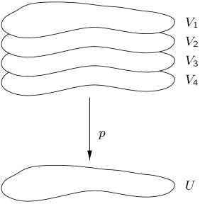
A continuous covering map $p:Y\rightarrow X$ is a continuous map from a connected topological space $Y$ to a connected topological space $X$ such that each $x$ in $X$ has a neighbourhood $U\subset X$ so that $p^{-1}(U)$ is a disjoint union of sets $\bigcup_{\beta\in\mathcal{B}}V_{\beta}$ , so that the restriction $p{}_{\mid V_{\beta}}{}$ is a homeomorphism for each $\beta\in\mathcal{B}$ . (See Figure 1.) We call $Y$ the covering space.

Refer to caption — Figure 1. Covering maps are ‘locally trivial’.

Notice that we consider only connected covering spaces.

Definition 6.2.

A smooth covering map $p:Y\rightarrow X$ is a continuous covering map so that the restrictions $p{}_{\mid V_{\beta}}{}$ are all diffeomorphisms.

Proposition 6.3.

If $p:Y\rightarrow X$ is a continuous covering map, and $X$ is a smooth manifold, then there is a unique differentiable structure for $Y$ so $p$ is a smooth covering map.

Proof.

We construct this smooth structure as follows. Let $\left(V_{\alpha}\right)_{\alpha\in\mathcal{A}}$ be an open covering of $Y$ by sets so that $p$ maps $V_{\alpha}$ homeomorphically onto its image, and $p(V_{\alpha})$ is a chart for $X$ , with coordinate map $\psi_{\alpha}:u(V_{\alpha})\rightarrow W_{\alpha}\subset\mathbb{R}^{n}$ for each $\alpha\in\mathcal{A}$ . Such an open covering certainly exists. Define $\varphi_{\alpha}:V_{\alpha}\rightarrow W_{\alpha}$ by $\varphi_{\alpha}(y)=\psi_{\alpha}(u(y))$ for each $\alpha\in\mathcal{A}$ . This map is a homeomorphism, because it is a composition of homeomorphisms. Further, the ‘transition maps’ $\varphi_{\alpha}{\circ}\varphi_{\alpha^{\prime}}^{-1}{}_{\mid W_{\alpha}\cap W_{\alpha^{\prime}}}{}$ are all diffeomorphisms, because $\varphi_{\alpha}{\circ}\varphi_{\alpha^{\prime}}^{-1}=\psi_{\alpha}{\circ}\psi_{\alpha^{\prime}}^{-1}$ . Thus the collection $\left(V_{\alpha},\varphi_{\alpha}\right)_{\alpha\in\mathcal{A}}$ defines an atlas for $Y$ , and it is clear that $p$ is a smooth map, and further a smooth covering map, with respect to this differentiable structure.

Uniqueness is trivial, since for $p$ to be a diffeomorphism, all of the charts described above must be in the atlas for $Y$ . The differentiable structure is uniquely determined by any atlas, establishing the result. ∎

Thus there is no essential difference between continuous and smooth covering maps.

Definition 6.4.

We say two continuous (respectively, smooth) covering maps $p:Y\rightarrow X$ and $p^{\prime}:Y^{\prime}\rightarrow X$ are equivalent if there is a homeomorphism (resp. diffeomorphism) $a:Y\rightarrow Y^{\prime}$ so $p^{\prime}{\circ}a=p$ .

6.2. Paths and loops

We next introduce the notions of paths and loops in a manifold. A path is a map $\left[0,1\right]\rightarrow M$ , and a loop is a map $\left[0,1\right]\rightarrow M$ taking $0$ and $1$ to the same point of $M$ . In this section, we will distinguish between continuous and smooth paths or loops, but we will also see that for the purposes of later sections this distinction is not important.

We say that two paths $\alpha,\beta$ such that $\alpha(0)=\beta(0)$ and $\alpha(1)=\beta(1)$ are continuously homotopic if there is a continuous map $H:\left[0,1\right]\times\left[0,1\right]\rightarrow M$ so that

	$\displaystyle H(0,t)$	$\displaystyle=\alpha(t)$
	$\displaystyle H(1,t)$	$\displaystyle=\beta(t)$
	$\displaystyle H(s,0)$	$\displaystyle=\alpha(0)=\beta(0)$
	$\displaystyle H(s,1)$	$\displaystyle=\alpha(1)=\beta(1).$

Two smooth paths are smoothly homotopic [40, §4] if there is such a smooth map $\left[0,1\right]\times\left[0,1\right]\rightarrow M$ . Again, we will see that this distinction is unimportant for our purposes, and so in later sections we always mean ‘smoothly homotopic’ by ‘homotopic’. Continuous homotopy gives an equivalence relation. It is clear that the relation is reflexive and symmetric. Continuous homotopies can be patched together, showing that continuous homotopy is a transitive relation. We thus denote the equivalence class of a path $\alpha$ under continuous homotopy by $[\alpha]$ .

Continuous paths can be concatenated. Given $\alpha,\beta:\left[0,1\right]\rightarrow M$ , such that $\alpha(0)=\beta(1)$ , the path $\alpha{\star}\beta:\left[0,1\right]\rightarrow M$ is defined by

(\alpha{\star}\beta)(t)=\left\{\begin{array}[]{ll}\beta(2t)&\textrm{if $t\in\left[0,\frac{1}{2}\right]$}\\ \alpha(2t-1)&\textrm{if $t\in\left[\frac{1}{2},1\right]$}\end{array}\right..

Smooth paths cannot necessarily be concatenated, as the resulting path may not be smooth at $t=\frac{1}{2}$ .

Concatenation is neither commutative nor associative. Up to homotopy, however, it is associative. That is, $[(\alpha{\star}\beta){\star}\gamma]=[\alpha{\star}(\beta{\star}\gamma)]$ for all paths $\alpha,\beta,\gamma$ such that these concatenations are defined. This relation is trivially proved by providing the appropriate homotopy. It is easy to see that $[\alpha{\star}\beta]$ depends only on the equivalence classes $[\alpha]$ and $[\beta]$ , so we can use the notation $[\alpha]{\star}[\beta]$ for $[\alpha{\star}\beta]$ .

The claim that the distinction between the continuous and smooth cases is unimportant follows from two facts.

Proposition 6.5.

Firstly, every continuous path in a smooth manifold is homotopic to a smooth path. Secondly, if two smooth paths are continuously homotopic, they are smoothly homotopic.

Proof.

See Theorem 7 and the following discussion in Chapter 2 of [48], and Theorem 8 of the same. Related results are given in [14, §16.26]. ∎

Given that henceforth we will work only in the smooth setting, it may seem redundant to have mentioned the continuous case at all. This infelicity is forced upon us by the fact that covering space theory is most natural in the continuous setting, and the theorems that we will rely on are proved there. On the other hand, much of the work described here, particularly the proofs in §7 of the Existence and Classification Theorems for spinor structures, and §8, relies intimately on smooth connections to provide accessible and geometric arguments. At the price of dealing here with both the continuous and the smooth case, we may later combine the power of both covering space theory and the theory of smooth connections. Additionally, of course, we want to work with smooth manifolds, so that we can do calculus.

With these results in hand, we can improve upon the theory of smooth paths and smooth homotopies. Firstly, we can define the equivalence relation of smooth homotopy. Again, it is clear that the relation is reflexive and symmetric. Now, if $\alpha,\beta,\gamma$ are three smooth paths so $\alpha$ is smoothly homotopic to $\beta$ , and $\beta$ is smoothly homotopic to $\gamma$ , then $\alpha$ must be continuously homotopic is $\gamma$ . Using the result that continuously homotopic smooth paths are smoothly homotopic, we see that smooth homotopy is also transitive. Again, we denote the smooth homotopy equivalence class of $\alpha$ by $[\alpha]$ . This overlap of notation is consistent. That is, the smooth paths in the smooth homotopy equivalence class of $\alpha$ are exactly the smooth paths in the continuous homotopy equivalence class of $\alpha$ .

Secondly, although smooth paths $\alpha,\beta$ with $\alpha(0)=\beta(1)$ cannot necessarily be concatenated, up to homotopy they can be.¹²¹²12This result, and the previous, that smooth homotopy is a transitive relation, can be proved more concretely, without the use of Proposition 6.5. See for example [40, §4]. Define $\lambda(t)=\frac{\mu(t-\frac{1}{3})}{\mu(t-\frac{1}{3})+\mu(\frac{2}{3}-t)},$ where $\mu(t)=0$ for $t\leq 0$ , and $\mu(t)=e^{-\frac{1}{t}}$ for $t>0$ . Then $\lambda:\left[0,1\right]\rightarrow\left[0,1\right]$ is smooth (but not analytic), and $\lambda([0,\frac{1}{3}])=0$ and $\lambda([\frac{2}{3}])=1$ . Using this, $\alpha{\circ}\lambda$ is smoothly homotopic to $\alpha$ , and for any smooth paths $\alpha,\beta$ such that $\alpha(0)=\beta(1)$ , $(\alpha{\circ}\lambda){\star}(\beta{\circ}\lambda)$ is a smooth path. A similar argument using $\lambda$ shows that smooth homotopy is transitive. This is because $\alpha$ and $\beta$ can be concatenated to form a continuous path $\alpha{\star}\beta$ , and this continuous path is homotopic to a smooth path. Thus we can define $[\alpha]{\star}[\beta]$ by $[\alpha{\star}\beta]$ . It is straightforward to see that $[\alpha]{\star}[\beta]$ depends only on the equivalence classes $[\alpha]$ and $[\beta]$ . Again, up to homotopy, concatenation is associative.

Concatenation always has a inverse, up to homotopy. If $\alpha$ is a path, we will write $\alpha^{-1}$ for the reverse path, defined by $\alpha^{-1}(t)=\alpha(1-t)$ . Then $[\alpha^{-1}{\star}\alpha]=[\alpha(0)]=[\alpha{\star}\alpha^{-1}]$ , where $[\alpha(0)]$ denotes the homotopy class of the constant path at $\alpha(0)$ .

6.3. Fundamental groups

We now introduce the fundamental group of a manifold. This construction requires a fixed base point in the manifold. Suppose $M$ is a smooth manifold, and $m_{0}\in M$ is a base point. Define $\Pi M$ to be the set of all smooth paths in $M$ starting at $m_{0}$ . Define $\Omega M$ to be the set of all smooth loops $\alpha$ in $M$ based at $m_{0}$ so $\alpha(0)=\alpha(1)=m_{0}$ , and $\Omega^{c}M$ to be the set of all continuous loops in $M$ . Define $\pi_{1}(M,m_{0})$ to be the set of smooth homotopy equivalence classes in $\Omega M$ , and give it a group structure by concatenation. Similarly define $\pi_{1}^{c}(M,m_{0})$ in the continuous case. In both cases the identity is given by the constant path at $m_{0}$ . We now reach the result which will allow us for the most part to dispense with the continuous case.

Proposition 6.6.

The map of $\pi_{1}(M,m_{0})$ into $\pi_{1}^{c}(M,m_{0})$ , taking the smooth homotopy equivalence class $[\alpha]$ to the continuous homotopy equivalence class $[\alpha]$ is an isomorphism.

Proof.

This follows immediately from Proposition 6.5. Firstly it is surjective, because any path in a smooth manifold is homotopic to a smooth path. Secondly, it is injective, since if two smooth paths are continously homotopic, they are smoothly homotopic. ∎

Henceforth we will not distinguish the continuous and smooth versions of the fundamental group. In particular, every element of the fundamental group has a smooth representative, and any two such representatives have a smooth homotopy between them. This will simplify our proofs, and will be vital in allowing certain constructions to work at all. With this knowledge in hand, we exclusively consider smooth paths, loops and homotopies, unless stated otherwise.

A map $\psi:X\rightarrow Y$ , taking $x_{0}$ to $y_{0}$ induces a homomorphism of the fundamental groups, from $\pi_{1}(X,x_{0})$ to $\pi_{1}(Y,y_{0})$ . This is given by $\psi_{*}:[\alpha]\mapsto[\psi{\circ}\alpha]$ . A moment’s consideration confirms this is a homomorphism and well defined on $\pi_{1}(X,x_{0})$ .

6.4. Classification of covering spaces

With the definitions of covering spaces and fundamental groups in place, we now state the main theorem for this section. It will be used in several places in the ensuing work.

Classification of Covering Spaces Theorem.

Let $P$ be a smooth connected manifold, with base point $\mathsf{p_{0}}$ .

For any covering space $Q$ of $P$ , with covering map $u:Q\rightarrow P$ and base point $\mathsf{q_{0}}\in u^{-1}(\mathsf{p_{0}})\subset Q$ , the induced map $u_{*}:\pi_{1}(Q,\mathsf{q_{0}})\rightarrow\pi_{1}(P,\mathsf{p_{0}})$ is injective.

For each subgroup $K\preceq\pi_{1}(P,\mathsf{p_{0}})$ , there exists a connected smooth covering space $Q$ of $P$ , with smooth covering map $u:Q\rightarrow P$ , and a base point $\mathsf{q_{0}}\in u^{-1}(\mathsf{p_{0}})\subset Q$ such that the image of $u_{*}:\pi_{1}(Q,\mathsf{q_{0}})\rightarrow\pi_{1}(P,\mathsf{p_{0}})$ is exactly $K$ .

Two coverings spaces $Q_{1}$ and $Q_{2}$ , with covering maps $u_{1}:Q_{1}\rightarrow P$ and $u_{2}:Q_{2}\rightarrow P$ and base points $\mathsf{q_{1}}\in u_{1}^{-1}(\mathsf{p_{0}})$ and $\mathsf{q_{2}}\in u_{2}^{-1}(\mathsf{p_{0}})$ respectively, are equivalent as in Definition 6.4 if and only if $u_{1*}(\pi_{1}(Q_{1},\mathsf{q_{1}}))$ and $u_{2*}(\pi_{1}(Q_{2},\mathsf{q_{2}}))$ are conjugate subgroups in $\pi_{1}(P,\mathsf{p})$ .

A preparatory remark. For the most part, smoothness is not particularly important in this theorem. The hypothesis that $P$ is a smooth manifold enables us to dispose easily of several of the necessary conditions for constructing covering spaces which occur in the continuous setting. The existence of smooth covering spaces follows very simply from the existence of continuous covering spaces.

Proof.

A complete proof of this theorem, as stated, cannot be found in any one place. Furthermore, for later work we will need some of the details of the constructions involved. For this reason, we present here an outline of the proof, citing appropriate references for each intermediate result, and in places extending standard results to fit the particular circumstances of this theorem.

The first part of the theorem, that the covering map induces an injective map of the fundamental groups, is very straightforward, using the lifting properties of covering maps. A proof is given in [19, §13], and [14, §16.28.4].

Next, we consider the implications of the smoothness of $P$ . Since $P$ is a manifold, it is locally path connected and locally simply connected, on account of each point of $P$ having a neighbourhood homeomorphic to an open ball in $\mathbb{R}^{n}$ . Further, connectedness implies that $P$ is path connected. This is because local path connectedness means that the path connected components of $P$ are open and closed, and so equal to connected components of $P$ . See also [42, §3-4].

The second part of the theorem, on existence of coverings, is proved in the continuous setting in [42, §8-14]. It depends upon $P$ being path connected, locally path connected, and locally (or semilocally) simply connected. As we have seen all these conditions are automatically true for smooth manifolds. To improve that result for this theorem, we need only show that this covering can be given a smooth structure so that the covering map becomes a smooth covering map, and this has already been achieved above, in Proposition 6.3. The statement about the fundamental groups remains true in the smooth setting, on account of Proposition 6.6.

Finally, the last part, giving conditions for equivalence of covering spaces, is proved in the continuous case in [42, §8-14]. To improve this for the current theorem, we need to show that if $u_{1}:Q_{1}\rightarrow P$ and $u_{2}:Q_{2}\rightarrow P$ are continuously equivalent covering maps, then they are smoothly equivalent covering maps, with respect to the differentiable structures defined above. This follows immediately from the definitions, and the fact that the continuous equivalence is given by a homeomorphism $a:Q_{1}\rightarrow Q_{2}$ such that $u_{2}{\circ}a=u_{1}$ , which is then also a diffeomorphism. ∎

A concluding remark. Later results will require some of the details of the construction of covering spaces. To that end, we describe this construction, and define the covering map. We will not explicitly describe the topology on the covering map. This is given in the references above, but we do not need the details beyond knowing that the covering map is in fact a covering map.

For a subgroup $K\preceq\pi_{1}(P,\mathsf{p_{0}})$ , the associated covering space $Q$ , as a set, is the collection of equivalence classes of paths in $P$ , starting at $\mathsf{p_{0}}$ , and ending anywhere in $P$ , with two such paths $\alpha$ and $\beta$ considered equivalent if $\alpha(1)=\beta(1)$ and the homotopy class ${[\alpha]^{-1}}{\star}{[\beta]}$ is in $K$ . We will write $\alpha{}^{\sharp}{}$ for the equivalence class of $\alpha$ . In particular, if $[\alpha]=[\beta]$ , then $\alpha{}^{\sharp}{}=\beta{}^{\sharp}{}$ . Moreover, if $[\gamma]\in K$ , then $[\alpha{\star}\gamma]^{-1}{\star}[\alpha]=[\gamma^{-1}]\in K$ , so $({\alpha}{\star}{\gamma}){}^{\sharp}{}=\alpha{}^{\sharp}{}$ . The covering map $u$ maps such a element of $Q$ to its endpoint. Thus $u([\alpha])=\alpha(1)$ . This is clearly well defined.

Corollary.

Every smooth connected manifold has a universal covering manifold, that is, a simply connected smooth covering space. Further, this is essentially unique.

Proof.

Take the trivial subgroup $\langle e\rangle$ in $\pi_{1}(P,\mathsf{p_{0}})$ , and form the associated covering space $Q$ . Since the covering map $u$ induces an injective map $\pi_{1}(Q,\mathsf{q_{0}})\rightarrow\langle e\rangle$ , $\pi_{1}(Q,\mathsf{q_{0}})$ is itself trivial, and so $Q$ is simply connected. If $u^{\prime}:Q^{\prime}\rightarrow P$ is any other covering map with $Q^{\prime}$ simply connected with base point $\mathsf{q^{\prime}_{0}}$ , then $u^{\prime}_{*}:\pi_{1}(Q^{\prime},\mathsf{q^{\prime}_{0}})\rightarrow\pi_{1}(P,\mathsf{p_{0}})$ has a trivial image, and so the covering map $u^{\prime}:Q^{\prime}\rightarrow P$ is equivalent to the one we have constructed, $u:Q\rightarrow P$ . ∎

6.5. Covering spaces of Lie groups

Given a connected Lie group $G$ we can form its universal covering manifold $\widetilde{G}$ , with covering map $\rho:\widetilde{G}\rightarrow G$ . We always consider the identity $e$ to be the base point of a group. Fix some $\widetilde{e}\in\rho^{-1}(e)$ , the inverse image of the identity in $G$ .

Proposition 6.7.

This manifold $\widetilde{G}$ has a unique group structure with identity $\widetilde{e}$ so that $\rho$ becomes a homomorphism.

Proof.

This is proved in [14, §16.30]. ¹³¹³13An alternative, less abstract sketch proof is as follows. The fact that $\rho$ is locally a diffeomorphism near $\widetilde{e}$ ensures that there is a unique group structure on a neighbourhood of $\widetilde{e}$ . By path connectedness, and the Lebesgue number lemma [42, §3-7], every element of the group is a finite product of elements of this neighbourhood. This extends the local group structure to a group structure for the entire manifold. We then have to check that it is well defined. For the sake of brevity, we will not do the details here. ∎

We will henceforth always mean the group when we write $\widetilde{G}$ , and call it the universal covering group.

According to the construction given in the Classification of Covering Spaces Theorem, the set underlying $\widetilde{G}$ is the set of homotopy classes of paths in $G$ starting at $e$ and ending somewhere in the group $G$ . The covering map $\rho:\widetilde{G}\rightarrow G$ then takes such a class of paths to the common endpoint.

Example.

Familiar Lie groups with well known covering groups are $S^{1}$ , covered by $\mathbb{R}$ , where the covering map is $x\mapsto e^{2\pi ix}$ , and $SO(3)$ , covered by $SU(2)$ . In Part III we will be particularly concerned with the double covering of $SO_{0}(1,3)$ by $SL(2,\mathbb{C})$ . This is the physically relevant group in relativity theory.

7. Spinor structures

It is at this point, when we come to define a spinor structure, that the effort required to reformulate geometrically the ideas of metrics and compatible covariant derivatives in terms of orthonormal bundles and connections thereon comes to fruition. The spinor structure will be explicitly constructed from the orthonormal bundle. The alternative approach to spinors, which is more common, is interested only in the algebraic side, and mostly proceeds from the axioms for a spinor algebra [47]. (Compare §12.) The comparison of constructive and axiomatic viewpoints in [47, pp. 211–212] is especially worthwhile.

For the following definition, take $G$ to be a connected but not simply connected Lie group, and $\widetilde{G}$ to be its universal covering group. The covering map will be denoted $\rho:\widetilde{G}\rightarrow G$ .

Definition.

Given a $G$ principal fibre bundle $G\rightsquigarrow P\xrightarrow{\smash[t]{\pi_{P}}}M$ , a spinor structure is a $\widetilde{G}$ principal fibre bundle $\widetilde{G}\rightsquigarrow Q\xrightarrow{\smash[t]{\pi_{Q}}}M$ , along with a principal fibre bundle morphism relative to $\rho$ , that is, a map $u:Q\rightarrow P$ , so that $u(\mathsf{q}\widetilde{g})=u(\mathsf{q})\rho(\widetilde{g})$ , for all $\mathsf{q}\in Q$ and $\widetilde{g}\in\widetilde{G}$ . We call $u$ the spinor map.

This definition implies in particular that the projection maps are related according to

\pi_{Q}=\pi_{P}{\circ}u.

Accordingly, given a pseudo-Riemannian manifold, and suitable orientations, we have seen that there is a corresponding $SO_{0}(p,q)$ principal fibre bundle, which we have called the orthonormal bundle. A spinor structure for such a pseudo-Riemannian manifold is then just a spinor structure for this bundle. Having recast pseudo-Riemannian geometry in terms of principal fibre bundles, the theory of spinor structures for pseudo-Riemannian manifolds can be subsumed into the general discussion that we give here. We will see also that the correspondence between covariant derivatives and connections on an orthonormal bundle fits into this theory. In §9 we show how to generate connections on a spinor structure from connections on the original bundle.

In the special case of a $(1+3)$ dimensional Lorentz structure, where $G=SO_{0}(1,3)$ and $\Lambda M$ is an orthonormal frame bundle, a spinor structure is an $SL(2,\mathbb{C})$ principal fibre bundle $\Sigma M$ , along with a map $u:\Lambda M\rightarrow\Sigma M$ , so $u(\mathsf{q}g)=u(\mathsf{q})\rho(g)$ for all $g\in SL(2,\mathbb{C})$ , where $\rho$ is the two fold covering map described in detail in §11.

We will next state the main results on the existence and uniqueness of spinor structures. We will later be particularly interested in the case of Lorentz bundles and $SL(2,\mathbb{C})$ bundles. However the discussion will apply to the more general situation. Investigating the general case allows us later to discuss the degree to which the choice of metric on a manifold affects the existence and classification of the spinor structures, in §8.

To begin, we need the following fundamental lemma relating spinor structures and covering maps.

Lemma 7.1.

If $Q$ is a spinor structure for the bundle $P$ , the principal fibre bundle morphism $u:Q\rightarrow P$ is a covering map.

Proof.

Consider a local cross section of $Q$ , defined on an open subset $U\subset M$ , $\sigma:U\rightarrow Q$ . The composition $u{\circ}\sigma$ then defines a local cross section of $P$ . We can use these cross sections to define local trivialisations of both bundles, by Lemma 1.2.

$\displaystyle\psi:$	$\displaystyle U\times\widetilde{G}$	$\displaystyle\rightarrow\pi_{Q}^{-1}(U)$
	$\displaystyle(m,\widetilde{g})$	$\displaystyle\mapsto\sigma(m)\widetilde{g}$
$\displaystyle\varphi:$	$\displaystyle U\times G$	$\displaystyle\rightarrow\pi_{P}^{-1}(U)$
	$\displaystyle(m,g)$	$\displaystyle\mapsto u(\sigma(m))g$

Both of these maps are diffeomorphisms, and in fact principal morphisms. We can compose these maps with $u$ , to obtain

\varphi^{-1}{\circ}u{\circ}\psi:U\times\widetilde{G}\rightarrow U\times G.

However this map acts very simply, as follows,

$\displaystyle\left(\varphi^{-1}{\circ}u{\circ}\psi\right)(m,\widetilde{g})$	$\displaystyle=$	$\displaystyle(\varphi^{-1}{\circ}u)(\sigma(m)\widetilde{g})$
	$\displaystyle=$	$\displaystyle\varphi^{-1}(u(\sigma(m))\rho(\widetilde{g}))$
	$\displaystyle=$	$\displaystyle(m,\rho(\widetilde{g})).$

Thus $\varphi^{-1}{\circ}u{\circ}\psi=\operatorname{id}_{M}\times\rho$ , and as $\psi$ and $\varphi$ are diffeomorphisms, we can write the covering map as $u{}_{\mid\pi_{Q}^{-1}(U)}{}=\varphi{\circ}(\operatorname{id}_{M}\times\rho){\circ}\psi^{-1}$ . This expresses $u$ locally as a trivial map in the sense of covering spaces, and so $u$ is a covering map. ∎

This enables us to apply the powerful Classification of Covering Spaces Theorem to the task at hand. It also indicates the dual appearance of covering space theory in the description of a spinor structure. To look for a principal fibre bundle whose structure group has been ‘unwrapped’ to the simply connected covering group, we must ‘unwrap’ the bundle itself. This is not always possibly, and we will see that the desired covering bundle is not itself simply connected, and so need not be unique when one does exist.

An immediate and simple result of Lemma 7.1 and the Classification of Covering Spaces Theorem is the following.

Proposition 7.2.

If the fundamental group of $P$ is trivial then there is no spinor structure.

Proof.

Since $P$ is simply connected, every covering space is equivalent to $P$ itself, and so $P$ has no connected covering spaces larger than itself, and thus no spinor structure is possible. ∎

Next, we need to say exactly what we mean by ‘classification’ of spinor structures, by defining what it means to say that two are equivalent.

Definition 7.3.

Two spinor structures

\widetilde{G}\rightsquigarrow Q\xrightarrow{\smash[t]{\pi_{Q}}}M\quad\text{and}\quad\widetilde{G}\rightsquigarrow Q^{\prime}\xrightarrow{\smash[t]{\pi_{Q^{\prime}}}}M

with spinor maps $u:Q\rightarrow P$ and $u^{\prime}:Q^{\prime}\rightarrow P$ respectively are said to be equivalent is there is a principal fibre bundle morphism $a:Q\rightarrow Q^{\prime}$ such that $u=u^{\prime}{\circ}a$ .

The main results of this section are summarised by the following theorems.

We begin by defining the map $i:G\rightarrow P$ by $i(g)=\mathsf{p_{0}}g$ . This induces a homomorphism $i_{*}:\pi_{1}(G)\rightarrow\pi_{1}(P)$ .

Existence Theorem.

A principal fibre bundle $G\rightsquigarrow P\xrightarrow{\smash[t]{\pi_{P}}}M$ has a spinor structure if and only if the fundamental group of the bundle $\pi_{1}(P)$ can be written as a direct product of subgroups $K$ and $I$ ,

\pi_{1}(P)=K\times I,

such that $K$ and $I$ have trivial intersection, and $\pi_{P*}$ maps $K$ isomorphically to $\pi_{1}(M)$ and $i_{*}$ maps $\pi_{1}(G)$ isomorphically to $I$ .¹⁴¹⁴14We could state this condition more concisely, but more abstractly, as ‘there is a short exact sequence and this sequence is split’. We will not be thinking in these terms however.

Note that if $P$ is trivial, so $P=M\times G$ , then there is an obvious spinor structure, given by $Q=M\times\widetilde{G}$ , and $u:Q\rightarrow P$ according to $u(m,\widetilde{g})=(m,\rho(\widetilde{g}))$ . In this case the theory of fundamental groups shows that $\pi_{1}(P)=\pi_{1}(M)\times\pi_{1}(G)$ . We can think of the existence theorem as the statement that even if $P$ is not trival, to have a spinor structure ‘its fundamental group must look as if $P$ is trivial’.

Classification Theorem.

In the case that the conditions of the Existence Theorem obtain, the inequivalent spinor structures are in one to one correspondence with the homomorphisms from $\pi_{1}(M)\rightarrow\pi_{1}(G)$ .

This is a ‘relative’ classification. Given a particular spinor structure, each of the other spinor structures corresponds to a particular nontrivial homomorphism $\pi_{1}(M)\rightarrow\pi_{1}(G)$ .

To reach these results, we will first establish the necessary conditions for the existence of a spinor structure. This is achieved in §7.1. That these conditions are sufficient will follow, in §7.2, and subsequently we will describe the classification of spinor structures in §7.3.

7.1. Necessary conditions

Suppose now that there exists a spinor structure $Q$ for $P$ , with spinor map $u:Q\rightarrow P$ . The four main results that follow from this are Propositions 7.4, 7.5, 7.7 and 7.8. Together, these establishe the necessity of the conditions in the Existence Theorem.

Proposition 7.4.

The map

\pi_{Q*}:\pi_{1}(Q)\rightarrow\pi_{1}(M)

is an isomorphism.

Proof.

For the purposes of this proof, we will fix a connection on $Q$ . Such a connection always exists by the results in §5.1.

Proving that $\pi_{Q*}$ is surjective is relatively easy, so we first do that.

Suppose $\alpha$ is any smooth loop in $M$ based at $m_{0}$ . Define $\widetilde{\alpha}_{\mathsf{q_{0}}}$ to the parallel transport of $\mathsf{q_{0}}\in\pi_{Q}^{-1}(m_{0})$ along $\alpha$ . This curve will generally not be a loop. However, $\pi_{Q}(\widetilde{\alpha}_{\mathsf{q_{0}}}(1))=m_{0}$ , and since the fibres of $Q$ are path connected, we can find a path $\delta:\left[0,1\right]\rightarrow\widetilde{G}$ so $\delta(0)=\widetilde{e}$ and $\delta(1)=\tau(\widetilde{\alpha}_{\mathsf{q_{0}}}(1),\mathsf{q_{0}})$ . Now consider the path $\widetilde{\alpha}_{\mathsf{q_{0}}}\delta$ , which is in fact a loop since $(\widetilde{\alpha}_{\mathsf{q_{0}}}\delta)(0)=\mathsf{q_{0}}$ and $(\widetilde{\alpha}_{\mathsf{q_{0}}}\delta)(1)=\widetilde{\alpha}_{\mathsf{q_{0}}}(1)\tau(\widetilde{\alpha}_{\mathsf{q_{0}}}(1),\mathsf{q_{0}})=\mathsf{q_{0}}$ . Further $\pi_{Q}(\widetilde{\alpha}_{\mathsf{q_{0}}}\delta)=\pi_{Q}(\widetilde{\alpha}_{\mathsf{q_{0}}})=\alpha$ , and so $\pi_{Q*}[\widetilde{\alpha}_{\mathsf{q_{0}}}\delta]=[\alpha]$ . Thus $\pi_{Q*}$ is surjective.

We now turn to the more technical problem of demonstrating that $\pi_{Q*}$ is injective. The underlying result, however, has already been established, the idea here being to use a connection to ‘lift’ a homotopy in $M$ to a map into $Q$ , and then using the simply connectedness of fibres to modify this into the appropriate homotopy. Suppose $[\alpha]$ and $[\beta]$ are elements of $\pi_{1}(Q)$ , and $\pi_{Q*}([\alpha])=\pi_{Q*}([\beta])$ . Then there are smooth loops $\gamma_{0}$ and $\gamma_{1}$ in $M$ , so $[\gamma_{0}]=\pi_{Q*}([\alpha])$ and $[\gamma_{1}]=\pi_{Q*}([\beta])$ , and, further, there are smooth loops $\alpha^{\prime}$ and $\beta^{\prime}$ in $Q$ so $[\alpha]=[\alpha^{\prime}]$ , $[\beta]=[\beta^{\prime}]$ and $\pi_{Q}(\alpha^{\prime})=\gamma_{0}$ , and $\pi_{Q}(\beta^{\prime})=\gamma_{1}$ . Thus there is a smooth homotopy from $\gamma_{0}$ to $\gamma_{1}$ . Call this homotopy $\gamma$ , so $\gamma(0,t)=\gamma_{0}(t)$ , and $\gamma(1,t)=\gamma_{1}(t)$ . We will write $\gamma_{s}$ for the function $t\mapsto\gamma(s,t)$ . According to the second part of Proposition 5.4, we can parallel transport $\mathsf{q_{0}}$ along $\gamma_{s}$ , to obtain a smooth curve $\widetilde{\gamma_{s}}_{\mathsf{q_{0}}}$ , so that $\pi_{Q}(\widetilde{\gamma_{s}}_{\mathsf{q_{0}}}(t))=\gamma(s,t)$ , and the map $H:(s,t)\mapsto\widetilde{\gamma_{s}}_{\mathsf{q_{0}}}(t)$ is continuous. We will next modify $H$ to form a homotopy between $\alpha^{\prime}$ and $\beta^{\prime}$ .

The particular properties of $H$ that we require are

	$\displaystyle H(s,0)$	$\displaystyle=\mathsf{q_{0}},$
	$\displaystyle\pi_{Q}(H(0,t))$	$\displaystyle=\gamma_{0}(t)=\pi_{Q}(\alpha^{\prime}(t)),$
	$\displaystyle\pi_{Q}(H(1,t))$	$\displaystyle=\gamma_{1}(t)=\pi_{Q}(\beta^{\prime}(t)),\textrm{ and}$
	$\displaystyle\pi_{Q}(H(s,1))$	$\displaystyle=m_{0}=\pi_{Q}(\mathsf{q_{0}}).$

Define $\partial$ to be the boundary of $\left[0,1\right]\times\left[0,1\right]$ , that is

\partial=\left(\{0,1\}\times\left[0,1\right]\right)\cup\left(\left[0,1\right]\times\{0,1\}\right).

Define $\zeta:\partial\rightarrow Q$ according to $\zeta(s,0)=\zeta(s,1)=\mathsf{q_{0}}$ for all $s\in\left[0,1\right]$ , and $\zeta(0,t)=\alpha^{\prime}(t)$ , $\zeta(1,t)=\beta^{\prime}(t)$ . According to this definition, and the above properties of $H$ , $\pi_{Q}{\circ}\zeta=\pi_{Q}\circ H{}_{\mid\partial}{}$ on $\partial$ , and so $\zeta=(H{}_{\mid\partial}{})\widetilde{g}$ , for some function $\widetilde{g}:\partial\rightarrow\widetilde{G}$ . Since $\widetilde{G}$ is simply connected, we can extend $\widetilde{g}$ to a continuous function $\widetilde{g}:\left[0,1\right]\times\left[0,1\right]\rightarrow\widetilde{G}$ . Now define $K:\left[0,1\right]\times\left[0,1\right]\rightarrow Q$ by $K=H\widetilde{g}$ . Thus on $\partial$ , $K$ and $\zeta$ agree, and so $K$ is a continuous homotopy between $\alpha^{\prime}$ and $\beta^{\prime}$ . Finally, this implies that there is a continuous homotopy between $\alpha$ and $\beta$ , and so by Proposition 6.5, there is a smooth homotopy between $\alpha$ and $\beta$ . This establishes the injectivity of $\pi_{Q*}$ , and so proves that it is an isomorphism. ∎

Proposition 7.5.

Let $K=u_{*}(\pi_{1}(Q))\preceq\pi_{1}(P)$ . Then the restriction of $\pi_{P*}$ to $K$ , mapping $K$ to $\pi_{1}(M)$ , is an isomorphism.

Proof.

Firstly, the map $u_{*}:\pi_{1}(Q)\rightarrow\pi_{1}(P)$ is injective, according to the Covering Space Classification Theorem. We now consider the following commuting diagram,

and the restriction of $\pi_{P*}$ to $K$ , $(\pi_{P*}){}_{\mid K}{}$ . Since $u_{*}$ is injective and $\pi_{Q*}$ is an isomorphism, by Proposition 7.4, $(\pi_{P*}){}_{\mid K}{}$ is injective. Further, $(\pi_{P*}){}_{\mid K}{}u_{*}=\pi_{Q*}$ , so $(\pi_{P*}){}_{\mid K}{}$ must be surjective, and thus $(\pi_{P*}){}_{\mid K}{}$ is an isomorphism. ∎

An important property of the map $i:G\rightarrow P$ is that $i_{*}$ maps $\pi_{1}(G)$ into the centre of $\pi_{1}(P)$ . This is made clear by the following Lemma.

Lemma 7.6.

Suppose $g\in\Pi G$ , and $\alpha\in\Pi P$ . Then

\left[\alpha g\right]=\left[{(\alpha g(1))}{\star}{i(g)}\right].

If $g\in\Omega G$ , and $\alpha\in\Omega P$ , then

\left[{i(g)}{\star}{\alpha}\right]=\left[\alpha g\right]=\left[{\alpha}{\star}{i(g)}\right].

Thus $i_{*}:\pi_{1}(G)\rightarrow Z(\pi_{1}(P))$ .

Proof.

See §C.3. ∎

It should also be pointed out that $\pi_{1}(G)$ is always itself commutative when $G$ is a Lie group, as discussed in Lemma A.1.

Proposition 7.7.

The map $i_{*}:\pi_{1}(G)\rightarrow\pi_{1}(P)$ is injective, and so if we define $I=i_{*}(\pi_{1}(G))\preceq\pi_{1}(P)$ , then $i_{*}:\pi_{1}(G)\rightarrow I$ is an isomorphism.

Proof.

Suppose $[g]\in\pi_{1}(G)$ , and $i_{*}[g]=[\alpha]$ . Suppose $\alpha$ is homotopically trivial. Then, according to the Path Lifting Lemma [42, §8-4] we can lift $\alpha$ via the covering map $u$ to a path $\widetilde{\alpha}$ in $Q$ , and according to the Homotopy Lifting Lemma [42, §8-4], it is a loop homotopic to the constant loop. This loop lies within a single fibre, and, since the fibres are homeomorphic to $\widetilde{G}$ , they are simply connected, and so $\widetilde{\alpha}$ is homotopic to the constant loop by a homotopy that stays within the fibre $\pi_{Q}^{-1}(m_{0})$ . Applying $u$ to this homotopy gives a homotopy of $\alpha$ to the constant loop by a homotopy that stays within the fibre $\pi_{P}^{-1}(m_{0})$ , and thus $g$ is homotopic to the constant loop in $G$ . Thus $[g]=[e]$ , and so $i_{*}$ is injective. ∎

Proposition 7.8.

The groups $K$ and $I$ have trivial intersection in $\pi_{1}(P)$ , and the internal direct product $K\times I$ is exactly $\pi_{1}(P)$ .

Proof.

The proof is in two steps.

Say $[\alpha]\in K$ , $[g]\in\pi_{1}(G)$ , and $[\alpha]=i_{*}[g]$ . Then, applying $\pi_{P*}$ to both sides,

\pi_{P*}[\alpha]=\pi_{P*}i_{*}[g]=[e],

since $i_{*}[g]$ has a representative lying within a single fibre. Now, since $\pi_{P*}$ restricted to $K$ is an isomorphism, $[\alpha]=[e]$ also, and since $i_{*}$ is injective by Proposition 7.7, $[g]=[e]$ as well. Thus the two groups have a trivial intersection.

Next, take any $[\alpha]\in\pi_{1}(P)$ . We define $[\hat{\alpha}]\in K\preceq\pi_{1}(P)$ as follows. Firstly let $\beta=\pi_{P}{\circ}\alpha:\left[0,1\right]\rightarrow M$ . Then, as in the discussion of Proposition 7.4, let $\beta^{\prime}=\widetilde{\beta}_{\mathsf{q_{0}}}:\left[0,1\right]\rightarrow Q$ be the parallel transport of $\mathsf{q_{0}}$ along $\beta$ . Further, chose a path $\delta:\left[0,1\right]\to\widetilde{G}$ so $\delta(0)=\widetilde{e}$ and $\beta^{\prime\prime}=\beta^{\prime}\delta$ is a loop in $Q$ . Now $\pi_{Q}{\circ}\beta^{\prime\prime}=\pi_{Q}{\circ}\beta^{\prime}=\pi_{P}{\circ}\alpha$ . Define $\hat{\alpha}$ = $u{\circ}\beta^{\prime\prime}$ . We see from this, and Proposition 7.4, that $[\hat{\alpha}]=u_{*}\pi_{Q*}{}^{-1}\pi_{P*}[\alpha]$ , and moreover that $\pi_{P}{\circ}\hat{\alpha}=\pi_{P}{\circ}\alpha$ .

Thus $\alpha=\hat{\alpha}g$ for some loop $g:\left[0,1\right]\rightarrow G$ . Then

	$\displaystyle[\alpha]$	$\displaystyle=[\hat{\alpha}g]$
		$\displaystyle={[\hat{\alpha}]}{\star}{i_{*}[g]},$

applying Lemma 7.6. Thus the internal direct product $K\times I$ generates all of $\pi_{1}(P)$ . ∎

7.2. Sufficient conditions

Now we suppose the conditions stated in the Existence Theorem. That is, suppose that $P$ is the total space of a $G$ principal fibre bundle over $M$ , and that there is a subgroup $K$ of $\pi_{1}(P)$ isomorphic to $\pi_{1}(M)$ via $\pi_{P*}$ such that $\pi_{1}(P)=K\times i_{*}(\pi_{1}(G))$ . We will show that these conditions are sufficient for the existence of a spinor structure $Q$ .

Let $Q$ be the covering space of $P$ associated with the subgroup $K$ , according to the Covering Space Classification Theorem, and $u$ be the corresponding covering map. There is a base point $\mathsf{q_{0}}\in u^{-1}(\mathsf{p_{0}})\subset Q$ so that $u_{*}$ maps $\pi_{1}(Q,\mathsf{q_{0}})\rightarrow K\preceq\pi_{1}(P,\mathsf{p_{0}})$ and is injective. Define the projection map $\pi_{Q}:Q\rightarrow M$ by $\pi_{Q}=\pi_{P}{\circ}u$ .

We now define a $\widetilde{G}$ action on $Q$ . We will then show that with respect to this action $Q$ becomes a $\widetilde{G}$ principal fibre bundle, and $u$ a principal morphism relative to $\rho:\widetilde{G}\rightarrow G$ .

Fix $\mathsf{q}\in Q$ and $\widetilde{g}\in\widetilde{G}$ . According to the construction of the covering space, outlined in the remark following the proof of the Covering Space Classification theorem, $\mathsf{q}$ is an equivalence class of paths in $P$ , written $\alpha{}^{\sharp}{}$ , for some $\alpha:\left[0,1\right]\rightarrow P$ , with $\alpha(0)=\mathsf{p_{0}}$ . Two such paths are equivalent, $\alpha{}^{\sharp}{}=\beta{}^{\sharp}{}$ , if $\alpha(1)=\beta(1)$ and $[\alpha^{-1}{\star}\beta]\in K$ . Since $\widetilde{G}$ is the universal covering group of $G$ , $\widetilde{g}$ can be thought of as a homotopy class of paths in $G$ starting at the identity, as in §6.5. Choose a path from this homotopy class, and denote it $g:\left[0,1\right]\rightarrow G$ , so $g(0)=e$ . The $G$ action on $P$ allows us to define a path $\alpha g:\left[0,1\right]\rightarrow P$ by $(\alpha g)(t)=\alpha(t)g(t)$ . Define the action of $\widetilde{g}$ on $\mathsf{q}$ by $\mathsf{q}\widetilde{g}=(\alpha g){}^{\sharp}{}$ . According to the first part of Lemma 7.6, $\left[\alpha g\right]=\left[{(\alpha g(1))}{\star}{i(g)}\right]$ , and so we can alternatively write

\mathsf{q}\widetilde{g}=({(\alpha g(1))}{\star}{i(g)}){}^{\sharp}{}.

(7.1)

These paths are illustrated in Figure 2.

This is clearly independent of the particular path $g$ we have chosen, because homotopic paths in $P$ are equivalent as points in $Q$ . To check that this definition is also independent of the representative of $\alpha{}^{\sharp}{}$ , we suppose $\alpha{}^{\sharp}{}=\beta{}^{\sharp}{}$ , so $[\beta^{-1}{\star}\alpha]\in K$ . Then $[(\beta g)^{-1}{\star}(\alpha g)]=[\beta^{-1}{\star}i(g^{-1}){\star}i(g){\star}\alpha]\in K$ , using Lemma 7.6, and so $(\alpha g){}^{\sharp}{}=(\beta g){}^{\sharp}{}$ .

We have now defined the projection map $\pi_{Q}$ and the $\widetilde{G}$ action on $Q$ . Our claim is that these provide a spinor structure for $P$ . Thus the remainder of the proof of the Existence Theorem is contained in the following two results. Proposition 7.9 checks the consistency of $\pi_{Q}$ and the $\widetilde{G}$ action, in the sense that together they satisfy the axioms for a principal fibre bundle, in Definition 1.1. Lemma 7.10 then proves that $u$ , the covering map from $Q$ to $P$ , is in fact a principal morphism relative to $\rho$ , respecting the principal fibre bundle structures of $Q$ and $P$ .

Proposition 7.9.

The above construction of $\widetilde{G}\rightsquigarrow Q\xrightarrow{\smash[t]{\pi_{Q}}}M$ is in fact a principal fibre bundle. Specifically, the $\widetilde{G}$ action on $Q$ must be

free:: in the sense that if $\mathsf{q}\widetilde{g}=\mathsf{q}$ for any $\mathsf{q}\in Q$ , then $\widetilde{g}=e$ , and,
transitive on fibres:: so if $\mathsf{q},\mathsf{q^{\prime}}\in Q$ are such that $\pi_{Q}(\mathsf{q})=\pi_{Q}(\mathsf{q^{\prime}})$ , then there is some $\widetilde{g}\in\widetilde{G}$ so that $\mathsf{q^{\prime}}=\mathsf{q}\widetilde{g}$ .

Further, there must be local trivialisations of $Q$ compatible with the $\widetilde{G}$ action.

Proof.

The proof is in three parts. All are straightforward, but somewhat involved, especially the second.

The action is free. Suppose $\widetilde{g}\in\widetilde{G}$ is such that $\mathsf{q}\widetilde{g}=\mathsf{q}$ for some $\mathsf{q}=\alpha{}^{\sharp}{}\in Q$ . Take a path in $G$ representing $\widetilde{g}$ , say $g:\left[0,1\right]\rightarrow G$ , so $g(1)=\rho(\widetilde{g})$ . As in Equation (7.1), $\mathsf{q}\widetilde{g}=((\alpha g(1)){\star}i(g)){}^{\sharp}{}$ . Then $\mathsf{q}\widetilde{g}=\mathsf{q}$ implies

	$\displaystyle{[\alpha]^{-1}}{\star}{[{(\alpha g(1))}{\star}{i(g)}]}$	$\displaystyle=[i(g)]$
		$\displaystyle\in K,$

and so $[i(g)]=[e]$ , by the hypothesis that $\pi_{1}(P)=K\times i(\pi_{1}(G))$ . Thus $g$ is homotopically trivial, and so $\widetilde{g}=e$ .

The action is transitive. Suppose we have two elements $\mathsf{q},\mathsf{q^{\prime}}$ of $Q$ within the same fibre, such that $\mathsf{q}=\alpha{}^{\sharp}{}$ and $\mathsf{q^{\prime}}=\beta{}^{\sharp}{}$ for two paths $\alpha,\beta:\left[0,1\right]\rightarrow P$ . Since $\mathsf{q}$ and $\mathsf{q^{\prime}}$ are in the same fibre, $\alpha(1),\beta(1)\in{\pi_{P}}^{-1}(m)$ for some $m\in M$ . Consider ${[\beta]^{-1}}{\star}{[{\alpha g}{\star}{\gamma}]}$ for some $[\gamma]\in K\subset\pi_{1}(P)$ , and $g:\left[0,1\right]\rightarrow G$ so $g(0)=e$ and $\alpha(1)g(1)=\beta(1)$ . Such a $g$ exists since $G$ is path connected, and $G$ acts transitively on the fibres of $P$ . Further, $g$ represents some $\widetilde{g}\in\widetilde{G}$ . We calculate

	$\displaystyle[\beta]^{-1}{\star}[\alpha g{\star}\gamma]$	$\displaystyle=[\beta^{-1}{\star}\alpha g(1){\star}i(g){\star}\gamma]$
		$\displaystyle=[\beta^{-1}{\star}\alpha g(1){\star}i(h^{-1}){\star}i(h{\star}g){\star}\gamma]$
		$\displaystyle=[\beta^{-1}{\star}\alpha g(1){\star}i(h^{-1}){\star}\gamma{\star}i(h{\star}g)].$

Here $h:\left[0,1\right]\rightarrow G$ is any path in $G$ so $h(0)=g(1)$ and $h(1)=e$ , and $h^{-1}$ denotes the reversed path $h^{-1}(t)=h(1-t)$ , not the inverse path, and we have used Lemma 7.6 in the last line. Note that by varying $g$ , subject still to the conditions $g(0)=e$ and $\alpha(1)g(1)=\beta(1)$ , we can make $h{\star}g$ homotopic to any arbitrary loop $j$ in $G$ . This is achieved by setting $g=h^{-1}{\star}j$ , so $[h{\star}g]=[j]$ . Thus the first two paths, $\gamma$ and $i(h{\star}g)$ can be chosen to generate any element of $\pi_{1}(P)$ , since $\pi_{1}(P)=K\times i(\pi_{1}(G))$ . In particular, we can chose $g$ and $\gamma$ so that

[\gamma{\star}i(h{\star}g)]=[\beta^{-1}{\star}\alpha g(1){\star}i(h^{-1})]^{-1},

[\beta]^{-1}{\star}[\alpha g{\star}\gamma]=[e]\in K.

With this choice,

\mathsf{q^{\prime}}=\beta{}^{\sharp}{}=\alpha g{\star}\gamma{}^{\sharp}{}=\alpha g{}^{\sharp}{}=\mathsf{q}\widetilde{g}.

This proves that the $\widetilde{G}$ action is transitive on the fibres, as required.

There are local trivialisations compatible with the $\widetilde{G}$ action. Since $P$ is a principal fibre bundle, for any point $m_{0}\in M$ there is an open set $V$ with $m_{0}\in V\subset M$ and a local section $\sigma:V\rightarrow P$ , in accordance with Lemma 1.2. Find a simply connected open set $U\subset V$ , and restrict $\sigma$ to $U$ . By the monodromy principle [14, §16.28.8] there is a lifting of $\sigma$ to a map $\widetilde{\sigma}:U\rightarrow Q$ via the covering map $u$ . This is then a local section of $Q$ , and applying Lemma 1.2 a second time we find a local trivialisation. ∎

The final step in establishing that our construction generates a spinor structure is now easy.

Lemma 7.10.

The map $u:Q\rightarrow P$ is a principal morphism relative to $\rho$ .

Proof.

In the notation above $\rho$ acts on $\widetilde{G}$ by taking $\widetilde{g}$ to $g(1)$ . Thus

	$\displaystyle u(\mathsf{q}\widetilde{g})$	$\displaystyle=u((\alpha g){}^{\sharp}{})$
		$\displaystyle=\alpha(1)g(1)$
		$\displaystyle=u(\mathsf{q})\rho(\widetilde{g}).$

Following from these results, we obtain the following statement about the spinor structure equivalence, which will be vital in proving the classification in §7.3.

Proposition 7.11.

Two spinor structures $u:Q\rightarrow P$ and $u^{\prime}:Q^{\prime}\rightarrow P$ are equivalent (in the sense of Definition 7.3) if and only if they are equivalent as covering maps (Definition 6.4).

Proof.

If $u:Q\rightarrow P$ and $u^{\prime}:Q^{\prime}\rightarrow P$ are equivalent as spinor structures then there is a principal bundle morphism $a:Q\rightarrow Q^{\prime}$ so $u=u^{\prime}{\circ}a$ . This $a$ is then a fortiori a diffeomorphism, and so $u$ and $u^{\prime}$ are immediately seen to be equivalent as covering maps.

Conversely, suppose $u:Q\rightarrow P$ and $u^{\prime}:Q^{\prime}\rightarrow P$ are equivalent as covering spaces, so there is a diffeomorphism $a:Q\rightarrow Q^{\prime}$ such that $u=u^{\prime}{\circ}a$ . Since $u$ and $u^{\prime}$ are spinor maps, we can easily calculate

	$\displaystyle u^{\prime}(a(\mathsf{q}\widetilde{g}))$	$\displaystyle=u(\mathsf{q}\widetilde{g})$
		$\displaystyle=u(\mathsf{q})\rho(\widetilde{g})$
		$\displaystyle=u^{\prime}(a(\mathsf{q}))\rho(\widetilde{g})$
		$\displaystyle=u^{\prime}(a(\mathsf{q})\widetilde{g}).$

The equality between the first and last expressions then implies that $a(\mathsf{q}\widetilde{g})=a(\mathsf{q})\widetilde{g}\widetilde{k}$ , for some $\widetilde{k}\in\ker\rho\subset\widetilde{G}$ . Further, since $u^{\prime}$ is a covering map, if we fix $\mathsf{q}$ , $\widetilde{k}$ depends continuously on $\widetilde{g}$ . Since $\ker\rho$ is discrete, $\widetilde{k}$ is constant, and since if $\widetilde{g}=e$ , $\widetilde{k}=e$ , we must have $a(\mathsf{q}\widetilde{g})=a(\mathsf{q})\widetilde{g}$ for all $\widetilde{g}\in\widetilde{G}$ . That is, $a$ is additionally a principal bundle morphism, and so $u$ and $u^{\prime}$ are equivalent as spinor structures. ∎

Finally, this result guarantees that every spinor structure (up to equivalence, of course) is obtained via the construction of this section. The argument is as follows. Suppose $u^{\prime}:Q^{\prime}\rightarrow P$ is a spinor structure. According to Lemma 7.1, $u^{\prime}$ is a covering map. Now, up to equivalence, a covering map $u:Q^{\prime}\rightarrow P$ is determined by $u^{\prime}_{*}(\pi_{1}(Q^{\prime}))$ , according to the Classification of Covering Space Theorem. The previous section, on necessary conditions, ensures that $u^{\prime}_{*}(\pi_{1}(Q^{\prime}))$ satisfies the hypotheses required for the construction of the spinor structure $u:Q\rightarrow P$ . Since $u_{*}(\pi_{1}(Q^{\prime}))=u^{\prime}_{*}(\pi_{1}(Q^{\prime}))$ , $u$ and $u^{\prime}$ are equivalent as covering maps, and so, by this latest result, equivalent as spinor structures. This underpins the proof of the Classification Theorem, given in the next section.

7.3. Classification of inequivalent spinor structures

The next step of the analysis describes the uniqueness or otherwise of spinor structures, in the case that one exists at all. Thus in this section will we give the proof of the Classification Theorem.

The condition for the existence of a spinor structure requires that we can write $\pi_{1}(P)$ in a particular way, as a direct product of groups isomorphic to $\pi_{1}(M)$ and $\pi_{1}(G)$ . Moreover, the $\pi_{1}(G)$ factor is determined by the image of $i_{*}:\pi_{1}(G)\rightarrow\pi_{1}(P)$ . We therefore have some freedom in choosing the first factor, in that we can choose any subgroup of $\pi_{1}(P)$ isomorphic to $\pi_{1}(M)$ via $\pi_{P*}$ , as long as the internal direct product of this subgroup with the fixed $\pi_{1}(G)$ subgroup is all of $\pi_{1}(P)$ , as in the statement of the Existence Theorem.

Figure 3 indicates this freedom, with the diagrams a) and b) depicting two choices of a subgroup isomorphic to $\pi_{1}(M)$ , $K$ and $L$ . Perhaps an analogy could be made with the choice of horizontal subspace made in defining a connection. In that case the vertical subspace, tangent to a fibre, is fixed, just as here the $\pi_{1}(G)$ factor is fixed as the image of $i$ .

Figure 3. Possible decompositions of

\pi_{1}(P)

Each such choice results in a spinor structure for $P$ , according to the above construction. We have seen previously that these choices exhaust all the possible spinor structures. That these choices all result in inequivalent structures is straightforward, using the result furnished by Proposition 7.11.

Proposition 7.12.

Any two different choices of the subgroup isomorphic to $\pi_{1}(M)$ result in inequivalent spinor structures.

Proof.

Suppose $K$ and $L$ are subgroups of $\pi_{1}(P)$ , each isomorphic to $\pi_{1}(M)$ via $\pi_{P*}$ , such that we can construct spinor structures in accordance with §7.2. Say these are $Q$ and $Q^{\prime}$ with spinor maps $u:Q\rightarrow P$ and $u^{\prime}:Q^{\prime}\rightarrow P$ .

According to Proposition 7.11, these spinor structures will be equivalent if the spinor maps $u$ and $u^{\prime}$ are equivalent as covering maps. The classification of covering maps given in §6 states that two such covering maps are equivalent if and only if the groups $K$ and $L$ are conjugate.

Thus suppose $K$ and $L$ are conjugate, so there is an $x\in\pi_{1}(P)$ so that $L=xKx^{-1}$ . Now $\pi_{1}(P)$ can be written as the product $K\times i_{*}(\pi_{1}(G))$ , so $x=kg$ , for some $k\in K$ , and $g$ in the image under $i_{*}$ of $\pi_{1}(G)$ . Moreover, $g$ lies in the centre of $\pi_{1}(P)$ , by Lemma 7.6. Thus $L=kgKg^{-1}k^{-1}=kKk^{-1}=K$ . This establishes the desired result. ∎

At this point we have established that the inequivalent spinor structures are in one to one correspondence with the subgroups $K$ of $\pi_{1}(P)$ such that $\pi_{1}(P)=K\times i_{*}(\pi_{1}(G))$ and $\pi_{P*}:K\rightarrow\pi_{1}(M)$ is an isomorphism. The following lemma gives a simplification of this classification, once a particular subgroup has been singled out.

Lemma 7.13.

Suppose $\pi_{1}(P)$ can be written $\pi_{1}(P)=K\times i_{*}(\pi_{1}(G))$ , where $K$ is isomorphic to $\pi_{1}(M)$ via $\pi_{P*}$ . Subgroups $L$ of $\pi_{1}(P)$ isomorphic to $\pi_{1}(M)$ via $\pi_{P*}$ such that $L\times i_{*}(\pi_{1}(G))=\pi_{1}(P)$ are in one to one correspondence with homomorphisms $\varphi:\pi_{1}(M)\rightarrow\pi_{1}(G)$ .

Proof.

Suppose $\varphi:\pi_{1}(M)\rightarrow\pi_{1}(G)$ is a homomorphism. Define $L\preceq\pi_{1}(P)$ by $L=\left\{k{\star}i_{*}\varphi(\pi_{P*}k)\;\left|\;k\in K\right.\right\}$ . Now take $l=k{\star}i_{*}\varphi(\pi_{P*}k)\in L$ and suppose $l\in i_{*}(\pi_{1}(G))$ also. Now because $\pi_{1}(P)=K\times i_{*}(\pi_{1}(G))$ gives a unique decomposition, $k=e$ , and so $l=e$ . This establishes that $L$ and $i_{*}(\pi_{1}(G))$ have a trivial intersection. Next, for any $[\alpha]\in\pi_{1}(P)$ , there is some $k\in K$ , $h\in\pi_{1}(G)$ so

	$\displaystyle[\alpha]$	$\displaystyle=k{\star}i_{*}h$
		$\displaystyle=k{\star}i_{}\varphi(\pi_{P}k){\star}i_{}\varphi(\pi_{P}k^{-1}){\star}i_{*}h$
		$\displaystyle=l{\star}i_{*}h^{\prime},$

where $l=k{\star}i_{*}\varphi(\pi_{P*}k)\in L$ , and $h^{\prime}=\varphi(\pi_{P*}k^{-1}){\star}h\in\pi_{1}(G)$ . Thus the internal direct product of $L$ and $i_{*}(\pi_{1}(G))$ is all of $\pi_{1}(P)$ , as required.

Conversely, define an isomorphism $\chi:K\rightarrow L\preceq K\times i_{*}(\pi_{1}(G)$ by

\chi=(\pi_{P*}{}_{\mid L}{})^{-1}{\circ}(\pi_{P*}{}_{\mid K}{}).

Then we must have $\chi(k)=\omega(k){\star}i_{*}\psi(k)$ for some maps (not necessarily, at this stage, homomorphisms) $\omega:K\rightarrow K$ , and $\psi:K\rightarrow\pi_{1}(G)$ . Now $\pi_{P*}\chi(k)=\pi_{P*}\omega(k)$ , so $\pi_{P*}k=\pi_{P*}\omega(k)$ , and since $\pi_{P*}$ restricted to $K$ is an isomorphism, $\omega(k)=k$ for all $k\in K$ . Using this simplification, we write $\chi(k_{1}{\star}k_{2})$ in two ways.

$\displaystyle k_{1}{\star}k_{2}{\star}i_{*}\psi(k_{1}{\star}k_{2})$	$\displaystyle=\chi(k_{1}{\star}k_{2})$
	$\displaystyle=k_{1}{\star}i_{}\psi(k_{1}){\star}k_{2}{\star}i_{}\psi(k_{2})$
	$\displaystyle=k_{1}{\star}k_{2}{\star}i_{}\psi(k_{1}){\star}i_{}\psi(k_{2})$	by Lemma 7.6.

Thus by the uniqueness of the $\pi_{1}(P)=K\times i_{*}(\pi_{1}(G))$ decomposition and the injectivity of $i_{*}$ , we conclude that $\psi$ is a homomorphism. Finally, define $\varphi:\pi_{1}(M)\rightarrow\pi_{1}(G)$ by

\varphi=\psi{\circ}(\pi_{P*}{}_{\mid K}{})^{-1},

and note that now $\chi(k)=k{\star}i_{*}\varphi(\pi_{P*}k)$ , and so $\varphi$ is exactly the required homomorphism, relating $K$ and $L$ as in the first part of the proof. ∎

The above discussion completes the proof of the Classification Theorem.

7.4. Comparison with results in the literature

Spinor structures are described in the literature for $SO(n)$ or $SO_{0}(1,n-1)$ structure groups. The results of §A show that for $n\geq 3$ , the fundamental groups of $SO(n)$ and $SO_{0}(1,n-1)$ are isomorphic to $\mathbb{Z}_{2}$ . This implies that the simply connected covering groups are two fold covers. Most results on existence of spinor structures which have been proved previously are only relevant in this context, and so do not allow for structure groups $SO_{0}(p,q)$ , with both $p$ and $q$ greater than or equal to $2$ , where the fundamental group is $\mathbb{Z}_{2}\times\mathbb{Z}_{2}$ . (See §A.) Moreover these results only treat spinor structures for reductions of a frame bundle. In this sense our results above generalise these results.

The usual result stated for the existence of spinor structures is as follows.

Proposition 7.14.

Suppose $G\rightsquigarrow P\xrightarrow{\smash[t]{\pi}}M$ is a principal fibre bundle which is a reduction of the frame bundle $FM$ of $M$ . Suppose the structure group $G$ is connected and has a two fold simply connected covering group. Then $P$ admits a spinor structure if and only if the second Stiefel–Whitney class $w_{2}$ of $M$ is zero.

The second Stiefel–Whitney class is defined in [33, II §1] and in [47, §1.5]. It is related to the tangent bundle of the manifold, restricting the relevance of this result to the case where $P$ is a reduction of the frame bundle.

An article by J. Milnor [39] which gives one of the earlier definitions of spinor structures (we use a slight generalisation of this here) also mentions this result for $G=SO(n)$ . In turn, we are referred for the proof to [8], which is fairly impenetrable, and in fact only gives an outline of the result, saying that the detail is “a standard argument”. A discussion of this result for $G=SO(4)$ and $G=SO_{0}(1,3)$ with $M$ compact is given in [34, §10]. The result for $G=SO_{0}(1,3)$ is mentioned in [20] and [46, p. 155], and discussed in [47, §1.5].

A sketch proof of this theorem is given in [33, II §1], based on a Serre spectral sequence argument, for $G=SO(n)$ . The condition stated here, in terms of the Stiefel–Whitney class, is of quite a different nature from that in our Existence Theorem, in terms of the fundamental group of the principal fibre bundle. We will not give a separate proof that they equivalent, but at this juncture point out that the Existence Theorem covers the general case for any group $G$ , whereas the theorem stated here in terms of the second Stiefel–Whitney class does not have a straightforward generalisation. The Serre spectral sequence argument can still be performed¹⁵¹⁵15The argument is very briefly as follows. (We are generalising the argument in [33, II §1]. Refer there for details of the notation.) Spinor structures are in one to one correspondence with elements of $H^{1}(P,\pi_{1}(G))$ such that the restriction to a fibre is nonzero. Associated to the fibration $G\rightsquigarrow P\xrightarrow{\smash[t]{\pi}}M$ there is an exact sequence $0\rightarrow H^{1}(M,\pi_{1}(G))\xrightarrow{\pi^{*}}H^{1}(P,\pi_{1}(G))\xrightarrow{i^{*}}H^{1}(G,\pi_{1}(G))\xrightarrow{w_{E}}H^{2}(M,\pi_{1}(G))$ , which we obtain from the Serre spectral sequence. Thus existence of a spinor structure is equivalent to $\operatorname{image}i^{*}\neq\{0\}$ , which is in turn equivalent to $\ker(w_{E})\neq\{0\}$ . This is the generalisation of the condition that the second Stiefel–Whitney class vanishes., but the result does not have such a simple interpretation if $P$ is not a reduction of the frame bundle or $\pi_{1}(G)\neq\mathbb{Z}_{2}$ .

In summary, the result stated above has appeared in several similar forms widely throughout the literature. Nevertheless, it seems no thorough proof has been published, whether employing methods as elementary as appear here, or techniques such as spectral sequence arguments.

Essentially the same result as we have given, showing existence depends on the fundamental group of $P$ , is mentioned in [20]¹⁶¹⁶16This article makes a promising mention of [54] in regards a proof of this theorem. This reference turns out to be simply an introductory text explaining no more than the meaning of the terms of the theorem. and [53, §13.2] in the case that $G=SO_{0}(1,3)$ . In both cases the result is stated imprecisely, and no proofs are given. It seems likely that at least in the general situation described here, the proof has not appeared in the literature.

A number of other existence results for the $SO_{0}(1,3)$ case were given in [21]. These results connect quite varied properties of the manifold with the existence of a spinor structure. As examples, there is a result depending on the index of topological $2$ spheres in the manifolds,¹⁷¹⁷17See also Proposition 1.12 in §II of [33]. another result depending on the algebraic type of the Weyl tensor, and yet another ensuring that every globally hyperbolic space-time has a spinor structure. We refer the reader to this article for the definitions of all these concepts! The author makes a compelling case that all physically reasonable space-times have a spinor structure.

Our classification result is a simple generalisation of the result given in the literature, for the same situation as in the theorem above.

Proposition 7.15.

The inequivalent spinor structures are in one to one correspondence with elements of $H^{1}(M,\mathbb{Z}_{2})$ .

This result is mentioned in [39], and a brief discussion given in [33, II Theorem 1.7]. In the special case that $M$ is $4$ dimensional and $G=SO_{0}(1,3)$ there is an incomplete, but reasonably elementary, proof in [28]. (We extend the idea behind this proof, and this proof, in §10.) Another proof appears in [26, §4], and there is a discussion in [53, §13.2] (with an error, in footnote 11 on p. 369).

The following lemma shows that our result generalises this.

Lemma 7.16.

The homomorphisms $\pi_{1}(M)\rightarrow\pi_{1}(G)$ correspond naturally to the elements of the cohomology group $H^{1}(M,\pi_{1}(G))$ .

Proof.

For any topological space $M$ , the first homology group with integer coefficients is isomorphic to the commutative factor group of the fundamental group. That is, if $N$ denotes the commutator subgroup of $\pi_{1}(M)$ ,

H_{1}(M,\mathbb{Z})=\pi_{1}(M)/N.

This called the Hurewicz isomorphism and is a standard result from algebraic topology. See [25, II §6] for the proof. In particular, since $\pi_{1}(G)$ is commutative, by Lemma A.1, for any homomorphism $\varphi:\pi_{1}(M)\rightarrow\pi_{1}(G)$ , the commutator subgroup $N$ is contained in the kernel, and so $\varphi$ descends to a map $\varphi:H_{1}(M,\mathbb{Z})\rightarrow\pi_{1}(G)$ . Clearly any such map extends to a homomorphism $\pi_{1}(M)\rightarrow\pi_{1}(G)$ .

This has established that the homomorphisms $\pi_{1}(M)\rightarrow\pi_{1}(G)$ correspond naturally to the homomorphisms $H_{1}(M,\mathbb{Z})\rightarrow\pi_{1}(G)$ . Finally, because $\pi_{1}(G)$ is commutative we can use the Universal Coefficient Theorem [50, Ch. 5, §5], relating homology and cohomology, to show that

H^{1}(M,\pi_{1}(G))\cong\operatorname{Hom}(H_{1}(M,\mathbb{Z}),\pi_{1}(G))\oplus\operatorname{Ext}(H_{0}(M,\mathbb{Z}),\pi_{1}(G)).

Here $\operatorname{Hom}(H_{1}(M,\mathbb{Z}),\pi_{1}(G))$ is precisely the group of homomorphisms $H_{1}(M,\mathbb{Z})\rightarrow\pi_{1}(G)$ , and we do not define in detail $\operatorname{Ext}(H_{0}(M,\mathbb{Z}),\pi_{1}(G))$ , pointing out that as $H_{0}(M,\mathbb{Z})=\mathbb{Z}$ by [50, Ch. 5, §5] it is always trivial. Putting this together, we see that the spinor structures are classified by

\operatorname{Hom}(H_{1}(M,\mathbb{Z}),\pi_{1}(G))\cong H^{1}(M,\pi_{1}(G)).\qed

In the particular case where $\widetilde{G}$ is a double cover of $G$ , $\pi_{1}(G)=\mathbb{Z}_{2}$ , and the spinor structures correspond to the elements of $H^{1}(M,\mathbb{Z}_{2})$ .

8. Metric independence of spinor structures

To begin this section we will restrict our attention to the Lorentz group, and spinor structures for Lorentz structures. In this context, the result of this section will be to prove, in a precise sense, that the existence and classification of spinor structures is in fact entirely independent of the particular Lorentz structure we began with! That is, the Existence Theorem and the Classification Theorem, whose hypotheses are requirements on the topology of the Lorentz structure, can be reformulated so that they only refer to the topology of the base manifold. See also [33, II §5] for a related discussion.

To understand this, we need to consider the bundle of oriented frames $F^{+}M$ on the base manifold $M$ . This is a $GL^{+}(4,\mathbb{R})$ principal fibre bundle. The notation $GL^{+}(4,\mathbb{R})$ indicates the group of orientation preserving, or, equivalently, positive determinant, linear automorphisms of $\mathbb{R}^{4}$ . This group is connected, and could alternatively be described as the connected component of the identity in $GL(4,\mathbb{R})$ . Recall that the definition of an orthonormal structure above is as an $SO_{0}(1,3)$ reduction of this frame bundle. The general linear group $GL^{+}(4,\mathbb{R})$ is not simply connected, and in fact the inclusion of $SO(4)$ into $GL^{+}(4,\mathbb{R})$ induces an isomorphism $\pi_{1}(SO(4))\rightarrow\pi_{1}(GL^{+}(4,\mathbb{R}))$ . (See §B for the details, and a more general result.) Thus $\pi_{1}(GL^{+}(4,\mathbb{R}))=\mathbb{Z}_{2}$ , and so $GL^{+}(4,\mathbb{R})$ has a double covering group, which we will denote by $\smash{\widetilde{GL}}^{+}(4,\mathbb{R})$ . We might refer to it as the ‘metalinear’ group (just as the metaplectic group is a cover of the symplectic group). This group is not a particularly easy group to work with, as it is not an algebraic group (that is, it cannot be expressed as a matrix group). To see this, we can prove that $\smash{\widetilde{GL}}^{+}(4,\mathbb{R})$ has no finite dimensional representations other than those which descend to representations of $GL^{+}(4,\mathbb{R})$ , and so no faithful finite dimensional representations. See [33, II §5] for details.

In fact the inclusion of $SO_{0}(1,3)$ into $GL^{+}(4,\mathbb{R})$ also induces an isomorphism of fundamental groups. We see this by considering the following commuting diagram of inclusion maps,

and the diagram of induced maps between fundamental groups,

The inclusions $SO(3)\hookrightarrow SO(4)$ , $SO(3)\hookrightarrow SO_{0}(1,3)$ and $SO(4)\hookrightarrow GL^{+}(4,\mathbb{R})$ each give an isomorphism of fundamental groups by §A.1, §A.2 and §B respectively. Thus we can conclude that the induced map $\pi_{1}(SO_{0}(1,3))\rightarrow\pi_{1}(GL^{+}(4,\mathbb{R}))$ must also be an isomorphism.

For the purposes of stating the next results, we will consider a general case corresponding to this situation. Suppose $G$ is a Lie group, with covering group $\widetilde{G}$ , and $H$ is a Lie subgroup of $G$ , such that the inclusion $\iota:H\rightarrow G$ induces an isomorphism of fundamental groups $\iota_{*}:\pi_{1}(H)\rightarrow\pi_{1}(G)$ . In particular, one can prove that this is always the case when the maximal compact subgroup (see §B) of $G$ is contained in $H$ .

Lemma 8.1.

For any principal fibre bundle $G\rightsquigarrow P\xrightarrow{\smash[t]{\pi_{P}}}M$ , there is an exact sequence, part of which is

\pi_{2}(M)\xrightarrow{h_{*}}\pi_{1}(G)\xrightarrow{i_{*}}\pi_{1}(P)\xrightarrow{\pi_{P*}}\pi_{1}(M)\rightarrow 0

(8.1)

Here $i_{*}:\pi_{1}(G)\rightarrow\pi_{1}(P)$ is the map induced from the action of $G$ on a fibre, as above.

Proof.

The maps $i_{*}$ and $\pi_{P*}$ have been considered previously. It is obvious that the sequence is exact at $\pi_{1}(P)$ . Exactness at $\pi_{1}(M)$ states simply that $\pi_{P*}$ is onto. This is clear, since any path in $M$ can be lifted arbitrarily to give a path in $P$ , and the lift of a loop in $M$ can be extended within the initial fibre to form a closed loop. This loop then maps down via $\pi_{P}$ to give the original loop in $M$ .

Next we turn to the map $h_{*}$ . The construction of this map in a similar context is mentioned in [11]. There are theorems proved in a very general setting giving exact sequences for homotopy groups of spaces with fibrations [25], [51]. To use such a theorem here we would have to introduce relative homotopy groups [51], which would take us rather far afield. However, in this particular situation, where we are content to assume that our spaces are smooth and paracompact, we can give a simple and geometric argument. Interestingly, the proof here will introduce a connection, but as it will turn out this particular choice will not affect the final construction. Providing our own argument here rather than the general one mentioned above simplifies the proof of Lemma 8.2 below.

We first give some notation for parallel transportation. For this purpose we will fix a particular connection on the principal fibre bundle. Given a path $\alpha$ in $M$ , with initial point $m_{0}$ , we can parallel transport $\mathsf{p_{0}}$ along $\alpha$ , to obtain a point in the bundle in the fibre of $\alpha(1)$ . Denote this point by $j(\alpha)$ , so that $j$ becomes a map $j:\Pi M\rightarrow P$ .

Parallel transportation along a loop in $M$ is of interest because it returns $\mathsf{p_{0}}$ to the initial fibre. Thus $j$ restricted to loops becomes a map $\Omega M\rightarrow\pi^{-1}(m_{0})$ . For any $\mathsf{p}\in\pi^{-1}(m_{0})$ , there is a unique $g\in G$ such that $\mathsf{p}g=\mathsf{p_{0}}$ . This $g$ is value of the translation function $\tau(\mathsf{p},\mathsf{p_{0}})$ . Define a new function $h$ which, given a loop in $M$ , produces this $g$ . Thus $h:\Omega M\rightarrow G$ . Moreover, $h$ acting on the constant loop gives the identity element of $G$ , and so is base point preserving. In fact, $h$ is actually a homomorphism, because of the reparametrisation properties of parallel transport, but we shall not need this fact. More importantly, $h$ is continuous. Not having specified the topology for $\Omega M$ , we cannot make this precise, but it is clear that Proposition 5.4 ensures that $h$ is relatively well behaved.

Since $h$ is a base point preserving map, it induces a map of the homotopy classes, $h_{*}:\pi_{1}(\Omega M)\rightarrow\pi_{1}(G)$ . The fundamental group of the loop space of $M$ is just the second homotopy group of $M$ , $\pi_{2}(M)$ , and so this $h_{*}$ is of the form indicated in the statement of this Lemma. It is not too hard to prove that $h_{*}$ is in fact independent of the particular choice of connection in the definition of $h$ . However the argument is lengthy and unnecessary here.

The remaining part of the series is

\pi_{2}(M)\xrightarrow{h_{*}}\pi_{1}(G)\xrightarrow{i_{*}}\pi_{1}(P).

Thus we want to prove that $\operatorname{image}h_{*}=\ker i_{*}$ .

Suppose $[g]\in\pi_{1}(G)$ is in $\operatorname{image}h_{*}$ , so $[g]=h_{*}[\alpha]$ for some $\alpha\in\Omega\Omega M$ . Thus for each $t\in\left[0,1\right]$ , $g(t)=h(\alpha_{t})$ . Define $\beta:\left[0,1\right]\rightarrow P$ by

\beta(t)=i(h(\alpha_{t}))=\mathsf{p_{0}}h(\alpha_{t}),

so $i_{*}[g]=[\beta]$ . We now want to prove that $i_{*}[g]=[e]$ , that is, that $\beta$ is homotopic to the constant map in $P$ .

For each $s\in\left[0,1\right]$ , define $\alpha_{t,s}\in\Pi M$ as the path $\alpha_{t}$ traversing only the interval $[0,s]$ . Thus $\alpha_{t,s}(r)=\alpha_{t}(rs)$ and in particular $\alpha_{t,s}(0)=m_{0}$ , and $\alpha_{t,s}(1)=\alpha_{t}(s)$ . We now define a homotopy $H:\left[0,1\right]\times\left[0,1\right]\rightarrow P$ according to

H(s,t)=j(\alpha_{t,s}).

A calculation shows that this is a homotopy from $\beta$ to the constant path at $\mathsf{p_{0}}$ .

	$\displaystyle H(0,t)=j(\alpha_{t,0})$	$\displaystyle=$	$\displaystyle\mathsf{p_{0}}$
	$\displaystyle H(1,t)=j(\alpha_{t,1})$	$\displaystyle=$	$\displaystyle j(\alpha_{t})=\mathsf{p_{0}}h(\alpha_{t})=\beta(t).$

Also, $H$ is a homotopy fixing endpoints, that is, $H(s,0)=H(s,1)=\mathsf{p_{0}}$ . This follows from the fact that $\alpha_{0}$ and $\alpha_{1}$ are both the constant path in $P$ . Thus $[\beta]=[e]$ , and so $\operatorname{image}h_{*}\subset\ker i_{*}$ .

Next we want to prove that $\ker i_{*}\subset\operatorname{image}h_{*}$ , and so we suppose that $g\in\Omega G$ , and $i_{*}[g]=[e]$ . Now, $i_{*}[g]=[i{\circ}g]$ , and $i(g(t))=\mathsf{p_{0}}g(t)$ . Therefore, from the hypothesis there must exist some homotopy $H:\left[0,1\right]\times\left[0,1\right]\rightarrow P$ so that

$\displaystyle H(1,t)$	$\displaystyle=$	$\displaystyle\mathsf{p_{0}}g(t)$
$\displaystyle H(0,t)$	$\displaystyle=$	$\displaystyle\mathsf{p_{0}}$
$\displaystyle H(s,0)$	$\displaystyle=$	$\displaystyle\mathsf{p_{0}}$
$\displaystyle H(s,1)$	$\displaystyle=$	$\displaystyle\mathsf{p_{0}}.$

We will next use this homotopy to define an element $\alpha$ of $\Omega\Omega M$ so that $h_{*}[\alpha]=[g]$ . Let $\alpha_{t}(s)=\pi(H(s,t))$ . Thus, for each $t\in\left[0,1\right]$ , $\alpha_{t}$ is a path in $M$ . Again, define $\alpha_{t,s}\in\Pi M$ as the path $\alpha_{t}$ restricted to the interval $[0,s]$ . We can use the connection to perform parallel transportations along these paths, resulting in a map $\left[0,1\right]\times\left[0,1\right]\rightarrow P$ , given by $(t,s)\mapsto j(\alpha_{t,s})$ . This is a continuous function, by Proposition 5.4. However, there is no reason for $j(\alpha_{t,s})$ to be equal to $H(s,t)$ . On the other hand, it must be in the same fibre as $H(s,t)$ , since the parallel transport projects down to the original curve. Thus for each $t,s\in\left[0,1\right]$ , there is some $k(t,s)\in G$ so $j(\alpha_{t,s})=H(s,t)k(t,s)$ . Since $j(\alpha_{t,s})$ and $H(s,t)$ are continuous, $k$ is a continuous function also. Now, $j(\alpha_{t})=j(\alpha_{t,1})=H(1,t)k(t,1)=\mathsf{p_{0}}g(t)k(t,1)$ . Thus $k$ in fact defines a homotopy between $\mathsf{p_{0}}g(t)$ and $j(\alpha_{t})$ . Moreover, this homotopy stays within the fibre of $\mathsf{p_{0}}$ , and so gives a homotopy of the loop $h(\alpha_{t})$ and $g(t)$ . This proves that $h_{*}[\alpha]=[g]$ , and so $h_{*}$ maps onto the kernel of $i_{*}$ , completing the result. ∎

Now, suppose we have a reduction of the bundle $P$ to a $H$ principal fibre bundle $H\rightsquigarrow R\xrightarrow{\smash[t]{\pi_{R}}}M$ . Thus there is a map $\kappa:R\rightarrow P$ such that $\kappa(\mathsf{r}h)=\kappa(\mathsf{r})h$ for all $\mathsf{r}\in R$ and $h\in H$ . As usual, from $\kappa$ we obtain a map $\kappa_{*}:\pi_{1}(R)\rightarrow\pi_{1}(P)$ . Denote the base points as $\mathsf{r_{0}}\in R$ and $\kappa(\mathsf{r_{0}})=\mathsf{p_{0}}\in P$ . Suppose also, as above, that the inclusion $\iota:H\rightarrow G$ induces an isomorphism of fundamental groups of the structure groups. We can write two exact sequences as in Equation (8.1), and link them together with the maps $\iota_{*}$ and $\kappa_{*}$ . To avoid confusion we will define two maps

$\displaystyle i_{P}:G$	$\displaystyle\rightarrow$	$\displaystyle P$
$\displaystyle g$	$\displaystyle\mapsto$	$\displaystyle\mathsf{p_{0}}g$
$\displaystyle i_{R}:H$	$\displaystyle\rightarrow$	$\displaystyle R$
$\displaystyle h$	$\displaystyle\mapsto$	$\displaystyle\mathsf{r_{0}}h,$

and the induced maps $i_{P*}:\pi_{1}(G)\rightarrow\pi_{1}(P)$ and $i_{R*}:\pi_{1}(H)\rightarrow\pi_{1}(R)$ . Moreover, to define the maps $h_{H*}$ and $h_{G*}$ we use a related pair of connections. Choose first an arbitrary connection on $R$ . As it turns out, there is a unique extension of this connection to a connection of $P$ . This (unexciting) argument is given in §C.2. Use these connections to define $h_{H}:\Omega M\rightarrow\pi_{1}(H)$ and $h_{G}:\Omega M\rightarrow\pi_{1}(G)$ , and thence $h_{H*}$ and $h_{G*}$ . Collecting all these maps, we obtain the following diagram.

Figure 4.

Each of the three unlabelled vertical maps in Figure 4 is simply the identity map.

Lemma 8.2.

The diagram in Figure 4 commutes, and the map

\kappa_{*}:\pi_{1}(R)\rightarrow\pi_{1}(P)

is an isomorphism.

Proof.

To prove that a diagram of this form commutes, we need only check that each square commutes.

To prove the first square commutes we use the result of §C.2 that the two parallel transports are the same, and so $\iota(h_{H}(\alpha))=h_{G}(\alpha)$ for every $\alpha\in\Omega M$ . Thus $\iota_{*}{\circ}h_{H*}=h_{G*}$ .

The second and third squares commute, using the identities

$\displaystyle\kappa{\circ}i_{R}(h)$	$\displaystyle=$	$\displaystyle\kappa(\mathsf{r_{0}}h)$
	$\displaystyle=$	$\displaystyle\kappa(\mathsf{r_{0}})h$
	$\displaystyle=$	$\displaystyle i_{P}{\circ}\iota(h)$

and

\pi_{P}{\circ}\kappa=\pi_{R}.

The fourth square commutes trivially.

Now that we have established that the diagram commutes, we can apply a powerful technique from homological algebra, the five lemma. (For a proof, see [17, Ch. I, §4].) The five lemma states that if we have two exact sequences, linked by four isomorphisms in a commuting diagram as above, then the central vertical map is also an isomorphism. Thus $\kappa_{*}$ is an isomorphism. ∎

Using the above argument in this context was suggested by [11], but a proof has not previously appeared.

We can now begin reformulating the existence and classification results for spinor structures for the $H$ bundle in terms of the topology of the $G$ bundle. Since $\kappa_{*}$ is an isomorphism $\pi_{1}(R)\rightarrow\pi_{1}(P)$ , $\pi_{1}(R)$ can be written in product form $\pi_{1}(M)\times\pi_{1}(H)$ if and only if $\pi_{1}(P)$ can be written in the form $\pi_{1}(M)\times\pi_{1}(G)$ . However, this itself is not sufficient to prove that $R$ has a spinor structure if and only if $P$ has a spinor structure. For this we need to consider a subdiagram of the commuting diagram in Figure 4, namely

From this we easily obtain the following result.

Proposition 8.3.

If $K\preceq\pi_{1}(R)$ is such that

(1)

$\pi_{R*}{}_{\mid K}{}$ is an isomorphism,
(2)

$K\cap i_{R*}(\pi_{1}(H))=\{e\}$ , and
(3)

$\pi_{1}(R)=K\times i_{R*}(\pi_{1}(H))$

then $\kappa_{*}(K)\preceq\pi_{1}(P)$ is such that

(1)

$\pi_{P*}{}_{\mid\kappa_{*}(K)}{}$ is an isomorphism,
(2)

$\kappa_{*}(K)\cap i_{P*}(\pi_{1}(G))=\{e\}$ , and
(3)

$\pi_{1}(P)=\kappa_{*}(K)\times i_{P*}(\pi_{1}(G))$

and conversely. Thus, by the Existence Theorem, $R$ has a spinor structure if and only if $P$ has a spinor structure.

We will next continue this line of analysis, showing that the classification of spinor structures is similarly unaffected by such a reduction of the structure group. Again, suppose $P$ is a $G$ bundle, $R$ an $H$ bundle which is a reduction of $P$ via the map $\kappa:R\rightarrow P$ , and the inclusion $\iota:H\rightarrow G$ induces an isomorphism of the fundamental groups.

Proposition 8.4.

There is a one to one correspondence between spinor structures for $R$ and for $P$ . If $S$ is a spinor structure for $R$ , and $Q$ is the corresponding spinor structure for $P$ , then $S$ is a reduction of $Q$ .

Proof.

We have seen in the proof of the Classification Theorem that the spinor structures are in one to one correspondence with subgroups of the fundamental group of the bundle with satisfy the hypotheses of the Existence Theorem. Proposition 8.3 shows that such subgroups for $\pi_{1}(R)$ and $\pi_{1}(P)$ are in one to one correspondence via $\kappa_{*}$ . Thus, fix $K\preceq\pi_{1}(R)$ and $\kappa_{*}(K)\preceq\pi_{1}(P)$ , and form the associated spinor structures $S$ and $Q$ .

To construct the reduction map $\widetilde{\kappa}:S\rightarrow Q$ , recall that in the construction of the spinor structures, each point of $S$ is an equivalence class of paths in $R$ , and each point of $Q$ is an equivalence class of paths in $Q$ . Thus the typical point of $S$ is $\alpha{}^{\sharp}{}$ where $\alpha:\left[0,1\right]\rightarrow R$ , $\alpha(0)=\mathsf{r_{0}}$ , and $\alpha{}^{\sharp}{}=\beta{}^{\sharp}{}$ if and only if $\alpha(1)=\beta(1)$ and $[\alpha^{-1}{\star}\beta]\in K$ . Similarly, the typical point of $Q$ is $\gamma{}^{\natural}{}$ , where $\gamma:\left[0,1\right]\rightarrow P$ , $\gamma(0)=\mathsf{p_{0}}$ , and $\gamma{}^{\natural}{}=\delta{}^{\natural}{}$ if and only if $\gamma(1)=\delta(1)$ and $[\gamma^{-1}{\star}\delta]\in\kappa_{*}(K)$ . Define $\widetilde{\kappa}$ in the natural way, as

\widetilde{\kappa}(\alpha{}^{\sharp}{})=(\kappa{\circ}\alpha){}^{\natural}{}.

This is well defined, since if $\alpha{}^{\sharp}{}=\beta{}^{\sharp}{}$ , $[(\kappa{\circ}\alpha)^{-1}{\star}(\kappa{\circ}\beta)]=\kappa_{*}[\alpha^{-1}{\star}\beta]\in\kappa_{*}(K)$ .

Further, it is a reduction map. If $\widetilde{h}\in\widetilde{H}$ , then $\widetilde{h}$ is an equivalence class of homotopic paths in $H$ . Say $h:\left[0,1\right]\rightarrow H$ is a representative, so $\widetilde{h}=[h]$ . Define $\widetilde{\iota}:\widetilde{H}\rightarrow\widetilde{G}$ by $\widetilde{\iota}(\widetilde{h})=[\iota(h)]$ . This is well defined, since if $[h]=[h^{\prime}]$ , then $[\iota(h)]=[\iota(h^{\prime})]$ , and the elements of $\widetilde{G}$ are homotopy classes of paths in $G$ . Now,

	$\displaystyle\widetilde{\kappa}(\alpha{}^{\sharp}{}\widetilde{h})$	$\displaystyle=\widetilde{\kappa}(\alpha h{}^{\sharp}{})$
		$\displaystyle=(\kappa{\circ}(\alpha h)){}^{\natural}{}$
		$\displaystyle=((\kappa{\circ}\alpha)h){}^{\natural}{}$
		$\displaystyle=\widetilde{\kappa}(\alpha{}^{\sharp}{})\widetilde{h},$

as required. ∎

With these two results in hand we have a complete description of the spinor structures of a reduced bundle, as long as the reduced structure group is ‘large enough’, in the sense that the inclusion map induces an isomorphism of the fundamental groups. In this case, we see that there is essentially no interplay between the reduction and the process of forming a spinor structure.

In the specific case of a reduction of the frame bundle, we have seen that the inclusion of $SO_{0}(1,3)$ into $GL^{+}(4,\mathbb{R})$ induces an isomorphism of the fundamental groups, and so we have the following.

Corollary.

A spinor structure exists for the Lorentz structure if and only if the oriented frame bundle $F^{+}M$ has a $\smash{\widetilde{GL}}^{+}(4,\mathbb{R})$ spinor structure. In this case, every such spinor structure is a reduction of a spinor structure for $F^{+}M$ .

An important implication of this result is that the existence of a spinor structure for a Lorentz structure is determined solely by the orientation and topology of the base manifold. This is because the oriented frame bundle is defined without reference to the metric. We can easily extend this corollary to the case $G=SO(n)$ or $G=SO_{0}(1,n)$ for any $n\geq 3$ via the results on §A.

In the light of this result, one might wonder why spinor structures for $SO_{0}(1,3)$ reductions of the frame bundle are interesting, given that they are all reductions of a $\smash{\widetilde{GL}}^{+}(4,\mathbb{R})$ spinor structure. This is because while $\smash{\widetilde{GL}}^{+}(4,\mathbb{R})$ is not algebraic, and has no finite dimensional representations which do not descend to representations of $GL^{+}(4,\mathbb{R})$ , the group $SL(2,\mathbb{C})$ does have additional finite dimensional representations relative to $SO_{0}(1,3)$ , as we shall see. Thus only once we have made a particular choice of reduction can we use this representation theory to construct the ‘spinor algebra’, as in §12, which is used to give a new formulation of the Dirac equation in §14.

9. Lifting a connection to the spinor structure

We now prove that a connection $\omega$ on a bundle $G\rightsquigarrow P\xrightarrow{\smash[t]{\quad}}M$ can always be lifted to a connection on a spinor structure $\widetilde{G}\rightsquigarrow Q\xrightarrow{\smash[t]{\quad}}M$ . It might seem unlikely that this could be possible – after all, $\omega$ takes values in the Lie algebra of $G$ , whereas a connection on $Q$ must take values in the Lie algebra of $\widetilde{G}$ . However, the covering map $\rho:\widetilde{G}\rightarrow G$ provides an isomorphism of these Lie algebras, since it is locally a diffeomorphism, by its derivative at the identity of $\widetilde{G}$ , denoted $\rho_{*e}:\mathfrak{\widetilde{G}}\rightarrow\mathfrak{G}$ .

We define the connection on the spinor bundle by $\hat{\omega}=(\rho_{*e})^{-1}u^{*}\omega$ . That is, we simply pull-back the connection form via the spinor map, and identify the Lie algebras. We next prove a proposition to the effect that this defines a valid connection form on the spinor bundle. In fact, the following proposition gives a stronger result. If we consider arbitrary Lie algebra valued forms on $P$ , then this construction only results in a valid connection form if the form on $P$ is actually a connection form.

Proposition 9.1.

Suppose $\omega$ is a $\mathfrak{G}$ valued $1$ -form on $P$ . Define $\hat{\omega}=(\rho_{*e})^{-1}u^{*}\omega$ . Then $\hat{\omega}$ is a connection on $Q$ if and only if $\omega$ is a connection on $P$ .

Remark. One half of this proposition, that if $\omega$ is a connection then $\hat{\omega}$ , as defined, is a connection, is essentially equivalent to Proposition 6.1 in §6 of Chapter II in [31]. The other half will be used to prove Proposition 9.3.

Proof.

The proof is relatively straightforward, although requiring several technical calculations. It will be useful to define a partial inverse function to $\rho$ for this proof. Since $\rho$ is a covering map, there is a neighbourhood of the identity in $\widetilde{G}$ , say $U$ , so that $\rho{}_{\mid U}{}$ is one to one. We will abbreviate $\left(\rho{}_{\mid U}{}\right)^{-1}$ to simply $\rho^{-1}$ . Notice $(\rho_{*e})^{-1}=(\rho^{-1})_{*e}$ .

Firstly we need to check that vertical vectors are mapped appropriately into the Lie algebra. Firstly define functions $\psi_{\mathsf{p}}:P_{\mathsf{p}}\rightarrow G$ and $\hat{\psi}_{\mathsf{q}}:Q_{\mathsf{q}}\rightarrow\widetilde{G}$ by

\psi_{\mathsf{p}}(\mathsf{p^{\prime}})=\tau(\mathsf{p},\mathsf{p^{\prime}})\textrm{ and }\hat{\psi}_{\mathsf{q}}(\mathsf{q^{\prime}})=\tau(\mathsf{q},\mathsf{q^{\prime}}).

Then, in accordance with Definition 5.1, the condition on vertical vectors is that

	$\displaystyle\omega_{\mathsf{p}}(x)$	$\displaystyle=$	$\displaystyle\psi_{\mathsf{p}}x\quad\forall x\in TP\textrm{ such that }\pi_{}x=0,\textrm{ and}$
	$\displaystyle\hat{\omega}_{\mathsf{q}}(y)$	$\displaystyle=$	$\displaystyle\hat{\psi}_{\mathsf{q}}y\quad\forall y\in TQ\textrm{ such that }\hat{\pi}_{}y=0.$

We will show that these conditions are equivalent.

We easily see that for $y\in TQ$ , $\hat{\pi}_{*}y=0$ if and only if $\pi_{*}u_{*}y=0$ , since $\pi{\circ}u=\hat{\pi}$ . Moreover, every $x\in TP$ such that $\pi_{*}x=0$ is of the form $x=u_{*}y$ , with $y\in TQ$ such that $\hat{\pi}_{*}y=0$ . (That is, $u_{*}$ maps $V_{\mathsf{q}}$ onto $V_{u(\mathsf{q})}$ .)

Next since $\mathsf{q}\tau(\mathsf{q},\mathsf{q^{\prime}})=\mathsf{q^{\prime}}$ , we can apply $u$ to both sides and use the fact that $u$ is a principal bundle morphism to obtain $u(\mathsf{q})\rho(\tau(\mathsf{q},\mathsf{q^{\prime}}))=u(\mathsf{q^{\prime}})$ , and so $\rho(\tau(\mathsf{q},\mathsf{q^{\prime}}))=\tau(u(\mathsf{q}),u(\mathsf{q^{\prime}}))$ . When $\tau(\mathsf{q},\mathsf{q}))\in U$ , we have $\tau(\mathsf{q},\mathsf{q^{\prime}})=\rho^{-1}(\tau(u(\mathsf{q}),u(\mathsf{q^{\prime}})))$ . Thus $(\rho^{-1}{\circ}\psi_{u(\mathsf{q})}{\circ}u)(\mathsf{q^{\prime}})=\tau(\mathsf{q},\mathsf{q^{\prime}})=\hat{\psi}_{\mathsf{q}}(\mathsf{q^{\prime}})$ , and

\rho_{*e}^{-1}\psi_{u(\mathsf{q})*}u_{*}=\hat{\psi_{\mathsf{q}}}{}_{*}.

(9.1)

Equivalently,

\psi_{u(\mathsf{q})*}u_{*}=\rho_{*e}\hat{\psi_{\mathsf{q}}}{}_{*}.

(9.2)

Now suppose that $\omega_{\mathsf{p}}(x)=\psi_{\mathsf{p}*}x$ for all vertical vectors $x\in TP$ . Then

$\displaystyle\hat{\omega}_{\mathsf{q}}(y)$	$\displaystyle=$	$\displaystyle\rho_{e}^{-1}\omega_{u(\mathsf{q})}(u_{}y)$
	$\displaystyle=$	$\displaystyle\rho_{e}^{-1}\psi_{u(\mathsf{q})}u_{*}y$
	$\displaystyle=$	$\displaystyle\hat{\psi}_{\mathsf{q}}y,$

applying Equation (9.1). This holds for every vertical vector $y\in TQ$ . Conversely, suppose that $\hat{\omega}_{\mathsf{q}}(y)=\hat{\psi}_{\mathsf{q}*}y$ for all vertical vectors $y\in TQ$ . Then

$\displaystyle\rho_{e}\hat{\psi}_{\mathsf{q}}y$	$\displaystyle=$	$\displaystyle\rho_{*e}\hat{\omega}_{\mathsf{q}}(y)$
	$\displaystyle=$	$\displaystyle(u^{*}\omega)_{\mathsf{q}}(y)$
	$\displaystyle=$	$\displaystyle\omega_{u(\mathsf{q})}(u_{*}y).$

Applying Equation (9.2), we obtain

	$\displaystyle\psi_{u(\mathsf{q})}u_{}y$	$\displaystyle=\omega_{u(\mathsf{q})}(u_{*}y)$	$\displaystyle\forall y\in TQ\textrm{ such that }\hat{\pi}_{*}y=0,$
and so
	$\displaystyle\psi_{u(\mathsf{q})*}x$	$\displaystyle=\omega_{u(\mathsf{q})}(x)$	$\displaystyle\forall x\in TP\textrm{ such that }\pi_{*}x=0.$

This completes this section of the proof.

Secondly, to confirm that the ‘elevator properties’,

	$\displaystyle\widetilde{g}^{*}\hat{\omega}$	$\displaystyle=$	$\displaystyle\operatorname{Ad}_{\widetilde{G}}(\widetilde{g}^{-1})\hat{\omega}\qquad\forall\widetilde{g}\in\widetilde{G},\textrm{ and}$
	$\displaystyle g^{*}\omega$	$\displaystyle=$	$\displaystyle\operatorname{Ad}_{G}(g^{-1})\omega\qquad\forall g\in G$

are equivalent, we need to prove the following simple commutation relations.


$\displaystyle u^{*}\operatorname{Ad}_{G}(g^{-1})$	$\displaystyle=$	$\displaystyle\operatorname{Ad}_{G}(g^{-1})u^{*}$	(9.3a)
$\displaystyle g^{}\rho_{e}^{-1}$	$\displaystyle=$	$\displaystyle\rho_{e}^{-1}g^{}$	(9.3b)
$\displaystyle\widetilde{g}^{}u^{}$	$\displaystyle=$	$\displaystyle u^{}\rho(\widetilde{g})^{}$	(9.3c)
$\displaystyle\operatorname{Ad}_{\widetilde{G}}(\widetilde{g}^{-1})\rho_{*e}^{-1}$	$\displaystyle=$	$\displaystyle\rho_{*e}^{-1}\operatorname{Ad}_{G}(\rho(\widetilde{g})^{-1}).$	(9.3d)

Equations (9.3a) and (9.3b) are obvious, because the adjoint map and $\rho_{*e}^{-1}$ act on values in a Lie algebra. Similarly Equation (9.3c) follows from the fact that $u$ is a principal fibre bundle morphism. Finally, to establish Equation (9.3d), we calculate, for $g^{\prime}\in\rho(U)$ ,

	$\displaystyle I_{\rho(\widetilde{g}^{-1})}(g^{\prime})$	$\displaystyle=\rho(\widetilde{g}^{-1})g^{\prime}\rho(\widetilde{g})$
		$\displaystyle=\rho(\widetilde{g}^{-1})\rho(\rho^{-1}(g^{\prime}))\rho(\widetilde{g})$
		$\displaystyle=(\rho{\circ}I_{\widetilde{g}^{-1}}{\circ}\rho^{-1})(g^{\prime}).$

Thus for $\widetilde{g}\in\widetilde{G}$ , using $(\rho_{*e})^{-1}=(\rho^{-1})_{*e}$ , we have

	$\displaystyle\operatorname{Ad}_{G}(\rho(\widetilde{g}^{-1}))$	$\displaystyle=(I_{\rho(\widetilde{g}^{-1})})_{*e}$
		$\displaystyle=(\rho{\circ}I_{\widetilde{g}^{-1}}{\circ}\rho^{-1})_{*e}$
		$\displaystyle=\rho_{e}\operatorname{Ad}_{\widetilde{G}}(\widetilde{g}^{-1})\rho_{e}^{-1}.$

We finish the proof as follows. Suppose firstly that the elevator property holds for $\omega$ . Then for every $\widetilde{g}\in\widetilde{G}$ ,

$\displaystyle\widetilde{g}^{*}\hat{\omega}$	$\displaystyle=\widetilde{g}^{}\rho_{e}^{-1}u^{*}\omega$
	$\displaystyle=\rho_{e}^{-1}\widetilde{g}^{}u^{*}\omega$	by (9.3b)
	$\displaystyle=\rho_{e}^{-1}u^{}(\rho(\widetilde{g}))^{*}\omega$	by (9.3c)
	$\displaystyle=\rho_{e}^{-1}u^{}\operatorname{Ad}_{G}(\rho(\widetilde{g}^{-1}))\omega$	by the elevator property for $\omega$
	$\displaystyle=\rho_{e}^{-1}\operatorname{Ad}_{G}(\rho(\widetilde{g}^{-1}))u^{}\omega$	by (9.3a)
	$\displaystyle=\operatorname{Ad}_{\widetilde{G}}(\widetilde{g}^{-1})\rho_{e}^{-1}u^{}\omega$	by (9.3d)
	$\displaystyle=\operatorname{Ad}_{\widetilde{G}}(\widetilde{g}^{-1})\hat{\omega}.$

Thus the elevator property holds for $\hat{\omega}$ . Conversely, suppose the elevator property holds for $\hat{\omega}$ . Then for every $\widetilde{g}\in\widetilde{G}$ ,

$\displaystyle\operatorname{Ad}_{\widetilde{G}}(\widetilde{g}^{-1})\hat{\omega}$	$\displaystyle=\widetilde{g}^{*}\hat{\omega}$
	$\displaystyle=\widetilde{g}^{}\rho_{e}^{-1}u^{*}\omega$
	$\displaystyle=\rho_{e}^{-1}\widetilde{g}^{}u^{*}\omega$	by (9.3b)
	$\displaystyle=\rho_{e}^{-1}u^{}\rho(\widetilde{g})^{*}\omega.$	by (9.3c)

Next, expressing the $\hat{\omega}$ on the left hand side in terms of $\omega$ , and applying $\rho_{*e}$ to both sides, we find

$\displaystyle\rho_{e}\operatorname{Ad}_{\widetilde{G}}(\widetilde{g}^{-1})\rho_{e}^{-1}u^{*}\omega$	$\displaystyle=u^{}\rho(\widetilde{g})^{}\omega$
$\displaystyle\operatorname{Ad}_{G}(\rho(\widetilde{g})^{-1})u^{*}\omega$	$\displaystyle=u^{}\rho(\widetilde{g})^{}\omega$	by (9.3d)
$\displaystyle u^{*}\operatorname{Ad}_{G}(\rho(\widetilde{g})^{-1})\omega$	$\displaystyle=u^{}\rho(\widetilde{g})^{}\omega$	by (9.3a)

Thus for every $y\in TQ$ ,

\operatorname{Ad}_{G}(\rho(\widetilde{g})^{-1})\omega(u_{*}y)=\rho(\widetilde{g})^{*}\omega(u_{*}y).

Now every $g\in G$ can be written as $g=\rho(\widetilde{g})$ for some $\widetilde{g}\in\widetilde{G}$ , and every $x\in TP$ can be written as $x=u_{*}y$ for some $y\in TQ$ , and so we reach our desired result

\operatorname{Ad}_{G}({g}^{-1})\omega={g}^{*}\omega\qquad\forall g\in G.

This completes the proof of the proposition. ∎

In particular, when we consider the case of a spinor structure for an orthonormal frame bundle, this proposition can be used to pick out a special connection on the spinor bundle. In particular the Levi–Civita connection, the unique torsion free connection on the orthonormal bundle, can be lifted by this procedure. In the $(1+3)$ dimensional Lorentzian case, the spinor connection is thus an $\mathfrak{sl}(2,\mathbb{C})$ valued $1$ -form on the spinor bundle.

Conversely, we can prove that every spinor connection is obtained in precisely this way. This appears to be a new result. Having already established the relevant necessary and sufficient condition for a form being a connection form in Proposition 9.1, the proof is not too difficult. The idea is to use the fact that the spinor map is a covering map, and hence locally invertible, and push the spinor connection form down from the $\widetilde{G}$ bundle to the $G$ bundle. There is a potential obstacle in that the spinor map is many to one, and so does not necessarily give a well defined form on the $G$ bundle. This is overcome by means of the following proposition.

Proposition 9.2.

Let $\rho:\widetilde{G}\rightarrow G$ be the covering homomorphism from a simply connected Lie group $\widetilde{G}$ to a Lie group $G$ . Then the subgroup $\rho^{-1}(e)$ is contained in the centre of $\widetilde{G}$ .

Proof.

See [14, §16.30.2.1]. ∎

Corollary.

The subgroup $\rho^{-1}(e)$ is contained in the kernel of the adjoint representation of $\widetilde{G}$ .

Proposition 9.3.

Any connection $\hat{\omega}$ on the spinor bundle $Q$ defines a unique form $\omega$ on $P$ . The connections are related by $\hat{\omega}=(\rho_{*e})^{-1}u^{*}\omega$ as in the construction of Proposition 9.1, and so $\omega$ is a connection on $P$ .

Proof.

We propose to define $\omega$ by $\omega=\rho_{*e}(u^{-1})^{*}\hat{\omega}$ . The problem with this is that $u^{-1}$ is not uniquely defined, so we must check that regardless of which inverse we use the same answer is reached. For this purpose, say $\mathsf{p}\in P$ , and $\mathsf{q}\in Q$ is an inverse image, so $u(\mathsf{q})=\mathsf{p}$ . Now all the inverse images are of the form $\mathsf{q}\widetilde{g}$ , where $\widetilde{g}\in\ker(\rho)$ . Suppose further that $v\in T_{\mathsf{p}}P$ , and the inverse of $u$ taking $\mathsf{p}$ to $\mathsf{q}$ takes $v$ to $y\in T_{\mathsf{q}}Q$ . Then the inverse taking $\mathsf{p}$ to $\mathsf{q}\widetilde{g}$ acts as $u^{-1}_{*}v=\widetilde{g}_{*}v\in T_{\mathsf{q}g}Q$ . Now

$\displaystyle\hat{\omega}_{\mathsf{q}\widetilde{g}}(\widetilde{g}_{*}v)$	$\displaystyle=\widetilde{g}^{*}(\hat{\omega}_{\mathsf{q}})(v)$
	$\displaystyle=\operatorname{Ad}_{\widetilde{G}}(\widetilde{g}^{-1})\hat{\omega}_{\mathsf{q}}(v)$	by the elevator property
	$\displaystyle=\hat{\omega}_{\mathsf{q}}(v)$	$\displaystyle\text{since $\widetilde{g}\in\ker(\operatorname{Ad}_{\widetilde{G}})$}.$

This has established that $(u^{-1})^{*}\hat{\omega}$ is independent of the inverse used in the calculation, and so the proposed definition is well defined. Finally, it is clear that $\hat{\omega}=(\rho_{*e})^{-1}u^{*}\omega$ , so Proposition 9.1 applies. This proves that $\omega$ is a connection. ∎

Finally, we describe the relationship between the parallel transports using $\omega$ and $\hat{\omega}$ . This is particularly straightforward.

Proposition 9.4.

Let $\alpha:\left[0,1\right]\rightarrow M$ be a path in $M$ . Let $\mathsf{q}\in\pi_{Q}^{-1}(\alpha(0))$ , and let $\mathsf{p}=u(\mathsf{q})$ . Then the parallel transport paths $\widetilde{\alpha}_{\mathsf{q}}:\left[0,1\right]\rightarrow Q$ and $\widetilde{\alpha}_{\mathsf{p}}:\left[0,1\right]\rightarrow P$ , obtained using $\hat{\omega}$ and $\omega$ respectively, are related by

\widetilde{\alpha}_{\mathsf{p}}=u(\widetilde{\alpha}_{\mathsf{q}}).

Proof.

Clearly $u(\widetilde{\alpha}_{\mathsf{q}})(0)=\mathsf{p}=\widetilde{\alpha}_{\mathsf{p}}(0)$ . Further,

\pi_{P*}(\dot{\widetilde{\alpha}}_{\mathsf{p}}(t))=\dot{\alpha}(t)\quad\text{and}\quad\pi_{P*}\frac{d}{dt}u(\widetilde{\alpha}_{\mathsf{q}}(t))=\pi_{Q*}(\dot{\widetilde{\alpha}}_{\mathsf{q}}(t))=\dot{\alpha}(t).

Next, according to the definition of parallel transport as an integral curve of a horizontal vector field, in §5.2.2,

\omega(\dot{\widetilde{\alpha}}_{\mathsf{p}}(t))=0\quad\text{and}\quad\hat{\omega}(\dot{\widetilde{\alpha}}_{\mathsf{q}}(t))=0.

We then calculate

	$\displaystyle\omega(\frac{d}{dt}u(\widetilde{\alpha}_{\mathsf{q}}(t)))$	$\displaystyle=\omega(u_{*}\dot{\widetilde{\alpha}}_{\mathsf{q}}(t))$
		$\displaystyle=u^{*}\omega(\dot{\widetilde{\alpha}}_{\mathsf{q}}(t))$
		$\displaystyle=\rho_{e}\rho_{e}^{-1}u^{*}\omega(\dot{\widetilde{\alpha}}_{\mathsf{q}}(t))$
		$\displaystyle=\rho_{*e}\hat{\omega}(\dot{\widetilde{\alpha}}_{\mathsf{q}}(t))$
		$\displaystyle=0.$

Finally, rearranging the result of Lemma 5.3 shows that a vector $v\in TP$ is determined by $\omega(v)$ and $\pi_{P*}v$ , and so

\frac{d}{dt}u(\widetilde{\alpha}_{\mathsf{q}}(t))=\frac{d}{dt}\widetilde{\alpha}_{\mathsf{p}}(t).

Thus the integral curves $\widetilde{\alpha}_{\mathsf{p}}$ and $u(\widetilde{\alpha}_{\mathsf{q}})$ are equal. ∎

10. Classifying spinor structures as bundles

We next consider the problem of classifying spinor structures as bundles. As we will discover, inequivalent spinor structures may or may not be equivalent as bundles. There is a rich classification theory of principal fibre bundles which we can bring to bear on the spinor structures problem.

Definition.

Two $\widetilde{G}$ principal fibre bundles $\widetilde{G}\rightsquigarrow Q\xrightarrow{\smash[t]{\pi_{Q}}}M$ and $\widetilde{G}\rightsquigarrow Q^{\prime}\xrightarrow{\smash[t]{\pi_{Q^{\prime}}}}M$ are equivalent as bundles if there is a principal fibre bundle morphism $a:Q\rightarrow Q^{\prime}$ so $\pi_{Q^{\prime}}{\circ}a=\pi_{Q}$ .

Clearly if two spinor structures are equivalent as in Definition 7.3, they are equivalent as bundles. The converse is not true.

The classification of principal fibre bundles is achieved by the following proposition. (Here the higher homotopy groups $\pi_{i}$ are defined inductively, so $\pi_{i}(M)=\pi_{i-1}(\Omega M)$ for $i>1$ , where $\Omega M$ is the loop space of $M$ , discussed earlier, with an appropriate topology.)

Proposition 10.1.

Let $M$ be a smooth manifold, and $G\rightsquigarrow\mathcal{P}\xrightarrow{\smash[t]{\quad}}N$ be a principal fibre bundle such that $\pi_{i}(\mathcal{P})=0$ for $i\leq\dim(M)$ . There is a bijection between $[M,N]$ , the collection of homotopy classes of maps $M\rightarrow N$ , and $\mathbf{k}(M)$ , the collection of equivalence classes of principal $G$ -bundles over $M$ .

Proof.

We say that $\mathcal{P}$ is $\dim(M)$ -universal. The bijection is given by $[f:M\rightarrow N]\mapsto f^{*}(\mathcal{P})$ , where $f^{*}(\mathcal{P})$ denotes the ‘pull-back’ bundle, defined in [27, 2.5.3] or [29, §3.1]. A simple proof that this map is well defined, that is, that homotopic maps give isomorphic bundles, appears in [41]. The proposition itself is a deep result of the algebraic topology of bundles, and is discussed in [7, Ch. 5] and [29, §3.1] and proved in [27, 4.13.1]. ∎

We also have

Proposition 10.2.

Let $M$ be a paracompact manifold and let $G$ be a Lie group, and $H$ a closed subgroup, so that $G/H$ is homeomorphic to $\mathbb{R}^{n}$ for some $n$ . Then the equivalence classes of principal $G$ -bundles over $M$ are in one to one correspondence with the equivalence classes of principal $H$ -bundles over $M$ . Thus

\mathbf{k}_{G}(M)=\mathbf{k}_{H}(M).

Proof.

Since $M$ is paracompact in particular it has a countable basis for its topology. With this fact, this Proposition is a slight weakening of a theorem proved in [51, §12.8]. Another result which implies this theorem, but less obviously, is given in [27, §6.2.3 and §6.3.2]. ∎

10.1. Classifying spinor bundles in general relativity

With these results in hand, we can now deal with what proves to be a relatively simply case. We will see that all spinor structures for the structure group $G=SO_{0}(1,3)$ over a noncompact $4$ -manifold $M$ are trivial as bundles. This is not a new result. The difference between the available spinor structures is solely in the spinor map itself. We will see that in this situation each of the different spinor structures can be obtained from any one spinor structure by modifying the spinor map. Essentially, if we consider the classification of spinor structures in terms of homomorphisms $\pi_{1}(M)\rightarrow\pi_{1}(G)$ , we will see that each such map can be realised by a smooth map $M\rightarrow G$ , and the spinor structure corresponding to this homomorphism is constructed by ‘multiplying’ the spinor map by this realisation. This argument appears to be an improvement over previous results along these lines, and the details appear later. This very direct construction of the spinor structures prompts the question—‘what can we do when not all the spinor structures are trivial?’ We will suggest a possible resolution of this problem.

We first tackle the problem of classifying all spinor structures over a noncompact $4$ -manifold $M$ , when $G=SO_{0}(1,3)$ . The interest in noncompact manifolds is justified by [22, Proposition 6.4.2], which shows that all compact Lorentz manifolds have closed timelike curves, which are generally rejected on the physical grounds of violating causality. The argument here is adapted from that given in [28]. The group $SL(2,\mathbb{C})$ has maximal compact subgroup $SU(2)$ , and the quotient $SL(2,\mathbb{C})/SU(2)$ is homeomorphic to $\mathbb{R}^{3}$ , by Proposition B.1. Thus by Proposition 10.2

\mathbf{k}_{SL(2,\mathbb{C})}(M)=\mathbf{k}_{SU(2)}(M).

Next, we find a universal bundle for $SU(2)$ . This is furnished by the Hopf bundle, $SU(2)\cong S^{3}\rightsquigarrow S^{7}\xrightarrow{\smash[t]{\quad}}S^{4}$ . See [25, III. §5] or [51, §20] for a detailed description. Since $\pi_{i}(S^{7})=0$ for $i\leq 6$ , this bundle is $6$ -universal, and so $\mathbf{k}_{SU(2)}(M)=[M,S^{4}]=H^{4}(M,\mathbb{Z})$ . The last equality here is given by the Hopf theorem [25, II. §8].

Finally, we claim that $H^{4}(M,\mathbb{Z})=0$ for any noncompact $4$ -manifold. This is not a trivial claim. All previous analyses of this problem, for example [20] and [28], gloss over this point, stating that it is obvious. While it is obvious that $H_{4}(M,\mathbb{Z})=0$ follows from the noncompactness, because every $4$ -chain is finite and so must have a boundary in a noncompact manifold, this does not immediately imply that $H^{4}(M,\mathbb{Z})=0$ . To obtain this result, we need a version of Poincaré duality suited to orientable noncompact manifolds. This is given by

H^{p}(M,\mathbb{Z})\cong H_{4-p}^{\mathfrak{lf}}(M,\mathbb{Z}).

Here $H_{j}^{\mathfrak{lf}}$ are the locally finite singular homology groups. See [36, 37]. It is easy to see that $H_{0}^{\smash{\mathfrak{lf}}}(M,\mathbb{Z})=0$ , and so $H^{4}(M,\mathbb{Z})=0$ as required.¹⁸¹⁸18A locally finite $0$ -cycle is a discrete set of points in $M$ , counted with multiplicities. For each such $s$ we may choose a ray from $s$ to $\infty$ , so that these rays are all disjoint. Thus a locally finite $0$ -cycle is the boundary of a locally finite $1$ -chain. Thanks to Dr. J. Hillman for this argument, and the suggestion to use this species of Poincaré duality.

We now find that all $SU(2)$ bundles over $M$ are equivalent, and so all $SL(2,\mathbb{C})$ bundles are equivalent. In particular, the trivial bundle $M\times SL(2,\mathbb{C})$ always exists, and so all $SL(2,\mathbb{C})$ bundles must be trivial bundles. This result has also been proved in [20]. The proof given here simply fills in some of the gaps of the discussions in [20] and [28].

This has an important corollary, due to Geroch [20].

Corollary.

If a $SO_{0}(1,3)$ principal fibre bundle $P$ over a noncompact $4$ -manifold has a spinor structure, then the spinor structure is trivial, as a bundle, and moreover the $SO_{0}(1,3)$ bundle itself is trivial,

P\cong M\times SO_{0}(1,3).

Thus an orthonormal $SO_{0}(1,3)$ structure has a spinor structure if and only if the orthonormal bundle is parallelisable, that is, there is a global orthonormal frame field.

Proof.

Say $Q$ is any spinor structure for $P$ . Then $Q$ , as a bundle, is trivial, so $Q=M\times SL(2,\mathbb{C})$ . The spinor map $u:Q\rightarrow P$ is a principal fibre bundle morphism, and so gives a trivialisation of the bundle $P$ . Since $P$ is trivial, it has a global cross section, which is exactly the global orthonormal frame field. Conversely, if $P$ is a trivial bundle, then the condition of the Existence Theorem is automatically satisfied, and so $P$ has a spinor structure. ∎

Thus in the case that $G=SO_{0}(1,3)$ , the ‘weak triviality’ condition of the Existence Theorem, roughly that $\pi_{1}(P)\cong\pi_{1}(M)\times\pi_{1}(G)$ , is equivalent to the triviality of $P$ , that is, $P=M\times G$ .

Given that all the spinor structures for such an orthonormal structure are the same, namely trivial, as bundles, how is it that they differ as spinor structures? The spinor maps differ, and we can construct each of them directly from the corresponding homomorphism.

Definition.

A homomorphism $\varphi:\pi_{1}(M)\rightarrow\pi_{1}(G)$ is realisable if there is a smooth map $\zeta:M\rightarrow G$ so $\zeta_{*}=\varphi$ . That is, the map between the fundamental groups induced by $\zeta$ is exactly $\varphi$ .

A possibility at this point is that all such homomorphisms are realisable. A counterexample is provided by $M=\mathbb{R}\mathbb{P}^{4}$ , $G=SO(3)\cong\mathbb{R}\mathbb{P}^{3}$ . Here $\pi_{1}(M)\cong\pi_{1}(G)\cong\mathbb{Z}_{2}$ , and the isomorphism is not realisable.¹⁹¹⁹19To see this, we need some algebraic topology. Suppose $\zeta:\mathbb{R}\mathbb{P}^{4}\rightarrow\mathbb{R}\mathbb{P}^{3}$ induces an isomorphism of the fundamental groups. Then, via the natural Hurewicz isomorphism [25, II §6] (see also the proof of Lemma 7.16), the homomorphism between the first homology groups induced by $f$ is an isomorphism. Next the evaluation homomorphism $H^{n}(X,\mathbb{Z})$ to $\operatorname{Hom}(H_{n}(X),\mathbb{Z})$ is also natural, and for $n=1$ it is an isomorphism, by the Universal Coefficient Theorem [50, Ch. 5, §5], and so $\zeta$ induces an isomorphism of the first cohomology groups. Since $\zeta$ is continuous, it actually induces a ring homomorphism of the cohomology rings equipped with the cup product [50, Ch. 5, §6], $f^{*}:H^{n}(\mathbb{R}\mathbb{P}^{3},\mathbb{Z})\rightarrow H^{n}(\mathbb{R}\mathbb{P}^{4},\mathbb{Z})$ . Finally, if $\alpha$ is the generator of $H^{1}(\mathbb{R}\mathbb{P}^{3},\mathbb{Z})$ , then $\alpha\smallsmile\alpha\smallsmile\alpha\smallsmile\alpha\in H^{4}(\mathbb{R}\mathbb{P}^{3},\mathbb{Z})=0$ , but $f^{*}(\alpha)$ is the generator of $H^{1}(\mathbb{R}\mathbb{P}^{4},\mathbb{Z})$ , and $f^{*}(\alpha\smallsmile\alpha\smallsmile\alpha\smallsmile\alpha)=f^{*}(\alpha)\smallsmile f^{*}(\alpha)\smallsmile f^{*}(\alpha)\smallsmile f^{*}(\alpha)$ is nontrivial in $H^{4}(\mathbb{R}\mathbb{P}^{4},\mathbb{Z})$ [50, Ch. 5, §8]. This is a contradiction, and so the isomorphism between $\pi_{1}(\mathbb{R}\mathbb{P}^{4})$ and $\pi_{1}(\mathbb{R}\mathbb{P}^{3})$ is not realisable. I would like to thank Dr. J. Hillman for suggesting this argument.

Proposition 10.3.

Suppose $P=M\times G$ . There is always a trivial spinor structure, $Q=M\times\widetilde{G}$ , with $u:Q\rightarrow P$ defined by $u(m,\widetilde{g})=(m,\rho(\widetilde{g}))$ . Suppose $\varphi:\pi_{1}(M)\rightarrow\pi_{1}(G)$ is a homomorphism, and $u^{\prime}:Q^{\prime}\rightarrow P$ is the corresponding spinor structure relative to the trivial spinor structure, according to the Classification Theorem.

Then

(1)

the homomorphism $\varphi$ is realisable if and only if $Q^{\prime}$ is trivial, and
(2)

in this case, if $\zeta:M\rightarrow G$ induces the homomorphism $\varphi$ , then there is a bundle equivalence $a:Q\rightarrow Q^{\prime}$ so that $u^{\prime}{\circ}a=u_{\zeta}$ defined by

$u_{\zeta}(m,\widetilde{g})=(m,\zeta(m)\rho(\widetilde{g})).$

Proof.

To begin, we see from Lemma 7.6 that

	$\displaystyle u^{\prime}_{*}(\pi_{1}(Q))$	$\displaystyle=\left\{([\alpha],[e]){\star}([e],\varphi([\alpha]))\;\left\|\;[\alpha]\in\pi_{1}(M)\right.\right\}$
		$\displaystyle=\left\{([\alpha],\varphi([\alpha]))\;\left\|\;[\alpha]\in\pi_{1}(M)\right.\right\}.$		(10.1)

Firstly suppose $Q^{\prime}$ is trivial as a bundle. Thus there is a bundle equivalence $a:Q\rightarrow Q^{\prime}$ . Define $u_{\zeta}=u^{\prime}{\circ}a:Q\rightarrow P$ . Since $(\pi_{P}{\circ}u_{\zeta})(m,\widetilde{g})=m$ , there is some function $\kappa:M\times\widetilde{G}$ so

u_{\zeta}(m,\widetilde{g})=(m,\kappa(m,\widetilde{g})).

Now

	$\displaystyle u_{\zeta}(m,\widetilde{g})$	$\displaystyle=u_{\zeta}(m,\widetilde{e}\widetilde{g})$
		$\displaystyle=u_{\zeta}(m,\widetilde{e})\rho(\widetilde{g})$
		$\displaystyle=(m,\kappa(m,\widetilde{e}))\rho(\widetilde{g})$

and thus $\kappa(m,\widetilde{g})=\kappa(m,\widetilde{e})\rho(\widetilde{g}).$ Define $\zeta:M\rightarrow G$ by $\zeta(m)=\kappa(m,\widetilde{e})$ . Therefore $u_{\zeta}(m,\widetilde{g})=(m,\zeta(m)\rho(\widetilde{g}))$ .

Now, as $a$ is a diffeomorphism it induces an isomorphism of fundamental groups, and so the image of $u_{\zeta*}$ is the same as the image of $u^{\prime}_{*}$ . Thus as a spinor structure $u_{\zeta}:Q\rightarrow P$ is equivalent to $u^{\prime}:Q^{\prime}\rightarrow P$ .

We now need to prove that $\zeta_{*}=\varphi$ . To see this, note that the general element of $\pi_{1}(Q)$ is $([\alpha],[\widetilde{e}])$ where $[\alpha]\in\pi_{1}(M)$ and $[\widetilde{e}]$ is the constant path at $\widetilde{e}\in\widetilde{G}$ . The map $u_{\zeta*}$ acts on this as $u_{\zeta*}([\alpha],[\widetilde{e}])=([\alpha],[\zeta{\circ}\alpha])=([\alpha],\zeta_{*}[\alpha])$ , and so

u_{\zeta*}(\pi_{1}(Q))=\left\{([\alpha],\zeta_{*}[\alpha])\;\left|\;[\alpha]\in\pi_{1}(M)\right.\right\}.

Comparing this with Equation (10.1) demonstrates the $\varphi=\zeta_{*}$ , completing this half of the proof.

Conversely, suppose $\varphi:\pi_{1}(M)\rightarrow\pi_{1}(G)$ is realisable as the map $\zeta:M\rightarrow G$ . Define $u_{\zeta}$ as above, and, following the same argument, we still have

	$\displaystyle u_{\zeta*}(\pi_{1}(Q))$	$\displaystyle=\left\{([\alpha],\zeta_{*}[\alpha])\;\left\|\;[\alpha]\in\pi_{1}(M)\right.\right\}$
		$\displaystyle=\left\{([\alpha],\varphi([\alpha]))\;\left\|\;[\alpha]\in\pi_{1}(M)\right.\right\}$
		$\displaystyle=u^{\prime}_{*}(\pi_{1}(Q)).$

Thus $u_{\zeta}$ is equivalent to $u^{\prime}$ as a spinor structure, and thus the bundles $Q$ and $Q^{\prime}$ are equivalent as bundles, and so $Q^{\prime}$ is trivial.

Finally, we briefly describe the freedom available in choosing $\zeta$ . Suppose $\zeta_{1}$ and $\zeta_{2}$ both induce the homomorphism $\varphi$ . It is easy to prove, using Lemma A.1, that $\mu=\zeta_{1}^{-1}\zeta_{2}$ , defined via the group product, induces the trivial homomorphism $\pi_{1}(M)\rightarrow\pi_{1}(G)$ . Such maps are exactly the smooth maps of the form $\rho{\circ}\nu$ , where $\nu:M\rightarrow\widetilde{G}$ [50, §2.4]. That is, $\zeta_{1}$ and $\zeta_{2}$ differ by a map which lifts to a map into $\widetilde{G}$ . It is easily seen that, in the above argument, if $\zeta_{1}$ and $\zeta_{2}$ are derived from two bundle equivalence $a_{1},a_{2}:Q\rightarrow Q^{\prime}$ , then these bundle equivalences differ by a map $\nu:M\rightarrow\widetilde{G}$ , and $\zeta_{1}^{-1}\zeta_{2}=\rho{\circ}\nu$ . ∎

This result is restricted to the special situation in which the spinor structures are trivial as bundles. A generalisation would be a desirable, and one is suggested by this last result. We have seen that all the spinor structures being trivial is equivalent to all the homomorphisms $\pi_{1}(M)\rightarrow\pi_{1}(G)$ being realisable. The basis of the last proof was that a bundle equivalence showed that the spinor maps ‘differed’ by exactly the realisation of the homomorphism, and, conversely, that a realisation of a homomorphism enabled us to define a spinor structure on the first bundle which was equivalent to the second spinor structure. Perhaps the bundle type of a spinor structure is determined by whether the corresponding homomorphism is realisable? This idea is formalised as the following.

Conjecture.

Suppose $u:Q\rightarrow P$ is a spinor structure, $\varphi:\pi_{1}(M)\rightarrow\pi_{1}(G)$ is a homomorphism, and $u^{\prime}:Q^{\prime}\rightarrow P$ is the corresponding spinor structure. Then $Q$ and $Q^{\prime}$ are equivalent as bundles if and only if $\varphi$ is realisable.

I suspect this conjecture is in fact correct, but the tools developed here appear to be insufficient.²⁰²⁰20See also Remark 1.14 in §II of [33]. An argument closely related to this conjecture is given there. If $G=SO(n)$ , and $\dim M<n$ , then it is easy to prove that every homomorphism is realisable. It is proved in [33] that in this case this implies that all the spinor structures are equivalent as bundles. If $\varphi$ is realisable as a map into the centre of $G$ , $M\rightarrow Z(G)$ , then it is relatively easy to show that $Q$ and $Q^{\prime}$ are equivalent.

It turns out that the homomorphisms $\pi_{1}(M)\rightarrow\pi_{1}(G)$ form a commutative group $\mathcal{H}$ , and the realisable homomorphisms form a subgroup $\mathcal{R}$ . If this conjecture is true, the various bundles appearing as spinor structures would be in one to one correspondence with the factor group $\mathcal{H}/\mathcal{R}$ . It would be interesting in this case to find a way of constructing the bundles directly from this factor group.²¹²¹21We could of course construct them indirectly, by actually constructing the spinor structure, according to §7.2, associated with an element of a coset in $\mathcal{H}/\mathcal{R}$ , and then forgetting about the spinor map and looking only at the underlying bundle. (This prompts a joke, paraphrasing S. Eilenberg. Q: ‘How does a mathematician eat Chinese with 3 chopsticks?’ A: ‘They put one down and eat Chinese with 2 chopsticks.’) We will leave these questions open, however.

Finally, why is it interesting in the first place to be able to classify the various spinor structures according to the type of bundle? Fundamentally, it is because bundle equivalences allow us to compare inequivalent spinor structures. This idea will be used in Proposition 10.4 to compare the connections associated with different spinor structures. We will see later in §12 that bundle equivalences are to ‘spinor fields’ what diffeomorphisms are to vector fields.

10.2. Inequivalent spinor connections

At this stage we have a complete classification of the spinor structures, and a rule for generating a connection associated with each spinor structure. A natural question to ask is whether we can compare the resulting connections, and, in that case, whether they are genuinely different. It turns out that for two spinor structures with the same underlying principal fibre bundle the bundle equivalences are maps which might potentially identify two spinor connections as being the same. When two spinor structures are trivial as bundles, we can carrying out this comparison, using the explicit relation between the spinor structures given by the realisation of the classifying homomorphism.

Suppose $u:Q\rightarrow P$ and $u^{\prime}:Q^{\prime}\rightarrow P$ are two spinor structures. Suppose $\omega$ is a connection on $P$ , and $\hat{\omega}$ is the connection on $Q$ described by the above construction, and $\hat{\omega}^{\prime}$ is the connection on $Q^{\prime}$ . Now, if $Q$ and $Q^{\prime}$ are different as bundles, then there is no obvious sense in which we can compare the spinor connections $\hat{\omega}$ and $\hat{\omega}^{\prime}$ . On the other hand, suppose there is a bundle equivalence (but not a spinor structure equivalence) $a:Q\rightarrow Q^{\prime}$ , so $\pi_{Q}^{\prime}{\circ}a=\pi_{Q}$ , as in Figure 5. This map gives us a way of comparing the two spinor connections, because we can pull-back the connection form $\hat{\omega}^{\prime}$ on $Q^{\prime}$ via $a$ to a form on $Q$ . It is trivial to check that $a^{*}\hat{\omega}^{\prime}$ is in fact a connection on $Q$ , because $a$ is a principal bundle morphism. This suggests the possibility that for a cleverly chosen bundle equivalence $a$ , we might have $a^{*}\hat{\omega}^{\prime}=\hat{\omega}$ , in which case we could say that the spinor connections, although defined via different spinor structures, are ‘the same’.

Figure 5. Two inequivalent spinor structures and a bundle equivalence

a:Q\rightarrow Q^{\prime}

. (This is not a commuting diagram, since

a

is not a spinor structure equivalence here.)

We now restrict ourselves to the circumstance of two spinor structures which are trivial as bundles. Proposition 10.3 shows that the most general situation consists of a trivial spinor structure, $u:M\times\widetilde{G}\rightarrow M\times G$ , where $u(m,\widetilde{g})=(m,\rho(\widetilde{g}))$ , and a related spinor structure $u_{\zeta}:M\times\widetilde{G}\rightarrow M\times G$ given by $u_{\zeta}(m,\widetilde{g})=(m,\zeta(m)\rho(\widetilde{g}))$ . If the two spinor structures are inequivalent, then $\zeta$ induces the corresponding homomorphism classifying $u_{\zeta}$ relative to $u$ , and so $\zeta_{*}$ is a nontrivial homomorphism.

Suppose $\omega$ is a connection on $P=M\times G$ . By the elevator property, $\omega$ is determined by its values at the points $(m,e)$ . If $v\in T_{m}M$ , and $X\in T_{e}G$ , we can write

$\displaystyle\omega_{(m,e)}(v,X)$	$\displaystyle=\omega_{(m,e)}(v,0)+\omega_{(m,e)}(0,X)$	(by linearity)
	$\displaystyle=\omega_{(m,e)}(v,0)+\psi_{(m,e)*}X$	(since $X\in V_{(m,e)}$ )
	$\displaystyle=\omega_{(m,e)}(v,0)+X.$

The last line follows because $\psi_{(m,e)}(m,g)=g$ , so $\psi_{(m,e)*}$ is the identity on the Lie algebra.

Next, we consider the two connection forms on $Q$ obtained as $\hat{\omega}=\rho_{*e}^{-1}u^{*}\omega$ and $\hat{\omega}^{\prime}=\rho_{*e}^{-1}u_{\zeta}^{*}\omega$ . The first of these has a very simple form in the trivialisation, namely

	$\displaystyle(u^{*}\omega)_{(m,\widetilde{e})}(v,X)$	$\displaystyle=\omega_{(m,e)}(u_{*}(v,X))$
		$\displaystyle=\omega_{(m,e)}(v,\rho_{*e}X)$
		$\displaystyle=\omega_{(m,e)}(v,0)+\rho_{*e}X,$

and so $\hat{\omega}_{(m,\widetilde{e})}(v,X)=\rho_{*e}^{-1}\omega_{(m,e)}(v,0)+X$ . Finding a corresponding expression for $\hat{\omega}^{\prime}$ is slightly more work.

Proposition 10.4.

The connection form on $Q$ obtained via $u_{\zeta}$ is defined by

\hat{\omega}^{\prime}_{(m,\widetilde{e})}(v,X)=\rho_{*e}^{-1}\operatorname{Ad}(\zeta(m)^{-1})\omega_{(m,e)}(v,0)+\rho_{*e}^{-1}\zeta(m)^{-1}\zeta_{*}v+X.

Remark. Note that in this equation $\zeta_{*}$ denotes the derivative of $\zeta$ , not the induced homomorphism between fundamental groups!

Proof.

Suppose $n:\left[0,\varepsilon\right]\rightarrow M$ is a path, with $n(0)=m$ , and $v=\dot{n}(0)$ and $\widetilde{g}:\left[0,\varepsilon\right]\rightarrow G$ is a path, with $\widetilde{g}(0)=\widetilde{e}$ , and $X=\dot{\widetilde{g}}(0)$ . Then

	$\displaystyle u_{\zeta*}(v,X)$	$\displaystyle=\frac{d}{dt}_{\mid_{t=0}}u_{\zeta}\left(n(t),\widetilde{g}(t)\right)$
		$\displaystyle=\frac{d}{dt}_{\mid_{t=0}}\left(n(t),\zeta(n(t))\rho(\widetilde{g}(t))\right)$
		$\displaystyle=\left(v,\left(\frac{d}{dt}_{\mid_{t=0}}\zeta(n(t))\right)\rho(\widetilde{g}(0))+\zeta(n(0))\left(\frac{d}{dt}_{\mid_{t=0}}\rho(\widetilde{g}(t))\right)\right)$
		$\displaystyle=(v,\zeta_{}v+\zeta(m)\rho_{e}X)$

In this last line here by $\zeta(m)\rho_{*e}X$ we really mean ‘the derivative of left multiplication by $\zeta(m)$ acting on $\rho_{*e}X$ ’. Thus while $\rho_{*e}X\in\mathfrak{G}=T_{e}G$ , $\zeta(m)\rho_{*e}\in T_{\zeta(m)}G$ . Next, we calculate

	$\displaystyle(u_{\zeta}^{*}\omega)_{(m,\widetilde{e})}(v,X)$	$\displaystyle=\omega_{(m,\zeta(m))}(u_{\zeta*}(v,X))$
		$\displaystyle=\omega_{(m,\zeta(m))}(v,\zeta_{}v+\zeta(m)\rho_{e}X)$
		$\displaystyle=\omega_{(m,\zeta(m))}(v,0)+\omega_{(m,\zeta(m))}(0,\zeta_{}v+\zeta(m)\rho_{e}X)$
		$\displaystyle=\operatorname{Ad}(\zeta(m)^{-1})\omega_{(m,e)}(v,0)+\psi_{(m,\zeta(m))}(\zeta_{}v+\zeta(m)\rho_{*e}X)$
		$\displaystyle=\operatorname{Ad}(\zeta(m)^{-1})\omega_{(m,e)}(v,0)+\zeta(m)^{-1}\zeta_{}v+\rho_{e}X.$

While $\zeta_{*}v\in T_{\zeta(m)}G$ , we have $\zeta(m)^{-1}\zeta_{*}v\in T_{e}G=\mathfrak{G}$ , as is appropriate. ∎

It is impossible to claim, on the basis of these calculations, that for every allowed choice of $\zeta$ we have $u^{*}\omega\neq u_{\zeta}^{*}\omega$ . However, it seems likely that this is the case, and certainly in the case that $\omega$ is ‘flat’ with respect to the trivialisation this is easy to prove. With such an $\omega$ , $(u_{\zeta}^{*}-u^{*})\omega$ reduces to $\zeta(m)^{-1}\zeta_{*}v$ , and this cannot be zero everywhere if $\zeta$ is to induce a nontrivial homomorphism. We will continue this example, giving a calculation in a concrete case in the discussion of spinor classification and the Dirac equation, in §14.1.

Recall that the freedom in choosing $\zeta$ is exactly a function $\nu:M\rightarrow\widetilde{G}$ , as described at the end of the proof of Proposition 10.3. Thus if there is no $\zeta$ so $u^{*}\omega=u_{\zeta}^{*}\omega$ then we can say that the connections obtained from the two spinor structures are always inequivalent, where the natural notion of equivalence is that two connections on a $\widetilde{G}$ bundle are equivalent if one is the pull-back of the other by a function $\nu:M\rightarrow\widetilde{G}$ .

Part III Implications for the Dirac Equation and Physics

We now restrict ourselves entirely to the situation of an $SO_{0}(1,3)$ reduction of the frame bundle of a noncompact $4$ -dimensional manifold, that is, to the situation of general relativity.

To begin, therefore, we give an explicit description of the covering group of $SO_{0}(1,3)$ , that, is $SL(2,\mathbb{C})$ , and of the covering map. We discuss some of the finite dimensional representation theory of $SL(2,\mathbb{C})$ , and show that the $SO_{0}(1,3)$ tensors can be embedded in an appropriate way into the $SL(2,\mathbb{C})$ tensors. This embedding extends to an embedding of the world tensors of a $SO_{0}(1,3)$ bundle into the ‘spin tensors’ of an $SL(2,\mathbb{C})$ spinor structure. Further, if we have a connection on the $SO_{0}(1,3)$ bundle, we obtain a spinor connection on the $SL(2,\mathbb{C})$ bundle, and so covariant derivatives for both types of tensors. As we would hope, the two covariant derivatives agree on the embedded world tensors.

Thus, in this particular case, we arrive at a powerful ‘spinor algebra’, which includes as a subset the normal world tensor algebra. These ideas have had applications in mathematical physics, particularly in [47] and Witten’s proof of the Positive Energy Theorem in general relativity (see [45, 55]). We use the spinor algebra solely to demonstrate a simple formulation of the Dirac equation, usually presented somewhat mysteriously. This formulation, based as it is on spinor structures, immediately carries across to curved space-times.

However, as we have seen, on nontrivial manifolds there is a choice of spinor structures, and in order to talk about the Dirac equation we must make such a choice. Further, we have seen that for $SO_{0}(1,3)$ bundles, the spinor structures are particularly simple, and classified easily, precisely because all spinor structures are trivial as bundles. We give an example of how the Dirac equation can depend on the choice of spinor structure.

11. The covering homomorphism $SL(2,\mathbb{C})\rightarrow SO_{0}(1,3)$

In this section we give the formulas for the double covering map

\rho:SL(2,\mathbb{C})\rightarrow SO_{0}(1,3).

The following description is well known and can be found in many places, and we follow the conventions of [26] and [46]. However the details are presented here because in §12.1 they give the relationship between the tensor and spinor algebras for $SO_{0}(1,3)$ . Further, this covering map allows us to calculate the fundamental groups of $SO(3)$ and $SO_{0}(1,3)$ in §A.1 and §A.3 respectively. These results then guarantee that $SL(2,\mathbb{C})$ is the simply connected covering group of $SO_{0}(1,3)$ .

Proposition 11.1.

There is a $2$ to $1$ covering homomorphism $\rho$ from $SL(2,\mathbb{C})$ to $SO_{0}(1,3)$ .

Proof.

Let $V$ be the vector space of self-adjoint $2$ by $2$ complex matrices. We let the group $SL(2,\mathbb{C})$ act on $V$ by

A:M\mapsto AMA^{*},

(11.1)

for $M\in V$ and $A\in SL(2,\mathbb{C})$ . This is a well defined map of $V$ to itself, since

(AMA^{*})^{*}=AM^{*}A^{*}=AMA^{*}.

That is, the action of $SL(2,\mathbb{C})$ preserves the self-adjointness of $M$ . This group action is a representation of $SL(2,\mathbb{C})$ on $V$ .

We next make an identification of $\mathbb{R}^{4}$ with $V$ , via the map

	$\displaystyle\mathfrak{i}:\mathbb{R}^{4}$	$\displaystyle\rightarrow$	$\displaystyle V$
	$\displaystyle\mathfrak{i}(t,x,y,z)$	$\displaystyle=$	$\displaystyle\frac{1}{\sqrt{2}}\begin{pmatrix}t+z&x+iy\\ x-iy&t-z\\ \end{pmatrix}.$

This map is clearly a linear isomorphism. Further, the usual Lorentzian metric on $\mathbb{R}^{1+3}$ can be expressed as

t^{2}-x^{2}-y^{2}-z^{2}=2\det\frac{1}{\sqrt{2}}\begin{pmatrix}t+z&x+iy\\ x-iy&t-z\\ \end{pmatrix}.

That is, $||v||_{1,3}=2\det\mathfrak{i}v$ for all $v\in\mathbb{R}^{4}$ . Additionally, the $t$ component is recovered easily, as

t=\frac{1}{\sqrt{2}}\operatorname{tr}\frac{1}{\sqrt{2}}\begin{pmatrix}t+z&x+iy\\ x-iy&t-z\\ \end{pmatrix}=\frac{1}{\sqrt{2}}\operatorname{tr}\mathfrak{i}(t,x,y,z).

(11.2)

Using this identification, we define a map $\rho$ from $SL(2,\mathbb{C})$ to $\textrm{End}(\mathbb{R}^{4})$ by

\rho(A)v=\mathfrak{i}^{-1}(A\mathfrak{i}(v)A^{*}).

(11.3)

Now, $||\rho(A)v||_{1,3}=2\det(A\mathfrak{i}(v)A^{*})=2\det\mathfrak{i}(v)=||v||_{1,3}$ . Thus the image of $\rho$ is contained in $O(1,3)$ , the group of isometries of $\mathbb{R}^{1+3}$ . Finally, since $SL(2,\mathbb{C})$ is connected, and $\rho$ is clearly continuous, the image of $\rho$ must be connected, and so lies within $SO_{0}(1,3)$ . That is, $\rho:SL(2,\mathbb{C})\rightarrow SO_{0}(1,3)$ .

It is straightforward to see that $\rho$ is a group homomorphism, since

$\displaystyle\rho(AB)v$	$\displaystyle=$	$\displaystyle\mathfrak{i}^{-1}(AB\mathfrak{i}(v)B^{}A^{})$
	$\displaystyle=$	$\displaystyle\mathfrak{i}^{-1}(A\mathfrak{i}(\mathfrak{i}^{-1}(B\mathfrak{i}(v)B^{}))A^{})$
	$\displaystyle=$	$\displaystyle\rho(A)\mathfrak{i}^{-1}(B\mathfrak{i}(v)B^{*})$
	$\displaystyle=$	$\displaystyle\rho(A)\rho(B)v.$

Using this, we can think of $\rho$ as defining a representation of $SL(2,\mathbb{C})$ on $\mathbb{R}^{1+3}$ .

The map $\mathfrak{i}$ is not just a linear isomorphism. It intertwines the representation of $SL(2,\mathbb{C})$ on $V$ and the representation via $\rho$ on $\mathbb{R}^{1+3}$ . This follows trivially from the definition of $\rho$ in Equation (11.3), but it is nevertheless important.

Next we prove that $\rho$ is surjective, by exhibiting elements of $SL(2,\mathbb{C})$ which are mapped to arbitrary rotations about the three coordinate axes, and elements of $SL(2,\mathbb{C})$ which are mapped to arbitrary boosts in the $z$ direction. Firstly, the rotations are given by


$\displaystyle\rho\begin{pmatrix}e^{i\theta/2}&0\\ 0&e^{-i\theta/2}\\ \end{pmatrix}$	$\displaystyle=$	$\displaystyle\left(\begin{smallmatrix}1&0&0&0\\ 0&\cos\theta&-\sin\theta&0\\ 0&\sin\theta&\cos\theta&0\\ 0&0&0&1\\ \end{smallmatrix}\right)$	(11.4a)
$\displaystyle\rho\begin{pmatrix}\cos\theta/2&-\sin\theta/2\\ \sin\theta/2&\cos\theta/2\\ \end{pmatrix}$	$\displaystyle=$	$\displaystyle\left(\begin{smallmatrix}1&0&0&0\\ 0&\cos\theta&0&\sin\theta\\ 0&0&1&0\\ 0&-\sin\theta&0&\cos\theta\\ \end{smallmatrix}\right)$	(11.4b)
$\displaystyle\rho\begin{pmatrix}\cos\theta/2&i\sin\theta/2\\ i\sin\theta/2&\cos\theta/2\\ \end{pmatrix}$	$\displaystyle=$	$\displaystyle\left(\begin{smallmatrix}1&0&0&0\\ 0&1&0&0\\ 0&0&\cos\theta&-\sin\theta\\ 0&0&\sin\theta&\cos\theta\\ \end{smallmatrix}\right).$	(11.4c)

Any rotation can be expressed as a product of rotations of these forms. Notice that each of these matrices actually lies within $SU(2)$ . The boosts in the $z$ direction are given by

\rho\begin{pmatrix}e^{k/2}&0\\ 0&e^{-k/2}\\ \end{pmatrix}=\left(\begin{smallmatrix}\cosh k&0&0&\sinh k\\ 0&1&0&0\\ 0&0&1&0\\ \sinh k&0&0&\cosh k\\ \end{smallmatrix}\right)

Further, a boost along any axis can be written as the product of a rotation taking that axis to the $z$ axis, a boost along the $z$ axis, and the inverse rotation. Since any element of $SO_{0}(1,3)$ can be written as a product of rotations and boosts [47, §1.2], the map $\rho$ is surjective.

Finally, to establish that $\rho$ is $2$ to $1$ , we find the kernel. Assume $A\in\ker(\rho)$ . In particular $A$ must preserve the $t$ component of any vector in $\mathbb{R}^{4}$ , and so using Equation (11.2) we obtain

\operatorname{tr}(M)=\operatorname{tr}(AMA^{*})=\operatorname{tr}(AA^{*}M)

(11.5)

for any $M\in V$ . Write

AA^{*}=\begin{pmatrix}\alpha&\beta\\ \gamma&\delta\\ \end{pmatrix}.

Substituting the following matrices $M_{1}=\left(\begin{smallmatrix}1&0\\ 0&0\end{smallmatrix}\right)$ , $M_{2}=\left(\begin{smallmatrix}0&0\\ 0&1\end{smallmatrix}\right)$ , $M_{3}=\left(\begin{smallmatrix}0&1\\ 1&0\end{smallmatrix}\right)$ , $M_{4}=\left(\begin{smallmatrix}0&i\\ -i&0\end{smallmatrix}\right)$ in $V$ for $M$ in Equation (11.5) we obtain the following conditions on $A$ :

\alpha=1,\;\beta+\gamma=0,\;\beta-\gamma=0,\;\delta=1.

This simply states that $AA^{*}=I$ , and so $A$ is a unitary matrix, $A\in SU(2)$ . Thus there are $\alpha,\beta\in\mathbb{C}$ such that $|\alpha|^{2}+|\beta|^{2}=1$ , so that

A=\begin{pmatrix}\alpha&\beta\\ -\overline{\beta}&\overline{\alpha}\\ \end{pmatrix}\in SU(2).

We next calculate $\rho(A)(0,0,0,\sqrt{2})$ as

A\begin{pmatrix}1&0\\ 0&-1\\ \end{pmatrix}A^{*}=\begin{pmatrix}|\alpha|^{2}-|\beta|^{2}&-2\alpha\beta\\ -2\overline{\alpha\beta}&-|\alpha|^{2}+|\beta|^{2}\\ \end{pmatrix}.

If $A\in\ker(\rho)$ , then $\alpha\beta=0$ , and so either $\alpha$ or $\beta$ is zero. If $\alpha=0$ , then

\rho(A)(0,0,0,\sqrt{2})=\begin{pmatrix}-|\beta|^{2}&0\\ 0&+|\beta|^{2}\\ \end{pmatrix},

and so $-|\beta|^{2}=1$ , which is impossible. Thus $\beta=0$ , and $|\alpha|=1$ . Next, we calculate

\rho(A)(0,\sqrt{2},0,0)=\begin{pmatrix}0&1\\ 1&0\\ \end{pmatrix}A^{*}=\begin{pmatrix}0&\alpha^{2}\\ \overline{\alpha}^{2}&0\\ \end{pmatrix},

and the condition $\alpha^{2}=1$ implies that $A=\pm I$ . Both of these possibilities are clearly in the kernel of $\rho$ , since $(\pm I)A(\pm I^{*})=A$ , and so the kernel is exactly $\left\{\pm I\right\}$ .

Any such surjective homomorphism with a discrete kernel is always a covering map. In fact, strictly speaking, since both $SL(2,\mathbb{C})$ and $SO_{0}(1,3)$ are $6$ dimensional, and connected, it is not necessary to explicitly demonstrate that $\rho$ is surjective, given the other results. For the purpose of understanding the geometry, however, it is useful to have exhibited the matrices for the rotations and boost above. ∎

12. Spinor algebra

For the purpose of this section, and the next, we consider a certain fixed $SO_{0}(1,3)$ reduction, $\Lambda M$ , of the frame bundle of a manifold $M$ such that a spinor structure exists. If there is not a unique spinor structure, we choose one in particular, so $\Sigma M$ is an $SL(2,\mathbb{C})$ principal fibre bundle, and $u:\Sigma M\rightarrow\Lambda M$ is the spinor map.

We define the spinor algebra in terms of vector bundles associated with a spinor structure, and the matrix representation of $SL(2,\mathbb{C})$ . This is analogous to the construction of the world tensor algebra described in §2.4 using the associated vector bundles of the frame bundle. It may be useful while reading this section to refer occasionally to §2. Now the construction of the global tensor algebra via the principal fibre bundle proves its worth. In the earlier discussion of the world tensor algebra, we could have made a more direct route by avoiding discussion of the frame bundle, and building up the world tensor algebra from the tangent bundle, which has an intrinsic geometric meaning. We have preferred to emphasise the less direct route, making the frame bundle central, and the tangent bundle secondary, as discussed in §2. This is because there is no analogous direct route now. That is, the vector bundles associated to the spinor structure must be generated by the associated bundle construction. It is in part for this reason that the theory of spinor structures as principal fibres bundles is worth developing—because it provides an effective approach to the global $SL(2,\mathbb{C})$ tensor algebras.

Further, recall from §4.4 that we could construct the world tensor algebra as vector bundles associated to either the frame bundle or a reduction to an orthonormal bundle. This is not the case here, precisely because the matrix representation of $SL(2,\mathbb{C})=\widetilde{SO}_{0}(1,3)$ does not extend to a representation of $\smash{\widetilde{GL}}^{+}(4,\mathbb{R})$ . This is because the matrix representation of $SL(2,\mathbb{C})$ does not descend to a representation of $SO_{0}(1,3)$ , being faithful, whereas every finite dimensional representation of $\smash{\widetilde{GL}}^{+}(4,\mathbb{R})$ descends to a representation of $GL^{+}(4,\mathbb{R})$ , as we saw in §8. That is, in order to discuss the spinor algebra, we must first choose a particular reduction of the frame bundle. There is no such thing as a spinor algebra for a $\smash{\widetilde{GL}}^{+}(4,\mathbb{R})$ spinor structure of the $GL^{+}(4,\mathbb{R})$ oriented frame bundle.

The $SL(2,\mathbb{C})$ spinor algebra is well known.²²²²22Related spinor algebras for other groups, in particular the double coverings $SU(2)\rightarrow SO(3)$ , $SU(2)\times SU(2)\rightarrow SO(4)$ and $SL(2,\mathbb{C})(2,\mathbb{H})\rightarrow SO_{0}(1,5)$ (see Theorem 8.4 of [33, §I.8], which also mistakenly claims that $\widetilde{SL}(4,\mathbb{R})$ is a double cover of $SO_{0}(3,3)$ ) can be described using the same approach as we take here. Clifford algebras [1, 33, 52] are closely related to these of constructions. The theory of Clifford algebras provides a representation of a double cover of each of the orthogonal groups. It does not, however, treat the four fold simply connected covers of $SO_{0}(p,3)$ for $p,q\geq 3$ . Finally, we point out that there are ‘pinors’ associated with the disconnected covers of $O(p,q)$ . This joke, such as it is, can be blamed on J.–P. Serre [1]. In particular an accessible summary of the material is [26], and it is discussed extremely thoroughly in [47, §2.5]. We follow the conventions of these two books. The novelty in this section is using the associated vector bundle construction to pass from the local to the global tensor algebra. This enables us to discuss most of the algebra in the simple, local, setting, guaranteeing that this work then carries across to the global setting.

We begin, as before, by describing a local tensor algebra. This time there is an additional complication—as well as the dual representation, we need the complex conjugate representation. The group $SL(2,\mathbb{C})$ acts on $\mathbb{C}^{2}$ by matrix multiplication. If we wish to refer to components in $\mathbb{C}^{2}$ we will use numerical indices $0$ and $1$ . We will write $S$ for the vector space $\mathbb{C}^{2}$ carrying the matrix representation $\lambda$ of $SL(2,\mathbb{C})$ . As before, $S^{*}$ denotes $\mathbb{C}^{2}$ carrying the dual representation $\lambda^{*}$ . We introduce $\overline{S}$ carrying the complex conjugate representation $\overline{\lambda}$ , given by the complex conjugate of a matrix in $SL(2,\mathbb{C})$ acting on $\mathbb{C}^{2}$ , and $\overline{S^{*}}$ carrying the dual complex conjugation representation, $\overline{\lambda^{*}}$ . The dual complex conjugate representation is exactly the same as the complex conjugate dual representation, and so there are no further basic representations.

Developing the geometric tensor algebra based upon these representations is straightforward, and only a slight generalisation of previous work. Specifically, the general tensor representation $\mathcal{S}\!\begin{smallmatrix}k&k^{\prime}\\ l&l^{\prime}\end{smallmatrix}$ has valence $\left[\begin{smallmatrix}k&k^{\prime}\\ l&l^{\prime}\end{smallmatrix}\right]$ , and the elements are multilinear maps

\underbrace{\left(S\times\dots\times S\right)}_{l\textrm{ times}}\times\underbrace{\left(S^{*}\times\cdots\times S^{*}\right)}_{k\textrm{ times}}\times\underbrace{\left(\overline{S}\times\dots\times\overline{S}\right)}_{l^{\prime}\textrm{ times}}\times\underbrace{\left(\overline{S^{*}}\times\dots\times\overline{S^{*}}\right)}_{k^{\prime}\textrm{ times}}\rightarrow\mathbb{C}.

These objects are called spinors. The action of $SL(2,\mathbb{C})$ on spinors is defined as in the general setting in §2.1. It has been proved [43] that every irreducible representation appears as a subrepresentation of these, in particular as a space of completely symmetric spinors.

We next introduce the local abstract index tensor algebra, by specifying the labelling sets. We use uppercase Roman letters for spinor arguments requiring an element of $S$ or $S^{*}$ , and uppercase primed Roman letters for those requiring an element of $\overline{S}$ or $\overline{S^{*}}$ . Again, we write, for example, $\mathcal{S}^{A}{}_{B}{}^{C^{\prime}}{}_{D^{\prime}}$ for those abstract index spinors with labels $A,B,C^{\prime},D^{\prime}$ and whose underlying geometric spinor is in $\mathcal{S}\!\begin{smallmatrix}1&1\\ 1&1\end{smallmatrix}$ .

The four representations can be written out in abstract index notation, using the idea that for $s\in SL(2,\mathbb{C})$ , $\lambda(s):S\rightarrow S$ , and so $\lambda(s)$ can be considered as a map $S\times S^{*}\rightarrow\mathbb{C}$ , and so an element of $\mathcal{S}\!\begin{smallmatrix}1&0\\ 1&0\end{smallmatrix}$ . We write it as $s^{A}{}_{B}$ , and thus $\lambda(s)u$ appears as $s^{A}{}_{B}u^{B}$ in abstract index notation. Similarly $\lambda^{*}(s)w$ appears as $(s^{-1})^{A}{}_{B}u_{A}$ , $\overline{\lambda}(s)v$ appears as $\overline{s}^{A^{\prime}}{}_{B^{\prime}}v^{B^{\prime}}$ and $\overline{\lambda^{*}}(s)z$ as $(\overline{s^{-1}})^{A^{\prime}}{}_{B^{\prime}}z_{A^{\prime}}$ . The higher valence spinor representations in abstract index notation then have the obvious forms suggested by these.

The usual tensor operations carry across, mutatis mutandis. We can take tensor products of spinors, permute indices, but only within each of the four types, and perform contractions. Contractions must be between a superscript and subscript pair of unprimed indices, or such a pair of primed indices. Attempting to apply these operations to invalid pairs of indices has no geometrical meaning in the underlying tensor algebra.

Because none of these operations on spinors interchange unprimed and unprimed indices, we can freely rearrange them relative to each other, as long as the ordering of unprimed indices and the ordering of primed indices is preserved. Thus the spinor $A^{A}{}_{B}{}^{C^{\prime}}{}_{D^{\prime}}$ denotes exactly the same object as $A^{AC^{\prime}}{}_{BD^{\prime}}$ .

We can also take complex conjugates of spinors. Complex conjugation interchanges $S$ and $\overline{S}$ , and also $S^{*}$ and $\overline{S^{*}}$ . To take the complex conjugate of a spinor, we take the complex conjugate of its arguments, and of the resulting complex number. For example, if $T\in\mathcal{S}\!\begin{smallmatrix}2&0\\ 0&0\end{smallmatrix}$ , and $w,z\in\overline{S^{*}}$ , then $\overline{T}\in\mathcal{S}\!\begin{smallmatrix}0&2\\ 0&0\end{smallmatrix}$ and $\overline{T}(w,z)=\overline{T(\overline{w},\overline{z})}$ . Thus the operation of complex conjugation maps spinors in $\mathcal{S}\!\begin{smallmatrix}k&k^{\prime}\\ l&l^{\prime}\end{smallmatrix}$ to spinors in $\mathcal{S}\!\begin{smallmatrix}k^{\prime}&k\\ l^{\prime}&l\end{smallmatrix}$ . For example,

\overline{{T^{AB}}_{CD^{\prime}}}={\overline{T}^{A^{\prime}B^{\prime}}}_{C^{\prime}D}.

Complex conjugation intertwines the relevant representations, as, for example, $\overline{s^{A}{}_{B}u^{B}}=\overline{s}^{A^{\prime}}{}_{B^{\prime}}\overline{u}^{B^{\prime}}$ . If $k=k^{\prime}$ and $l=l^{\prime}$ , complex conjugation becomes an involution of $\mathcal{S}\!\begin{smallmatrix}k&k\\ l&l\end{smallmatrix}$ , and so we can pick out the real spinors,²³²³23As Penrose points out [47, §3.1], we can call these spinors real rather than self-adjoint, because the abstract index tensor product is commutative. which are invariant under complex conjugation.

With the local spinor algebra and its operations thus set out, we invoke the associated vector bundle construction to provide the global abstract index spinor algebra. Spinor operations have a convenient notation, but the appearance of indices does not imply use of specific local components. Thus a global spin vector, for example, is an object of the form $v^{\boldsymbol{\boldsymbol{A}}}=[\mathsf{p},v^{A}]$ where $\mathsf{p}\in\Sigma M$ , and $v\in S=\mathcal{S}\!\begin{smallmatrix}1&0\\ 0&0\end{smallmatrix}$ .

It is worth pointing out here an important respect in which spinors differ from world tensors. Given a smooth map $f$ between manifolds $M$ and $N$ , we can push forward a tangent vector on $M$ to a tangent vector on $N$ . From our viewpoint, this is because such a smooth map, by its derivative, induces a principal bundle morphism between the frame bundles $FM$ and $FN$ . This is not the case for orthonormal bundles and spinor bundles, unless $f$ is an isometry.²⁴²⁴24Compare [53, §13.1] and [26, §5]. Thus we cannot push forward or pull back a spinor by a diffeomorphism. A bundle equivalence between spinor structures, as in §10, however, can effect this operation.

Just as in the analysis of the group $O(p,q)$ in §3 there was an important invariant tensor $\eta_{ab}$ , there is a similar tensor for $SL(2,\mathbb{C})$ . This is the ‘volume form’ $\varepsilon_{AB}$ , defined by

\varepsilon_{AB}w^{A}z^{B}=w^{0}z^{1}-w^{1}z^{0}

(12.1)

for all $w,z\in S$ . The right hand side refers to the components of $w$ and $z$ in $\mathbb{C}^{2}$ . In fact, up to a complex scalar multiple, there is only one such antisymmetric valence $\left[\begin{smallmatrix}0&0\\ 2&0\end{smallmatrix}\right]$ tensor. It is easy to see $\varepsilon_{AB}$ is an invariant tensor for $SL(2,\mathbb{C})$ , since it transforms as

s^{C}{}_{A}s^{D}{}_{B}\varepsilon_{CD}=(\det s)\varepsilon_{AB}=\varepsilon_{AB}.

(12.2)

There is also a valence $\left[\begin{smallmatrix}0&0\\ 0&2\end{smallmatrix}\right]$ spinor $\overline{\varepsilon}_{A^{\prime}B^{\prime}}$ obtained by complex conjugation.

Using the volume form, we define index raising and lowering conventions for the spinor algebra, as in §3.2. We make the identifications

z^{A}\mapsto z_{A}=z^{B}\varepsilon_{BA},

and see from the definition of $\varepsilon_{AB}$ in Equation (12.1) that this is invertible, so there is a $\varepsilon^{AB}$ so that

z_{A}\mapsto z^{A}=\varepsilon^{AB}z_{B}.

Later we will need the component form of these relations, for elements of $\mathbb{C}^{2}$ . These are

z_{0}=-z^{1},\quad z_{1}=z^{0}.

(12.3)

That $\varepsilon^{AB}$ is the inverse can be written alternatively as $\varepsilon_{AB}\varepsilon^{CB}=\delta^{C}_{A}$ or $\varepsilon^{AB}\varepsilon_{AC}=\delta^{B}_{C}$ . This notation for the inverse is itself compatible with the index raising and lowering convention. We must be careful in applying these operations, because $\varepsilon_{AB}$ is antisymmetric, that is, $\varepsilon_{AB}=-\varepsilon_{BA}$ and $\varepsilon^{AB}=-\varepsilon^{BA}$ . This has the effect that, for example, $z_{A}=z^{B}\varepsilon_{BA}=-z^{B}\varepsilon_{AB}$ . The mnemonic for correct index manipulation is ‘adjacent indices - descending to the right’ [26, p. 14]. As with raising and lowering the indices of world tensors, we now have to keep track of the relative ordering of superscript and subscript indices, so that they may be unambiguously raised and lowered. The complex conjugate $\overline{\varepsilon}_{A^{\prime}B^{\prime}}$ allows analogous index raising and lowering conventions for primed indices.

Now, since $\varepsilon_{AB}$ is $SL(2,\mathbb{C})$ invariant, it defines a natural valence $\left[\begin{smallmatrix}0&0\\ 2&0\end{smallmatrix}\right]$ global spinor, by

\varepsilon_{\boldsymbol{\boldsymbol{AB}}}=[\mathsf{p},\varepsilon_{AB}]

for any $\mathsf{p}\in\Sigma M$ . Thus the raising and lowering conventions carrying immediately across to the global spinor algebra, just as for the world tensors.

12.1. Embedding of the world tensors in the spin tensors

The world tensors can be embedded as the real spin tensors in the spinor algebra.²⁵²⁵25This is discussed in [26, §3], [47, §3.1] and [53, §13.1] with varying levels of detail, from a strictly algebraic viewpoint. To see this, we first look at the representation of $SL(2,\mathbb{C})$ on tensors in $\mathcal{S}\!\begin{smallmatrix}1&1\\ 0&0\end{smallmatrix}=S\otimes\overline{S}$ . An element $s\in SL(2,\mathbb{C})$ transforms $T^{AA^{\prime}}$ to

{s^{A}}_{B}{\overline{s}^{A^{\prime}}}_{B^{\prime}}T^{BB^{\prime}}.

(12.4)

If $T^{AA^{\prime}}$ is real, so that $\overline{T^{AA^{\prime}}}=\overline{T}^{A^{\prime}A}=\overline{T}^{AA^{\prime}}$ , then $s$ acting on $T^{AA^{\prime}}$ is also real, since

	$\displaystyle\overline{{s^{A}}_{B}{\overline{s}^{A^{\prime}}}_{B^{\prime}}T^{BB^{\prime}}}$	$\displaystyle=$	$\displaystyle{\overline{s}^{A^{\prime}}}_{B^{\prime}}{\overline{\overline{s}}^{A}}_{B}\overline{T}^{B^{\prime}B}$
		$\displaystyle=$	$\displaystyle{s^{A}}_{B}{\overline{s}^{A^{\prime}}}_{B^{\prime}}T^{BB^{\prime}}.$

Thus this representation is reducible, and in particular has a subrepresentation defined on the real subspace of $S\otimes\overline{S}$ .

We first make an identification of $V$ , as defined in §11 as the vector space of self-adjoint $2$ by $2$ matrices, with $\Re(S\otimes\overline{S})$ . This identification is

\mathfrak{j}\left(M=\begin{pmatrix}T^{00^{\prime}}&T^{01^{\prime}}\\ T^{10^{\prime}}&T^{11^{\prime}}\end{pmatrix}\right)=T^{AA^{\prime}}.

(12.5)

It is clear that the reality condition on $T^{AA^{\prime}}$ is the same as the conditions on the components $T^{00^{\prime}},T^{11^{\prime}}\in\mathbb{R}$ and $T^{01^{\prime}}=\overline{T^{10^{\prime}}}$ . The map $\mathfrak{j}$ simply relates the two presentations of the vector space, as matrices in $V$ , and as tensors in $\Re(S\otimes\overline{S})$ . Next we check that this identification intertwines the representations of $SL(2,\mathbb{C})$ on $V$ and on $\Re(S\otimes\overline{S})$ . This is seen easily, translating the matrix form of Equation (11.1) to the component notation of Equation (12.4). Thus for $s\in SL(2,\mathbb{C})$ , and $M\in V$ ,

$\displaystyle s(\mathfrak{j}M)$	$\displaystyle=$	$\displaystyle{s^{A}}_{B}{\overline{s}^{A^{\prime}}}_{B^{\prime}}T^{BB^{\prime}}$
	$\displaystyle=$	$\displaystyle{s^{A}}_{B}T^{BB^{\prime}}{\overline{s}^{A^{\prime}}}_{B^{\prime}}$
	$\displaystyle=$	$\displaystyle\mathfrak{j}(AMA^{*})$
	$\displaystyle=$	$\displaystyle\mathfrak{j}(sM),$

where $A$ is the matrix associated with $s$ , with components

A=\begin{pmatrix}{s^{0}}_{0}&{s^{0}}_{1}\\ {s^{1}}_{0}&{s^{1}}_{1}\end{pmatrix},

and $M$ is the matrix with components as in Equation (12.5).

Combining this with our earlier result about $\mathfrak{i}$ intertwining the representations $\rho$ on $\mathbb{R}^{1+3}$ and the representation of Equation (11.1) on $V$ , we obtain the result

Proposition 12.1.

The composition $(\mathfrak{j}{\circ}\mathfrak{i})$ is a linear isomorphism between $\mathbb{R}^{1+3}$ and $\Re(S\otimes\overline{S})$ , intertwining the representations, so that for $s$ in $SL(2,\mathbb{C})$ ,

(\mathfrak{j}{\circ}\mathfrak{i})\rho(s)=s(\mathfrak{j}{\circ}\mathfrak{i}).

For notational convenience, we will often omit this map, writing instead

(\mathfrak{j}{\circ}\mathfrak{i})T^{a}=T^{AA^{\prime}}.

Although we have introduced this map abstractly, in terms of components it is quite simple. If the components of $T^{a}$ in $\mathbb{R}^{4}$ are $T^{1},T^{2},T^{3},T^{4}$ , and the components of $T^{AA^{\prime}}$ are $T^{00^{\prime}},T^{01^{\prime}},T^{10^{\prime}},T^{11^{\prime}}$ , then the components are related according to

\displaystyle T^{1}

\displaystyle=\frac{T^{00^{\prime}}+T^{11^{\prime}}}{\sqrt{2}},

\displaystyle T^{2}

\displaystyle=\frac{T^{01^{\prime}}+T^{10^{\prime}}}{\sqrt{2}},

\displaystyle T^{3}

\displaystyle=\frac{T^{01^{\prime}}-T^{10^{\prime}}}{i\sqrt{2}},

\displaystyle T^{4}

\displaystyle=\frac{T^{00^{\prime}}-T^{11^{\prime}}}{\sqrt{2}}

and

\displaystyle T^{00^{\prime}}

\displaystyle=\frac{T^{1}+T^{4}}{\sqrt{2}},

\displaystyle T^{01^{\prime}}

\displaystyle=\frac{T^{2}+iT^{3}}{\sqrt{2}},

\displaystyle T^{10^{\prime}}

\displaystyle=\frac{T^{2}-iT^{3}}{\sqrt{2}},

\displaystyle T^{11^{\prime}}

\displaystyle=\frac{T^{1}-T^{4}}{\sqrt{2}}

(12.6)

This linear isomorphism induces a linear isomorphism of all the tensor products, which again intertwines the representations. Since $\Re(A)\otimes\Re(B)=\Re(A\otimes B)$ , this identifies all of the local tensors over $\mathbb{R}^{1+3}$ with all of the real spinors. Again, we will often not explicitly write this map, and understand that if $T^{a_{1}\dots a_{k}}{}_{b_{1}\dots b_{l}}$ is a tensor, then $T^{A_{1}A^{\prime}_{1}\dots A_{k}A^{\prime}_{k}}{}_{B_{1}B^{\prime}_{1}\dots B_{l}B^{\prime}_{l}}$ is the corresponding real spinor. Again, the components are related according to the obvious extension of Equation (12.6).

From this, we easily obtain the desired embedding on the tangent bundle into the spinors.

Proposition 12.2.

Let $\mathsf{b}\in\Lambda M$ be an element of the $SO_{0}(1,3)$ orthonormal frame bundle, $T^{a}$ be an element of $\mathbb{R}^{1+3}$ , and $u$ be the spinor map. Then the map

T^{\boldsymbol{\boldsymbol{a}}}=\left[\mathsf{b},T^{a}\right]\mapsto\left[u^{-1}(\mathsf{b}),(\mathfrak{j}{\circ}\mathfrak{i})T^{a}=T^{AA^{\prime}}\right]=T^{\boldsymbol{\boldsymbol{AA^{\prime}}}}

is an associated bundle isomorphism $\mathcal{T}^{\boldsymbol{\boldsymbol{a}}}\rightarrow\Re(\mathcal{S}^{\boldsymbol{\boldsymbol{AA^{\prime}}}})$ from $TM$ , the tangent bundle, to the bundle of real valence $\left[\begin{smallmatrix}1&1\\ 0&0\end{smallmatrix}\right]$ spin tensors.

Proof.

We need to check that the map is well defined. This requires two steps. Firstly, an element of the frame bundle $\mathsf{b}$ will have two inverse images under $u$ . However these will differ by the generator of the kernel of the covering map $\rho$ , so the two inverse images are of the form $\mathsf{c}$ and $\mathsf{c}(-I)$ . Now,

\left[\mathsf{c}(-I),T^{AA^{\prime}}\right]=\left[\mathsf{c},(-I)T^{AA^{\prime}}(-I)\right]=\left[\mathsf{c},T^{AA^{\prime}}\right],

and so this ambiguity is removed.

Secondly, if $g\in SO_{0}(1,3)$ , then $\left[\mathsf{b}g,T^{a}\right]=\left[\mathsf{b},gT^{a}\right]$ . We need to check that $\left[u^{-1}(\mathsf{b}g),(\mathfrak{j}{\circ}\mathfrak{i})T^{a}\right]=\left[u^{-1}(\mathsf{b}),(\mathfrak{j}{\circ}\mathfrak{i})(gT^{a})\right]$ . Choose $s\in SL(2,\mathbb{C})$ so that $\rho(s)=g$ , and apply Proposition 12.1. Then

$\displaystyle\left[u^{-1}(\mathsf{b}g),(\mathfrak{j}{\circ}\mathfrak{i})T^{a}\right]$	$\displaystyle=$	$\displaystyle\left[u^{-1}(\mathsf{b})s,(\mathfrak{j}{\circ}\mathfrak{i})T^{a}\right]$
	$\displaystyle=$	$\displaystyle\left[u^{-1}(\mathsf{b}),s(\mathfrak{j}{\circ}\mathfrak{i})T^{a}\right]$
	$\displaystyle=$	$\displaystyle\left[u^{-1}(\mathsf{b}),(\mathfrak{j}{\circ}\mathfrak{i})(\rho(s)T^{a})\right]$
	$\displaystyle=$	$\displaystyle\left[u^{-1}(\mathsf{b}),(\mathfrak{j}{\circ}\mathfrak{i})(gT^{a})\right],$

as required.

That the map is a linear isomorphism between the bundles follows immediately from the fact that $(\mathfrak{j}{\circ}\mathfrak{i})$ is a linear isomorphism between the underlying vector spaces. ∎

Rather than giving this map an explicit name, we identify the objects $T^{\boldsymbol{\boldsymbol{a}}}$ and $T^{\boldsymbol{\boldsymbol{AA^{\prime}}}}$ , keeping the same kernel letter and substituting the pair of spinor indices $\boldsymbol{\boldsymbol{A}}$ , $\boldsymbol{\boldsymbol{A^{\prime}}}$ for the world vector index $\boldsymbol{\boldsymbol{a}}$ . When we write equations with mixed indices, that is, both lowercase and uppercase indices, it is best to consider this as notation for an equation with solely uppercase indices, that is, an equation solely in terms of spinors associated with the $SL(2,\mathbb{C})$ bundle.²⁶²⁶26In this case it is not appropriate to use the product bundle defined in §2.5.

Again, this map extends in an obvious way to identify tensor products, embedding the world tensors into global spinor algebra. Because the underlying linear isomorphism intertwines the representations, all the tensor operations are compatible with these identifications. Thus for example we can write

g_{\boldsymbol{\boldsymbol{ab}}}=g_{\boldsymbol{\boldsymbol{AA^{\prime}BB^{\prime}}}},\quad t^{\boldsymbol{\boldsymbol{a}}}p_{\boldsymbol{\boldsymbol{ab}}}=t^{\boldsymbol{\boldsymbol{AA^{\prime}}}}p_{\boldsymbol{\boldsymbol{AA^{\prime}BB^{\prime}}}},\quad s^{\boldsymbol{\boldsymbol{aB}}}=s^{\boldsymbol{\boldsymbol{AA^{\prime}B}}},

and so forth.

12.2. Relationship between $\varepsilon_{\boldsymbol{\boldsymbol{AB}}}$ and $g_{\boldsymbol{\boldsymbol{ab}}}$

Notice that at this stage there are two independent conventions for raising and lowering indices. We can manipulate tensor indices using $\eta_{\boldsymbol{\boldsymbol{ab}}}$ , and spinor indices using $\varepsilon_{\boldsymbol{\boldsymbol{AB}}}$ or $\overline{\varepsilon}_{\boldsymbol{\boldsymbol{A^{\prime}B^{\prime}}}}$ . Since we have now proposed an embedding of the world tensors into the spinors, we must check that these conventions are equivalent—that is, that raising a lowercase index using $\eta_{ab}$ is the same as raising separately the two corresponding uppercase indices using $\varepsilon_{AB}$ and $\overline{\varepsilon}_{A^{\prime}B^{\prime}}$ . This is confirmed in the following.

Proposition 12.3.

The volume form and inner product are related as

\eta_{ab}=\eta_{AA^{\prime}BB^{\prime}}=\varepsilon_{AB}\overline{\varepsilon}_{A^{\prime}B^{\prime}}.

Proof.

We simply calculate in components, using Equation (12.6).

	$\displaystyle\eta_{ab}x^{a}y^{b}$	$\displaystyle=x^{1}y^{1}-x^{2}y^{2}-x^{3}y^{3}-x^{4}y^{4}$
		$\displaystyle=\frac{(x^{00^{\prime}}+x^{11^{\prime}})(y^{00^{\prime}}+y^{11^{\prime}})}{\sqrt{2}}-\frac{(x^{01^{\prime}}+x^{10^{\prime}})(y^{01^{\prime}}+y^{10^{\prime}})}{\sqrt{2}}+$
		$\displaystyle\qquad\frac{(x^{01^{\prime}}-x^{10^{\prime}})(y^{01^{\prime}}-y^{10^{\prime}})}{\sqrt{2}}-\frac{(x^{00^{\prime}}-x^{11^{\prime}})(y^{00^{\prime}}-y^{11^{\prime}})}{\sqrt{2}}$
		$\displaystyle=x^{00^{\prime}}y^{11^{\prime}}+x^{11^{\prime}}y^{00^{\prime}}-x^{01^{\prime}}y^{10^{\prime}}-x^{10^{\prime}}y^{01^{\prime}}$
		$\displaystyle=\overline{\varepsilon}_{A^{\prime}B^{\prime}}x^{0A^{\prime}}y^{1B^{\prime}}-x^{1A^{\prime}}y^{0B^{\prime}}$
		$\displaystyle=\varepsilon_{AB}\overline{\varepsilon}_{A^{\prime}B^{\prime}}x^{AA^{\prime}}y^{BB^{\prime}}.$

Thus $\eta_{ab}=\varepsilon_{AB}\overline{\varepsilon}_{A^{\prime}B^{\prime}}$ . ∎

It follows straight from this that the index manipulation conventions agree on the embedded tensors over $\mathbb{R}^{1+3}$ , and also that the corresponding result holds for the global tensors,

g_{\boldsymbol{\boldsymbol{ab}}}=\varepsilon_{\boldsymbol{\boldsymbol{AB}}}\overline{\varepsilon}_{\boldsymbol{\boldsymbol{A^{\prime}B^{\prime}}}}.

13. The $SL(2,\mathbb{C})$ spinor connection

An $SO_{0}(1,3)$ connection on the orthonormal frame bundle $\Lambda M$ lifts as in §9 to an $SL(2,\mathbb{C})$ connection on the spinor bundle $\Sigma M$ . We will show that the connection obtained in this way is compatible with the embedding of the world tensors into the spin tensors described in §12. In particular, we have the following.

Proposition 13.1.

Suppose $t^{\boldsymbol{\boldsymbol{b}}}$ is a tangent vector field on $M$ , and $t^{\boldsymbol{\boldsymbol{BB^{\prime}}}}$ is the corresponding real spinor, according to Proposition 12.2. Let $\omega$ denote a connection on the orthonormal bundle $\Lambda M$ , and $\hat{\omega}$ be the connection on the spinor bundle $\Sigma M$ described in Proposition 9.1. Further, let $\nabla_{\boldsymbol{\boldsymbol{a}}}$ and $\hat{\nabla}_{\boldsymbol{\boldsymbol{a}}}$ be the corresponding covariant derivatives. Then

\nabla_{\boldsymbol{\boldsymbol{a}}}y^{\boldsymbol{\boldsymbol{b}}}=\hat{\nabla}_{\boldsymbol{\boldsymbol{a}}}y^{\boldsymbol{\boldsymbol{BB^{\prime}}}}.

Proof.

We choose adapted local trivialisations of $\Sigma M$ and $\Lambda M$ . Let $\hat{\psi}:U\times SL(2,\mathbb{C})\rightarrow\Sigma M$ be a local trivialisation, and let $\psi:U\times SO_{0}(1,3)$ be defined by $\psi=u{\circ}\hat{\psi}$ . Fix $m_{0}\in U$ , and say $\mathsf{q_{0}}=\hat{\psi}(m_{0},e)$ , and $\mathsf{p_{0}}=\psi(m_{0},e)$ .

Let $x^{\boldsymbol{\boldsymbol{a}}}$ be a vector field defined on $U$ , and let $m:\left[0,1\right]\rightarrow U$ be the integral curve of $x^{\boldsymbol{\boldsymbol{a}}}$ starting at $m_{0}$ . We can form two parallel transports of the path $m$ , via $\omega$ and $\hat{\omega}$ , to obtain $\widetilde{m}_{\mathsf{p_{0}}}$ and $\widetilde{m}_{\mathsf{q_{0}}}$ . In the local trivialisation these parallel transports are $\mathsf{p}(t)=(m(t),g(t))=\psi^{-1}(\widetilde{m}_{\mathsf{p_{0}}}(t))$ and $\mathsf{q}(t)=(m(t),\widetilde{g}(t)=\hat{\psi}^{-1}(\widetilde{m}_{\mathsf{q_{0}}}(t))$ . Here $g:\left[0,1\right]\rightarrow SO_{0}(1,3)$ and $\widetilde{g}:\left[0,1\right]\rightarrow SL(2,\mathbb{C})$ . Now, in accordance with Proposition 9.4, $u{\circ}\widetilde{m}_{\mathsf{q_{0}}}=\widetilde{m}_{\mathsf{p_{0}}}$ , and so

	$\displaystyle\mathsf{p}(t)$	$\displaystyle=\psi^{-1}(\widetilde{m}_{\mathsf{p_{0}}}(t))$
		$\displaystyle=\psi^{-1}(u{\circ}\widetilde{m}_{\mathsf{q_{0}}}(t))$
		$\displaystyle=(\psi^{-1}{\circ}u{\circ}\hat{\psi})(\mathsf{q}(t))$
		$\displaystyle=(m(t),\rho(\widetilde{g}(t))).$

Thus $g(t)=\rho(\widetilde{g}(t))$ .

Finally now we calculate the covariant derivative, using Equation (5.8).

	$\displaystyle x^{\boldsymbol{\boldsymbol{a}}}\hat{\nabla}_{\boldsymbol{\boldsymbol{a}}}y^{\boldsymbol{\boldsymbol{BB^{\prime}}}}(m_{0})$	$\displaystyle=\left[(m_{0},e),x^{\boldsymbol{\boldsymbol{a}}}(\mathbf{d}t^{BB^{\prime}})_{\boldsymbol{\boldsymbol{a}}}(m_{0})-\frac{d}{dt}(\widetilde{g}(t)(y^{BB^{\prime}}))\right]$
		$\displaystyle=\biggl{[}(m_{0},\rho(e)),(\mathfrak{j}{\circ}\mathfrak{i})^{-1}\left(x^{\boldsymbol{\boldsymbol{a}}}(\mathbf{d}t^{BB^{\prime}})_{\boldsymbol{\boldsymbol{a}}}(m_{0})-\frac{d}{dt}(\widetilde{g}(t)(y^{BB^{\prime}}))\right)\biggr{]}$
		$\displaystyle=\left[(m_{0},e),x^{\boldsymbol{\boldsymbol{a}}}(\mathbf{d}t^{b})_{\boldsymbol{\boldsymbol{a}}}(m_{0})-\frac{d}{dt}((\mathfrak{j}{\circ}\mathfrak{i})^{-1}\widetilde{g}(t)(y^{BB^{\prime}}))\right]$
		$\displaystyle=\left[(m_{0},e),x^{\boldsymbol{\boldsymbol{a}}}(\mathbf{d}t^{b})_{\boldsymbol{\boldsymbol{a}}}(m_{0})-\frac{d}{dt}(\rho(\widetilde{g}(t))(y^{b}))\right]$
		$\displaystyle=\left[(m_{0},e),x^{\boldsymbol{\boldsymbol{a}}}(\mathbf{d}t^{b})_{\boldsymbol{\boldsymbol{a}}}(m_{0})-\frac{d}{dt}(g(t)(y^{b}))\right]$
		$\displaystyle=x^{\boldsymbol{\boldsymbol{a}}}\nabla_{\boldsymbol{\boldsymbol{a}}}y^{\boldsymbol{\boldsymbol{b}}}(m_{0}).\qed$

It is clear that this argument extends to show that the two covariant derivatives agree on any of the embedded world tensors. Following this result, we use the same notation $\nabla_{\boldsymbol{\boldsymbol{a}}}$ to denote both covariant derivatives, because they agree on the embedded world tensors. Further, we can easily apply early results to obtain the following important proposition.

Proposition 13.2.

Let $\nabla_{\boldsymbol{\boldsymbol{a}}}$ be a covariant derivative associated to a connection form $\hat{\omega}$ on the spinor bundle. Then

\nabla_{\boldsymbol{\boldsymbol{a}}}\varepsilon_{\boldsymbol{\boldsymbol{BC}}}=0.

Proof.

The tensor $\varepsilon_{BC}$ is an invariant tensor for $SL(2,\mathbb{C})$ , according to Equation (12.2), and so its associated tensor field is covariantly parallel, by Proposition 5.8. Thus

\nabla_{\boldsymbol{\boldsymbol{a}}}\varepsilon_{\boldsymbol{\boldsymbol{BC}}}=0.\qed

Using this we can unambiguously raise and lower the spinor indices of the covariant derivative operator. Thus $\nabla_{\boldsymbol{\boldsymbol{AA^{\prime}}}}=\nabla_{\boldsymbol{\boldsymbol{a}}}$ , and $\varepsilon^{\boldsymbol{\boldsymbol{AB}}}\nabla_{\boldsymbol{\boldsymbol{BA^{\prime}}}}=\nabla^{\boldsymbol{\boldsymbol{A}}}{}_{\boldsymbol{\boldsymbol{A^{\prime}}}}=\nabla_{\boldsymbol{\boldsymbol{BA^{\prime}}}}\varepsilon^{\boldsymbol{\boldsymbol{AB}}}$ . Further, the covariant derivative is consistent with our raising and lowering conventions, as we proved in §5.4 for the world tensors, in the sense that if $y_{\boldsymbol{\boldsymbol{B}}}$ is a valence $\left[\begin{smallmatrix}0&0\\ 1&0\end{smallmatrix}\right]$ spinor, then

\nabla_{\boldsymbol{\boldsymbol{a}}}y^{\boldsymbol{\boldsymbol{B}}}=\nabla_{\boldsymbol{\boldsymbol{a}}}\varepsilon^{\boldsymbol{\boldsymbol{BC}}}y_{\boldsymbol{\boldsymbol{C}}}=\varepsilon^{\boldsymbol{\boldsymbol{BC}}}\nabla_{\boldsymbol{\boldsymbol{a}}}y_{\boldsymbol{\boldsymbol{C}}}.

Here we have used the Leibniz rule and the above Proposition. This will be important in our next and final topic.

14. The Dirac Equation

Introducing his eponymous equations in 1928 Dirac [16] made a significant step forward in physics. The Dirac theory of electrons described the quantum mechanical behaviour of massive spin $\frac{1}{2}$ particles, in a relativistic setting. In fact, the Dirac equation constituted the very first physical theory incorporating both special relativity and quantum mechanics. Dirac introduced his equation in a series of two papers, based on physical reasoning, yet with a strong appreciation of the mathematical form. In fact, Dirac once said ‘physical laws should have mathematical beauty’ [12]. The natural setting of the Dirac equation is in special relativity, on Minkowskian space-time.

The Dirac equation as it usually appears in the physics literature [16, 49] is a partial differential equation

\sum_{\mu=1}^{4}\partial_{\mu}\gamma^{\mu}\psi=\psi

(14.1)

where $\psi$ is a $4$ component complex vector, and each of the $\gamma^{\mu}$ is a $4$ by $4$ matrix. Dirac also specified rules for the transformation of $\psi$ under $SL(2,\mathbb{C})$ . Under such a transformation of $\psi$ , while at the same time transforming $\partial_{\mu}$ according to the corresponding element of $SO_{0}(1,3)$ , it is possible to show that the Dirac equation is invariant. Using this presentation of the Dirac equation this is a very cumbersome process. Soon, this invariance will be transparent. The gamma matrices are chosen to satisfy the Clifford–Dirac equations,

\frac{1}{2}(\gamma^{\mu}\gamma^{\nu}+\gamma^{\nu}\gamma^{\mu})=\begin{cases}\phantom{-}0&\text{if $\mu\neq\nu$}\\ -1&\text{if $\mu=\nu=1$}\\ \phantom{-}1&\text{if $\mu=\nu=2,3,$ or $4$}\end{cases}

(14.2)

There are no ‘standard’ gamma matrices—depending on the context and application some set of four matrices satisfying the Clifford–Dirac equations are used. For the purpose of this work, we will consider the Dirac equation written using the following gamma matrices.

	$\displaystyle\gamma^{1}=\frac{1}{\sqrt{2}}\left(\begin{smallmatrix}0&0&0&-1\\ 0&0&1&0\\ 0&-1&0&0\\ 1&0&0&0\end{smallmatrix}\right),$	$\displaystyle\gamma^{2}=\frac{1}{\sqrt{2}}\left(\begin{smallmatrix}0&0&1&0\\ 0&0&0&-1\\ 1&0&0&0\\ 0&-1&0&0\end{smallmatrix}\right),$
	$\displaystyle\gamma^{3}=\frac{1}{\sqrt{2}}\left(\begin{smallmatrix}0&0&-i&0\\ 0&0&0&-i\\ i&0&0&0\\ 0&i&0&0\end{smallmatrix}\right),$	$\displaystyle\gamma^{4}=\frac{1}{\sqrt{2}}\left(\begin{smallmatrix}0&0&0&-1\\ 0&0&-1&0\\ 0&-1&0&0\\ -1&0&0&0\end{smallmatrix}\right).$

If we write the components of $\psi$ as

\psi=\begin{pmatrix}\phi_{0}\\ \phi_{1}\\ \chi_{0^{\prime}}\\ \chi_{1^{\prime}}\end{pmatrix}

then the Dirac equation written out in full reads

\partial_{1}\frac{1}{\sqrt{2}}\left(\begin{smallmatrix}0&0&0&-1\\ 0&0&1&0\\ 0&-1&0&0\\ 1&0&0&0\end{smallmatrix}\right)\left(\begin{smallmatrix}\phi_{0}\\ \phi_{1}\\ \chi_{0^{\prime}}\\ \chi_{1^{\prime}}\end{smallmatrix}\right)+\partial_{2}\frac{1}{\sqrt{2}}\left(\begin{smallmatrix}0&0&1&0\\ 0&0&0&-1\\ 1&0&0&0\\ 0&-1&0&0\end{smallmatrix}\right)\left(\begin{smallmatrix}\phi_{0}\\ \phi_{1}\\ \chi_{0^{\prime}}\\ \chi_{1^{\prime}}\end{smallmatrix}\right)+\\ +\partial_{3}\frac{1}{\sqrt{2}}\left(\begin{smallmatrix}0&0&-i&0\\ 0&0&0&-i\\ i&0&0&0\\ 0&i&0&0\end{smallmatrix}\right)\left(\begin{smallmatrix}\phi_{0}\\ \phi_{1}\\ \chi_{0^{\prime}}\\ \chi_{1^{\prime}}\end{smallmatrix}\right)+\partial_{4}\frac{1}{\sqrt{2}}\left(\begin{smallmatrix}0&0&0&-1\\ 0&0&-1&0\\ 0&-1&0&0\\ -1&0&0&0\end{smallmatrix}\right)\left(\begin{smallmatrix}\phi_{0}\\ \phi_{1}\\ \chi_{0^{\prime}}\\ \chi_{1^{\prime}}\end{smallmatrix}\right)=\left(\begin{smallmatrix}\phi_{0}\\ \phi_{1}\\ \chi_{0^{\prime}}\\ \chi_{1^{\prime}}\end{smallmatrix}\right).

(14.3)

The Dirac equation can be written in the language of the $SL(2,\mathbb{C})$ spinor algebra we have developed [4, 47]. Its appearance becomes very simple, and the gamma matrices and the Clifford–Dirac identities disappear entirely.

Proposition 14.1.

In flat Minkowski space, $M=\mathbb{R}\times\mathbb{R}^{3}$ , the gamma matrix Dirac equation is equivalent to the following pair of spinor equations,


$\displaystyle\nabla^{\boldsymbol{\boldsymbol{A}}}{}_{\boldsymbol{\boldsymbol{A^{\prime}}}}\phi_{\boldsymbol{\boldsymbol{A}}}$	$\displaystyle=\chi_{\boldsymbol{\boldsymbol{A^{\prime}}}}$	(14.4a)
$\displaystyle\nabla_{\boldsymbol{\boldsymbol{A}}}{}^{\boldsymbol{\boldsymbol{A^{\prime}}}}\chi_{\boldsymbol{\boldsymbol{A^{\prime}}}}$	$\displaystyle=\phi_{\boldsymbol{\boldsymbol{A}}}.$	(14.4b)

Proof.

Since we work in Minkowskian coordinates, the covariant derivative is just a partial derivative. Equations (14.4a) and (14.4b) are equivalent to

	$\displaystyle\partial^{AA^{\prime}}\phi_{A}$	$\displaystyle=\chi^{A^{\prime}}$
	$\displaystyle\partial^{AA^{\prime}}\chi_{A^{\prime}}$	$\displaystyle=\phi^{A},$

and so

	$\displaystyle\partial^{A0^{\prime}}\phi_{A}$	$\displaystyle=\chi^{0^{\prime}}=\chi_{1^{\prime}}$
	$\displaystyle\partial^{A1^{\prime}}\phi_{A}$	$\displaystyle=\chi^{1^{\prime}}=-\chi_{0^{\prime}}$
	$\displaystyle\partial^{0A^{\prime}}\chi_{A^{\prime}}$	$\displaystyle=\phi^{0}=\phi_{1}$
	$\displaystyle\partial^{1A^{\prime}}\chi_{A^{\prime}}$	$\displaystyle=\phi^{1}=-\phi_{0},$

where we have used Equation (12.3). Next, we fulfill the summation of $A$ or $A^{\prime}$ , and write these equations in matrix form.

	$\displaystyle\begin{pmatrix}\partial^{00^{\prime}}&\partial^{10^{\prime}}&0&0\\ \partial^{01^{\prime}}&\partial^{11^{\prime}}&0&0\\ 0&0&\partial^{00^{\prime}}&\partial^{01^{\prime}}\\ 0&0&\partial^{10^{\prime}}&\partial^{11^{\prime}}\end{pmatrix}\begin{pmatrix}\phi_{0}\\ \phi_{1}\\ \chi_{0^{\prime}}\\ \chi_{1^{\prime}}\end{pmatrix}$	$\displaystyle=\begin{pmatrix}\chi_{1^{\prime}}\\ -\chi_{0^{\prime}}\\ \phi_{1}\\ -\phi_{0}\end{pmatrix},$
or, equivalently
	$\displaystyle\begin{pmatrix}0&0&-\partial^{10^{\prime}}&-\partial^{11^{\prime}}\\ 0&0&\partial^{00^{\prime}}&\partial^{01^{\prime}}\\ -\partial^{01^{\prime}}&-\partial^{11^{\prime}}&0&0\\ \partial^{00^{\prime}}&\partial^{10^{\prime}}&0&0\end{pmatrix}\begin{pmatrix}\phi_{0}\\ \phi_{1}\\ \chi_{0^{\prime}}\\ \chi_{1^{\prime}}\end{pmatrix}$	$\displaystyle=\begin{pmatrix}\phi_{0}\\ \phi_{1}\\ \chi_{0^{\prime}}\\ \chi_{1^{\prime}}\end{pmatrix}.$

Using Equation (12.6) to rewrite the partial derivative operators with tensor indices, we obtain

\frac{1}{\sqrt{2}}\begin{pmatrix}0&0&-\partial^{2}+i\partial^{3}&-\partial^{1}+\partial^{4}\\ 0&0&\partial^{1}+\partial^{4}&\partial^{2}+i\partial^{3}\\ -\partial^{2}-i\partial^{3}&-\partial^{1}+\partial^{4}&0&0\\ \partial^{1}+\partial^{4}&\partial^{2}-i\partial^{3}&0&0\end{pmatrix}\begin{pmatrix}\phi_{0}\\ \phi_{1}\\ \chi_{0^{\prime}}\\ \chi_{1^{\prime}}\end{pmatrix}=\begin{pmatrix}\phi_{0}\\ \phi_{1}\\ \chi_{0^{\prime}}\\ \chi_{1^{\prime}}\end{pmatrix}.

(14.5)

Finally, using $\partial^{1}=\partial_{1}$ and $\partial^{i}=-\partial_{i}$ for $i=2,3,4$ , we see that this agrees with the explicitly written Dirac equation above. ∎

This result indicates that the spinor equations (14.4) are an appropriate generalisation of the Dirac equation. Using the framework of spinor structures for pseudo-Riemannian manifolds, these spinor differential equations describe the behaviour of Dirac particles on any $(1+3)$ dimensional Lorentzian manifold. That is, assuming a spinor structure exists and a particular spinor structure has been chosen, we have a natural extension of the Dirac equation to the setting of general relativity.

With the formalism of the $SL(2,\mathbb{C})$ spinor algebra available, the somewhat arbitrary gamma matrices are replaced by a very simple set of differential equations. Similarly, the awkward transformation laws of the original Dirac equation are avoided entirely—the expressions in Equation (14.4) consist solely of intrinsic geometric objects.

14.1. Implications of the choice of spinor structure

The results of §10 are all available in the current context, and so any spinor structure is defined on the trivial bundle $M\times SL(2,\mathbb{C})$ . We have seen previously that the choice of spinor structure is reflected in the spinor connection, and this section discusses the ‘physical implications’ of the choice of spinor structure. Physicists have previously investigated this idea in various ways [2, 18, 28], with various degrees of rigour!

For simplicity, we will consider a particularly straightforward example. The example will demonstrate many of the theoretical ideas discussed throughout the length of this thesis. Let $M=\mathbb{R}^{3}\times S^{1}$ , and give this the obvious metric tensor such that the ‘ $S^{1}$ direction’ is spacelike. The orthonormal structure is $P=M\times SO_{0}(1,3)$ , and a simple connection form is defined by $\omega_{(m,e)}(v,X)=X$ , for $v\in T_{m}M$ , and $X\in\mathfrak{so}(1,3)$ .

We can easily calculate the fundamental group of $P$ , as $\pi_{1}(P)=\pi_{1}(\mathbb{R}^{3}\times S^{1})\times\pi_{1}(SO_{0}(1,3))=\mathbb{Z}\times\mathbb{Z}_{2}$ , and so spinor structures exist. More precisely, there are two, corresponding to the two homomorphisms $\pi_{1}(M)=\mathbb{Z}\rightarrow\mathbb{Z}_{2}=\pi_{1}(SO_{0}(1,3))$ , $n\mapsto 0$ and $n\mapsto n\pmod{2}$ . These spinor structures can both be constructed on the trivial bundle $Q=M\times SL(2,\mathbb{C})$ , as in Proposition 10.3. Define $u:Q\rightarrow P$ and $u_{\zeta}:Q\rightarrow P$ by

u(m,\widetilde{g})=(m,\rho(\widetilde{g}))\quad\text{and}\quad u_{\zeta}(m,\widetilde{g})=(m,\zeta(m)\rho(\widetilde{g}))

where $\zeta$ is any smooth function $M\rightarrow SO_{0}(1,3)$ which induces the nontrivial homomorphism $n\mapsto n\pmod{2}$ , for example

\zeta(t,x,y,\theta)=\left(\begin{smallmatrix}1&0&0&0\\ 0&\cos\theta&-\sin\theta&0\\ 0&\sin\theta&\cos\theta&0\\ 0&0&0&1\\ \end{smallmatrix}\right).

Next, we consider the resulting connections on $Q$ . Firstly, according to Proposition 10.4, the connection obtained via $u$ is simply $\hat{\omega}_{(m,\widetilde{e})}(v,X)=X$ , for $v\in T_{m}M$ and $X\in\mathfrak{sl}(2,\mathbb{C})$ . The connection obtained via $u_{\zeta}$ is

\hat{\omega}^{\prime}_{(m,\widetilde{e})}(v,X)=X+\rho_{e*}^{-1}\zeta(m)^{-1}\zeta_{*}v.

It is immediately clear that if $\zeta$ induces a nontrivial homomorphism, then $\zeta_{*}\neq 0$ , and so there is no possible choice of $\zeta$ so that these connections are the same. Consider in particular the $\zeta$ defined above. If $m=(t,x,y,\theta)$ , $v=(\tau,w,z,\psi)\in T_{m}M$ , then

	$\displaystyle\zeta_{m*}v$	$\displaystyle=\frac{d}{dt}_{\mid_{t=0}}\left(\begin{smallmatrix}1&0&0&0\\ 0&\cos(\theta+t\psi)&-\sin(\theta+t\psi)&0\\ 0&\sin(\theta+t\psi)&\cos(\theta+t\psi)&0\\ 0&0&0&1\\ \end{smallmatrix}\right)$
and
	$\displaystyle\zeta(m)^{-1}\zeta_{m*}v$	$\displaystyle=\frac{d}{dt}_{\mid_{t=0}}\left(\begin{smallmatrix}1&0&0&0\\ 0&\cos\theta&-\sin\theta&0\\ 0&\sin\theta&\cos\theta&0\\ 0&0&0&1\\ \end{smallmatrix}\right)^{-1}\left(\begin{smallmatrix}1&0&0&0\\ 0&\cos(\theta+t\psi)&-\sin(\theta+t\psi)&0\\ 0&\sin(\theta+t\psi)&\cos(\theta+t\psi)&0\\ 0&0&0&1\\ \end{smallmatrix}\right)$
		$\displaystyle=\frac{d}{dt}_{\mid_{t=0}}\left(\begin{smallmatrix}1&0&0&0\\ 0&\cos t\psi&-\sin t\psi&0\\ 0&\sin t\psi&\cos t\psi&0\\ 0&0&0&1\\ \end{smallmatrix}\right)=\psi\left(\begin{smallmatrix}1&0&0&0\\ 0&0&-1&0\\ 0&1&0&0\\ 0&0&0&1\\ \end{smallmatrix}\right).$

Further, using the derivative of Equation (11.4a) to calculate $\rho_{*e}^{-1}$ , we see

\rho_{*e}^{-1}\zeta(m)^{-1}\zeta_{m*}v=\frac{i\psi}{2}\begin{pmatrix}1&0\\ 0&-1\end{pmatrix}\in\mathfrak{sl}(2,\mathbb{C}).

Next, we want to compare the Dirac equations corresponding to these two connections. To do this, chose the obvious cross section of $Q$ , $\sigma(m)=(m,\widetilde{e})$ . Then $\sigma^{*}\hat{\omega}(v)=\hat{\omega}(v,0)=0$ , and $\sigma^{*}\hat{\omega}^{\prime}(v)=\hat{\omega}^{\prime}(v,0)=\frac{i\psi}{2}\left(\begin{smallmatrix}1&0\\ 0&-1\end{smallmatrix}\right)\in\mathfrak{sl}(2,\mathbb{C})$ . According to §5.2.3, these local representatives have the forms $\sigma^{*}\hat{\omega}\leftrightarrow K_{\boldsymbol{\boldsymbol{a}}}{}^{B}{}_{C}$ and $\sigma^{*}\hat{\omega}^{\prime}\leftrightarrow L_{\boldsymbol{\boldsymbol{a}}}{}^{B}{}_{C}$ in index notation. However, from the above calculations we see that $K_{\boldsymbol{\boldsymbol{a}}}{}^{B}{}_{C}=0$ , and the only nonzero components of $L_{\boldsymbol{\boldsymbol{a}}}{}^{B}{}_{C}$ are

L_{4}{}^{0}{}_{0}=\frac{i}{2}\quad\text{ and }\quad L_{4}{}^{1}{}_{1}=-\frac{i}{2}.

The difference between the two connections $\hat{\omega}^{\prime}-\hat{\omega}$ then defines a tensor, according to the prescription of §5.2.5,

L_{\boldsymbol{\boldsymbol{a}}}{}^{\boldsymbol{\boldsymbol{B}}}{}_{\boldsymbol{\boldsymbol{C}}}(m)=\left[\sigma(m),L_{\boldsymbol{\boldsymbol{a}}}{}^{B}{}_{C}(m)\right].

Further, if $\nabla_{\boldsymbol{\boldsymbol{a}}}$ is the covariant derivative associated with $\hat{\omega}$ , and $\nabla^{\prime}{}_{\boldsymbol{\boldsymbol{a}}}$ is the covariant derivative associated with $\hat{\omega^{\prime}}$ , then according to the expression for the covariant derivative in Equation (5.9) the difference between these covariant derivatives acting on, say, $\phi_{\boldsymbol{\boldsymbol{C}}}$ is given by exactly

(\nabla^{\prime}{}_{\boldsymbol{\boldsymbol{a}}}-\nabla_{\boldsymbol{\boldsymbol{a}}})\phi_{\boldsymbol{\boldsymbol{C}}}=-L_{\boldsymbol{\boldsymbol{a}}}{}^{\boldsymbol{\boldsymbol{B}}}{}_{\boldsymbol{\boldsymbol{C}}}\phi_{\boldsymbol{\boldsymbol{B}}}.

Next, if we write the Dirac equation associated with the connection $\hat{\omega}^{\prime}$ ,

	$\displaystyle\nabla^{\prime}{}^{\boldsymbol{\boldsymbol{A}}}{}_{\boldsymbol{\boldsymbol{A^{\prime}}}}\phi_{\boldsymbol{\boldsymbol{A}}}$	$\displaystyle=\chi_{\boldsymbol{\boldsymbol{A^{\prime}}}}$
	$\displaystyle\nabla^{\prime}{}_{\boldsymbol{\boldsymbol{A}}}{}^{\boldsymbol{\boldsymbol{A^{\prime}}}}\chi_{\boldsymbol{\boldsymbol{A^{\prime}}}}$	$\displaystyle=\phi_{\boldsymbol{\boldsymbol{A}}},$

we can re-express this as

	$\displaystyle\nabla^{\boldsymbol{\boldsymbol{A}}}{}_{\boldsymbol{\boldsymbol{A^{\prime}}}}\phi_{\boldsymbol{\boldsymbol{A}}}-L^{\boldsymbol{\boldsymbol{A}}}{}_{\boldsymbol{\boldsymbol{A^{\prime}}}}{}^{\boldsymbol{\boldsymbol{B}}}{}_{\boldsymbol{\boldsymbol{A}}}\phi_{\boldsymbol{\boldsymbol{B}}}$	$\displaystyle=\chi_{\boldsymbol{\boldsymbol{A^{\prime}}}}$
	$\displaystyle\nabla_{\boldsymbol{\boldsymbol{A}}}{}^{\boldsymbol{\boldsymbol{A^{\prime}}}}\chi_{\boldsymbol{\boldsymbol{A^{\prime}}}}-\overline{L}_{\boldsymbol{\boldsymbol{A}}}{}^{\boldsymbol{\boldsymbol{A^{\prime}B^{\prime}}}}{}_{\boldsymbol{\boldsymbol{A^{\prime}}}}\chi_{\boldsymbol{\boldsymbol{B^{\prime}}}}$	$\displaystyle=\phi_{\boldsymbol{\boldsymbol{A}}}.$

This calculation shows that, in general, choosing a different spinor structure modifies the Dirac equation by the addition of a tensor term. In the particular example we are calculating with, we can simplify this tensor. Using Equation (12.6), the only nonzero components of $L_{AA^{\prime}}{}^{B}{}_{C}$ are

	$\displaystyle L_{00^{\prime}}{}^{0}{}_{0}$	$\displaystyle=-\frac{i}{2\sqrt{2}}$	$\displaystyle L_{11^{\prime}}{}^{0}{}_{0}$	$\displaystyle=\frac{i}{2\sqrt{2}}$
	$\displaystyle L_{00^{\prime}}{}^{1}{}_{1}$	$\displaystyle=\frac{i}{2\sqrt{2}}$	$\displaystyle L_{11^{\prime}}{}^{1}{}_{1}$	$\displaystyle=-\frac{i}{2\sqrt{2}},$

and so applying Equation (12.3) and contracting, $L^{A}{}_{A^{\prime}}{}^{B}{}_{A}=D_{A^{\prime}}{}^{B}$ , where

\displaystyle D_{0^{\prime}}{}^{0}=D_{1^{\prime}}{}^{1}=0\quad\text{ and }\quad D_{1^{\prime}}{}^{0}=-D_{0^{\prime}}{}^{1}=\frac{i}{2\sqrt{2}}.

With this tensor, the Dirac equation for the connection $\hat{\omega}^{\prime}$ reads

	$\displaystyle\nabla^{\boldsymbol{\boldsymbol{A}}}{}_{\boldsymbol{\boldsymbol{A^{\prime}}}}\phi_{\boldsymbol{\boldsymbol{A}}}-D_{\boldsymbol{\boldsymbol{A^{\prime}}}}{}^{\boldsymbol{\boldsymbol{A}}}\phi_{\boldsymbol{\boldsymbol{A}}}$	$\displaystyle=\chi_{\boldsymbol{\boldsymbol{A^{\prime}}}}$
	$\displaystyle\nabla_{\boldsymbol{\boldsymbol{A}}}{}^{\boldsymbol{\boldsymbol{A^{\prime}}}}\chi_{\boldsymbol{\boldsymbol{A^{\prime}}}}-\overline{D}_{\boldsymbol{\boldsymbol{A}}}{}^{\boldsymbol{\boldsymbol{A^{\prime}}}}\chi_{\boldsymbol{\boldsymbol{A^{\prime}}}}$	$\displaystyle=\phi_{\boldsymbol{\boldsymbol{A}}}.$

This represents only the very start of an analysis of the Dirac equation for different spinor structures. One could for example write down the ‘plane wave solutions’ on the manifold $\mathbb{R}^{3}\times S^{1}$ for the two different spinor connections. At the very least, we have shown that one can not unambiguously ignore the choice of spinor structures available when setting up the mathematical framework for the Dirac equation on topologically nontrivial manifolds.

Conclusion

We have discussed how Riemannian geometry, including the theory of covariant derivatives and tensor calculus, fits into the general setting of principal fibre bundles. As it turns out, the theory of spinor structures for Riemannian geometry extends naturally to the general setting, and a large part of the work here has been in establishing the appropriate classifications for abstract spinor structures. With a constructive classification in hand, we have investigated several questions about spinor structures:

•

What happens if we reduce or enlarge the structure group?
•

Are the underlying principal fibre bundles all the same?
•

How many different spinor connections are there?

We have also given an explicit description of an important physical application of spinor structures—describing the behaviour of relativistic particles in quantum mechanics using the Dirac equation. The questions above, and their answers, shed light on the interaction of topology and the physics of the Dirac equation.

On several topics in this thesis we have certainly not said the last word. One avenue for further work would be to prove or refute the conjecture in §10, classifying the principal fibre bundles underlying the various spinor structures. If it were true, then it would be interesting to find a direct construction of the class of possible bundles. The other obvious direction is in continuing the analysis of the Dirac equation for different spinor structures. In particular, it may be possible to prove quite generally that the spinor connections are always inequivalent. Building on the mathematical foundation provided here, a detailed physical picture describing the differences between the solutions of the Dirac equation for each of the inequivalent spinor connection needs to be developed. The results here suggest that in giving a mathematical description of the physical universe, to begin we must describe the topology and metric structure, and also make a choice between the available spinor structures, because this global topological choice has physical implications.

$\tau\grave{o}\,\,\,\tau\acute{\epsilon}\lambda o\varsigma$

Appendix A The fundamental group of $SO_{0}(p,q)$

Firstly, if $G$ is any Lie group, then $\pi_{1}(G)$ is commutative.

Lemma A.1.

Suppose $a:\left[0,1\right]\rightarrow G$ and $b:\left[0,1\right]\rightarrow G$ are loops in a Lie group $G$ . Then $[{a}{\star}{b}]=[ab]=[{b}{\star}{a}]$ , where $rs$ is the loop $t\mapsto a(t)b(t)$ .

Proof.

Consider the homotopy $H:\left[0,1\right]\times\left[0,1\right]\rightarrow G$

H(s,t)=\left\{\begin{array}[]{ll}b(\frac{2t}{1+s})&\textrm{if $0\leq t\leq\frac{1-s}{2}$,}\\ a(2\frac{t-1}{s+1}+1)b(\frac{2t}{1+s})&\textrm{if $\frac{1-s}{2}<t\leq\frac{1+s}{2}$,}\\ a(2\frac{t-1}{s+1}+1)&\textrm{if $\frac{1+s}{2}<t\leq 1$}\\ \end{array}\right.

(A.1)

This proves $[{a}{\star}{b}]=[ab]$ . A similar homotopy establishes the other half. ∎

Note the resemblance of this result to Lemma 7.6, which is essentially a generalisation.

We now give a list of the fundamental groups for all the special orthogonal groups in each dimension. The argument uses the explicit description of the covering map $\rho:SL(2,\mathbb{C})\rightarrow SO_{0}(1,3)$ from §11. The discussion will rely on knowledge of covering space theory and the long exact sequence of homotopy groups for fibrations.

A.1. The fundamental group of $SO(n)$

We begin with the trivial cases. When $n=1$ , the special orthogonal group is trivial. When $n=2$ , it is just the circle group, so $\pi_{1}(SO(2))=\mathbb{Z}$ .

Next, we deal with $n=3$ using two corollaries of Proposition 11.1.

Corollary.

The restriction of the covering map $\rho$ in Proposition 11.1 to $SU(2)$ is a $2$ to $1$ covering homomorphism from $SU(2)$ to $SO(3)$ .

Proof.

This follows immediately from the argument given in the proof of Proposition 11.1. As seen there, elements of $SU(2)$ are ‘trace preserving’, and so fix the $t$ component. Thus $\rho$ maps $SU(2)$ into $SO(3)$ , and this restriction is clearly onto, because the pre-images of the rotations, as exhibited, all lie in $SU(2)$ . Finally, the kernel of $\rho$ lies in $SU(2)$ , and so the restricted map is also $2$ to $1$ . ∎

Corollary.

The fundamental group of $SO(3)$ is $\mathbb{Z}_{2}$ .

Proof.

Since $SU(2)$ is topologically $S^{3}$ it is simply connected. Thus it is the universal covering space for $SO(3)$ . Covering space theory for Lie groups [14, §16.30.2] (and see §6.5) states that the fundamental group of the base space is the kernel of the universal covering map. Thus $\pi_{1}(SO(3))\cong\ker(\rho)\cong\mathbb{Z}_{2}$ . ∎

The explicit formulas given in §11 show that the homotopy class of any $2\pi$ rotation is the generator of the fundamental group of $SO(3)$ .

We will now offer an inductive argument that $\pi_{1}(SO(n))=\mathbb{Z}_{2}$ for any $n\geq 3$ , and that the inclusion of $SO(3)$ into $SO(n)$ , acting on the first $3$ coordinates, induces an isomorphism $\pi_{1}(SO(3))\cong\pi_{1}(SO(n))$ . Thus the generator is a $2\pi$ rotation.

The group $SO(n+1)$ acts transitively on the sphere $S^{n}\subset\mathbb{R}^{n+1}$ . The stabiliser of the point $z=(0,\ldots,0,1)\in S^{n}$ is $SO(n)$ , acting on the first $n$ coordinates of $\mathbb{R}^{n+1}$ . We write $i:SO(n)\rightarrow SO(n+1)$ for this inclusion. The group $SO(n)$ is a closed subgroup of the Lie group $SO(n+1)$ , and so a Lie subgroup. We can thus apply the result of [51, §7.5] to see that

SO(n)\rightsquigarrow SO(n+1)\xrightarrow{\smash[t]{p}}S^{n}

is a principal fibre bundle. Here $p$ can be thought of as either the action of $SO(n+1)$ on the point $z$ , or the quotient map of $SO(n)$ acting on $SO(n+1)$ .

Next, we write down the long exact sequence of homotopy groups for a principal fibre bundle [51, II §17], which in part reads

\dotsb\rightarrow\pi_{m+1}(S^{n})\rightarrow\pi_{m}(SO(n))\xrightarrow{i_{*}}\pi_{m}(SO(n+1))\xrightarrow{p_{*}}\pi_{m}(S^{n})\rightarrow\dotsb

Now, if $0<m<n-1$ , $\pi_{m+1}(S^{n})=\pi_{m}(S^{n})=0$ , and so the section of the exact sequence above becomes

0\rightarrow\pi_{m}(SO(n))\xrightarrow{i_{*}}\pi_{m}(SO(n+1))\rightarrow 0.

Thus $i_{*}:\pi_{m}(SO(n))\rightarrow\pi_{m}(SO(n+1))$ is an isomorphism, and in particular for $n>2$

\pi_{1}(SO(n))\cong\pi_{1}(SO(n+1)).

Finally, by induction, $\pi_{1}(SO(n))\cong\mathbb{Z}_{2}$ for all $n\geq 3$ .

A.2. The fundamental group of $SO_{0}(p,q)$

We refer to [30, Proposition 1.122], which proves that there is a homeomorphism $S(O(p)\times O(q))\times\mathfrak{p}\rightarrow SO(p,q)$ , where $S(O(p)\times O(q))$ denotes the subgroup of $O(p)\times O(q)$ of matrices with unit determinant, and $\mathfrak{p}$ is the linear space of Hermitian matrices in $\mathfrak{so}(p,q)$ . Restricting this map to the connected components of the identities, we obtain a homeomorphism $SO(p)\times SO(q)\times\mathfrak{p}\rightarrow SO_{0}(p,q)$ . Since $\mathfrak{p}$ is necessarily homotopically trivial, we obtain a homotopy equivalence between $SO(p)\times SO(q)$ and $SO_{0}(p,q)$ . In turn this gives an isomorphism of the fundamental groups, and so using the results of §A.1 we find

q=1<e>ℤℤ2q=2ℤℤ×ℤℤ2×ℤq≥3ℤ2ℤ×ℤ2ℤ2×ℤ2\pi_{1}(SO_{0}(p,q))\cong\left\{\begin{tabular}[]{c|ccc}&$p=1$&$p=2$&$p\geq 3$\\ \hline\cr$q=1$&$<e>$&$\mathbb{Z}_{\phantom{2}}$&$\mathbb{Z}_{2}$\\ $q=2$&$\mathbb{Z}_{\phantom{2}}$&$\mathbb{Z}\times\mathbb{Z}_{\phantom{2}}$&$\mathbb{Z}_{2}\times\mathbb{Z}_{\phantom{2}}$\\ $q\geq 3$&$\mathbb{Z}_{2}$&$\mathbb{Z}\times\mathbb{Z}_{2}$&$\mathbb{Z}_{2}\times\mathbb{Z}_{2}$\end{tabular}\right.

	$\pi_{1}(SO_{0}(p,q))\cong\left\{\begin{tabular}[]{c\|ccc}&$p=1$&$p=2$&$p\geq 3$\\ \hline\cr$q=1$&$<e>$&$\mathbb{Z}_{\phantom{2}}$&$\mathbb{Z}_{2}$\\ $q=2$&$\mathbb{Z}_{\phantom{2}}$&$\mathbb{Z}\times\mathbb{Z}_{\phantom{2}}$&$\mathbb{Z}_{2}\times\mathbb{Z}_{\phantom{2}}$\\ $q\geq 3$&$\mathbb{Z}_{2}$&$\mathbb{Z}\times\mathbb{Z}_{2}$&$\mathbb{Z}_{2}\times\mathbb{Z}_{2}$\end{tabular}\right.$		=p1	=p2	≥p3

A.3. The universal cover of $SO_{0}(1,3)$ is $SL(2,\mathbb{C})$

We have established in the previous section that $\pi_{1}(SO_{0}(1,3))=\mathbb{Z}_{2}$ , and so to describe the universal covering group we need only find some two fold covering group. This is of course given by the covering map $\rho:SL(2,\mathbb{C})\rightarrow SO_{0}(1,3)$ of §11.

Appendix B Maximal compact subgroups

Proposition B.1.

Let $\mathfrak{p}$ be the real vector space of Hermitian matrices in $\mathfrak{sl}(n,\mathbb{C})$ and $\mathfrak{r}$ be the vector space of symmetric matrices in $\mathfrak{sl}(n,\mathbb{R})$ . There is

(1)

a homeomorphism $SU(n)\times\mathfrak{p}\rightarrow SL(n,\mathbb{C})$ and
(2)

a homeomorphism $SO(n)\times\mathfrak{r}\rightarrow SL(n,\mathbb{R})$ .

Proof.

See Proposition 1.122 in [30]. Related results can be achieved directly by methods of linear algebra, as in [24, §8.4], or quite generally by means of the global Iwasawa decomposition [23, VI §3]. ∎

Thus $SL(n,\mathbb{C})$ is homotopy equivalent to $SU(n)$ , and $SL(n,\mathbb{R})$ is homotopy equivalent to $SO(n)$ . We say that $SU(n)$ and $SO(n)$ are the respective maximal compact subgroups. Further, $GL^{+}(n,\mathbb{R})\cong SL(n,\mathbb{R})\times\mathbb{R}^{+}$ , and so also $GL^{+}(n,\mathbb{R})$ is homotopy equivalent to $SO(n)$ . This equivalence is given by the inclusion $\iota:SO(n)\rightarrow GL^{+}(n,\mathbb{R})$ . In particular, this inclusion induces an isomorphism of the fundamental groups, $\iota_{*}:\pi_{1}(SO(n))\rightarrow\pi_{1}(GL^{+}(n,\mathbb{R}))$ .

Using the result of §A.1, we have now proved that $\pi_{1}(GL^{+}(n,\mathbb{R}))=\mathbb{Z}_{2}$ , for all $n\geq 3$ .

Appendix C Technical results

C.1. Proof of Proposition 5.2

We now give the proof that every principal fibre bundle allows a connection.

It is for the purposes of this construction that we require the base manifold to be paracompact. This is not too burdensome, and is nearly always included in the definition of a smooth manifold.

Definition.

A manifold is said to be paracompact if every open covering of the manifold has a locally finite refinement [10, p. 16].

Thus if $\left(U_{\alpha}\right)_{\alpha\in\mathcal{A}}$ is an open covering of $M$ , there is a covering $\left(V_{\alpha}\right)_{\alpha\in\mathcal{A}}$ so $V_{\alpha}\subset U_{\alpha}$ for each $\alpha\in\mathcal{A}$ , and each point on $M$ is contained in only finitely many $V_{\alpha}$ .

If the manifold is connected this is equivalent to there being a countable basis for the topology [31, Appendix 2]. On such manifolds we can construct partitions of unity.

Definition.

Given an open covering $\left(U_{\alpha}\right)_{\alpha\in\mathcal{A}}$ of $M$ , a partition of unity subordinate to this covering is a collection of smooth functions $\left(f_{\alpha}\right)_{\alpha\in\mathcal{A}}$ on $M$ so

(1)

$0\leq f_{\alpha}\leq 1$ for each $\alpha\in\mathcal{A}$ ,
(2)

the support of $f_{\alpha}$ , that is, the closure of $\left\{m\in M\;\left|\;f_{\alpha}(m)\neq 0\right.\right\}$ , is contained in $U_{\alpha}$ for each $\alpha\in\mathcal{A}$ , and
(3)

$\sum_{\alpha\in\mathcal{A}}f_{\alpha}=1$ .

Lemma C.1.

Let $\left(U_{\alpha}\right)_{\alpha\in\mathcal{A}}$ be a locally finite open covering of $M$ so that each $U_{\alpha}$ is relatively compact. Then there exists a partition of unity $\left(f_{\alpha}\right)_{\alpha\in\mathcal{A}}$ subordinate to this covering.

Proof.

See [31, Appendix 3]. ∎

Lemma C.2.

Given a $G$ bundle $\xi=G\rightsquigarrow P\xrightarrow{\smash[t]{\pi}}M$ on a paracompact manifold $M$ , there exists a locally finite open covering $\left(U_{\alpha}\right)_{\alpha\in\mathcal{A}}$ of $M$ by local trivialisations $(U_{\alpha},\varphi_{\alpha})$ so that each $U_{\alpha}$ is relatively compact. (Thus for each $\alpha\in\mathcal{A}$ , $\varphi_{\alpha}:\pi^{-1}(U_{\alpha})\rightarrow U_{\alpha}\times G$ is a diffeomorphism, and $\overline{U_{\alpha}}$ is compact.)

Proof.

Firstly, associate with each point $m\in M$ an open set $m\in V_{m}\subset M$ such that $G$ is trivial over $V_{m}$ . Next, choose for each point $m$ an coordinate chart $(W^{\prime}_{m},\psi^{\prime}_{m})$ , with $m\in W^{\prime}_{m}$ . Since $\psi^{\prime}_{m}(W^{\prime}_{m})$ is an open set in $\mathbb{R}^{n}$ , there is an $\varepsilon_{m}$ so $B_{\varepsilon_{m}}(\psi^{\prime}_{m}(m))$ , the open ball of radius $\varepsilon_{m}$ about $\psi^{\prime}_{m}(m)$ , is contained in $\psi^{\prime}_{m}(W^{\prime}_{m})$ . Next, let $W_{m}={\psi^{\prime}_{m}}^{-1}(B_{\frac{\varepsilon_{m}}{2}}(\psi^{\prime}_{m}(m)))$ , and $\psi_{m}=\psi^{\prime}_{m}{}_{\mid W_{m}}{}$ . Since $W_{m}$ is homeomorphic to $B_{\frac{\varepsilon_{m}}{2}}(\psi^{\prime}_{m}(m))\subset B_{\varepsilon_{m}}(\psi^{\prime}_{m}(m))$ , it is relatively compact. Thus the collection $(W_{m},\psi_{m})_{m\in M}$ is a covering of $M$ by relatively compact coordinate charts.

Let $U_{m}=V_{m}\cap W_{m}$ . The bundle is locally trivial over these sets, which are also relatively compact and coordinate charts. Any open subset of such a set also satisfies these properties. These sets form a covering of $M$ , and so applying our assumption of paracompactness, we obtain a locally finite open covering $\left(U_{\alpha}\right)_{\alpha\in\mathcal{A}}$ which is a refinement of the covering $\left(U_{m}\right)_{m\in M}$ , and so consists of relatively compact local trivialisations. ∎

Proof of the Proposition.

The proof here follows that in [10]. A similar proof appears in [15]. Let $\left(U_{\alpha}\right)_{\alpha\in\mathcal{A}}$ be an open covering of $M$ as described in Lemma C.2, and let $\left(f_{\alpha}\right)_{\alpha\in\mathcal{A}}$ be a partition of unity subordinate to this open covering. We will define a connection on $P$ using the Lie algebra valued form description, defining a connection on $\pi^{-1}(U_{\alpha})$ for each $\alpha\in\mathcal{A}$ and patching these together using the partition of unity.

We now define a connection form on the each of the sub-bundles $\pi^{-1}(U_{\alpha})$ . Put simply, we choose the obvious flat connection relative to the local trivialisation $\varphi_{\alpha}$ . Given $\mathsf{p}\in\pi^{-1}(U_{\alpha})$ , $\varphi_{\alpha}(\mathsf{p})=(m,g)$ , say. If $u\in T_{\mathsf{p}}P$ , then $\varphi_{\alpha*}u\in T_{(m,g)}U_{\alpha}\times G$ . This tangent space splits, since $T_{(m,g)}U_{\alpha}\times G=T_{m}U_{\alpha}\times T_{g}G$ . Thus we can always write $u$ as $u=v+w$ , where $\varphi_{\alpha*}v\in T_{m}U_{\alpha}$ , and $\varphi_{\alpha*}w\in T_{g}G$ . Moreover, given this decomposition, $g_{*}u=g_{*}v+g_{*}w$ , and this represents a similar decomposition, since the action of $g$ commutes with the trivialisation. We then define $\omega^{\alpha}_{\mathsf{p}}(u)=\psi_{\mathsf{p}*}w$ . The map $\psi_{\mathsf{p}}$ is defined as before in §5.1, by $\psi_{\mathsf{p}}(\mathsf{p^{\prime}})=\tau(\mathsf{p},\mathsf{p^{\prime}})$ . The first property we require of a connection form, that it maps vertical vectors into the Lie algebra according to $\psi_{\mathsf{p}*}$ , is satisfied since the vertical vectors $u$ are those such that $v=0$ , and so this definition gives $\omega^{\alpha}_{\mathsf{p}}(u)=\psi_{\mathsf{p}*}u$ . Next, we calculate

$\displaystyle(\psi_{\mathsf{p}g}{\circ}g)(\mathsf{p^{\prime}})$	$\displaystyle=$	$\displaystyle\psi_{\mathsf{p}g}(\mathsf{p^{\prime}}g)$
	$\displaystyle=$	$\displaystyle\tau(\mathsf{p}g,\mathsf{p^{\prime}}g)$
	$\displaystyle=$	$\displaystyle g^{-1}\tau(\mathsf{p},\mathsf{p^{\prime}})g$
	$\displaystyle=$	$\displaystyle g^{-1}\psi_{\mathsf{p}}(\mathsf{p^{\prime}})g,$

and so $(\psi_{\mathsf{p}g}{\circ}g)_{*}=\operatorname{Ad}(g^{-1})\psi_{\mathsf{p}*}$ . Then

$\displaystyle\omega^{\alpha}_{\mathsf{p}g}(g_{*}u)$	$\displaystyle=$	$\displaystyle\psi_{\mathsf{p}g}g_{}w$
	$\displaystyle=$	$\displaystyle\operatorname{Ad}(g^{-1})\psi_{\mathsf{p}*}w$
	$\displaystyle=$	$\displaystyle\operatorname{Ad}(g^{-1})\omega^{\alpha}_{\mathsf{p}}(u),$

and so $\omega^{\alpha}$ is in fact a connection form on $\pi^{-1}(U_{\alpha})$ .

Finally, we obtain a connection form on the entire bundle simply by writing $\omega=\sum_{\alpha\in\mathcal{A}}f_{\alpha}\omega^{\alpha}$ . ∎

C.2. Extending a connection on a reduced bundle

In this section we show that if $\xi=H\rightsquigarrow P\xrightarrow{\smash[t]{\pi_{P}}}M$ is a reduction of $\eta=G\rightsquigarrow Q\xrightarrow{\smash[t]{\pi_{Q}}}M$ , with reduction map $r:P\rightarrow Q$ , and $\omega$ is a connection form on $\xi$ , there is a straightforward prescription for extending $\omega$ to a connection form $\widetilde{\omega}$ on $\eta$ . The proof is very straightforward—after giving a prescription for the extension, we check that it is well defined, and gives a form satisfying the connection axioms of §5.1. First, we need a preliminary result.

Lemma C.3.

The horizontal lifting map has a related ‘elevator property’,

\sigma_{\mathsf{p}g}=g_{*}\sigma_{\mathsf{p}}.

(C.1)

Proof.

Firstly, $\omega_{\mathsf{p}g}(u)=\omega_{\mathsf{p}g}(g_{*}{g^{-1}}_{*}u)=\operatorname{Ad}(g^{-1})\omega_{\mathsf{p}}({g^{-1}}_{*}u)$ , by the elevator property for $\omega$ , and so $\ker\omega_{\mathsf{p}g}=g_{*}\ker\omega_{\mathsf{p}}$ . Next, since $\pi(\mathsf{p}g)=\pi(\mathsf{p})$ , we have $\pi_{*}g_{*}=\pi_{*}$ . If $\sigma_{\mathsf{p}}(u)=y\in\ker\omega_{\mathsf{p}}$ , then $\pi_{*}y=u$ and if $\sigma_{\mathsf{pg}}(u)=v\in g_{*}\ker\omega_{\mathsf{p}}$ then $\pi_{*}v=u$ . Certainly $g_{*}y\in g_{*}\ker\omega_{\mathsf{p}}$ , and $\pi_{*}g_{*}y=\pi_{*}y=u$ , so $\sigma_{\mathsf{p}g}(u)=g_{*}y=g_{*}\sigma_{\mathsf{p}}(u)$ , as required. ∎

We now define $\widetilde{\omega}$ on $r(P)\subset Q$ . This definition relies on the horizontal lifting map for $\omega$ , defined in §5.2.1. Let

\widetilde{\omega}_{r(\mathsf{p})}(u)=\widetilde{\psi}_{r(\mathsf{p})*}(u-r_{*}\sigma_{\mathsf{p}}\pi_{Q*}u).

(C.2)

The motivation for this definition comes from Lemma 5.3.

To extend $\widetilde{\omega}$ to all of $Q$ , we note that any $\mathsf{q}\in Q$ can be written in the form $\mathsf{q}=r(\mathsf{p})g$ for some $\mathsf{p}\in P$ and $g\in G$ . We then define

\widetilde{\omega}_{\mathsf{q}}(u)=\operatorname{Ad}(g^{-1})\widetilde{\omega}_{r(\mathsf{p})}({g^{-1}}_{*}u).

(C.3)

Proposition C.4.

This prescription for $\widetilde{\omega}$ is well defined, and gives a connection for on $Q$ .

Proof.

Suppose $\mathsf{q}$ is written in two ways, as $\mathsf{q}=r(\mathsf{p})g$ and $\mathsf{q}=r(\mathsf{p^{\prime}})g^{\prime}$ , so $\mathsf{p^{\prime}}=\mathsf{p}h$ and $g^{\prime}=h^{-1}g$ for some $h\in H$ . Then

$\displaystyle\widetilde{\omega}_{\mathsf{q}}(u)$	$\displaystyle=\widetilde{\omega}_{r(\mathsf{p^{\prime}})g^{\prime}}(u)$
	$\displaystyle=\operatorname{Ad}({g^{\prime}}^{-1})\widetilde{\omega}_{r(\mathsf{p^{\prime}})}({{g^{\prime}}^{-1}}_{*}u)$	by (C.3)
	$\displaystyle=\operatorname{Ad}(g^{-1}h)\widetilde{\omega}_{r(\mathsf{p})h}(h_{}{g^{-1}}_{}u)$
	$\displaystyle=\operatorname{Ad}(g^{-1}h)\widetilde{\psi}_{r(\mathsf{p})h}(h_{}{g^{-1}}_{}u-r_{}\sigma_{\mathsf{p}h}\pi_{Q}h_{}{g^{-1}}_{*}u)$	by (C.2)
	$\displaystyle=\operatorname{Ad}(g^{-1}h)\widetilde{\psi}_{r(\mathsf{p})h}(h_{}{g^{-1}}_{}u-r_{}\sigma_{\mathsf{p}h}\pi_{Q}{g^{-1}}_{}u)$
	$\displaystyle=\operatorname{Ad}(g^{-1}h)\widetilde{\psi}_{r(\mathsf{p})h}(h_{}{g^{-1}}_{}u-h_{}r_{}\sigma_{\mathsf{p}}\pi_{Q}{g^{-1}}_{*}u)$	by Lemma C.3
	$\displaystyle=\operatorname{Ad}(g^{-1}h)\widetilde{\psi}_{r(\mathsf{p})h}h_{}({g^{-1}}_{}u-r_{}\sigma_{\mathsf{p}}\pi_{Q}{g^{-1}}_{}u).$		(C.4)

Now $\widetilde{\psi}_{\mathsf{q}}(\mathsf{q^{\prime}})=\tau(\mathsf{q},\mathsf{q^{\prime}})$ , and so $(\widetilde{\psi}_{\mathsf{q}h}{\circ}h)(\mathsf{q^{\prime}})=\tau(\mathsf{q}h,\mathsf{q^{\prime}}h)=h^{-1}\tau(\mathsf{q},\mathsf{q^{\prime}})h$ . Thus

\widetilde{\psi}_{r(\mathsf{p})h*}h_{*}=\operatorname{Ad}(h^{-1})\widetilde{\psi}_{r(\mathsf{p})*}.

(C.5)

This holds also for any $g\in G$ . Applying this to Equation (C.4), we obtain that

	$\displaystyle\widetilde{\omega}_{r(\mathsf{p^{\prime}})g^{\prime}}(u)$	$\displaystyle=$	$\displaystyle\operatorname{Ad}(g^{-1})\widetilde{\psi}_{r(\mathsf{p})}({g^{-1}}_{}u-r_{}\sigma_{\mathsf{p}}\pi_{Q}{g^{-1}}_{*}u)$
		$\displaystyle=$	$\displaystyle\operatorname{Ad}(g^{-1})\widetilde{\omega}_{r(\mathsf{p})}({g^{-1}}_{*}u).$

Thus the value of $\widetilde{\omega}_{\mathsf{q}}(u)$ is independent of the particular presentation $\mathsf{q}=r(\mathsf{p})g$ chosen. The definition of $\widetilde{\omega}$ in Equation (C.3) guarantees that the elevator property is satisfied.

Finally, we to check that vertical vectors are mapped into the Lie algebra according to Definition 5.1. If $u$ is vertical, so $\pi_{Q*}u=0$ , then $\pi_{Q*}{g^{-1}}_{*}u=0$ for every $g\in G$ . Thus

$\displaystyle\widetilde{\omega}_{\mathsf{q}}(u)$	$\displaystyle=\operatorname{Ad}(g^{-1})\widetilde{\omega}_{r(\mathsf{p})}({g^{-1}}_{*}u)$
	$\displaystyle=\operatorname{Ad}(g^{-1})\widetilde{\psi}_{r(\mathsf{p})}({g^{-1}}_{}u-r_{}\sigma_{\mathsf{p}}\pi_{Q}{g^{-1}}_{*}u)$	by (C.2)
	$\displaystyle=\operatorname{Ad}(g^{-1})\widetilde{\psi}_{r(\mathsf{p})}{g^{-1}}_{}u$
	$\displaystyle=\operatorname{Ad}(g^{-1})\widetilde{\psi}_{r(\mathsf{p})gg^{-1}}{g^{-1}}_{}u$
	$\displaystyle=\operatorname{Ad}(g^{-1})\operatorname{Ad}(g)\widetilde{\psi}_{r(\mathsf{p})g*}u$	applying (C.5)
	$\displaystyle=\widetilde{\psi}_{r(\mathsf{p})g*}u,$

as required. ∎

Using Lemma 5.3 and the definition of $\widetilde{\omega}$ at points $r(\mathsf{p})$ we see that $\sigma_{r(\mathsf{p})}=r_{*}\sigma_{\mathsf{p}}$ . This means that the parallel transports for the two connections agree, in the sense that the parallel transport of the point $r(\mathsf{p})\in Q$ along $\alpha:\left[0,1\right]\rightarrow M$ is exactly $r$ composed with the parallel transport of $\mathsf{p}\in P$ along $\alpha$ .

For example, we can use this fact, that connections on reduced bundles can be extended, to extend a connection on an orthonormal bundle to a connection on the full frame bundle.

C.3. Proof of Lemma 7.6

Proof.

We define two homotopies, $H,K:\left[0,1\right]\times\left[0,1\right]\rightarrow P$ , as indicated in Figure 6. Let

H(s,t)=\left\{\begin{array}[]{ll}\alpha(\frac{2t}{1+s})&\textrm{if $0\leq t\leq\frac{1-s}{2}$,}\\ \alpha(\frac{2t}{1+s})g(2\frac{t-1}{s+1}+1)&\textrm{if $\frac{1-s}{2}<t\leq\frac{1+s}{2}$,}\\ \mathsf{p_{0}}g(2\frac{t-1}{s+1}+1)&\textrm{if $\frac{1+s}{2}<t\leq 1$}\\ \end{array}\right.,

and

K(s,t)=\left\{\begin{array}[]{ll}\mathsf{p_{0}}g(\frac{2t}{2-s})&\textrm{if $0\leq t\leq\frac{s}{2}$,}\\ \alpha(2\frac{t-1}{2-s}+1)g(\frac{2t}{2-s})&\textrm{if $\frac{s}{2}<t\leq 1-\frac{s}{2}$,}\\ \alpha(2\frac{t-1}{2-s}+1)g(1)&\textrm{if $1-\frac{s}{2}<t\leq 1$}\\ \end{array}\right..

It is easy to see that these piecewise definitions give continuous maps. Further,

	$\displaystyle H(0,t)$	$\displaystyle=\left\{\begin{array}[]{ll}\alpha(2t)&\textrm{if $0\leq t\leq\frac{1}{2}$}\\ \mathsf{p_{0}}g(2t-1)&\textrm{if $\frac{1}{2}<t\leq 1$}\\ \end{array}\right.$
		$\displaystyle=(i(g){\star}\alpha)(t),$

$H(1,t)=\alpha(t)g(t)=K(0,t)$ , and

	$\displaystyle K(1,t)$	$\displaystyle=\left\{\begin{array}[]{ll}\mathsf{p_{0}}g(2t)&\textrm{if $0\leq t\leq\frac{1}{2}$}\\ \alpha(2t-1)g(1)&\textrm{if $\frac{1}{2}<t\leq 1$}\\ \end{array}\right.$
		$\displaystyle=({\alpha g(1)}{\star}{i(g)})(t).$

Thus $K$ establishes the first homotopy, and in the case $g\in\Omega P$ , $\alpha\in\Omega P$ , $g(1)=e$ so $H$ and $K$ give the required homotopies for the second part. ∎

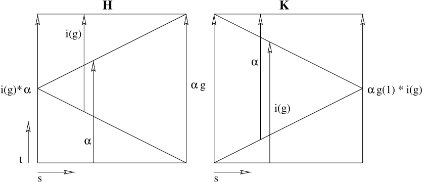
References

[1] M. F. Atiyah, R. Bott, and A. Shapiro, Clifford modules, Topology 3 (1964), 3–38, Supplement 1.
[2] S. J. Avis and C. J. Isham, Lorentz gauge invariant vacuum functionals for quantized spinor fields in non-simply connected space-times, Nucl. Phys. B156 (1979), 441–455.
[3] I. M. Benn and R. W. Tucker, An introduction to spinors and geometry with applications in physics, Adam Hilger, 1987.
[4] P. G. Bergmann, Two-component spinors in general relativity, Phys. Rev. 107 (1957), 624–629.
[5] H. J. Bernstein and A. V. Phillips, Fibre bundles and quantum theory, Scientific American 245 (1981), no. 1, 122–137.
[6] William M. Boothby, An introduction to differentiable manifolds and Riemannian geometry, second ed., Pure and Applied Mathematics, Academic Press, 1986.
[7] A. Borel, Sur la cohomologie des espaces fibrés principaux et des espaces homogènes de groupes de Lie compacts, Annals of Mathematics 57 (1953), 115–207.
[8] A. Borel and F. Hirzebruch, Characteristic classes and homogeneous spaces II, Amer. Journ. Math. 81 (1959), 315–382.
[9] E. Cartan, La theorie des groupes finis et continus et la geometrie differentielle : Traitees par la methode du repere mobile, Gauthier-Villars, 1951.
[10] Yvonne Choquet-Bruhat, Cécile de Witt-Morette, and Margaret Dillard-Bleick, Analysis, manifolds and physics, North Holland, 1977.
[11] C. J. S. Clarke, Magnetic charge, holonomy and characteristic classes: Illustrations of the methods of topology in relativity, General Relativity and Gravitation 2 (1971), no. 1, 43–51.
[12] R. H. Dalitz and R. Peierls, Biographical Memoirs of Fellows of the Royal Society, vol. 32, Royal Society, 1986, pp. 137–186.
[13] Cecile M. DeWitt and John A. Wheeler (eds.), Battelle rencontres, W. A. Benjamin, 1968.
[14] Jean A. Dieudonné, Treatise on analysis, vol. 3, Academic Press, 1972.
[15] by same author, Treatise on analysis, vol. 4, Academic Press, 1972.
[16] P. A. M. Dirac, The quantum theory of the electron, Proc. Roy. Soc. A117 (1928), 610–624.
[17] Samuel Eilenberg and Norman E. Steenrod, Foundations of algebraic topology, Princeton University Press, 1952.
[18] L. H. Ford, Vacuum polarization in a nonsimply connected space-time, Phys. Rev. D21 (1980), 933.
[19] William Fulton, Algebraic topology: a first course, Springer, 1995.
[20] Robert Geroch, Spinor structure of space-times in general relativity, I, Journal of Mathematical Physics 9 (1968), no. 11, 1739–1744.
[21] by same author, Spinor structure of space-times in general relativity, II, Journal of Mathematical Physics 11 (1970), no. 1, 343–348.
[22] S. W. Hawking and G. F. R. Ellis, The large scale structure of space-time, Cambridge University Press, 1973.
[23] Sigurdur Helgason, Differential geometry, Lie groups, and symmetric spaces, Academic Press, 1978.
[24] K. Hoffman and R. Kunze, Linear algebra, Prentice Hall, 1971.
[25] Sz. T. Hu, Homotopy theory, Academic Press, 1959.
[26] S. A. Huggett and K. P. Tod, An introduction to twistor theory, second ed., Cambridge University Press, 1994.
[27] Dale Husemoller, Fibre bundles, second ed., Springer-Verlag, 1966.
[28] Chris J. Isham, Spinor fields in four dimensional space-time, Proceedings of the Royal Society of London, A. 364 (1978), 591–599.
[29] by same author, Modern differential geometry for physicists, World Scientific, 1989.
[30] Anthony W. Knapp, Lie groups beyond an introduction, Birkhauser, 1996.
[31] Shoshichi Kobayashi and Katsumi Nomizu, Foundations of differential geometry, vol. 1, Interscience, 1963.
[32] by same author, Foundations of differential geometry, vol. 2, Interscience, 1969.
[33] H. Blaine Lawson, Jr and Marie-Louise Michelson, Spin geometry, Princeton University Press, 1989.
[34] André Lichnerowicz, Topics on space-times, in DeWitt and Wheeler [13], pp. 107–116.
[35] H. G. Liddell and R. Scott, A Greek–English lexicon, ninth revised ed., Clarendon, 1996.
[36] William S. Massey, Singular homology theory, Springer-Verlag, 1980.
[37] by same author, A basic course in algebraic topology, Springer, 1997.
[38] R. S. Millman and Ann K. Stehney, The geometry of connections, Am. Math. Soc. Monthly 80 (1973), 475–500.
[39] John W. Milnor, Spin structures on manifolds, L’enseignement math. 9 (1963), 198–203.
[40] by same author, Topology from the differentiable viewpoint, University Press of Virginia, 1965.
[41] Scott Morrison, An introduction to pull-backs of bundles and homotopy invariance, math.DG/0105161, August 2000.
[42] James R. Munkres, Topology: a first course, Prentice Hall, 1975.
[43] M. A. Naimark, Linear representations of the Lorentz Group, Pergamon, 1964.
[44] Barrett O’Neill, Semi-Riemannian geometry with applications to relativity, Academic Press, 1983.
[45] T. Parker and C. Taubes, On Witten’s proof of the positive energy theorem, Commun. Math. Phys. 84 (1982), 223–238.
[46] Roger Penrose, Structure of space-time, in DeWitt and Wheeler [13], pp. 121–235.
[47] Roger Penrose and Wolfgang Rindler, Spinors and space-time, vol. 1, Cambridge University Press, 1986.
[48] L. S. Pontryagin, Smooth manifolds and their applications in homotopy theory, Amer. Math. Soc. Translations 11 (1959), 1–144, Series 2. (Translated from Trudy Inst. Steklov 45 (1955)).
[49] Sylvan S. Schweber, An introduction to relativistic quantum field theory, Harper and Row, 1961.
[50] E. H. Spanier, Algebraic topology, McGraw Hill, 1966.
[51] Norman Steenrod, The topology of fibre bundles, Princeton University Press, 1951.
[52] Michael E. Taylor, Noncommutative harmonic analysis, American Mathematical Society, 1986.
[53] Robert M. Wald, General relativity, Chicago University Press, 1984.
[54] A. H. Wallace, Introduction to algebraic topology, Pergamon Press, 1957.
[55] E. Witten, A new proof of the positive energy theorem, Commun. Math. Phys. 80 (1981), 381–402.

	$\displaystyle(u_{\zeta}^{*}\omega)_{(m,\widetilde{e})}(v,X)$	$\displaystyle=\omega_{(m,\zeta(m))}(u_{\zeta*}(v,X))$
		$\displaystyle=\omega_{(m,\zeta(m))}(v,\zeta_{}v+\zeta(m)\rho_{e}X)$
		$\displaystyle=\omega_{(m,\zeta(m))}(v,0)+\omega_{(m,\zeta(m))}(0,\zeta_{}v+\zeta(m)\rho_{e}X)$
		$\displaystyle=\operatorname{Ad}(\zeta(m)^{-1})\omega_{(m,e)}(v,0)+\psi_{(m,\zeta(m))}(\zeta_{}v+\zeta(m)\rho_{*e}X)$
		$\displaystyle=\operatorname{Ad}(\zeta(m)^{-1})\omega_{(m,e)}(v,0)+\zeta(m)^{-1}\zeta_{}v+\rho_{e}X.$

Classifying Spinor Structures

Introduction

Conventions used throughout

Part I Geometry of Orthonormal Structures

1. The theory of principal fibre bundles

1.1. Fibre bundles

1.2. Principal fibre bundles

Definition 1.1.

Lemma 1.2.

Proof.

1.3. An example: the frame bundle of a manifold

2. Tensor algebras

2.1. Local tensor algebras

Example.

2.2. Associated vector bundles

2.3. General construction of a global tensor algebra

Example.

2.4. World tensors

2.5. Product bundles

Definition (Product bundle over a base space).

3. The special orthogonal groups

3.1. The indefinite inner product, and S​O​(p,q)𝑆𝑂𝑝𝑞SO(p,q) as a subgroup of G​L​(n,ℝ)𝐺𝐿𝑛ℝGL(n,\mathbb{R})

3.2. Index manipulations in the tensor algebra

3.3. Connected components

3.4. Lie algebras

4. Orthonormal structures: two viewpoints

4.1. Classical description of a metric tensor

Definition 4.1.

Definition.

4.2. Reduction to an orthogonal group

Definition.

4.3. Equivalence of these descriptions

4.4. The world tensor algebra for an orthonormal bundle

Proposition 4.2.

Proof.

4.5. The orthonormal bundle as a configuration space

5. Tensor calculus

5.1. Connection forms

Definition 5.1.

Proposition 5.2.

Proof.

Corollary.

Corollary.

5.2. Parallel transport

5.2.1. Horizontal lifting map

Lemma 5.3.

Proof.

5.2.2. Parallel transport

Proposition 5.4.

Proof.

5.2.3. Local representatives and Christoffel symbols

Proposition 5.5.

Proof.

5.2.4. Christoffel symbols for tensor product representations.

5.2.5. The difference between connections is a tensor

Proposition 5.6.

Proof.

5.2.6. Parallel transport in a local trivialisation

5.3. Covariant derivatives

5.4. Metric connections

Proposition 5.7.

5.4.1. An O​M𝑂𝑀OM connection is metric

Proposition 5.8.

Proof.

Corollary.

5.4.2. Metric connections are O​M𝑂𝑀OM connections

Part II Spinor Structure Classification

6. A preamble on covering spaces

6.1. Definitions

Definition 6.1.

Definition 6.2.

Proposition 6.3.

Proof.

Definition 6.4.

6.2. Paths and loops

Proposition 6.5.

Proof.

6.3. Fundamental groups

Proposition 6.6.

Proof.

3.1. The indefinite inner product, and $SO(p,q)$ as a subgroup of $GL(n,\mathbb{R})$

5.4.1. An $OM$ connection is metric

5.4.2. Metric connections are $OM$ connections