December 23, 2000

(Revised Edition)

ABSTRACT

We study the knot invariant based on the quantum dilogarithm function. This invariant can be regarded as a non-compact analogue of Kashaev’s invariant, or the colored Jones invariant, and is defined by an integral form. The 3-dimensional picture of our invariant originates from the pentagon identity of the quantum dilogarithm function, and we show that the hyperbolicity consistency conditions in gluing polyhedra arise naturally in the classical limit as the saddle point equation of our invariant.

Key Words:

1 Introduction

Since the discovery of the Jones polynomial [1], many knot invariants are proposed. In construction of these quantum invariants, the quantum group plays a crucial role, and a representation of the braid generator is derived from the universal $R$-matrix  [2]. Contrary to that the Alexander polynomial was known to be related with the homology of the universal abelian covering, the quantum invariants still lack the geometrical interpretation.

In Ref. 3, Kashaev introduced the knot invariant by use of the finite dimensional representation of the quantum dilogarithm function. He further conjectured [4] that the asymptotic behavior of this invariant for a hyperbolic knot $K$ gives the hyperbolic volume of the knot complement $S^{3}\setminus K$. As it is well known that the hyperbolic volume of the ideal tetrahedron is given by the Lobachevsky function [5, 6] which is closely related with the dilogarithm function, his conjecture may sound natural. Later in Ref. 7 Kashaev’s knot invariant was shown to be equivalent with the colored Jones polynomial at a specific value, and his conjecture is rewritten as the “volume conjecture”;

$$\|K\|=\frac{1}{v_{3}}\lim_{N\to\infty}\frac{2\,\pi}{N}\log|J_{N}(K)|,$$ (1.1)

where $\|K\|$ is the Gromov norm of $S^{3}\setminus K$, and $v_{3}$ is the hyperbolic volume of the regular ideal tetrahedron. The knot invariant $J_{N}(K)$ is defined from the colored Jones polynomial $V_{N}(K;t)$ ($N$-dimensional representation of $s\ell_{2}$) by

$$J_{N}(K)=V_{N}(K;\mathrm{e}^{\frac{2\,\pi\,\mathrm{i}}{N}}).$$

Thus to clarify a geometrical property of the quantum knot invariants such as the Jones polynomial, it is very fascinating to reveal the 3-dimensional picture of this invariant. Recently some geometrical aspects for the conjecture (1.1) have been proposed in Refs. 8 (see also Ref. [9]) based on the 3-dimensional picture of Ref. 10.

In this paper we define the knot invariant as a “non-compact” analogue of Kashaev’s invariant, or the colored Jones invariant. This is based on an infinite dimensional representation of the quantum dilogarithm function, and both the $R$-matrix and the invariant are defined in an integral form. In our construction a parameter $\gamma$ which corresponds to $\pi/N$ in eq. (1.1) is regarded as the Planck constant $\hbar/2$, and a limit in eq. (1.1) is realized by the classical limit $\gamma\to 0$. We shall demonstrate how the hyperbolic structure appears in the classical limit of the non-compact Jones invariant.

This paper is organized as follows. In § 2 we review the properties of the classical and quantum dilogarithm functions. A key is that both functions satisfy the so-called pentagon identity. Using these properties we construct a solution of the Yang–Baxter equation in terms of the quantum dilogarithm function. With this $R$-operator, we introduce the knot invariant in § 3. This invariant is given in the integral form from the beginning. We recall that the integral form of the quantum dilogarithm function was used in Ref. 4 to elucidate the asymptotic behavior of the colored Jones polynomial. In § 4 we show that the hyperbolic structure naturally appears in the classical limit of our knot invariant. We find that in $\gamma\to 0$ limit the oriented ideal tetrahedron with transverse oriented faces is associated to the matrix elements of the quantum dilogarithm function. Correspondingly the $R$-operator is identified with the oriented octahedron, whose vertices belong to the link $L$. This explains how the octahedron was introduced for each braiding in Ref. 10. We can apply the saddle point method to evaluate the asymptotic behavior of the classical limit of the knot invariant, and we further demonstrate that the saddle point equation for integrals of the knot invariant exactly coincides with the hyperbolicity consistency condition in gluing faces. Combining the fact that the imaginary part of the classical dilogarithm function gives the hyperbolic volume of the ideal tetrahedron at the critical point, we can conclude that the invariant is related with the hyperbolic volume of the knot complement at the critical point. In § 6 we show how to triangulate the knot complement in a case of the figure-eight knot. This method can be easily applied to other knots and links. The last section is devoted to discussions and concluding remarks.

2 Quantum Dilogarithm Function

2.1 Classical Dilogarithm Function

We collect properties concerning the classical dilogarithm function (see Refs. 11, 12 for review). The Euler dilogarithm function $\mathrm{Li}_{2}(x)$ is defined by

$$\mathrm{Li}_{2}(x)=\sum_{n=1}^{\infty}\frac{x^{n}}{n^{2}}=-\int_{0}^{x}\frac{\log(1-s)}{s}\,\mathrm{d}s.$$ (2.1)

The range $|x|\leq 1$ in an infinite series is extended outside the unit circle in the second integral form (2.1). We later use the Rogers dilogarithm function defined by

$$L(z)=\mathrm{Li}_{2}(z)+\frac{1}{2}\log z\,\log(1-z).$$ (2.2)

Based on the integral form of the dilogarithm function, we have the following identities (due to Euler);

$$\mathrm{Li}_{2}(z)+\mathrm{Li}_{2}(-z)=\frac{1}{2}\,\mathrm{Li}_{2}(z^{2}),$$ (2.3)

$$\mathrm{Li}_{2}(-z)+\mathrm{Li}_{2}(-z^{-1})=2\,\mathrm{Li}_{2}(-1)-\frac{1}{2}\bigl{(}\log z\bigr{)}^{2},$$ (2.4)

$$\mathrm{Li}_{2}(z)+\mathrm{Li}_{2}(1-z)=\mathrm{Li}_{2}(1)-\log z\,\log(1-z).$$ (2.5)

The first two identities are respectively called the duplication and inversion relations. By setting $z=\mathrm{e}^{\mathrm{i}\,\pi}$ in those identities, we get

$$\mathrm{Li}_{2}(1) =\frac{\pi^{2}}{6}, \mathrm{Li}_{2}(-1) =-\frac{\pi^{2}}{12}.$$ (2.6)

Besides above equations, we have a two-variable equation, which we call the pentagon identity (this form was first written by Schaeffer);

$$\mathrm{Li}_{2}(\frac{1-x^{-1}}{1-y^{-1}})=\mathrm{Li}_{2}(x)-\mathrm{Li}_{2}(y)+\mathrm{Li}_{2}(\frac{y}{x})+\mathrm{Li}_{2}(\frac{1-x}{1-y})-\frac{\pi^{2}}{6}+\log x\log(\frac{1-x}{1-y}),$$ (2.7)

or

$$L(x)-L(y)+L(\frac{y}{x})-L(\frac{1-x^{-1}}{1-y^{-1}})+L(\frac{1-x}{1-y})=\frac{\pi^{2}}{6}.$$ (2.8)

It is known that the variant of the dilogarithm function appears in the 3-dimensional hyperbolic geometry. Due to Refs. 5, 6, the volume of the ideal tetrahedron in the 3-dimensional hyperbolic space is given by the Bloch–Wigner function $D(z)$, which is defined by

$$D(z)=\text{Im}\,\mathrm{Li}_{2}(z)+\arg(1-z)\cdot\log|z|.$$ (2.9)

Here $z$ is a complex parameter $\text{Im}\,z>0$, which parameterizes the ideal tetrahedron; the Euclidean triangle cut out of any vertex of the ideal tetrahedron is similar to that in Fig. 1. From eq. (2.3)–(2.7) we get

$$D(z)=-D(z^{-1})=-D(1-z),$$ (2.10a)

$$D(x)-D(y)+D(\frac{y}{x})-D(\frac{1-x^{-1}}{1-y^{-1}})+D(\frac{1-x}{1-y})=0.$$ (2.10b)

Using the first identity we can extend a modulus $z$ to $z\in\mathbb{C}\setminus\{0,1\}$ by regarding $D(z)$ as the signed volume of the oriented tetrahedron.

Figure 1:

2.2 Quantum Dilogarithm Function and the $R$ Operator

We define a function $\Phi_{\gamma}(\varphi)$ by an integral form following Ref. 13:

$$\Phi_{\gamma}(\varphi)=\exp\left(\int_{\mathbb{R}+\mathrm{i}\,0}\frac{\mathrm{e}^{-\mathrm{i}\,\varphi\,x}}{4\operatorname{sh}(\gamma\,x)\,\operatorname{sh}(\pi\,x)}\,\frac{\mathrm{d}x}{x}\right),$$ (2.11)

where we take $\gamma\in\mathbb{R}$. We note that in Ref. 14 an essentially same integral was introduced in a context of the hyperbolic gamma function, and that in Ref. 15 another integral was studied as the quantum exponential function which solves the same functional equations below. Also the integral (2.11) was used to compute the asymptotic form of Kashaev’s invariant [4]. The function $\Phi_{\gamma}(\varphi)$ is known as a quantization of the dilogarithm function, and we have in a limit $\gamma\to 0$

$$\Phi_{\gamma}(\varphi)\sim\exp\left(\frac{1}{2\,\mathrm{i}\,\gamma}\,\mathrm{Li}_{2}(-\mathrm{e}^{\varphi})\right).$$ (2.12)

We list below several interesting properties of the integral $\Phi_{\gamma}(\varphi)$.

• Duality,

  $$\Phi_{\frac{\pi^{2}}{\gamma}}(\varphi)=\Phi_{\gamma}(\frac{\gamma}{\pi}\,\varphi).$$ (2.13)

• Zero points,

  $$\text{zeros of $\bigl{(}\Phi_{\gamma}(x)\bigr{)}^{\pm 1}$}=\Bigl{\{}\mp\mathrm{i}\,\bigl{(}(2\,m+1)\,\gamma+(2\,n+1)\,\pi\bigr{)}\ \big{|}\ m,n\in\mathbb{Z}_{\geq 0}\Bigr{\}}$$ (2.14)

• Inversion relation,

  $$\Phi_{\gamma}(x)\cdot\Phi_{\gamma}(-x)=\exp\left(-\frac{1}{2\,\mathrm{i}\,\gamma}\Bigl{(}\frac{x^{2}}{2}+\frac{\pi^{2}+\gamma^{2}}{6}\Bigr{)}\right).$$ (2.15)

  By taking a limit $\gamma\to 0$ and using eq. (2.12), we obtain

  $$\mathrm{Li}_{2}(-\mathrm{e}^{x})+\mathrm{Li}_{2}(-\mathrm{e}^{-x})+\frac{x^{2}}{2}+\frac{\pi^{2}}{6}=0,$$

  which is nothing but the inversion identity (2.4) for the Euler dilogarithm function.

• Difference equations,

  $$\frac{\Phi_{\gamma}(\varphi+\mathrm{i}\,\gamma)}{\Phi_{\gamma}(\varphi-\mathrm{i}\,\gamma)} =\frac{1}{1+\mathrm{e}^{\varphi}},$$ (2.16a)

  $$\frac{\Phi_{\gamma}(\varphi+\mathrm{i}\,\pi)}{\Phi_{\gamma}(\varphi-\mathrm{i}\,\pi)} =\frac{1}{1+\mathrm{e}^{\frac{\pi}{\gamma}\varphi}}.$$ (2.16b)

• Pentagon relation [16, 17, 18],

  $$\Phi_{\gamma}(\hat{p})\,\Phi_{\gamma}(\hat{q})=\Phi_{\gamma}(\hat{q})\,\Phi_{\gamma}(\hat{p}+\hat{q})\,\Phi_{\gamma}(\hat{p}),$$ (2.17)

  where $\hat{p}$ and $\hat{q}$ are the canonically conjugate operators satisfying the Heisenberg commutation relation,

  $$[\hat{p}~{},~{}\hat{q}]=-2\,\mathrm{i}\,\gamma.$$ (2.18)

  In this sense, the parameter $\gamma$ in the integral (2.11) is the Planck constant.

• The Fourier transformation [19, 20],

  $$\frac{1}{\sqrt{4\,\pi\,\gamma}}\int\mathrm{d}y\ \Phi_{\gamma}(y)\,\mathrm{e}^{\frac{1}{2\,\mathrm{i}\,\gamma}\,x\,y}=\Phi_{\gamma}(-x+\mathrm{i}\pi+\mathrm{i}\gamma)\,\mathrm{e}^{\frac{1}{2\,\mathrm{i}\,\gamma}\left(\frac{x^{2}}{2}-\frac{1}{2}\pi\gamma-\frac{\pi^{2}+\gamma^{2}}{6}\right)},$$ (2.19a)

  $$\frac{1}{\sqrt{4\,\pi\,\gamma}}\int\mathrm{d}y\ \frac{1}{\Phi_{\gamma}(y)}\,\mathrm{e}^{\frac{1}{2\,\mathrm{i}\,\gamma}x\,y}=\frac{1}{\Phi_{\gamma}(x-\mathrm{i}\,\pi-\mathrm{i}\,\gamma)}\,\mathrm{e}^{-\frac{1}{2\,\mathrm{i}\,\gamma}\left(\frac{x^{2}}{2}-\frac{1}{2}\pi\gamma-\frac{\pi^{2}+\gamma^{2}}{6}\right)},$$ (2.19b)

  $$\begin{split}&\frac{1}{\sqrt{4\,\pi\,\gamma}}\int\mathrm{d}y\ \frac{\Phi_{\gamma}(y+u)}{\Phi_{\gamma}(y+v)}\,\mathrm{e}^{-\frac{1}{2\mathrm{i}\gamma}\,x\,y}\\ &\qquad=\frac{\Phi_{\gamma}(v-u-x+\mathrm{i}\pi+\mathrm{i}\gamma)}{\Phi_{\gamma}(v-u+\mathrm{i}\pi+\mathrm{i}\gamma)\,\Phi_{\gamma}(-x-\mathrm{i}\pi-\mathrm{i}\gamma)}\,\mathrm{e}^{\frac{1}{2\mathrm{i}\gamma}\left(x(u-\mathrm{i}\pi-\mathrm{i}\gamma)+\frac{1}{2}\pi\gamma+\frac{\pi^{2}+\gamma^{2}}{6}\right)}.\end{split}$$ (2.19c)

For our later convention, we rewrite the pentagon identity (2.17) into a simple form. We define the $S$-operator on $\mathbf{V}\otimes\mathbf{V}$ by

$$S_{1,2}=\mathrm{e}^{\frac{1}{2\,\mathrm{i}\,\gamma}\,\hat{q}_{1}\,\hat{p}_{2}}\,\Phi_{\gamma}(\hat{p}_{1}+\hat{q}_{2}-\hat{p}_{2}),$$ (2.20)

where the Heisenberg operators $\hat{p}_{a}$ and $\hat{q}_{a}$ act on the $a$-th vector space $\mathbf{V}$. Then the pentagon identity (2.17) can be rewritten as

$$S_{2,3}\,S_{1,2}=S_{1,2}\,S_{1,3}\,S_{2,3},$$ (2.21)

where $S_{a,b}$ acts on the $a$- and $b$-th spaces of $\mathbf{V}\otimes\mathbf{V}\otimes\mathbf{V}$. See that the operator, $T_{1,2}=\mathrm{e}^{\frac{1}{2\,\mathrm{i}\,\gamma}\,\hat{q}_{1}\,\hat{p}_{2}}$, which is a prefactor of the $S$-operator (2.20), is a simple solution of eq. (2.21). We remark that the pentagon identity (2.21) is a natural consequence of the Heisenberg double [21, 22], in which the $S$-operator is given by

$$S=\sum_{\alpha}e_{\alpha}\otimes e^{\alpha}.$$

Here $\{e_{\alpha},e^{\alpha}\}$ is a set of generators satisfying

$$e_{\alpha}\,e_{\beta}=\sum_{\gamma}m^{\gamma}_{\alpha~{}\beta}\,e_{\gamma},$$

$$e^{\alpha}\,e^{\beta}=\sum_{\gamma}\mu_{\gamma}^{\alpha~{}\beta}\,e^{\gamma},$$

$$e_{\alpha}\,e^{\beta}=\sum_{\gamma,\rho,\sigma}m^{\beta}_{\rho~{}\gamma}\,\mu_{\alpha}^{\gamma~{}\sigma}\,e^{\rho}\,e_{\sigma}.$$

For our purpose to define the knot invariant, we introduce the $R$-operator by use of the $S$-operators as [18, 21, 23]

$$R_{12,34}=\Bigl{(}S_{1,4}^{\mathrm{t}_{4}}\Bigr{)}^{-1}\,S_{1,3}\,S_{2,4}^{\mathrm{t}_{2}\mathrm{t}_{4}}\,\Bigl{(}S_{2,3}^{\mathrm{t}_{2}}\Bigr{)}^{-1},$$ (2.22)

and we set

$$\check{R}_{12,34}=P_{1,3}\,P_{2,4}\,R_{12,34}.$$ (2.23)

Here $\mathrm{t}_{a}$ means a transposition on the $a$-th space, and $P$ is the permutation operator. The $R$-operator acts on a vector space $\mathbf{V}^{\otimes 4}$. Based on the pentagon identity (2.21), we find that the $\check{R}$-operator (2.23) satisfies the Yang–Baxter relation,

$$\check{R}_{11^{\prime},22^{\prime}}\,\check{R}_{22^{\prime},33^{\prime}}\,\check{R}_{11^{\prime},22^{\prime}}=\check{R}_{22^{\prime},33^{\prime}}\,\check{R}_{11^{\prime},22^{\prime}}\,\check{R}_{22^{\prime},33^{\prime}}.$$ (2.24)

By regarding the $R$-operator as an operator on $\mathbf{W}\otimes\mathbf{W}$ with $\mathbf{W}=\mathbf{V}^{\otimes 2}$, this Yang–Baxter relation can be seen as a braid relation as usual, which can be depicted as a projection onto 2-dimensional space in Fig. 2.

$$\lx@xy@svg{\hbox{\raise 0.0pt\hbox{\kern 24.0pt\hbox{\ignorespaces\ignorespaces\ignorespaces\ignorespaces\ignorespaces\ignorespaces\ignorespaces\ignorespaces\ignorespaces\ignorespaces\ignorespaces\ignorespaces\ignorespaces\ignorespaces\ignorespaces\ignorespaces\ignorespaces\ignorespaces\ignorespaces\ignorespaces\ignorespaces\ignorespaces\ignorespaces\ignorespaces\ignorespaces\ignorespaces\ignorespaces\ignorespaces\ignorespaces\ignorespaces\ignorespaces{}{}{}{{}}{}\ignorespaces\ignorespaces\hbox{\hbox{\kern 0.0pt\raise 0.0pt\hbox{{}{}{}{{}{}{}}{}}}}\ignorespaces{}\ignorespaces{}{}{}{{}{}}{\hbox{\kern 9.5pt\raise 36.0pt\hbox{\hbox{\kern 0.0pt\raise 0.0pt\hbox{$\scriptstyle{\hbox to5.0pt{\hfill\vrule height=2.5pt,depth=2.5pt,width=0.0pt}}$}}}}}\ignorespaces\ignorespaces\hbox{\hbox{\kern 0.0pt\raise 0.0pt\hbox{{}{}{}{{}{}{}{{{}}{{}}{{}}{{}}{{}}{{}}{{}}{{}}{{}}{{}}{{}}{{}}{{}}{{}}{{}}{{}}{}{{}}{{}}{{}}{{}}{{}}{{}}{{}}{{}}{{}}{{}}{{}}{{}}{{}}{{}}{{}}{{}}{{}}{{}}{{}}{{}}{{}}{{}}{{}}{{}}{{}}{{}}{{}}{}}}{{}{}{}\lx@xy@spline@}{}}}}\ignorespaces{}\ignorespaces{}{}{}{{}}{}\ignorespaces\ignorespaces\hbox{\hbox{\kern 0.0pt\raise 0.0pt\hbox{{}{{}{}{}{{{}}{{}}{}{{}}{{}}{{}}{{}}{{}}{{}}{{}}{{}}{{}}{{}}{{}}{{}}{{}}{{}}{{}}{{}}{{}}{{}}}}{}{}{{}{}{}\lx@xy@spline@}{}}}}\ignorespaces{}\ignorespaces\hbox{\hbox{\kern 0.0pt\raise 0.0pt\hbox{{}{}{}{{}{}{}}{}}}}\ignorespaces{}\ignorespaces\ignorespaces\ignorespaces\ignorespaces\ignorespaces\ignorespaces\ignorespaces\ignorespaces\ignorespaces{}{}{}{{}}{}\ignorespaces\ignorespaces\hbox{\hbox{\kern 0.0pt\raise 0.0pt\hbox{{}{}{}{{}{}{}}{}}}}\ignorespaces{}\ignorespaces{}{}{}{{}}{}\ignorespaces\ignorespaces\hbox{\hbox{\kern 0.0pt\raise 0.0pt\hbox{{}{}{}{}{{}{}{}\lx@xy@spline@}{}}}}\ignorespaces{}\ignorespaces\hbox{\hbox{\kern 0.0pt\raise 0.0pt\hbox{{}{}{}{{}{}{}}{}}}}\ignorespaces{}\ignorespaces\ignorespaces\ignorespaces\ignorespaces\ignorespaces\ignorespaces\ignorespaces\ignorespaces\ignorespaces\ignorespaces\ignorespaces\ignorespaces\ignorespaces\ignorespaces\ignorespaces\ignorespaces\ignorespaces\ignorespaces\ignorespaces\ignorespaces\ignorespaces\ignorespaces\ignorespaces\ignorespaces\ignorespaces\ignorespaces\ignorespaces\ignorespaces\ignorespaces{}{}{}{{}}{}\ignorespaces\ignorespaces\hbox{\hbox{\kern 0.0pt\raise 0.0pt\hbox{{}{}{}{{}{}{}}{}}}}\ignorespaces{}\ignorespaces{}{}{}{{}}{}\ignorespaces\ignorespaces\hbox{\hbox{\kern 0.0pt\raise 0.0pt\hbox{{}{}{}{}{{}{}{}\lx@xy@spline@}{}}}}\ignorespaces{}\ignorespaces\hbox{\hbox{\kern 0.0pt\raise 0.0pt\hbox{{}{}{}{{}{}{}}{}}}}\ignorespaces{}\ignorespaces\ignorespaces\ignorespaces\ignorespaces\ignorespaces\ignorespaces\ignorespaces\ignorespaces\ignorespaces\ignorespaces\ignorespaces\ignorespaces\ignorespaces\ignorespaces\ignorespaces\ignorespaces\ignorespaces\ignorespaces\ignorespaces\ignorespaces\ignorespaces\ignorespaces\ignorespaces\ignorespaces\ignorespaces\ignorespaces\ignorespaces\ignorespaces\ignorespaces\ignorespaces\ignorespaces\ignorespaces\ignorespaces{}{}{}{{}}{}\ignorespaces\ignorespaces\hbox{\hbox{\kern 0.0pt\raise 0.0pt\hbox{{}{}{}{{}{}{}}{}}}}\ignorespaces{}\ignorespaces{}{}{}{{}}{}\ignorespaces\ignorespaces\hbox{\hbox{\kern 0.0pt\raise 0.0pt\hbox{{}{}{}{}{{}{}{}\lx@xy@spline@}{}}}}\ignorespaces{}\ignorespaces\hbox{\hbox{\kern 0.0pt\raise 0.0pt\hbox{{}{}{}{{}{}{}}{}}}}\ignorespaces{}\ignorespaces\ignorespaces\ignorespaces\ignorespaces\ignorespaces\ignorespaces\ignorespaces\ignorespaces\ignorespaces\ignorespaces\ignorespaces\ignorespaces\ignorespaces\ignorespaces\ignorespaces\ignorespaces\ignorespaces\ignorespaces\ignorespaces\ignorespaces\ignorespaces\ignorespaces\ignorespaces\ignorespaces\ignorespaces\ignorespaces\ignorespaces\ignorespaces{}{}{}{{}}{}\ignorespaces\ignorespaces\hbox{\hbox{\kern 0.0pt\raise 0.0pt\hbox{{}{}{}{{}{}{}}{}}}}\ignorespaces{}\ignorespaces{}{}{}{{}{}}{\hbox{\kern 33.5pt\raise 0.0pt\hbox{\hbox{\kern 0.0pt\raise 0.0pt\hbox{$\scriptstyle{\hbox to5.0pt{\hfill\vrule height=2.5pt,depth=2.5pt,width=0.0pt}}$}}}}}\ignorespaces\ignorespaces\hbox{\hbox{\kern 0.0pt\raise 0.0pt\hbox{{}{}{}{{}{}{}{{{}}{{}}{{}}{{}}{{}}{{}}{{}}{{}}{{}}{{}}{{}}{{}}{{}}{{}}{{}}{{}}{}{{}}{{}}{{}}{{}}{{}}{{}}{{}}{{}}{{}}{{}}{{}}{{}}{{}}{{}}{{}}{{}}{{}}{{}}{{}}{{}}{{}}{{}}{{}}{{}}{{}}{{}}{{}}{}}}{{}{}{}\lx@xy@spline@}{}}}}\ignorespaces{}\ignorespaces{}{}{}{{}}{}\ignorespaces\ignorespaces\hbox{\hbox{\kern 0.0pt\raise 0.0pt\hbox{{}{{}{}{}{{{}}{{}}{}{{}}{{}}{{}}{{}}{{}}{{}}{{}}{{}}{{}}{{}}{{}}{{}}{{}}{{}}{{}}{{}}{{}}{{}}}}{}{}{{}{}{}\lx@xy@spline@}{}}}}\ignorespaces{}\ignorespaces\hbox{\hbox{\kern 0.0pt\raise 0.0pt\hbox{{}{}{}{{}{}{}}{}}}}\ignorespaces{}\ignorespaces\ignorespaces\ignorespaces\ignorespaces\ignorespaces\ignorespaces\ignorespaces\ignorespaces\ignorespaces{}{}{}{{}}{}\ignorespaces\ignorespaces\hbox{\hbox{\kern 0.0pt\raise 0.0pt\hbox{{}{}{}{{}{}{}}{}}}}\ignorespaces{}\ignorespaces{}{}{}{{}}{}\ignorespaces\ignorespaces\hbox{\hbox{\kern 0.0pt\raise 0.0pt\hbox{{}{}{}{}{{}{}{}\lx@xy@spline@}{}}}}\ignorespaces{}\ignorespaces\hbox{\hbox{\kern 0.0pt\raise 0.0pt\hbox{{}{}{}{{}{}{}}{}}}}\ignorespaces{}\ignorespaces\ignorespaces\ignorespaces\ignorespaces\ignorespaces\ignorespaces\ignorespaces\ignorespaces\ignorespaces\ignorespaces\ignorespaces\ignorespaces\ignorespaces\ignorespaces\ignorespaces\ignorespaces\ignorespaces\ignorespaces\ignorespaces\ignorespaces\ignorespaces\ignorespaces\ignorespaces\ignorespaces\ignorespaces\ignorespaces\ignorespaces\ignorespaces\ignorespaces\ignorespaces{}{}{}{{}}{}\ignorespaces\ignorespaces\hbox{\hbox{\kern 0.0pt\raise 0.0pt\hbox{{}{}{}{{}{}{}}{}}}}\ignorespaces{}\ignorespaces{}{}{}{{}{}}{\hbox{\kern 9.5pt\raise-36.0pt\hbox{\hbox{\kern 0.0pt\raise 0.0pt\hbox{$\scriptstyle{\hbox to5.0pt{\hfill\vrule height=2.5pt,depth=2.5pt,width=0.0pt}}$}}}}}\ignorespaces\ignorespaces\hbox{\hbox{\kern 0.0pt\raise 0.0pt\hbox{{}{}{}{{}{}{}{{{}}{{}}{{}}{{}}{{}}{{}}{{}}{{}}{{}}{{}}{{}}{{}}{{}}{{}}{{}}{{}}{}{{}}{{}}{{}}{{}}{{}}{{}}{{}}{{}}{{}}{{}}{{}}{{}}{{}}{{}}{{}}{{}}{{}}{{}}{{}}{{}}{{}}{{}}{{}}{{}}{{}}{{}}{{}}{}}}{{}{}{}\lx@xy@spline@}{}}}}\ignorespaces{}\ignorespaces{}{}{}{{}}{}\ignorespaces\ignorespaces\hbox{\hbox{\kern 0.0pt\raise 0.0pt\hbox{{}{{}{}{}{{{}}{{}}{}{{}}{{}}{{}}{{}}{{}}{{}}{{}}{{}}{{}}{{}}{{}}{{}}{{}}{{}}{{}}{{}}{{}}{{}}}}{}{}{{}{}{}\lx@xy@spline@}{}}}}\ignorespaces{}\ignorespaces\hbox{\hbox{\kern 0.0pt\raise 0.0pt\hbox{{}{}{}{{}{}{}}{}}}}\ignorespaces{}\ignorespaces\ignorespaces\ignorespaces\ignorespaces\ignorespaces\ignorespaces\ignorespaces\ignorespaces\ignorespaces{}{}{}{{}}{}\ignorespaces\ignorespaces\hbox{\hbox{\kern 0.0pt\raise 0.0pt\hbox{{}{}{}{{}{}{}}{}}}}\ignorespaces{}\ignorespaces{}{}{}{{}}{}\ignorespaces\ignorespaces\hbox{\hbox{\kern 0.0pt\raise 0.0pt\hbox{{}{}{}{}{{}{}{}\lx@xy@spline@}{}}}}\ignorespaces{}\ignorespaces\hbox{\hbox{\kern 0.0pt\raise 0.0pt\hbox{{}{}{}{{}{}{}}{}}}}\ignorespaces{}\ignorespaces\ignorespaces\ignorespaces\ignorespaces\ignorespaces\ignorespaces\ignorespaces\ignorespaces\ignorespaces\ignorespaces\ignorespaces\ignorespaces\ignorespaces\ignorespaces\ignorespaces\ignorespaces\ignorespaces\ignorespaces\ignorespaces\ignorespaces\ignorespaces\ignorespaces\ignorespaces\ignorespaces\ignorespaces\ignorespaces\ignorespaces\ignorespaces\ignorespaces{}{}{}{{}}{}\ignorespaces\ignorespaces\hbox{\hbox{\kern 0.0pt\raise 0.0pt\hbox{{}{}{}{{}{}{}}{}}}}\ignorespaces{}\ignorespaces{}{}{}{{}}{}\ignorespaces\ignorespaces\hbox{\hbox{\kern 0.0pt\raise 0.0pt\hbox{{}{}{}{}{{}{}{}\lx@xy@spline@}{}}}}\ignorespaces{}\ignorespaces\hbox{\hbox{\kern 0.0pt\raise 0.0pt\hbox{{}{}{}{{}{}{}}{}}}}\ignorespaces{}\ignorespaces\ignorespaces\ignorespaces{}}}}}\ignorespaces=\lx@xy@svg{\hbox{\raise 0.0pt\hbox{\kern 24.0pt\hbox{\ignorespaces\ignorespaces\ignorespaces\ignorespaces\ignorespaces\ignorespaces\ignorespaces\ignorespaces\ignorespaces\ignorespaces\ignorespaces\ignorespaces\ignorespaces\ignorespaces\ignorespaces\ignorespaces\ignorespaces\ignorespaces\ignorespaces\ignorespaces\ignorespaces\ignorespaces\ignorespaces\ignorespaces\ignorespaces\ignorespaces\ignorespaces\ignorespaces\ignorespaces\ignorespaces\ignorespaces\ignorespaces\ignorespaces\ignorespaces{}{}{}{{}}{}\ignorespaces\ignorespaces\hbox{\hbox{\kern 0.0pt\raise 0.0pt\hbox{{}{}{}{{}{}{}}{}}}}\ignorespaces{}\ignorespaces{}{}{}{{}}{}\ignorespaces\ignorespaces\hbox{\hbox{\kern 0.0pt\raise 0.0pt\hbox{{}{}{}{}{{}{}{}\lx@xy@spline@}{}}}}\ignorespaces{}\ignorespaces\hbox{\hbox{\kern 0.0pt\raise 0.0pt\hbox{{}{}{}{{}{}{}}{}}}}\ignorespaces{}\ignorespaces\ignorespaces\ignorespaces\ignorespaces\ignorespaces\ignorespaces\ignorespaces\ignorespaces\ignorespaces\ignorespaces\ignorespaces\ignorespaces\ignorespaces\ignorespaces\ignorespaces\ignorespaces\ignorespaces\ignorespaces\ignorespaces\ignorespaces\ignorespaces\ignorespaces\ignorespaces\ignorespaces\ignorespaces\ignorespaces\ignorespaces\ignorespaces{}{}{}{{}}{}\ignorespaces\ignorespaces\hbox{\hbox{\kern 0.0pt\raise 0.0pt\hbox{{}{}{}{{}{}{}}{}}}}\ignorespaces{}\ignorespaces{}{}{}{{}{}}{\hbox{\kern 33.5pt\raise 36.0pt\hbox{\hbox{\kern 0.0pt\raise 0.0pt\hbox{$\scriptstyle{\hbox to5.0pt{\hfill\vrule height=2.5pt,depth=2.5pt,width=0.0pt}}$}}}}}\ignorespaces\ignorespaces\hbox{\hbox{\kern 0.0pt\raise 0.0pt\hbox{{}{}{}{{}{}{}{{{}}{{}}{{}}{{}}{{}}{{}}{{}}{{}}{{}}{{}}{{}}{{}}{{}}{{}}{{}}{{}}{}{{}}{{}}{{}}{{}}{{}}{{}}{{}}{{}}{{}}{{}}{{}}{{}}{{}}{{}}{{}}{{}}{{}}{{}}{{}}{{}}{{}}{{}}{{}}{{}}{{}}{{}}{{}}{}}}{{}{}{}\lx@xy@spline@}{}}}}\ignorespaces{}\ignorespaces{}{}{}{{}}{}\ignorespaces\ignorespaces\hbox{\hbox{\kern 0.0pt\raise 0.0pt\hbox{{}{{}{}{}{{{}}{{}}{}{{}}{{}}{{}}{{}}{{}}{{}}{{}}{{}}{{}}{{}}{{}}{{}}{{}}{{}}{{}}{{}}{{}}{{}}}}{}{}{{}{}{}\lx@xy@spline@}{}}}}\ignorespaces{}\ignorespaces\hbox{\hbox{\kern 0.0pt\raise 0.0pt\hbox{{}{}{}{{}{}{}}{}}}}\ignorespaces{}\ignorespaces\ignorespaces\ignorespaces\ignorespaces\ignorespaces\ignorespaces\ignorespaces\ignorespaces\ignorespaces{}{}{}{{}}{}\ignorespaces\ignorespaces\hbox{\hbox{\kern 0.0pt\raise 0.0pt\hbox{{}{}{}{{}{}{}}{}}}}\ignorespaces{}\ignorespaces{}{}{}{{}}{}\ignorespaces\ignorespaces\hbox{\hbox{\kern 0.0pt\raise 0.0pt\hbox{{}{}{}{}{{}{}{}\lx@xy@spline@}{}}}}\ignorespaces{}\ignorespaces\hbox{\hbox{\kern 0.0pt\raise 0.0pt\hbox{{}{}{}{{}{}{}}{}}}}\ignorespaces{}\ignorespaces\ignorespaces\ignorespaces\ignorespaces\ignorespaces\ignorespaces\ignorespaces\ignorespaces\ignorespaces\ignorespaces\ignorespaces\ignorespaces\ignorespaces\ignorespaces\ignorespaces\ignorespaces\ignorespaces\ignorespaces\ignorespaces\ignorespaces\ignorespaces\ignorespaces\ignorespaces\ignorespaces\ignorespaces\ignorespaces\ignorespaces\ignorespaces\ignorespaces\ignorespaces{}{}{}{{}}{}\ignorespaces\ignorespaces\hbox{\hbox{\kern 0.0pt\raise 0.0pt\hbox{{}{}{}{{}{}{}}{}}}}\ignorespaces{}\ignorespaces{}{}{}{{}{}}{\hbox{\kern 9.5pt\raise 0.0pt\hbox{\hbox{\kern 0.0pt\raise 0.0pt\hbox{$\scriptstyle{\hbox to5.0pt{\hfill\vrule height=2.5pt,depth=2.5pt,width=0.0pt}}$}}}}}\ignorespaces\ignorespaces\hbox{\hbox{\kern 0.0pt\raise 0.0pt\hbox{{}{}{}{{}{}{}{{{}}{{}}{{}}{{}}{{}}{{}}{{}}{{}}{{}}{{}}{{}}{{}}{{}}{{}}{{}}{{}}{}{{}}{{}}{{}}{{}}{{}}{{}}{{}}{{}}{{}}{{}}{{}}{{}}{{}}{{}}{{}}{{}}{{}}{{}}{{}}{{}}{{}}{{}}{{}}{{}}{{}}{{}}{{}}{}}}{{}{}{}\lx@xy@spline@}{}}}}\ignorespaces{}\ignorespaces{}{}{}{{}}{}\ignorespaces\ignorespaces\hbox{\hbox{\kern 0.0pt\raise 0.0pt\hbox{{}{{}{}{}{{{}}{{}}{}{{}}{{}}{{}}{{}}{{}}{{}}{{}}{{}}{{}}{{}}{{}}{{}}{{}}{{}}{{}}{{}}{{}}{{}}}}{}{}{{}{}{}\lx@xy@spline@}{}}}}\ignorespaces{}\ignorespaces\hbox{\hbox{\kern 0.0pt\raise 0.0pt\hbox{{}{}{}{{}{}{}}{}}}}\ignorespaces{}\ignorespaces\ignorespaces\ignorespaces\ignorespaces\ignorespaces\ignorespaces\ignorespaces\ignorespaces\ignorespaces{}{}{}{{}}{}\ignorespaces\ignorespaces\hbox{\hbox{\kern 0.0pt\raise 0.0pt\hbox{{}{}{}{{}{}{}}{}}}}\ignorespaces{}\ignorespaces{}{}{}{{}}{}\ignorespaces\ignorespaces\hbox{\hbox{\kern 0.0pt\raise 0.0pt\hbox{{}{}{}{}{{}{}{}\lx@xy@spline@}{}}}}\ignorespaces{}\ignorespaces\hbox{\hbox{\kern 0.0pt\raise 0.0pt\hbox{{}{}{}{{}{}{}}{}}}}\ignorespaces{}\ignorespaces\ignorespaces\ignorespaces\ignorespaces\ignorespaces\ignorespaces\ignorespaces\ignorespaces\ignorespaces\ignorespaces\ignorespaces\ignorespaces\ignorespaces\ignorespaces\ignorespaces\ignorespaces\ignorespaces\ignorespaces\ignorespaces\ignorespaces\ignorespaces\ignorespaces\ignorespaces\ignorespaces\ignorespaces\ignorespaces\ignorespaces\ignorespaces\ignorespaces{}{}{}{{}}{}\ignorespaces\ignorespaces\hbox{\hbox{\kern 0.0pt\raise 0.0pt\hbox{{}{}{}{{}{}{}}{}}}}\ignorespaces{}\ignorespaces{}{}{}{{}}{}\ignorespaces\ignorespaces\hbox{\hbox{\kern 0.0pt\raise 0.0pt\hbox{{}{}{}{}{{}{}{}\lx@xy@spline@}{}}}}\ignorespaces{}\ignorespaces\hbox{\hbox{\kern 0.0pt\raise 0.0pt\hbox{{}{}{}{{}{}{}}{}}}}\ignorespaces{}\ignorespaces\ignorespaces\ignorespaces\ignorespaces\ignorespaces\ignorespaces\ignorespaces\ignorespaces\ignorespaces\ignorespaces\ignorespaces\ignorespaces\ignorespaces\ignorespaces\ignorespaces\ignorespaces\ignorespaces\ignorespaces\ignorespaces\ignorespaces\ignorespaces\ignorespaces\ignorespaces\ignorespaces\ignorespaces\ignorespaces\ignorespaces\ignorespaces\ignorespaces\ignorespaces\ignorespaces\ignorespaces\ignorespaces{}{}{}{{}}{}\ignorespaces\ignorespaces\hbox{\hbox{\kern 0.0pt\raise 0.0pt\hbox{{}{}{}{{}{}{}}{}}}}\ignorespaces{}\ignorespaces{}{}{}{{}}{}\ignorespaces\ignorespaces\hbox{\hbox{\kern 0.0pt\raise 0.0pt\hbox{{}{}{}{}{{}{}{}\lx@xy@spline@}{}}}}\ignorespaces{}\ignorespaces\hbox{\hbox{\kern 0.0pt\raise 0.0pt\hbox{{}{}{}{{}{}{}}{}}}}\ignorespaces{}\ignorespaces\ignorespaces\ignorespaces\ignorespaces\ignorespaces\ignorespaces\ignorespaces\ignorespaces\ignorespaces\ignorespaces\ignorespaces\ignorespaces\ignorespaces\ignorespaces\ignorespaces\ignorespaces\ignorespaces\ignorespaces\ignorespaces\ignorespaces\ignorespaces\ignorespaces\ignorespaces\ignorespaces\ignorespaces\ignorespaces\ignorespaces\ignorespaces{}{}{}{{}}{}\ignorespaces\ignorespaces\hbox{\hbox{\kern 0.0pt\raise 0.0pt\hbox{{}{}{}{{}{}{}}{}}}}\ignorespaces{}\ignorespaces{}{}{}{{}{}}{\hbox{\kern 33.5pt\raise-36.0pt\hbox{\hbox{\kern 0.0pt\raise 0.0pt\hbox{$\scriptstyle{\hbox to5.0pt{\hfill\vrule height=2.5pt,depth=2.5pt,width=0.0pt}}$}}}}}\ignorespaces\ignorespaces\hbox{\hbox{\kern 0.0pt\raise 0.0pt\hbox{{}{}{}{{}{}{}{{{}}{{}}{{}}{{}}{{}}{{}}{{}}{{}}{{}}{{}}{{}}{{}}{{}}{{}}{{}}{{}}{}{{}}{{}}{{}}{{}}{{}}{{}}{{}}{{}}{{}}{{}}{{}}{{}}{{}}{{}}{{}}{{}}{{}}{{}}{{}}{{}}{{}}{{}}{{}}{{}}{{}}{{}}{{}}{}}}{{}{}{}\lx@xy@spline@}{}}}}\ignorespaces{}\ignorespaces{}{}{}{{}}{}\ignorespaces\ignorespaces\hbox{\hbox{\kern 0.0pt\raise 0.0pt\hbox{{}{{}{}{}{{{}}{{}}{}{{}}{{}}{{}}{{}}{{}}{{}}{{}}{{}}{{}}{{}}{{}}{{}}{{}}{{}}{{}}{{}}{{}}{{}}}}{}{}{{}{}{}\lx@xy@spline@}{}}}}\ignorespaces{}\ignorespaces\hbox{\hbox{\kern 0.0pt\raise 0.0pt\hbox{{}{}{}{{}{}{}}{}}}}\ignorespaces{}\ignorespaces\ignorespaces\ignorespaces\ignorespaces\ignorespaces\ignorespaces\ignorespaces\ignorespaces\ignorespaces{}{}{}{{}}{}\ignorespaces\ignorespaces\hbox{\hbox{\kern 0.0pt\raise 0.0pt\hbox{{}{}{}{{}{}{}}{}}}}\ignorespaces{}\ignorespaces{}{}{}{{}}{}\ignorespaces\ignorespaces\hbox{\hbox{\kern 0.0pt\raise 0.0pt\hbox{{}{}{}{}{{}{}{}\lx@xy@spline@}{}}}}\ignorespaces{}\ignorespaces\hbox{\hbox{\kern 0.0pt\raise 0.0pt\hbox{{}{}{}{{}{}{}}{}}}}\ignorespaces{}\ignorespaces\ignorespaces\ignorespaces{}}}}}\ignorespaces$$

Figure 2: Braid relation, or the constant Yang–Baxter equation.

2.3 Representation

We now give the representation of these operators on the momentum space; $\hat{p}\,|p\rangle=p\,|p\rangle$ with $p\in\mathbb{R}$, and we take the vector space as $\mathbf{V}=L^{2}(\mathbb{R})$. The matrix elements of the $S$-operators are given by [23]

$$\langle p_{1},p_{2}\ |\ S_{1,2}\ |\ p_{1}^{\prime},p_{2}^{\prime}\rangle =\frac{1}{4\,\pi\,\gamma}\,\delta(p_{1}+p_{2}-p_{1}^{\prime})\,\int\mathrm{d}x\ \Phi_{\gamma}(x+p_{1})\,\mathrm{e}^{\frac{1}{2\,\gamma\,\mathrm{i}}\,\left((p_{2}-p_{2}^{\prime})\,x-\frac{1}{2}(p_{2}-p_{2}^{\prime})^{2}\right)},$$ (2.25a)

$$\langle p_{1},p_{2}\ |\ S_{1,2}^{~{}-1}\ |\ p_{1}^{\prime},p_{2}^{\prime}\rangle =\frac{1}{4\,\pi\,\gamma}\,\delta(p_{1}-p_{1}^{\prime}-p_{2}^{\prime})\,\int\mathrm{d}x\ \frac{1}{\Phi_{\gamma}(x+p_{1}^{\prime})}\,\mathrm{e}^{\frac{1}{2\,\gamma\,\mathrm{i}}\,\left((p_{2}-p_{2}^{\prime})\,x+\frac{1}{2}(p_{2}-p_{2}^{\prime})^{2}\right)}.$$ (2.25b)

Due to the Fourier transform (2.19), these integrals reduce to

$$\begin{split}&\langle p_{1},p_{2}\ |\ S_{1,2}\ |\ p_{1}^{\prime},p_{2}^{\prime}\rangle\\ &\qquad=\frac{1}{\sqrt{4\,\pi\,\gamma}}\,\delta(p_{1}+p_{2}-p_{1}^{\prime})\cdot\Phi_{\gamma}(p_{2}^{\prime}-p_{2}+\mathrm{i}\,\pi+\mathrm{i}\,\gamma)\,\mathrm{e}^{\frac{1}{2\,\mathrm{i}\,\gamma}\left(-\frac{\pi^{2}+\gamma^{2}}{6}-\frac{\gamma\,\pi}{2}+p_{1}\,(p_{2}^{\prime}-p_{2})\right)},\end{split}$$ (2.26a)

$$\begin{split}&\langle p_{1},p_{2}\ |\ S_{1,2}^{~{}-1}\ |\ p_{1}^{\prime},p_{2}^{\prime}\rangle\\ &\qquad=\frac{1}{\sqrt{4\,\pi\,\gamma}}\,\delta(p_{1}-p_{1}^{\prime}-p_{2}^{\prime})\,\frac{1}{\Phi_{\gamma}(p_{2}-p_{2}^{\prime}-\mathrm{i}\,\pi-\mathrm{i}\,\gamma)}\,\mathrm{e}^{\frac{1}{2\mathrm{i}\gamma}\left(\frac{\pi^{2}+\gamma^{2}}{6}+\frac{\gamma\,\pi}{2}-p_{1}^{\prime}(p_{2}-p_{2}^{\prime})\right)}.\end{split}$$ (2.26b)

The $R$-matrix is also computed from eqs. (2.22) and (2.25) as [23]

$$\langle p_{1},p_{2},p_{3},p_{4}\ |\ \check{R}_{12,34}\ |\ p_{1}^{\prime},p_{2}^{\prime},p_{3}^{\prime},p_{4}^{\prime}\rangle\\ =\delta(p_{1}-p_{2}+p_{3}-p_{1}^{\prime})\,\delta(p_{2}^{\prime}-p_{3}^{\prime}-p_{4}+p_{4}^{\prime})\\ \times H(p_{2}^{\prime}-p_{3}^{\prime},p_{3}-p_{4}^{\prime},p_{3}-p_{2},p_{2}^{\prime}-p_{1}),$$ (2.27a)

$$\langle p_{1},p_{2},p_{3},p_{4}\ |\ (\check{R}_{12,34})^{-1}\ |\ p_{1}^{\prime},p_{2}^{\prime},p_{3}^{\prime},p_{4}^{\prime}\rangle\\ =\delta(p_{4}^{\prime}-p_{2}+p_{3}-p_{4})\,\delta(p_{1}-p_{1}^{\prime}-p_{3}^{\prime}+p_{2}^{\prime})\\ \times H(p_{4}^{\prime}-p_{4},p_{1}-p_{3},p_{1}-p_{1}^{\prime},p_{4}^{\prime}-p_{2}^{\prime}).$$ (2.27b)

Here the integral $H(a,b,c,d)$ is defined as

$$H(a,b,c,d)$$

$$=\frac{1}{(4\,\pi\,\gamma)^{2}}\,\iint\mathrm{d}x\ \mathrm{d}y\ \frac{\Phi_{\gamma}(x+a)\,\Phi_{\gamma}(y+c)}{\Phi_{\gamma}(x+b)\,\Phi_{\gamma}(y+d)}\,\mathrm{e}^{\frac{1}{2\,\mathrm{i}\,\gamma}\left(-(b-c)\,x+(a-d)\,y-\frac{1}{2}(a-d)^{2}-\frac{1}{2}(b-c)^{2}\right)}$$ (2.28a)

$$=\frac{1}{4\,\pi\,\gamma}\,\frac{\Phi_{\gamma}(a-b-\mathrm{i}\pi-\mathrm{i}\gamma)\cdot\Phi_{\gamma}(d-a+\mathrm{i}\pi+\mathrm{i}\gamma)}{\Phi_{\gamma}(c-b-\mathrm{i}\pi-\mathrm{i}\gamma)\cdot\Phi_{\gamma}(d-c+\mathrm{i}\pi+\mathrm{i}\gamma)}\cdot\frac{\mathrm{e}^{\frac{1}{2\mathrm{i}\gamma}\,c(-a+b-c+d)}}{(1-\mathrm{e}^{a-c})\,(1-\mathrm{e}^{\frac{\pi}{\gamma}(a-c)})},$$ (2.28b)

where the second equality follows from eq. (2.19).

As we see that $H(a,b,c,d)=H(c,d,a,b)$ from eq. (2.28a), we have the symmetry of the $R$-matrix as

$$\langle p_{1},p_{2},p_{3},p_{4}\ |\ \check{R}\ |\ p_{1}^{\prime},p_{2}^{\prime},p_{3}^{\prime},p_{4}^{\prime}\rangle=\langle p_{4}^{\prime},p_{3}^{\prime},p_{2}^{\prime},p_{1}^{\prime}\ |\ \check{R}\ |\ p_{4},p_{3},p_{2},p_{1}\rangle,$$ (2.29a)

$$\langle p_{1},p_{2},p_{3},p_{4}\ |\ \check{R}^{-1}\ |\ p_{1}^{\prime},p_{2}^{\prime},p_{3}^{\prime},p_{4}^{\prime}\rangle=\langle p_{2}^{\prime},p_{1}^{\prime},p_{1},p_{2}\ |\ \check{R}\ |\ p_{3}^{\prime},p_{4}^{\prime},p_{4},p_{3}\rangle.$$ (2.29b)

3 Invariant of Knot and Link

With the ${R}$-matrix $\check{R}:\mathbf{W}^{\otimes 2}\to\mathbf{W}^{\otimes 2}$ satisfying the braid relation (2.24), we can define the invariant of the knot $K$. We assume that we have the enhanced Yang–Baxter operators ($\check{R},\mu,\alpha,\beta$) satisfying [2]

$$\bigl{(}\mu\otimes\mu\bigr{)}\,\check{R}=\check{R}\,\bigl{(}\mu\otimes\mu\bigr{)},$$ (3.1a)

$$\operatorname{Tr}_{2}\Bigl{(}\check{R}^{\pm 1}\,\bigl{(}1\otimes\mu\bigr{)}\Bigr{)}=\alpha^{\pm 1}\,\beta.$$ (3.1b)

Here the operator $\mu$ acts on a space $\mathbf{W}$. When the knot $K$ is given as the closure of a braid $\xi$ which is represented in terms of the Artin $n$ string braid group,

$$\left\langle\sigma_{1},\dots,\sigma_{n-1}\ \Big{|}\ \begin{array}[]{ll}\sigma_{i}\,\sigma_{j}=\sigma_{j}\,\sigma_{i},&\text{for $|i-j|\geq 2$}\\[5.69054pt] \sigma_{i}\,\sigma_{i+1}\,\sigma_{i}=\sigma_{i+1}\,\sigma_{i}\,\sigma_{i+1},&\text{for $i=1,\dots,n-1$}\end{array}\right\rangle,$$ (3.2)

we get the knot invariant $\tau(K)$;

$$\tau(K)=\alpha^{-w(\xi)}\,\beta^{-n}\,\operatorname{Tr}_{1,\dots,n}\Bigl{(}b_{R}(\xi)\,\mu^{\otimes n}\Bigr{)},$$ (3.3)

where $w(\xi)$ is a writhe, i.e., a sum of the exponents, and $b_{R}(\xi)$ means to replace the braid operators $\sigma^{\pm 1}$ by $\check{R}^{\pm 1}$. Later we use another knot invariant,

$$\tau_{1}(K)=\alpha^{-w(\xi)}\,\beta^{-n}\,\operatorname{Tr}_{2,\dots,n}\Bigl{(}b_{R}(\xi)\,\mu^{\otimes(n-1)}\Bigr{)},$$ (3.4)

which is associated for ($1,1$)-tangle.

When we use the $\check{R}$-matrix defined in eq. (2.27), we find that the $\mu$ operator defined by 

$$\mu=\mathrm{e}^{\frac{\pi+\gamma}{\gamma}\,\hat{p}}\otimes\mathrm{e}^{-\frac{\pi+\gamma}{\gamma}\,\hat{p}^{\mathrm{t}}}$$ (3.5)

fulfills eqs. (3.1) with parameters

$$\alpha =\mathrm{e}^{-\mathrm{i}\,\frac{\pi^{2}+\gamma^{2}}{\gamma}}, \beta =\frac{\gamma\,\mathrm{e}^{\mathrm{i}\frac{\pi^{2}+\gamma^{2}}{\gamma}}}{(1-\mathrm{e}^{2\gamma\mathrm{i}})\,(1-\mathrm{e}^{2\frac{\pi^{2}}{\gamma}\mathrm{i}})}.$$ (3.6)

In this computation $\operatorname{Tr}$ means integration, and we have used $\delta(x)=\lim_{\Delta\to 0}\frac{\Delta}{x^{2}+\Delta^{2}}$. As a consequence we have obtained the knot invariant $\tau_{1}(K)$ from a set of the Yang–Baxter operators defined with eq. (2.22) and eqs. (3.5) – (3.6). We should stress that our invariant $\tau_{1}(K)$ can be viewed as a non-compact analogue of Kashaev’s invariant which coincides with the colored Jones polynomial at a specific value as was proved in Ref. 7. In fact Kashaev’s $R$-matrix [3] was originally defined based on a reduction of the quantum $S$-operator when the deformation parameter $\mathrm{e}^{\mathrm{i}\gamma}$ approaches a root of unity. In that case the pentagon identity (2.21) is replaced by

$$S_{1,2}(p,q,r)\,S_{1,3}(p,q\,r,s)\,S_{2,3}(q,r,s)=S_{2,3}(p\,q,r,s)\,S_{1,2}(p,q,r\,s),$$

where $p,\dots,s$ are parameters, and a solution $S$ is given in a finite-dimensional matrix.

In the following, we have interests in the asymptotic behavior of the invariant $\tau_{1}(K)$, and we define

$$\tilde{\tau}_{1}(K)=\lim_{\gamma\to 0}\Bigl{(}2\,\mathrm{i}\,\gamma\log\tau_{1}(K)\Bigr{)}.$$ (3.7)

As our construction of the invariant is essentially same with Kashaev’s invariant, we expect that the conjecture (1.1) will be applicable to the invariant (3.7).

4 Asymptotic Behavior and 3-dimensional Picture

We shall reveal the 3-dimensional picture of the knot invariant $\tau_{1}(K)$ by studying an asymptotic behavior in a limit $\gamma\to 0$. Using eq. (2.12), we find that the $S$-operator (2.26) is represented by

$$\langle p_{1},p_{2}\ |\ S_{1,2}\ |\ p_{1}^{\prime},p_{2}^{\prime}\rangle \sim\delta(p_{1}+p_{2}-p_{1}^{\prime})\cdot\exp\left(-\frac{1}{2\,\mathrm{i}\,\gamma}\,V(p_{2}^{\prime}-p_{2},p_{1})\right),$$ (4.1a)

$$\langle p_{1},p_{2}\ |\ S_{1,2}^{-1}\ |\ p_{1}^{\prime},p_{2}^{\prime}\rangle \sim\delta(p_{1}-p_{1}^{\prime}-p_{2}^{\prime})\cdot\exp\left(\frac{1}{2\,\mathrm{i}\,\gamma}\,V(p_{2}-p_{2}^{\prime},p_{1}^{\prime})\right),$$ (4.1b)

where we have defined the function $V(x,y)$ by

$$V(x,y)=\frac{\pi^{2}}{6}-\mathrm{Li}_{2}(\mathrm{e}^{x})-x\,y.$$ (4.2)

We see that the function $V(x,y)$ is associated with each $S$-operator, and that the function $V(x,y)$ has an interesting property for our purpose to relate with the 3-dimensional hyperbolic geometry; when we suppose an analytic continuation $x,y\in\mathbb{C}$, we have

$$V(x,y) =L(1-\mathrm{e}^{x})+\frac{1}{2}\left(x\,\frac{\partial V(x,y)}{\partial x}+y\,\frac{\partial V(x,y)}{\partial y}\right),$$ (4.3a)

$$\text{Im}\,V(x,y) =D(1-\mathrm{e}^{x})+\log|\mathrm{e}^{x}|\cdot\text{Im}\,\biggl{(}\frac{\partial}{\partial x}V(x,y)\biggr{)}+\log|\mathrm{e}^{y}|\cdot\text{Im}\,\biggl{(}\frac{\partial}{\partial y}V(x,y)\biggr{)}.$$ (4.3b)

Here $L(z)$ is the Rogers dilogarithm (2.2), and the function $D(z)$ is the Bloch–Wigner function (2.9) which gives the hyperbolic volume of the ideal tetrahedron. This indicates that the classical limit of the $S$-operator describes the ideal tetrahedron at the critical point. By these observations we can associate the ideal tetrahedron for the $S$-operators $\langle p_{1},p_{2}\ |\ S^{\pm 1}\ |\ p_{1}^{\prime},p_{2}^{\prime}\rangle$ as Fig. 3. Due to sign of the function $V(x,y)$ in eqs. (4.1) these tetrahedra are mirror images each other. Therein the modulus of the ideal tetrahedron is given by $\mathrm{e}^{p_{2}^{\prime}-p_{2}}$ and each face has a momentum; we regard $p_{i}$ and $p_{i}^{\prime}$ as the outgoing and incoming states respectively, i.e., each triangular face is assigned a transverse orientation. See that the dihedral angles of opposite edges are equal, and we have

$$z_{1}\,z_{2}\,z_{3}=-1, 1-z_{1}+z_{1}\,z_{2}=0.$$

$\langle p_{1},p_{2}\ |\ S\ |\ p_{1}^{\prime},p_{2}^{\prime}\rangle~{}:~{}$

$\langle p_{1},p_{2}\ |\ S^{-1}\ |\ p_{1}^{\prime},p_{2}^{\prime}\rangle~{}:~{}$

Figure 3: Both operators $\langle p_{1},p_{2}\ |\ S\ |\ p_{1}^{\prime},p_{2}^{\prime}\rangle$ and $\langle p_{1},p_{2}\ |\ S^{-1}\ |\ p_{1}^{\prime},p_{2}^{\prime}\rangle$ are represented by the oriented tetrahedra, which become the ideal tetrahedra in the classical limit $\gamma\to 0$. In this limit they have the modulus $\mathrm{e}^{p_{2}^{\prime}-p_{2}}$, and each edge is associated by $z_{1}=\mathrm{e}^{p_{2}^{\prime}-p_{2}}$, $z_{2}=1-z_{1}^{~{}-1}$, and $z_{3}=(1-z_{1})^{-1}$. These modulus denote the dihedral angle.

Our identification of the modulus and dihedral angles can be justified from the 3-dimensional picture of the pentagon identity as follows. The pentagon identity (2.21) is depicted as the 2-3 Pachner move (Fig. 4) once we represent the $S$-operators by the oriented tetrahedra as in Fig. 3.

The matrix element of the right hand side of eq. (2.21) is written as

$$\iiint\mathrm{d}y\ \mathrm{d}z\ \mathrm{d}w\ \langle p_{1},p_{2}\ |\ S\ |\ y,z\rangle\,\langle y,p_{3}\ |\ S\ |\ p_{1}^{\prime},w\rangle\,\langle z,w\ |\ S\ |\ p_{2}^{\prime},p_{3}^{\prime}\rangle.$$ (4.4)

After substituting the asymptotic form (4.1) into this integral, we get immediately

$$y =p_{1}+p_{2}, w =p_{2}^{\prime}-z,$$

and the integral reduces to

$$\delta(p_{1}+p_{2}+p_{3}-p_{1}^{\prime})\cdot\int\mathrm{d}z\ \exp\frac{1}{2\,\mathrm{i}\,\gamma}\Bigl{(}-\frac{\pi^{2}}{2}+\mathrm{Li}_{2}(\mathrm{e}^{z-p_{2}})+\mathrm{Li}_{2}(\mathrm{e}^{p_{2}^{\prime}-p_{3}-z})+\mathrm{Li}_{2}(\mathrm{e}^{p_{3}^{\prime}-p_{2}^{\prime}+z})\\ +z\,(-p_{2}+p_{3}^{\prime}-p_{2}^{\prime}+z)-p_{1}\,p_{2}+(p_{2}^{\prime}-p_{3})\,(p_{1}+p_{2})\Bigr{)}.$$

As we study a limit $\gamma\to 0$, the integral is evaluated by the saddle point method, whose saddle point condition is given by

$$(1-\mathrm{e}^{w-p_{3}})^{-1}\cdot(1-\mathrm{e}^{p_{2}-z})\cdot(1-\mathrm{e}^{w-p_{3}^{\prime}})=1.$$ (4.5)

This condition exactly coincides with the hyperbolicity equation around an axis which penetrates 2 adjacent tetrahedra in the right hand side of Fig. 4, once we regard the $S$-operator as the ideal tetrahedron whose dihedral angles are written in Fig. 3. See that by substituting a solution of eq. (4.5) into eq. (4.4) we recover the left hand side of eq. (2.21) after using Schaeffer’s pentagon identity (2.7).

Figure 4: Pachner move $2\leftrightarrow 3$.

This coincidence between the saddle point equation and the hyperbolicity consistency condition can be seen for other pentagon identities, such as $S_{2,3}\,S_{1,2}\,S_{2,3}^{~{}-1}=S_{1,2}\,S_{1,3}$, $S_{1,2}^{~{}-1}\,S_{2,3}=S_{1,3}\,S_{2,3}\,S_{1,2}^{~{}-1}$, and the trivial identities $S_{1,2}\,S_{1,2}^{~{}-1}=1$. This fact supports a validity that at the critical point the classical limit of the $S$-operator represents the (oriented) ideal tetrahedron whose dihedral angles are fixed as in Fig. 3.

5 3-Dimensional Picture of the Invariant

5.1 $R$-Operators as the Braid Operator

We now give the 3-dimensional picture of the $R$-operators (2.23), and study the relationship between the hyperbolic geometry and our invariant. The $R$-operator consists from four $S$ operators, and its matrix element $\langle\vec{p}\ |\ \check{R}_{12,34}\ |\ \vec{p^{\prime}}\rangle$ is explicitly given by

$$\langle p_{1},p_{2},p_{3},p_{4}\ |\ \check{R}_{12,34}\ |\ p_{1}^{\prime},p_{2}^{\prime},p_{3}^{\prime},p_{4}^{\prime}\rangle\\ =\iiiint\mathrm{d}x\ \mathrm{d}y\ \mathrm{d}z\ \mathrm{d}w\ \langle p_{3},w\ |\ S^{-1}\ |\ x,p_{2}\rangle\,\langle y,p_{4}^{\prime}\ |\ S\ |\ p_{4},w\rangle\,\langle p_{2}^{\prime},z\ |\ S^{-1}\ |\ y,p_{3}^{\prime}\rangle\,\langle x,p_{1}\ |\ S\ |\ p_{1}^{\prime},z\rangle.$$ (5.1)

This integration can be performed explicitly as eq. (2.28), but we work with this form to see a gluing condition clearly. As we regard the $S$-operators as the oriented (ideal) tetrahedron (Fig. 3), the $\check{R}$-operator is depicted as the oriented octahedron in Fig. 5 by gluing faces of tetrahedra to each other. From the symmetry of the $R$-matrix (2.29b), the operator $\check{R}^{-1}$ is written as the octahedron in Fig. 6. Assignment of the octahedron to the braiding operator first appeared in Ref. 10, and it was later used to give the decomposition of the knot complement directly from Kashaev’s invariant [8]. Our result in Fig. 5 is essentially same with one in Ref. 10, and this agreement suggests that our knot invariant $\tau_{1}(K)$ is indeed defined as a non-compact analogue of Kashaev’s invariant (the colored Jones polynomial at a fixed value), only replacing the finite-dimensional representation of the quantum dilogarithm function with the infinite-dimensional one. Consequently the decomposition of the knot complement which will be presented below is same with one given in Ref. 8 (see also Ref. 9).

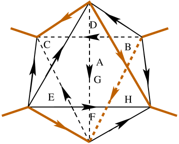
Figure 5: The braid operator ($\check{R}$-matrix) $\langle\vec{p}\ |\ \check{R}\ |\ \vec{p^{\prime}}\rangle$ is represented by the octahedron.

Figure 6: The inverse of the $\check{R}$-matrix, $\langle\vec{p}\ |\ \check{R}^{-1}\ |\ \vec{p^{\prime}}\rangle$, is represented by the same octahedron with the $\check{R}$ operator, though the content is different.

The braiding property can be seen from the realization of the $R$-operators as in Figs. 5–6. When we suppose that the gray bold lines in those figures denote the link $L$ and we look down each octahedron from the top, we find that the braiding is indeed realized as follows;

$$\langle\vec{p}\ |\ \check{R}\ |\ \vec{p^{\prime}}\rangle =\quad\lx@xy@svg{\hbox{\raise 0.0pt\hbox{\kern 11.23544pt\hbox{\ignorespaces\ignorespaces\ignorespaces\ignorespaces\ignorespaces\ignorespaces\ignorespaces\ignorespaces\ignorespaces\ignorespaces\ignorespaces\ignorespaces\ignorespaces\ignorespaces\ignorespaces\ignorespaces\ignorespaces\ignorespaces\ignorespaces\ignorespaces\ignorespaces\ignorespaces\ignorespaces\ignorespaces\ignorespaces\ignorespaces\ignorespaces\ignorespaces\ignorespaces\ignorespaces\ignorespaces{}{}{}{{}}{}\ignorespaces\ignorespaces\hbox{\hbox{\kern 0.0pt\raise 0.0pt\hbox{{}{}{}{{}{}{}}{}}}}\ignorespaces{}\ignorespaces{}{}{}{{}{}}{\hbox{\kern 21.5pt\raise 0.0pt\hbox{\hbox{\kern 0.0pt\raise 0.0pt\hbox{$\scriptstyle{\hbox to5.0pt{\hfill\vrule height=2.5pt,depth=2.5pt,width=0.0pt}}$}}}}}\ignorespaces\ignorespaces\hbox{\hbox{\kern 0.0pt\raise 0.0pt\hbox{{}{}{}{{}{}{}{{{}}{{}}{{}}{{}}{{}}{{}}{{}}{{}}{{}}{{}}{{}}{{}}{{}}{{}}{{}}{{}}{}{{}}{{}}{{}}{{}}{{}}{{}}{{}}{{}}{{}}{{}}{{}}{{}}{{}}{{}}{{}}{{}}{{}}{{}}{{}}{{}}{{}}{{}}{{}}{{}}{{}}{{}}{}}}{{}{}{}\lx@xy@spline@}{}}}}\ignorespaces{}\ignorespaces{}{}{}{{}}{}\ignorespaces\ignorespaces\hbox{\hbox{\kern 0.0pt\raise 0.0pt\hbox{{}{{}{}{}{{{}}{{}}{}{{}}{{}}{{}}{{}}{{}}{{}}{{}}{{}}{{}}{{}}{{}}{{}}{{}}{{}}{{}}{{}}{{}}{{}}{{}}}}{}{}{{}{}{}\lx@xy@spline@}{}}}}\ignorespaces{}\ignorespaces\hbox{\hbox{\kern 0.0pt\raise 0.0pt\hbox{{}{}{}{{}{}{}}{}}}}\ignorespaces{}\ignorespaces\ignorespaces\ignorespaces\ignorespaces\ignorespaces\ignorespaces\ignorespaces\ignorespaces\ignorespaces{}{}{}{{}}{}\ignorespaces\ignorespaces\hbox{\hbox{\kern 0.0pt\raise 0.0pt\hbox{{}{}{}{{}{}{}}{}}}}\ignorespaces{}\ignorespaces{}{}{}{{}}{}\ignorespaces\ignorespaces\hbox{\hbox{\kern 0.0pt\raise 0.0pt\hbox{{}{}{}{}{{}{}{}\lx@xy@spline@}{}}}}\ignorespaces{}\ignorespaces\hbox{\hbox{\kern 0.0pt\raise 0.0pt\hbox{{}{}{}{{}{}{}}{}}}}\ignorespaces{}\ignorespaces\ignorespaces\ignorespaces{\hbox{\kern-11.23544pt\raise 19.1997pt\hbox{\hbox{\kern 3.0pt\raise-1.18056pt\hbox{$\textstyle{p_{1}}$}}}}}{\hbox{\kern-2.5958pt\raise 28.8003pt\hbox{\hbox{\kern 3.0pt\raise-1.18056pt\hbox{$\textstyle{p_{2}}$}}}}}{\hbox{\kern 36.76456pt\raise 28.8003pt\hbox{\hbox{\kern 3.0pt\raise-1.18056pt\hbox{$\textstyle{p_{3}}$}}}}}{\hbox{\kern 45.88467pt\raise 18.24023pt\hbox{\hbox{\kern 3.0pt\raise-1.18056pt\hbox{$\textstyle{p_{4}}$}}}}}{\hbox{\kern-11.23544pt\raise-19.1997pt\hbox{\hbox{\kern 3.0pt\raise-1.95833pt\hbox{$\textstyle{p_{1}^{\prime}}$}}}}}{\hbox{\kern-2.5958pt\raise-28.8003pt\hbox{\hbox{\kern 3.0pt\raise-1.95833pt\hbox{$\textstyle{p_{2}^{\prime}}$}}}}}{\hbox{\kern 36.76456pt\raise-28.8003pt\hbox{\hbox{\kern 3.0pt\raise-1.95833pt\hbox{$\textstyle{p_{3}^{\prime}}$}}}}}{\hbox{\kern 45.88467pt\raise-18.24023pt\hbox{\hbox{\kern 3.0pt\raise-1.95833pt\hbox{$\textstyle{p_{4}^{\prime}}$}}}}}{}}}}}\ignorespaces \textstyle{p_{1}} \textstyle{p_{2}} \textstyle{p_{3}} \textstyle{p_{4}} \textstyle{p_{1}^{\prime}} \textstyle{p_{2}^{\prime}} \textstyle{p_{3}^{\prime}} \textstyle{p_{4}^{\prime}} \textstyle{p_{1}} \textstyle{p_{2}} \textstyle{p_{3}} \textstyle{p_{4}} \textstyle{p_{1}^{\prime}} \textstyle{p_{2}^{\prime}} \textstyle{p_{3}^{\prime}} \textstyle{p_{4}^{\prime}}$$ (5.2a)

$$\langle\vec{p}\ |\ \check{R}^{-1}\ |\ \vec{p^{\prime}}\rangle =\quad\lx@xy@svg{\hbox{\raise 0.0pt\hbox{\kern 11.23544pt\hbox{\ignorespaces\ignorespaces\ignorespaces\ignorespaces\ignorespaces\ignorespaces\ignorespaces\ignorespaces\ignorespaces\ignorespaces\ignorespaces\ignorespaces\ignorespaces\ignorespaces\ignorespaces\ignorespaces\ignorespaces\ignorespaces\ignorespaces\ignorespaces\ignorespaces\ignorespaces\ignorespaces\ignorespaces\ignorespaces\ignorespaces\ignorespaces\ignorespaces\ignorespaces\ignorespaces\ignorespaces{}{}{}{{}}{}\ignorespaces\ignorespaces\hbox{\hbox{\kern 0.0pt\raise 0.0pt\hbox{{}{}{}{{}{}{}}{}}}}\ignorespaces{}\ignorespaces{}{}{}{{}}{}\ignorespaces\ignorespaces\hbox{\hbox{\kern 0.0pt\raise 0.0pt\hbox{{}{}{}{}{{}{}{}\lx@xy@spline@}{}}}}\ignorespaces{}\ignorespaces\hbox{\hbox{\kern 0.0pt\raise 0.0pt\hbox{{}{}{}{{}{}{}}{}}}}\ignorespaces{}\ignorespaces\ignorespaces\ignorespaces\ignorespaces\ignorespaces\ignorespaces\ignorespaces\ignorespaces\ignorespaces{}{}{}{{}}{}\ignorespaces\ignorespaces\hbox{\hbox{\kern 0.0pt\raise 0.0pt\hbox{{}{}{}{{}{}{}}{}}}}\ignorespaces{}\ignorespaces{}{}{}{{}{}}{\hbox{\kern 21.5pt\raise 0.0pt\hbox{\hbox{\kern 0.0pt\raise 0.0pt\hbox{$\scriptstyle{\hbox to5.0pt{\hfill\vrule height=2.5pt,depth=2.5pt,width=0.0pt}}$}}}}}\ignorespaces\ignorespaces\hbox{\hbox{\kern 0.0pt\raise 0.0pt\hbox{{}{}{}{{}{}{}{{{}}{{}}{{}}{{}}{{}}{{}}{{}}{{}}{{}}{{}}{{}}{{}}{{}}{{}}{{}}{{}}{}{{}}{{}}{{}}{{}}{{}}{{}}{{}}{{}}{{}}{{}}{{}}{{}}{{}}{{}}{{}}{{}}{{}}{{}}{{}}{{}}{{}}{{}}{{}}{{}}{{}}{{}}{}}}{{}{}{}\lx@xy@spline@}{}}}}\ignorespaces{}\ignorespaces{}{}{}{{}}{}\ignorespaces\ignorespaces\hbox{\hbox{\kern 0.0pt\raise 0.0pt\hbox{{}{{}{}{}{{{}}{{}}{}{{}}{{}}{{}}{{}}{{}}{{}}{{}}{{}}{{}}{{}}{{}}{{}}{{}}{{}}{{}}{{}}{{}}{{}}{{}}}}{}{}{{}{}{}\lx@xy@spline@}{}}}}\ignorespaces{}\ignorespaces\hbox{\hbox{\kern 0.0pt\raise 0.0pt\hbox{{}{}{}{{}{}{}}{}}}}\ignorespaces{}\ignorespaces\ignorespaces\ignorespaces{\hbox{\kern-11.23544pt\raise 19.1997pt\hbox{\hbox{\kern 3.0pt\raise-1.18056pt\hbox{$\textstyle{p_{1}}$}}}}}{\hbox{\kern-2.5958pt\raise 28.8003pt\hbox{\hbox{\kern 3.0pt\raise-1.18056pt\hbox{$\textstyle{p_{2}}$}}}}}{\hbox{\kern 36.76456pt\raise 28.8003pt\hbox{\hbox{\kern 3.0pt\raise-1.18056pt\hbox{$\textstyle{p_{3}}$}}}}}{\hbox{\kern 45.88467pt\raise 18.24023pt\hbox{\hbox{\kern 3.0pt\raise-1.18056pt\hbox{$\textstyle{p_{4}}$}}}}}{\hbox{\kern-11.23544pt\raise-19.1997pt\hbox{\hbox{\kern 3.0pt\raise-1.95833pt\hbox{$\textstyle{p_{1}^{\prime}}$}}}}}{\hbox{\kern-2.5958pt\raise-28.8003pt\hbox{\hbox{\kern 3.0pt\raise-1.95833pt\hbox{$\textstyle{p_{2}^{\prime}}$}}}}}{\hbox{\kern 36.76456pt\raise-28.8003pt\hbox{\hbox{\kern 3.0pt\raise-1.95833pt\hbox{$\textstyle{p_{3}^{\prime}}$}}}}}{\hbox{\kern 45.88467pt\raise-18.24023pt\hbox{\hbox{\kern 3.0pt\raise-1.95833pt\hbox{$\textstyle{p_{4}^{\prime}}$}}}}}{}}}}}\ignorespaces \textstyle{p_{1}} \textstyle{p_{2}} \textstyle{p_{3}} \textstyle{p_{4}} \textstyle{p_{1}^{\prime}} \textstyle{p_{2}^{\prime}} \textstyle{p_{3}^{\prime}} \textstyle{p_{4}^{\prime}} \textstyle{p_{1}} \textstyle{p_{2}} \textstyle{p_{3}} \textstyle{p_{4}} \textstyle{p_{1}^{\prime}} \textstyle{p_{2}^{\prime}} \textstyle{p_{3}^{\prime}} \textstyle{p_{4}^{\prime}}$$ (5.2b)

We should stress that every 0-simplex of the octahedron is on the link $L$, and that the octahedron is in the complement of the link $L$.

We shall check the hyperbolicity consistency condition in constructing the $R$-operator from the ideal tetrahedra in a case of $\gamma\to 0$. Substituting the asymptotic form (4.1) into eq. (5.1), we get

$$\langle\vec{p}\ |\ \check{R}_{12,34}\ |\ \vec{p^{\prime}}\rangle\sim\delta(p_{1}-p_{2}+p_{3}-p_{1}^{\prime})\,\delta(p_{2}^{\prime}-p_{3}^{\prime}+p_{4}^{\prime}-p_{4})\\ \times\iint\mathrm{d}z\ \mathrm{d}w\ \exp\frac{1}{2\,\mathrm{i}\,\gamma}\biggl{(}-\mathrm{Li}_{2}(\mathrm{e}^{w-p_{2}})+\mathrm{Li}_{2}(\mathrm{e}^{w-p_{4}^{\prime}})-\mathrm{Li}_{2}(\mathrm{e}^{z-p_{3}^{\prime}})+\mathrm{Li}_{2}(\mathrm{e}^{z-p_{1}})\\ +(-p_{1}+p_{1}^{\prime})\,(-w+p_{2}+z-p_{1})+(p_{4}-p_{4}^{\prime})\,(w-p_{4}^{\prime}-z+p_{3}^{\prime})\biggr{)}.$$ (5.3)

Here we have used trivial constraints;

$$x =-p_{1}+p_{1}^{\prime}, y =p_{4}-p_{4}^{\prime}.$$ (5.4)

Above integral is evaluated by the saddle point, in which we have constraints

$$\frac{1-\mathrm{e}^{w-p_{2}}}{1-\mathrm{e}^{w-p_{4}^{\prime}}}\,\mathrm{e}^{p_{1}-p_{1}^{\prime}+p_{4}-p_{4}^{\prime}}=1, \frac{1-\mathrm{e}^{z-p_{3}^{\prime}}}{1-\mathrm{e}^{z-p_{1}}}\,\mathrm{e}^{-p_{1}+p_{1}^{\prime}-p_{4}+p_{4}^{\prime}}=1.$$

This set of equations solves

$$\mathrm{e}^{w} =\frac{1-\mathrm{e}^{p_{1}-p_{1}^{\prime}+p_{4}-p_{4}^{\prime}}}{\mathrm{e}^{-p_{4}^{\prime}}-\mathrm{e}^{p_{1}-p_{1}^{\prime}+p_{4}-p_{4}^{\prime}-p_{2}}}, \mathrm{e}^{z} =\frac{1-\mathrm{e}^{p_{1}-p_{1}^{\prime}+p_{4}-p_{4}^{\prime}}}{\mathrm{e}^{-p_{3}^{\prime}}-\mathrm{e}^{p_{1}-p_{1}^{\prime}+p_{4}-p_{4}^{\prime}-p_{1}}},$$ (5.5)

and we easily find a constraint,

$$\frac{1-\mathrm{e}^{w-p_{2}}}{1-\mathrm{e}^{w-p_{4}^{\prime}}}\cdot\frac{1-\mathrm{e}^{z-p_{3}^{\prime}}}{1-\mathrm{e}^{z-p_{1}}}=1,$$ (5.6)

which coincides with the hyperbolicity condition around vertical axis (crossing point in eq (5.2)).

Due to the symmetry of the $R$-operator (2.29), we can conclude that for each crossing in a link $L$ we can attach the oriented octahedron, which has a following projection;

(5.7)

Here $x$ and $y$ are auxiliary momenta given by eq. (5.4), and $w$ and $z$ are fixed by eq. (5.5). We further have

$$p_{3} =-p_{1}+p_{2}+p_{1}^{\prime}, p_{2}^{\prime} =p_{4}+p_{3}^{\prime}-p_{4}^{\prime}.$$ (5.8)

and the dihedral angles $a_{i}$ satisfying $a_{1}\,a_{2}\,a_{3}\,a_{4}=1$ are given by

$$a_{1} =(1-\mathrm{e}^{z-p_{1}})^{-1}=\frac{\mathrm{e}^{p_{1}-p_{1}^{\prime}+p_{4}-p_{4}^{\prime}}-\mathrm{e}^{p_{1}-p_{3}^{\prime}}}{1-\mathrm{e}^{p_{1}-p_{3}^{\prime}}},$$

$$a_{2} =1-\mathrm{e}^{z-p_{3}^{\prime}}=\frac{1-\mathrm{e}^{p_{1}-p_{3}^{\prime}}}{1-\mathrm{e}^{-p_{1}+p_{1}^{\prime}-p_{4}+p_{4}^{\prime}}\mathrm{e}^{p_{1}-p_{3}^{\prime}}},$$

$$a_{3} =(1-\mathrm{e}^{w-p_{4}^{\prime}})^{-1}=\frac{1-\mathrm{e}^{-p_{1}+p_{1}^{\prime}-p_{4}+p_{4}^{\prime}}\mathrm{e}^{p_{2}-p_{4}^{\prime}}}{1-\mathrm{e}^{p_{2}-p_{4}^{\prime}}},$$

$$a_{4} =1-\mathrm{e}^{w-p_{2}}=\frac{1-\mathrm{e}^{p_{2}-p_{4}^{\prime}}}{\mathrm{e}^{p_{1}-p_{1}^{\prime}+p_{4}-p_{4}^{\prime}}-\mathrm{e}^{p_{2}-p_{4}^{\prime}}}.$$

To close this section, we give an explicit form of an asymptotic form of the $\check{R}$-operators. As the integral (2.28) has an asymptotic form,

$$H(a,b,c,d)\\ \sim\exp\frac{1}{2\,\mathrm{i}\,\gamma}\biggl{(}\mathrm{Li}_{2}(\mathrm{e}^{a-b})+\mathrm{Li}_{2}(\mathrm{e}^{d-a})-\mathrm{Li}_{2}(\mathrm{e}^{c-b})-\mathrm{Li}_{2}(\mathrm{e}^{d-c})+c\,(-a+b-c+d)\biggr{)},$$ (5.9)

the $\check{R}^{\pm 1}$ operators in a limit $\gamma\to 0$ are respectively given by

$$\langle\vec{p}\ |\ \check{R}_{12,34}\ |\ \vec{p^{\prime}}\rangle\sim\delta(p_{1}+p_{3}-p_{2}-p_{1}^{\prime})\cdot\delta(p_{2}^{\prime}-p_{3}^{\prime}+p_{4}^{\prime}-p_{4})\\ \times\exp\frac{1}{2\,\mathrm{i}\,\gamma}\biggl{(}\mathrm{Li}_{2}(\mathrm{e}^{p_{4}-p_{3}})+\mathrm{Li}_{2}(\mathrm{e}^{p_{3}^{\prime}-p_{1}})-\mathrm{Li}_{2}(\mathrm{e}^{p_{4}^{\prime}-p_{2}})-\mathrm{Li}_{2}(\mathrm{e}^{p_{2}^{\prime}-p_{1}^{\prime}})\\ +(p_{1}^{\prime}-p_{1})\,(-p_{4}+p_{3}-p_{1}^{\prime}+p_{2}^{\prime})\biggr{)},$$ (5.10a)

$$\langle\vec{p}\ |\ (\check{R}_{12,34})^{-1}\ |\ \vec{p^{\prime}}\rangle\sim\delta(p_{4}^{\prime}-p_{2}+p_{3}-p_{4})\,\delta(p_{1}-p_{1}^{\prime}-p_{3}^{\prime}+p_{2}^{\prime})\\ \times\exp\frac{1}{2\,\mathrm{i}\,\gamma}\biggl{(}\mathrm{Li}_{2}(\mathrm{e}^{p_{2}-p_{1}})+\mathrm{Li}_{2}(\mathrm{e}^{p_{4}-p_{2}^{\prime}})-\mathrm{Li}_{2}(\mathrm{e}^{p_{3}-p_{1}^{\prime}})-\mathrm{Li}_{2}(\mathrm{e}^{p_{4}^{\prime}-p_{3}^{\prime}})\\ +(p_{1}-p_{1}^{\prime})\,(p_{1}-p_{2}-p_{3}^{\prime}+p_{4}^{\prime})\biggr{)}.$$ (5.10b)

In constructing the knot invariant $\tau_{1}(K)$, we need another operator $\mu$ (3.5). The matrix element of the $\mu$-operator can be computed simply, and in the classical limit $\gamma\to 0$ reduces to

$$\langle p_{1},p_{2}\ |\ \mu\ |\ p_{1}^{\prime},p_{2}^{\prime}\rangle\sim\delta(p_{1}-p_{1}^{\prime})\,\delta(p_{2}-p_{2}^{\prime})\cdot\exp\frac{\pi}{\gamma}\bigl{(}p_{1}-p_{2}\bigr{)}.$$ (5.11)

Thus the saddle point condition coming from the $\mu$-operator is always $2\,\pi\,\mathrm{i}$, and we can ignore a contribution from the $\mu$-operator to the saddle point condition.

In the rest of this section, we study how to glue these octahedra in the invariant $\tau_{1}(K)$. We show that for every gluing there exists a correspondence between the saddle point equations and the hyperbolicity consistency conditions around edge.

5.2 Hyperbolicity Condition for Surface

We first consider a surface $D_{a}$, which is surrounded by alternating crossings as in Fig. 7. We assign octahedron for each crossing following eq. (5.7), and introduce variables as shown there.

Figure 7: A segment of link $L$ which is surrounded by alternating crossings is depicted. We number each vertex as ①, ②, $\ldots$.

A contribution to the invariant $\tau_{1}(L)$ from above segment of link $L$ is thus given by

$$\iiint\mathrm{d}p_{1}\cdots\mathrm{d}p_{n}\ \prod_{i=0}^{n-1}\langle p_{i+1},x_{i+1}\ |\ S^{-1}\ |\ y_{i},p_{i}\rangle,$$ (5.12)

where we use $y_{0}=y_{n}$ and $p_{0}=p_{n}$. By substituting an asymptotic form (4.1), we get $p_{i+1}=p_{1}+\sum_{j=1}^{i}y_{j}$ for $i>0$, and the integral reduces to

$$\delta(y_{1}+\dots+y_{n})\cdot\int\mathrm{d}p_{1}\ \exp\frac{1}{2\,\mathrm{i}\,\gamma}\biggl{(}\sum_{i=0}^{n-1}\Bigl{(}\frac{\pi^{2}}{6}-\mathrm{Li}_{2}(\mathrm{e}^{x_{i+1}-p_{i}})-x_{i+1}\,y_{i}\Bigr{)}+\sum_{1\leq i<j\leq n}y_{i}\,y_{j}\biggr{)}.$$

We evaluate this integral at the saddle point, whose condition is

$$\prod_{i=0}^{n-1}\bigl{(}1-\mathrm{e}^{x_{i+1}-p_{i}}\bigr{)}=1.$$ (5.13)

This equation coincides with the hyperbolicity condition for gluing $n$ tetrahedra in surface $D_{a}$ along an axis parallel to axes $\otimes$ in Fig. 7 (see also Fig. 14 and Fig. 16 for $n=3$ and $n=2$ cases).

We can see that the same correspondence occurs for non-alternating case. We suppose a surface $D_{a}$ is surrounded like Fig. 7 whereas each vertex $i$ is either over-crossing or under-crossing , which we denote $i\in\mathcal{O}$ and $i\in\mathcal{U}$ respectively. In this case a contribution to the invariant is given by

$$\iiint\mathrm{d}p_{1}\cdots\mathrm{d}p_{n}\ \prod_{i\in\mathcal{O}}\langle p_{i+1},x_{i+1}\ |\ S^{-1}\ |\ y_{i},p_{i}\rangle\cdot\prod_{i\in\mathcal{U}}\langle x_{i+1},p_{i+1}\ |\ S\ |\ p_{i},y_{i}\rangle.$$ (5.14)

By substituting an expression (4.1) we obtain

$$p_{k+1} =p_{1}+\sum_{\begin{subarray}{c}1\leq i\leq k\\ i\in\mathcal{O}\end{subarray}}y_{i}-\sum_{\begin{subarray}{c}1\leq i\leq k\\ i\in\mathcal{U}\end{subarray}}x_{i+1}, \sum_{i\in\mathcal{O}}y_{i}=\sum_{i\in\mathcal{U}}x_{i+1},$$

and the integral becomes

$$\delta(\sum_{i\in\mathcal{O}}y_{i}-\sum_{i\in\mathcal{U}}x_{i+1})\int\mathrm{d}p_{1}\ \exp\frac{1}{2\,\mathrm{i}\,\gamma}\biggl{(}\sum_{i\in\mathcal{O}}\Bigl{(}\frac{\pi^{2}}{6}-\mathrm{Li}_{2}(\mathrm{e}^{x_{i+1}-p_{i}})-x_{i+1}\,y_{i}\Bigr{)}\\ +\sum_{i\in\mathcal{U}}\Bigl{(}-\frac{\pi^{2}}{6}+\mathrm{Li}_{2}(\mathrm{e}^{y_{i}-p_{i+1}})+x_{i+1}\,y_{i}\Bigr{)}+\sum_{\begin{subarray}{c}i,j\in\mathcal{O}\\ i<j\end{subarray}}y_{i}\,y_{j}-\sum_{\begin{subarray}{c}i\in\mathcal{U}\\ j\in\mathcal{O}\end{subarray}}x_{i+1}\,y_{j}+\sum_{\begin{subarray}{c}i,j\in\mathcal{U}\\ i\leq j\end{subarray}}x_{i+1}\,x_{j+1}\biggr{)}.$$

The saddle point equation is given as

$$\prod_{i\in\mathcal{O}}\Bigl{(}1-\mathrm{e}^{x_{i+1}-p_{i}}\Bigr{)}\cdot\prod_{i\in\mathcal{U}}\Bigl{(}1-\mathrm{e}^{y_{i}-p_{i+1}}\Bigr{)}^{-1}=1,$$ (5.15)

which coincides with the hyperbolicity equation around an axis in $D_{a}$ parallel to axes $\otimes$.

5.3 Gluing Around Ridgeline of Octahedron

We shall check a correspondence between the hyperbolic condition and the saddle point equation for ridgelines of octahedron. We consider a case such as Fig. 8. Therein $n-1$ over-crossings are sandwiched by two under-crossings .

Figure 8: We parameterize a segment of link $L$.

A contribution from this segment is given by

$$\iiint\prod_{i=1}^{n}\mathrm{d}p_{i,1}\ \mathrm{d}p_{i,2}\cdot\mathrm{d}x_{1}\ \mathrm{d}x_{4}\ \langle x_{1},p_{1,1}\ |\ S\ |\ p_{1,3},x_{2}\rangle\,\langle p_{1,4},x_{3}\ |\ S^{-1}\ |\ x_{1},p_{1,2}\rangle\\ \times\prod_{j=1}^{n-1}\langle p_{j,5},p_{j+1,3},p_{j+1,1},p_{j+1,2}\ |\ \check{R}\ |\ p_{j,1},p_{j,2},p_{j,6},p_{j+1,4}\rangle\\ \times\langle p_{n,5},x_{5}\ |\ S^{-1}\ |\ x_{4},p_{n,1}\rangle\,\langle x_{4},p_{n,2}\ |\ S\ |\ p_{n,6},x_{6}\rangle.$$ (5.16)

We substitute eqs. (4.1) and (5.10) into above equation. We get

$$p_{j,1} =p_{j+1,1}-p_{j+1,3}+p_{j,5}, p_{j,2} =p_{j+1,2}-p_{j+1,4}+p_{j,6},$$

$$p_{n,1} =-x_{4}+p_{n,5}, p_{n,2} =-x_{4}+p_{n,6},$$

$$x_{1} =x_{4}+\sum_{j=1}^{n}(p_{j,3}-p_{j,5}),$$

and the integral reduces to that of $x_{4}$-integration, whose saddle point equation is given by

$$\frac{(1-\mathrm{e}^{x_{3}-p_{1,2}})\,(1-\mathrm{e}^{x_{5}-p_{n,1}})}{(1-\mathrm{e}^{x_{2}-p_{1,1}})\,(1-\mathrm{e}^{x_{6}-p_{n,2}})}\cdot\mathrm{e}^{+x_{2}-x_{3}-x_{5}+x_{6}}=1.$$

One sees that this equation coincides with the hyperbolicity equation around a ridgeline of the octahedron (bold lines in Fig 9);

$$\frac{1-\mathrm{e}^{p_{1,1}-x_{2}}}{1-\mathrm{e}^{p_{1,2}-x_{3}}}\cdot\prod_{j=1}^{n-1}\mathrm{e}^{-p_{j,5}+p_{j,6}+p_{j+1,3}-p_{j+1,4}}\cdot\frac{1-\mathrm{e}^{p_{n,2}-x_{6}}}{1-\mathrm{e}^{p_{n,1}-x_{5}}}=1.$$ (5.17)

Figure 9: The 3-dimensional picture of Fig. 8 is given. Eq. (5.17) coincides with the hyperbolicity condition around ridgelines (bold line) of the octahedra.

In the same manner, we can see a correspondence between the saddle point equation and the hyperbolicity condition in a case that $n-1$ under-crossings are sandwiched by two over-crossings . (Fig. 10).

Figure 10: A segment of link $L$.

In this case a contribution to the invariant is given by the integral,

$$\iiint\prod_{j=1}^{n}\mathrm{d}p_{j,1}\ \mathrm{d}p_{j,2}\cdot\mathrm{d}x_{1}\ \mathrm{d}x_{4}\ \langle p_{1,1},x_{1}\ |\ S^{-1}\ |\ x_{2},p_{1,3}\rangle\,\langle x_{3},p_{1,4}\ |\ S\ |\ p_{1,2},x_{1}\rangle\\ \times\prod_{j=1}^{n-1}\langle p_{j,2},p_{j,1},p_{j,5},p_{j+1,3}\ |\ \check{R}\ |\ p_{j,6},p_{j+1,4},p_{j+1,2},p_{j+1,1}\rangle\\ \times\langle x_{5},p_{n,5}\ |\ S\ |\ p_{n,1},x_{4}\rangle\,\langle p_{n,2},x_{4}\ |\ S^{-1}\ |\ x_{6},p_{n,6}\rangle.$$ (5.18)

By substituting eqs. (4.1) and (5.10), we obtain

$$p_{j,2} =p_{j,1}-p_{j,5}+p_{j,6}, p_{1,1} =p_{1,3}+x_{2},$$

$$p_{n,1} =x_{5}+p_{n,5}, p_{n,2} =x_{6}+p_{n,6},$$

and the integral reduces to an integration over $x_{1}$, $x_{4}$, and $p_{j,1}$ for $j=2,3,\dots,n-1$. The saddle point equations for $x_{1}$ and $x_{4}$ are respectively written as

$$\frac{1-\mathrm{e}^{x_{1}-p_{1,3}}}{1-\mathrm{e}^{x_{1}-p_{1,4}}}\cdot\mathrm{e}^{-x_{2}+x_{3}} =1, \frac{1-\mathrm{e}^{x_{4}-p_{n,6}}}{1-\mathrm{e}^{x_{4}-p_{n,5}}}\cdot\mathrm{e}^{-x_{6}+x_{5}} =1.$$

These two equations give

$$\frac{1-\mathrm{e}^{p_{1,4}-x_{1}}}{1-\mathrm{e}^{p_{1,3}-x_{1}}}\cdot\prod_{j=1}^{n-1}\mathrm{e}^{-p_{j,2}+p_{j+1,2}-p_{j+1,1}+p_{j,1}}\cdot\frac{1-\mathrm{e}^{p_{n,5}-x_{4}}}{1-\mathrm{e}^{p_{n,6}-x_{4}}}=1,$$ (5.19)

which denotes the hyperbolicity equation around ridgelines of the octahedron (Fig. 11).

Figure 11: Depicted are polyhedra which come from Fig. 10. The hyperbolicity condition around bold edges is given in eq. (5.19).

As a result, we have seen that the 3-dimensional hyperbolic structure naturally appears in the invariant $\tilde{\tau}_{1}(K)$, i.e., a classical limit of the knot invariant $\tau_{1}(K)$ which is defined by the integral form based on the quantum dilogarithm function. The saddle point equation exactly coincides with the hyperbolicity consistency condition in gluing the octahedra which is assigned to each crossing. To be precise, in order to see that a finite collection of ideal tetrahedra results in a 3-manifold, we need to prove the completeness condition by showing that the developing map near the ideal vertex yields Euclidean structure. We have checked this condition for several knots, but we do not have proof at this moment. There is still another problem to be solved. Generally a set of the saddle point equations (hyperbolicity consistency conditions) has several algebraic solutions, and we are not sure which solutions among them we should choose as dominant in a definition of the invariant $\tilde{\tau}_{1}(K)$. When we assume that geometrically preferable solutions $z_{i}$ of the saddle point conditions are dominant in the classical limit, we may conclude that

$$\tilde{\tau}_{1}(K) =\sum_{\text{ideal tetrahedra}:i}L(1-z_{i}),$$ (5.20)

as each tetrahedron has a function $V(x,y)$ which reduces to the Rogers dilogarithm function at the critical point (4.3).

6 Example: Figure-Eight Knot

We shall demonstrate how to decompose the knot complement into tetrahedra in a case of the figure-eight knot. The figure-eight knot is given as $\sigma_{1}\,\sigma_{2}^{~{}-1}\,\sigma_{1}\,\sigma_{2}^{~{}-1}$ in the braid group, and is depicted as Fig. 12. To each crossing in the figure-eight knot, we assign the octahedron (Fig. 5 or eq. (5.7)), and give the numbering to each crossing as in Fig. 13. We have also named each surface as $D_{i}$. We call the surface inside the octahedron as $S^{a}_{i,j}$; a surface is in the octahedron of the $a$-th crossing, and is a boundary between $D_{i}$ and $D_{j}$.

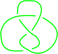
Figure 12: The figure-eight knot $4_{1}$.

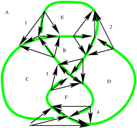
Figure 13: We attach octahedra for each crossing of the figure-eight knot.

In a surface $D_{1}$ there are 3 tetrahedra. These three tetrahedra are glued to each other as shown in Fig. 14. Due to the pentagon relation we obtain 2 adjacent tetrahedra, whose common surface (gray surface) is named $P_{1}$.

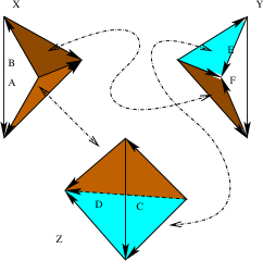
$\Longleftrightarrow$   

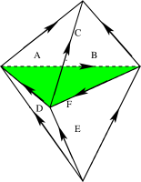
Figure 14: Gluing 3 tetrahedra in surface $D_{1}$ results in 2 tetrahedra by the 2-3 Pachner move. The gray surface in the 2 adjacent tetrahedra is called $P_{1}$.

Three tetrahedra in a surface $D_{0}$ also gives same adjacent tetrahedra with that in Fig. 14. By the same method of gluing 3 tetrahedra in surfaces $D_{2}$ and $D_{3}$, we obtain adjacent tetrahedra as shown in Fig. 15.

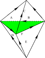
(a) (b)  (c) 

Figure 15: Gluing 3 tetrahedra in surfaces (a) $D_{0}$, (b) $D_{2}$, and (c) $D_{3}$ gives the 2 adjacent tetrahedra. We call each gray surface respectively $P_{0}$, $P_{2}$, and $P_{3}$.

In a surface $D_{4}$, we have 2 tetrahedra, which are glued to each other and result in a suspension as shown in Fig. 16. We also get a suspension from a surface $D_{5}$ as is shown in Fig. 17.

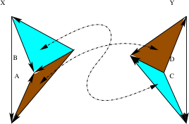
$\Longleftrightarrow$   

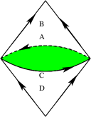
Figure 16: Gluing 2 tetrahedra in a surface $D_{4}$ gives a suspension.

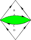
Figure 17: Gluing 2 tetrahedra in a surface $D_{5}$.

We next glue these polyhedra, 4 2-adjacent-tetrahedra (Fig. 14 and Fig. 15) and 2 suspensions (Fig. 16 and Fig. 17). We first cut those polyhedra in the plane which was painted gray in figures, and separate them into “upper” and “lower” polyhedra (tetrahedra or cones). In this procedure, we should remember which vertices in the gray faces were glued to each other. We then glue these polygons to each other which have same surfaces $S^{a}_{i,j}$, and we finally obtain 2 tetrahedra (Fig. 18) which come from upper and lower polyhedra. Faces in these tetrahedra present gray faces in Figs. 14–15 which separates upper and lower polyhedra. It is a well known result by Thurston [5] that the complement of the figure-eight knot is decomposed into these 2 tetrahedra. Note that, in order to have upper and lower polyhedra, we have used the so-called 1-4 Pachner move which shows that neighborhood of vertex inside the tetrahedron constitute sphere as was pointed out in Ref. 8.

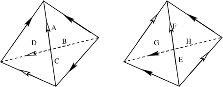
Figure 18: Complement of the figure-eight knot.

The partition function of the complement of the figure-eight knot is then computed from Fig. (18) as

$${\tau}_{1}({4_{1}}) =\int\mathrm{d}\vec{p}\ \langle p_{1}=0,p_{2}\ |\ S\ |\ p_{3},p_{4}\rangle\,\langle p_{4},p_{3}\ |\ S^{-1}\ |\ p_{2},p_{1}=0\rangle$$

$$\sim\int\mathrm{d}p\ \exp\frac{1}{2\,\mathrm{i}\,\gamma}\,\Bigl{(}\mathrm{Li}_{2}(\mathrm{e}^{-p})-\mathrm{Li}_{2}(\mathrm{e}^{p})\Bigr{)}.$$ (6.1)

Here we have introduced a restriction $p_{1}=0$ which comes from a computation of the knot invariant for a ($1,1$)-tangle. The integral in the partition function can be evaluated at the saddle point,

$$(1-\mathrm{e}^{p})\,(1-\mathrm{e}^{-p})=1,$$

which, with a root of $\omega^{2}-\omega+1=0$, gives

$$\tilde{\tau}_{1}(4_{1})=\lim_{\gamma\to 0}\left(2\,\mathrm{i}\,\gamma\log{\tau}_{1}(4_{1})\right)=2.02988\,\mathrm{i}.$$ (6.2)

The imaginary part is nothing but the hyperbolic volume of the complement of the figure-eight knot.

7 Concluding Remarks

We have studied the knot invariant by use of the infinite dimensional representation of the quantum dilogarithm function. This invariant can be seen by construction as the non-compact analogue of the colored Jones polynomial. We have found that, by assigning the oriented tetrahedra to the $S$-operator which solves the five-term relation, the braid operators can be depicted as the octahedron as was shown in Ref. 10. With this realization, we have obtained a general scheme to triangulate the knot complements. This method can be applicable for arbitrary knots and links, whereas methods in Refs. 24, 25 seem to work only for the alternating knots. We have further revealed that the hyperbolic structure appears in the classical limit of our invariant, and that the hyperbolicity consistency conditions in gluing ideal tetrahedra coincide exactly with the saddle point equations of integrals of knot invariant. Based on the result that an imaginary part of the $S$-operator (2.20) reduces to the Bloch–Wigner function at the critical point (4.3), and that we can identify the $S$-operator as the oriented ideal tetrahedron whose dihedral angles are fixed, we can conclude that the imaginary part of the invariant $\tilde{\tau}_{1}(K)$ will give the hyperbolic volume

$$\text{Im}\,\tilde{\tau}_{1}(K) =\sum_{\text{ideal tetrahedra}:i}D(z_{i}),$$

though we are not sure which solutions of a set of the hyperbolicity conditions are dominant in the classical limit.

From the physical view points, the Jones polynomial is closely related with the topological gauge field theory in 3-dimension [26]. Therein the Chern–Simons path integral becomes the invariant of the 3-manifold, and in Ref. 27 Dijkgraaf and Witten gave a combinatorial definition for the Chern–Simons invariants $\mathrm{CS}(M)$ of the manifold $M$ by use of 3-cocycles of the group cohomology [27]. What is interesting here is that, with the hyperbolic volume $\mathrm{Vol}(M)$, the function $\mathrm{Vol}(M)+\mathrm{i}\,\mathrm{CS}(M)$ is analytic and depends on element $\beta(M)$ of the (orientation sensitive) scissors congruence group [28, 29]. With a suitable setting of branches of the log function, the element of the scissors congruence group for non-compact manifold $M$ is known to be given by [30]

$$\beta(M)=\sum_{\text{ideal triangulation $z_{i}$}}L(1-z_{i}),$$ (7.1)

where $L(z)$ is the Rogers dilogarithm function (2.2). As we have shown that the invariant $\tilde{\tau}_{1}(K)$ is given by eq. (5.20) based on that the $S$-operator in the classical limit gives the Rogers dilogarithm function at the critical point (4.3), it is a natural consequence that our non-compact colored Jones invariant (3.7) may give the Chern–Simons term,

$$\tilde{\tau}_{1}(K)=\lim_{\gamma\to 0}\Bigl{(}2\,\mathrm{i}\,\gamma\log\tau_{1}(K)\Bigr{)}=\mathrm{i}\,\Bigl{(}\mathrm{Vol}(K)+\mathrm{i}\,\mathrm{CS}(K)\Bigr{)}.$$ (7.2)

References

- [1] V. F. R. Jones: Bull. Amer. Math. Soc. 12, 103 (1985).
- [2] V. Turaev: Invent. Math. 92, 527 (1988).
- [3] R. M. Kashaev: Mod. Phys. Lett. A 10, 1409 (1995).
- [4] R. M. Kashaev: Lett. Math. Phys. 39, 269 (1997).
- [5] W. P. Thurston: The Geometry and Topology of Three-Manifolds, Lecture Notes in Princeton University, Princeton (1980).
- [6] J. Milnor: Bull. Amer. Math. Soc. 6, 9 (1982).
- [7] H. Murakami and J. Murakami: Acta Math., to appear (math.GT/9905075).
- [8] Y. Yokota: preprint (math.QA/0009165).
- [9] H. Murakami: preprint (math.GT/0008027).
- [10] D. Thurston: Hyperbolic volume and the Jones polynomial. Lecture notes of École d’été de Mathématiques ‘Invariants de nœuds et de variétés de dimension 3’, Institut Fourier (1999).
- [11] L. Lewin, ed.: Structural Properties of Polylogarithm, Mathematical Surveys and Monographs 37 (Amer. Math. Soc., Providence, 1991).
- [12] A. N. Kirillov: Prog. Theor. Phys. Suppl. 118, 61 (1995).
- [13] L. D. Faddeev: In Quantum Groups and Their Applications in Physics (Edited by L. Castellani and J. Wess) (IOS Press, Amsterdam, 1996) pp. 117–136.
- [14] S. N. M. Ruijsenaars: J. Math. Phys. 38, 1069 (1997).
- [15] S. L. Woronowicz: Rev. Math. Phys. 12, 873 (2000).
- [16] L. D. Faddeev and R. M. Kashaev: Mod. Phys. Lett. A 9, 427 (1994).
- [17] L. Chekhov and V. V. Fock: Theor. Math. Phys. 120, 1245 (1999).
- [18] L. D. Faddeev: preprint (math.QA/9912078).
- [19] L. D. Faddeev, R. M. Kashaev, and A. Yu. Volkov: preprint (hep-th/0006156).
- [20] B. Ponsot and J. Teschner: preprint (math.QA/0007097).
- [21] R. M. Kashaev: St. Petersburg Math. J. 8, 585 (1997).
- [22] R. M. Kashaev: In Geometry and Integrable Models (Edited by P. N. Pyatov and S. N. Solodukhn) (World Scientific, Singapore, 1996) pp. 32–51.
- [23] K. Hikami: RIMS Kôkyûroku 1172, 44 (2000).
- [24] M. Takahashi: Tsukuba J. Math. 9, 41 (1985).
- [25] C. Petronio: Geom. Dedicata 66, 27 (1997).
- [26] E. Witten: Commun. Math. Phys. 121, 351 (1989).
- [27] R. Dijkgraaf and E. Witten: Commun. Math. Phys. 129, 393 (1990).
- [28] W. Z. Neumann and D. Zagier: Topology 24, 307 (1985).
- [29] T. Yoshida: Invent. Math. 81, 473 (1985).
- [30] W. D. Neumann and J. Yang: Duke Math. J. 96, 29 (1999). 1, 72 (1995).