Many-body scattering theory of electronic systems

Abstract

This work reviews recent advances in the analytical treatment of the continuum spectrum of correlated few-body non-relativistic Coulomb systems. The exactly solvable two-body problem serves as an introduction to the non-separable three-particle system. For the latter case we discuss the existence of an approximate separability of the long and the short-range dynamics which is exposed in an appropriately chosen curvilinear coordinates. The three-body wave functions of the long-ranged part of the Hamiltonian are derived and methods are presented to account approximately for the short-ranged dynamics. Furthermore, we present a generalization of the methods employed for the derivation of the three-body wave functions to the scattering states of $N$ charged particles. To deal with thermodynamic properties of finite systems we develop and discuss a recent Green function methodology designed for the non-perturbative regime. In addition, we give a brief account on how thermodynamic properties and critical phenomena can be exposed in finite interacting systems.

1 Introduction

The theoretical treatment of many-body systems is of a fundamental importance for a variety of branches in physics. Of particular relevance to this work are highly excited systems that consist of a finite number of charged particles. Such systems are encountered in processes involving simultaneous excitations of few particles, e.g. as is the case in a multiple ionization reaction. From a theoretical point of view it is fortunate that the scattering states of two particles interacting via the Coulomb potential are known exactly, for such states can serve as a benchmark for approximate methods that are developed to deal with more complex systems. For example, the perturbative (Born) treatment of the two-particle Coulomb scattering and the comparison with the exact results gives a first hint on the problems connected with treatment of Coulomb scattering: The first order term of the Born perturbation series delivers already the correct results for the scattering cross section. Higher order terms are however divergent. This problem is mainly traced back to the infinite range of the Coulomb interaction that prohibits free motion in the asymptotic regime.

In the theoretical treatment of more than two particle systems a further fundamental difficulty arises which stems from the inherent non-separability of many-body interacting systems. This problem is of a general nature and appears basically for almost all forms of the inter-particle interactions.

This work provides an overview on recent theoretical efforts to tackle analytically the problems connected with the infinite-range tail of Coulomb potentials and the non-seprabale aspects of many-body systems. As will be shown below, generally this can be done only in an approximate way. To deal with the long-range Coulomb interaction one dismisses the use of standard many-body approaches and attempts at a direct (approximate) solution of the many-body non-relativistic Schrödinger equation. To expose the general feature of Coulomb potential scattering and to introduce the basic methods used to solve the Schrödinger equation we start with a brief review of the two-particle Rutherford scattering. The three-body Coulomb scattering problem has received recently much of attention [2, 3, 4, 5, 6, 7, 8, 9, 10, 11, 12, 13]. In this work we focus only on one aspect of this problem, namely the existence of an approximate separability that allows to derive three-body wave functions valid in certain region of the Hilbert space. For the general case of a system consisting of $N$ interacting charged particles we derive correlated scattering states that are to a first order in the distance exact at larger inter-particle separation.

The wave function approach is of a limited value when it comes to the study of thermodynamic properties and critical phenomena in finite systems. In this case detailed information on the density of states is needed. Such information is encompassed in the many-body Green function. Therefore we devote a section of this work to a general scheme for the derivation of the many-body Green operator and briefly review a possible method to extract thermodynamic information on finite systems starting from the Green function.

Unless otherwise stated we employ atomic units throughout and neglect relativistic corrections.

2 Two charged particle scattering

To introduce the general frame work and the basic notation let us consider the non-relativistic scattering states of two charged particles with charges $z_{1}$ and $z_{2}$. The Schrödinger equation describing the motion in the two-particle relative coordinate ${\bf r}$ is

$$\left[-\frac{1}{2\mu}\Delta+\frac{z_{1}z_{2}}{r}-E\right]\Psi_{\bf k}({\bf r})=0.$$ (1)

Here ${\bf k}$ is the momentum conjugate to ${\bf r}$ and $E=k^{2}/2\mu$ is the energy of the relative motion. $\mu$ is the reduced mass of the two particles. To decouple kinematics from dynamics we make the ansatz:

$$\Psi_{\bf k}({\bf r})=e^{i{\bf k}\cdot{\bf r}}\bar{\Psi}_{\bf k}({\bf r}).$$ (2)

The distortion factor $\bar{\Psi}$ in Eq.(2) is solely due to the presence of the potential. The asymptotic properties of (1) follows upon substitution of (2) in (1). Then, terms that fall off faster than the Coulomb potential can be neglected which leads to the equation

$$\left[-\frac{i}{\mu}{\bf k}\cdot{\bf\nabla}+\frac{z_{1}z_{2}}{r}\right]\bar{\Psi}_{\bf k}({\bf r})=0.$$ (3)

This equation can be solved by the ansatz $\bar{\Psi}=\exp(i\phi)$. Upon insertion in Eq.(3) this ansatz yields

$$\phi^{\pm}_{\bf k}({\bf r})=\pm\frac{z_{1}z_{2}\mu}{k}\ln a(r\mp\hat{\bf k}\cdot{\bf r}).$$ (4)

The factor $z_{1}z_{2}\mu/k$ is called the Sommerfeld parameter and characterizes the strength of the interaction. The integration constant $a$ has a dimension of a reciprocal length and the value $a=k$. The important point here is that the natural coordinate that appears in the treatment of Coulomb scattering is the so-called parabolic coordinate $\xi^{\pm}:=r\mp\hat{\bf k}\cdot{\bf r}$ where the $+$ or $-$ corresponds respectively to incoming or outgoing-wave boundary conditions.

3 The three-particle coulomb continuum states

In contrast to the two-body problem, an exact derivation of the three-body quantum states is not possible. Nonetheless, under certain (asymptotic) assumptions analytical solutions can be obtained that contain some general features of the two-body scattering, such as the characteristic asymptotic phases. As in the preceding section the center-of-mass motion of a three-body system can be factored out. The internal motion of the three charged particles with masses $m_{i}$ and charges $z_{i}\ ;i\in{1,2,3}$ can be described by one set of the three Jacobi coordinates $({\bf r}_{ij},{\bf R}_{k});\ i,j,k\in\{1,2,3\};\epsilon_{ijk}\neq 0;\ j>i$. Here ${\bf r}_{ij}$ is the relative internal separation of the pair $ij$ and ${\bf R}_{k}$ is the position of the third particle ($k$) with respect to the center of mass of the pair $ij$. The three sets of Jacobi coordinates are connected with each other via the transformation

$$\left(\begin{array}[]{c}{{\bf r}_{3}}\\ {\bf R}_{2}\end{array}\right)={\mbox{{\bf D}}_{1}}\left(\begin{array}[]{c}{{\bf r}_{23}}\\ {{\bf R}_{1}}\end{array}\right)\hskip 8.5359pt\mbox{and}\hskip 8.5359pt\left(\begin{array}[]{c}{{\bf r}_{12}}\\ {{\bf R}_{3}}\end{array}\right)={\mbox{{\bf D}}_{2}}\left(\begin{array}[]{c}{{\bf r}_{23}}\\ {{\bf R}_{1}}\end{array}\right)\$$ (13)

where

$${\mbox{{\bf D}}_{1}} = \left(\begin{array}[]{cc}\mu_{23}/m_{3}&1\\ 1-\mu_{13}\cdot\mu_{23}/m_{3}^{2}&-\mu_{13}/m_{3}\end{array}\right)$$ (16)

$${\mbox{{\bf D}}_{2}} = \left(\begin{array}[]{cc}-\mu_{23}/m_{2}&1\\ -1+\mu_{12}\cdot\mu_{23}/m_{2}^{2}&-\mu_{12}/m_{2}\end{array}\right)\$$ (19)

The reduced masses are defined as $\mu_{ij}=m_{i}m_{j}/(m_{i}+m_{j})\ ;\ i,j\in\{1,2,3\};\ j>i$. Accordingly, the momenta conjugate to (${\bf r}_{ij},{\bf R}_{k}$) are defined as $({\bf k}_{ij},{\bf K}_{k})$. These momenta are related to each other by

$$\left(\begin{array}[]{c}{{\bf k}_{23}}\\ {\bf K}_{1}\end{array}\right) = {\mbox{{\bf D}}_{2}}^{t}\left(\begin{array}[]{c}{{\bf k}_{12}}\\ {{\bf K}_{3}}\end{array}\right)={\mbox{{\bf D}}_{1}}^{t}\left(\begin{array}[]{c}{{\bf k}_{13}}\\ {\bf K}_{2}\end{array}\right),\$$ (26)

where ${\mbox{{\bf D}}_{1}}^{t}$ and ${\mbox{{\bf D}}_{2}}^{t}$ are transposed matrices of ${\mbox{{\bf D}}_{1}}$ and ${\mbox{{\bf D}}_{2}}$, respectively. The scalar product $({\bf r}_{ij},{\bf R}_{k})\cdot\left(\begin{array}[]{c}{\bf k}_{ij}\\ {\bf K}_{k}\end{array}\right)$ is invariant for all three sets of Jacobi coordinates. The kinetic energy operator $H_{0}$ is then diagonal and reads

$$H_{0}=-\frac{1}{2\mu_{ij}}{\mit\Delta}_{{\bf r}_{ij}}-\frac{1}{2\mu_{k}}{\mit\Delta}_{{\bf R}_{k}}\hskip 28.45274pt\forall\hskip 8.5359pt({\bf r}_{ij},{\bf R}_{k})\ ,\$$ (27)

where $\mu_{k}=m_{k}(m_{i}+m_{j})/(m_{1}+m_{2}+m_{3})$. The eigenenergy of (27) is then given as

$$E_{0}=\frac{{\bf k}_{ij}^{2}}{2\mu_{ij}}+\frac{{\bf K}_{k}^{2}}{2\mu_{k}}\hskip 28.45274pt\forall\hskip 8.5359pt({\bf r}_{ij},{\bf R}_{k})\ .\$$ (28)

The time-independent Schrödinger equation of the system reads

$$\left[H_{0}+\sum^{3}_{\stackrel{{\scriptstyle i,j}}{{j>i}}}\frac{z_{ij}}{r_{ij}}-E\right]\ \langle{\bf r}_{kl},{\bf R}_{m}|\Psi_{{\bf k}_{kl},{\bf K}_{m}}\rangle=0\ .\$$ (29)

Here we defined the product charges $z_{ij}=z_{i}z_{j}$; $j>i\in\{1,2,3\}$. The relative coordinates $r_{ij}$ occurring in the Coulomb potentials have to be expressed in terms of the appropriately chosen Jacobi-coordinate set (${\bf r}_{kl},{\bf R}_{m}$).
Asymptotic scattering solutions of (29) for large interparticle distances ${\bf r}_{ij}$ have the form [2, 19, 52, 3, 5]:

$$\smash{\lim_{\stackrel{{\scriptstyle r_{ij}\to\infty}}{{R_{k}\to\infty}}}}\Psi_{{\bf k}_{ij},{\bf K}_{k}}({\bf r}_{ij},{\bf R}_{k}) \to (2\pi)^{-3}\exp(i\ {{\bf k}_{ij}}\cdot{{\bf r}_{ij}}+i\ {{\bf K}_{k}}\cdot{{\bf R}_{k}})$$

$$\times\ \prod_{\stackrel{{\scriptstyle i,j=1}}{{j>i}}}^{3}\exp\left(\pm i{\alpha}_{ij}\ln(k_{ij}\ r_{ij}\pm{\bf k}_{ij}\cdot{\bf r}_{ij})\frac{}{}\right)\ ,\hskip 8.5359pt\forall\hskip 5.69046pt({\bf r}_{ij},R_{k}).$$

(30)

The ’$+$’ and ’$-$’ signs refer to outgoing and incoming boundary conditions, respectively. Similarly to the two-body problem, the Sommerfeld-parameter ${\alpha}_{ij}$ are given by

$${\alpha}_{ij}=\frac{Z_{ij}\mu_{ij}}{k_{ij}}.\$$ (31)

The asymptotic state (30) is a straightforward generalization of the two-body asymptotic given by Eq.(2) to three-body systems. However, unlike the situation in two-body scattering, in three-body systems other types of asymptotic are present where, in a certain set (${\bf r}_{ij},{\bf R}_{k}$), one Jacobi coordinate tends to infinity whereas the other coordinate remains finite [6]. The asymptotic states (30) serve as the boundary conditions that have to be satisfied by the scattering solutions of the Schrödinger equation. The derivation of these solutions is a delicate task and will be the subject of the remainder of this section.

The general approach here is to consider the three-body system as the subsume of three non-interacting two-body subsystems [9]. Since we know the appropriate coordinates for each of these two-body subsystems (the parabolic coordinates) we formulate the three-body problem in a similar coordinate frame with

$$\{\xi_{k}^{\mp}=r_{ij}\pm\ {\bf\hat{k}}_{ij}\cdot{\bf r}_{ij}\},\>\epsilon_{ijk}\neq 0;\ j>i,k\in[1,3],$$ (32)

where ${\bf\hat{k}}_{ij}$ denote the directions of the momenta ${\bf k}_{ij}$. Since we are dealing with a six-dimensional problem three other independent coordinates are needed in addition to (32). To make a reasonable choice for these remaining coordinates we remark that, usually, the momenta ${\bf k}_{ij}$ are determined experimentally, i. e. they can be considered as the laboratory-fixed coordinates. In fact it can be shown that the coordinates (32) are related to the Euler angles. Thus, it is advantageous to choose body-fixed coordinates. Those are conveniently chosen as

$$\{\xi_{k}=r_{ij}\}, \epsilon_{ijk}\neq 0;\ j>i,k\in[4,6].$$ (33)

Upon a mathematical analysis it can be shown that the coordinates (32,33) are linearly independent [9] except for some singular points where the Jacobi determinant vanishes. The main task is now to rewrite the three-body Hamiltonian in the coordinates (32,33). To this end it is useful to factor out the trivial plane-wave part [as done in Eq.(2)] by making the ansatz

$$\Psi_{{\bf k}_{ij},{\bf K}_{k}}({\bf r}_{ij},{\bf R}_{k})=N\,\exp(i\ {\bf r}_{ij}\cdot{\bf k}_{ij}+i\ {\bf R}_{k}\cdot{\bf K}_{k})\ \overline{\Psi}_{{\bf k}_{ij},{\bf K}_{k}}({\bf r}_{ij},{\bf R}_{k}).\$$ (34)

Inserting the ansatz (34) into the Schrödinger Eq.(29) leads to the equation

$$\left[\frac{1}{\mu_{ij}}{\mit\Delta}_{{{\bf r}}_{ij}}+\frac{1}{\mu_{k}}{\mit\Delta}_{{{\bf R}}_{k}}+2i\left(\frac{1}{\mu_{ij}}{\bf k}_{ij}\cdot{\bf\nabla}_{{{\bf r}}_{ij}}\ +\frac{1}{\mu_{k}}{\bf K}_{k}\cdot{\bf\nabla}_{{{\bf R}}_{k}}\right)-2\sum^{3}_{\stackrel{{\scriptstyle m,n}}{{n>m}}}\frac{Z_{ij}}{{r}_{mn}}\right]\overline{\Psi}({{\bf r}}_{ij},{{\bf R}}_{k})=0.$$

(35)

In terms of the coordinates (32,33) Eq.(35) casts

$$H\overline{\Psi}_{{\bf k}_{ij},{\bf K}_{k}}(\xi_{1},\dots,\xi_{6})=\left[\ H_{\rm par}+H_{\rm in}+H_{\rm mix}\right]\overline{\Psi}_{{\bf k}_{ij},{\bf K}_{k}}(\xi_{1},\dots,\xi_{6})=0\ .\$$ (36)

The operator $H_{\it par}$ is differential in the parabolic coordinates $\xi_{1,2,3}$ only whereas $H_{\it int}$ acts on the internal degrees of freedom $\xi_{4,5,6}$. The mixing term $H_{\it mix}$ arises from the off-diagonal elements of the metric tensor and plays the role of a rotational coupling in a hyperspherical treatment.
The essential point is that the differential operators $H_{\it par}$ and $H_{\it int}$ are exactly separable in the coordinates $\xi_{1\cdots 3}$ and $\xi_{4\cdots 6}$, respectively, for they can be written as [9]

$$H_{\it par}=\sum^{3}_{j=1}H_{\xi_{j}}\,;\,\>[H_{\xi_{j}},H_{\xi_{i}}]=0;\>\forall\ i,j\in\{1,2,3\},$$ (37)

and

$$H_{\it int}=\sum^{6}_{j=4}H_{\xi_{j}}\,;\,\>[H_{\xi_{j}},H_{\xi_{i}}]=0;\>\forall\ i,j\in\{4,5,6\},$$ (38)

where

$$H_{\xi_{j}} = \frac{2}{\mu_{lm}r_{lm}}\left[{\partial}_{\xi_{j}}\ \xi_{j}\ {\partial}_{\xi_{j}}+ik_{lm}\ \xi_{j}\ {\partial}_{\xi_{j}}-\mu_{lm}\ z_{lm}\right];$$ (39)

$$\epsilon_{jlm}\neq 0,\ j\in\{1,2,3\}.$$

and

$$H_{\xi_{4}} = \frac{1}{\mu_{23}}\left[\frac{1}{\xi^{2}_{4}}{\partial}_{\xi_{4}}\ \xi_{4}^{2}\ {\partial}_{\xi_{4}}+i2k_{23}\ \frac{\xi_{1}-\xi_{4}}{\xi_{4}}{\partial}_{\xi_{4}}\right];$$

(40)

$$H_{\xi_{5}} = \frac{1}{\mu_{13}}\left[\frac{1}{\xi^{2}_{5}}{\partial}_{\xi_{5}}\ \xi_{5}^{2}\ {\partial}_{\xi_{5}}+i2k_{13}\ \frac{\xi_{2}-\xi_{5}}{\xi_{5}}{\partial}_{\xi_{5}}\right];$$

$$H_{\xi_{6}} = \frac{1}{\mu_{12}}\left[\frac{1}{\xi^{2}_{6}}{\partial}_{\xi_{6}}\ \xi_{6}^{2}\ {\partial}_{\xi_{6}}+i2k_{12}\ \frac{\xi_{3}-\xi_{6}}{\xi_{6}}{\partial}_{\xi_{6}}\right].$$

The operator $H_{\it mix}=H-H_{\it par}-H_{\it int}$ derives from the expression

$$H_{\it mix}:= \sum_{u\neq v=1}^{6} \left\{({\bf\nabla}_{{{\bf r}}_{ij}}\xi_{u})\cdot({\bf\nabla}_{{{\bf r}}_{ij}}\xi_{v})+({\bf\nabla}_{{{\bf R}}_{k}}\xi_{u})\cdot({\bf\nabla}_{{{\bf R}}_{k}}\xi_{v})\right\}{\partial}_{\xi_{u}}{\partial}_{\xi_{v}}.$$

(43)

Noting that $H_{\xi_{j}},j=1,2,3$ is simply the Schrödinger operator for the two-body scattering rewritten in parabolic coordinates (after factoring out the plane-wave part), one arrives immediately, as a consequence of Eq.(37), at an expression for the three-body wave function as a product of three two-body continuum waves with the correct boundary conditions (30) at large inter-particle separations. This result is valid if the contributions of $H_{\it int}$ and $H_{\it mix}$ are negligible as compared to $H_{\it par}$, which is in fact the case for large interparticle separations [9] or at high particles’ energies.

It should be noted that this same result can deduced in a Jacobi coordinate system however the operators $H_{\it par}$, $H_{\it int}$ and $H_{\it mix}$ have a much more complex representation in the Jacobi coordinates (cf. Ref.[9]).

With decomposing the total Hamiltonian in $H_{\it par}$, $H_{\it int}$ and $H_{\it mix}$ we achieved a result similar to that obtained by Pines [1] and co-worker for the interacting electron gas: The system is decomposed into a long-range and a short range components described respectively by $H_{\it par}$ and $H_{\it int}$. As clear from Eq.(30), the eigenfunctions of $H_{\it par}$ have an oscillatory asymptotic behaviour whereas the eigenstates of $H_{\it int}$ decay for large interparticle distances [14]. The mixing term $H_{\it mix}$ couples the short-range to the long-range modes of the system.

The analytical structure of the Eqs.(37-43) deserves several remarks:

• The total potential is contained in the operator $H_{\it par}$, as can be seen from Eqs.(39). Thus, the eigenstates of $H_{\it par}$ treats the total potential in an exact manner. This means on the other hand that the operators $H_{\it int}$ and $H_{\it mix}$ are parts of the kinetic energy operator. This situation is to be contrasted with other treatments [17, 18, 19, 20, 21, 22, 23, 24, 25] of the three-body problem in regions of the space space where the potential is smooth, e.g. near a saddle point. In this case one usually expands the potential around the fix point and accounts for the kinetic energy in an exact manner.

• In Eq.(39) the total potential appears as a sum of three two-body potentials. It should be stressed, that this splitting is arbitrary, since the dynamics is controlled by the total potential. I.e., any other splitting that leaves the total potential invariant is equally justified. This fact we will use below for the construction of three-body states. For large inter-particle separation the operators $H_{\it int}$ and $H_{\it mix}$ are negligible as compared to $H_{\it par}$ and the splitting of the total potential as done in Eqs.(39) becomes unique. This means, for large particles’ separation the three-body dynamics is controlled by sequential two-body scattering events.

• The momentum vectors ${\bf k}_{ij}$ enter the Schrödinger equation via the asymptotic boundary conditions. Thus, their physical meaning, as two-body relative momenta, is restricted to the asymptotic region of large inter-particle distances. The consequence of this conclusion is that, in general, any combination or functional form of the momenta ${\bf k}_{ij}$ is legitimate as long as the total energy is conserved and the boundary conditions are fulfilled (the energies and the wave vectors are liked via a parabolic dispersion relation). This fact has been employed in Ref.[6] to constructed three-body wave functions with position-dependent momenta ${\bf k}_{ij}$ and in Ref.[26] to account for off-shell transitions.

• The separability of the operators (40-LABEL:xi_6) may be used to deduce representations of three-body states [14] that diagonalize simultaneously $H_{\it par}$ and $H_{\it int}$. It should be noted however, that generally the operator $H_{\it mix}$, which has to be neglected in this case, falls off with distance as fast as $H_{\it int}$.

• As well-known, each separability of a system implies a related conserved quantity. In the present case we can only speak of an approximate separability and hence of approximate conserved quantum numbers.
  If we discard $H_{\it int}$ and $H_{\it mix}$ in favor of $H_{\it par}$, which is justified for $k_{ij}\xi_{k},\;\epsilon_{ijk}\neq 0,k\in[1,3]$ (i.e. for a large $\xi_{k}$ or for a high two particle momentum $k_{ij}$), the three-body good quantum numbers are related to those in a two-body system in parabolic coordinates. The latter are the two-body energy, the eigenvalue of the component of the Lenz-Runge operator along a quantization axis $z$ and the eigenvalue of the component of the angular momentum operator along $z$. In our case the quantization axis $z$ is given by the linear momentum direction $\hat{\bf k}_{ij}$.
  

  In Ref.[9] the three-body problem has been formulated in hyperspherical-parabolic coordinates. In this case the operator $H_{\it int}$ takes on the form of the grand angular momentum operator. This observation is useful to expose the relevant angular momentum quantum numbers in case $H_{\it mix}$ can be neglected.

• In Ref.[5, 27] the three-body system has been expressed in the coordinates $\eta_{j}=\xi_{j}^{+},\;j=1,2,3$ and $\bar{\eta}_{j}=\xi_{j}^{-},\;j=1,2,3$. This is the direct extension of the parabolic coordinates for the body problem (cf. Section 3) to the three-body problem. From a physical point of view this choice is not quite suited, for scattering states are sufficiently quantified by outgoing or incoming wave boundary conditions (in contrast to standing waves, such as bound states whose representation requires a combination of incoming and outgoing waves). Therefore, to account for the boundary conditions in scattering problems, either the coordinates $\eta_{j}$ or $\bar{\eta}_{j}$ are needed. The appropriate choice of the remaining three coordinates should be made on the basis of the form of the forces governing the three-body system. In the present case where external fields are absent we have chosen $\xi_{k}=r_{ij},\;k=4,5,6$ as the natural coordinates adopted to the potential energy operator.

3.1 Coupling the short and the long-range dynamics

In the preceding sections we pointed out that the eigenstates of $H_{\it par}$ can be deduced analytically. These eigenfunctions, even though are well defined in the entire Hilbert space, constitute a justifiable approximation to the exact three-body state in the asymptotic region only (e.g. in the region of larger inter-particle separation or for higher energies). This fact is important when it comes to evaluating reaction amplitudes, for such amplitudes involve the many-body scattering state in the entire Hilbert space. Therefore, an adequate description of the short-range dynamics may be necessary, in particular in cases where the contributions to the matrix elements of the transition amplitudes originates from the internal region, i.e. when the reaction takes place at small interparticle distances. Nevertheless the eigenstates of $H_{\it par}$ can, and have been used for the calculations of transition matrix elements, as for example done below. In this case the justification of this doing must go beyond the asymptotic correctness argument.

In this section we seek three-body wave functions that diagonalize, in addition to $H_{\it par}$, parts of $H_{\it int}$ and $H_{\it mix}$.

One method that turned out to be particularly effective for this purpose relies on the observations: a) In a three-body system the form of the two-body potentials $z_{ij}/r_{ij}$ are generally irrelevant, as long as the total potential is conserved. c) To keep the mathematical structure of the operators (37,39) unchanged and to introduce a splitting of the total potential while maintaining the total potential’s rotational invariance one can assume the strength of the individual two-body interactions, characterized by $z_{ij}$, to be dependent on $\xi_{4,5,6}$. This means we introduce position dependent product charges as

$$\bar{z}_{ij}=\bar{z}_{ij}(\xi_{4},\xi_{5},\xi_{6}),$$ (44)

with

$$\sum_{j>i=1}^{3}\frac{\bar{z}_{ij}}{r_{ij}}=\sum_{j>i=1}^{3}\frac{{z}_{ij}}{r_{ij}}.$$ (45)

To obtain the many-body potentials $\bar{V}_{ij}:={\bar{z}_{ij}}/{r_{ij}}$ we express them as a linear mixing of the isolated two-body interactions $V_{ij}:={{z}_{ij}}/{r_{ij}}$, i. e.

$$\left(\begin{array}[]{ccc}\overline{V}_{23}\\ \overline{V}_{13}\\ \overline{V}_{12}\end{array}\right)={{\cal A}}\left(\begin{array}[]{ccc}V_{23}\\ V_{13}\\ V_{12}\end{array}\right)\ ,\$$ (52)

where ${\cal A}(\xi_{4},\xi_{5},\xi_{6})$ is a $3\times 3$ matrix. The matrix elements are then determined according to 1) the properties of the total potential surface, 2) to reproduce the correct asymptotic of the three-body states and 3) in a way that minimizes $H_{\it int}$ and $H_{\it mix}$. It should be stressed that the procedure until this stage is exact. It is merely a splitting of the total potential that leaves this potential and hence the three-body Schrödinger equation unchanged.

3.2 An electron pair in the field of a positive ion

To be specific let us demonstrate the method for the case of two electrons moving in the Coulomb field of a residual ions. This brings about some simplifications since the ion can be considered infinitely heavy as compared to the electron mass. Traditionally, the electrons are labeled $a$ and $b$ and their positions and momenta with respect to the residual ion are respectively called ${\bf r}_{a}$, ${\bf r}_{b}$ and ${\bf k}_{a}$, ${\bf k}_{b}$. Adopting this notation, the eigenstate of the operator $H_{\it par}$ reads:

$$\overline{\Psi}_{{\mathbf{k}}_{a},{\mathbf{k}}_{b}}(\xi_{1\cdots 6}) = \mbox{ }_{1}F_{1}\left(i\beta_{a},1,\ -ik_{a}\ \xi_{1}\ \right)\mbox{ }$$

$$\mbox{ }_{1}F_{1}\left(i\beta_{b},\ 1,\ -ik_{b}\ \xi_{2}\ \right)$$

$${}_{1}F_{1}\left(i\beta_{ab},\ 1,\ -ik_{ab}\ \xi_{3}\ \right).$$

(53)

Here we denoted the relative electron-electron momentum by ${\bf k}_{ab}=\frac{1}{2}({\bf k}_{a}-{\bf k}_{b})$ whereas ${}_{1}F_{1}[a,b,x]$ stands for the confluent hypergeometric function and $\beta_{j},\ j\in\{a,b,ab\}$ are the Sommerfeld parameters

$$\beta_{j}=\frac{\bar{z}_{j}}{v_{j}},\ j\in\{a,b,ab\},$$ (54)

with $v_{j}$ being the velocities corresponding to the momenta ${\mathbf{k}}_{j}$ and $\bar{z}_{j},\ j\in\{a,b,ab\}$ are the electrons-ion and electron-electron effective product charges, respectively. The form of $\bar{z}_{j}$ is still to be determined.

Below the functions $\bar{z}_{j}(\xi_{4\cdots 6})$ are given that preserve the total potential, possess the correct three-body asymptotic and incorporate features of the many-particle motion at the complete fragmentation threshold, namely along the saddle point of the total potential, the so-called Wannier ridge [17, 18, 19, 20, 21, 22, 23, 24, 25]. Since $\bar{z}_{j}$ are assumed to depend on the internal coordinates only ($\xi_{4},\xi_{5},\xi_{6}$) the wave function (53) is still an eigenstate of the long-range Hamiltonian $H_{\it par}$ (given by Eq.39). In physical terms it can be said that the effect of the short-range part of the Hamiltonian is to modify dynamically the coupling strength of the isolated two particle system ($z_{ij}$).

To ensure the invariance of the Schrödinger equation under the introduction of the product charges $\bar{z}_{j}(\xi_{4\cdots 6})$ the three conditions

$$\sum_{j}\frac{\bar{z}_{j}(\xi_{4\cdots 6})}{r_{j}} \equiv \frac{-z}{r_{a}}+\frac{-z}{r_{b}}+\frac{1}{r_{ab}},\>j\in\{a,b,ab\},$$ (55)

have to be fulfilled (${\bf r}_{ab}$ is the electron-electron relative coordinate and $z$ is the charge of the residual ion). The wave functions containing $\bar{z}_{j}$ must be compatible with the three-body asymptotic boundary conditions. These are specified by the shape and size of the triangle formed by the three particles (two electrons and the ion): I. e., the derived wave function must be, to a leading order, an asymptotic solution of the three-body Schrödinger equation when the aforementioned triangle tends to a line (two particles are close to each other and far away from the third particle) or in the case where, for an arbitrary shape, the size of this triangle becomes infinite. The latter limit implies that all interparticle coordinates $r_{a,b,ab}$ must grow with the same order, otherwise we eventually fall back to the limit of the three-particle triangle being reduced to a line [9], as described above. In addition we require the Wannier threshold law for double electron escape to be reproduced when the derived wave functions are used for the evaluation of the matrix elements.
All of the above conditions are sufficient to determine $\bar{z}_{j}$ and thus the wave function (53). This wave function is called ”dynamically screened three-body Coulomb wave function” $\Psi_{\rm DS3C}$. This is because this wave function consists formally of three Coulomb waves where the short-range dynamics enters as a dynamical screening of the strength of the two-body interaction.

The applicability of the wave function $\Psi_{\rm DS3C}$ to scattering reactions is hampered by the involved functional dependence leading to complications in the numerical determination of the normalization and of the scattering matrix elements. Furthermore, the incorporation of the three-body scattering dynamics at shorter distances brings about intrinsic practical disadvantages as compared to an approach where $\bar{z}_{j}$ are constant (this approach is usually called three-body Coulomb wave method , 3C). Namely, the construction of $\Psi_{\rm DS3C}$ has to be individually undertaken for given charge and mass states of the specific three particle system at hand. This is comprehensible since properties of the total potential are inherent to the particular three-body system under investigation.

As shown in Ref. [28] the normalization of the 3C wave function is readily determined from the asymptotic flux. This procedure has not been accessible in the case of $\Psi_{\rm DS3C}$ due to the position dependence of $\bar{z}_{j}$.

To overcome this difficulty (and that associated with the six-dimensional numerical integration when evaluating transition matrix elements) we note that the position dependence of $\bar{z}_{j}(r_{a},r_{b},r_{ab})$ occurs (due to dimensionality considerations) through ratios of the interparticle distances. Thus, this dependence can be converted into velocity dependence by assuming that

$$\frac{r_{i}}{r_{j}}\propto\frac{v_{i}}{v_{j}}.$$ (56)

The proportionality constant in Eq. (56) could be of an arbitrary functional dependence. It should be emphasized that the approximation (56) is not a classical one, i. e. it is not assumed that the particles’ motions proceed along classical trajectories [conversely, if the motion were classically free, Eq. (56) holds]. It merely means that the total potential is exactly diagonalized in the phase space where Eq. (56) is satisfied, as readily deduced from Eq. (55).
Eq. (56) renders possible the normalization of $\Psi_{\rm DS3C}$ since in this case we obtain $\bar{z}_{j}=\bar{z}_{j}(k_{a},k_{b},k_{ab})$ and the arguments used in Ref. [28] can be repeated to deduce for the normalization $N$ the expression

$$N = \prod_{j}N_{j},\>j\in\{a,b,ba\}$$

$$N_{j} = \exp[-\beta_{j}(k_{a},k_{b},k_{ba})\pi/2]\,\Gamma[1-i\beta_{j}(k_{a},k_{b},k_{ba})].$$ (57)

Here $\Gamma(x)$ is the Gamma function. The velocity-dependent product charges [29] have the form

$$\bar{z}_{ba}({\mathbf{v}}_{a},{\mathbf{v}}_{b}) = \left[1-(f\ g)^{2}\ a^{b_{1}}\right]a^{b_{2}}$$ (58)

$$\bar{z}_{a}({\mathbf{v}}_{a},{\mathbf{v}}_{b}) = -1+(1-\bar{z}_{ba})\frac{v_{a}^{1+a}}{(v_{a}^{a}+v_{b}^{a})v_{ab}}$$

$$\bar{z}_{b}({\mathbf{v}}_{a},{\mathbf{v}}_{b}) = -1+(1-\bar{z}_{ba})\frac{v_{b}^{1+a}}{(v_{a}^{a}+v_{b}^{a})v_{ab}}.$$

The functions occurring in Eqs. (58,3.2) are defined as (${\bf v}_{a},\,{\bf v}_{b}$ are the electrons’ velocities and ${\bf v}_{ab}={\bf v}_{a}-{\bf v}_{b}$)

$$f := \frac{3+\cos^{2}4\alpha}{4},\hskip 14.22636pt\tan\alpha=\frac{v_{a}}{v_{b}}$$ (61)

$$g := \frac{v_{ab}}{v_{a}+v_{b}}$$ (62)

$$b_{1} := \frac{2v_{a}v_{b}\cos(\theta_{ab}/2)}{v_{a}^{2}+v_{b}^{2}}$$ (63)

$$b_{2} := g^{2}(-0.5+\bar{\mu})$$ (64)

$$a := \frac{E}{E+0.5},$$ (65)

where $E$ is being measured in atomic units and $\bar{\mu}$ is the Wannier index (the value of $\bar{\mu}$ depends on the residual ion charge value, the numerical value of $\bar{\mu}$ for a unity charge of the residual ion is $\bar{\mu}=1.127$). The interelectronic relative angle $\theta_{ab}$ is given by $\theta_{ab}:=\cos^{-1}\hat{\mathbf{v}}_{a}\cdot\hat{\mathbf{v}}_{b}$. In case of higher excess energies ($E\gg 1$) it is readily verified that $a\to 1$ [Eq. (65)] and all modifications of the charges (58-LABEL:zb) which are due to incorporating the Wannier threshold law become irrelevant. The charges (58-LABEL:zb) reduce then to those given in Ref. [9] with Eq. (56) being applied. From the functional forms of the charges (58-LABEL:zb) it is clear that when two particles approach each other (in velocity space) they experience their full two-body Coulomb interactions, whereas the third one ‘sees’ a net charge equal to the sum of the charges of the two close particles.

3.3 Applications to atomic scattering problems

In this section we assess the analytical methods developed above by performing a numerical evaluation of many-body scattering amplitudes. The reaction we are considering here is the electron-impact ionization of atomic hydrogen. In the final channel of this collision process two interacting electrons move in the double continuum of a residual ion. Hence a correlated three-body wave function is needed to represent this state. For this wave function we employ the approximate expressions given in the preceding sections. The initial state consists of an incoming single-particle wave that represents the projectile electron and a bound state of atomic hydrogen.

The complete information on this reaction is obtained by measuring the coincidence rate for the emission of two continuum electrons with specified wave vectors, i.e. the energies $E_{a},E_{b}$ and the emission solid angles $\Omega_{a},\Omega_{b}$ of the two electrons are determined for a given incident energy of the projectile electron. Due to energy conservation it suffices to determine the energy of one of the electrons. Therefore, one measures in this way a triply differential cross section (TDCS), i.e. a cross section differential $\Omega_{a},\,\Omega_{b}$ and $E_{b}$.

If the spin of the electrons is not resolved, the TDCS is a statistically weighted average of singlet and triplet scattering cross sections

$${\rm TDCS}({\mathbf{k}}_{a},{\mathbf{k}}_{b})=c\left(\frac{1}{4}|T^{s}|^{2}+\frac{3}{4}|T^{t}|^{2}\right)$$ (66)

where ${\mathbf{k}}_{i}$ is the momentum of the incident projectile and $c=(2\pi)^{4}(k_{a}\,k_{b})/{k_{i}}$. The singlet $T^{s}$ and triplet transition matrix elements $T^{t}$ derive from the corresponding transition operators ${\cal T}^{s}$ and ${\cal T}^{t}$, where

$${\cal T}^{s} = ({\rm I}+{\cal P}_{ab}){\cal T}_{fi}({\mathbf{k}}_{a},{\mathbf{k}}_{b})$$

$${\cal T}^{t} = ({\rm I}-{\cal P}_{ab}){\cal T}_{fi}({\mathbf{k}}_{a},{\mathbf{k}}_{b}).$$ (67)

The action of the exchange operator ${\cal P}_{ab}$ on the operator ${\cal T}_{fi}$ is given by ${\cal P}_{ab}{\cal T}_{fi}({\mathbf{k}}_{a},{\mathbf{k}}_{b})={\cal T}_{fi}({\mathbf{k}}_{b},{\mathbf{k}}_{a})$. The prior representation of ${\cal T}_{fi}({\mathbf{k}}_{a},{\mathbf{k}}_{b})$ is given by

$$T_{fi}({\mathbf{k}}_{a},{\mathbf{k}}_{b})=\langle\Psi|V_{i}|\Phi_{{\mathbf{k}}_{i}}\rangle\ .$$ (68)

The wave function $\Psi$ is obtained from Eq. (53) as

$$\Psi_{{\bf k}_{a},{\bf k}_{a}}=N\exp{i({\bf k}_{a}\cdot{\bf r}_{a}+{\bf k}_{b}\cdot{\bf r}_{b})}\bar{\Psi}_{{\bf k}_{a},{\bf k}_{a}}.$$

The three-body system in the initial channel is described by $|\Phi_{{\mathbf{k}}_{i}}\rangle$. Assuming $|\Phi_{{\mathbf{k}}_{i}}\rangle$ to be the asymptotic initial-state, i. e. $\langle{\mathbf{r}}_{a},{\mathbf{r}}_{b}|\Phi_{{\mathbf{k}}_{i}}\rangle$ is a product of an incoming plane wave representing the incident projectile electron and an undistorted $1s$-state of atomic hydrogen, the perturbation operator $V_{i}$ occurring in Eq. (68) is given by $1/|{\mathbf{r}}_{a}-{\mathbf{r}}_{b}|-1/r_{a}$ (which is the part of the total Hamiltonian not diagonalized by $|\Phi_{{\mathbf{k}}_{i}}\rangle$).

Figure 1: The fully differential cross section for the electron-impact ionization of atomic hydrogen in the co-planar, symmetric energy-sharing geometry. The incident energy is $E_{i}=27.2\ eV$. One ejected electron is detected at a fixed angle $\Phi_{a}$ with respect to the incident direction [ $\Phi_{a}=30^{\rm o}$ (upper panel) and $\Phi_{a}=45^{\rm o}$ (lower pannel)]. The angular distribution of the other emitted electron is measured. The emission angle of this electron with respect to the incident direction is denoted by $\Phi_{b}$. Both electrons have the same energy, namely $E_{a}=E_{b}=6.8\ eV$. Full squares are experimental data Ref.[30, 31]. The solid thick lines show the predictions of the DS3C theory employing the matrix ${\cal A}$ (cf. Eq.(52)) whereas the dotted curves indicate the results of the 3C theory, i.e. when using ${\cal A}\equiv 1$. Thin solid lines are the full numerical calculations using the convergent close coupling method (CCC).

Figure 2: The single differential cross section for the electron-impact ionization of atomic hydrogen as function of the ratio $E_{a}/E$ where $E_{a}$ is the energy of one of the final-state electrons and $E=E_{a}+E_{b}$ is the total excess energy which is chosen as $E=200\ meV$. The use of the $\Psi_{\rm DS3C}$ approximation yields the solid curve whereas the dashed curve represents the results when employing the 3C model (${\cal A}={\rm I}$). The 3C results have been multiplied by a factor of $10^{13}$ for a better shape comparison.

In what follows we choose the $x$ axis as the incident direction $\hat{\mathbf{k}}_{i}$. The final state electrons are detected in a coplanar geometry, i. e. ${\mathbf{k}}_{i}\cdot({\mathbf{k}}_{a}\times{\mathbf{k}}_{b})=0$. The $z$ axis lies along the direction perpendicular to the scattering plane, i. e. parallel to $\hat{\mathbf{k}}_{a}\times\hat{\mathbf{k}}_{b}$. The polar and azimuthal angles of the vector ${\mathbf{k}}_{a}$ (${\mathbf{k}}_{b}$) are denoted by $\theta_{a},\phi_{a}$ ($\theta_{b},\phi_{b}$), respectively. In the coplanar geometry considered here the polar angles are fixed to $\theta_{a}=\pi/2=\theta_{b}$. In the calculation of the DS3C model we employ the approximation (56) and use the product charges (58-LABEL:zb). If we use the unit matrix for the transformation (52), i.e. if we assume ${\cal A}={\rm I}$, the three-body wave function reduces the eigenfunction of the asymptotic part $H_{\it par}$ of the Hamiltonian without any coupling to the internal region. This wave function is commonly known as the 3C wave function [3, 28]. In addition we compare the results of the analytical methods presented here with those of the convergent close coupling method (CCC). This is a purely numerical method that attempts at evaluating exactly the transition matrix elements fully numerically. In Fig.1 the angular distribution of one of the electrons is shown for two fixed angular positions of the other electron. The two electrons are ejected with equal energies $E_{a}=E_{b}=6.8\,eV$. As clear from Fig. 1 the effect of the coupling to the internal region is very important, since the results of the 3C model that neglects the short-range dynamics are at clear variance with the experiment. The differences between the CCC method and the experiments are still the subject of current research. The main advantage of analytical methods is that they allow an insight into the origin of the structures observed in the cross sections. An extensive analysis underlying this statement has been carried out in Ref.([31]) where the main peaks in Fig. 1 have been assigned to certain sequence of collisions between the participating particles.

At higher incident energies the discrepancies between the DS3C and the 3C results disappear and both of those models (as well as the CCC calculations) are in overall agreement with the experiments [36]. From this situation one can conclude that at higher energies the short-range parts of the Hamiltonian ($H_{\it int}$ and $H_{\it mix}$) are of less importance, for they have been neglected in the 3C model whereas the DS3C theory accounts for them via the dynamical screening (we note the asymptotic region is reached for large $k_{ij}\xi_{k}$, i.e. for large momenta the distance $\xi_{k}$ does not need to be very large).
This means in physical terms that the two electrons attains their asymptotic momenta swiftly without much of scattering from intermediate states whose behaviour is determined mainly by $H_{\it int}$ and $H_{\it mix}$.

Integrating over all emission angles of the two electrons we end up with a single differential cross section depending on the energy of one of the electrons. Since the energy of the other electron is then determined via the energy-conservation law, the single differential cross section has to be symmetric with respect to the point where both electrons have the same energy. Fig. 2 shows the results for the single differential cross sections as calculated within the DS3C method along with the calculations within the 3C method. The excess energy is very low ($200\,meV$). For small excess energies the Wannier theory, which relies on phase space arguments, predicts a flat energy distribution between the electrons, i.e. a flat single-differential cross section. This prediction has been substantiated by full numerical calculations [37]. As seen in Fig. 2 the DS3C predicts a flat energy sharing between the electrons close to the complete fragmentation threshold, in contrast to the 3C results which are strongly peaked around the equal energy-sharing configuration. This deviation of the 3C results from those of the Wannier theory is not surprising since in the Wannier approach one expands the potential around a saddle point (accounting for terms up to a fourth order) and neglects higher order terms while the kinetic energy is treated fully. In contrast the 3C model neglects the short-range part of the kinetic energy. Obviously it is this part which is most important for the Wannier mode and the resulting predictions.

Sampling over the energy sharing between the two electrons, i.e. integrating the single differential cross section shown in Fig. 2, one obtains the total cross section as function of the excess energy $E=E_{a}+E_{b}$ (or equivalently as function of the incident energy $E_{i}$). Close to the three-body break-up threshold the total cross section $\sigma(E)$ for two continuum electrons receding from a charged ion has been investigated by Wannier [17] using a classical analysis. Wannier [17] pointed out that the excess-energy functional dependence of the total ionization cross section at the three-particle fragmentation threshold can be deduced from the volume of the phase space available for double escape of the two electrons. For the present case of atomic hydrogen Wannier deduced the threshold law $\sigma(E)\propto E^{1.127}$. Since then an immense amount of theoretical and experimental studies ( e.g. [18, 19, 38, 39, 22, 20, 21, 23, 40, 24, 41, 25]) using quite different approaches have been carried out which basically confirm the Wannier-threshold law.

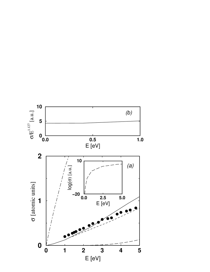
Figure 3: The total cross section $\sigma(E)$ for the electron-impact ionization of atomic hydrogen as a function of the excess energy $E$. The solid (long dashed) curve shows the results for $\sigma(E)$ when treating the two continuum electrons according to the DS3C theory (3C model) whereas the dashed dotted curve denotes the results of the independent Coulomb particles model (see text). Results of the CCC method are also included (short dashed curve). Experimental data are due to Shah et al. [32]. The inset in the panel (a) shows the results of the 3C theory on a logarithmic scale. In the upper panel (b) the quantity $\sigma(E)/E^{1.127}$ is depicted as a function of $E$ as evaluated using $\Psi_{\rm DS3C}$.

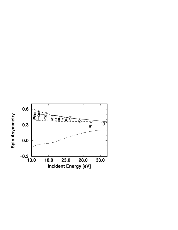
Figure 4: The spin asymmetry [Eq.(69)] in the total ionization cross section $\sigma(E)$ for the electron-impact ionization of atomic hydrogen. Results of the hidden crossing theory [25] (long dashed curve) and those of the CCC method [33] (solid curve) are depicted. Treating the final state according to the DS3C theory (3C theory) yields for the spin asymmetry the results shown by the short-dashed (dot-dashed) curve. The experimental data are due to Fletcher et al. [34] (full squares) and Crowe et al. [35] (open circles).

The Wannier treatment predicts the scaling behaviour of the cross section $\sigma(E)$, but it does not provide any information about the magnitude of $\sigma(E)$. That the magnitude is a very sensitive quantity is illustrated by the behaviour of the cross section in the independent Coulomb particle model which is obtained in our case by switching off the interaction between the two electrons in the final channel. In this case the cross section reveals a linear dependence on the excess energy, $\sigma(E)\propto E$ [42]. Although the latter dependence of $\sigma(E)$ does not deviate much from the Wannier threshold law ($\sigma(E)\propto E^{1.127}$) the absolute value of $\sigma(E)$ within the independent Coulomb particle model is largely overestimated [compare Fig.3]. If we employ the wave function $\Psi_{\rm DS3C}$, with the dynamical product charges described in the preceding sections we end up with results in good accord with the experimental measurements (cf. Fig.3). The absolute magnitude of the total cross section is satisfactorily reproduced when the DS3C model is employed. To examine the analytical behaviour of $\sigma(E)$ calculated using $\Psi_{\rm DS3C}$ we plot in Fig. 3(b) the quantity $\sigma(E)/E^{1.127}$. According to the Wannier-threshold law the latter quantity should be a constant function of $E$ and gives the absolute value of the cross section. As seen in Fig. 3(b) the Wannier threshold law is in fact reproduced by the cross section results of the $\Psi_{\rm DS3C}$ within a range of $E\in[0,0.5eV]$. For $E>0.5\ eV$ the analytical dependence of $\sigma(E)$ evaluated with $\Psi_{\rm DS3C}$ slowly deviates from the Wannier threshold law. When using the 3C method for the description of the two escaping electrons (${\cal A}={\rm I}$ in Eq.(52)) we obtain an analytical behaviour for $\sigma(E)$ which is not compatible with the Wannier theory. The absolute value for the total cross section is as well not reproduced by the 3C model, for the reasons discussed above. Also included in Fig.3 are the results of the convergent-close coupling method, CCC, [33]. The results of the CCC are in good agreement with the experimental $\sigma(E)$ for higher energies [33], however, close to threshold the evaluation of $\sigma(E)$ is limited by the computational resources as an ever increasing number of pseudo states is needed to achieve convergence.
In addition to the magnitude of the cross section, the spin asymmetry, $A$, offers a further way of probing the dynamical properties of the electron-impact ionization of atomic systems. The spin asymmetry $A$ is defined as

$$A(E):=\frac{\sigma^{s}(E)-\sigma^{t}(E)}{\sigma^{s}(E)+3\sigma^{t}(E)},$$ (69)

where $\sigma^{s}$ and $\sigma^{t}$ are the total ionization cross sections for singlet and triplet scattering, respectively. The Wannier theory for threshold ionization predicts a constant value of $A$ with increasing excess energy but provides no information on the numerical value of $A$ [43]. Measurements of $A$ at threshold reveals a slightly positive slope of the spin asymmetry with increasing excess energies [44]. In Fig.4 the results for $A$ are shown in the case where the two-electron continuum final state is described by the 3C theory and by $\Psi_{\rm DS3C}$. Also depicted in Fig.4 are the results of the CCC approach [33] and the method using hidden-crossing theory [25]. Although all theories, except for the 3C model, are in reasonable agreement with experimental finding the positive slope of $A$ at threshold is not reproduced.

Neglect of the short-ranged part of the Hamiltonian $H_{\it in}$ and $H_{\it mix}$, i.e. using the 3C model, results in a completely wrong behaviour of the calculated spin asymmetry. With increasing excess energy the inner region of the Hilbert space becomes of less importance for the present reaction and the results of the 3C method become more and more in better agreement with the experimental data.

We note here that since the spin asymmetry is a ratio of cross sections it is expected that the spin asymmetry is rather sensitive to the detailed of the radial part of the wave functions. From the agreement between the experiment and the DS3C theory observed in Fig. 4 we conclude that the radial part of $\Psi_{\rm DS3C}$ is well behaved at lower excess energies and that the short-range parts of the total Hamiltonian $H_{\it int}$ and $H_{\it mix}$ plays a dominate role at lower energies, as far as the value and the behaviour of the spin asymmetry are concerned.

4 Correlated states of N charged particles

In the preceding sections we considered the two and three-body continuum spectrum. Unfortunately, the curvilinear coordinate system (32,33) used for the three-body problem does not have a straightforward generalization to the $N$ body case. Therefore we will treat the problem of $N$ charged particles at energies above the complete fragmentation threshold within a reference frame spanned by a set of Jacobi coordinates. The problem becomes more transparent if we consider $N-1$ particles with equal masses (and with charges $z_{j},\ j\in[1,N-1]$) that move in the Coulomb field of a residual massive charge $z$. The mass $M$ of the charge $z$ is assumed to be much larger than $m$ ($M\gg m$). Neglecting terms of the order $m/M$ the centre-of-mass system and the laboratory frame of reference can be chosen to be identical. The non-relativistic time-independent Schrödinger equation of the $N$-body system can then be formulated in the relative-coordinate representation as

$$\left[H_{0}+\sum^{N}_{j=1}\frac{zz_{j}}{r_{j}}\ +\sum^{N}_{\stackrel{{\scriptstyle i,j}}{{j>i=1}}}\frac{z_{i}z_{j}}{r_{ij}}-E\right]\ \Psi({\bf r}_{1},\cdots,{\bf r}_{N})=0\ \$$ (70)

where ${\bf r}_{j}$ is the position of particle $j$ with respect to the residual charge $z$ and ${\bf r}_{ij}:={\bf r}_{i}-{\bf r}_{j}$ denotes the relative coordinate between particles $i$ and $j$ . The kinetic energy operator $H_{0}$ has the form (in the limit $m/M\to 0$) $H_{0}=-\sum_{\ell=1}^{N}\Delta_{\ell}/2m$ where $\Delta_{\ell}$ is the Laplacian with respect to the coordinate ${\bf r}_{\ell}$. We note here that for a system of general masses the problem is complicated by an additional mass-polarization term which arises in Eq.  (70). Upon introduction of $N$-body Jacobi coordinates, $H_{0}$ becomes diagonal, however, the potential terms acquire a much more complex form.
Assuming the continuum particles to escape with relative asymptotic momenta ${\bf k}_{j}$ (with respect to the charge $z$) it has been suggested in Ref.  [2], due to unpublished work by Redmond, that for large interparticle distances the wave function $\Psi({\bf r}_{1},\cdots,{\bf r}_{N})$ takes on the form

$$\smash{\lim_{\stackrel{{\scriptstyle r_{lm}\to\infty}}{{r_{n}\to\infty}}}}\Psi({\bf r}_{1},\cdots,{\bf r}_{N})\to(2\pi)^{-3N/2}\prod_{s=1}^{N}\bar{\xi}_{s}({\bf r}_{s})\psi_{s}({\bf r}_{s})\ \prod_{\stackrel{{\scriptstyle i,j=1}}{{j>i}}}^{N}\psi_{ij}({\bf r}_{ij})\ ,$$ (71)

where the functions $\bar{\xi}_{j}({\bf r}_{j}),\ \psi_{j}({\bf r}_{j}),\ \psi_{ij}({\bf r}_{ij})$ are defined as

$$\bar{\xi}_{j}({\bf r}_{j}) := \exp(i{\bf k}_{j}\cdot{\bf r}_{j})$$ (72)

$$\psi_{j}({\bf r}_{j}) := \exp\left[\mp i{\alpha}_{j}\ln(k_{j}\ r_{j}\pm{\bf k}_{j}\cdot{\bf r}_{j})\frac{}{}\right]\ ,$$ (73)

$$\psi_{ij}({\bf r}_{ij}) := \exp\left[\mp i{\alpha}_{ij}\ln(k_{ij}\ r_{ij}\pm{\bf k}_{ij}\cdot{\bf r}_{ij})\frac{}{}\right]\ .\$$ (74)

The $+$ and $-$ signs refer to outgoing and incoming boundary conditions, respectively, and ${\bf k}_{ij}$ is the momentum conjugate to ${\bf r}_{ij}$, i. e. ${\bf k}_{ij}:=({\bf k}_{i}-{\bf k}_{j})/2$. The Sommerfeld-parameters ${\alpha}_{j},{\alpha}_{ij}$ are given by

$${\alpha}_{ij}=\frac{z_{i}z_{j}}{v_{ij}},\hskip 28.45274pt{\alpha}_{j}=\frac{zz_{j}}{v_{j}}.\$$ (75)

In Eq.  (75) $v_{j}$ denotes the velocity of particle $j$ relative to the residual charge whereas ${\bf v}_{ij}:=\bf{v}_{i}-\bf{v}_{j}$. In this work we restrict the considerations to outgoing-wave boundary conditions. The treatment of incoming-wave boundary conditions runs along the same lines. The total energy of the system $E$ is given by

$$E=\sum_{l=1}^{N}E_{l},\ \mbox{ where }\ E_{l}=\frac{k^{2}_{l}}{2m}.$$ (76)

To derive asymptotic scattering states in the limit of large inter-particle separations and their propagations to finite distances we assume for $\Psi({\bf r}_{1},\cdots,{\bf r}_{N})$ the ansatz

$$\Psi({\bf r}_{1},\cdots,{\bf r}_{N})={\cal N}\Phi_{I}({\bf r}_{1},\cdots,{\bf r}_{N})\Phi_{II}({\bf r}_{1},\cdots,{\bf r}_{N})\chi({\bf r}_{1},\cdots,{\bf r}_{N})$$ (77)

where $\Phi_{I},\ \Phi_{II}$ are appropriately chosen functions, ${\cal N}$ is a normalization constant and $\chi({\bf r}_{1},\cdots,{\bf r}_{N})$ is a function of an arbitrary form. The function $\Phi_{I}$ is chosen to describe the motion of $N$-independent Coulomb particles moving in the field of the charge $z$ at the total energy $E$, i. e.  $\Phi_{I}$ is determined by the differential equation

$$\left(H_{0}+\sum_{j=1}^{N}\frac{zz_{j}}{r_{j}}-E\right)\Phi_{I}({\bf r}_{1},\cdots,{\bf r}_{N})=0.$$ (78)

Since we are interested in scattering solutions with outgoing-wave boundary conditions which describe $N$-particles escaping with asymptotic momenta ${\bf k}_{j},\ j\in[1,N]$, it is appropriate to factor out the plane-wave part and write for $\Phi_{I}$

$$\Phi_{I}({\bf r}_{1},\cdots,{\bf r}_{N})=\overline{\Phi}_{I}({\bf r}_{1},\cdots,{\bf r}_{N})\prod_{j=1}^{N}\bar{\xi}_{j}({\bf r}_{j}).$$ (79)

Upon substitution of the ansatz (79) into Eq.  (78) it is readily concluded that Eq.  (78) is completely separable and the regular solution $\Phi_{I}$ can be written in closed form

$$\Phi_{I}({\bf r}_{1},\cdots,{\bf r}_{N})=\prod_{j=1}^{N}\bar{\xi}_{j}({\bf r}_{j})\varphi_{j}({\bf r}_{j})$$ (80)

where $\varphi_{j}({\bf r}_{j})$ is a confluent-hypergeometric function in the notation of Ref.  [46]

$$\varphi_{j}({\bf r}_{j})=\ _{1}F_{1}[\alpha_{j},1,-i(k_{j}r_{j}+{\bf k}_{j}\cdot{\bf r}_{j})].$$ (81)

The function $\Phi_{I}$ describes the motion of the continuum particles in the extreme case of very strong coupling to the residual ion, i. e.  $|zz_{j}|\gg|z_{j}z_{i}|;\ \forall\ i,j\in[1,N]$. In order to incorporate the other extreme case of strong correlations among the continuum particles ($|z_{j}z_{i}|\gg|zz_{j}|;\ \forall\ i,j\in[1,N]$) we choose $\Phi_{II}$ to possess the form

$$\Phi_{II}({\bf r}_{1},\cdots,{\bf r}_{N})=\overline{\Phi}_{II}({\bf r}_{1},\cdots,{\bf r}_{N})\prod_{j=1}^{N}\bar{\xi}_{j}({\bf r}_{j})$$ (82)

with

$$\overline{\Phi}_{II}({\bf r}_{1},\cdots,{\bf r}_{N}):=\prod_{j>i=1}^{N}\varphi_{ij}({\bf r}_{ij})$$ (83)

where $\varphi_{ij}({\bf r}_{ij}):=\ _{1}F_{1}[\alpha_{ij},1,-i(k_{ij}r_{ij}+{\bf k}_{ij}\cdot{\bf r}_{ij})]$. It is straightforward to show that the expression $\varphi_{ij}({\bf r}_{ij})\prod_{l=1}^{N}\bar{\xi}_{l}({\bf r}_{l})$ solves for the Schrödinger Eq.  (70) in the case of extreme correlations between particle $i$ and particle $j$ , i. e.  $|zz_{l}|\ll|z_{i}z_{j}|\gg|z_{m}z_{n}|,\ \forall\ l,m,n\neq i,j$. In terms of differential equations this means

$$\left(H_{0}+\frac{z_{i}z_{j}}{r_{ij}}-E\right)\varphi_{ij}({\bf r}_{ij})\prod_{j=1}^{N}\bar{\xi}_{j}({\bf r}_{j})=0.$$ (84)

It should be stressed, however, that the function (82) does not solve for Eq.  (70) in case of weak coupling to the residual ion ($z\to 0$), but otherwise comparable strength of correlations between the continuum particles. This is due to the fact that two-body subsystems formed by the continuum particles are coupled to each other. To derive an expression for this coupling term we note first that

$$\Delta_{m}\overline{\Phi}_{II} = \sum_{l=1}^{m-1}\Delta_{m}\varphi_{lm}\prod_{\stackrel{{\scriptstyle j>i}}{{i\neq l}}}^{N}\varphi_{ij}\ +\ \sum_{n=m+1}^{N}\Delta_{m}\varphi_{mn}\prod_{\stackrel{{\scriptstyle j>i}}{{j\neq n}}}^{N}\varphi_{ij}+A_{m},\hskip 28.45274ptm\in[1,N]$$ (85)

where the differential operator $A_{m}$ has the form

$$A_{m} = 2\sum_{l=1}^{m-1}\left[({\bf\nabla}_{m}\varphi_{lm})\cdot(\sum_{n=m+1}^{N}{\bf\nabla}_{m}\varphi_{mn})\right]\prod_{\stackrel{{\scriptstyle j>i}}{{j\neq n,i\neq l}}}^{N}\varphi_{ij}$$ (86)

$$+\sum_{l=1}^{m-1}\left[({\bf\nabla}_{m}\varphi_{lm})\cdot(\sum_{l\neq s=1}^{m-1}{\bf\nabla}_{m}\varphi_{sm})\right]\prod_{\stackrel{{\scriptstyle j>i}}{{s\neq i\neq l}}}^{N}\varphi_{ij}$$

$$+\sum_{n=m+1}^{N}\left[({\bf\nabla}_{m}\varphi_{mn})\cdot(\sum_{\stackrel{{\scriptstyle t=m+1}}{{t\neq n}}}^{N}{\bf\nabla}_{m}\varphi_{mt})\right]\prod_{\stackrel{{\scriptstyle j>i}}{{j\neq t\neq n}}}^{N}\varphi_{ij}\hskip 28.45274ptm\in[1,N].$$

To obtain the differential operator which couples the two-body subsystems in absence of the charge $z$ we neglect in (70) the interactions between the residual charge and the continuum particles ($z=0$) and substitute the function (82) into Eq.  (70). Making use of the relation (85) it is straightforward, however cumbersome, to show that the coupling term which prevent separability has the form

$$A=\sum_{m=1}^{N}A_{m}.$$ (87)

Eqs. (86,87) warrant commented upon: The term $A_{m}$ is a mixing operator. It couples an individual two-body subsystem formed by two continuum particles to all other two-body subsystems formed by the continuum particles in absence of the residual ion. Hence it is clear that all the terms in the sum (86) vanishes for the case of three-body system since in this case only one two-body system does exist in the field of the residual charge. The second remark concerns the structure of $A_{m}$ and hence $A$. From Eq.  (85) it is evident that the remainder term (86) is part of the kinetic energy operator. Thus it is expected that, under certain circumstances, this term has a finite range which indicates that asymptotic separability, in the sense specified below, does exist for many-body continuum Coulomb systems. In fact, as the functional form of $\varphi_{ij}({\bf r}_{ij})$ is known the term $A$ can be calculated explicitely which will be done below.
Now with $\Phi_{I}$ and $\Phi_{II}$ have been determined, the exact wave function (77) is given by the expression $\chi({\bf r}_{1},\cdots,{\bf r}_{N})$. Upon substitution of the expressions (82,80) into the ansatz (77) and inserting in the Schrödinger equation (70) a differential equation for the determination of $\chi({\bf r}_{1},\cdots,{\bf r}_{N})$ is derived

$$\left\{H_{0}-\frac{A}{\overline{\Phi}_{II}}-\sum_{\ell=1}^{N}\left[({\bf\nabla}_{\ell}\ln\Phi_{I}\ +\ {\bf\nabla}_{\ell}\ln\Phi_{II})\cdot{\bf\nabla}_{\ell}\frac{}{}\right.\right.$$

$$\left.\left.+({\bf\nabla}_{\ell}\ln\Phi_{I})\cdot({\bf\nabla}_{\ell}\ln\Phi_{II})\frac{}{}\right]+E\right\}\chi({\bf r}_{1},\cdots,{\bf r}_{N})=0\ .$$ (88)

From the derivation of the functions $\Phi_{I}$ and $\Phi_{II}$ [Eqs. (78,82)] it is clear that all long-range two-body Coulomb interactions have been already diagonalized by $\Phi_{I}$ and $\Phi_{II}$ because the total potential is exactly treated by these wave functions. Hence, the function $\chi$, to be determined here, contains information on many-body couplings, which are, under certain conditions (see below), of finite range. To explicitely show that, and due to flux arguments we write the function $\chi$ in the form

$$\chi({\bf r}_{1},\cdots,{\bf r}_{N})=\prod_{j=1}^{N}{\bar{\xi}}^{*}({\bf r}_{j})[1-f({\bf r}_{1},\cdots,{\bf r}_{N})]$$ (89)

where $f({\bf r}_{1},\cdots,{\bf r}_{N})$ is a function of an arbitrary structure. Inserting the form (89) into Eq.  (88) we arrive, after much differential analysis, at the inhomogeneous differential equation

$$\left\{H_{0}-\sum_{\ell=1}^{N}\left[{\bf\nabla}_{\ell}(\ln\Phi_{I}\ +\ \ln\Phi_{II})+i{\bf k}_{\ell}\right]\cdot{\bf\nabla}_{\ell}\right\}f+{\cal R}(1-f)=0$$ (90)

where the inhomogeneous term ${\cal R}$ is given by

$${\cal R}:=\sum_{m=1}^{N} \left\{({\bf\nabla}_{m}\ln\overline{\Phi}_{I})\cdot({\bf\nabla}_{m}\ln\overline{\Phi}_{II})+\sum_{l=1}^{m-1}\sum_{p=m+1}^{N}({\bf\nabla}_{m}\ln\varphi_{lm})\cdot({\bf\nabla}_{m}\ln\varphi_{mp})\right.$$ (91)

$$\left.+\frac{1}{2}\sum_{l=1}^{m-1}\sum_{s\neq l}^{m-1}({\bf\nabla}_{m}\ln\varphi_{lm})\cdot({\bf\nabla}_{m}\ln\varphi_{sm})\right.$$

$$+\left.\frac{1}{2}\sum_{n=m+1}^{N}\sum_{n\neq q=m+1}^{N}({\bf\nabla}_{m}\ln\varphi_{mn})\cdot({\bf\nabla}_{m}\ln\varphi_{mq})\right\}.$$

It is the inhomogeneous term ${\cal R}$ which contains the coupling between all individual two-particle subsystems. For example the first term in Eq. (91) describes the coupling of a two-body subsystems formed by particles $i$ and $j$ to all two-body subsystems formed by the individual continuum particles and the residual ion. The second term originates from (87) and, as explained above, is a measure for the coupling among two-body subsystems of the continuum particles (in absence of $z$). To these couplings to be negligible the norm of the term ${\cal R}$ must be small. For get some insight into the functional form of ${\cal R}$, given by (91), we note that

$${\bf\nabla}_{\ell}\ln\overline{\Phi}_{I}=\alpha_{\ell}k_{\ell}\ {\bf F}_{\ell}({\bf r}_{\ell})$$ (92)

where

$${\bf F}_{\ell}({\bf r}_{\ell}) := {\frac{\mbox{}_{1}F_{1}\left[1+i\alpha_{\ell},\ 2,\ -i(k_{\ell}\ r_{\ell}+{{\bf k}_{\ell}}\cdot{{\bf r}_{\ell}})\ \right]}{{}_{1}F_{1}\left[i\alpha_{\ell},\ 1,\ -i(k_{\ell}\ r_{\ell}+{{\bf k}_{\ell}}\cdot{{\bf r}_{\ell}})\ \right]}\ ({\bf\hat{k}}_{\ell}+{\bf\hat{r}}_{\ell})}\ .\$$ (93)

In addition we remark that

$${\bf\nabla}_{m}\ln\overline{\Phi}_{II} = \sum_{n=m+1}^{N}{\bf\nabla}_{m}\ln\varphi_{mn}+\sum_{l=1}^{m-1}{\bf\nabla}_{m}\ln\varphi_{lm}$$ (94)

$$= \sum_{n=m+1}^{N}\alpha_{mn}k_{mn}{\bf F}_{mn}({\bf r}_{mn})-\sum_{l=1}^{m-1}\alpha_{lm}k_{lm}{\bf F}_{lm}({\bf r}_{lm})$$

where

$${\bf F}_{ij}({\bf r}_{ij}) := {\frac{\mbox{}_{1}F_{1}\left[1+i\alpha_{ij},\ 2,\ -i(k_{ij}\ r_{ij}+{{\bf k}_{ij}}\cdot{{\bf r}_{ij}})\ \right]}{{}_{1}F_{1}\left[i\alpha_{ij},\ 1,\ -i(k_{ij}\ r_{ij}+{{\bf k}_{ij}}\cdot{{\bf r}_{ij}})\ \right]}\ ({\bf\hat{k}}_{ij}+{\bf\hat{r}}_{ij})}\ .\$$ (95)

Thus, the behavior of the coupling term ${\cal R}$ is controlled by the generalized functions ${\bf F}_{ij}({\bf r}_{ij}),\ {\bf F}_{l}({\bf r}_{l})$ since Eq.  (91) can be written in the form

$${\cal R}:=\sum_{m=1}^{N} \left\{\alpha_{m}k_{m}{\bf F}_{m}({\bf r}_{m})\cdot\left[\sum_{n=m+1}^{N}\alpha_{mn}k_{mn}{\bf F}_{mn}({\bf r}_{mn})-\sum_{s=1}^{m-1}\alpha_{sm}k_{sm}{\bf F}_{sm}({\bf r}_{sm})\right]\right.$$ (96)

$$- \sum_{l=1}^{m-1}\sum_{p=m+1}^{N}\alpha_{lm}\alpha_{mp}k_{lm}k_{mp}{\bf F}_{lm}\cdot{\bf F}_{mp}+\frac{1}{2}\sum_{l=1}^{m-1}\sum_{s\neq l}^{m-1}\alpha_{lm}\alpha_{sm}k_{lm}k_{sm}{\bf F}_{lm}\cdot{\bf F}_{sm}$$

$$+\left.\frac{1}{2}\sum_{n=m+1}^{N}\sum_{n\neq q=m+1}^{N}\alpha_{mn}\alpha_{mq}k_{mn}k_{mq}{\bf F}_{mn}\cdot{\bf F}_{mq}\right\}.$$

The simplest approximation is to neglect the term ${\cal R}$ altogether. In this case the function $f=0$ solves for the equation (90). Then, the solution of Eq.  (70) takes on the approximate form

$$\Psi({\bf r}_{1},\cdots,{\bf r}_{N})\approx{\cal N}\prod_{m>l,j=1}^{N}\bar{\xi}_{j}({\bf r}_{j})\varphi_{j}({\bf r}_{j})\varphi_{lm}({\bf r}_{lm}).$$ (97)

Thus, the justification of the approximation (97) reduces to the validity of neglecting the inhomogeneous term (96). One region in which this term can be disregarded is the asymptotic region of large inter-particle separations. This is immediately deduced from the asymptotic behavior of the generalized functions ${\bf F}_{ij}({\bf r}_{ij}),\ {\bf F}_{l}({\bf r}_{l})$ which dictate the asymptotic properties of ${\cal R}$, as readily concluded from Eq.  (96). From the asymptotic expansion of the hypergeometric functions [46] we infer that

$$\lim_{r_{ij}\to\infty}|{\bf F}_{ij}({\bf r}_{ij})|\ \to\ \left|\ \frac{{\bf\hat{k}}_{ij}+{\bf\hat{r}}_{ij}}{{\bf k}_{ij}\cdot({\bf\hat{k}}_{ij}+{\bf\hat{r}}_{ij})\ r_{ij}}\ \right|\ +\ {\cal O}\left(|k_{ij}\ r_{ij}+{\bf k}_{ij}\cdot{\bf r}_{ij}|^{-2}\right)\ .\$$ (98)

A asymptotic relation similar to Eq.  (98) holds for ${\bf F}_{l}({\bf r}_{l})$. It should be noted that the functions ${\bf F}_{ij}({\bf r}_{ij}),\ {\bf F}_{l}({\bf r}_{l})$ have to be considered in a distributive (operator) sense which means that, asymptotically, only terms of ${\bf F}_{ij},{\bf F}_{l}$ which fall off faster than the Coulomb potentials can be disregarded. Since ${\cal R}$ is essentially a sum of products of ${\bf F}_{ij},{\bf F}_{l}$ the expression ${\cal R}$ is of finite range, in the sense that it diminishes faster than the Coulomb potential in the asymptotic regime, only in the case where all particles are far apart from each other, i. e.

$$\lim_{\stackrel{{\scriptstyle{r_{ij}\to\infty}}}{{r_{l}\to\infty}}}{\cal R}\ \to\ {\cal O}\left(|k_{ij}\ r_{ij}+{\bf k}_{ij}\cdot{\bf r}_{ij}|^{-2},|k_{l}\ r_{l}+{\bf k}_{l}\cdot{\bf r}_{l}|^{-2}\right)\ \hskip 8.5359pt\forall\hskip 5.69046ptj>i,l\in[1,N].\$$ (99)

Therefore, in the limit (99), the term ${\cal R}$ can be asymptotically neglected and the approximation (97) is justified. In fact, it is straightforward to show that the wave function (97) tends to the asymptotic form (71) in the limit of large inter-particle separations which proves the assumption made in Ref.  [2]. However, if two particles are close together, regardless of whether all other particles are well separated, the coupling term is of infinite range, as seen from Eqs. (98,96). In this case the relation (99) does not hold. Consequently, the wave function (97) is not an exact asymptotic eigenfunction of the total Hamiltonian in this limit. It is important to note that the limit Eq. (99) is energy dependent. With increasing momenta of the escaping particles the asymptotic region, i. e. the limit Eq. (99), is reached faster. In other words, at a certain inter-particle separations, the remainder term ${\cal R}$, which has been neglected to arrive at the approximate form (97), diminishes with increasing velocities of the emerging particles. In this sense the approximation leading to the wave function (97) is a high energy approximation.

4.1 The two-body cusp conditions

In the preceding section it has been shown that the approximation (97) is, to leading order, exact for large particles separation. In addition, it is concluded below that this function exhibits a behavior compatible with equation (70) at all two-body coalescence points $r_{ij}\to 0,r_{l}\to 0,\ j>i,l\in[1,N]$. To guarantee regular behavior of the wave function at these collision points, at which the corresponding Coulomb two-body potential is divergent, the solution $\Psi({\bf r}_{1},\cdots,{\bf r}_{N})$ of Eq.  (70) must satisfy the Kato cusp conditions [45, 47] (provided the solution does not vanish at these points). At a collision point $r_{i}\to 0$ these conditions are

$$\left[\frac{\partial\ \tilde{\Psi}({\bf r}_{1},\cdots,{\bf r}_{N})}{\partial\ r_{i}}\right]_{r_{i}=0} = k_{i}\alpha_{i}\Psi({\bf r}_{1},\cdots,r_{i}=0,\cdots,{\bf r}_{N})\hskip 14.22636pt$$ (100)

$$\forall\hskip 5.69046pt(r_{i}/r_{j})\to 0,(r_{i}/r_{lm})\to 0;\ m>l,\ i\neq j\in[1,N]\ .\$$

The quantity $\tilde{\Psi}({\bf r}_{1},\cdots,{\bf r}_{N})$ is the wave function ${\Psi}({\bf r}_{1},\cdots,{\bf r}_{N})$ averaged over a sphere of small radius $r_{\delta}\ll 1$ around the singularity $r_{i}=0$. A relation similar to Eq.  (100) holds in the case of the coalescence points $r_{ij}\to 0$. To prove that the wave function (97) does satisfy the conditions (100) we linearize $\Psi({\bf r}_{1},\cdots,{\bf r}_{N})$ around $r_{i}=0$ and average over a sphere of small radius $r_{\delta}\ll 1$ to arrive at

$$\tilde{\Psi}({\bf r}_{1},\cdots,{\bf r}_{N}) = {\cal N}\ D({\bf r}_{i})\prod_{\stackrel{{\scriptstyle i\neq j=1}}{{l>m}}}^{N}\bar{\xi}_{j}\varphi_{j}({\bf r}_{j})\varphi_{lm}({\bf r}_{lm}),\ \epsilon_{ilm}\neq 0$$ (101)

where

$$D({\bf r}_{i}) = \frac{2\pi}{4\pi r_{\delta}^{2}}\int_{-1}^{1}\!r_{\delta}^{2}\ d\cos\theta\ \left[\ \frac{}{}1+ik_{i}\cos\theta+{\alpha}_{i}k_{i}\ r_{i}(1+\cos\theta)\ \right]$$ (102)

$$= 1+{\alpha}_{i}\ k_{i}\ r_{i}\ .\$$

To arrive at Eq.  (102) one takes the $z-$axes as ${\bf k}_{i}$ and define $\cos\theta={\bf\hat{k}}_{i}\cdot{\bf\hat{r}}_{i}$. From Eqs. (102,101) it is obvious that

$$\left[\frac{\partial\ \tilde{\Psi}({\bf r}_{1},\cdots,{\bf r}_{N})}{\partial\ r_{i}}\right]_{r_{i}=0} = \alpha_{i}k_{i}\ {\cal N}\prod_{\stackrel{{\scriptstyle i\neq j=1}}{{l>m}}}^{N}\bar{\xi}_{j}\varphi_{j}({\bf r}_{j})\varphi_{lm}({\bf r}_{lm})$$ (103)

$$= \alpha_{i}k_{i}{\Psi}({\bf r}_{1},\cdots,r_{i}=0,\cdots,{\bf r}_{N}),\ \epsilon_{ilm}\neq 0.$$

In deriving Eq.  (103) we made use of the fact that in the limit $(r_{i}/r_{ij}\to 0)$ the distance $r_{ij}$ tends to $r_{j}$. The proof that the wave function (97) fulfills the cusp conditions at the collision points of two continuum particles ($r_{ji}\to 0$) runs along the same lines. Finally, we remark that the wave function (97) is not compatible with the expansion of the exact solution of the Schrödinger equation (70) at the three-body collision points (e.g. $r_{i}\to 0$ and $r_{j}\to 0,j\neq i$) since in this case the exact wave function is known to satisfy a Fock expansion [15] in the coordinate $\rho:=\sqrt{(r_{i}^{2}+r_{j}^{2})}$ which contains, in addition to powers in $\rho$, logarithmic terms in $\rho$ whereas the wave function (97) possesses a regular power-series expansion around $r_{i}\to 0$ and $r_{j}\to 0$.

4.2 Normalization

The knowledge of the normalization factor ${\cal N}$ of the wave function (97) is imperative for the evaluation of scattering amplitudes using the wave function (97) as a representation of scattering states. In principle, ${\cal N}$ is derived from a $3N$-dimensional integral over the norm of the function (97) which, for large $N$, is an inaccessible task. Thus for the determination of ${\cal N}$ we resort to the requirement that the flux through an asymptotic manifold defined by a constant large inter-particle separations should be the same in the case of the wave function (97) and a normalized plane-wave representation of the scattering state, i. e.

$${\bf J}_{PW}={\bf J}_{\Psi}$$ (104)

where the plane-wave flux is given by

$${\bf J}_{PW} = -\frac{i}{2}(2\pi)^{-3N}\left[\prod_{l}^{N}\bar{\xi}^{*}_{l}({\bf r}_{l}){\bf\nabla}\prod_{l}^{N}\bar{\xi}_{l}({\bf r}_{l})-\prod_{l}^{N}\bar{\xi}_{l}({\bf r}_{l}){\bf\nabla}\prod_{l}^{N}\bar{\xi}^{*}_{l}({\bf r}_{l})\right]$$ (105)

$$= (2\pi)^{-3N}\sum_{l=1}^{N}{\bf k}_{l}.$$

In Eq. (105) the total gradient ${\bf\nabla}:=\sum_{l=1}^{N}{\bf\nabla}_{l}$ has been introduced. To evaluate the flux generated by the wave function (97) we note that, by taking advantage of Eqs. (92,94), we can write for the total gradient of the wave function (97)

$${\bf\nabla}\Psi:=P{\cal N}\sum_{m=1}^{N} \left\{i{\bf k}_{m}\Psi+\alpha_{m}k_{m}{\bf F}_{m}{\Psi}\ +\ \left[\sum_{n=m+1}^{N}\alpha_{mn}k_{mn}\overline{\bf F}_{mn}({\bf r}_{mn})\prod_{\stackrel{{\scriptstyle j>i}}{{j\neq n}}}^{N}\varphi_{ij}\right.\right.$$ (106)

$$\left.\left.-\sum_{l=1}^{m-1}\alpha_{lm}k_{lm}\overline{\bf F}_{lm}({\bf r}_{lm})\prod_{\stackrel{{\scriptstyle j>i}}{{i\neq l}}}^{N}\varphi_{ij}\right]\prod_{s=1}^{N}\bar{\xi}_{s}({\bf r}_{s})\varphi_{s}({\bf r}_{s})\right\}$$

where $\overline{\bf F}_{mn}$ is given by ${\bf F}_{mn}\varphi_{mn}$. The decisive point now is that since we are considering the flux at large interparticle distances only the first term of Eq.  (106) is relevant. This is readily deduced from Eqs. (93,95) which state that all other terms in Eq.  (106), except for the first term, can be neglected asymptotically. Note in this context that terms in the wave function which are asymptotically of the order ${\cal O}(1/r_{j},1/r_{lm})$ correspond to parts of the Hamiltonian falling off faster than the Coulomb potentials and hence can be disregarded in the asymptotic regime. Now making use of the asymptotic expansion of the confluent hypergeometric function [46] and taking leading order in the interparticle distances the flux ${\bf J}_{\Psi}$ can de deduced

$${\bf J}_{\Psi}={\cal N}^{2}\prod_{j=1}^{N}\frac{\exp(\pi\alpha_{j})}{\Gamma(1-i\alpha_{j})\Gamma^{*}(1-i\alpha_{j})}\prod_{m>l=1}^{N}\frac{\exp(\pi\alpha_{lm})}{\Gamma(1-i\alpha_{lm})\Gamma^{*}(1-i\alpha_{lm})}\sum_{n=1}^{N}{\bf k}_{n}$$ (107)

where $\Gamma(x)$ is the Gamma function. From Eqs. (104,105,107) it follows that

$${\cal N}=(2\pi)^{-3N/2}\prod_{j=1,m>l=1}^{N}\exp[-\pi(\alpha_{lm}+\alpha_{j})/2]\Gamma(1-i\alpha_{j})\Gamma(1-i\alpha_{lm}).$$ (108)

For two charged particles moving in the field of a heavy nucleus the wave function (97) with the normalization, given by Eq.  (108), simplifies to the three-body wave function that has been discussed in the previous section.

5 Green function theory of finite correlated systems

In the preceding sections we investigated the two, three and $N$-body correlated scattering states. With increasing number of particles the treatment becomes more complex and a methodology different from the wave function technique is more appropriate. A method which is widely used in theoretical physics is the Green function approach which we will follow up in this section.

For a canonical ensemble, we seek a non-perturbative method which allows to distribute systematically the total energy between the potential and the kinetic energy parts. This is achieved by the development of an incremental method in which the $N$ correlated particle system is mapped exactly onto a set of systems in which only $N-M$ particles are interacting ($M\in[1,N-2]$), i.e. in which the potential energy part is damped. (In contrast to re-normalization group theory we do not reduce the strength of interactions, but the number of them). This is particularly interesting from a thermodynamic point of view since for a number of thermodynamic properties the kinetic energy contributions can be separated out from the potential energy parts, as shown in the next section for the internal energy. By virtue of the present method the potential energy part is systematically reduced.

For a formal development let us consider a nonrelativistic system consisting of $N$ interacting particles. We assume the total potential to be of the class $U^{(N)}=\sum_{j>i=1}^{N}v_{ij}$ without any further specification of the individual potentials $v_{ij}$. For three-body potentials the development of the theory proceeds along the same lines.

The potential $U^{(N)}$ satisfies the recurrence relations

$$U^{(N)} = \frac{1}{N-2}\sum_{j=1}^{N}u_{j}^{(N-1)},$$ (109)

$$u_{j}^{(N-1)} = \frac{1}{N-3}\sum_{k=1}^{N-1}u^{(N-2)}_{jk},\,\,j\neq k,$$ (110)

where $u_{j}^{(N-1)}$ is the total potential of a system of $N-1$ interacting particles in which the $j$ particle is missing, i.e. in terms of the physical pair potentials $v_{mn}$, one can write $u_{j}^{(N-1)}=\sum_{m>n=1}^{N}v_{mn},\>m\neq j\neq n$.

The fundamental quantity that describes the microscopic properties of the $N$ body quantum system is the Green operator $G^{(N)}$ which is the resolvent of the total Hamiltonian. It can be deduced from the Lippmann Schwinger equation $G^{(N)}=G_{0}+G_{0}U^{(N)}G^{(N)}$ where $G_{0}$ is the Green operator of the non interacting $N$ body system. An equivalent approach to determine the dynamical behavior of a system is to derive the respective transition operator $T^{(N)}$ which satisfies the integral equation $T^{(N)}=U^{(N)}+U^{(N)}G_{0}T^{(N)}$. These integral equations for $G^{(N)}$ and $T^{(N)}$ provide a natural framework for perturbative treatments. However, for $N\geq 3$ the application of the above Lippmann Schwinger equations (and those for the state vectors) is hampered by mainly two difficulties: 1.) as shown in Refs. [48, 49] the Lippmann Schwinger equations for the state vectors do not have a unique solution, and 2.) as shown by Faddeev [50, 51, 52] the kernel of these integral equations $K=G_{0}U^{(N)}$ is not a square integrable operator for $N\geq 3$, i.e.  the norm $\|K\|=[{\rm Tr}(KK^{\dagger})]^{1/2}$ is not square integrable. The kernel $K$ is also not compact. The reason for this drawback is the occurrence of the so-called disconnected diagrams where one of the $N$ particles is a spectator, i.e. not correlated with the other $N-1$ particles. For the three-body problem Faddeev [50, 51] suggested alternative integral equations with square integrable kernel.

Our aim here is twofold: (a) We would like to derive non-perturbative integral equations that treat all $N$ particles on equal footing and are free from disconnected diagrams. (b) These equations should allow to obtain, in a computationally accessible manner, the solution of the correlated $N$ body problem from the solution when only $N-M$ particles are interacting (where $M\in[1,N-2]$).

According to the decomposition (109), the integral equation for the transition operator can be written as

$$T^{(N)} = \sum_{j=1}^{N}T^{(N-1)}_{j}$$ (111)

$$T^{(N-1)}_{j} = \tilde{u}_{j}^{(N-1)}+T^{(N)}G_{0}\tilde{u}_{j}^{(N-1)},\,\,j\in[1,N].$$

Here we introduced the scaled potential

$$\tilde{u}_{j}^{(N-1)}=\left(u_{j}^{(N-1)}\right)/(N-2).$$

The transition operator of the system, when $N-1$ particles are interacting via the scaled potential $\tilde{u}_{j}^{(N-1)}$, is

$$t^{(N-1)}_{j}=\tilde{u}_{j}^{(N-1)}+\tilde{u}_{j}^{(N-1)}G_{0}t^{(N-1)}_{j}.$$

With this relation Eq.(LABEL:tn1) can be reformulated as

$$T^{(N-1)}_{j} = t^{(N-1)}_{j}+t^{(N-1)}_{j}G_{0}T^{(N)}-$$

$$t^{(N-1)}_{j}G_{0}\left(\tilde{u}_{j}^{(N-1)}+\tilde{u}_{j}^{(N-1)}G_{0}T^{(N)}\right)$$

$$= t^{(N-1)}_{j}+t^{(N-1)}_{j}G_{0}\left(T^{(N)}-T^{(N-1)}_{j}\right)$$

$$= t^{(N-1)}_{j}+t^{(N-1)}_{j}G_{0}\sum_{k\neq j}^{N}T^{(N-1)}_{k}.$$

Eq.(LABEL:ex) can be expressed in a matrix form as follows

$$\left(\begin{array}[]{c}T^{(N-1)}_{1}\\ T^{(N-1)}_{2}\\ \vdots\\ T^{(N-1)}_{N-1}\\ T^{(N-1)}_{N}\end{array}\right) = \left(\begin{array}[]{c}t^{(N-1)}_{1}\\ t^{(N-1)}_{2}\\ \vdots\\ t^{(N-1)}_{N-1}\\ t^{(N-1)}_{N}\end{array}\right)+[{\bf K}^{(N-1)}]\left(\begin{array}[]{c}T^{(N-1)}_{1}\\ T^{(N-1)}_{2}\\ \vdots\\ T^{(N-1)}_{N-1}\\ T^{(N-1)}_{N}\end{array}\right).$$ (129)

The kernel $[{\bf K}^{(N-1)}]$ is a matrix operator and is given by

$$[{\bf K}^{(N-1)}]=\left(\begin{array}[]{ccccc}0&t^{(N-1)}_{1}&t^{(N-1)}_{1}&\lx@intercol\dotfill\hfil\hfil\lx@intercol&t^{(N-1)}_{1}\\ t^{(N-1)}_{2}&0&t^{(N-1)}_{2}&\lx@intercol\dotfill\hfil\hfil\lx@intercol&t^{(N-1)}_{2}\\ \lx@intercol\dotfill\hfil\hfil\lx@intercol\\ t^{(N-1)}_{N-1}&\lx@intercol\dotfill\hfil\hfil\lx@intercol&t^{(N-1)}_{N-1}&0&t^{(N-1)}_{N-1}\\ t^{(N-1)}_{N}&\lx@intercol\dotfill\hfil\hfil\lx@intercol&t^{(N-1)}_{N}&t^{(N-1)}_{N}&0\end{array}\right)G_{0}.$$ (135)

From Eq.(110) it is clear that $t_{j}^{(N-1)}$ can also be expressed in terms of the transition operators of the system where only $N-2$ particles are interacting:

$$t_{j}^{(N-1)}=\sum_{k\neq j}^{N-1}T^{(N-2)}_{k}.$$

The operators $T^{(N-2)}_{k}$ are deduced from Eq.(129) with $N$ being replaced by $N-1$.

From the relation $G^{(N)}=G_{0}+G_{0}T^{(N)}G_{0}$ we conclude that the Green operator of the interacting $N$ particle system has the form

$$G^{(N)}=G_{0}+\sum_{j=1}^{N}G^{(N-1)}_{j}.$$ (137)

The operators $G^{(N-1)}_{j}$ are related to the Green operators $g^{(N-1)}_{j}$ of the systems in which only $N-1$ particles are correlated by virtue of $\tilde{u}_{j}^{(N-1)}$. This interrelation is given via

$$\left(\begin{array}[]{c}G^{(N-1)}_{1}\\ G^{(N-1)}_{2}\\ \vdots\\ G^{(N-1)}_{N-1}\\ G^{(N-1)}_{N}\end{array}\right) = \left(\begin{array}[]{c}g^{(N-1)}_{1}-G_{0}\\ g^{(N-1)}_{2}-G_{0}\\ \vdots\\ g^{(N-1)}_{N-1}-G_{0}\\ g^{(N-1)}_{N}-G_{0}\end{array}\right)+[{\bf\tilde{K}}^{(N-1)}]\left(\begin{array}[]{c}G^{(N-1)}_{1}\\ G^{(N-1)}_{2}\\ \vdots\\ G^{(N-1)}_{N-1}\\ G^{(N-1)}_{N}\end{array}\right),$$ (153)

where $[{\bf\tilde{K}}^{(N-1)}]=G_{0}[{\bf\tilde{K}}^{(N-1)}]G_{0}^{-1}$. From Eqs.(129,153) we conclude that if the Green operator of the interacting $N-1$ body system is known (from other analytical or numerical procedures, e.g. from an effective field method, such as density functional theory) the Green operator of the $N$ particles can then be deduced by solving a set of $N$ linear, coupled integral equations (namely Eqs.(129,153)). According to the above equations, if only the solution of the $N-M$ problem is known where $M\in[1,N-2]$ we have to perform a hierarchy of calculations starting by obtaining the solution for the $N-M+1$ problem and repeating the procedure to reach the solution of the $N$ body problem.

At first sight the kernels of Eqs. (129,153) appear to have disconnected diagrams since they contain transition operators of systems where only $N-1$ particles are interacting and one particle is free (disconnected). It is, however, straightforward to show that any iteration of these kernels is free of disconnected terms (the disconnected terms occurs only in the off-diagonal elements of $[{\bf K}^{N-M}]$ and $[\tilde{\bf K}^{N-M}]$). For $N=3$ the present scheme reduces to the well-established Faddeev equations. As for the functional structure of the Eqs. (129,153) we remark that for the solution of the $N$ particle problem we need the (off-shell) transition operators of the $N-1$ subsystem. The interaction potentials do not appear in this formulation (in contrast to the Lippmann Schwinger approach). On the other hand the (on-shell) transition matrix elements can be determined experimentally. This fact becomes valuable when the potentials are not known.

5.1 Application to four-body systems

Over the years a substantial body of knowledge on the three-particle problem has been accumulated. In contrast, theoretical studies on the four-body problem are still scare due to computational limitations whereas an impressive amount of experimental data is already available [53, 54, 55, 56, 57]. Thus, it is desirable to apply the above procedure to the four-body system and to express its solution in terms of known solutions of the three-body problem. For $N=4$ the first iteration of Eq.(153) yields

$$G^{(4)}=\sum_{j=1}^{4}g^{(3)}_{j}-3G_{0}.$$ (154)

Here $g^{(3)}_{j}$ is the Green operator of the system where only three particles are interacting and can be taken from other numerical or analytical studies. This means, to a first order, methods treating the correlated three-body problem can be extended to deal with the four-body case using Eq.(154). We note that for the case of non-interacting system $g^{(3)}_{j}$ reduces to $g^{(3)}_{j}\equiv G_{0}$ and hence Eq.(154) reduces to $G^{(4)}=G_{0}$, as expected.

The Green function encompasses the complete spectrum of the many-body system, i.e. the wave function approach can be retrieved from the Green function. For example, Eq.(154) leads to an expression for the four-body state vector in the form

$$|\Psi^{(4)}\rangle = |\psi^{(3)}_{234}\rangle+|\psi^{(3)}_{134}\rangle+|\psi^{(3)}_{124}\rangle+|\psi^{(3)}_{123}\rangle-3|\phi^{(4)}_{\rm free}\rangle.$$ (155)

Here $|\psi^{(3)}_{ijk}\rangle$ is the state vector of the system in which the three particles $i,j$ and $k$ are interacting whereas $|\phi^{(4)}_{\rm free}\rangle$ is the state vector of the non-interacting four-body system. The state vectors $|\psi^{(3)}_{ijk}\rangle$ can be approximated by Eq.(53) or by the other procedures discussed in the preceding section on the three-body problem.

Since the state vector (155) is expressed as a sum of correlated three-body states, the evaluation of the four-body transition matrix elements for a specific reaction simplifies considerably. In addition, the spectral properties of a many-body interacting system can be obtained in a straightforward way from those for systems with a reduced number of interactions, for in this case the matrix elements of the total Green functions are expressed as sums of matrix elements of reduced Green functions, as evident from Eq.(154). This spectral feature can be exploited to study the thermodynamical properties of finite correlated systems.

6 Thermodynamics and phase transitions of interacting finite systems

To investigate the thermodynamical properties of $N$ interacting particle system we remark that at the critical point divergent thermodynamical quantities, such as the specific heat $C_{V}$ are obtained as a derivative with respect to the inverse temperature $\beta$ of the logarithm of the canonical partition function $Z(\beta)$,

$$C_{V}=\beta^{2}\partial^{2}_{\beta}\ln Z(\beta)=f(\beta,Z(\beta))/Z(\beta).$$

Here $f$ is some analytical function and for the Boltzmann constant we assume $k=1$.

Therefore divergences in the thermodynamic quantities, which signify phase transitions are connected to the zero points of $Z(\beta)$. These zero points are generally complex valued. Therefore an analytical continuation of $Z(\beta)$ to complex temperatures is needed.

The connection between the phase transitions and the complex zero points of the grand canonical partition function have been uncovered by Yang and Lee [58]. In this case one seeks an analytical continuation of the fugacity $z=\exp(\beta\mu)$ (here $\mu$ is the chemical potential) to the complex plane $z\to\Re(z)+i\Im(z)$. In the thermodynamic limit the zero points condense to lines. The transition points are the crossing points of these lines with the real fugacity axis.

Grossman et al. [59] generalized the concept of Yang and Lee to the canonical ensemble. In this case the inverse temperature $\beta=1/T$ is continued analytically to $\beta=\Re(\beta)+i\Im(\beta)$. The phase transitions are then the crossings of the zero points line of $Z(\beta)$ with the real $\beta$ axis. The advantage here is that a classification of the phase transitions can be given in terms of how the zero-points line do cross the real $\beta$ axis [59].

The crucial point is that in the thermodynamic limit $N\to\infty,\,V\to\infty$ and $v=V/N<\infty$ ($V$ is the volume) the zero points approach, to an infinitesimal small distance the real axis. For this reason, the characteristic phase-transition divergences appear in the thermodynamical quantities. For finite systems $Z(\beta)$ has only finite zero points that do not approach infinitely close the real axis. Therefore, the thermodynamic quantities show smooth peaks rather then divergences. The positions and widths of these peaks can be obtained from the real and imaginary parts of the zero points laying closest to the real axis [60].

To apply this method to correlated finite systems we need a representation of the canonical partition function that can then be continued analytically to the complex temperature plane.

The canonical partition function of a correlated system can be expressed in terms of the many-body Green function as

$$Z(\beta)=\int dE\;\Omega(E)\;e^{-\beta E}.$$ (156)

Here $\Omega(E)$ is the density of states which is related to imaginary part of the trace of $G^{(N)}$ via

$$\Omega(E)=-\frac{1}{\pi}\Im\,{\mathbf{Tr}}\,G^{(N)}(E).$$ (157)

From the Green function expansion Eq.(137) we deduce

$$Z(\beta) = -\frac{1}{\pi}\Im\int dE\;{\mathbf{Tr}}\,G^{(N)}(E)\;e^{-\beta E}$$ (158)

$$= Z_{0}(\beta)+\sum_{j=1}^{N}Z_{j}(\beta)$$

where

$$Z_{0}(\beta) = -\frac{1}{\pi}\Im\int dE\;{\mathbf{Tr}}\,G_{0}(E)\;e^{-\beta E}$$ (159)

$$Z_{j}(\beta) = -\frac{1}{\pi}\Im\int dE\;{\mathbf{Tr}}\,G_{j}^{(N-1)}(E)\;e^{-\beta E}.$$

To a first order $Z_{j}=Z_{j}^{(N-1)}-Z_{0}$ where $Z_{j}^{(N-1)}$ is the partition function of a system in which only $N-1$ particles are interacting. For the applications of the Grossmann method let us remark that $Z(\beta)$ is an integral function and can be expressed in a polynomial form. Recalling the analytical properties of meromorphic functions one can write $Z(\beta)$ in terms of its complex zero points as

$$Z(\beta)=Z(0)e^{\beta\frac{Z^{\prime}(0)}{Z(0)}}\>\prod^{\infty}_{k=1}\left(1-\frac{\beta}{\beta_{k}}\right)e^{\frac{\beta}{\beta_{k}}}.$$ (161)

7 Conclusions

In conclusions we reviewed recent advances in the analytical treatment of correlated few charged-particle systems. Starting from the two-body (Kepler) problem we discussed the mathematical and physical properties of a three-body system above the complete fragmentation threshold. Analytical approximate expressions for the three-body wave functions have been derived and employed for the calculations of transition matrix elements in atomic scattering experiments. The discussion has been extended to the case of $N$ charged particles in the continuum where $N$ particle wave functions have been derived and their mathematical features have been exposed. For the description of the complete spectrum of a general finite system we discussed a Green function method that maps the $N$ interacting particle system onto a system with a less number of interactions. A brief account has been given on how this method can be used to investigate thermodynamic properties of finite systems. The application of the Green function method for the calculations of scattering amplitudes have been presented in Ref.[61]. The Green function method presented here have been extended recently to deal with the scattering of correlated systems from ordered and disordered potentials [62].

References

- [1] Pines, D. 1953, Phys. Rev., 92, 626; Abrahams, E. 1954, Phys. Rev., 95, 839; Pines, D., Nozieres, P. 1966, The Theory of Quantum Liquids, Addison-Wesley, Reading, MA, and references therein.
- [2] Rosenberg, L. 1973, Phys. Rev. D, 8, 1833.
- [3] Brauner, M., Briggs, J.S., Klar, H. 1989, J. Phys. B, 22, 2265.
- [4] Briggs, J.S. 1990, Phys. Rev. A, 41, 539.
- [5] Klar, H. 1990, Z. Phys. D, 16, 231.
- [6] Alt, E.O., Mukhamedzhanov, A.M. 1993, Phys. Rev. A, 47, 2004; Alt, E.O., Lieber, M. 1996, ibid, 54, 3078.
- [7] Berakdar, J., Briggs, J.S. 1994, Phys. Rev. Lett, 72, 3799.
- [8] Berakdar, J., Briggs, J.S. 1994, J. Phys. B, 27, 4271.
- [9] Berakdar, J. 1996, Phys. Rev. A ,53, 2314.
- [10] Kunikeev, Sh.D., Senashenko, V.S. 1996, Zh.E′ksp. Teo. Fiz., 109, 1561; [1996, Sov. Phys. JETP, 82, 839]; 1999, Nucl. Instrum. Methods B, 154, 252.
- [11] Crothers, D.S. 1991, J. Phys. B, 24, L39.
- [12] Gasaneo, G., Colavecchia, F.D., Garibotti, C.R., Miraglia, J.E., Macri, P. 1997, Phys. Rev. A, 55, 2809; Gasaneo, G., Colavecchia, F.D., Garibotti, C.R.1999, Nucl. Instrum. Methods B, 154, 32.
- [13] Berakdar, J. 1996, Phys. Lett. A, 220, 237; 2000, ibid, 277, 35; 1997, Phys. Rev. A, 55, 1994.
- [14] Berakdar, J., to be published.
- [15] Fock, V.A. 1958, K. Vidensk. Selsk. Forh., 31, 138.
- [16] Berakdar, J. 1996, Phys. Rev. A, 54, 1480.
- [17] Wannier, G. 1953, Phys. Rev., 90, 817.
- [18] Peterkop, R.K. 1971, J. Phys. B, 4, 513; Peterkop, R.K., Rabik, L.L. 1977, Teor. Mat. Fiz., 31, 85.
- [19] Peterkop, R.K. 1977, Theory of Ionisation of Atoms by the Electron Impact, Colorado associated university press, Boulder.
- [20] Rau, A.R.P. 1971, Phys. Rev. A, 4, 207; 1984, Phys. Rep. 110, 369.
- [21] Klar, H. 1981, J. Phys. B, 14, 3255.
- [22] Read, F.H. 1984, Electron Impact Ionisation, eds. Märk, T.D., Dunn, G.H., Springer, New York, p.42.
- [23] Feagin, J.M. 1984, J. Phys. B, 17, 2433; 1995, ibid, 28, 1495.
- [24] Rost, J.-M. 1995, J. Phys. B, 28, 3003; 1988, Phys. Rep., 297, 274.
- [25] Macek, J.H., Ovchinnikov, S.Yu. 1995, Phys. Rev. Lett, 74, 4631.
- [26] Berakdar, J. 1997, Phys. Rev. Lett., 78, 2712.
- [27] Berakdar, J. 1990, Diploma thesis, University of Freiburg, unpublished.
- [28] Brauner, M., Briggs, J.S., Klar, H., Broad, J.T., Rösel, T., Jung K., Ehrhardt, H. 1991, J. Phys. B 24, 657.
- [29] Berakdar, J. 1996, Aust. J. Phys., 49, 1095.
- [30] Röder, J., private communication.
- [31] Berakdar, J., Briggs, J.S., Bray, I., Fursa D.V. 1999, J. Phys. B, 32, 895.
- [32] Shah, M.B., Elliott, D.S., Gilbody, H.B. 1987, J. Phys. B, 20, 3501.
- [33] Bray, I., Stelbovics, A.T. 1993, Phys. Rev. Lett., 70, 746.
- [34] Fletcher, G.D., Alguard, M.J., Gay, T.J., Hughes, V.W., Wainwright, P.F., Lubell, M.S., Raith, W. 1985, Phys. Rev. A, 31, 2854.
- [35] Crowe, D.M., Guo, X.Q., Lubell, M.S., Slevin, J., Eminyan, M. 1990, J. Phys. B, 23, L325.
- [36] Berakdar, J. 1997, Phys. Rev. A, 56, 370.
- [37] Pont, M., Shakeshaft R. 1995, Phys. Rev. A, 51, R2676; 1996, ibid, 54 1448.
- [38] Cvejanović, S., Read, F.H. 1974, J. Phys.B, 7, 1841.
- [39] Cvejanović, S., Shiell, R.C., Reddish, T.J. 1995, J. Phys. B., 28, L707.
- [40] Kossmann, K., Schmidt, V., Andersen, T. 1988, Phys. Rev. Lett, 60, 1266.
- [41] Lablanquie, P., Ito, K., Morin, P., Nenner, I., Eland, J.H.D. 1990, Z. Phys. D, 16, 77.
- [42] Berakdar, J., O’Mahony, P.F., Mota Furtado, F. 1997, Z. Phys. D, 39, 41.
- [43] Greene, C.H., Rau, A.R.P. 1982, Phys. Rev. Lett., 48, 533.
- [44] Guo, X.Q., Crowe, D.M., Lubell, M.S., Tang, F.C., Vasilakis, A., Slevin, J., Eminyan, M. 1990, Phys. Rev. Lett., 15, 1857.
- [45] Kato, T. 1957, Commun. Pure Appl. Math., 10, 151.
- [46] Abramowitz, M., and Stegun, I. 1984, Pocketbook of Mathematical Functions, (Verlag Harri Deutsch, Frankfurt).
- [47] Myers, C. R., Umrigar,C. J., Sethna, J. P., and Morgan, J. D. III 1991, Phys. Rev. A, 44, 5537.
- [48] Lippmann, B.A. 1956, Phys. Rev., 102, 264.
- [49] Foldy, L.L., Tobocman, W. 1957, Phys. Rev., 105, 1099.
- [50] Faddeev, L.D. 1961, Soviet Phys. JETP, 12, 1014.
- [51] Faddeev, L.D. 1965, Mathematical Aspects of the Three-Body Problem, Davey, New York.
- [52] Merkuriev, S.P., Faddeev, L.D. 1985, The Quantum Scattering Theory for Systems of few Particles, Nauka, Moscow.
- [53] Wehlitz, R., Huang, M.-T., DePaola, B.D., Levin, J.C., Sellin, I.A., Nagata, T., Cooper, J.W., Azuma, Y. 1998, Phys. Rev. Lett., 81, 1813.
- [54] Taouil, I., Lahmam-Bennani, A., Duguet, A., Avaldi, L. 1998, Phys. Rev.Lett., 81, 4600.
- [55] Dorn, A., Moshammer, R., Schröter, C.D., Zouros, T.J.M., Schmitt, W., Kollmus, H., Mann, R., Ullrich, J. 1999, Phys. Rev. Lett., 82, 2496; Dorn, A., Kheifets, A. S., Schröter, C.D., Najjari, B., Höhr, C., Moshammer, R., Ullrich, J. 2001, Phys. Rev. Lett., 86, 3755.
- [56] Unverzagt, M., Moshammer, R., Schmitt, W., Olson, R.E., Jardin, P., Mergel, V., Ullrich, J., Schmidt-Böcking, H. 1996, Phys. Rev. Lett., 76, 1043.
- [57] El-Marji, B., Doering, J.P., Moore, J.H., Coplan, M.A. 1999, Phys. Rev. Lett., 83, 1574.
- [58] Yang, C.N., Lee, T.D. 1952 Phys. Rev., 97, 404; 1952, ibid, 87, 410 .
- [59] Grossmann, S., Rosenhauer, W. 1967, Z. Phys., 207, 138; 1969, ibid, 218, 437.
- [60] Barber, M.N. 1983, Phase Transitions and Critical Phenomena, eds. Domb, C., Lebowity, J.L., pp. 145-266.
- [61] Berakdar, J. 2000, Phys. Rev. Lett., 85, 4036.
- [62] Berakdar, J. 2000, Surf. Rev. and Letters, 7, 205.