DFTT/12/2001

IST/DM/20/01

May 2001

math.MP/0105015

Parametrization of the moduli space of flat ${\rm SL}(2,R)$ connections on the torus
J. E. Nelson
Dipartimento di Fisica Teorica, Università degli Studi di Torino
and Istituto Nazionale di Fisica Nucleare, Sezione di Torino
via Pietro Giuria 1, 10125 Torino
Italy
and
R. F. Picken
Departamento de Matemática and Centro de Matemática Aplicada
Instituto Superior Técnico
Avenida Rovisco Pais, 1049-001 Lisboa
Portugal

Abstract

The moduli space of flat ${\rm SL}(2,R)$-connections modulo gauge transformations on the torus may be described by ordered pairs of commuting ${\rm SL}(2,R)$ matrices modulo simultaneous conjugation by ${\rm SL}(2,R)$ matrices. Their spectral properties allow a classification of the equivalence classes, and a unique canonical form is given for each of these. In this way the moduli space becomes explicitly parametrized, and has a simple structure, resembling that of a cell complex, allowing it to be depicted. Finally, a Hausdorff topology based on this classification and parametrization is proposed.

MSC Classification: 14 D 21

Keywords: moduli spaces, flat connections, SL(2,R)

1 Introduction

Moduli spaces of flat $G$-connections over a Riemann surface $M$ have attracted a vast amount of attention in the mathematics and physics literature. For instance they are of interest as the space of solutions of Chern-Simons theory, and much effort has been devoted to studying their geometry, both as symplectic stratified spaces [1, 2, 3], and from the point of view of algebraic geometry [4]. In most cases the group $G$ is chosen to be compact, and frequently the Riemann surface is taken to be of genus greater than or equal to $2$.

As shown by Witten [5], Chern-Simons theories with certain non-compact groups $G$ are relevant for the study of $2+1$-dimensional gravity. When the cosmological constant is negative, $G$ is isomorphic to ${\rm SL}(2,R)\times{\rm SL}(2,R)$, and the theory effectively splits into two Chern-Simons theories with group ${\rm SL}(2,R)$. This approach has been a useful starting point for describing the quantum theory of $2+1$ gravity [6, 7]. Our own interest in the moduli space of flat ${\rm SL}(2,R)$ connections on the torus arose precisely from attempts to understand $2+1$ quantum gravity with negative cosmological constant on the torus, from a non-local geometry perspective [8, 9].

Indeed, non-local geometry plays a key role in simplifying the analysis of the moduli space of smooth flat $G$-connections on $M$ modulo smooth gauge transformations, an infinite-dimensional space divided by the action of an infinite-dimensional group. It is well-known that this space may be identified with ${\rm Hom}(\pi_{1}(M),G)/G$, where $G$ acts by conjugation, by using the holonomy of the connections. This fact may be regarded as a special case of the main result in [10], following earlier work by Barrett [11], which makes precise the correspondence between smooth connections, not-necessarily-flat, and “holonomy assignments” obeying a suitable smoothness condition. The reduction to ${\rm Hom}(\pi_{1}(M),G)/G$, in the case of flat connections, gives a finite-dimensional perspective on the moduli space whose importance has been emphasized by Huebschmann in several mathscinet reviews.

The moduli space considered here for a manifold of genus one and group ${\rm SL}(2,R)$ is closely related to the Teichmüller space of the torus, using the Goldman [3] description of Teichmüller spaces of (higher genus) surfaces, as ${\rm Hom}(\pi_{1}(M),G)/G$ with $G={\rm PSL}(2,R)$, the projective special linear group.

The purpose of this communication is to show that for $G={\rm SL}(2,R)$ and $M$ of genus $1$, the non-local geometry viewpoint leads to a completely explicit description of the moduli space by using only elementary tools of linear algebra. This is appealing, since moduli spaces tend to be complicated spaces, requiring sophisticated tools, e.g. of algebraic geometry, for their description. The main observation is that $\pi_{1}$ of the torus ${\bf T}^{2}$ is the free abelian group on two generators, and therefore a homomorphism from $\pi_{1}({\bf T}^{2})$ to ${\rm SL}(2,R)$ is given by an ordered pair $(U_{1},U_{2})$ of commuting ${\rm SL}(2,R)$ elements, being the images of the two generators under the homomorphism. That the matrices commute imposes restrictions on the spectral properties of the matrices in each pair, which we then classify. Further, these pairs are identified up to simultaneous conjugation by elements of ${\rm SL}(2,R)$, which allows us to find a unique canonical form for each equivalence class. These results are given in the theorem in Section 2. As a consequence we obtain a full and explicit parametrization of the moduli space, allowing its structure to be visualized.

Several informal treatments of the moduli space under discussion, or closely related ones, have appeared in the physics literature [12, 13], [14] ($G={\rm ISO}(2,1)$), [15] ($M$ the Klein bottle), [16] ($G={\rm SL}(2,C)$). Our rigorous approach via the spectrum and canonical forms may also be adaptable to other moduli spaces, and also suggests a natural choice of topology on the moduli space, which we discuss in Section 3. In contrast with other authors [14, 17], who have proposed a non-Hausdorff topology, this topology is Hausdorff, essentially since it separates pairs with spectra of different types. As a final remark, a treatment of a supersymmetric version of the moduli space was given by Mikovic and one of the authors in [18].

2 The moduli space of flat ${\rm SL}(2,R)$-connections on the torus

As stated in the introduction, flat ${\rm SL}(2,R)$-connections, modulo gauge transformations, on the torus ${\bf T}^{2}$ are in one-to-one correspondence with group homomorphisms from $\pi_{1}({\bf T}^{2})$ to ${\rm SL}(2,R)$, modulo conjugation by an element of ${\rm SL}(2,R)$. Geometrically this conjugation corresponds to gauge transformations in the fibre over the base point of the fundamental group.

The fundamental group of the torus is the free abelian group on two generators, and thus a homomorphism $\pi_{1}({\bf T}^{2})\rightarrow{\rm SL}(2,R)$ is specified by two commuting $SL(2,R)$ matrices, the values of the homomorphism on two generating cycles of the fundamental group. (We will deal throughout with the defining $2\times 2$ matrix representation of ${\rm SL}(2,R)$, as opposed to the abstract Lie group.) The conjugation action of ${\rm SL}(2,R)$ on a homomorphism corresponds to simultaneous conjugation of these two elements by the same element of ${\rm SL}(2,R)$. Therefore our moduli space $\cal M$ is defined to be

$${\cal M}:=\left\{(U_{1},U_{2})\in{\rm SL}(2,R)\times{\rm SL}(2,R)|U_{1}U_{2}=U_{2}U_{1}\right\}/\sim$$

where

$$(U_{1},U_{2})\sim(U_{1}^{\prime},U_{2}^{\prime})\Longleftrightarrow\exists S\in{\rm SL}(2,R)\quad U_{i}^{\prime}=S^{-1}U_{i}S,i=1,2$$

We start by recalling the classification of a single ${\rm SL}(2,R)$ matrix $U$ in terms of its spectral properties:

• $U$ has two real eigenvalues $\lambda$ and $\lambda^{-1}$;

• $U$ has one real eigenvalue $\pm 1$ with an eigenspace of dimension two;

• $U$ has one real eigenvalue $\pm 1$ with an eigenspace of dimension one;

• $U$ has no real eigenvalues.

These cases may be partly distinguished by the trace of $U$: case A) corresponds to $|{\rm tr}\,U|>2$, cases B) and C) to $|{\rm tr}\,U|=2$, and case D) to $|{\rm tr}\,U|<2$.

In case A) $U$ may be conjugated to diagonal form:

$$\exists S\in{\rm GL}(2,R)\quad S^{-1}US=\left(\begin{array}[]{ll}\lambda&0\\ 0&\lambda^{-1}\end{array}\right).$$

In case B)

$$U=\pm\left(\begin{array}[]{ll}1&0\\ 0&1\end{array}\right).$$

In case C) $U$ may be conjugated to upper-triangular Jordan canonical form

$$\exists S\in{\rm GL}(2,R)\quad S^{-1}US=\left(\begin{array}[]{ll}\pm 1&1\\ 0&\pm 1\end{array}\right).$$

In case D) $U$ has complex conjugate eigenvalues $e^{\pm i\theta}$, and may be conjugated to the form of a rotation matrix by a negative angle (real Jordan canonical form)

$$\exists S\in{\rm GL}(2,R)\quad S^{-1}US=\left(\begin{array}[]{ll}\cos\theta&-\sin\theta\\ \sin\theta&\cos\theta\end{array}\right),\quad-\pi<\theta<0.$$

If we introduce an equivalence relation on ${\rm SL}(2,R)$ matrices

$$U\sim U^{\prime}\Longleftrightarrow\exists S\in{\rm GL}(2,R)\quad U^{\prime}=S^{-1}US$$

then the diagonal or Jordan canonical forms above provide a natural choice of representative for each equivalence class, which is furthermore unique, except for the order of the eigenvalues on the diagonal in case A). The analogous problem to be solved here is to find a natural and unique canonical form for commuting pairs of ${\rm SL}(2,R)$ matrices up to simultaneous conjugation by elements of ${\rm SL}(2,R)$. We remark that the restriction to conjugation by ${\rm SL}(2,R)$ elements instead of ${\rm GL}(2,R)$ elements has consequences even for a single matrix. For instance the rotation matrices for angles $\theta$ and $-\theta$ are only conjugate when using ${\rm GL}(2,R)$ elements, not when using ${\rm SL}(2,R)$ elements (see the proof below).

Theorem Let $(U_{1},U_{2})$ be a pair of commuting ${\rm SL}(2,R)$ matrices. In terms of the previous spectral classification into types A)-D), the possible combinations of types for $(U_{1},U_{2})$ are (A,A), (C,C), (D,D), (B,$\ast$) and ($\ast$, B), where $\ast$ denotes any type. Under simultaneous conjugation by $S\in{\rm SL}(2,R)$, any pair may be put uniquely into one of the following forms:

$$\begin{array}[]{lcl}{\rm(AA1)}&\left[\left(\begin{array}[]{cc}\lambda&0\\ 0&\lambda^{-1}\end{array}\right),\left(\begin{array}[]{cc}\mu&0\\ 0&\mu^{-1}\end{array}\right)\right],&0<|\lambda|<1,\quad 0<|\mu|<1,\\ &&\\ {\rm(AA2)}&\left[\left(\begin{array}[]{cc}\lambda&0\\ 0&\lambda^{-1}\end{array}\right),\left(\begin{array}[]{cc}\mu^{-1}&0\\ 0&\mu\end{array}\right)\right],&0<|\lambda|<1,\quad 0<|\mu|<1,\\ &&\\ {\rm(AB)}&\left[\left(\begin{array}[]{cc}\lambda&0\\ 0&\lambda^{-1}\end{array}\right),\left(\begin{array}[]{cc}\epsilon_{2}&0\\ 0&\epsilon_{2}\end{array}\right)\right],&0<|\lambda|<1,\quad\epsilon_{2}\in\{+1,-1\},\\ &&\\ {\rm(BA)}&\left[\left(\begin{array}[]{cc}\epsilon_{1}&0\\ 0&\epsilon_{1}\end{array}\right),\left(\begin{array}[]{cc}\mu&0\\ 0&\mu^{-1}\end{array}\right)\right],&\epsilon_{1}\in\{+1,-1\},\quad 0<|\mu|<1,\\ &&\\ {\rm(BB)}&\left[\left(\begin{array}[]{cc}\epsilon_{1}&0\\ 0&\epsilon_{1}\end{array}\right),\left(\begin{array}[]{cc}\epsilon_{2}&0\\ 0&\epsilon_{2}\end{array}\right)\right],&\epsilon_{1},\epsilon_{2}\in\{+1,-1\},\\ &&\\ {\rm(BC)}&\left[\left(\begin{array}[]{cc}\epsilon_{1}&0\\ 0&\epsilon_{1}\end{array}\right),\left(\begin{array}[]{cc}\epsilon_{2}&\epsilon_{4}\\ 0&\epsilon_{2}\end{array}\right)\right],&\epsilon_{1},\epsilon_{2},\epsilon_{4}\in\{+1,-1\},\\ &&\\ {\rm(CB)}&\left[\left(\begin{array}[]{cc}\epsilon_{1}&\epsilon_{3}\\ 0&\epsilon_{1}\end{array}\right),\left(\begin{array}[]{cc}\epsilon_{2}&0\\ 0&\epsilon_{2}\end{array}\right)\right],&\epsilon_{1},\epsilon_{2},\epsilon_{3}\in\{+1,-1\},\\ &&\\ {\rm(BD)}&\left[\left(\begin{array}[]{cc}\epsilon_{1}&0\\ 0&\epsilon_{1}\end{array}\right),\left(\begin{array}[]{cc}\cos\phi&-\sin\phi\\ \sin\phi&\cos\phi\end{array}\right)\right],&\epsilon_{1}\in\{+1,-1\},\quad\phi\in]0,\pi[\cup]\pi,2\pi[,\\ &&\\ {\rm(DB)}&\left[\left(\begin{array}[]{cc}\cos\theta&-\sin\theta\\ \sin\theta&\cos\theta\end{array}\right),\left(\begin{array}[]{cc}\epsilon_{2}&0\\ 0&\epsilon_{2}\end{array}\right)\right],&\theta\in]0,\pi[\cup]\pi,2\pi[,\quad\epsilon_{2}\in\{+1,-1\},\\ &&\\ {\rm(CC)}&\left[\left(\begin{array}[]{cc}\epsilon_{1}&\cos\alpha\\ 0&\epsilon_{1}\end{array}\right),\left(\begin{array}[]{cc}\epsilon_{2}&\sin\alpha\\ 0&\epsilon_{2}\end{array}\right)\right],&\epsilon_{1},\epsilon_{2}\in\{+1,-1\},\\ &&\alpha\in\,]0,2\pi\,[\setminus\left\{\frac{\pi}{2},\pi,\frac{3\pi}{2}\right\},\\ &&\\ {\rm(DD)}&\left[\left(\begin{array}[]{cc}\cos\theta&-\sin\theta\\ \sin\theta&\cos\theta\end{array}\right),\left(\begin{array}[]{cc}\cos\phi&-\sin\phi\\ \sin\phi&\cos\phi\end{array}\right)\right],&\theta,\phi\in]0,\pi[\cup]\pi,2\pi[.\par\par\end{array}$$

Proof a) Since the pairs (B,$\ast$) and ($\ast$, B) are obviously commuting, it is enough to show that no combinations of A), C) and D) can occur, other than (A,A), (C,C), (D,D). This follows from the fact that, for commuting matrices, any eigenvectors are joint eigenvectors, since the number of real $1$-dimensional eigenspaces differs for the three cases (2, 1 and 0 for A), C), and D) respectively). b) We only consider pairs in alphabetical order, since the reasoning for the remaining pairs is identical. (AA) Let $\{v_{1},v_{2}\}$ be a pair of linearly independent joint eigenvectors of the two matrices. Thus they are simultaneously diagonalized by the matrix $S^{\prime}\in{\rm GL}(2,R)$, whose columns are $v_{1}$ and $v_{2}$, and this diagonal form is unique up to the ordering of the eigenvalues on the diagonal. Rescaling one of the columns of $S^{\prime}$ by $1/\det S^{\prime}$ gives a matrix $S\in{\rm SL}(2,R)$, which also diagonalizes both matrices. Finally the first diagonal entry of $U_{1}$ may be taken to be of modulus less than 1, by performing a further conjugation by $\left(\begin{array}[]{cc}0&-1\\ 1&0\end{array}\right)\in{\rm SL}(2,R)$, if necessary. Thus any pair of type (AA) is equivalent to a unique pair of the form (AA1) or (AA2) in the theorem. (AB) $U_{2}$ is equal to plus or minus the identity matrix, and thus is unaffected by any conjugation. $U_{1}$ may be conjugated into a unique diagonal form with the first diagonal entry of modulus less than 1 by a matrix $S\in{\rm SL}(2,R)$, as in the previous case. (BB) Trivial, since both $U_{1}$ and $U_{2}$ are equal to plus or minus the identity matrix. (BC) $U_{2}$ may be conjugated into the unique (Jordan) form $\left(\begin{array}[]{cc}\epsilon_{2}&1\\ 0&\epsilon_{2}\end{array}\right)$, by $S^{\prime}\in{\rm GL}(2,R)$, where the first column of $S^{\prime}$ is an eigenvector of $U_{2}$ with eigenvalue $\epsilon_{2}=\pm 1$. If $\det S^{\prime}>0$, conjugating by $S=1/(\det S^{\prime})^{1/2}S^{\prime}\in{\rm SL}(2,R)$ also puts $U_{2}$ into the same Jordan form. Otherwise, conjugating by

$$S=1/(-\det S^{\prime})^{1/2}S^{\prime}\left(\begin{array}[]{cc}-1&0\\ 0&1\end{array}\right)\in{\rm SL}(2,R)$$

puts $U_{2}$ into an alternative standard form $\left(\begin{array}[]{cc}\epsilon_{2}&-1\\ 0&\epsilon_{2}\end{array}\right)$. Also, a direct calculation shows

$$S^{-1}\left(\begin{array}[]{cc}\epsilon_{2}&1\\ 0&\epsilon_{2}\end{array}\right)S=\left(\begin{array}[]{cc}\epsilon_{2}&-1\\ 0&\epsilon_{2}\end{array}\right)\Longrightarrow S\notin{\rm SL}(2,R).$$

Thus any pair of type (BC) is equivalent to a unique pair of the form (BC) in the theorem. (BD) $U_{2}$ may be conjugated uniquely into the real Jordan form $\left(\begin{array}[]{cc}a&b\\ -b&a\end{array}\right)$, with $a,b$ real and $b>0$, by $S^{\prime}\in{\rm GL}(2,R)$. Since $a^{2}+b^{2}=\det U_{2}=1$, one may set $a=\cos\phi$, $b=-\sin\phi$, with $\pi<\phi<2\pi$. If $\det S^{\prime}>0$, conjugating by $S=1/(\det S^{\prime})^{1/2}S^{\prime}\in{\rm SL}(2,R)$ also puts $U_{2}$ into the same real Jordan form. Otherwise, conjugating by

$$S=1/(-\det S^{\prime})^{1/2}S^{\prime}\left(\begin{array}[]{cc}0&1\\ 1&0\end{array}\right)\in{\rm SL}(2,R)$$

puts $U_{2}$ into the transposed Jordan form $\left(\begin{array}[]{cc}\cos\phi&\sin\phi\\ -\sin\phi&\cos\phi\end{array}\right)$, for $\pi<\phi<2\pi$, or equivalently, into the form $\left(\begin{array}[]{cc}\cos\phi&-\sin\phi\\ \sin\phi&\cos\phi\end{array}\right)$, for $0<\phi<\pi$. A direct calculation shows that the matrices in Jordan form and its transposed form are not conjugate if the conjugating matrix $S$ belongs to ${\rm SL}(2,R)$. Thus any pair of type (BD) is equivalent to a unique pair of the form (BD) in the theorem. (CC) $U_{1}$ may be conjugated into the unique Jordan form $\left(\begin{array}[]{cc}\epsilon_{1}&1\\ 0&\epsilon_{1}\end{array}\right)$, with $\epsilon_{1}=\pm 1$, by $S^{\prime}\in{\rm GL}(2,R)$. Let $v_{1}^{\prime},\,v_{2}^{\prime}$ denote the two columns of $S^{\prime}$. Thus $v_{1}^{\prime}$ is an eigenvector of $U_{1}$ corresponding to the eigenvalue $\epsilon_{1}$, and $v_{2}^{\prime}$ satisfies $U_{1}v_{2}^{\prime}=v_{1}^{\prime}+\epsilon_{1}v_{2}^{\prime}$. Since $U_{1}$ and $U_{2}$ commute, $v_{1}^{\prime}$ is also an eigenvector of $U_{2}$ (corresponding to the eigenvalue $\epsilon_{2}$). Now

$$U_{1}(U_{2}v_{2}^{\prime}-\epsilon_{2}v_{2}^{\prime}) = U_{2}U_{1}v_{2}^{\prime}-\epsilon_{2}U_{1}v_{2}^{\prime}$$

$$= (U_{2}-\epsilon_{2}I)(v_{1}^{\prime}+\epsilon_{1}v_{2}^{\prime})$$

$$= \epsilon_{1}(U_{2}v_{2}^{\prime}-\epsilon_{2}v_{2}^{\prime})$$

and therefore $U_{2}v_{2}^{\prime}-\epsilon_{2}v_{2}^{\prime}=cv_{1}^{\prime}$ for some $c\neq 0$. Let $\alpha\in]0,2\pi[\setminus\left\{\frac{\pi}{2},\pi,\frac{3\pi}{2}\right\}$ be given by $\tan\alpha=c$ and ${\rm sgn}\cos\alpha={\rm sgn}\det S^{\prime}$. Set $\tilde{v}_{1}=(1/\cos\alpha)v_{1}^{\prime}$, $\tilde{v}_{2}=v_{2}^{\prime}$. Now $U_{1}\tilde{v}_{2}=\cos\alpha\,\tilde{v}_{1}+\epsilon_{1}\tilde{v}_{2}$ and $U_{2}\tilde{v}_{2}=\sin\alpha\,\tilde{v}_{1}+\epsilon_{2}\tilde{v}_{2}$, and thus the matrix $\tilde{S}$ with columns $\tilde{v}_{1}$ and $\tilde{v}_{2}$, and positive determinant, conjugates $U_{1}$ and $U_{2}$ into the form (CC) above. The same holds for $S=(1/\det\tilde{S}^{1/2})\tilde{S}\in SL(2,R)$. This form is unique, since suppose

$$S^{-1}\left(\begin{array}[]{cc}\epsilon_{1}&\cos\alpha\\ 0&\epsilon_{1}\end{array}\right)S=\left(\begin{array}[]{cc}\epsilon_{1}&\cos\beta\\ 0&\epsilon_{1}\end{array}\right)\quad\quad S^{-1}\left(\begin{array}[]{cc}\epsilon_{2}&\sin\alpha\\ 0&\epsilon_{2}\end{array}\right)S=\left(\begin{array}[]{cc}\epsilon_{2}&\sin\beta\\ 0&\epsilon_{2}\end{array}\right)$$

for $S=\left(\begin{array}[]{cc}a&b\\ c&d\end{array}\right)\in SL(2,R)$. This implies $c=0$, $\cos\alpha/\cos\beta=\sin\alpha/\sin\beta=a/d>0$, hence $\alpha=\beta$. (DD) Regarded as complex matrices $U_{1}$ and $U_{2}$ each have two conjugate complex eigenvalues of modulus 1, say $e^{i\theta}$ and $e^{-i\theta}$ for $U_{1}$ and $e^{i\phi}$ and $e^{-i\phi}$ for $U_{2}$. Let ${u}_{1}$ be a joint eigenvector of $U_{1}$ and $U_{2}$. Without loss of generality we may suppose that $U_{1}{u}_{1}=e^{i\theta}{u}_{1}$, $U_{2}{u}_{1}=e^{i\phi}{u}_{1}$. Then ${u}_{2}:=\bar{u}_{1}$ is a joint eigenvector corresponding to the eigenvalues $e^{-i\theta}$ and $e^{-i\phi}$ respectively. Changing to a real basis ${v}_{1}={u}_{1}+{u}_{2}$, ${v}_{2}=-i{u}_{1}+i{u}_{2}$, $U_{1}$ and $U_{2}$ act as follows:

$$U_{1}v_{1} = \cos\theta\,v_{1}-\sin\theta\,v_{2}$$

$$U_{1}v_{2} = \sin\theta\,v_{1}+\cos\theta\,v_{2}$$

$$U_{2}v_{1} = \cos\phi\,v_{1}-\sin\phi\,v_{2}$$

$$U_{2}v_{2} = \sin\phi\,v_{1}+\cos\phi\,v_{2}.$$

Thus $U_{1}$ and $U_{2}$ are simultaneously conjugated into the form DD) in the theorem by the matrix $S^{\prime}\in{\rm GL}(2,R)$ which has columns ${v}_{1}$ and ${v}_{2}$. If $\det S^{\prime}>0$, then conjugating by $S=1/(\det S^{\prime})^{1/2}S^{\prime}\in{\rm SL}(2,R)$ also puts $U_{1}$ and $U_{2}$ into the same form. If $\det S^{\prime}<0$, then the matrix $\tilde{S}$ with columns $-{v}_{1}$ and ${v}_{2}$ has positive determinant, and conjugating with $S=(1/\det\tilde{S})^{1/2}\tilde{S}\in{\rm SL}(2,R)$ puts $U_{1}$ and $U_{2}$ into the form DD) with the replacements $\theta\mapsto 2\pi-\theta$ and $\phi\mapsto 2\pi-\phi$. Uniqueness of the form DD) follows from the fact that the only conjugate pair of that form with the same spectrum consists of the transposed matrices, but, as in the case (BD) above, a matrix of this form and its transpose are not conjugate if the conjugating matrix $S$ belongs to ${\rm SL}(2,R)$. Thus any pair of type (DD) is equivalent to a unique pair of the form (DD) in the theorem.     

3 Discussion

The theorem implies that we have an explicit parametrization of the moduli space, which may be used to depict it. The subspace consisting of pairs of matrices of type A or B (fig. 1) corresponds to a double cover of the region of the $(\lambda,\mu)$ plane $0<|\lambda|<1,\,0<|\mu|<1$ (AA1 and AA2 pairs), with the two sheets meeting along the lines $|\mu|=|\epsilon_{2}|=1,\,0<|\lambda|<1$, and $|\lambda|=|\epsilon_{1}|=1,\,0<|\mu|<1$ (AB and BA pairs), which in turn meet at four corner points (BB pairs). The subspace consisting of pairs of type B or C (fig. 2) contains four points, coming from the four BB pairs, and four associated circles, with each circle made up of four arcs (CC pairs) and four intermediate points (BC and CB pairs). The subspace consisting of pairs of type B or D (fig. 3) is a torus parametrized by angles $\theta$ and $\phi$ running over the full range $0$ to $2\pi$ made up of four open regions with $\theta\neq 0,\pi$, $\phi\neq 0,\pi$ (DD pairs), eight arcs with either $\theta=0,\pi$ or $\phi=0,\pi$, but not both at the same time (BD and DB pairs), and the four points $\theta=0,\pi$ and $\phi=0,\pi$ (BB pairs). These subspaces are put together into a single picture in figure 4. Represented in this way, the moduli space resembles a cell complex (with open edges for the AA cells), consisting of $2$-cells AA and DD attached to $1$-cells AB, BA, BD, DB, which in turn are attached to $0$-cells BB, and separately $1$-cells CC attached to $0$-cells BC and CB.

As a final point we wish to discuss the question of putting an appropriate topology on the moduli space. The result of the theorem, and the depiction of the moduli space in figure 4 which it gives rise to, suggest a first natural choice, namely the topology induced by this representation as a subspace of ${\bf R}^{3}$. In this topology the moduli space, although not a manifold, is Hausdorff, and becomes a (non-compact) manifold after excluding the four points corresponding to BB pairs. In slightly different but related contexts the topology on the moduli space was found to be non-Hausdorff. In [17] Ashtekar and Lewandowski studied the topology on the moduli space of all $SU(1,1)$ connections (not just flat ones) modulo gauge transformations, using as a starting point a topology on the space of all connections compatible with the affine structure. Endowing the moduli space with the quotient topology, gave rise to a non-Hausdorff topology. Louko and Marolf in [14] considered flat ${\rm ISO}(2,1)$ connections, and used the quotient topology induced from the topology on ${\rm ISO}(2,1)\times{\rm ISO}(2,1)$, also giving a non-Hausdorff topology on the resulting moduli space. The comparison between these approaches leads one to suspect that one should “constrain before topologizing” in order to achieve the best-behaved topology.

We propose that the most appropriate topology to choose is that induced by the parametrization of the theorem, but taking the eleven sectors (AA1) to (DD) to be mutually separated. Mathematically the separation between matrices of type A (two one-dimensional eigenspaces), type B (one two-dimensional eigenspace), type C (one one-dimensional eigenspace) and type D (no eigenspaces) is justified by the difference between them in a discrete spectral attribute (the number and dimension of their eigenspaces). Physically one might argue that there is a significant difference between a connection whose parallel transport around a non-trivial cycle is trivial after every iteration ($\epsilon_{i}=1,\,i=1,2$), or every two iterations ($\epsilon_{i}=-1,\,i=1,2$), and one whose parallel transport converges or diverges exponentially in the diagonal entries on iteration. In this topology each sector is separately a manifold of dimension $0$, $1$ or $2$, with each sector in turn consisting of separated components.

Acknowledgements R. Picken is grateful to N. Manojlovic and A. Mikovic for useful discussions and to J. Baez for an interesting conversation. This work was supported in part by the Istituto Nazionale di Fisica Nucleare (INFN) of Italy Iniziativa Specifica FI41, the Italian Ministero dell’Università e della Ricerca Scientifica e Tecnologica (MURST). This work was supported by the Programa de Financiamento Plurianual and project FCT/PRAXIS/2/2.1/FIS/286/94 of the Fundação para a Ciência e a Tecnologia (FCT), and by the programme Programa Operacional “Ciência, Tecnologia, Inovação” (POCTI) of the FCT, cofinanced by the European Community fund FEDER.

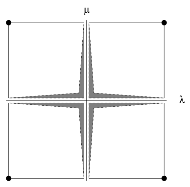
Figure 1: Subspace of A or B pairs

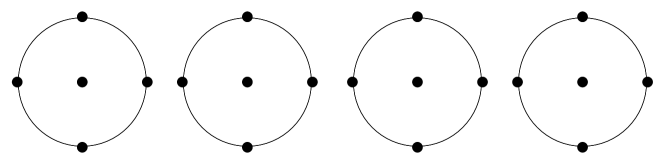
Figure 2: Subspace of B or C pairs

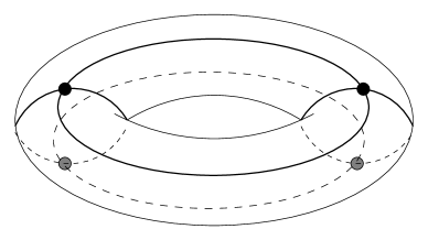
Figure 3: Subspace of B or D pairs

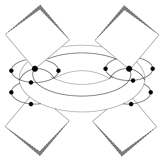
Figure 4: Overall view of the moduli space

References

• [1] Atiyah, M. F.; Bott, R.,โ€œThe Yang-Mills equations over Riemann surfaces,โ€ Philos. Trans. Roy. Soc. London Ser. A 308, 523โ€“615 (1983).
• [2] Guruprasad, K.; Huebschmann, J.; Jeffrey, L.; Weinstein, A., โ€œGroup systems, groupoids, and moduli spaces of parabolic bundles,โ€ Duke Math. J. 89, no. 2, 377โ€“412 (1997).
• [3] Goldman, William M., โ€œThe symplectic nature of fundamental groups of surfaces,โ€ Adv. Math. 54, 200โ€“225 (1984).
• [4] Hitchin, N. J., โ€œThe self-duality equations on a Riemann surface,โ€ Proc. London Math. Soc. 55 (3), 59-126 (1987)
• [5] Witten, E., โ€œ2+1 dimensional quantum gravity as an exactly solvable system,โ€ Nucl. Phys. B311, 46-78 (1988/89).
• [6] Nelson J.E.; Regge T.; Zertuche F., โ€œHomotopy Groups and $2+1$ dimensional Quantum De Sitter Gravity,โ€ Nucl. Phys. B339, 516-532 (1990); Nelson J.E.; Regge T., โ€œ2+1212+1 Quantum Gravity,โ€ Phys. Lett. B272, 213-216 (1991); Carlip S.; Nelson J.E., โ€œComparative Quantizations of 2+1 Gravity,โ€ Phys. Rev. D51, 10, 5643-5653 (1995).
• [7] Carlip, S., โ€œQuantum gravity in $2+1$ dimensions,โ€ Cambridge Monographs on Mathematical Physics, Cambridge University Press, Cambridge (1998).
• [8] Nelson, J. E.; Picken, R. F., โ€œQuantum holonomies in $(2+1)$-dimensional gravity,โ€ Phys. Lett. B 471, 367โ€“372 (2000).
• [9] Nelson, J. E.; Picken, R. F., โ€œQuantum matrix pairs,โ€ Lett. Math. Phys. 52, 277โ€“290 (2000).
• [10] Caetano, A.; Picken, R. F., โ€œAn axiomatic definition of holonomy,โ€ Int. J. Math. 5, 835โ€“848 (1994).
• [11] Barrett, J. W., โ€œHolonomy and path structures in general relativity and Yang-Mills theory,โ€ Internat. J. Theoret. Phys. 30, 1171โ€“1215 (1991).
• [12] Ezawa K., โ€œReduced Phase Space of the First Order Einstein Gravity on $\bf R\times\bf{T^{2}}$,โ€ Osaka preprint OU-HET-185 (1993),hep-th/9312151; โ€œChernโ€“Simons quantization of (2+1) anti-de Sitter gravity on a torus,โ€ Class. Quant. Grav. 12, 373-392 (1995); โ€œClassical and quantum evolutions of the de Sitter and anti-de Sitter universes in (2+1) dimensions,โ€ Phys. Rev. D49, 5211-5226 (1994), Addendum-ibid D50, 2935-2938 (1995).
• [13] de Wit, B.; Matschull, H.-J.; Nicolai, H., โ€œPhysical states in $d=3,\;N=2$ supergravity,โ€ Phys. Lett. B 318, 115โ€“121 (1993).
• [14] Louko, J.; Marolf, D. M., โ€œThe solution space of $2+1$ gravity on ${\bf R}\times T^{2}$ in Wittenโ€™s connection formulation,โ€ Class. Quant. Grav. 11, 311โ€“330 (1994).
• [15] Louko, J., โ€œWittenโ€™s $2+1$ gravity on ${R}\times$ (Klein bottle),โ€ Class. Quant. Grav. 12, 2441โ€“2467 (1995).
• [16] Falceto, F.; Gawedzki, K., โ€œChern-Simons states at genus one,โ€ Comm. Math. Phys. 159, 549โ€“579 (1994).
• [17] Ashtekar, A.; Lewandowski, J., โ€œCompleteness of Wilson loop functionals on the moduli space of ${\rm SL}(2,{C})$ and ${\rm SU}(1,1)$ connections,โ€ Class. Quant. Grav. 10, L69โ€“L74 (1993).
• [18] Mikovic, A.; Picken, R. F., โ€œSuper Chern-Simons theory and flat super connections on a torus,โ€ math-ph/0008006, to appear in Adv. Theor. Math. Phys.
Refer to caption