Quantum mechanics of layers with a finite number of point perturbations

Abstract

We study spectral and scattering properties of a spinless quantum particle confined to an infinite planar layer with hard walls containing a finite number of point perturbations. A solvable character of the model follows from the explicit form of the Hamiltonian resolvent obtained by means of Krein’s formula. We prove the existence of bound states, demonstrate their properties, and find the on-shell scattering operator. Furthermore, we analyze the situation when the system is put into a homogeneous magnetic field perpendicular to the layer; in that case the point interactions generate eigenvalues of a finite multiplicity in the gaps of the free Hamiltonian essential spectrum.

1 Nuclear Physics Institute, Academy of Sciences, 25068 Řež near a)Prague, Czechia
2 Doppler Institute, Czech Technical University, Břehová 7,
a)11519 Prague, Czechia
3 Institute of Theoretical Physics, FMP, Charles University,
a)V Holešovičkách 2, 18000 Prague, Czechia

1 Introduction

The object of our interest in this paper is a spinless quantum particle living in a layer of a fixed width $d$ with the Dirichlet boundary conditions and interacting with a finite number of point perturbations. An obvious motivation for this problem is to find a description for an electron in a semiconductor layer with impurities. However, such physical systems are in reality rather complicated objects which involve a crystal lattice with some alien atoms and an electron gas, so one has to ask first whether such a simple model can reproduce the basic features known from experiments.

It is well known that an electron in an ideally pure bulk semiconductor material can be modeled as a free particle with an effective mass $m^{*}$ which characterizes the relation between the energy and quasi-momentum at the Fermi level. Properties of the crystalline structure are thus expressed through a single material constant, which may be very different from the “bare” mass – recall that for GaAs we have $m^{*}=0.067m_{e}$.

There are two other assumptions in the “free” part of the model. The first is its one-particle character which neglects the interactions between the electrons. There are situations where the repulsion plays an important role, such as the Coulomb blockade in quantum wires. On the other hand, the one-electron model is known to work when the electron-gas density is sufficiently low. Another assumption is the neglection of spin which is also not entirely trivial; recall that spin-dependent effects in nanostructures have been studied recently – see [1] and references therein. In most situations, however, spinless electrons are a reasonable approximation.

The next question concerns the way in which we model the impurities. Using again a certain idealization, we describe them by point interactions. This method proved rather useful in the last two decades and gave rise to numerous solvable models; our aim here is to add one more class to this family. Intuitively point interactions are understood as sharply localized potentials, but it is known that a sophisticated coupling constant renormalization is required to give this concept meaning in terms of a limit of scaled potentials [2, Secs. I.1, I.5]. Mathematically such operators can be handled since they differ from the free Hamiltonian $H_{0}$ just by a change of the boundary conditions at the interaction sites. However, the counterintuitive features of three-dimensional point interactions are reflected both in the slow way in which they found their place in the theory and in the fact that the parameters appearing in these conditions cannot be interpreted as $\delta$ potential coupling constants but rather as the inverse scattering lengths corresponding to the point “obstacles” – cf. [2, Chap. I.3].

Scores of papers discussing point-interaction models in the Euclidean space, both for particles otherwise free or with a background regular potential, are summarized in the monograph [2]. Only in the last decade the attention shifted to systems with point interactions restricted to a certain region of configuration space; the reason clearly was a wide collection of new physical phenomena observed in such spatially restricted systems, mostly mesoscopic objects, but also electromagnetic waveguides, photonic crystals, etc. – see [3]. Here, too, point-interaction Hamiltonians proved as a useful tool and yielded some unexpected results such as the existence of a chaotic behaviour in systems whose classical counterparts are integrable [4].

Today there are many papers treating point interaction in restricted areas; a bibliography is given in the introduction of [5]. They typically put emphasis on the description of a specific model rather than a proper handling of the point interaction. Among few existing rigorous treatments of the problem it is the paper [5] which motivates the present study analyzing point interactions in an infinite planar strip with Dirichlet boundary conditions, together with similar systems. There are two ways in which the results can be generalized to dimension three. One is a straight Dirichlet tube in $\mathbb{R}^{3}$ with a fixed compact cross section discussed in [6]; it is a straightforward extension, apart of a different way of computing the regularized Green’s function.

In the present paper we are going to study a less trivial generalization, with point interactions situated in a flat layer with a Dirichlet boundary. The free system allows here again a separation of variables, so the free resolvent kernel and all the quantities derived from it such as eigenfunctions, etc., can be written by means of explicitly given series (in this sense models considered here are little “less solvable” than those in the full space when such quantities can be written in terms of elementary or special functions).

Although the model description is simple, it covers many different situations. For the sake of brevity we restrict ourselves in this paper to systems with a finite number of point perturbations in absence of a background potential leaving other cases to a sequel. We make an exception, however, by devoting a separate section to the case when the particle is under influence of a homogeneous magnetic field perpendicular to the layer. The spectrum of the unperturbed system is then changed completely consisting of infinitely degenerate eigenvalues which are sums of the Landau levels and the transverse eigenvalues; for “rational” combinations of parameters different Landau levels may lead to the same eigenvalue. A finite number of point perturbations then gives rise to a nontrivial discrete spectrum.

Let us describe briefly the contents. The next section is devoted to the case of a single perturbation. We start from the definition of the point-interaction Hamiltonian by means of boundary conditions coupling generalized boundary values. After that we use Krein’s formula to derive the explicit expression for the resolvent; it involves the regularized Green’s function which is given by a specific series as mentioned above – see (2.14). In Section 2.4 we use this result to analyze spectral properties of such Hamiltonians. The bound state energies are given by the implicit equation (2.18), and it is just the limits of strong and weak coupling where we are able to write the explicit expressions for the leading term of the asymptotics. In both the extreme cases the eigenvalue behavior can be easily understood: in the strong-coupling situation it goes to $-\infty$ in the same way as if there were no boundaries because the corresponding eigenfunction is strongly localized, while in the weak-coupling case the eigenvalue approaches the threshold of the essential spectrum and the wavefunction is dominated transversally by the lowest mode. We also find that the eigenvalue decreases with the distance from the layer boundary. In the last part of Section 2 we shall discuss the scattering in the presence of a perturbation. If there is a single point interaction, we can employ the symmetry of the problem with respect to rotation around the axis passing through the perturbation and perpendicular to the layer. The partial wave decomposition in the “longitudinal” coordinates shows that the only nontrivial contribution to the scattering comes from the s-wave, i.e. from states with the orbital momentum $m=0$. Within this subspace, the scattering problem is reduced to transitions between transverse modes; the final S-matrix then describes a coupling of the “open” channels, i.e. the transverse modes with the energies lower than that of the incoming spherical wave. We also derive the on-shell scattering operator which maps the incoming wave vector and transverse mode into the outgoing ones; the advantage of this approach is that it does employ the symmetry and allows for a generalization to the case with multiple perturbations.

Section 3 extends the described analysis to any finite number $N$ of point perturbations. The technique remains the same, and since the difference between the two resolvents is of rank $N$, the essential and absolutely continuous spectra are again preserved. On the other hand, the analysis of the discrete spectrum becomes more complicated. There are $n$ eigenvalues, where $1\leq n\leq N$, which are found by solving the implicit equation $\det\Lambda(z)=0$ with the $N\times N$ matrix $\Lambda$ given by (3.2). The number $n$ depends on the coupling strength. In the strong coupling limit there exist exactly $N$ eigenvalues having the same asymptotic behavior as in the one-center case. On the other hand, for weak coupling we find only one eigenvalue approaching the threshold of the essential spectrum; in this sense our system exhibits a behavior typical for all weakly coupled Schrödinger operators.

A new feature for systems with $N\geq 2$ is that they can posses eigenvalues embedded in the essential spectrum. This is possible, e.g., when the point perturbations are placed symmetrically with respect to the layer axis and have the same (sufficiently strong) coupling: the corresponding eigenfunction cannot then contain contributions from transverse modes with the energy equal or smaller than this eigenvalue. We will show that this is true for embedded eigenvalues generally: their eigenvectors have to be orthogonal to the subspace spanned by the “lower” transverse modes. For $N\geq 2$ the system exhibits no longer a rotational symmetry, hence we cannot employ the partial-wave decomposition to describe the scattering. However, the second approach mentioned above is applicable here and we can derive again the on-shell scattering operator. It is similar to that of the one-centre case differing just by replacement of a single regularized Green’s function by a sum of the elements of the matrix $\Lambda$ – see (3.31).

Section 4 deals with the situation when the layer is placed into a homogeneous magnetic field perpendicular to its boundary. The Krein’s formula is applicable but the free resolvent is substantially different from the non-magnetic case; this is reflected in the form of the essential spectrum which now consist the “sum” of the Landau levels and the transverse mode energies; it, of course, is preserved by a finite number of point perturbations. If there is a single perturbation we get exactly one eigenvalue in each spectral gap, i.e. between any two neighboring levels. In the strong and weak coupling limits it approaches the upper and lower endpoint of corresponding “free” gap, respectively. Only for the lowest gap we find a different behavior in the strong-coupling limit case; the eigenvalue goes to $-\infty$ with the same asymptotics as in the non-magnetic case. Finally we present a generalization to the case of $N$ point interactions analogous to the considerations of Section 3.

2 A Single Perturbation

2.1 The free system

Consider an infinite layer $\Sigma:=\mathbb{R}^{2}\times[0,d]$ with the coordinates denoted as $\vec{x}=(x,y)\,$, where $x=(x_{1},x_{2})\in\mathbb{R}^{2}$ and $y\in[0,d]$. We consider a single spinless nonrelativistic particle confined to $\Sigma$. Since the actual values of physical constants are not essential throughout the paper, we put $\hbar=2m=1$ and suppose that the free motion of the particle is governed by the Dirichlet Laplacian $-\Delta_{D}^{\Sigma}$.

Recall that this operator can be defined for rather general domains in $\mathbb{R}^{n}$ as the Friedrichs extension of an appropriate quadratic form [7, Sec. XIII.15]. However, since the boundary of $\Sigma$ is consists of two disjoint planes and has therefore the segment property, the operator acts simply as $H_{0}\psi=-\Delta\psi$ on the domain of all $\psi$ of the local Sobolev space $W^{2,2}(\Sigma)$ which satisfy the boundary conditions

$$\psi(x,0)=\psi(x,d)=0$$ (2.1)

for all $x\in\mathbb{R}^{2}$ – see again [7, Sec. XIII.15].

We will make use of the fact that the “longitudinal” and “transverse” variables decouple in the free system. The state Hilbert space of our problem can be then decomposed into traverse modes, $L^{2}(\Sigma)=\bigoplus_{n=1}^{\infty}L^{2}(\mathbb{R}^{2})\otimes\{\chi_{n}\}$, because the functions $\chi_{n}(y):=\sqrt{{2\over d}}\sin({\pi ny\over d})$ form an orthonormal basis in $L^{2}([0,d])$. The free Hamiltonian can be correspondingly written in the form of a direct sum,

$$H_{0}=\bigoplus_{n=1}^{\infty}\,h_{n}\otimes I_{n}\,,\quad\;h_{n}:=-{\partial^{2}\over\partial x_{1}^{2}}-{\partial^{2}\over\partial x_{2}^{2}}+\Bigl{(}{\pi n\over d}\Bigr{)}^{2}.$$ (2.2)

Since the resolvent $(H_{0}-z)^{-1}$ of the two-dimensional Laplacian is known explicitly, the above decomposition yields in turn the free resolvent kernel

$$G_{0}(x,y;x^{\prime},y^{\prime};z)={i\over 4}\sum_{n=1}^{\infty}H_{0}^{(1)}(k_{n}|x-x^{\prime}|)\,\chi_{n}(y)\,\chi_{n}(y^{\prime}),$$ (2.3)

where $k_{n}\equiv k_{n}(z):=\sqrt{z-({\pi n\over d})^{2}}\,$.

2.2 Definition of a point interaction

Our first goal is to construct a one-center perturbation supported by a point $\vec{a}:=(a,b)$ with $a\in\mathbb{R}^{2}$ and $b\in(0,d)$. This can be done in a standard way [2]. We restrict $-\Delta_{D}^{\Sigma}$ to functions which vanish in a neighborhood of $\vec{a}$; the operator obtained in this way is symmetric but not self-adjoint and we look for the perturbed one among its self-adjoint extensions. Since the restriction has deficiency indices $(1,1)$, the family of extensions is by the standard von Neumann theory [7, Sec. X.1] characterized by a single parameter.

What is equally important is that the perturbation is local, and therefore we can characterize the extensions by the usual boundary condition derived in [2, Chap. I.1] for point interactions in $\mathbb{R}^{3}$. We introduce the generalized boundary values,

$$L_{0}(\psi,\vec{a}):=\lim_{|\vec{x}-\vec{a}|\to 0}|\vec{x}-\vec{a}|\,\psi(\vec{x}),\,\quad L_{1}(\psi,\vec{a}):=\lim_{|\vec{x}-\vec{a}|\to 0}\biggl{[}\psi(\vec{x})-{L_{0}(\psi,\vec{a})\over|\vec{x}-\vec{a}|}\biggr{]}\,,$$

and require

$$L_{1}(\psi,\vec{a})-4\pi\alpha L_{0}(\psi,\vec{a})=0\,.$$ (2.4)

For a fixed $\alpha\in\mathbb{R}$ this leads to the self-adjoint operator $H(\alpha,\vec{a})$ acting as

$$(H(\alpha,\vec{a})\psi)(\vec{x})=-(\Delta\psi)(\vec{x})$$ (2.5)

for $\vec{x}\neq\vec{a}$ on the domain

$$D(H(\alpha,\vec{a})):=\Bigl{\{}\psi\,:\,-\Delta\psi\in L^{2}(\Sigma\setminus\{\vec{a}\}){\rm\;and\;(\ref{layer conditions}),\;(\ref{bc})\;are\;satisfied}\Bigr{\}}$$ (2.6)

in $L^{2}(\Sigma)$, where $-\Delta\psi$ is, of course, understood in the sense of distributions. The family of self-adjoint extension includes also case which is formally given by $\alpha=\infty$, which means $L_{0}(\psi,\vec{a})=0$. It is easy to see that the corresponding $H(\alpha,\vec{a})$ is nothing else than the free Hamiltonian $H_{0}$.

2.3 The resolvent

As usual the spectral properties of the operator $H(\alpha,\vec{a})$ can be studied using its resolvent. Since $H(\alpha,\vec{a})$ and $H_{0}$ have a common restriction with deficiency indices $(1,1)$, the kernel of the full resolvent can be obtained by means of the Krein’s formula [2, Appendix A]

$$(H(\alpha,\vec{a})-z)^{-1}(\vec{x}_{1},\vec{x}_{2})=G_{0}(\vec{x}_{1},\vec{x}_{2};z)\,+\,{G_{0}(\vec{x}_{1},\vec{a};z)\,G_{0}(\vec{a},\vec{x}_{2};z)\over\alpha-\xi(\vec{a};z)}\,,$$ (2.7)

where

$$\xi(\vec{a};z):={1\over 4\pi}\lim_{\vec{x}\to\vec{a}}\biggl{\{}{2\pi i\over d}\sum_{n=1}^{\infty}H_{0}^{(1)}(k_{n}|x-a|)\sin\Bigl{(}{\pi ny\over d}\Bigr{)}\sin\Bigl{(}{\pi nb\over d}\Bigr{)}-{1\over|x-a|}\biggr{\}}$$ (2.8)

is the regularized Green’s function; we have employed here the fact that the resolvent singularity is the same as for the kernel of $-\Delta$ in $L^{2}(\mathbb{R}^{3})$ – see [8, Sec. 13.5]. The form of the denominator in expression (2.7) follows from the boundary condition (2.4) applied to $\psi=(H(\alpha,\vec{a})-z)^{-1}\varphi$, where $\varphi$ is an arbitrary vector from $L^{2}(\Sigma)$. However, the above definition does not give a practical way to compute $\xi(\vec{a};z)$. To this end we use first $K_{0}(z)={\pi i\over 2}H_{0}^{(1)}(iz)$ and introduce $\kappa_{n}:=\sqrt{({\pi n\over d})^{2}-z}=-ik_{n}$, then we have

$$\xi(\vec{a};z)=\lim_{\varrho\to 0}\biggl{\{}{1\over\pi d}\sum_{n=1}^{\infty}K_{0}(\kappa_{n}\varrho)\sin^{2}\Bigl{(}{\pi nb\over d}\Bigr{)}\,-\,{1\over 4\pi\varrho}\biggr{\}}\,,$$ (2.9)

where $\varrho:=|x-a|$ and we have already put $y=b$. We use the asymptotic behavior $\kappa_{n}\approx{\pi n\over d}$ as $n\to\infty$ to write the identity

$$K_{0}(\kappa_{n}\varrho)=K_{0}\Bigl{(}n{\pi\varrho\over d}\Bigr{)}+\Bigl{[}K_{0}(\kappa_{n}\varrho)-K_{0}\Bigl{(}n{\pi\varrho\over d}\Bigr{)}\Bigr{]}\,.$$ (2.10)

and to divide the function $\xi$ into two parts, $\xi(\vec{a};z)=\xi_{1}+\xi_{2}$, where

$$\xi_{1} \!:=\! \lim_{\varrho\to 0}{1\over\pi d}\sum_{n=1}^{\infty}\,\Bigl{[}K_{0}(\kappa_{n}\varrho)-K_{0}\Bigl{(}{\pi n\varrho\over d}\Bigr{)}\Bigr{]}\sin^{2}\Bigl{(}{\pi nb\over d}\Bigr{)}\,,$$

$$\xi_{2} \!:=\! \lim_{\varrho\to 0}\biggl{\{}{1\over 2\pi d}\sum_{n=1}^{\infty}\,\Bigl{[}K_{0}\Bigl{(}{\pi n\varrho\over d}\Bigr{)}-K_{0}\Bigl{(}{\pi n\varrho\over d}\Bigr{)}\cos\Bigl{(}{2\pi nb\over d}\Bigr{)}\Bigr{]}-{1\over 4\pi\varrho}\biggr{\}}\,;$$

we have used $2\sin^{2}\alpha=1-\cos 2\alpha$. To deal with the first term we employ the asymptotic behavior of the Macdonald function [9, 9.6.13] which yields

$$K_{0}(\kappa_{n}\varrho)-K_{0}\Bigl{(}{\pi n\varrho\over d}\Bigr{)}=-\ln\sqrt{1-z\Bigl{(}{d\over\pi n}\Bigr{)}^{2}}\,\bigl{(}1+{\cal O}(\varrho^{2})\bigr{)}$$

as $\varrho\to 0$. It shows that the sum converges uniformly w.r.t. $\varrho$ and the limit can be interchanged with the series giving thus

$$\xi_{1}=-{1\over\pi d}\sum_{n=1}^{\infty}\,\ln\sqrt{1-z\Bigl{(}{d\over\pi n}\Bigr{)}^{2}}\,\sin^{2}\Bigl{(}{\pi nb\over d}\Bigr{)}\,.$$ (2.11)

The second part can be computed by means of the formula [10, II, 5.9.1.4.],

$$\sum_{n=1}^{\infty}\,K_{0}(nx)\cos(na)={\pi\over 2\sqrt{x^{2}+a^{2}}}+{1\over 2}\Bigl{(}\gamma+\ln{x\over 4\pi}\Bigr{)}$$

$$+\,{\pi\over 2}\sum_{n=1}^{\infty}\,\biggl{[}{1\over\sqrt{(2n\pi-a)^{2}+x^{2}}}-{1\over 2n\pi}\biggr{]}+\,{\pi\over 2}\sum_{n=1}^{\infty}\,\biggl{[}{1\over\sqrt{(2n\pi+a)^{2}+x^{2}}}-{1\over 2n\pi}\biggr{]},$$

so introducing $\beta:={b\over d},\;\mu:={\varrho\over d}$ and performing the limit $\mu\to 0$ , we get

$$\xi_{2}=\,{1\over 4\pi d}\biggl{\{}-{1\over 2\beta}-\sum_{n=1}^{\infty}{\beta^{2}\over n(n^{2}-\beta^{2})}\biggr{\}}\,.$$ (2.12)

The last sum equals using [10, I, 5.1.15.2.] expressed by means of the digamma function as $\psi(1)-{1\over 2}\bigl{(}\psi(1\!+\!\beta)+\psi(1\!-\!\beta)\bigr{)}$, and since $\psi(1)=-\gamma$, where $\gamma=0.577...$ is the Euler number, and $\psi(1-\beta)=\psi(\beta)+\pi\cot(\pi\beta),\;\psi(1+\beta)=\psi(\beta)+{1\over\beta}$, we arrive at

$$\xi_{2}=\frac{\gamma}{4\pi d}+{1\over 8\pi d}\,\Bigl{(}2\psi(\beta)+\pi\cot(\pi\beta)\Bigr{)}\,.$$ (2.13)

Putting the results together, we get the sought formula

$$\xi(\vec{a};z)=-{1\over\pi d}\sum_{n=1}^{\infty}\ln\sqrt{1\!-\!z\Bigl{(}{d\over\pi n}\Bigr{)}^{2}}\sin^{2}\Bigl{(}{\pi nb\over d}\Bigr{)}+{1\over 4\pi d}\Bigl{[}\gamma+\psi\Bigl{(}{b\over d}\Bigr{)}+{\pi\over 2}\cot\Bigl{(}{\pi b\over d}\Bigr{)}\Bigr{]}$$ (2.14)

expressing the regularized Green’s function in the form of a series. It is certainly more complicated than an expression of the corresponding quantity for the whole space in terms of elementary functions [2, Chap. I.1], but it allows us to derive the needed properties of the function $\xi$ to compute the values of $\xi(\vec{a};z)$ numerically.

Remark 2.1

Notice the scaling behavior with respect to the change of the layer thickness, i.e. the formulae relating properties of the family $\Sigma^{\sigma}=\mathbb{R}^{2}\times[0,d\sigma],\;\sigma>0$. Here the dimension of the configuration space is decisive. While for two-dimensional system the scaling amounts to logarithmic shift of the function $\xi$ as shown in [5], in three dimension the transformation is multiplicative. We find easily that the situation is the same as for straight tubes in $\mathbb{R}^{3}$ studied in [6], i.e. we have $\xi(\vec{a^{\sigma}};z\sigma^{-2})=\sigma^{-1}\xi(\vec{a};z)$, where $\vec{a^{\sigma}}:=(a\sigma,b\sigma)$. This means, in particular, that the singularities of the resolvent which we will discuss below using equation (2.18) are related as follows:

$$\epsilon^{\sigma}(\alpha^{\sigma},\vec{a^{\sigma}})=\sigma^{-2}\epsilon(\alpha,\vec{a})\,,\quad\alpha^{\sigma}:=\sigma^{-1}\alpha\,.$$ (2.15)

Without loss of generality we put therefore $d=\pi$ in the rest of this and the next section.

2.4 Spectral properties

The explicit form of the resolvent (2.7) allows us to derive information about the spectrum. Since its difference from $(H_{0}-z)^{-1}$ is a rank one operator, the essential spectrum remains by Weyl’s theorem [7, Thm. XIII.14] the same as for the free Hamiltonian $H_{0}$, i.e., we have $\sigma_{ess}(H(\alpha,\vec{a}))=[1,\infty)$. At the same time, also the absolutely continuous spectrum is preserved, $\sigma_{ac}(H(\alpha,\vec{a}))=[1,\infty)$, this time by Birman-Kuroda theorem [7, Thm. XI.9].

Next we would like to prove the absence of the singularly continuous spectrum. To this aim we have to check that the expression $(\psi,(E_{z}-E_{c})\psi)$ for all $\psi\in L^{2}(\Sigma)$ is an absolutely continuous function for $z$ from any interval $(c,t)\subset(1,\infty)$, in other words, that it can be written as an integral of a locally integrable function. Since $\sigma_{sc}$ cannot be supported by discrete points, we may choose the interval $(c,t)$ in such a way that it contains none of the points $m^{2},\;m\in\mathbb{N}$. For the spectral projection $E_{t}-E_{c}$ to the interval $(c,t)$ we employ the Stone’s formula,

$$(\psi,(E_{t}-E_{c})\psi)={1\over\pi}\,\lim_{\varepsilon\to 0_{+}}\int_{c}^{t}\left(\psi,{\rm Im\,}G(u+i\varepsilon)\psi\right)\,du\,;$$

we have used here the fact which we will establish a little later, namely that $H(\alpha,\vec{a})$ has no eigenvalues in $(1,\infty)$, and therefore the spectral projections to $(c,t)$ and $[c,t]$ are the same. The Green’s function (2.7) is analytic for $z$ with ${\rm Re\,}z\in(c,t)$ and $\pm{\rm Im\,}z\in(0,\varepsilon)$, and furthermore, its limits when $z$ approaches the real axis from above and from below exist and are continuous functions of $z$. Recall that by assumptions no thresholds are contained in $(c,t)$ and $\xi$ has nonzero imaginary part for $z\neq m^{2}$,

$${\rm Im}\,\xi(\vec{a};z)={1\over 2\pi}\,\sum\limits_{n=1}^{[\sqrt{z}]}\,\sin^{2}(nb)>0\,,$$ (2.16)

where we have used $\sqrt{z-m^{2}}=i\sqrt{m^{2}-z}$; hence the denominator of the second term in (2.7) cannot be singular. Consequently, the integrated function is bounded in $(c,t)\times[0,\varepsilon)$ and by the dominated convergence theorem the limits can be interchanged with the integral giving

$$(\psi,(E_{t}-E_{c})\psi)={1\over\pi}\,\int_{c}^{t}\left(\psi,{\rm Im\,}G(u)\psi\right)\,du.$$ (2.17)

The function under the integral is again continuous in the interval $(c,t)$, hence it is integrable and the statement is proved. If $t=t_{0}$ would be an isolated eigenvalue embedded in the continuous spectrum and $\psi$ the corresponding eigenfunction, the above relation remains valid for $t\in(t_{0}\!-\!\eta,t_{0})\cup(t_{0},t_{0}\!+\!\eta)$ with some $\eta>0$, while at the point $t_{0}$ the l.h.s. should have a jump, which is clearly impossible due to the continuity of the integrated function.

To determine the discrete spectrum, we have to find the poles of the resolvent. Recall that a perturbation which can be reduced to a self-adjoint extension of a common symmetric restriction with deficiency indices $(1,1)$ can give rise to at most one simple eigenvalue in each gap of the spectrum [11, Sec. 8.3, Cor. 1]. In our case it means one simple eigenvalue in the interval $(-\infty,1)$. In view of the relation (2.7) one can find it by solving the implicit equation

$$\xi(\vec{a};z)=\alpha$$ (2.18)

for $z\in\mathbb{R}$. The series contained in the formula (2.14) converges for all $z\in\mathbb{R}\setminus\{n^{2}:n\in\mathbb{N}\}$, because its terms decay like $n^{-2}$ as $n\to\infty$ as we can see using the Taylor expansion of $\ln(1-\zeta)$ to the first order. The remaining term $\xi_{2}$ is independent of $z$ and finite for any $b\in(0,\pi)$.

The value of $\xi(\vec{a};z)$ is real for any $z\in(-\infty,1)$. In particular, it is easy to compute

$$\xi(\vec{a};z=0)={1\over 4\pi^{2}}\left[\gamma+\psi\Big{(}{b\over\pi}\Big{)}+{\pi\over 2}\cot(b)\right]\,.$$

Differentiating $\xi(\vec{a},\cdot)$ we get

$${d\xi\over dz}={1\over 2\pi^{2}}\sum\limits_{n=1}^{\infty}\,{1\over n^{2}-z}\;\sin^{2}(nb)\,>\,0\,,$$ (2.19)

so the function is monotonously increasing for $z<1$. Moreover, it diverges at both endpoints. At the continuum threshold we have

$$\xi(\vec{a};z)=-{1\over\pi^{2}}\ln\sqrt{1-z}\,\sin^{2}(b)+{\cal O}(1)\qquad{\rm as}\qquad z\to 1-\,,$$ (2.20)

while on the opposite side we may employ a simple estimate

$$\xi(\vec{a};z)\,<\,-{1\over\pi^{2}}\ln\sqrt{1-z}\,\sin^{2}(b)+\xi_{2}\,\to\ -\infty\qquad{\rm as}\qquad z\to-\infty\,.$$

We will need a more precise asymptotics at large negative energies. Below we shall prove that

$$\xi(\vec{a};z)=-{\sqrt{-z}\over 4\pi}+{\cal O}\left(e^{-c\sqrt{-z}}\right)\qquad{\rm as}\qquad z\to-\infty$$ (2.21)

for any $c<\mathrm{dist}(\vec{a},\mathrm{bd\,}\Omega)={\pi\over 2}-\left|b-{\pi\over 2}\right|$. In other words, the leading term corresponds to the analogous function for the point-interaction Laplacian in $\mathbb{R}^{3}$ computed in [2, Chap. I.1]; it corresponds to the heuristic concept that strongly bound states are well localized, and therefore not much influenced by the presence of the boundary. Another property of $\xi(\vec{a},z)$ is its monotonicity across the halflayer,

$$\xi(\vec{a};z)>\xi(\vec{a}^{\prime};z)\qquad{\rm if}\qquad|b-\pi/2|<|b^{\prime}-\pi/2|,\;a=a^{\prime}.$$

To prove it we employ the relation (2.8) which yields

$$\xi(\vec{a};z)-\xi(\vec{a}^{\prime};z)=\lim_{|x-a|\to 0}\>{i\over 2\pi}\sum_{n=1}^{\infty}H_{0}^{(1)}(k_{n}(z)|x-a|)[\sin^{2}(nb)-\sin^{2}(nb^{\prime})]\,.$$

Since $\sin^{2}(nb)-\sin^{2}(nb^{\prime})=\sin(n(b+b^{\prime}))\sin(n(b-b^{\prime}))$ holds for $0<b^{\prime}<b\leq\pi/2$ we arrive at

$$\xi(\vec{a};z)-\xi(\vec{a}^{\prime};z)=G_{0}(a,b+b^{\prime};a,b-b^{\prime};z)\,;$$ (2.22)

the monotonicity then follows from the positivity of free resolvent kernel – cf. [7, Appendix to Sec. XIII.12]. This behavior is illustrated in Fig. 1.

Figure 1: The function $\xi(\vec{a};\cdot)$ for three different positions of the point interaction. The dash-dotted line is the leading term of the asymptotics (2.21).

This confirms the mentioned general conclusion: it follows from the stated properties of $\xi(\vec{a};\cdot)$ that the equation (2.18) has for any $\alpha\in\mathbb{R}$ a unique eigenvalue $\varepsilon(\alpha,\vec{a})$ in $(-\infty,1]$ and that the function $\varepsilon(\cdot,\vec{a})$ is monotonously increasing,

$$\varepsilon(\alpha,\vec{a})>\varepsilon(\alpha^{\prime},\vec{a})\qquad{\rm if}\qquad\alpha>\alpha^{\prime}.$$

Furthermore, $\xi(\vec{a},\cdot)$ is a real-analytic function because for a fixed $z_{1}<-1$ it is expressed on a complex neighborhood of $(-\infty,z_{1})$ through a uniformly convergent series whose terms are analytic. It follows from the implicit-function theorem that $\varepsilon(\cdot,\vec{a})$ is a $C^{\infty}$ function – see [12, Chap.XIV]. The function $\varepsilon(\cdot,\vec{a})$ is also monotonous with $b$

$$\varepsilon(\cdot,\vec{a})<\varepsilon(\cdot,\vec{a}^{\prime})\qquad{\rm if}\qquad|b-\pi/2|<|b^{\prime}-\pi/2|\,.$$ (2.23)

The behavior of the eigenvalue is shown in Fig. 2.

Figure 2: The dependence of the eigenvalues $\varepsilon(\alpha,\vec{a})$ on the parameter $\alpha$ for three positions of the point interaction.

We are also interested in the asymptotic behavior of the eigenvalue in the limits of weak and strong coupling. In the former case we have

$$\varepsilon(\alpha,\vec{a})\approx 1-\exp\left(-{2\pi^{2}\alpha\over\sin^{2}(b)}\right)\qquad{\rm as}\qquad\alpha\to\infty\,,$$ (2.24)

where the symbol $\approx$ means that for any $\epsilon>0$ and $\alpha$ large enough the eigenvalue can be squeezed between a pair of expressions from the r.h.s. in which $2\pi^{2}$ is replaced by $2\pi^{2}\pm\epsilon$. On the other hand, the strong coupling asymptotics can be proved directly. By Dirichlet bracketing [7, Sec. XIII.15] $\varepsilon(\alpha,\vec{a})$ is for $\alpha<0$ bounded from below by $-(-4\pi\alpha)^{2}$, and from above by the ground state of the Dirichlet Laplacian in a ball of radius $c$ with the point interaction in the center. The latter is easily found: writing $\varepsilon(\alpha,\vec{a})=-\kappa^{2}$ one has to solve the equation

$$(-4\pi\alpha)^{2}=\kappa^{2}(1+\sinh^{-2}\kappa c)\,.$$

It yields the sought asymptotic behavior

$$\varepsilon(\alpha,\vec{a})=-16\pi^{2}\alpha^{2}+{\cal O}\left(e^{\alpha c}\right)\qquad{\rm as}\qquad\alpha\to-\infty\,,$$ (2.25)

which justifies in view of (2.18) a posteriori the relation (2.21).

The formula (2.7) provides us with the (non-normalized) wavefunction of the bound state through the residue at the pole, $\psi(\vec{x};\alpha,\vec{a})=G_{0}(\vec{x},\vec{a};\varepsilon(\alpha,\vec{a}))$, so we have

$$\psi(\vec{x};\alpha,\vec{a})={i\over 2\pi}\sum_{n=1}^{\infty}\,H_{0}^{(1)}\left(\sqrt{\varepsilon(\alpha,\vec{a})-n^{2}}\,|x-a|\right)\sin(nb)\sin(ny).$$ (2.26)

For $\alpha\to-\infty$ we can write $H_{0}^{(1)}(u)\approx\sqrt{{2\over\pi u}}\,e^{i(u-\pi/4)}$ so we see that the wavefunction is well localized,

$$\psi(\vec{x};\alpha,\vec{a})\approx\sum_{n=1}^{\infty}\sqrt{{1\over\pi^{3}\sqrt{16\pi^{2}\alpha^{2}+n^{2}}\,|x-a|}}\>e^{-\sqrt{16\pi^{2}\alpha^{2}+n^{2}}\,|x-a|}\,\sin(nb)\sin(ny)\,;$$ (2.27)

this is illustrated in Fig. 3.

Figure 3: The unnormalized eigenfunction for $b=\pi/6$ and $\alpha=-0.1$.

On the other hand, in the limit $\alpha\to\infty$ the wavefunction for $|x-a|$ from a compact set behaves as

$$\psi(\vec{x};\alpha,\vec{a}) \!\approx\! \alpha\,{\sin y\over\sin b}\,-\,{1\over\pi^{2}}\ln|x-a|\sin b\sin y$$

$$+\,{i\over 2\pi}\,\sum_{n=2}^{\infty}\,H_{0}^{(1)}\left(\sqrt{1-n^{2}}\,|x-a|\right)\sin(nb)\sin(ny)\,.$$

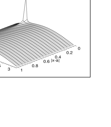
Figure 4: The unnormalized eigenfunction for $b=\pi/6$ and $\alpha=1$.

The wavefunction is dominated by the first transverse mode as Fig. 4 shows.

Let us finally return to embedded eigenvalues. We have excluded their existence away of the thresholds. If $z=m^{2}$ we use the equation (2.7) again to check that the singularities at the r.h.s. cancel. In the vicinity of $z=m^{2}$ the free resolvent kernel and the denominator $\alpha-\xi(\vec{a};z)$ behave as

$$G_{0}(\vec{x}_{1},\vec{x}_{2};z) \!=\! -\,{1\over\pi^{2}}\ln\sqrt{m^{2}-z}\,\sin(my_{1})\sin(my_{2})\left(1+{\cal O}\left(\sqrt{m^{2}-z}\right)\right),$$

$$\alpha-\xi(\vec{a};z) \!=\! \tilde{\alpha}+{1\over\pi^{2}}\ln\sqrt{m^{2}-z}\sin^{2}(mb)\,,$$

where

$$\tilde{\alpha}:=\alpha-\xi_{2}+{1\over\pi^{2}}\sum_{n\neq m}\,\ln\sqrt{1-{m^{2}\over n^{2}}}\,\sin^{2}(nb)-{1\over\pi^{2}}\ln m\sin^{2}(mb)\,.$$

Then the full-resolvent kernel asymptotically behaves as

$$\left(\tilde{\alpha}+{1\over\pi^{2}}\ln\sqrt{m^{2}-z}\,\sin^{2}(mb)\right)^{-1}{\tilde{\alpha}\over\pi^{2}}\ln\sqrt{m^{2}-z}\,\sin(my_{1})\sin(my_{2})$$

$$\phantom{AAAAAAAAAAAAAAAAAA}\times\left(1+{\cal O}\left(\sqrt{m^{2}-z}\right)\right)$$

and cannot thus have a pole-type singularity at $z=m^{2}$.

Let us summarize the results obtained so far:

Theorem 2.2

Let $H(\alpha,\vec{a})$ be defined by (2.5) and (2.6) for $d=\pi$; then
(a) $\sigma_{ess}(H(\alpha,\vec{a}))=\sigma_{ac}(H(\alpha,\vec{a}))=[1,\infty)$ and $\sigma_{sc}(H(\alpha,\vec{a}))=\emptyset$.
(b) For any $\alpha\in\mathbb{R}$ there is a single eigenvalue $\varepsilon(\alpha,\vec{a})$ in $(-\infty,1)$ which is increasing and infinitely differentiable w.r.t. $\alpha$. The corresponding eigenfunction is given by (2.26).
(c) The eigenvalue is by (2.23) strictly monotonous across the halflayer, $\varepsilon(\alpha,\vec{a})<\varepsilon(\alpha,\vec{a}^{\prime})\,$ if $\,|b-\pi/2|<|b^{\prime}-\pi/2|$.
(d) In the limit $\alpha\to\infty$ the bound state behaves according to (2.24) and (2.4). In the strong coupling case the eigenvalue asymptotics is given by (2.25) and the eigenfunction is described by (2.27).
(e) There are no eigenvalues in $[1,\infty)$.

2.5 Scattering

Since the Hamiltonian $H(\alpha,\vec{a})$ is invariant under rotations around the axis passing through the point $\vec{a}$ and perpendicular to $\Sigma$, we may simplify the treatment of stationary scattering using a partial-wave decomposition. We use the tensor-product representation

$$L^{2}(\Sigma)=L^{2}((0,\infty)\times[0,d];r\,dr\,dy)\otimes L^{2}(S^{1})\,,$$

where $S^{1}$ is the unit circle in $\mathbb{R}^{2}$ and $r:=|x|$. This can be written as

$$L^{2}(\Sigma)=\bigoplus_{m=-\infty}^{\infty}\tilde{U}^{-1}L^{2}((0,\infty)\times[0,d])\otimes\{Y_{m}\}\,,$$ (2.29)

where $\tilde{U}:\>L^{2}((0,\infty)\times[0,d];r\,dr\,dy)\to L^{2}((0,\infty)\times[0,d])$ is the unitary operator defined by $(\tilde{U}\psi)(r):=r^{1/2}\psi(r)$, the “spherical” functions $Y_{m}(\omega):=(2\pi)^{-1/2}e^{im\theta}$ with $\omega=(\cos\theta,\sin\theta)$ form a basis in $L^{2}(S^{1})$ and the symbol $\{\cdot\}$ means as above the linear envelope. Shifting the point $\vec{a}$ to the origin of the polar coordinates by $T_{a}:\>(T_{a}\phi)(x,y)=\phi(x+a,y)$, we can decompose the corresponding free Hamiltonian $H_{0}=-\Delta_{D}^{\Sigma}$ as

$$H_{0}=T_{a}^{-1}\left\{\bigoplus_{m=-\infty}^{\infty}\tilde{U}^{-1}h^{(0)}_{m}\tilde{U}\otimes I\right\}T_{a}$$ (2.30)

with the partial-wave operators

$$h_{m}^{(0)}=-{\partial^{2}\over\partial r^{2}}\,-{\partial^{2}\over\partial y^{2}}\,+{4m^{2}-1\over 4r^{2}}\,,\qquad m\in\mathbb{Z}\,.$$ (2.31)

Their domains are given in a standard way [13, Sec. 5.7]; the only non-trivial part is the radial boundary condition at the origin. As in [2, Chap. I.5] none is imposed in “higher” partial waves, $m\neq 0$, because the radial part of (2.31) is then limit-point at zero [7, Appendix to Sec. X.1]. Consequently, this part of the Hamiltonian is trivial from the point of view of the point interaction. On the other hand, for $m=0$ we introduce the generalized boundary values,

$$\ell_{0}(\phi)(y):=\lim_{r\to 0}\,\phi(r,y)\sqrt{r}\,,\quad\ell_{1}(\phi)(y):=\lim_{r\to 0}r^{-1/2}\bigl{[}\phi(r,b)-\ell_{0}(\phi)(y)r^{-1/2}\bigr{]}\,.$$ (2.32)

The s-wave component of the free Hamiltonian is specified by the condition $\ell_{0}(\phi)(y)=0$ (for any $y\in(0,d)$), while the s-wave component $h_{0}^{\alpha}$ of $H(\alpha,\vec{a})$ is given by the same differential expression (2.31) with the boundary condition at $y=b$ changed to

$$\ell_{1}(\phi)(b)-4\pi\alpha\ell_{0}(\phi)(b)=0\,.$$ (2.33)

It is also clear from this discussion that the eigenfunction of $H(\alpha,\vec{a})$ analyzed in the previous section exhibits a symmetry, $\psi(R(\varphi)\vec{x};\alpha,\vec{a})=\psi(\vec{x};\alpha,\vec{a})$, where $R(\varphi)$ is the rotation of $\Sigma$ on an angle $\varphi$ around the axis passing through the point $\vec{a}$ and perpendicular to $\Sigma$.

Let us return to the scattering problem. As in [2, Chap. I.5] the rotational symmetry means that the S-matrix part corresponding to partial waves with $m\in\mathbb{Z}\setminus\{0\}$ is trivial, i.e. the unit operator. In distinction to [2, Chap. I.5], however, the s-wave part (we denote it as $S$ again to keep the notation simple) is still in general a complicated operator because the point interaction can couple different transverse modes. Its dimension depends on the number of the “open channels”, i.e. of the transverse modes in which the particle of energy $z$ can propagate; for $d=\pi$ the latter is $[\sqrt{z}]$. Using the partial-wave operator (2.31) with $m=0$ it is easy to see that the function

$$\psi^{(0)}_{\alpha,n}(\vec{x};k) = J_{0}(k_{n}(z)r)\chi_{n}(y)$$

$$\!+\! {1\over\alpha\!-\!\xi(\vec{a};z)}\,{i\over 2\pi}\,\sum_{j=1}^{\infty}H_{0}^{(1)}(k_{j}(z)r)\sin(jb)\sin(nb)\chi_{j}(y)$$

with $r=|x-a|$ satisfies the boundary condition (2.4) and $r^{1/2}\psi^{(0)}_{\alpha,n}(\vec{x};k)$ is a generalized eigenfunction of $h_{0}^{(0)}\otimes\left(-\,{\partial^{2}\over\partial y^{2}}\right)$ with the eigenvalue $z=k^{2}$. In the limit $r\to\infty$ it behaves as

$$\psi^{(0)}_{\alpha,n}(\vec{x};k) \!\approx\! \sqrt{{2\over\pi k_{n}(z)r}}\,\cos(k_{n}(z)r-\pi/4)\chi_{n}(y)$$

$$\!+\! {1\over\alpha\!-\!\xi(\alpha;z)}\,{i\over 2\pi}\,\sum_{j=1}^{[\sqrt{z}]}\sqrt{{2\over\pi k_{j}(z)r}}\>e^{i(k_{j}(z)r-\pi/4)}\sin(nb)\sin(jb)\chi_{j}(y)\,.$$

To find the matrix elements $S_{nj}$ one has to compare this with the asymptotics of the outgoing wave in the $j$th transverse mode expressed by means of the scattering phase shift. For the wave scattered back into the incident $n$th mode we have

$$\sqrt{{2\over\pi k_{n}(z)r}}\left[\cos(k_{n}(z)r-\pi/4)+{1\over\alpha\!-\!\xi(\alpha;z)}\,{i\over 2\pi}\,e^{i(k_{m}(z)r-\pi/4)}\,\sin^{2}(nb)\right]$$

$$=\sqrt{{2\over\pi k_{n}(z)r}}\>e^{i\delta_{nn}}\cos(k_{n}(z)r-\pi/4+\delta_{nn}(k))\,,\phantom{AAAAAAAAAAAAA}$$

which yields

$$S_{nn}(k)=e^{2i\delta_{nn}(k)}=1+{i\over\pi}\,{\sin^{2}(nb)\over\alpha\!-\!\xi(\vec{a};z)}\,.$$

In a similar way scattering to the $j$th mode, $n\neq j$, requires the identification

$${1\over\alpha\!-\!\xi(\vec{a};z)}\,{i\over 2\pi}\,e^{i(k_{j}(z)r-\pi/4)}\sin(nb)\sin(jb)=e^{i\delta_{nj}(k)}\cos(k_{n}(z)r-\pi/4+\delta_{nj}(k))\,;$$

together we get

$$S_{nj}(k)=e^{2i\delta_{nj}(k)}=\delta_{nj}+{i\over\pi}\,{\sin(nb)\sin(jb)\over\alpha\!-\!\xi(\vec{a};z)}\,.$$ (2.36)

We have to check that the obtained S-matrix is unitary, i.e.

$$\sum_{j=1}^{[\sqrt{z}]}S_{nj}\bar{S}_{sj}=\delta_{ns}\,.$$ (2.37)

Using (2.36) we can write

$$\sum_{j=1}^{[\sqrt{z}]}S_{nj}\bar{S}_{sj} \!=\! \sum_{j=1}^{[\sqrt{z}]}(S_{nj}-\delta_{nj})(\bar{S}_{sj}-\delta_{js})+2{\rm Re\,}(S_{ns}-\delta_{ns})+\delta_{ns}$$

$$\!=\! {2\over\pi}\,{\sin(nb)\sin(sb)\over|\alpha\!-\!\xi(\vec{a};z)|^{2}}\left({1\over 2\pi}\,\sum_{j=1}^{[\sqrt{z}]}\sin^{2}(jb)-{\rm Im\,}\xi(\vec{a};z)\right)+\delta_{ns}\,,$$

so the desired property follows from (2.16).

The scattering problem can be also described in another way – by means of a scattering operator in $L^{2}(S^{1})\otimes L^{2}([0,d])$. Applying (2.7) to an arbitrary $\phi\in L^{2}(\Sigma)$ we see that to any $\psi\in D(H(\alpha,\vec{a}))$ and a nonreal $z$ there is $\psi_{z}\in D(H_{0})$ such that

$$\psi(\vec{x})=\psi_{z}(\vec{x})+{1\over\alpha-\xi(\vec{a},z)}\,G_{0}(\vec{x},\vec{a};z)\psi_{z}(\vec{a}).$$

If we choose, in particular, $\psi_{z}^{\varepsilon}(\vec{x})=e^{ik_{n}(z)\omega x-\varepsilon|x|^{2}}\chi_{n}(y)$ with $\omega$ a unit vector in $\mathbb{R}^{2}$, then the corresponding $\psi^{\varepsilon}(\vec{x})\in D(H(\alpha,\vec{a}))$ satisfies the equation

$$\left((H(\alpha,\vec{a})\!-\!z)\psi^{\varepsilon}\right)(\vec{x})=4\varepsilon[1\!-\!\varepsilon|x|^{2}\!+ik_{n}\omega x]\,\psi_{z}^{\varepsilon}(\vec{x})\,.$$ (2.38)

The r.h.s. converges in the $L^{2}$ sense as $z$ approaches the real line and the resulting $\psi^{\varepsilon}$ belongs to $D(H(\alpha,\vec{a}))$ for a fixed $z\in[1,\infty)$. Furthermore, the pointwise limit exists as $\varepsilon\to 0+$ and equals

$$\psi_{\alpha,n}(\vec{x};k_{n}(z)\omega)=e^{ik_{n}(z)\omega x}\chi_{n}(y)$$

$$+\,{e^{ik_{n}(z)\omega a}\over\alpha-\xi(\vec{a};z)}\,{i\over 2\pi}\,\sum_{j=1}^{\infty}H_{0}^{(1)}(k_{j}(z)|x-a|)\sin(jb)\sin(nb)\chi_{j}(y)\,.$$

The function defined by the r.h.s. is locally square integrable, solves the equation $(H(\alpha,\vec{a})\!-\!z)\psi=0$ and satisfies the appropriate boundary condition, i.e. it is a generalized eigenfunction of $H(\alpha,\vec{a})$. Let us expand it into partial waves. We know already the s-wave eigenfunction (2.5), the remaining ones are trivial, $\psi_{n}^{(m)}(\vec{x};k_{n}(z))=J_{m}(kr)\chi_{n}(y)$ if $m\neq 0$. Here again, this expression describes an eigenfunction of $h^{(0)}_{m}\otimes{\partial^{2}\over\partial y^{2}}$ in the Hilbert space (2.5), multiplying it with $r^{1/2}$ one obtains an eigenfunction in the Hilbert space (2.29). Using the known identity

$$e^{ik\omega(x-a)}=2\pi\sum_{m=-\infty}^{\infty}i^{m}J_{m}(k|x-a|)\overline{Y_{m}(\omega)}Y_{m}(\omega_{x-a})$$ (2.40)

where $Y_{m}$ are the functions introduced above and $\omega_{x-a}:={x-a\over|x-a|}$ we get

$$e^{-ik_{n}(z)\omega a}\psi_{\alpha,n}(\vec{x};k_{n}(z)\omega)=\psi^{(0)}_{\alpha,n}(\vec{x};k_{n}(z))$$

$$+2\pi\sum_{0\neq l\in\mathbb{Z}}i^{l}\psi_{n}^{(l)}(x-a,y;k_{n}(z))\overline{Y_{l}(\omega)}Y_{l}(\omega_{x-a})\,.$$

Components of the on-shell scattering amplitude $\left(f_{\alpha}(k_{n}(z),\omega_{x},\omega)\right)_{jn}$ are then given by $\lim_{|x|\to\infty,x/|x|=\omega_{x}}|x|^{{1\over 2}}e^{-ik_{j}|x|}\left[\psi_{\alpha,n}(\vec{x};k_{n}(z)\omega)-e^{ik_{n}\omega x}\chi_{n}(y)\right]$, specifically its part corresponding to the $j$th transverse mode is

$$\left(f_{\alpha}(k_{n}(z),\omega_{x},\omega)\right)_{jn}={e^{\pi i/4}\over\pi\sqrt{2\pi k_{j}(z)}}\,{\sin(jb)\sin(nb)\over\alpha-\xi(\vec{a};z)}\,e^{ik_{n}(z)\omega a-ik_{j}(z)\omega_{x}a}$$ (2.41)

and the on-shell scattering operator $S_{\alpha}(z)$ on $L^{2}(S^{1})\otimes L^{2}([0,d])$ has the form

$$S_{\alpha}(z)=I+{i\over\pi}\,\sum_{n,j=1}^{[\sqrt{z}]}{\sin(nb)\sin(jb)\over\alpha-\xi(\vec{a};z)}\,\left(e^{-ik_{n}(z)(\cdot)a}Y_{0}\chi_{n},\cdot\right)e^{-ik_{j}(z)(\cdot)a}Y_{0}\chi_{j}\,.$$ (2.42)

It follows from (2.16) that the denominator is nonzero in $[1,\infty)$. However, we have argued above that $\xi(\vec{a};\cdot)$ can be continued analytically to the complex plane where zeros exist in general. In the weak coupling case there is one resonance pole of $S_{\alpha}(z)$ close to the threshold of each higher transverse mode similarly as in the two-dimensional case [5].

3 A Finite Number of Point Interactions

3.1 Boundary conditions

Consider now a finite number $N$ of point interactions and suppose that their positions are $\vec{a}_{j}=(a_{j},b_{j})$, where $a_{j}\in\mathbb{R}^{2}$ and $b_{j}\in(0,\pi)$. For the sake of brevity we denote $\vec{a}=(\vec{a}_{1},\ldots,\vec{a}_{N})$ and $\alpha=(\alpha_{1},\ldots,\alpha_{N})$. The way to define a point interaction is the same as above; now we have $N$ independent boundary conditions

$$L_{1}(\psi,\vec{a}_{j})-4\pi\alpha_{j}L_{0}(\psi,\vec{a}_{j})=0,\qquad j=1,\ldots,N\,.$$ (3.1)

The Hamiltonian $H(\alpha,\vec{a})$ is given again by the formulae (2.5) and (2.6) with the boundary condition (2.4) replaced by (3.1) and $\vec{a}$ understood in the sense mentioned above. Any of the point interactions can be switched off when corresponding coupling constant $\alpha_{j}$ is formally put equal to infinity.

3.2 The resolvent

We again use the Krein formula to find the resolvent kernel. Since the deficiency indices of the operator obtained by restriction of the free Hamiltonian to the set of functions which vanish at the vicinity of the points $\vec{a}$ are equal to $(N,N)$, the r.h.s. is a rank $N$ operator expressed in terms of vectors from the corresponding deficiency subspaces,

$$(H(\alpha,\vec{a})-z)^{-1}(\vec{x}_{1},\vec{x}_{2})$$ (3.2)

$$=\,G_{0}(\vec{x}_{1},\vec{x}_{2};z)+\,\sum_{j,k=1}^{N}\lambda_{jk}(\alpha,\vec{a};z)\,G_{0}(\vec{x}_{1},\vec{a}_{j};z)\,G_{0}(\vec{a}_{k},\vec{x}_{2};z)\,.\phantom{AAA}$$

Applying this to an arbitrary vector of $L^{2}(\Sigma)$ we get

$$\psi(\vec{x})=\psi_{0}(\vec{x})+\sum_{j,k=1}^{N}\lambda_{jk}(\alpha,\vec{a};z)\,G_{0}(\vec{x},\vec{a}_{j};z)\,\psi_{0}(\vec{a}_{k})$$ (3.3)

with $\psi_{0}\in D(H_{0})$. The generalized boundary values are

$$L_{0}(\psi,\vec{a}_{m}) \!=\! \sum_{j,k=1}^{N}{\lambda_{jk}\over 4\pi}\,\delta_{jm}\,\psi_{0}(\vec{a}_{k})\,,$$ (3.4)

$$L_{1}(\psi,\vec{a}_{m}) \!=\! \psi_{0}(\vec{a}_{m})+\sum_{j,k=1}^{N}\lambda_{jk}\delta_{jm}\lim_{|\vec{x}-\vec{a}_{m}|\to 0}\left(G_{0}(\vec{x},\vec{a}_{j};z)-{1\over 4\pi|\vec{x}-\vec{a}_{m}|}\right)$$ (3.5)

$$+\sum_{j,k=1}^{N}\lambda_{jk}(1-\delta_{jm})G_{0}(\vec{a}_{m},\vec{a}_{j};z)\psi_{0}(\vec{a}_{k})\,.$$

The limit contained in the expression of $L_{1}(\psi,\vec{a}_{m})$ equals to $\xi(\vec{a}_{m};z)$. After substituting these boundary values into (3.1) we arrive at the conditions

$$\psi_{0}(\vec{a}_{m})+\sum_{j,k=1}^{N}\lambda_{jk}\left[\delta_{jm}(\xi(\vec{a}_{m};z)-\alpha_{m})+(1-\delta_{jm})G_{0}(\vec{a}_{m},\vec{a}_{j};z)\right]\psi_{0}(\vec{a}_{k})=0\,,$$ (3.6)

which should be satisfied for an arbitrary vector $\psi_{0}$ belonging to $D(H_{0})$, i.e. for any $N$-tuple $\left(\psi_{0}(\vec{a}_{1}),\dots,\psi_{0}(\vec{a}_{N})\right)$. This is possible only if the expressions in the square brackets are up to the sign elements of the matrix inverse to $\lambda(\alpha,\vec{a};z)$, in other words, if the coefficients are

$$\lambda(\alpha,\vec{a};z)=\Lambda(\alpha,\vec{a};z)^{-1}\,,$$ (3.7)

where

$$\Lambda_{jj} \!:=\! \alpha_{j}-\xi(\vec{a}_{j};z)$$

$$\!=\! \!\alpha_{j}+{1\over\pi^{2}}\sum_{n=1}^{\infty}\ln\sqrt{1-{z\over n^{2}}}\,\sin^{2}(nb_{j})\,-\,{1\over 4\pi^{2}}\!\left[\gamma+\psi\left({b_{j}\over\pi}\right)+{\pi\over 2}\cot(b_{j})\right]$$

$$\Lambda_{jm} \!:=\! -G_{0}(\vec{a}_{j},\vec{a}_{m};z)$$

$$\!=\! -{i\over 2\pi}\sum_{n=1}^{\infty}H_{0}^{(1)}\left(\sqrt{z-n^{2}}|a_{j}-a_{m}|\right)\,\sin(nb_{j})\sin(nb_{m})\,,\qquad j\neq m\,.$$

The Green’s function value $G_{0}(\vec{a}_{j},\vec{a}_{m};z)$ is finite for any pair of mutually different vectors $\vec{a}_{j}$ and $\vec{a}_{m}$. When the point interactions are arranged vertically, i.e. $a_{j}=a_{m}$, the expression through Hankel’s functions is useless and the corresponding nondiagonal element $\Lambda_{jm}$ can be alternatively written as

$$\Lambda_{jm} \!=\! {1\over\pi^{2}}\,\sum_{n=1}^{\infty}\,\ln\sqrt{1-{z\over n^{2}}}\,\sin(nb_{j})\sin(nb_{m})$$

$$-\xi_{2}\left({b_{j}+b_{m}\over 2}\right)+\xi_{2}\left({|b_{j}-b_{m}|\over 2}\right)\,.$$

To derive this expression we employ the argument analogous to that leading to the value of the function $\xi(\vec{a};z)$ in Section 2.3.

3.3 The discrete spectrum

Since a finite rank operator is both compact and trace class, the argument presented at the opening of Section 2.4 remains valid. In other words, a finite number of point interaction changes neither the essential nor the absolutely continuous spectrum, $\sigma_{ess}(H(\alpha,\vec{a}))=\sigma_{ac}(H(\alpha,\vec{a}))=\sigma_{ess}(H_{0})=[1,\infty)$. The singularly continuous spectrum is empty because the proof given in Sec. 2.4 can be used here again.

The discrete spectrum is determined by poles of the resolvent, which occur if the coefficient matrix $\left(\lambda_{jk}\right)^{-1}$ becomes singular. This leads to the condition

$$\det\Lambda(\alpha,\vec{a};z)=0\,.$$ (3.10)

To find the eigenfunctions we use the procedure from [2, Sec. II.1]. Suppose that $H:=H(\alpha,\vec{a})$ satisfies the equation $H\varphi=z\varphi$ for some $z\in\mathbb{R}$ and pick an arbitrary $z^{\prime}\in\varrho(H)$ . Then in accordance with (3.3) there is a function $\psi_{0}\in D(H_{0})$ which makes it possible to write

$$\varphi(\vec{x})=\psi_{0}(\vec{x})+\sum_{j=1}^{N}d_{j}G_{0}(\vec{x},\vec{a}_{j};z^{\prime})\,,$$ (3.11)

with the coefficients $d_{j}:=\sum_{k=1}^{N}(\Lambda(z^{\prime})^{-1})_{jk}\psi_{0}(\vec{a}_{k})$. We also see that

$$(H_{0}-z^{\prime})\psi_{0}=(H-z^{\prime})\varphi=(z-z^{\prime})\varphi.$$

Applying the resolvent $(H_{0}-z^{\prime})^{-1}$ to the last identity we arrive at the expression

$$\psi_{0}=(z-z^{\prime})\left[(H_{0}-z^{\prime})^{-1}\psi_{0}+\sum_{j=1}^{N}d_{j}(H_{0}-z^{\prime})^{-1}G_{0}(\cdot,\vec{a}_{j};z^{\prime})\right]\,,$$ (3.12)

which allows us to find the action of $(H_{0}-z)$ at the vector $\psi_{0}$,

$$(H_{0}-z)\psi_{0}=(H_{0}-z^{\prime})\psi_{0}-(z-z^{\prime})\psi_{0}=(z-z^{\prime})\sum_{j=1}^{N}d_{j}G_{0}(\cdot,\vec{a}_{j};z^{\prime})\,.$$ (3.13)

If $z<1$ , the resolvent $(H_{0}-z)^{-1}$ exists and may be applied to the last relation, giving by means of the first resolvent identity

$$\psi_{0}=\sum_{j=1}^{N}d_{j}[G_{0}(\cdot,\vec{a}_{j};z)-G_{0}(\cdot,\vec{a}_{j};z^{\prime})]\,.$$ (3.14)

Substituting this into (3.11) we get an expression for the eigenfunction,

$$\varphi(\vec{x})=\sum_{j=1}^{N}d_{j}G_{0}(\vec{x},\vec{a}_{j};z)\,,$$ (3.15)

where it remains to determine the coefficients. The equation (3.14) taken at the point $\vec{x}=\vec{a}_{j}$ can be rewritten using the components of matrix $\Lambda$ as

$$\psi_{0}(\vec{a}_{j})=\sum_{m=1}^{N}d_{m}\left(\Lambda(\alpha,\vec{a};z^{\prime})_{jm}-\Lambda(\alpha,\vec{a};z)_{jm}\right)\,.$$ (3.16)

We already know that $d_{m}=\sum_{k=1}^{N}(\Lambda(z^{\prime})^{-1})_{mk}\psi_{0}(\vec{a}_{k})$; taking the inverse we get $\psi_{0}(\vec{a}_{j})=\sum_{m=1}^{N}\Lambda(z^{\prime})_{jm}d_{m}$. In combination with (3.16) this yields

$$\sum_{m=1}^{N}\Lambda(z)_{jm}d_{m}=0,$$ (3.17)

i.e., $d:=(d_{1},\ldots,d_{N})$ has to be an eigenvector of the matrix $\Lambda(\alpha,\vec{a};z)$ corresponding to zero eigenvalue. The corresponding system of linear equations is solvable under the condition (3.10), and the sought eigenfunctions of $H(\alpha,\vec{a})$ are given by the formula (3.11).

It remains to check that the equation (3.10) can have a solution in $(-\infty,1)$. Let us start with the limiting situations of strong and weak coupling. We know from (2.21) how $\xi(\vec{a}_{j};z)$ behaves as $-{\sqrt{-z}\over 4\pi}$ as $z\to-\infty$. At the same time, the nondiagonal part of matrix $\Lambda$ vanishes in the limit in view of the asymptotics

$$H_{0}^{(1)}(\sqrt{z-n^{2}}|a_{j}-a_{m}|) = H_{0}^{(1)}(i\sqrt{n^{2}-z}|a_{j}-a_{m}|)$$

$$\approx \sqrt{{2\over i\pi\sqrt{n^{2}-z}\,|a_{j}-a_{m}|}}\>e^{-\sqrt{n^{2}-z}|a_{j}-a_{m}|-i\pi/4}$$

for $z\to-\infty$. This argument is not applicable if $a_{j}=a_{m}$ for $j\neq m$. Nevertheless, the nondiagonal matrix elements are up to the sign equal to Green’s function values, and thus they are bounded. In this way we get

$$\Lambda(\alpha,\vec{a};z)={\sqrt{-z}\over 4\pi}\>I+{\cal O}(1)\qquad{\rm as}\qquad z\to-\infty$$ (3.18)

with the coefficient $\alpha_{j}$ included into the error term. On the other hand,

$$\Lambda(\alpha,\vec{a};z)={1\over\pi^{2}}\ln\sqrt{1-z}\>M+{\cal O}(1)\qquad{\rm as}\qquad z\to 1-\,,$$ (3.19)

where $M:=\left(\sin b_{j}\sin b_{m}\right)_{j,m=1}^{N}$. This matrix has zero eigenvalue of multiplicity $N-1$ and the positive eigenvalue $\sum_{j=1}^{N}\sin^{2}b_{j}$ corresponding to the eigenvector $(\sin b_{1},\ldots,\sin b_{N})$. The latter is more important, because it means that one eigenvalue of $\Lambda(\alpha,\vec{a};z)$ tends to $-\infty$ as $z\to 1-$ . Furthermore, the eigenvalues of $\Lambda(\alpha,\vec{a};z)$ are continuous functions of $z$, so comparing the last claim with (3.18) we find that at least one of the eigenvalues crosses zero for some $z$, i.e. that $H(\alpha,\vec{a})$ has at least one isolated eigenvalue.

We may ask whether there some of the eigenvalues may be degenerate. For the sake of brevity we rewrite the matrix $\Lambda(\alpha,\vec{a};z)$ as

$$\Lambda(\alpha,\vec{a};z)=\delta_{jm}(\alpha_{j}-\xi_{j}(z))+(1-\delta_{jm})g_{jm}(z),$$

where $\xi_{j}(z):=\xi(\vec{a}_{j};z)$ and $g_{jm}(z):=-G_{0}(\vec{a}_{j},\vec{a}_{m};z)$. Since all $g_{jm}$ are negative, the maximum possible degeneracy is $N-1$ which means that for a pair of point interactions the discrete spectrum is always simple. Let us consider the case $N=3$. Put $z<1$, $\,\vec{a}_{1,3}=(\pm a,b_{1})$ and $\vec{a}_{2}=(0,b_{2})$. If $b_{2}\to 0$ then the value $g_{12}=g_{23}$ approaches zero being thus smaller than $g_{13}$ for $b_{2}$ small enough. On the contrary, if $b_{2}=b_{1}$ we obtain the opposite inequality; this follows from the expression (2.3) and from the monotonicity of the Macdonald function $K_{0}(u)$ with a positive argument – see [9, 9.6.24]. Hence there exists a $b_{2}\in(0,b_{1})$ such that all the non-diagonal elements of the matrix are the same, $g_{13}=g_{12}=g_{23}$. Choosing $\alpha_{j}$ which satisfy $\alpha_{j}-\xi_{j}=g_{12}$ we obtain a matrix of rank one, i.e. $z$ is an eigenvalue of multiplicity two.

3.4 Embedded eigenvalues

We have shown in the previous chapter that a single point interaction cannot produce eigenvalues embedded in the continuous spectrum. This is no longer true if $N\geq 2$ as the following example shows.

Example 3.1

Consider a pair of perturbations with the same $\alpha$ placed at $\vec{a}_{1}=(0,0,b)$ and $\vec{a}_{2}=(0,0,\pi-b)$. We can divide the eigenvalue problem into symmetric and antisymmetric parts with respect to the plane $\{(x,\pi/2)\,:\;x\in\mathbb{R}^{2}\}$. We obtain properties of the antisymmetric part by scaling the one–center problem: substituting $\sigma={1\over 2}$ into the relation (2.15) we see that the antisymmetric part has a single eigenvalue which tends to $4$ as $\alpha\to\infty$, hence it is embedded in the continuous spectrum for $\alpha$ large enough.

Thus we cannot exclude existence of embedded eigenvalues in general. We can, however, prove a weaker result. In the example the symmetry was essential, which means in particular that the eigenfunction is dominated by the second transverse mode. We will show that in general any eigenvalue $z>1$ cannot contain contributions from transverse modes with $n\leq[\sqrt{z}]$. Suppose that $H(\alpha,\vec{a})\varphi=z\varphi$ for $z>1$. We employ the relation (3.11) and take $\psi_{0}$ in the form $\psi_{0}(\vec{x})=\sum_{n=1}^{\infty}g_{n}(x)\chi_{n}(y)$, where $g_{n}\in L^{2}(\mathbb{R}^{2})$. Substituting this $\psi_{0}$ into (3.11) and using the fact that $\{\chi_{n}\}$ is an orthonormal basis in $L^{2}((0,\pi))$ we get

$$\left[-{\partial^{2}\over\partial x_{1}^{2}}-{\partial^{2}\over\partial x_{2}^{2}}-z+n^{2}\right]g_{n}(x)$$

$$=(z-z^{\prime})\sum_{j=1}^{N}d_{j}\>{i\over 4}H_{0}^{(1)}(k_{n}(z^{\prime})|x-a_{j}|)\chi_{n}(b_{j})$$

for $n=1,2,\ldots$. The Fourier–Plancherel operator transforms this into

$$\left[|p|^{2}-z+n^{2}\right]\hat{g}_{n}(p)={(z-z^{\prime})\over 2\pi}\sum_{j=1}^{N}d_{j}\>\chi_{n}(b_{j}){e^{-ipa_{j}}\over|p|^{2}-z^{\prime}+n^{2}}\,.$$ (3.20)

If $g_{n}\in L^{2}(\mathbb{R}^{2})$ then $\hat{g}_{n}$ should also belong to $L^{2}(\mathbb{R}^{2})$. It is not possible if $z>n^{2}$ and the r.h.s. of (3.20) is nonzero at $p_{n}\omega$, where $p_{n}=\sqrt{z-n^{2}}$ and $\omega$ is a unit vector in $\mathbb{R}^{2}$. Recall that the factor $(|p|^{2}-z^{\prime}+n^{2})^{-1}$ has no singularity, because $z^{\prime}\in\rho(H)$ by assumption.

To avoid the singularity of $\hat{g}_{n}$ at $|p|=p_{n}$ we have to require

$$\sum_{j=1}^{N}d_{j}\chi_{n}(b_{j})e^{-ip_{n}\omega a_{j}}=0$$ (3.21)

for an arbitrary unit vector $\omega$ from $\mathbb{R}^{2}$. If all the $a_{j}$’s are different it follows that $d_{j}\chi_{n}(b_{j})=0$ for each $j$. If some of them are the same the condition changes to $\sum_{j}d_{j}\chi_{n}(b_{j})=0$ where $j$ runs through the $a_{j}$’s which coincide. In both cases $\hat{g}_{n}$ is identically zero for $n^{2}<z$.

Consider now an arbitrary $g\in L^{2}(\mathbb{R}^{2})$ and $n^{2}<z$. Using (3.11) and (2.3) we arrive at

$$(g\chi_{n},\varphi)=(\hat{g},\hat{g}_{n})+\sum_{j=1}^{N}d_{j}\,\chi_{n}(b_{j})(g,{i\over 4}H_{0}^{(1)}(k_{n}(z^{\prime})|x-a_{j}|))\,.$$ (3.22)

The first scalar product is equal to zero because $\hat{g}_{n}$ is zero. If all the $a_{j}$’s are different then $d_{j}\chi_{n}(b_{j})=0$ for all $j$ and the whole r.h.s. is equal to zero. If some $a_{j}$’s are the same, the condition $\sum_{j=1}^{N}d_{j}\chi_{n}(b_{j})=0$ leads to $(g\chi_{n},\varphi)=0$ again. The conclusion holds true for all $n=1,\ldots,[\sqrt{z}]$ what we have set out to prove.

3.5 The limits of strong and weak coupling

Of the two extreme situations, consider first the strong coupling. One can write the matrix $\Lambda(\alpha,\vec{a};z)$ in the form

$$\Lambda(z)=\left(\left(\alpha_{j}+{\sqrt{-z}\over 4\pi}\right)\delta_{jk}\right)\left[I+\left(\left(\alpha_{j}+{\sqrt{-z}\over 4\pi}\right)\delta_{jk}\right)^{-1}\tilde{\Lambda}(z)\right],$$

where $\tilde{\Lambda}(z)$ is the remainder matrix, which is independent of $\alpha_{j}$ and has a bounded norm as $z\to-\infty$. For an arbitrary finite interval $J\subset(-\infty,1)$ we can always choose $\alpha_{j}$’s large enough negative that no eigenvalues are contained in $J$ and the two matrices in the above product are regular in $J$. It means that the roots of equation (2.18) come from the region where $\Lambda(z)$ is dominated by its diagonal part. Then there are exactly N eigenvalues (including a possible degeneracy), which behave asymptotically as

$$\varepsilon_{j}(\alpha,\vec{a})\approx-16\pi^{2}\alpha_{j}^{2}\qquad{\rm as}\qquad\max_{1\leq j\leq N}\alpha_{j}\to-\infty.$$ (3.23)

As we expect the eigenfunctions in the strong limit are strongly localized and only slightly influenced by the other perturbations. The eigenfunction localized at $\vec{a}_{j}$ has the same form as in the Section 2.4 where we put $\vec{a}=\vec{a}_{j}$.

Consider now on the contrary that all the point interactions are weak, i.e. that all the $\alpha_{j}$’s are large positive. Denoting $A:={\rm diag}(\alpha_{1},\ldots,\alpha_{N})$ we can write

$$\Lambda(z)=A+{1\over\pi^{2}}\ln\sqrt{1-z}\,M\,+\,\tilde{\Lambda}(z)$$ (3.24)

where $\tilde{\Lambda}(z)$ is a remainder matrix, which is again independent of $\alpha$ with its norm bounded, $\|\tilde{\Lambda}(z)\|\leq C_{\vec{a}}$ for $z\in(z_{0},1)$. In Section 3.3 we found that $\Lambda(z)$ was asymptotically a rank–one operator on $\mathbb{C}^{N}$. Hence only one isolated eigenvalue of $H(\alpha,\vec{a})$ exists in this asymptotic situation.

To find the leading term of the asymptotic expansion, we have to solve the spectral problem for matrix $M-\eta A-\eta\tilde{\Lambda}(z)$, where $\eta:=-2\pi^{2}(\ln(1\!-\!z))^{-1}$. The largest eigenvalue of this matrix satisfies $\mu_{N}(\eta)\geq\mu_{N}(0)-(C_{\vec{a}}\!+\!\alpha_{+})\eta$, where $\alpha_{+}:=\max\alpha_{j}$, while for $j=1,\dots,N\!-\!1$ we have $\mu_{j}(\eta)\leq(C_{\vec{a}}\!-\!\alpha_{-})\eta$, where $\alpha_{-}:=\min\alpha_{j}$. Since $\mu_{N}(0)>0$ we see that for $\alpha_{-}$ large enough the condition has just one solution for $\eta>0$. One can check directly that without $\tilde{\Lambda}(z)$ the condition is satisfied for $\eta=\sum_{j}\alpha_{j}^{-1}\sin^{2}b_{j}$. Thus $\eta={\cal O}(\alpha_{-}^{-1})$ and the eigenvalue expansion follows. Hence the bound-state energy in weak-coupling case behaves as

$$\varepsilon(\alpha,\vec{a})\approx 1-\exp\left\{-2\pi^{2}\left(\sum_{j=1}^{N}{\sin^{2}b_{j}\over\alpha_{j}}\right)^{-1}\right\}$$ (3.25)

as $\min_{1\leq j\leq N}\alpha_{j}\to\infty$. Since the eigenvector of matrix $M$ corresponding to the nonzero eigenvalue is $(\sin b_{1},\ldots,\sin b_{N})$, the asymptotic expression of the eigenfunction for $\vec{x}$ from a restricted part of $\Sigma$ is

$$\varphi(\vec{x})\approx\sin y\left({\sum_{j=1}^{N}\sin^{2}b_{j}\over\sum_{j=1}^{N}{\sin^{2}b_{j}\over\alpha_{j}}}\,-\,{1\over\pi^{2}}\sum_{j=1}^{N}\sin^{2}b_{j}\,\ln|x-a_{j}|\right)$$ (3.26)

$$+\,{1\over\pi^{2}}\,\sum_{n=2}^{\infty}\sin(ny)\,\sum_{j=1}^{N}\sin b_{j}\,\sin(nb_{j})\,K_{0}\left(\sqrt{n^{2}-1}|x-a_{j}|\right)\,.\phantom{AAA}$$

Let us summarize the spectral properties of our Hamiltonian in the $N$-center case derived in the previous three paragraphs.

Theorem 3.2

Let $H(\alpha,\vec{a})$ be defined by (2.5) and (2.6) for $d=\pi$, where $\vec{a}=(\vec{a}_{1},\ldots,\vec{a}_{N})$ and $\alpha=(\alpha_{1},\ldots,\alpha_{N})$ and the boundary condition (2.4) is replaced by (3.1); then
(a) $\sigma_{ess}(H(\alpha,\vec{a}))=\sigma_{ac}(H(\alpha,\vec{a}))=[1,\infty)$ and $\sigma_{sc}(H(\alpha,\vec{a}))=\emptyset$.
(b) For any $\alpha\in\mathbb{R}^{N}$ there is at least one eigenvalue $\varepsilon(\alpha,\vec{a})$ in $(-\infty,1)$. The maximum number of eigenvalues is $N$ with the multiplicity taken into account; the maximum multiplicity is $N-1$. The corresponding eigenfunction is given by (3.15), where the coefficients $d_{m},\;m=1,\ldots,N$, are components of a vector solving the equation $\Lambda d=0$ with the matrix $\Lambda$ given by (3.2).
(c) In the limit $\min_{1\leq j\leq N}\alpha_{j}\to\infty$ the bound state wave function behaves according to (3.25) and (3.26). On the other hand, in the strong coupling case there are exactly $N$ eigenvalues whose asymptotics is given by (3.23); the corresponding eigenfunctions are strongly localized around the points $\vec{x}=\vec{a}_{j}$ and given by (2.27) with $\vec{a}=\vec{a}_{j}$ and $\alpha=\alpha_{j}$.
(d) If an eigenvalue $z\in[1,\infty)$ exists, the corresponding eigenvector is orthogonal to the subspace $\bigoplus_{n=1}^{[\sqrt{z}]}L^{2}(\mathbb{R}^{2})\otimes\{\chi_{n}\}$.

3.6 Scattering

Comparing to the one-center case, the Hamiltonian $H(\alpha,\vec{a})$ with a finite number of perturbations loses in general the invariance with respect to rotations around an axis perpendicular to $\Sigma$. Hence we cannot employ here the partial wave decomposition and we turn directly to the “closed form” of the on–shell scattering amplitude and on–shell scattering operator. By (3.3), to any $\psi\in D(H(\vec{a},\alpha))$ and a nonreal $z$ there exists $\psi_{z}\in D(H_{0})$ such that

$$\psi(\vec{x})=\psi_{z}(\vec{x})+\sum_{j,k=1}^{N}\lambda_{jk}(\alpha,\vec{a};z)\,G_{0}(\vec{x},\vec{a}_{j};z)\,\psi_{z}(\vec{a}_{k}).$$ (3.27)

We take again $\psi_{0}^{\varepsilon}(\vec{x})=e^{ik_{n}(z)\omega x-\varepsilon|x|^{2}}\chi_{n}(y)$ for $\psi_{z}$, where $\omega$ is a unit vector in $\mathbb{R}^{2}$. Denoting the l.h.s. of (3.27) as $\psi^{\varepsilon}$ we have $\psi^{\varepsilon}\in D(H(\alpha,\vec{a}))$ and

$$\left((H(\alpha,\vec{a})\!-\!z)\psi^{\varepsilon}\right)(\vec{x})=4\varepsilon[1\!-\!\varepsilon|x|^{2}\!+ik_{n}\omega x]\,\psi_{z}^{\varepsilon}(\vec{x})\,.$$ (3.28)

The r.h.s. converges in $L^{2}(\mathbb{R}^{2})$ as $z$ approaches the real line and the $\psi^{\varepsilon}$ belongs to $D(H(\alpha,\vec{a}))$. The pointwise limit $\varepsilon\to 0+$ exists and equals

$$\psi_{\alpha,n}(\vec{x};k_{n}(z)\omega)=e^{ik_{n}(z)\omega x}\chi_{n}(y)+\sum_{j,k=1}^{N}\lambda_{jk}(\alpha,\vec{a};z)\,G_{0}(\vec{x},\vec{a}_{j};z)\,e^{ik_{n}(z)\omega a_{k}}\chi_{n}(b_{k}).$$ (3.29)

The limiting function is locally square integrable and it thus is a generalized eigenfunction of $H(\alpha,\vec{a})$.

The components $\left(f_{\alpha}(k_{n}(z),\omega_{x},\omega)\right)_{mn}$ of the on–shell scattering amplitude are then given by the part of the following expression corresponding to the outgoing $m$th transverse mode,

$$\lim_{|x|\to\infty,x/|x|=\omega_{x}}|x|^{1/2}e^{-ik_{m}|x|}\left[\psi_{\alpha,n}(\vec{x};k_{n}(z)\omega)-e^{ik_{n}\omega x}\chi_{n}(y)\right]\,.$$

It yields

$$\left(f_{\alpha}(k_{n}(z),\omega_{x},\omega)\right)_{mn} = {e^{i\pi/4}\over\pi\sqrt{2\pi k_{m}(z)}}\,\sum_{j,k=1}^{N}e^{-ik_{m}(z)\omega_{x}a_{j}}\,\lambda_{jk}(\alpha,\vec{a};z)\,e^{ik_{n}(z)\omega a_{k}}$$ (3.30)

$$\times\>\sin(mb_{j})\sin(nb_{k})\,,$$

and the on-shell scattering operator $S_{\alpha}(z)$ on $L^{2}(S^{1})\otimes L^{2}([0,d])$ is

$$S_{\alpha}(z) = I+{i\over 2\pi^{2}}\,\sum_{k,j=1}^{N}\sum_{m,n=1}^{[\sqrt{z}]}\sin(mb_{j})\sin(nb_{k})\,\lambda_{jk}(\alpha,\vec{a};z)\,\left(e^{-ik_{n}(z)(\cdot)a_{k}}\chi_{n},\cdot\right)$$ (3.31)

$$\times\>e^{-ik_{m}(z)(\cdot)a_{j}}\chi_{m}\,.$$

As in the one-center case, resonances are determined by the poles in the meromorphic continuation of the matrix-valued function $(\lambda_{jk}(\alpha,\vec{a};\cdot))$.

4 A Layer in Magnetic Field

4.1 The free Hamiltonian

In this section, the layer $\Sigma=\mathbb{R}^{2}\times(0,d)$ is placed into a homogeneous magnetic field $\vec{B}=(0,0,B)$. As usual the vector potential generating this field can be chosen in different ways, e.g. we can employ the symmetric gauge, $\vec{A}={1\over 2}(-Bx_{2},Bx_{1},0)$. We again use the decomposition into transverse modes,

$$H_{0}^{B} = \bigoplus_{n=1}^{\infty}h_{n}^{B}\otimes I_{n},$$ (4.1)

$$h_{n}^{B} = \left(-i{\partial\over\partial x_{1}}+{1\over 2}Bx_{2}\right)^{2}+\left(-i{\partial\over\partial x_{2}}-{1\over 2}Bx_{1}\right)^{2}+\left({\pi n\over d}\right)^{2}.$$

The first two terms at the r.h.s. denoted as $h^{B}$ describe a two-dimensional particle in the perpendicular homogeneous field. The resolvent kernel of such an operator is well known [14]:

$$\left(h^{B}-z\right)^{-1}(x,x^{\prime}) \!=\! {1\over 4\pi}\,\exp\left({iB\over 2}\,(-x_{1}x^{\prime}_{2}+x_{2}x^{\prime}_{1})-{|B|\over 4}\,|x-x^{\prime}|^{2}\right)$$

$$\times\>\Gamma\left({|B|-z\over 2|B|}\right)U\left({|B|-z\over 2|B|},1;{|B|\over 2}\,|x-x^{\prime}|^{2}\right)\,,$$

where $U$ is the irregular confluent hypergeometric function [9, 13.1.33]. For the sake of brevity we denote the exponential term in the above formula as $\Phi^{B}(x,x^{\prime})$. The decomposition (4.1) then yields the sought resolvent kernel

$$G_{0}^{B}(\vec{x},\vec{x}^{\prime};z) \!\equiv\! \left(H_{0}^{B}-z\right)^{-1}(x,y;x^{\prime},y^{\prime})$$ (4.2)

$$\!=\! {1\over 2\pi d}\,\exp\left({iB\over 2}\,(-x_{1}x^{\prime}_{2}+x_{2}x^{\prime}_{1})-{|B|\over 4}\,|x-x^{\prime}|^{2}\right)$$

$$\times \sum_{n=1}^{\infty}\>\Gamma\left({|B|-k_{n}^{2}(z)\over 2|B|}\right)U\left({|B|-k_{n}^{2}(z)\over 2|B|},1;{|B|\over 2}\,|x-x^{\prime}|^{2}\right)$$

$$\times \sin\left({n\pi y\over d}\right)\sin\left({n\pi y^{\prime}\over d}\right).$$

4.2 The perturbed resolvent

As in the non-magnetic case we start from a single point interaction located at the point $\vec{a}\in\Sigma$ and modify to the present situation the argument of Sec. 2.3. We employ the fact that locally the magnetic field means a regular perturbation of the Schrödinger equation; motivated by this we define the one-center Hamiltonian in the same way as in Chap. 2: it acts as free

$$(H^{B}(\alpha,\vec{a})\psi)(\vec{x})$$

$$=\left(\left[\left(-i{\partial\over\partial x_{1}}+{1\over 2}Bx_{2}\right)^{2}+\left(-i{\partial\over\partial x_{2}}-{1\over 2}Bx_{1}\right)^{2}-{\partial^{2}\over\partial y^{2}}\right]\psi\right)(\vec{x})$$

for $\vec{x}\neq\vec{a}$ with the domain changed to

$$D(H^{B}(\alpha,\vec{a})) \!=\! \{\,\psi\in L^{2}(\Sigma\setminus\{\vec{a}\}):\;H^{B}(\alpha,\vec{a})\psi\in L^{2}(\Sigma\setminus\{\vec{a}\}),$$

$$\psi(x,0)=\psi(x,d)=0,\;L_{1}(\psi,\vec{a})-4\pi\alpha L_{0}(\psi,\vec{a})=0\,\}\,,$$

where $L_{0}$ and $L_{1}$ in the last relation are again the generalized boundary values from [2, Chap. I.1].

Remark 4.1

To justify such a definition we have to check that the resolvent kernel (4.2) has the same singularity as the non-magnetic expression (2.3) for $\vec{x}^{\prime}\to\vec{x}$. We have $G^{B}_{0}(\vec{x},\vec{x}^{\prime};z)\approx c|\vec{x}^{\prime}-\vec{x}|^{-1}$ by [15, Thm. III.5.1] with a non-zero $c$ independent of $z$. To check that the constant has the needed value it is sufficient to find operators $H_{-}$ and $H_{\beta}$ with $\beta$ from some interval $(\beta_{0},1)$ whose resolvent kernels are $\sim(4\pi)^{-1}|\vec{x}^{\prime}-\vec{x}|$ around the singularity and which satisfy the inequalities

$$H_{-}\leq H_{0}^{B}\leq\beta^{-1}H_{\beta}\,,$$ (4.5)

since the last named property implies easily

$$(H_{-}-z)^{-1}\geq(H_{0}^{B}-z)^{-1}\geq\beta(H_{\beta}-\beta z)^{-1}$$

for a fixed $z<0$ and $c=(4\pi)^{-1}$ follows by contradiction. For the lower bound we choose the projection to the layer of the magnetic Schrödinger operator $(-i\vec{\nabla}-\vec{A})^{2}$ in $L^{2}(\mathbb{R}^{3})$ obtained by removing the Dirichlet boundaries of $\Sigma$, because the latter is of the form $h_{B}\otimes I+I\otimes(-\partial_{y}^{2})$ and we may apply the bracketing argument [7, Sec. XIII.15] to the non-magnetic part in the $y$-direction. Its kernel is known [16, 17] to be

$$\widetilde{G}_{0}^{B}(\vec{x},\vec{x}^{\prime};z) = {1\over 4\pi}\left({|B|\over 2}\right)^{1/2}\Phi^{B}(x,x^{\prime})$$

$$\times\sum_{l=0}^{\infty}{\exp\left[-(|B|(2l+1)-z)^{1/2}|y\!-\!y^{\prime}|\right]\over\left(l+{1\over 2}-{z\over 2|B|}\right)^{1/2}}\,L_{l}\left({B\over 2}|x\!-\!x^{\prime}|^{2}\right),$$

where the factor $\Phi^{B}$ is the same as in the relation (4.2) and $L_{l}$ are the Laguerre polynomials. We want to prove that $|\vec{x}-\vec{x}^{\prime}|\widetilde{G}_{0}^{B}(\vec{x},\vec{x}^{\prime};z)$ tends to $(4\pi)^{-1}$ in the limit $|\vec{x}-\vec{x}^{\prime}|\to 0$. Putting $|x-x^{\prime}|=0$, we can neglect the Laguerre polynomials and the factor $\Phi^{B}$; it remains to compute the simplified sum. For a given $z$ there exists an integer number $l_{0}$ such that $|B|(2l_{0}-1)-z>0$. Then one could split the series into two parts: the finite sum over $l=0,\ldots,l_{0}-1$ which is irrelevant for the singularity and the truncated series with $l=l_{0},\ldots\>$. The latter can be estimated as follows,

$$I_{-}\leq{|B|\over 4\pi}\sum_{l=l_{0}}^{\infty}{\exp\left[-(|B|(2l+1)-z)^{1/2}\varrho\right]\over\left(|B|(2l+1)-z\right)^{1/2}}\leq I_{+},$$ (4.7)

where

$$I_{\pm}:={|B|\over 4\pi}\int_{l_{0}}^{\infty}{\exp\left[-(|B|(2l\mp 1)-z)^{1/2}\varrho\right]\over(|B|(2l\mp 1)-z)^{1/2}}\,dl\,=\,{1\over 4\pi\varrho}\>e^{-(|B|(2l_{0}\mp 1)-z)^{1/2}\varrho}\,.$$

Hence the resolvent $\widetilde{G}_{0}^{B}$ has the needed singularity.

In he opposite direction we add a Dirichlet boundary at $|x|=R$ cutting thus a finite cylinder of $\Sigma$. It is clearly sufficient to find a bound of the type (4.5) for the “planar” part of the operator and this task is further reduced to finding bounds for its partial-wave components,

$$\tilde{h}_{m}^{B}=-\,{\partial^{2}\over\partial r^{2}}\,-\,{1\over r}\,{\partial\over\partial r}\,+\,\left({m\over r}-{Br\over 2}\right)^{2}$$ (4.8)

on $L^{2}(0,R)$ with the boundary condition $\lim_{r\to 0}\phi(r)(r^{1/2}\ln r)^{-1}=0$ at the origin [2, Sec. I.5] and Dirichlet at $r=R$. A comparison of the potential terms shows that $\tilde{h}_{m}^{B}\leq\beta^{-1}\tilde{h}_{m}^{0}$ holds if $R<\left({2\over|B|}(\beta^{-1/2}\!-1)\right)^{1/2}$, so one can choose for $H_{\beta}$ the non-magnetic Dirichlet Laplacian in the cylinder of an arbitrarily small radius. This operator has again the resolvent kernel with the needed singularity [8]. Notice finally that alternative ways to prove this result can be found in [18] or derived by techniques from the classical theory of partial differential equations [19, Thm. 20.6].

Remark 4.2

The previous remark still does not answer the question about the Green’s function singularity fully. To explain why it is the case, recall that the requirement of symmetry of the magnetic Hamiltonian yields for any functions $\psi_{1},\,\psi_{2}$ from the domain by means of the Gauss theorem the condition [18]

$$\lim_{r\to 0}\int_{S_{\vec{a}}}\left(-\bar{\psi}_{1}{\partial\psi_{2}\over\partial r}+\psi_{2}{\partial\bar{\psi}_{1}\over\partial r}+2i\bar{\psi}_{1}\psi_{2}{\vec{A}\vec{r}\over r}\right)dS\,=\,0\,,$$

where $\vec{r}=\vec{x}-\vec{a}$, $r=|\vec{r}|$ and the integral is taken over the surface of the sphere $S_{\vec{a}}$ with center at $\vec{a}$ and radius $r$. It is satisfied if the functions have the following asymptotic behaviour in the vicinity of the point interaction:

$$\psi(\vec{x})=c_{0}{1+\vec{A}(\vec{a})(\vec{x}-\vec{a})\over|\vec{x}-\vec{a}|}+c_{1}+{\cal O}(|\vec{x}-\vec{a}|).$$ (4.9)

This motivates us to change the generalized boundary value $L_{1}$ to

$$L_{1}(\psi,\vec{a})\,=\,\lim_{|\vec{x}-\vec{a}|\to 0}\left[\psi(\vec{x})-L_{0}(\psi,\vec{a})\,{1+i\vec{A}(\vec{a})(\vec{x}-\vec{a})\over|\vec{x}-\vec{a}|}\right].$$ (4.10)

This suggests to use for $\xi(B,\vec{a};z)$ the following limit

$$\xi(B,\vec{a};z)\,=\,\lim_{\vec{x}\to\vec{a}}\left[G_{0}^{B}(\vec{x},\vec{a};z)-{1+i\vec{A}(\vec{a})(\vec{x}-\vec{a})\over 4\pi|\vec{x}-\vec{a}|}\right],$$ (4.11)

which has the disadvantage that it is direction-dependent and can be altered by a gauge change.

However, it is possible to employ the function $\xi(B,\vec{a};z)$ defined by means of the pole singularity alone. By (4.2) the Green function $G_{0}^{B}(\vec{x},\vec{a};z)$ has the form $\exp(i\vec{A}(\vec{a})(\vec{x}-\vec{a}))F(|\vec{x}-\vec{a}|;z)$ in the symmetric gauge. In Remark 4.1 we have shown that $F(|\vec{x}-\vec{a}|;z)$ has the following asymptotic behaviour for small $|\vec{x}-\vec{a}|$,

$$F(|\vec{x}-\vec{a}|;z)={1\over 4\pi|\vec{x}-\vec{a}|}+c(z)+{\cal O}(|\vec{x}-\vec{a}|),$$

where $c(z):=\lim_{\varrho\to 0}\left[F(\varrho;z)-{1\over 4\pi\varrho}\right]$. The function $c$ defined in this way can be understood as $\xi(B,\vec{a};z)$ obtained for the Green’s function without the exponential factor; the corresponding generalized boundary value $L_{1}$ does not contain the extra part $\vec{A}(\vec{a})(\vec{x}-\vec{a})$. In the respective asymptotic formula for complete Green’s function one has to multiply the last expression by two first terms of Taylor series of the exponential factor,

$$G_{0}^{B}(\vec{x},\vec{a};z)={1+i\vec{A}(\vec{a})(\vec{x}-\vec{a})\over 4\pi|\vec{x}-\vec{a}|}+c(z)+{\cal O}(|\vec{x}-\vec{a}|).$$

Using now the modified boundary value $L_{1}$ we find that $\xi(B,\vec{a};z)=c(z)$. This justifies the choice of the generalized boundary values made in the beginning of this section; one has to keep in mind to ignore the exponential term $\Phi^{B}(x,a)$ when computing $\xi(B,\vec{a};z)$. This argument remains also valid for a finite number of point interactions, hence the functions $\xi(B,\vec{a}_{j};z)$ for $j=1,\ldots,N$ contained in matrix $\Lambda(B,\alpha,\vec{a};z)$ in Section 4.4 below are computed in the way described here.

After this digression we can return to evaluation of the Green’s function of the operator $H^{B}(\alpha,\vec{a})$. By construction it is given by the Krein’s formula,

$$G^{B}(\vec{x},\vec{x}^{\prime};z)=G^{B}_{0}(\vec{x},\vec{x}^{\prime};z)\,+\,{G^{B}_{0}(\vec{x},\vec{a};z)G^{B}_{0}(\vec{a},\vec{x}^{\prime};z)\over\alpha-\xi(B,\vec{a};z)}\,,$$ (4.12)

where the regularized Green’s function $\xi(B,\vec{a};\cdot)$ is, as we have explained in the above remarks, now given by

$$\xi(B,\vec{a};z)=\lim_{|\vec{x}-\vec{a}|\to 0}\left[G^{B}_{0}(\vec{x},\vec{a};z)-{1\over 4\pi|\vec{x}-\vec{a}|}\right]$$ (4.13)

$$= \lim_{\varrho\to 0}\Biggl{[}{1\over 2\pi d}\sum_{n=1}^{\infty}\Gamma\left({|B|-k_{n}^{2}(z)\over 2|B|}\right)U\left({|B|-k_{n}^{2}(z)\over 2|B|},1;{|B|\over 2}\varrho^{2}\right)$$

$$\qquad\qquad\qquad\times\>\sin^{2}\left({n\pi b\over d}\right)-{1\over 4\pi\varrho}\,\Biggr{]}\,.$$

One can check directly the consistency requirement

$$\lim_{B\to 0}G^{B}(\vec{x},\vec{x}^{\prime};z)=G(\vec{x},\vec{x}^{\prime};z)$$ (4.14)

for fixed $\alpha,\vec{a}$ and $\vec{x}\neq\vec{x}^{\prime}$, where $G(\cdot,\cdot;z)$ is the non-magnetic Green’s function of Sec. 2.3. It follows easily from a known relation [9, 13.3.3] for the confluent hypergeometric function,

$$\lim_{u\to\infty}\Gamma(u)U\left(u,1,{s\over u}\right)=2K_{0}\left(2\sqrt{s}\right)\,.$$

To make use of the Green’s function, we have to evaluate the r.h.s. of (4.13). We employ again the same trick and split a part of the series which can be summed explicitly for a general $\varrho$ while in the remaining series the limit $\varrho\to 0$ can be interchanged with the sum. Since $U(u,1;\cdot)$ and $K_{0}(\cdot)$ have both a logarithmic singularity at zero, we modify the Ansatz of Sec. 2.3 writing $\xi(B,\vec{a};z)=\xi_{1}+\xi_{2}$ with

$$\xi_{1} := \lim_{\varrho\to 0}\,{1\over 2\pi d}\sum_{n=1}^{\infty}\left[\Gamma\left({|B|-k_{n}^{2}(z)\over 2|B|}\right)U\left({|B|-k_{n}^{2}(z)\over 2|B|},1;{|B|\over 2}\varrho^{2}\right)\right.$$

$$\left.-\,2K_{0}\left(\varrho{\pi n\over d}\right)\right]\sin^{2}\left({n\pi b\over d}\right),$$

$$\xi_{2} := \lim_{\varrho\to 0}\left[{1\over 2\pi d}\sum_{n=1}^{\infty}2K_{0}\left(\varrho{\pi n\over d}\right)\sin^{2}\left({n\pi b\over d}\right)-{1\over 4\pi\varrho}\right].$$

The function $\xi_{2}$ is evaluated as above: in analogy with (2.13) we have

$$\xi_{2}={\gamma\over 4\pi d}+{1\over 8\pi d}\left(2\psi\left({b\over d}\right)+\pi\cot\left({\pi b\over d}\right)\right)\,.$$ (4.15)

As for the first part $\xi_{1}$, we employ the small $\varrho$ asymptotics for the confluent hypergeometric and Macdonald functions,

$$U(u,1;s) \!=\! -\,{1\over\Gamma(u)}\left[\,\ln s+\psi(u)-2\psi(1)\,\right]+{\cal O}(|s\ln s|)\qquad{\rm as}\qquad s\to 0\,,$$

$$K_{0}(s) \!=\! -\left[\,\ln{s\over 2}-\psi(1)\,\right]+{\cal O}(s^{2})\qquad{\rm as}\qquad s\to 0$$

(see [20, 6.7.13] and [9, 9.6.13]). Putting them together we see that the summand behaves for small $\varrho$ as

$$\ln\left((\pi n)^{2}\over 2|B|d^{2}\right)-\psi\left({|B|-z+\left({\pi n\over d}\right)^{2}\over 2|B|}\right)+{\cal O}\left(|\varrho^{2}\ln\varrho|\right).$$

For large $n$ the digamma function $\psi(s)=\ln(s)-2/s+{\cal O}(s^{-2})$, so the above expression can be written for large $n$ as

$$-\ln\left(1+(|B|-z)\left({d\over\pi n}\right)^{2}\right)+{1\over 2}{2|B|\over|B|-z+\left({\pi n\over d}\right)^{2}}+{\cal O}(n^{-4})$$

$$\phantom{AAA}=z\left({d\over\pi n}\right)^{2}+{\cal O}(n^{-4})\,.\phantom{AAAAAAAA}$$

Hence the series in the definition of $\xi_{1}$ converges uniformly and the limit can be interchanged with the sum giving the sought formula for the regularized Green’s function,

$$\xi(B,\vec{a};z) \!=\! \xi_{1}+\xi_{2}$$ (4.16)

$$= {1\over 2\pi d}\sum_{n=1}^{\infty}\left[\,\ln\left((\pi n)^{2}\over 2|B|d^{2}\right)-\psi\left({|B|-z+\left({\pi n\over d}\right)^{2}\over 2|B|}\right)\right]\sin^{2}\left({\pi nb\over d}\right)$$

$$+\,{1\over 4\pi d}\,\left[\gamma+\psi\left({b\over d}\right)+{\pi\over 2}\cot\left({\pi b\over d}\right)\right]\,.$$

Remark 4.3

The scaling behavior for the family $\Sigma^{\sigma}=\mathbb{R}^{2}\times[0,d\sigma],\;\sigma>0$, is similar to that of Remark 2.1, however, one has to scale simultaneously the magnetic field by

$$B^{\sigma}=\sigma^{-2}B\,.$$ (4.17)

In distinction to the previous sections we shall keep a general $d$ in the following discussion.

4.3 Spectral properties

The essential spectrum of $H^{B}(\vec{a},\alpha)$ remains the same as that of the free Hamiltonian $H^{B}_{0}$ which follows easily from Weyl’s theorem [7, Thm. XIII.14]. The latter is in turn obtained from the essential spectrum of two–dimensional Landau Hamiltonian, $\sigma(h^{B})=\sigma_{ess}(h^{B})=\left\{\,|B|(2m+1):\,m\in\mathbb{N}_{0}\right\}$ – see, e.g. [22, Thm. 1]. Using the transverse-mode decomposition (4.1) we arrive at

$$\sigma_{ess}\left(H^{B}\right)=\sigma_{ess}\left(H_{0}^{B}\right)=\left\{|B|(2m+1)+\left({\pi n\over d}\right)^{2}:\;m,n\!-\!1\in\mathbb{N}_{0}\right\}.$$ (4.18)

Furthermore, the general properties of self-adjoint extensions mentioned in Sec. 2.4 imply that there is at most one eigenvalue in each spectral gap of the unperturbed operator, i.e. between the two neighboring values from $\sigma_{ess}\left(H^{B}\right)$ and in the interval $(-\infty,|B|+(\pi/d)^{2})$; to find these eigenvalues one has to solve the equation

$$\xi(B,\vec{a};z)=\alpha\,.$$ (4.19)

We have already checked that the terms of the series expressing $\xi(B,\vec{a};z)$ decay as $n^{-2}$ so the series converges with the exceptions of the points where the $\psi$ function has a singularity, i.e. for any $z\in\mathbb{R}\setminus\sigma_{ess}\left(H^{B}\right)$. It is also obvious that $\xi(B,\vec{a};z)$ is real for any such $z$. We have

$${d\over dz}\xi(B,\vec{a};z)={1\over 4\pi d|B|}\sum_{n=1}^{\infty}\psi^{\prime}\left({|B|-z+\left(\pi n\over d\right)^{2}\over 2|B|}\right)\sin^{2}\left({\pi nb\over d}\right),$$ (4.20)

where $\psi^{\prime}(s)={d\over ds}\psi(s)$ is the trigamma function. For large $n$ it behaves as

$$\psi^{\prime}\left({|B|-z+\left(\pi n\over d\right)^{2}\over 2|B|}\right)\,=\,{2|B|\over|B|-z+\left(\pi n\over d\right)^{2}}\,+\,{\cal O}(n^{-4})\,,$$

so the series converges for $z\in\mathbb{R}\setminus\sigma_{ess}\left(H^{B}\right)$ and we are allowed to interchange the sum with the derivative. The explicit expression [9, 6.4.10] for the digamma derivative,

$$\psi^{\prime}(s)=\sum_{j=0}^{\infty}{1\over(s+j)^{2}}\qquad{\rm for}\quad s\neq 0,-1,-2,\ldots\,,$$

shows that $\xi(B,\vec{a};z)$ is monotonously growing with respect to $z$ in each gap. Using the relation [9, 6.3.16],

$$\psi(1+s)=-\gamma+\sum_{j=1}^{\infty}{s\over j(j+s)},\qquad s\neq-1,-2,\ldots\,,$$

we find that $\xi$ diverges as $z$ approaches any point of the essential spectrum behaving in its vicinity as

$$\xi(B,\vec{a};z)=-\,{|B|\over\pi d}\,{\sin^{2}\left({\pi nb\over d}\right)\over z-|B|(2m+1)-\left({\pi n\over d}\right)^{2}}\,+\,{\cal O}(1)$$ (4.21)

provided the considered value from $\sigma_{ess}(H_{0})$ is “non-degenerate” in the sense that it can be expressed by means of a single pair of indices $m,n$.

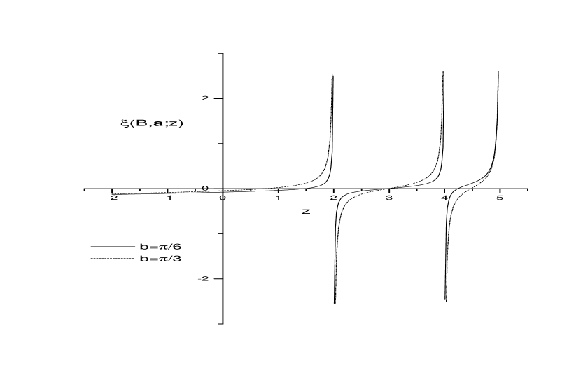
Figure 5: The function $\xi(B,\vec{a};\cdot)$ for $B=1$, $d=\pi$ and $b=\pi/6,\pi/3$.

This is the generical case since the last name property is valid always if the ratio of the coefficients $|B|$ and $(\pi/d)^{2}$ is irrational. If it is rational, then to a given $z_{0}\in\sigma_{ess}(H_{0})$ there may exist different pairs $m_{j},n_{j}$ with the index belonging to a family $J(z_{0})$ such that $|B|(2m_{j}+1)+(\pi n_{j}/d)^{2}=z_{0}$ for all $j\in J(z_{0})$. Taking this degeneracy into account we have

$$\xi(B,\vec{a};z)=-\,{|B|\over\pi d}\>{1\over z-z_{0}}\,\sum_{j\in J(z_{0})}\sin^{2}\left({\pi n_{j}b\over d}\right)\,+\,{\cal O}(1)\,.$$ (4.22)

When $z$ approaches $z_{0}$ from below, $\xi$ diverges to $\infty$, while if it approaches $z_{0}$ from above, $\xi$ goes to $-\infty$. The formula (4.22) also shows that we can disregard those $j$ for which $\sin(\pi n_{j}b/d)=0$: as above the system does not “feel” a point perturbation situated at a transverse eigenfunction node.

To find the behaviour as $z\to-\infty$, recall that the argument leading to the expression (4.16) shows that the latter differs from the non-magnetic formula (2.14) by the replacement $z\to z\!-\!|B|$ together with the addition of terms which remain bounded as $z\to-\infty$. Consequently, the asymptotics is independent of $B$ and given by the formula

$$\xi(B,\vec{a};z)=-\,{\sqrt{-z}\over 4\pi}\,+\,{\cal O}(1)\qquad{\rm as}\qquad z\to-\infty.$$ (4.23)

Having discussed the properties of the function $\xi$, we can apply the conclusions on the equation (4.19). Since $\xi$ is strictly increasing between every pair of neighbouring singularities, there is a unique eigenvalue $\varepsilon_{r}(B,\alpha,\vec{a})$ in each gap for any $\alpha\in\mathbb{R}$ and it satisfies the inequality

$$\varepsilon_{r}(B,\alpha,\vec{a})>\varepsilon_{r}(B,\alpha^{\prime},\vec{a})\qquad{\rm if}\qquad\alpha>\alpha^{\prime},$$

where the index $r$ is labeling the gaps of $H_{0}$. The value $r=0\,$ corresponds to the interval $(-\infty,|B|+(\pi/d)^{2})$, $\,r=1\,$ represents the first finite gap with the left endpoint $|B|+(\pi/d)^{2}$, etc.

Since we know the behaviour of $\xi$ around the singularities, we can write the explicit expression of $\varepsilon_{r}(B,\alpha,\vec{a})$ in the limits of strong and weak coupling. Suppose that the point $|B|(2m_{j}+1)+(\pi n_{j}/d)^{2}=z_{0}\in\sigma_{ess}(H_{0})$ separates the $r$-th and $(r\!+\!1)$-th gap, then using the implicit-function theorem we get

$$\varepsilon_{r}(B,\alpha,\vec{a}) = z_{0}-{1\over\alpha}\,{|B|\over\pi d}\,\sum_{j\in J(z_{0})}\sin^{2}\left({\pi n_{j}b\over d}\right)$$ (4.24)

$$+\,{\cal O}(\alpha^{-2})\qquad{\rm as}\qquad\alpha\to\infty\,,$$

$$\varepsilon_{r+1}(B,\alpha,\vec{a}) = z_{0}-\,{1\over\alpha}\,{|B|\over\pi d}\,\sum_{j\in J(z_{0})}\sin^{2}\left({\pi n_{j}b\over d}\right)$$

$$+\,{\cal O}(\alpha^{-2})\qquad{\rm as}\qquad\alpha\to-\infty\,.$$

We see that the strong and weak limits are similar in the magnetic case. A different behaviour we find only for the lowest eigenvalue for which the asymptotic formula (4.23) gives

$$\varepsilon_{0}(B,\alpha,\vec{a})=-16\pi^{2}\alpha^{2}(1+{\cal O}(\alpha^{-1}))\qquad{\rm as}\qquad\alpha\to-\infty\,.$$ (4.25)

A finer estimate with the error term replaced by ${\cal O}(\alpha^{-2})$ can be obtained when the $\xi$ is expressed in terms of the Hurwitz $\zeta$-function – see, e.g., [17]. As in the non-magnetic case, the residuum of the resolvent pole in the formula (4.12) yields a (non-normalized) eigenfunction

$$\psi(\vec{x};\alpha,\vec{a})=G^{B}_{0}(\vec{x},\vec{a};\varepsilon_{r}(B,\alpha,\vec{a}))$$ (4.26)

corresponding to $\varepsilon_{r}(B,\alpha,\vec{a})$, where $G^{B}_{0}$ is the free resolvent (4.2).

We are naturally interested in the behaviour of the eigenfunction in the limit $|\alpha|\to\infty$ for eigenvalues satisfying the asymptotic relations (4.24). In the both cases, by [20, 1.17.11] the gamma functions in the sum (4.2) corresponding to $n_{j},\;j\in J(z_{0})\,$ diverges as

$$\Gamma(-m_{j}+\epsilon)\,=\,{(-1)^{m_{j}}\over m_{j}!}\>{1\over\epsilon}\,+\,{\cal O}(1)\qquad{\rm as}\qquad\epsilon\to 0\,.$$

This makes it possible to write the leading term of the asymptotics explicitly,

$$\psi(\vec{x};\alpha,\vec{a}) \!=\! {\alpha\over\sum_{j\in J(z_{0})}\sin^{2}\left({\pi n_{j}b\over d}\right)}\>\Phi^{B}(x,x^{\prime})$$

$$\!\!\!\!\!\times\sum_{j\in J(z_{0})}U\left(-m_{j}+{1\over\alpha}\,{1\over 2\pi d}\sum_{j\in J(z_{0})}\sin^{2}\left({\pi n_{j}b\over d}\right),1;{|B|\over 2}\,|x-a|^{2}\right)$$

$$\!\!\!\!\!\times\>{(-1)^{m_{j}}\over m_{j}!}\,\sin\left({\pi n_{j}b\over d}\right)\sin\left({\pi n_{j}y\over d}\right)\,+\,{\cal O}(1)\qquad{\rm as}\quad|\alpha|\to\infty\,.$$

By [9, 13.6.27] the hypergeometric function is reduced to a Laguerre polynomial,

$$U(-n,1,u)=(-1)^{n}n!L_{n}(u)\,,$$

at positive-integer values of the first index, so the wave function can be rewritten as

$$\psi(\vec{x};\alpha,\vec{a}) \approx {\alpha\over\sum_{j\in J(z_{0})}\sin^{2}\left({\pi n_{j}b\over d}\right)}\,\Phi^{B}(x,a)$$

$$\times\sum_{j\in J(z_{0})}L_{m_{j}}\left({|B|\over 2}|x-a|^{2}\right)\sin\left({\pi n_{j}b\over d}\right)\sin\left({\pi n_{j}y\over d}\right).$$

In the last formula we have not specified the error term which has an extra part coming from the variation of the hypergeometric function $U(\cdot,1,u)$ around integer values.

We stated that the eigenvalue $\varepsilon_{0}(B,\alpha,\vec{a})$ in the strong coupling limit case has the same behavior as if there were no magnetic field. The same is true for the corresponding eigenfunction which is strongly localized,

$$\psi(\vec{x};\alpha,\vec{a}) = {1\over d}\,\Phi^{B}(x,a)\sum_{n=1}^{\infty}\left(2\pi\sqrt{|B|+16\pi^{2}\alpha^{2}+\left({\pi n\over d}\right)^{2}}|x-a|\right)^{-1/2}$$

$$\!\!\!\times e^{-\sqrt{|B|+16\pi^{2}\alpha^{2}+\left({\pi n\over d}\right)^{2}}|x-a|}\sin\left({\pi ny\over d}\right)\sin\left({\pi nb\over d}\right)+{\cal O}(\alpha^{-1}).$$

Let us summarize the results obtained for the layer in the magnetic field with one point interaction.

Theorem 4.4

Let $H^{B}(\alpha,\vec{a})$ be defined by (4.2) and (4.2); then
(a) $\sigma_{ess}(H^{B}(\alpha,\vec{a}))=\left\{|B|(2m+1)+(\pi n/d)^{2}\,:\;m,n-1\in\mathbb{N}_{0}\right\}$.
(b) For any $\alpha\in\mathbb{R}$ there exists a single eigenvalue $\varepsilon_{r}(B,\alpha,\vec{a})$ between every two neighbouring values from the essential spectrum, with the exception of the case when the leading term coefficient in (4.22) is zero and the eigenvalue coincides with the Landau in question for a particular value of $\alpha$. Each of these eigenvalues is increasing and infinitely differentiable w.r.t. $\alpha$. The corresponding eigenfunction is given by (4.26).
(c) In the both limits $\alpha\to\pm\infty$ the eigenvalue behaves similarly according to (4.24), except for the strong coupling limit for the lowest eigenvalue, where the formula (4.25) is valid. The eigenfunctions corresponding to the eigenvalues (4.24) and (4.25) are given by (4.3) and (4.3), respectively.

4.4 Finite number of point interactions

Next we consider a finite number $N$ of point interactions supported by points $\vec{a}_{j},\;j=1,\ldots,N$. We define the Hamiltonian in a way similar to that of Sec. 3, i.e. it will be given by (4.2) and (4.2), where $\vec{a}$, $\alpha$ are again shorthands for $\vec{a}=(\vec{a}_{1},\ldots,\vec{a}_{N})$ and $\alpha=(\alpha_{1},\ldots,\alpha_{N})$, and instead of a single boundary condition there is an $N$-tuple of them,

$$L_{1}(\psi,\vec{a}_{j})-4\pi\alpha_{j}L_{0}(\psi,\vec{a}_{j})=0\,,\qquad j=1,\ldots,N\,.$$ (4.30)

Accordingly, the Krein’s formula reads

$$(H^{B}(\alpha,\vec{a})-z)^{-1}(\vec{x},\vec{x}^{\prime})$$ (4.31)

$$=\,G^{B}_{0}(\vec{x},\vec{x}^{\prime};z)\,+\,\sum_{j,k=1}^{N}\lambda_{jk}(B,\alpha,\vec{a};z)\,G^{B}_{0}(\vec{x},\vec{a}_{j};z)\,G^{B}_{0}(\vec{a}_{k},\vec{x}^{\prime};z)\,.\phantom{AAA}$$

Repeating the argument of Sec. 3.2, we find $\lambda(B,\alpha,\vec{a};z)^{-1}=\Lambda(B,\alpha,\vec{a};z)$ with

$$\Lambda_{mj}(B,\alpha,\vec{a};z):=\delta_{jm}(\alpha_{m}-\xi(B,\vec{a}_{m};z))-(1-\delta_{jm})G^{B}_{0}(\vec{a}_{m},\vec{a}_{j};z)\,,$$ (4.32)

or more explicitly by means of (4.16) and (4.2)

$$\Lambda_{jj} = \alpha_{j}-\,{1\over 2\pi d}\,\sum_{n=1}^{\infty}\left[\,\ln\left((\pi n)^{2}\over 2|B|d^{2}\right)-\psi\left({|B|-k^{2}_{n}(z)\over 2|B|}\right)\right]\sin^{2}\left({\pi nb_{j}\over d}\right)$$ (4.33)

$$-\,{1\over 4\pi d}\,\left[\,\gamma+\psi\left({b_{j}\over d}\right)+{\pi\over 2}\cot\left({\pi b_{j}\over d}\right)\right]$$

and

$$\Lambda_{mj} = -\,{1\over 2\pi d}\,\Phi^{B}(a_{m},a_{j})\,\sum_{n=1}^{\infty}\>\Gamma\left({|B|-k^{2}_{n}(z)\over 2|B|}\right)$$

$$\times\>U\left({|B|-k^{2}_{n}(z)\over 2|B|},1;{|B|\over 2}\,|a_{m}-a_{j}|^{2}\right)\sin\left({\pi nb_{j}\over d}\right)\sin\left({\pi nb_{m}\over d}\right)$$

for $j\neq m$. If some perturbations are arranged vertically, $a_{j}=a_{m}$ for $j\neq m$, the last expression can be written as

$$\Lambda_{mj} = \,-\,{1\over 2\pi d}\sum_{n=1}^{\infty}\left[\,\ln\left((\pi n)^{2}\over 2|B|d^{2}\right)-\psi\left({|B|-z+\left({\pi n\over d}\right)^{2}\over 2|B|}\right)\right]$$

$$\times\sin\left({\pi nb_{m}\over d}\right)\sin\left({\pi nb_{j}\over d}\right)$$

$$-\,\xi_{2}\left({b_{j}+b_{m}\over 2}\right)\,+\,\xi_{2}\left({|b_{j}-b_{m}|\over 2}\right)$$

as we find by a direct modification of the argument yielding $\xi(B,\vec{a};z)$.

Consider again a point $z_{0}\in\sigma_{ess}(H_{0})$. If $z$ approaches this value, the appropriate contributions to the sums in (4.16) and (4.2) diverge and the matrix elements of $\Lambda$ behave in the limit $z\to z_{0}$ as

$$\Lambda_{jj} = \alpha_{j}-\,{|B|\over\pi d}\,{1\over z_{0}-z}\,\sum_{i\in J(z_{0})}\,\sin^{2}\left({\pi n_{i}b_{j}\over d}\right)\,+\,{\cal O}(1)\,,$$ (4.36)

$$\Lambda_{mj} = -\,{|B|\over\pi d}\>\Phi^{B}(\vec{a}_{m},\vec{a}_{j})\,{1\over z_{0}-z}$$

$$\times\>\sum_{i\in J(z_{0})}{(-1)^{m_{i}}\over m_{i}!}\>U\left({|B|+\left({\pi n_{i}\over d}\right)^{2}-z\over 2|B|},1;{|B|\over 2}\,|a_{j}-a_{m}|^{2}\right)$$

$$\phantom{AA}\times\>\sin\left({\pi n_{i}b_{j}\over d}\right)\sin\left({\pi n_{i}b_{m}\over d}\right)\,+\,{\cal O}(1)\quad\mathrm{if}\quad j\neq m\,,$$

$$\Lambda_{mj} = -\,{|B|\over\pi d}\,{1\over z_{0}-z}\sum_{i\in J(z_{0})}\,\sin\left({\pi n_{i}b_{j}\over d}\right)\sin\left({\pi n_{i}b_{m}\over d}\right)\,+\,{\cal O}(1)$$

$$\quad\mathrm{if}\quad j\neq m\ ,\;a_{j}=a_{m}\,.$$

Moreover, the hypergeometric functions reduce to the Laguerre polynomials in the limit, so

$$\Lambda_{mj} \approx -{|B|\over\pi d}\Phi^{B}(a_{m},a_{j}){1\over z_{0}-z}$$

$$\times\sum_{i\in J(z_{0})}L_{m_{i}}\left({|B|\over 2}|a_{m}-a_{j}|^{2}\right)\sin\left({\pi n_{i}b_{j}\over d}\right)\sin\left({\pi n_{i}b_{m}\over d}\right).$$

For large negative energies, $z\to-\infty$, we employ the asymptotic behavior of $\xi$ given by (4.23) arriving thus at

$$\Lambda_{jj}=\alpha_{j}\,+\,{\sqrt{-z}\over 4\pi}\,+\,{\cal O}(1)$$ (4.38)

with $B$-dependence being hidden in the error term. The non-diagonal part of the matrix $\Lambda$ vanishes in the limit of large negative energy, because by [9, 13.3.3] one has

$$\Lambda_{mj} \approx -\,{1\over 2\pi d}\>\Phi^{B}(\vec{a}_{m},\vec{a}_{j})\>\sum_{n=1}^{\infty}K_{0}\left(\sqrt{|B|-k^{2}_{n}(z)}|a_{m}-a_{j}|\right)$$

$$\phantom{AAAAAAAAAAAA}\times\sin\left({\pi nb_{j}\over d}\right)\sin\left({\pi nb_{m}\over d}\right)\,,$$

which is exponentially decreasing, $K_{0}(s)\approx\sqrt{{\pi\over 2s}}\>e^{-s}\>$ as $s\to\infty\,$. In the case of a vertical arrangement, $a_{j}=a_{m}$ for $j\neq m$, we can again claim only that the matrix element $\Lambda_{jm}$ is bounded.

Having obtained the coefficient matrix $\Lambda(B,\alpha,\vec{a};z)$ given by (4.33) and (4.4) we proceed with finding the eigenvalues (the essential spectrum is preserved, of course). In the same way as in Sec. 3.3 we check that an eigenvalue $z$ is a solution of the implicit equation

$$\det\Lambda(B,\alpha,\vec{a};z)\,=\,0$$ (4.39)

and the corresponding eigenfunction can be written as

$$\varphi(\vec{x})=\sum_{j=1}^{N}d_{j}G^{B}_{0}(\vec{x},\vec{a}_{j};z)\,,$$ (4.40)

where $d:=(d_{1},\ldots,d_{N})$ is an eigenvector of the matrix $\Lambda(B,\alpha,\vec{a};z)$.

As in the Sec.4.3 we would like to say something about the number of eigenvalues in each gap. We already know that this number is limited from above by $N$. Denoting $\alpha_{j}=\widetilde{\alpha}_{j}+\bar{\alpha}$ we can split the matrix $\Lambda(z,\alpha)$ into two parts

$$\Lambda(z,\alpha)\,=\,\bar{\alpha}I-M(z,\widetilde{\alpha})\,,$$ (4.41)

where $\widetilde{\alpha}:=(\widetilde{\alpha}_{1},\ldots,\widetilde{\alpha}_{N})$. The explicit form of the matrix $M$ can be obtained from the relations (4.33) and (4.4) by changing the signs and substituting $\alpha_{j}$ by $\widetilde{\alpha}_{j}$. The same can be done for the formulae (4.36) which express the behavior around the singularity. In the limit $z\to z_{0}$ one can neglect the parameters $\widetilde{\alpha}_{j}$’s, then it is possible to write

$$M(z,\widetilde{\alpha})={1\over z_{0}-z}\,{|B|\over\pi d}\,\bar{M}(z_{0})\,+\,{\cal O}(1)\,,$$

where

$$\bar{M}_{jj}(z_{0}) = \sum_{i\in J(z_{0})}\,\sin^{2}\left({\pi n_{i}b_{j}\over d}\right)$$

$$\bar{M}_{mj}(z_{0}) = \Phi_{B}(\vec{a}_{m},\vec{a}_{j})\sum_{i\in J(z_{0})}\,L_{m_{i}}\left({|B|\over 2}|a_{m}-a_{j}|^{2}\right)$$

$$\phantom{AAAAAAAAA}\times\sin\left({\pi n_{i}b_{j}\over d}\right)\,\sin\left({\pi n_{i}b_{m}\over d}\right).$$

Following [21] the eigenvalues of $\Lambda(z)$ monotonously increase between two neighbouring singularities. Then all eigenvalues of $\bar{M}$ are non-negative numbers. For $\sum_{j=1}^{N}\sum_{i\in J(z_{0})}\sin^{2}(\pi n_{i}b_{j}/d)\neq 0$ at least one is positive, hence at least one eigenvalue of the matrix $M(z,\widetilde{\alpha})$ diverge to $-\infty$ or to $\infty$ as $z\to z_{0+}$, $z\to z_{0-}$ respectively. Let us summarize the results:

Theorem 4.5

Let the operator $H^{B}(\alpha,\vec{a})$ be defined by (4.2) and (4.2), where $\vec{a}=(\vec{a}_{1},\ldots,\vec{a}_{N})$ and $\alpha=(\alpha_{1},\ldots,\alpha_{N})$ and the boundary condition is replaced by(4.30); then
(a) $\sigma_{ess}(H^{B}(\alpha,\vec{a}))=\left\{|B|(2m+1)+(\pi n/d)^{2}\,:\;m,n-1\in\mathbb{N}_{0}\right\}$.
(b) For any $\alpha\in\mathbb{R}^{N}$ there exists at most $N$ eigenvaluee between every two neighbouring values from the essential spectrum with the multiplicity taken into account. The corresponding eigenfunctions are given by (4.40).
(c) In the limits $\min_{1\leq j\leq N}\alpha_{j}\to\infty$ and $\max_{1\leq j\leq N}\alpha_{j}\to-\infty$ at least one eigenvalue converges to each value $z_{0}$ from the essential spectrum from below and from above, respectively, with the exception of the case when the leading term coefficients in (4.36) are zero. In the strong limit case there are also $N$ eigenvalues given by (4.25) with corresponding eigenfunctions given by (4.3), where $\alpha$ and $\vec{a}$ is replaced by $\alpha_{j}$ and $\vec{a}_{j}$ for $j=1\ldots N$.

Further results on the number of eigenvalues of the Hamiltonian $H_{0}^{B}$ can be obtained in the same way as in [23].

Remark 4.6

If some of the point interactions are vertically arranged, we cannot exclude that eigenvalues are absent in a particular gap for some $\alpha$.

Consider two point interactions placed at $(0,0,1/4d)$ and $(0,0,2/3d)$ with $\widetilde{\alpha}_{1}=\widetilde{\alpha}_{2}=0$. The numerical calculation for $B=1$ and $d=\pi$ shows that the eigenvalues of matrix $M(z,\widetilde{\alpha})$ for $z\in(z_{0}(1,1),z_{0}(0,2))$ cover whole $\mathbb{R}$ except one gap, see Fig.  6. The symbol $z_{0}(m,n)$ represents the Landau level $z_{0}=|B|(2m+1)+(\pi n/d)^{2}$. Hence for $\bar{\alpha}$ from this gap the matrix $\Lambda$ has no eigenvalue in the interval $(z_{0}(1,1),z_{0}(0,2))=(4,5)$.

Figure 6: The behavior of two eigenvalues of the matrix $M(z,\widetilde{\alpha})$ for $z\in(4,5)$.

5 Conclusions

We have analyzed here spectral and scattering properties of a hard-wall layer with a finite number of point interactions. The results offer one more illustration of efficiency of Krein’s formula which allows to reduce the task in fact to an algebraic problem. There are other interesting question related to systems with finitely many perturbations such as relations between the perturbation configurations and the spectra including the nodal structure, etc., positions of resonances including those coming from perturbation of the embedded eigenvalues, and so on. To keep this paper within reasonable limits, however, we postpone these questions to a sequel.

The same applies to systems with an infinite number of point obstacles which offer a wider variety of spectral types. Let us briefly mention several problems which we regard as worth of attention. One of them concerns the number of gaps in periodic systems. A periodic layer of point interactions in $\mathbb{R}^{3}$ has at most one gap [2, Sec. III.1]. On the other hand it is known that the presence of boundaries can enhance the number of gaps in the two-dimensional case [5]; a similar effect is expected in dimension three: for a thin enough layer there will be many open gaps between the first and the second transverse threshold. A more difficult question concerns the validity of the Bohr-Sommerfeld conjecture in such systems.

Even more interesting are spectral properties of periodically perturbed layers in presence of a magnetic field. It is well known that a combination of a square lattice of point interactions and a homogeneous magnetic field leads to a very rich spectrum whose properties depend substantially on the number-theoretical properties of the ratio between the lattice spacing and the field intensity (which determines the cyclotronic radius) – see [2, Sec. III.2.5] or [24]. Putting such a system into a layer brings a third parameter (the layer width $d$) which will determine how “thickly” the transverse-mode component are overlayed in the spectrum.

The same applies to edge-type states. It was shown recently that an equidistant array of point interaction in combination with a homogeneous magnetic field can produce bands of absolutely continuous spectrum away of the Landau levels [25]. One is naturally interested how the spectrum will change if the array is confined between a pair of hard walls. Other problems concern aperiodic perturbations, external electric field, spin effects, etc.

Acknowledgments

Useful remarks of V. Geyler and P. Šeba are gratefully acknowledged. The research was partially supported by the GAAS grant # 1048801.

References

- [1] E.N. Bulgakov, K.N. Pichugin, A.F. Sadreev, P. Středa, P. Šeba: “Hall-like effect induced by spin-orbit interaction”, Phys. Rev. Lett. 83, 376-379 (1999).
- [2] S. Albeverio, F. Gesztesy, R. Høegh-Krohn, H. Holden: Solvable Models in Quantum Mechanics, Springer, Heidelberg 1988.
- [3] J.T. Londergan, J.P. Carini, D.P. Murdock: Binding and Scattering in Two-Dimensional Systems. Application to Quantum Wires, Waveguides and Photonic Crystals, Springer, Berlin 1999.
- [4] P. Šeba: “Wave chaos in singular quantum billiard”, Phys. Rev. Lett. 64, 1855-1858 (1990).
- [5] P. Exner, R. Gawlista, P. Šeba, M. Tater: “Point interactions in a strip”, Ann. Phys. 252, 133-179 (1996).
- [6] P. Exner: “Point interactions in a tube”, in Proceedings of the Conference “Infinite-dimensional Stochastic Analysis” (Leipzig 1999); Canadian Mathematical Society, to appear
- [7] M. Reed and B. Simon: Methods of Modern Mathematical Physics, II. Fourier Analysis. Self-Adjointness, III. Scattering Theory, IV. Analysis of Operators, Academic Press, New York 1975–1979.
- [8] E.C. Titchmarch: Eigenfunction Expansions Associated with Second-Order Differential Equations, vol.II, Clarendon Press, Oxford 1958.
- [9] M.S. Abramowitz, I.A. Stegun, eds.: Handbook of Mathematical Functions, Dover, New York 1965.
- [10] A.P. Prudnikov, Yu.O. Brychkov, O.I. Marichev: Integraly i rady, I. Elementarnye funkcii, II. Specialnye funkcii, Nauka, Moskva 1981–1983.
- [11] J. Weidman: Linear Operators in Hilbert Spaces, Springer, New York 1980.
- [12] V. Jarník: Differential Calculus I (in Czech), Academia, Prague 1984.
- [13] J. Blank, P. Exner, M. Havlíček: Hilbert Space Operators in Quantum Physics, American Institute of Physics, New York 1994.
- [14] V.V. Dodonov, I.A. Malkin, V.I. Man’ko: “The Green function of the stationary Schrödinger equation for a particle in a uniform magnetic field”, Phys. Lett. A51, 133-134 (1975).
- [15] Yu.M. Berezanskii: Eigenfunction Expansions for Self-Adjoint Operators (in Russian), Naukova Dumka, Kiev 1965.
- [16] V.A. Geyler, V.V. Demidov: “On the Green function of the Landau operator and its properties related to point interactions”, J. Anal. Appl. 15, 851-863 (1996).
- [17] S. Albeverio, V.A. Geyler, O.G. Kostrov: “Quasi–one–dimensional nanosystems in a uniform magnetic field: explicitly solvable model”, Rep. Math. Phys. 44, 13-20 (1999).
- [18] Y.N. Demkov, V.N. Ostrovsky: The Use of Zero-Range Potentials in Atomic Physics (in Russian), Nauka, Moscow 1975.
- [19] C. Miranda: Partial Differential Equations of Elliptic Type, Springer, New York 1970
- [20] H. Bateman, A. Erdelyi: Higher Transcendental Functions, I. Hypergeometric Function, Legendre Functions, McGraw-Hill, New York 1953.
- [21] M.G. Krein, G.K. Langer: “O defektnych podprostranstvach ermitova operatora”, Funct.Anal.Appl. 5, 59-71 (1971)
- [22] F. Gesztesy, H. Holden, P. Šeba: “On point interactions in magnetic field system”, in Schrödinger Operators, Standard and Non-standard (P. Exner, P. Šeba, eds.), World Scientific, Singapore 1989; pp. 147-164
- [23] S. Albeverio, V.A. Geyler: “The Band Structure of the General Periodic Schrödinger Operator with Point Interactions”, Commun. Math. Phys. 210, 29-48 (2000)
- [24] M.A. Shubin: “Discrete magnetic Laplacian”, Commun. Math. Phys. 164, 259-275 (1994).
- [25] P. Exner, A. Joye, H. Kovařík: “Edge currents in the absence of edges”, Phys. Lett. A264, 124-130 (1999).