Abstract

This paper is a direct illustration of a construction of coherent states which has been recently proposed by two of us (JPG and JK). We have chosen the example of a particle trapped in an infinite square-well and also in Pöschl-Teller potentials of the trigonometric type. In the construction of the corresponding coherent states, we take advantage of the simplicity of the solutions, which ultimately stems from the fact they share a common $SU(1,1)$ symmetry à la Barut–Girardello. Many properties of these states are then studied, both from mathematical and from physical points of view.

PACS: 02.30.Tb, 02.90.+p, 03.65.-w, 31.15.-p

I INTRODUCTION

Despite its relevance for the understanding of the most elementary parts of quantum mechanics, the problem of a particle trapped in an infinite square-well (Figure 1) usually deserves no more than a few pages in most physics textbooks [2, 3, 4]. Solutions are straightforward to derive, energy is nicely quantized and trigonometric wave functions afford an immediate intuition of quantum behavior. The model is widely used to give a fair idea of many body systems in atomic or molecular physics. However, very soon one may become puzzled by less trivial problems pertaining to the mathematics of quantum mechanics: domain of self-adjointness for the operators involved, possible nonuniqueness of self-adjoint extensions (see in particular the very instructive examples in Chapters VIII.I, VIII.2, and X.1 of [5]), explicit kernel of the evolution operator, crucial role played by the boundary conditions, semi-classical behavior and the classical limit, and other limiting situations such as a very large or a vanishingly small width of the well.

Actually all these questions can be considered through a nice analytic regularization of the infinite well potential. Indeed, consider the continuously indexed family of potentials

$$V(x)\equiv V_{\lambda,\kappa}(x)=\frac{1}{2}V_{o}\left(\frac{\lambda(\lambda-1)}{\cos^{2}\frac{x}{2a}}+\displaystyle\frac{\kappa(\kappa-1)}{\sin^{2}\frac{x}{2a}}\right),\quad 0\leqslant x\leqslant\pi a,$$ (1.1)

for $\lambda,\kappa>1$ ($V_{o}>0$ is a coupling constant). Clearly this is a smooth approximation, for $\lambda,\kappa\to 1^{+}$, of the infinite square-well over the interval $[0,\pi a]$. These potentials, called the Pöschl–Teller (PT) potentials [4, 6], are shown in Figure 2 for the values $(\lambda,\kappa)=(4,4),(4,8),(4,16)$, respectively. In order to make contact with standard quantum mechanics on the whole line, there are two possibilities. Either one requires that $V(x)=\infty$ outside the interval $[0,\pi a]$, or one periodizes the potential, with period $\pi a$, and one imposes periodic boundary conditions at the points $\{n\pi a,\,n\in{\mathbb{Z}}\}$. But, since the walls separating the successive cells are impenetrable, one may also simply ignore these extensions and consider only the interval $[0,\pi a]$, which we shall do in the present paper.

The Pöschl–Teller potentials share with their infinite well limit the nice property of being analytically integrable. The reason behind this can be understood within a group-theoretical context: The family of potentials (1.1) possesses an underlying dynamical algebra, namely $\mathfrak{su}(1,1)$ and the discrete series representations of the latter. We recall that the discrete series UIR’s of $\mathfrak{su}(1,1)$ are labelled by a parameter $\eta$, which takes its values in $\{\frac{1}{2},1,\frac{3}{2},2,\ldots\}$ for the discrete series stricto sensu, and in $[\frac{1}{2},+\infty)$ for the extension to the universal covering of the group $SU(1,1)$. The relation between the Pöschl–Teller parameters and $\eta$ is given by

$$2\eta-1=\lambda+\kappa,$$

and the limit case $\lambda,\kappa\rightarrow 1^{+}$ corresponds to $\eta=\frac{3}{2}$.

Other approaches in the past led to the group $SU(2)$ as the dynamical group for the Pöschl–Teller potentials, when $\lambda+\kappa$ is an integer [7]. We emphasize here the fact that the $SU(1,1)$ approach seems more natural, for it extends easily and naturally to noninteger values of $\lambda+\kappa$.

Figure 1: The infinite square-well potential.

Figure 2: The Pöschl–Teller potential $V(x)=\frac{1}{2}V_{o}\left[{\lambda(\lambda-1)}{\cos^{-2}\frac{x}{2a}}+{\kappa(\kappa-1)}{\sin^{-2}\frac{x}{2a}}\right],$ with $a=\pi^{-1}$ and for $(\lambda,\kappa)=(4,4),(4,8),(4,16)$ (from bottom to top).

In fact, the Pöschl–Teller potential (1.1), sometimes called PT of the first type, is closely related to several other potentials, widely used in molecular and solid state physics.

• The symmetric Pöschl–Teller potential well, given by $\lambda=\kappa\geqslant 1$,

  $$V_{\lambda}(x)=2V_{o}\displaystyle\frac{\lambda(\lambda-1)}{\sin^{2}\frac{x}{a}}\ .$$ (1.2)

  This potential may be periodized with period $\pi a/2$, instead of $\pi a$.

• The same potential, for $\frac{1}{2}\leqslant\lambda<1$, is known as the Scarf potential [8]. This is no longer a well, but an inverted well, that is, a peak between two infinite negative wells. When periodized over the whole line, this a good model for a 1-D crystal (as a smooth substitute to the well-known Kronig-Penney model), since the spectrum of the corresponding Hamiltonian has a band structure. The nonsymmetric extension of the Scarf potential has similar properties [9]. Interestingly, both cases admit $SU(1,1)$ as dynamical group, although the representations underlying the band part are those of the complementary series.

• There exists also the so-called scattering (or modified) Pöschl–Teller potentials, obtained by replacing the trigonometric functions in (1.1) by their hyperbolic counterparts [6]. A special case is the Rosen–Morse potential [10], which is simply the symmetric version of the previous one. These potentials are widely used in molecular physics, and they have the same dynamical group $SU(1,1)$ (but again other representations are involved). For a review of this case and its applications, we refer to [11, 12, 13].

In this paper we present and study families of coherent states (CS) adapted to the infinite well and to the Pöschl–Teller potentials. We call these states adapted and coherent because they are a direct generalization of the standard ones corresponding to the harmonic oscillator [14] (for an extensive and up-to-date bibliography see, for instance, [15]). We recall that the Schrödinger–Klauder–Glauber CS read

$$|z\rangle=e^{-\frac{|z|^{2}}{2}}\sum_{n\geqslant 0}\frac{z^{n}}{\sqrt{n!}}\;|n\rangle.$$ (1.3)

We extend them in a sense already explained in [16, 17, 18] and briefly sketched in the following. We first consider in (1.3) the kets $|n\rangle$ as the eigenstates of the infinite well (resp. Pöschl–Teller) Hamiltonian $H$ corresponding to the eigenvalue $\hbar\omega e_{n}$, $n\geq 0,e_{0}=0$. Next, analogous to the pioneering work of Jackson [19], we replace in the square root the factorial $n!$ by the generalized factorial $[e_{n}]!=e_{1}\cdots e_{n}$, to get the so-called action identity [17]

$$\langle z|H|z\rangle=\hbar\omega|z|^{2}.$$ (1.4)

Note that similar factorial “deformations” in the construction of coherent states already appear in [20, 21]. We finally require (temporal) stability for our new family of coherent states under the action of the evolution operator $e^{-iHt/\hbar}$ (see [17] and Section VII below for details). Our interest for these infinite well and Pöschl–Teller coherent states lies mostly in the simplicity of the formulas involved. We have here at our disposal a nice tool for examining many quantum features, such as probability densities, autocorrelation, mean values of observables, Heisenberg inequalites, semi-classical limits, and others.

The paper is organized as follows. In Section II, we describe the classical motion in an infinite square-well potential and in a Pöschl–Teller potential. In our opinion, it is essential to recall this elementary (and pedagogical!) material for the subsequent discussions on a quantum level. Sections III and IV are devoted to the quantum infinite well and Pöschl–Teller potentials, respectively. In particular, we give here an up-to-date survey of the nontrivial questions of self-adjointness for some of the most familiar physical observables. We examine in Section V the questions related to various limits: semiclassical $\hbar\,\rightarrow\,0,\ n\hbar=\mbox{const}$, infinite narrowness $a\,\rightarrow\,0$, infinite width $a\,\rightarrow\,\infty$, Pöschl–Teller $\rightarrow$ infinite well, and others. We describe in Section VI the dynamical symmetry algebra ${\mathfrak{su}}(1,1)$ common to both models and underlying their integrability. In Section VII we first review the general construction of “action–angle” or rather “energy–time” coherent states before giving their explicit form and their most immediate mathematical properties in the infinite well case, and in the Pöschl–Teller case (Section VIII). Section IX is devoted to the most interesting physical properties of our states, and in particular to the revival features they present, which are well illustrated by the large number of figures shown there. Finally, Section X summarizes the discussion about the role of coherent states when expressed in terms of action–angle variables.

A final lesson of the paper is that a comprehensive study of quantum mechanics requires not only algebra, or numerical simulations, but also a precise use of functional analysis. The fine points of the latter are not mathematical pedantry, they express deep physical properties.

II THE CLASSICAL PROBLEM

A. Classical infinite well

It is worthwhile to start out this paper by a short pedagogical review of the classical behavior of a particle of mass $m$ trapped in an infinite well of width $\pi a$.

For a nonzero energy

$$E=\frac{1}{2}mv^{2},$$ (2.1)

there corresponds a speed

$$v=\sqrt{\frac{2E}{m}}$$ (2.2)

for a position $0<x<\pi a$. There are perfect reflections at the boundaries of the well. So the motion is periodic with period (the “round trip time”) $T$ equal to

$$T=\frac{2\pi a}{v}=2\pi a\sqrt{\frac{m}{2E}}.$$ (2.3)

With the initial condition $x(0)=0$, the time behavior of the position is then given by (see Figure 3)

$$0\leqslant t\leqslant\frac{1}{2}T :\quad x=vt,$$

$$\frac{1}{2}T\leqslant t\leqslant T :\quad x=2\pi a-vt,$$ (2.4)

and of course

$$x(t+nT)=x(t).$$ (2.5)

Consequently the velocity is a periodized Haar function (Figure 4):

$$\mbox{\boldmath$v$}=v\sum_{n=0}^{+\infty}\left[{1\raisebox{1.90633pt}{$\scriptstyle|$}}_{[nT,(n+\frac{1}{2})T]}-{{1\raisebox{1.90633pt}{$\scriptstyle|$}}}_{[(n+\frac{1}{2})T,(n+1)T]}\right]$$ (2.6)

(here ${1\raisebox{1.90633pt}{$\scriptstyle|$}}_{B}$ denotes the characteristic function of a set $B\in{\mathbb{R}}$), whereas the acceleration is the superposition of two Dirac combs on the half-line (Figure 5):

$$\mbox{\boldmath$\gamma$}=\sum_{n=0}^{+\infty}\left[\delta_{nT}-\delta_{(n+\frac{1}{2})T}\right].$$ (2.7)

Figure 3: The position $x(t)$ of the particle trapped in the infinite square-well of width $\pi a$, as a function of time.

Figure 4: The velocity $\mbox{\boldmath$v$}(t)$ of the particle in the infinite square-well: periodized Haar function.

Figure 5: The acceleration $\gamma$(t) of the particle of the particle in the infinite square-well.

Figure 6: Phase trajectory of the particle in the infinite square-well.

The average position and average velocity of the particule are then

$$\overline{x}=\frac{1}{T}\int_{0}^{T}x(t)\,dt=\frac{\pi a}{2},\qquad\overline{v}=0,$$ (2.8)

whereas the mean square dispersions are

$$\sqrt{\overline{x^{2}}-\overline{x}^{2}}=\frac{\pi a}{2\sqrt{3}},\qquad\sqrt{\overline{v^{2}}-\overline{v}^{2}}=\sqrt{\frac{2E}{m}}.$$ (2.9)

Note the standard Fourier expansion for the position and the velocity, respectively,

$$x(t) = \frac{\pi a}{2}-\frac{4a}{\pi}\sum_{n=0}^{\infty}\frac{1}{(2n+1)^{2}}\cos\frac{2\pi}{T}(2n+1)t,$$ (2.10)

$$\mbox{\boldmath$v$}(t) = 4\frac{v}{\pi}\sum_{n=0}^{\infty}\frac{1}{2n+1}\sin\frac{2\pi}{T}(2n+1)t.$$ (2.11)

Figure 6 shows the phase trajectory of the system. This trajectory encircles a surface of area equal to the action variable

$$A=\frac{1}{2\pi}\oint pdq=mva,$$ (2.12)

where $q=x$ and $p=mv$ are canonically conjugate. Note the other expressions for $A$:

$$A=\frac{2\pi a^{2}m}{T}=\frac{mv^{2}T}{2\pi}=a\sqrt{2mE}.$$ (2.13)

The action-angle variables $(A,\varphi)$ are obtained through the canonical transformation ($\vartheta$ denotes the step function)

$$\varphi = {\rm sgn}(p)\frac{q}{a}+\vartheta(-p)2\pi\quad({\rm mod}\,2\pi),$$ (2.14)

$$A = |p|a,$$ (2.15)

with generating function equal to the Maupertuis action, as should be expected:

$$S_{o} = 2\pi nA+S_{o}^{princ}$$

$$S_{o}^{princ} = A\varphi,\quad\varphi\in(0,2\pi)$$ (2.16)

$$= pq+|p|\vartheta(-p)a.$$

Finally, note the time evolution of the angle variable:

$$\varphi=\frac{\mbox{\boldmath$v$}}{a}t+\varphi_{o}\equiv\alpha t+\varphi_{o}.$$ (2.17)

B. Pöschl–Teller potentials

The solution to the equations of motion with the potentials (1.1) is straightforward, in spite of the rather heavy expression of the latter. The turning points $x_{\pm}$ of the periodic motion at a given energy $E$ are given by

$$x_{\pm}=a\;\arccos\left[\frac{\alpha-\beta}{2}\pm\sqrt{\Delta}\right]$$ (2.18)

where $\Delta=(1-\frac{1}{2}(\sqrt{\alpha}+\sqrt{\beta})^{2})(1-\frac{1}{2}(\sqrt{\alpha}-\sqrt{\beta})^{2})$, $\alpha=\displaystyle\frac{V_{0}}{E}\lambda(\lambda-1)$, $\beta=\displaystyle\frac{V_{0}}{E}\kappa(\kappa-1)$.

So the motion is possible only if

$$E>\frac{V_{0}}{2}(\sqrt{\lambda(\lambda-1)}+\sqrt{\kappa(\kappa-1)})^{2}.$$ (2.19)

The time evolution of the position is given by

$$x(t) = a\;\arccos\left[\frac{\alpha-\beta}{2}+\sqrt{\Delta}\cos(\sqrt{\frac{2E}{m}}\,\frac{t}{a})\right]\ ,$$ (2.20)

$$x(0) = x_{-}\ .$$

Hence the period is

$$T=2\pi a\,\sqrt{\frac{m}{2E}}\ .$$ (2.21)

It is remarkable that the period $T$ does not depend on the strength $V_{o}$, nor on $\lambda$ and $\kappa$.

The action variable $A$ satisfies the relation $\displaystyle\frac{dA}{dE}=\displaystyle\frac{T}{2\pi}$, and thus

$$A=a\sqrt{2mE}+\mbox{ const }.$$ (2.22)

The constant is determined by the condition that $A=0$ for $E=V_{min}$, that is, const = $-a\sqrt{2mV_{min}}$. The Pöschl–Teller potential $V(x)$ reaches its minimum at the location $x_{o}$ defined by

$$\tan^{2}\frac{x_{o}}{2a}=\sqrt{\frac{\kappa(\kappa-1)}{\lambda(\lambda-1)}}.$$ (2.23)

So we have, in agreement with (2.19),

$$V_{min}=V(x_{o})=\frac{V_{o}}{2}\left[\sqrt{\lambda(\lambda-1)}+\sqrt{\kappa(\kappa-1)}\right]^{2},$$ (2.24)

and consequently,

$$A=a\sqrt{2mE}-a\sqrt{mV_{o}}[\sqrt{\lambda(\lambda-1)}+\sqrt{\kappa(\kappa-1)}].$$ (2.25)

It is worthwhile to compare (2.21) and (2.25) with their respective infinite well counterparts (2.3) and (2.13). We should also check that the time behavior (2.20) of $x(t)$ goes into (2.4) at the limits $\alpha,\beta\to 0$. We give in Figures 7, 8, and 9 the curves for $x(t)$, $\mbox{\boldmath$v$}(t)$ and $\mbox{\boldmath$\gamma$}(t)$, respectively, in the particular symmetric case $\lambda=\kappa=2$, for two different values of the energy, namely, $E=8V_{o}$ and $E=16V_{o}$. Figure 10 shows the corresponding phase trajectory in the plane $(q=x,p=mv)$. Note that, in the general case, the equation for the latter reads (at energy $E$):

$$p=\pm\frac{\sqrt{2mE}}{\sin\frac{q}{a}}\left[1-(\alpha+\beta)+(\alpha-\beta)\cos\frac{q}{a}-\cos^{2}\frac{q}{a}\right]^{1/2}.$$ (2.26)

Finally, let us give the canonical transformation leading to the action-angle variables

$$\varphi = \arccos\frac{1}{\sqrt{\Delta}}\left[\cos\frac{q}{a}-\frac{\alpha-\beta}{2}\right]$$ (2.27)

$$A = a\,[p^{2}+2mV(q)]^{1/2}.$$ (2.28)

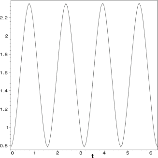
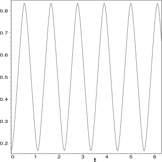
Figure 7: The position $x(t)$ of the particle in the symmetric Pöschl–Teller potential $\lambda=\kappa=2$: (a) $E=8V_{o},\,T=\frac{\pi}{2}$; and (b) $E=16V_{o},\,T=\frac{\pi}{2\sqrt{2}}$ (compare Figure 3).

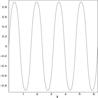
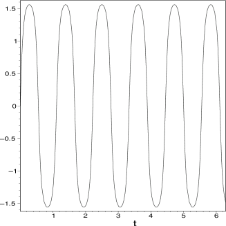
Figure 8: The velocity $\mbox{\boldmath$v$}(t)$ of the particle in the symmetric (2,2) Pöschl–Teller potential, for the same values of $E$ and $T$ as in Figure 7 (compare Figure 4).

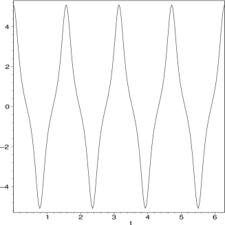
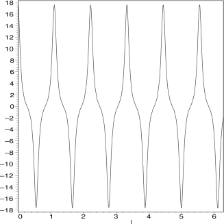
Figure 9: The acceleration $\gamma$$(t)$ of the particle in the symmetric (2,2) Pöschl–Teller potential, for the same values of $E$ and $T$ as in Figure 7 (compare Figure 5).

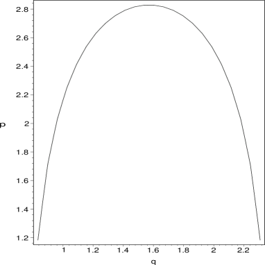
Figure 10: Upper part of the phase trajectory of the particle the symmetric (2,2) Pöschl–Teller system, for the same values of $E$ and $T$ as in Figure 7 (compare Figure 6).

The Maupertuis action generating (2.25) is given by

$$S_{o}(u) = 2\pi nA+S_{o}^{princ}(u),$$

$$S_{o}^{princ}(u) = -a\sqrt{2mE}\int_{u_{-}}^{u}[1-(\alpha+\beta)+(\alpha-\beta)s-s^{2}]^{1/2}\frac{ds}{1-s^{2}}\;$$

with $u=\cos\displaystyle\frac{x}{a}$. The last integral may be calculated explicitly, but the result is not illuminating.

III THE QUANTUM PROBLEM FOR THE INFINITE WELL

Any quantum system trapped inside the infinite well $0\leqslant x\leqslant\pi a$ must have its wave function equal to zero outside the well. It is thus natural to impose on the wave functions the boundary conditions

$$\psi(x)=0,\quad x\geqslant\pi a\quad\mbox{and}\quad x\leqslant 0.$$ (3.1)

Since the movement takes place only inside the interval $[0,\pi a]$, we may as well ignore the rest of the line and replace the conditions (3.1) by the following ones:

$$\psi\in L^{2}([0,\pi a],dx),\quad\psi(0)=\psi(\pi a)=0.$$ (3.2)

Alternatively, one may consider the periodized well and impose the same periodic boundary conditions, namely, $\psi(n\pi a)=0,\,\forall n\in{\mathbb{Z}}$.

In either case, stationary states of the trapped particle of mass $m$ are easily found from the eigenvalue problem for the Schrödinger operator. For reasons to be justified in the sequel, we choose the shifted Hamiltonian:

$$H\equiv H_{\rm w}=-\frac{\hbar^{2}}{2m}\frac{d^{2}}{dx^{2}}-\frac{\hbar^{2}}{2ma^{2}}\ .$$ (3.3)

Then

$$\Psi(x,t)=e^{-\frac{i}{\hbar}Ht}\Psi(x,0),$$ (3.4)

where $\Psi(x,0)\equiv\psi(x)$ obeys the eigenvalue equation

$$H\psi(x)=E\psi(x),$$ (3.5)

together with the boundary conditions (3.1). Normalized eigenstates and corresponding eigenvalues are then given by

$$\psi_{n}(x) = \sqrt{\frac{2}{\pi a}}\sin(n+1)\frac{x}{a}\;\equiv\;\langle x|n\rangle,\quad 0\leqslant x\leqslant\pi a,$$ (3.6)

$$H|n\rangle = E_{n}|n\rangle,\quad n=0,1,\ldots,$$ (3.7)

$$E_{n} = \frac{\hbar^{2}}{2ma^{2}}n(n+2)\;\equiv\;\hbar\omega e_{n},$$ (3.8)

with

$$\omega=\frac{\hbar}{2ma^{2}}\equiv\frac{2\pi}{T_{r}}\quad\mbox{and }\;e_{n}=n(n+2),\quad n=0,1,\ldots,$$

where $T_{r}$ is the “revival” time to be compared with the purely classical round trip time given in (2.3). Now the Bohr-Sommerfeld quantization rule applied to the classical action gives

$$a\sqrt{2mE}=A=(n+1)\hbar,$$ (3.9)

so

$$E={(n+1)^{2}}\frac{\hbar^{2}}{2ma^{2}}=E_{n}+\frac{\hbar^{2}}{2ma^{2}},\;n=0,1,\ldots$$ (3.10)

Thus here the Bohr-Sommerfeld quantization is exact [3], despite the presence of the extra term ${\hbar^{2}}/{2ma^{2}}$ which follows from our particular choice of zero in the energy scale (see (3.3)).

After these elementary considerations, let us have a closer look at the functional analysis of our problem, following mostly [5, 22]. We shall denote by ${\cal H}$ the state space of the infinite well, that is, the closure of the linear span of the orthonormal set $\{|n\rangle,\;n\in{\mathbb{N}}\}$. In the $x$-representation, of course, ${\cal H}=L^{2}([0,\pi a],dx)$. We also denote by $AC(0,\pi a)$ the set of absolutely continuous functions on $[0,\pi a]$ whose derivatives belong to $L^{2}([0,\pi a],dx)$ and by $AC^{2}(0,\pi a)$ the set of functions in $L^{2}([0,\pi a],dx)$ whose weak derivatives are in $AC(0,\pi a)$ (we recall that, roughly speaking, a function is absolutely continuous iff it is the indefinite (Lebesgue) integral of an integrable function).

We begin with the Hamiltonian (3.3). More precisely, we define the infinite well Hamiltonian as the unbounded operator $H\equiv{H}_{\rm w}$ in $L^{2}([0,\pi a],dx)$, acting as (3.3), on the dense domain

$${\cal D}({H}_{\rm w})=\{\psi\in AC^{2}(0,\pi a)\mid\psi(0)=\psi(\pi a)=0\}.$$ (3.11)

On this domain, ${H}_{\rm w}$ is self-adjoint, with purely discrete, nondegenerate spectrum $\{E_{n}=\hbar\omega e_{n},\,n=0,1,\ldots\}$, and the corresponding eigenfunctions $\{\psi_{n},\,n=0,1,\ldots\}$ form an orthonormal basis. Furthermore, the resolvent

$$R_{\rm w}(-\hbar\omega)\equiv({H}_{\rm w}+\hbar\omega)^{-1}=\frac{1}{\hbar\omega}\sum_{n=0}^{\infty}\frac{1}{(n+1)^{2}}|n\rangle\langle n|$$

is a trace-class operator, with trace norm and Hilbert-Schmidt norm, respectively:

$$\|R_{\rm w}(-\hbar\omega)\|_{1} = \frac{1}{\hbar\omega}\sum_{n=0}^{\infty}\frac{1}{(n+1)^{2}}=\frac{\pi^{2}}{6}\,\frac{1}{\hbar\omega},$$

$$\|R_{\rm w}(-\hbar\omega)\|_{2} = \frac{1}{\hbar\omega}\left[\sum_{n=0}^{\infty}\frac{1}{(n+1)^{4}}\right]^{1/2}=\frac{\pi^{2}}{\sqrt{90}}\,\frac{1}{\hbar\omega}.$$

At this stage, it is instructive to compare the Hamiltonian of the infinite well with that of a free particle constrained on a circle of radius $a/2$. Here also, the Hilbert space is $L^{2}([0,\pi a],dx)$. The Hamiltonian ${H}_{\rm c}$ has the same expression as ${H}_{\rm w}\equiv H$, but on the domain

$${\cal D}(H_{\rm c})=\{\psi\in AC^{2}(0,\pi a)\mid\psi(0)=\psi(\pi a),\psi^{\prime}(0)=\psi^{\prime}(\pi a)\},$$ (3.12)

and it is also self-adjoint on its domain. The spectrum is again purely discrete, the eigenvalues coincide with half of those of ${H}_{\rm w}$, namely, $E_{2n-1}=\hbar\omega e_{2n-1},\,n=1,2,\ldots$, but each of them is doubly degenerate, and there is the additional, simple eigenvalue corresponding to $n=0$, namely, $e_{-1}=-1$. The eigenfunctions are

$$\left\{\sqrt{\frac{2}{\pi a}}\sin 2n\frac{x}{a},\;n=1,2,\ldots;\sqrt{\frac{2}{\pi a}}\cos 2n\frac{x}{a},\;n=0,1,2,\ldots\right\},$$ (3.13)

and they constitute another orthonormal basis of $L^{2}([0,\pi a],dx)$. Thus, there exists a unitary correspondence between the two bases (3.6) and (3.13). However, the explicit form of this map rests on the full Hilbert space structure and not only on simple trigonometric identities (see also below).

This is another instance of the well-known fact that the physics is determined by the boundary conditions, not only by the differential expression of the operator.

Now we turn to the canonical position and momentum operators. The position operator is $Q=x$, acting on $L^{2}([0,\pi a],dx)$. It is bounded and self-adjoint. As for the momentum, the natural choice is the operator $P_{o}=-id/dx$, acting on the dense domain

$${\cal D}(P_{o})=\{\psi\in AC(0,\pi a)\mid\psi(0)=\psi(\pi a)=0\}.$$ (3.14)

This operator is closed and symmetric, but not self-adjoint. Since its defect indices are (1,1), $P_{o}$ has self-adjoint extensions, in fact an infinite number of them, indexed by the points of a unit circle, namely $P_{\alpha}=-i\hbar\,d/dx$, acting on the dense domain

$${\cal D}(P_{\alpha})=\{\psi\in AC(0,\pi a)\mid\psi(\pi a)=\alpha\,\psi(0),\;|\alpha|=1\}.$$ (3.15)

For simplicity, we choose $\alpha=1$, that is, periodic boundary conditions. Any other choice $P_{\alpha},\,\alpha\neq 1$, is physically acceptable, and yields similar results.

The operator $P\equiv P_{1}$ is a valid candidate for the momentum observable. Its spectrum is purely discrete and nondegenerate, $\sigma(P)=\{2n\hbar/a,\,n=0,\pm 1,\pm 2,\ldots\}$, with corresponding eigenfunctions $\chi_{n}(x)=1/\sqrt{\pi a}\,\exp(i2nx/a)$. The trouble is that none of these belongs to the domain of the Hamiltonian ${H}_{\rm w}$! And indeed, one has

$$\frac{P^{2}}{2m}\neq{H}_{\rm w}+\frac{\hbar^{2}}{2ma^{2}}\ ,$$ (3.16)

since

$${\cal D}(P^{2})=\{\psi\in AC^{2}(0,\pi a)\mid\psi(0)=\psi(\pi a),\psi^{\prime}(0)=\psi^{\prime}(\pi a)\},$$

so that, up to the constant ${\hbar^{2}}/{2ma^{2}}$, ${P^{2}}/{2m}$ coincides with the Hamiltonian ${H}_{\rm c}$ of a particle on a circle, not ${H}_{\rm w}$!

To conclude, we evaluate the canonical commutation relations (CCR), which take the standard form

$$[Q,P]=i\hbar I,$$ (3.17)

on the domain ${\cal D}(QP)\cap{\cal D}(PQ)={\cal D}(P_{o})$, as given in (3.14). Correspondingly, we obtain the uncertainty relations in the eigenstates $\psi_{n}$ of the Hamiltonian ${H}_{\rm w}$ [compare with the classical case, (2.8) and (2.9)]:

$$\langle Q\rangle_{n} = \frac{\pi a}{2}\ ,$$

$$\langle Q^{2}\rangle_{n} = a^{2}\left(\frac{\pi^{2}}{3}-\frac{1}{2(n+1)^{2}}\right),$$

$$\langle P\rangle_{n} = 0\ ,$$ (3.18)

$$\langle P^{2}\rangle_{n} = \frac{1}{a^{2}}\,\hbar^{2}\,(n+1)^{2}\ ,$$

where $\langle\cdot\rangle_{n}\equiv\langle\psi_{n}\mid\cdot\mid\psi_{n}\rangle$. Note that, in the last relation, $\psi_{n}\in{\cal D}(P)$, but $\psi_{n}\not\in{\cal D}(P^{2})$, so that we really mean $\langle P^{2}\rangle_{n}\equiv\|P\psi_{n}\|^{2}$. Also, according to [4], the relation $\langle P\rangle_{n}=0$ expresses the fact that the current associated to the particle vanishes identically.

Taking all these relations together, we obtain the uncertainties

$$\langle\Delta Q\rangle_{n}^{2} = \langle Q^{2}\rangle_{n}-\langle Q\rangle_{n}^{2}\;=\;a^{2}\left(\frac{\pi^{2}}{12}-\frac{1}{2(n+1)^{2}}\right)\;\geqslant\;a^{2}\left(\frac{\pi^{2}}{12}-\frac{1}{2}\right),$$

$$\langle\Delta P\rangle_{n}^{2} = \langle P^{2}\rangle_{n}-\langle P\rangle_{n}^{2}\;=\;\frac{1}{a^{2}}\,\hbar^{2}\,(n+1)^{2}\;\geqslant\;\frac{\hbar^{2}}{a^{2}}\ ,$$

and the uncertainty relations

$$\langle\Delta Q\rangle_{n}\,\langle\Delta P\rangle_{n}=\hbar\left(\frac{(n+1)^{2}\pi^{2}}{12}-\frac{1}{2}\right)^{1/2}\geqslant\hbar\left(\frac{\pi^{2}}{12}-\frac{1}{2}\right)^{1/2}\simeq 0.57\,\hbar\,>\frac{1}{2}\,\hbar\ ,$$ (3.19)

as expected for a quantum state which is not of minimal uncertainty. We will make similar considerations in Section 9 for the case of coherent states.

However, although the CCR (3.17) look perfectly normal, they still lead to inconsistencies, because of the unbounded character of the operators. The problem arises, for instance, when one tries to prove the absence of condensation in a one-dimensional interacting Bose gas [23], by first putting the system in a finite box of length $\Lambda$ with periodic boundary conditions, and then taking the thermodynamic limit $\Lambda\to\infty$. The key ingredient is the Bogoliubov inequality, namely

$$\frac{1}{2}\beta\left\langle{\vphantom{{}^{{}^{t}}}}AA^{*}+A^{*}A\right\rangle_{\!\!\beta}\,\left\langle{\vphantom{{}^{{}^{t}}}}[[C,H],C^{*}]\right\rangle_{\!\!\beta}\geqslant|\left\langle{\vphantom{{}^{{}^{t}}}}[C,A]\right\rangle_{\!\!\beta}|^{2},$$ (3.20)

where $H$ is the Hamiltonian, $\left\langle{\vphantom{{}^{{}^{t}}}}X\right\rangle_{\!\beta}={\rm Tr}\,(e^{-\beta H}X)/{\rm Tr}\,(e^{-\beta H})$ denotes the thermal average of the observable $X$ with respect to the temperature $T=(k\beta)^{-1}$ and the Hamiltonian $H$. In the relation (3.20), $A$ and $C$ are observables of the system which are to be chosen in a convenient way for a specific application. The inequality (3.20) is perfectly valid for bounded operators, but some care must be exercised with domains in the case of unbounded ones, lest absurdities follow!

In the present case, there are two possibilities. The first one [23] consists in keeping the CCR (3.17), introducing a generalized notion of state as a quadratic form and generalizing the Bogoliubov inequality (3.20) in a corresponding way. This indeed allows one to prove the absence of condensation in the Bose gas for a reasonable class of interactions, including of course a gas of free particles.

An alternative [24] consists in keeping (3.20) unchanged, but generalizing the usual algebraic formalism to the quasi-*algebra generated by the operators $Q,P$. By this we mean the following. Define the dense domain

$${\cal D}=\{\psi\in C^{\infty}(0,\pi a)\mid\psi^{(k)}(0)=\psi^{(k)}(\pi a),\,k=0,1;\ldots\}.$$ (3.21)

Then it is easy to see that

$${\cal D}=\bigcap_{k=0}^{\infty}{\cal D}(P^{k}),$$

and this gives to ${\cal D}$ a natural structure of Fréchet space. From this one gets a Rigged Hilbert Space

$${\cal D}\subset L^{2}([0,\pi a],dx)\subset{\cal D}^{\prime},$$

where ${\cal D}^{\prime}$ denotes the strong dual of ${\cal D}$. Define ${\mathfrak{A}}={\cal L}({\cal D},{\cal D}^{\prime})$ as the space of all continuous linear maps from ${\cal D}$ into ${\cal D}^{\prime}$. This space then carries a natural structure of quasi-*algebra in the sense of [25]. Roughly speaking, this means that ${\mathfrak{A}}$ obeys the usual rules of algebra, except that the product $AB$ of two elements of ${\mathfrak{A}}$ is well defined iff one of them leaves the domain ${\cal D}$ invariant. But then the canonical commutator $[Q,P]$, when viewed as an element of ${\mathfrak{A}}$, becomes

$$[Q,P]=i\hbar(I-\pi a\,\hat{\delta}(x)),$$ (3.22)

where $\hat{\delta}(x)$ denotes the multiplication operator ${\cal D}\ni\varphi\mapsto\delta(x)\varphi\in{\cal D}^{\prime}$, an element of ${\mathfrak{A}}$. Then, with the modified CCR (3.22), the usual Bogoliubov inequality (3.20) holds on ${\mathfrak{A}}$ and the standard argument for proving the absence of condensation applies. The same reasoning can be made with any other momentum observable $P_{\alpha},\,\alpha\neq 1$, only the r.h.s. of (3.22) becomes slightly more complicated [24].

This somewhat long digression should convince the reader that the infinite well problem is really singular, and therefore formal considerations, in particular with respect to boundary conditions, may be misleading (see, for instance, [26] or [27])!

In the light of the preceding results, the time evolution (3.4) is trivial. On one hand, we can expand $\Psi(x,0)\equiv\psi(x)$ in terms of the basis of eigenvectors $\psi_{n}$ given in (3.6):

$$\Psi(x,0)=\sum_{n=0}^{\infty}c_{n}\,\,\psi_{n}(x),$$

and thus

$$\Psi(x,t) = \sum_{n=0}^{\infty}c_{n}\,e^{-\frac{i}{\hbar}Ht}\,\psi_{n}(x)$$

$$= \sum_{n=0}^{\infty}c_{n}\,e^{-\frac{i}{\hbar}E_{n}t}\,\psi_{n}(x)$$

$$= \sum_{n=0}^{\infty}c_{n}\,\psi_{n}(x,t).$$

Alternatively, one may obtain the same result [28] with help of the propagator (Green function) $G(x-x_{o}\,,t)$ :

$$\Psi(x,t)=\int_{0}^{\pi a}G(x-x_{o}\,,t)\,\Psi(x_{o},0)\,dx_{o}.$$ (3.23)

Since the Green function is the solution with initial condition $\delta(x-x_{o})$ at $t=0$ (we must take, of course, $x_{o}\in(0,\pi a)$), we may write

$$G(x-x_{o}\,,t) = e^{-\frac{i}{\hbar}Ht}\,\delta(x-x_{o})$$

$$= e^{-\frac{i}{\hbar}Ht}\,\sum_{n=0}^{\infty}\overline{\psi_{n}(x_{o})}\,\psi_{n}(x)$$

$$= \sum_{n=0}^{\infty}\overline{\psi_{n}(x_{o})}\,e^{-\frac{i}{\hbar}E_{n}t}\,\psi_{n}(x)$$

$$= \sum_{n=0}^{\infty}\overline{\psi_{n}(x_{o})}\,\psi_{n}(x,t).$$

Here we have used the relation

$$\delta(x-x_{o})=\sum_{n=0}^{\infty}\overline{\psi_{n}(x_{o})}\,\psi_{n}(x)\qquad\Longleftrightarrow\qquad\langle x_{o}\mid x\rangle=\sum_{n=0}^{\infty}\langle x_{o}\mid n\rangle\langle n\mid x\rangle,$$

which expresses the completeness of the basis $\{|n\rangle\}$.

Inserting the value of $G(x-x_{o}\,,t)$ into (3.23), we get indeed

$$\Psi(x,t) = \int_{0}^{\pi a}\sum_{n=0}^{\infty}\overline{\psi_{n}(x_{o})}\,\psi_{n}(x,t)\,\Psi(x_{o}\,,0)\,dx_{o}$$

$$= \sum_{n=0}^{\infty}\psi_{n}(x,t)\int_{0}^{\pi a}\overline{\psi_{n}(x_{o})}\,\Psi(x_{o}\,,0)\,dx_{o}$$

$$= \sum_{n=0}^{\infty}c_{n}\,\psi_{n}(x,t).$$

Next we turn to the momentum representation. Since the spectrum of the operator $P$ is discrete, the Hilbert space in the momentum representation reduces to the space $\ell^{2}$ of square summable sequences. This is just a reformulation of the theory of Fourier series, as opposed to the Fourier integral that makes the transition between the position and the momentum representation for a quantum mechanics on the full line ${\mathbb{R}}$. This fact has been overlooked, for instance, in [27] (nothing, of course, forbids one to take the Fourier integral transform of the infinite well wave function $\Psi(x,t)$, but the result is just a mathematically equivalent version of the same object, not the momentum representation wave function). Thus an arbitrary state $\psi\in{\cal H}$ is expressed in terms of the eigenstates $\chi_{n}$ of $P$,

$$\psi=\sum_{n=-\infty}^{\infty}a_{n}\chi_{n},\quad a_{n}=\langle\chi_{n}\mid\psi\rangle,\quad\mbox{thus}\quad\widehat{\psi}\equiv\{a_{n}\}\in\ell^{2}.$$

For instance, we obtain for the energy eigenstates

$$\psi_{2k+1}(x) = -\frac{i}{\sqrt{2}}\left[\chi_{k+1}(x)-\chi_{-k-1}(x)\right]$$ (3.24)

$$\psi_{2k}(x) = -\frac{4}{\pi}\sum_{n=-\infty}^{\infty}\frac{2k+1}{4n^{2}-(2k+1)^{2}}\,\chi_{n}(x).$$ (3.25)

These relations constitute in fact the unitary correspondence between two different orthonormal bases, as discussed after (3.13), and the map is indeed nontrivial.

A last topic that would deserve to be discussed is the solution of the infinite well problem in the path integral formalism. However this is treated in full detail in [29], so we will refrain from reproducing it here.

IV THE SAME FOR PÖSCHL–TELLER

Pöschl–Teller potentials were originally introduced in a molecular physics context. The energy eigenvalues and corresponding eigenstates are solutions to the Schrödinger equation

$$\left[-\frac{\hbar^{2}}{2m}\,\frac{d^{2}}{dx^{2}}+\frac{V_{o}}{2}\left(\frac{\lambda(\lambda-1)}{\cos^{2}\frac{x}{2a}}+\frac{\kappa(\kappa-1)}{\sin^{2}\frac{x}{2a}}\right)-\frac{\hbar^{2}}{8ma^{2}}(\lambda+\kappa)^{2}\right]\psi(x) = E\psi(x),$$ (4.1)

$$\makebox[-28.45274pt]{}0\leqslant x\leqslant\pi a,$$

where we have also shifted the Hamiltonian of the trapped particle of mass $m$ by an amount equal to $-\frac{\hbar^{2}}{8ma^{2}}(\lambda+\kappa)^{2}$. Here too, as for the infinite well, we have the choice of putting the potential equal to infinity outside the interval $[0,\pi a]$, or periodizing the problem, with period $2\pi a$.

Since the potential strength is overdetermined by specifying $V_{o}$, $\lambda$ and $\kappa$ simultaneously, we can freely put for convenience, as in [4, 6],

$$V_{o}=\frac{\hbar^{2}}{4ma^{2}}\ .$$ (4.2)

With this choice, and the boundary conditions (BC) $\psi(0)=\psi(\pi a)=0$, the normalized eigenstates and the corresponding eigenvalues, all of them simple, are given by

$$\Psi_{n}(x)=[c_{n}(\kappa,\lambda)]^{-{\frac{1}{2}}}\left(\cos\frac{x}{2a}\right)^{\lambda}\left(\sin\frac{x}{2a}\right)^{\kappa}\;{{}_{2}}F_{1}(-n,\,n+\lambda+\kappa\;;\;\kappa+\frac{1}{2}\;;\;\sin^{2}\frac{x}{2a}),$$ (4.3)

where $c_{n}(\kappa,\lambda)$ is a normalization factor that can be given analytically when $\kappa$ and $\lambda$ are positive integers, and

$$E_{n}=\frac{\hbar^{2}}{2ma^{2}}\;n(n+\lambda+\kappa)\equiv\hbar\,\omega e_{n},\;n=0,1,\ldots,$$ (4.4)

with

$$\omega=\frac{\hbar}{2ma^{2}},\;e_{n}=n(n+\lambda+\kappa),\;\lambda,\kappa>1.$$ (4.5)

Note that the Bohr-Sommerfeld rule applied to the canonical action (2.25) yields (here we do not impose the normalization (4.2)):

$$a\sqrt{2mE}-a\sqrt{mV_{o}}\left[\sqrt{\lambda(\lambda-1)}+\sqrt{\kappa(\kappa-1)}\right]=\hbar(n+\frac{1}{2}),$$

that is,

$$E_{n} = \frac{\hbar^{2}}{2ma^{2}}(n+\frac{1}{2})^{2}+\frac{\hbar}{ma}\sqrt{mV_{o}}(n+\frac{1}{2})\left[\sqrt{\lambda(\lambda-1)}+\sqrt{\kappa(\kappa-1)}\right]$$ (4.6)

$$\makebox[73.97733pt]{}+\frac{V_{o}}{2}\left[\sqrt{\lambda(\lambda-1)}+\sqrt{\kappa(\kappa-1)}\right]^{2}.$$

This formula is interesting on two counts at least.

• The first term in (4.6) gives, apart from the term $\frac{1}{2}$ in $(n+\frac{1}{2})$, the exact spectrum of the infinite well. More precisely, these values of the energy may be obtained simply by letting $V_{o}\to 0$ in $V(x)$ and keeping in mind that $V=\infty$ outside $[0,\pi a]$.

• In the limit $V_{o}\to\infty$, the first term in (4.6) can be neglected and one is left, up to a global, $V_{o}$ dependent, shift, with the spectrum of a harmonic oscillator with elementary quantum

  $$\hbar\omega=\hbar\sqrt{\frac{V_{o}}{ma^{2}}}\left[\sqrt{\lambda(\lambda-1)}+\sqrt{\kappa(\kappa-1)}\right].$$

  Hence, the Pöschl–Teller potential interpolates between the square-well and the harmonic oscillator.

As we did in the case of the infinite well, let us examine now the functional-analytic properties of the Pöschl–Teller Hamiltonian. The Schrödinger equation (4.1) is an eigenvalue equation for an ordinary differential Sturm-Liouville operator, which is singular at both ends of the interval $[0,\pi a]$ (see, for instance, [30]). The situation now depends on the values of $\lambda$ and $\kappa$, as follows from the thorough analysis of Gesztesy et al.[31]. In particular, there exist critical values $\lambda,\kappa=3/2$, although one would naively expect the value 1 to play that role.

Let $\dot{T}$ the minimal differential operator, that is, the operator defined by the differential expression (4.1) on the space $C_{0}^{\infty}(0,\pi a)$ of $C^{\infty}$ functions with (compact) support strictly contained in the open interval $(0,\pi a)$. Then:

• If $\lambda,\kappa\geqslant 3/2$, the operator $\dot{T}$ is in the limit point case at both ends $x=0,\pi a$, thus it is essentially self-adjoint and its closure $H_{\mbox{\tiny PT}}$ automatically satisfies Dirichlet BCs at $x=0$ and $x=\pi a$, i.e., $\psi(0)=\psi(\pi a)=0$.

• If $\lambda\geqslant 3/2>\kappa$, the operator $\dot{T}$ is in the limit point case at $x=\pi a$, but in the limit circle case at $x=0$; hence the defect indices of its closure are (1,1) and we need a BC at $x=0$ for defining a self-adjoint extension; quite naturally, we choose the Dirichlet BC, the one at $x=\pi a$ being automatic.

• If $\kappa\geqslant 3/2>\lambda$, the operator $\dot{T}$ in the limit point case at $x=0$, but in the limit circle case at $x=\pi a$; again we impose a Dirichlet BC at $x=\pi a$, the one at $x=0$ being automatic.

• If $1/2<\lambda,\kappa<3/2$, the operator $\dot{T}$ is in the limit circle case at both ends $x=0,\pi a$, the defect indices are (2,2), and we have to impose two BC, again chosen as Dirichlet.

Notice that the Dirichlet BC may be written as $\psi(0)=\psi(\pi a)=0$ in the first, regular, case, but it takes a more complicated form in the singular cases [31]. Clearly this choice of boundary conditions is dictated by physics, namely, it is the same as for the infinite well. One may also say that the chosen self-adjoint extension of $\dot{T}$ is obtained by analytic extension from large positive values $\lambda,\kappa\geqslant 3/2$, since, in this context, everything depends analytically on $\lambda,\kappa$.

In all four cases, we define the Pöschl–Teller Hamiltonian as the self-adjoint operator $H_{\mbox{\tiny PT}}$ in $L^{2}([0,\pi a],dx)$, acting as the left-hand side of (4.1), on the dense domain

$${\cal D}({H}_{\mbox{\tiny PT}}) = \{\psi\in AC^{2}(0,\pi a)\mid V_{\mbox{\tiny PT}}\psi\in L^{2}([0,\pi a],dx)\mbox{ and $\psi$ satisfies }$$ (4.7)

$$\makebox[142.26378pt]{}\mbox{ a Dirichlet BC at }x=0,\pi a\},$$

where $V_{\mbox{\tiny PT}}$ is the Pöschl–Teller potential. The Pöschl–Teller Hamiltonian has pure point spectrum, without multiplicity, and given by $E_{n}=\frac{\hbar^{2}}{2ma^{2}}\;n(n+\lambda+\kappa)\equiv\hbar\,\omega e_{n},\;n=0,1,\ldots$, as given in (4.4), with corresponding eigenvectors (4.3). Notice that these eigenfunctions belong to the domain ${\cal D}({H}_{\mbox{\tiny PT}})$, since they satisfy the boundary conditions (by assumption [6]).

Several remarks are in order at this point.

(1) First, the case $1/2<\lambda,\kappa<1$ (the mixed cases have no physical relevance) corresponds to the inverted well, yet the spectrum of ${H}_{\mbox{\tiny PT}}$ remains unchanged, that is, pure point and positive. Although the potential is now attractive, it is too close to the walls to allow negative energy bound states. This counterintuitive situation follows, of course, from the Dirichlet BC that make the walls impenetrable and thus confine the particle inside of the interval. On the other hand, for $\lambda$ or $\kappa<1/2$, the problem is of a different nature and the analysis of [31] does not apply any more (presumably, here one faces again the “fall towards the center” phenomenon [3]).

(2) Next, one may choose different BC for defining a self-adjoint extension of $\dot{T}$. An interesting choice is to take the full periodicity interval $[-\pi a,\pi a]$, that is, $(-\pi a,0)\cup(0,\pi a)$, and to impose to both $\psi$ and $\psi^{\prime}$ continuity conditions at $x=0$ and periodic BC at $x=\pm\pi a$. The resulting self-adjoint Hamiltonian ${H}_{\mbox{\tiny PT}}^{\rm per}$ also has a pure point spectrum, namely $\{n(n+\lambda+\kappa),(n+1)(n+1-\lambda-\kappa),\,n=0,1,2,\ldots\}$, with all eigenvalues simple. For $\lambda=\kappa=1$, one indeed recovers the doubly degenerate spectrum of the circle Hamiltonian ${H}_{\rm c}$ of Section III.

(3) Finally, the real difference with respect to the values of $\lambda,\kappa$ comes when one periodizes the Pöschl–Teller Hamiltonian over the whole line, that is, on ${\mathbb{R}}\setminus\pi a{\mathbb{Z}}$, with continuity BCs at $x\in\pi a{\mathbb{Z}}$. Then, if $\lambda\geqslant 3/2$ or $\kappa\geqslant 3/2$, the periodized Hamiltonian ${H}_{{\mathbb{R}}}^{\rm per}$ is self-adjoint, and has a pure point spectrum, with each eigenvalue of infinite multiplicity. On the contrary, if $1/2<\lambda,\kappa\leqslant 3/2$, then ${H}_{{\mathbb{R}}}^{\rm per}$ really looks as the Hamiltonian of a 1-D crystal, and indeed, it has no eigenvalue and its spectrum has a band structure, that is, it is purely continuous with infinitely many gaps [8, 9, 31].

Coming back to the interval $[0,\pi a]$, the resolvent of the Pöschl–Teller Hamiltonian $H_{\mbox{\tiny PT}}$ reads

$$R_{\mbox{\tiny PT}}(-\frac{1}{4}\hbar\omega(\lambda+\kappa)^{2})\equiv({H}_{\mbox{\tiny PT}}+\frac{1}{4}\hbar\omega(\lambda+\kappa)^{2})^{-1}=\frac{1}{\hbar\omega}\sum_{n=0}^{\infty}\frac{1}{[n+\frac{1}{2}(\lambda+\kappa)]^{2}}|n,\lambda,\kappa\rangle\langle n,\lambda,\kappa|,$$

where $|n,\lambda,\kappa\rangle$ denotes the eigenfunction $\Psi_{n}$ of (4.3). As before, it is a trace-class operator, with trace norm:

$$\|R_{\mbox{\tiny PT}}(-\frac{1}{4}\hbar\omega(\lambda+\kappa)^{2})\|_{1}=\frac{1}{\hbar\omega}\sum_{n=0}^{\infty}\frac{1}{[n+\frac{1}{2}(\lambda+\kappa)]^{2}}\ .$$

Note that the Hilbert space and the momentum observable $P$ remain the same as in the case of the infinite well. Thus, the previous discussion remains valid and the same difficulties are present. For instance, as for (3.16), $P^{2}/2m$ does not coincide with the first term of ${H}_{\mbox{\tiny PT}}$. Also one can calculate, at least in principle, the analogues of (3.24) and (3.25), which are simply the Fourier series expansion of the Pöschl–Teller energy eigenstates $\Psi_{n}$.

V THE LIMITS

In this section, we shall investigate various limiting cases. Let us begin with the infinite square-well. Since the natural dimensionless variable is $y=x/a$, we may rewrite the Hamiltonian (3.3) in terms of $y$, and we get the scaling equation

$$H_{\rm w}\equiv H_{\rm w}[a]=\frac{1}{a^{2}}\,H_{\rm w}[1].$$ (5.1)

The operator $H_{\rm w}[1]$ is self-adjoint in $L^{2}([0,\pi],dy)$, its eigenvalues are $E_{n}[1]=\frac{\hbar^{2}}{2m}n(n+2)$, and one has the scaling law $E_{n}[a]=\frac{1}{a^{2}}\,E_{n}[1]$. From these relations, the two limits $a\to 0$ (infinitely narrow well) and $a\to\infty$ (infinitely large well) are trivial. The spectrum keeps the same shape, only the eigenvalues scale as $1/a^{2}$.

The same considerations apply to the Pöschl–Teller Schrödinger equation (4.1). If we do not impose the normalization relation (4.2), we get the scaling relation

$$H_{\mbox{\tiny PT}}\equiv H_{\mbox{\tiny PT}}[a,V_{o}]=\frac{1}{a^{2}}\,H_{\mbox{\tiny PT}}[1,a^{2}V_{o}].$$ (5.2)

With (4.2), this becomes, exactly as for the infinite well,

$$H_{\mbox{\tiny PT}}[a]=\frac{1}{a^{2}}\,H_{\mbox{\tiny PT}}[1],$$ (5.3)

and the same for the eigenvalues. Thus, when the well gets narrower as $a\to 0$, the eigenvalues increase as $1/a^{2}$, but the spectrum keeps the same shape. Similarly, $a\to\infty$ implies $V_{o}\to 0$, and the spacing between successive eigenvalues goes to zero: in the limit, we recover a free particle, with continuous energy spectrum $[0,\infty]$.

Next we analyze the limit $\lambda,\kappa\to 1$, that is, the limit Pöschl–Teller $\to$ infinite square-well. For simplicity, we take the symmetric case $\lambda=\kappa$, with Pöschl–Teller potential (1.2). As in the case of the infinite square-well, the symmetric Pöschl–Teller Hamiltonian is self-adjoint and its resolvent

$$R_{\mbox{\tiny PT}}(-\hbar\omega\lambda^{2})\equiv({H}_{\mbox{\tiny PT}}+\hbar\omega\lambda^{2})^{-1}=\frac{1}{\hbar\omega}\sum_{n=0}^{\infty}\frac{1}{(n+\lambda)^{2}}|n,\lambda\rangle\langle n,\lambda|$$

is a trace-class operator, with trace norm:

$$\|R_{\mbox{\tiny PT}}(-\hbar\omega\lambda^{2})\|_{1}=\frac{1}{\hbar\omega}\sum_{n=0}^{\infty}\frac{1}{(n+\lambda)^{2}}\ .$$

As for the limit Pöschl–Teller $\to$ infinite square-well, the exact statement is that ${H}_{\mbox{\tiny PT}}\to H_{\rm w}$ in strong resolvent sense as $\lambda\to 1$, that is, $R_{\mbox{\tiny PT}}(z)\to R_{\rm w}(z)$ strongly, for all nonreal $z$. This follows from [5], Theorem VIII.25 (a), as we now prove. The domain $C_{0}^{\infty}(0,\pi a)$ is dense in $L^{2}([0,\pi a],dx)$ and it is a core both for $H_{\rm w}$ and for $H_{\mbox{\tiny PT}}[\lambda]$, for any $\lambda\geq 3/2$ [22]. Then, we obtain a core for $H_{\mbox{\tiny PT}}[\lambda],\;1<\lambda<3/2$, by taking the set ${\cal D}_{\mbox{\tiny PT}}=\{\psi=\phi+c_{1}\psi_{1}+c_{2}\psi_{2},\,\phi\in C_{0}^{\infty}(0,\pi a)\}$, where $\psi_{1}$ and $\psi_{2}$ are two solutions of $H_{\mbox{\tiny PT}}\chi=k^{2}\chi,\;{\rm Im}\,k\geq 0$, chosen in such a way that $\psi$ obeys the boundary conditions that define $H_{\mbox{\tiny PT}}$. In our case of Dirichlet BC, this implies [31] that $c_{1}=0$ and $\psi_{2}=\Psi_{n}$, the eigenfunction (4.3), taken for $\lambda=\kappa$.

Choose any decreasing sequence $\{\lambda_{j},\,j=1,2,\ldots;\lambda_{j}>1,\lambda_{j}\to 1\mbox{ as }j\to\infty\}$. Then, $H_{\mbox{\tiny PT}}[\lambda_{j}]\psi\to H_{\rm w}\psi$, for each $\psi=\phi+c\psi_{2}\in{\cal D}_{\mbox{\tiny PT}}$. Indeed,

$$\|H_{\mbox{\tiny PT}}[\lambda_{j}]\psi-H_{\rm w}\psi\| = \left\|V_{\lambda_{j}}(x)\psi-\frac{\hbar^{2}}{2ma^{2}}(\lambda_{j}^{2}-1)\psi\right\|$$

$$= \frac{\hbar^{2}}{ma^{2}}\left\|\lambda_{j}(\lambda_{j}-1)\left[\sin\frac{x}{a}\right]^{-2}\,\psi-\frac{1}{2}(\lambda_{j}^{2}-1)\psi\right\|$$

$$= (\lambda_{j}-1)\frac{\hbar^{2}}{ma^{2}}\left(\lambda_{j}\left\|\left[\sin\frac{x}{a}\right]^{-2}\,\psi\right\|+\frac{1}{2}(\lambda_{j}+1)\|\psi\|\right)$$

$$\to 0\mbox{ as }j\to\infty,$$

since both $\phi\in C_{0}^{\infty}(0,\pi a)$ and $\psi_{2}=\Psi_{n}$ belong to the domain of $[\sin\frac{x}{a}]^{-2}$. By the theorem quoted, this implies that ${H}_{\mbox{\tiny PT}}\to H_{\rm w}$ in strong resolvent sense. As a consequence, by [5], Theorem VIII.24, for each eigenvalue $E_{n}=\hbar\,\omega\;n(n+2)$ of the limiting operator $H_{\rm w}$, there is, for each $j$, an eigenvalue $E_{n}[\lambda_{j}]=\hbar\,\omega\;n(n+2\lambda_{j})$ of $H_{\mbox{\tiny PT}}[\lambda_{j}]$ such that $E_{n}[\lambda_{j}]\to E_{n}$ as $j\to\infty$. Put in a simpler way, the eigenvalues $E_{n}[\lambda]$ are continuous in $\lambda$ and $E_{n}[\lambda]\to E_{n}$ as $\lambda\to 1$, for each $n=0,1,2,\ldots$..

Finally, there is the semiclassical limit $\hbar\to 0,\;n\hbar=$ const, but this problem is fully treated in the literature, for instance, in [3], so we omit it.

VI THE DYNAMICAL ALGEBRA ${\mathfrak{su}}(1,1)$

Behind the spectral structure of the infinite well or Pöschl–Teller Hamiltonians, there exists a dynamical algebra generated by lowering and raising operators [18, 33]. The latter are defined by

$$a|n\rangle = \sqrt{e_{n}}|n-1\rangle$$ (6.1)

$$a^{\dagger}|n\rangle = \sqrt{e_{n+1}}|n+1\rangle$$ (6.2)

with

$$e_{n} = n(n+2),\;\mbox{for the infinite well,}$$

$$e_{n} = n(n+\lambda+\kappa),\;\mbox{for the P\"{o}schl--Teller potential,}\;n=0,1,2,\ldots$$

Then we note that the operator

$$X_{N}=a^{\dagger}a$$ (6.3)

is diagonal with eigenvalues $e_{n}$:

$$X_{N}|n\rangle=e_{n}|n\rangle\ .$$ (6.4)

Note that the number operator $N$,

$$N|n\rangle=n|n\rangle\ ,$$ (6.5)

is given in terms of $X_{N}$ by

$$N=-\frac{1}{2}(\lambda+\kappa)+\left(X_{N}+\frac{1}{4}(\lambda+\kappa)^{2}\right)^{1/2}\ .$$ (6.6)

For any diagonal operator $\Delta$ with eigenvalues $\delta_{n}$

$$\Delta|n\rangle=\delta_{n}|n\rangle,$$ (6.7)

we denote its finite difference by $\Delta^{\prime}$. The latter is defined as the diagonal operator with eigenvalues $\delta^{\prime}_{n}\equiv\delta_{n+1}-\delta_{n}$,

$$\Delta^{\prime}|n\rangle=\delta^{\prime}_{n}|n\rangle$$ (6.8)

More generally, the $m$th finite difference $\Delta^{(m)}$ will be recursively defined by

$$\Delta^{(m)}=(\Delta^{(m-1)})^{\prime}.$$ (6.9)

Now, from the infinite matrix representation (in the basis ${|n\rangle})$ of the operators $a$ and $a^{\dagger}$,

$$a = \left(\begin{array}[]{ccccc}0&\sqrt{e_{1}}&0&0&\ldots\\ 0&0&\sqrt{e_{2}}&0&\ldots\\ 0&0&0&\sqrt{e_{3}}&\ldots\\ \ldots&\ldots&\ldots&\ldots&\ldots\end{array}\right),$$ (6.14)

$$a^{\dagger} = \left(\begin{array}[]{ccccc}0&0&0&0&\ldots\\ \sqrt{e_{1}}&0&0&0&\ldots\\ 0&\sqrt{e_{2}}&0&0&\ldots\\ 0&0&\sqrt{e_{3}}&0&\ldots\\ \ldots&\ldots&\ldots&\ldots&\ldots\end{array}\right)$$ (6.20)

it is easy to check that

$${[a,a^{\dagger}]}=\left(\begin{array}[]{cccc}e_{1}-e_{0}&0&\ldots\\ 0&e_{2}-e_{1}&\ldots&0\\ 0&0&e_{3}-e_{2}\end{array}\right)=X^{\prime}_{N}$$ (6.21)

$$X^{\prime}_{N}|n\rangle=e^{\prime}_{n}|n\rangle,\quad e^{\prime}_{n}=e_{n+1}-e_{n}=2n+3,\mbox{ resp. }2n+1+\lambda+\kappa.$$ (6.22)

We also check that, for any diagonal operator $\Delta$, we have

$$\begin{array}[]{rcl}{[a,\Delta]}&=&\Delta^{\prime}a\ ,\\ {[a^{\dagger},\Delta]}&=&-a^{\dagger}\Delta^{\prime}\ .\end{array}$$ (6.23)

Therefore,

$$[a,X^{\prime}_{N}]=X^{\prime\prime}_{N}a,$$

with

$$X^{\prime\prime}_{N}|n\rangle=e^{\prime\prime}_{n}|n\rangle=(e^{\prime}_{n+1}-e^{\prime}_{n})|n\rangle=2|n\rangle.$$ (6.24)

So

$$X^{\prime\prime}_{N}=2I,\quad X^{\prime\prime\prime}_{N}=0\ ,$$ (6.25)

and

$$[a,X^{\prime}_{N}]=2a.$$ (6.26)

Similarly,

$$[a^{\dagger},X^{\prime}_{N}]=-2a^{\dagger}.$$ (6.27)

In summary, there exists a “dynamical” Lie algebra, which is generated by $\{a,a^{\dagger},X^{\prime}_{N}\}$. Then the commutation rules

$${[a,a^{\dagger}]}=X^{\prime}_{N},\quad{[a,X^{\prime}_{N}]}=2a,\quad{[a^{\dagger},X^{\prime}_{N}]}=-2a^{\dagger},$$ (6.28)

clearly indicate that it is isomorphic to

$$\mathfrak{su}(1,1)\sim\mathfrak{sl}(2,{\mathbb{R}})\sim\mathfrak{so}(2,1).$$ (6.29)

A more familiar basis for (6.29) is given (in $\mathfrak{so}(2,1)$ notation) by

$$L^{-}=\frac{1}{\sqrt{2}}a,\quad L^{+}=\frac{1}{\sqrt{2}}a^{\dagger},\quad L_{12}=\frac{1}{2}X^{\prime}_{N},$$ (6.30)

where $L_{12}$ is the generator of the compact subgroup $SO(2)$,namely,

$${[L^{\pm},L_{12}]}=\mp L^{\pm},\quad{[L^{-},L^{+}]}=L_{12}.$$ (6.31)

Note that if we add the operator $X_{N}$ ( i.e., the Hamiltonian $H$) to the set $\{a,a^{\dagger},X^{\prime}_{N}\}$, we obtain an infinite-dimensional Lie algebra contained in the enveloping algebra. Indeed

$$\begin{array}[]{llllll}{[a,X_{N}]}&=&X^{\prime}_{N}a,&\quad{[a^{\dagger},X_{N}]}&=&-a^{\dagger}X^{\prime}_{N}\\ {[a,X^{\prime}_{N}a]}&=&2a^{2},&\quad{[a^{\dagger},X^{\prime}_{N}a]}&=&-{X^{\prime}_{N}}^{2}-2X_{N},\\ &&\mbox{etc}\ldots&&&\end{array}$$ (6.32)

Note also the relation between $X_{N}$ and $X^{\prime}_{N}$:

$$X_{N}=\frac{1}{4}({X^{\prime}_{N}}^{2}-2X^{\prime}_{N}-3),\mbox{ resp. }\frac{1}{4}({X^{\prime}_{N}}^{2}-2X^{\prime}_{N}-(\lambda+\kappa+1)(\lambda+\kappa)).$$ (6.33)

In the same vein, we note that the condition $X^{\prime\prime\prime}_{N}=0$ is necessary for obtaining a genuine Lie algebra (instead of a subset of the enveloping algebra). Therefore, $\mathfrak{su}(1,1)$ is the only dynamical Lie algebra that can arise in such a problem.

It follows from the considerations above that the space $\cal H$ of states $|n\rangle$ carries some representation of $\mathfrak{su}(1,1)$. The latter is found by examining the formulas for the $\mathfrak{su}(1,1)$ discrete series representation [34, 35, 36].

Given $\eta=\frac{1}{2},1,\frac{3}{2},\ldots$ the discrete series UIR $U_{\eta}$ is realized on the Hilbert space ${\cal H}_{\eta}$ with basis $\{|\eta,n\rangle,n\in{\mathbb{N}}\}$ through the following actions of the Lie algebra elements

$$L_{12}|\eta,n\rangle = (\eta+n)\;|\eta,n\rangle$$ (6.34)

$$L^{-}|\eta,n\rangle = \frac{1}{\sqrt{2}}\sqrt{(2\eta+n-1)n}\;|\eta,n-1\rangle$$ (6.35)

$$L^{+}|\eta,n\rangle = \frac{1}{\sqrt{2}}\sqrt{(2\eta+n)(n+1)}\;|\eta,n+1\rangle$$ (6.36)

The representation $U_{\eta}$ fixes the Casimir operator

$$Q=-L_{12}(L_{12}-1)+2L^{+}L_{-}$$ (6.37)

to the following value

$$Q{\cal H}_{\eta}=\eta(\eta-1){\cal H}_{\eta}\ .$$ (6.38)

Using (6.30) and (6.35), and comparing with (6.1), (6.2), (6.22), we obtain the specific value of $\eta$ for the infinite well problem, namely, $\eta=\frac{3}{2}$, so that we can make the identifications ${\cal H}_{3/2}\equiv{\cal H},\;|\frac{3}{2},n\rangle\equiv|n\rangle$. On the other hand, we obtain a continuous range of values for the Pöschl–Teller potentials:

$$\eta=\frac{\lambda+\kappa+1}{2}>\frac{3}{2}\ ,$$ (6.39)

and we shall denote the corresponding Hilbert spaces and states (3.6) by ${\cal H}_{\eta}$ and $|\eta,n\rangle$, respectively. The relation (6.39) simply means that we are here in presence of the (abusively called) discrete series representations of the universal covering of $SU(1,1)$, except for the interval $\eta\in(\frac{1}{2},\frac{3}{2}).$

VII COHERENT STATES FOR THE INFINITE WELL

In a general setting, consider a strictly increasing sequence of positive numbers

$$0=e_{0}<e_{1}<e_{2}\ldots<e_{n}<\ldots,$$ (7.1)

which are eigenvalues of a self-adjoint positive operator $X_{N}$ in some Hilbert space $\cal H$,

$$X_{N}|n\rangle=e_{n}|n\rangle,$$ (7.2)

where the set $\{|n\rangle,\;n\in{\mathbb{N}}\}$ is an orthonormal basis of $\cal H$ [17, 33].

There corresponds to (7.1) a (generically infinite) dynamical Lie algebra with basis $\{a,a^{\dagger},X^{\prime}_{N},\ldots\}$, with the notation of the previous section. There also corresponds a continuous family $\{|z\rangle,\;z\in C(0,R)\subset{\mathbb{C}}\}$ ($C(0,R)$ is the open disk of center 0 and radius $R$) of normalized coherent states, eigenvectors of the operator $a$:

$$a|z\rangle=z|z\rangle.$$ (7.3)

The explicit form of those coherent states is

$$|z\rangle=\frac{1}{N(|z|^{2})}\sum_{n\geqslant 0}\frac{z^{n}}{\sqrt{\rho_{n}}}\;|n\rangle,$$ (7.4)

where

$$\rho_{0}=1,\quad\rho_{n}=e_{1}\;e_{2}\;\ldots\;e_{n},\;n>0.$$ (7.5)

$N(|z|^{2})$ is a normalization factor:

$$\langle z|z\rangle=1\quad\Longleftrightarrow\quad\left(N(|z|^{2})\right)^{2}=\sum_{n=0}^{+\infty}\frac{|z|^{2n}}{\rho_{n}}.$$ (7.6)

Of course, these coherent states exist only if the radius of convergence

$$R=\limsup_{n\to+\infty}\sqrt[n]{\rho_{n}}$$ (7.7)

is nonzero. In fact, different specific choices of $\rho_{n}$ give rise to many different families of coherent states, as illustrated in a series of recent works [37, 38, 39, 40].

Now suppose that $X_{N}$ is (up to a factor) the Hamiltonian for a quantum system,

$$H=\hbar\omega X_{N}.$$ (7.8)

Then the coherent states (7.4) evolve in time as

$$e^{-\frac{i}{\hbar}Ht}\;|z\rangle=\frac{1}{N(|z|^{2})}\sum_{n\geqslant 0}\frac{z^{n}}{\sqrt{\rho_{n}}}\;e^{-i\omega e_{n}t}\;|n\rangle.$$ (7.9)

If $e_{n}\propto n$, i.e., in the case of the harmonic oscillator, the temporal evolution of the coherent state $|z\rangle$ reduces to a rotation in the complex plane, namely, $e^{-iHt/\hbar}\;|z\rangle=|z\,e^{-i\omega t}\rangle$. In general, however, we will lose the temporal stability of our family of coherent states (7.4). Hence, in order to restore it, we must extend our original definitions to the entire orbits

$$\{e^{-i\frac{H}{\hbar}t}\;|z\rangle,\;z\in C(0,R),\;t\in I\}.$$ (7.10)

The interval $I$ is the whole real line when $e_{n}$ is generic, whereas it can be restricted to a period, that is, a finite interval $[a,b]$,

$$b-a=\frac{2\pi}{\omega\alpha}$$ (7.11)

if $e_{n}\in\alpha{\mathbb{N}}$. A straightforward calculation now shows that

$$\langle z|H|z\rangle=\langle z|\hbar\omega X_{N}|z\rangle=\hbar\omega|z|^{2}.$$ (7.12)

Therefore the quantity $|z|^{2}$ is the average energy evaluated in the elementary quantum unit $\hbar\omega$. Note that

$$\hbar|z|^{2}\equiv J$$ (7.13)

is simply the action variable in the case where $H$ is the Hamiltonian of the harmonic oscillator and the variable $z$ is given the meaning of a classical state in the phase space ${\mathbb{C}}$. Indeed, the given choice of $\rho_{n}$ in (7.5) ensures that $\langle z|H|z\rangle=\omega J$ for a general Hamiltonian.

On the other hand, introducing the dimensionless number

$$\gamma=\omega t,\;\gamma\in\omega I,$$ (7.14)

we are naturally led to study the continuous family of states

$$|z,\gamma\rangle=\frac{1}{N(J)}\sum_{n\geqslant 0}\frac{z^{n}\,e^{-i\gamma e_{n}}}{\sqrt{\rho_{n}}}\;|n\rangle.$$ (7.15)

These states, parametrized by $(z,\gamma)\in C(0,R)\times I$, may be called “coherent” for several reasons. First they are, by construction, eigenvectors of the operator

$$a(\gamma)\equiv e^{-i\gamma H/\hbar\omega}\;a\;e^{i\gamma H/\hbar\omega},$$ (7.16)

namely,

$$a(\gamma)|z,\gamma\rangle=z|z,\gamma\rangle.$$ (7.17)

They obey the temporal stability condition

$$e^{-iHt/\hbar}\,|z,\gamma\rangle=|z,\gamma+\omega t\rangle.$$ (7.18)

Again, if we consider the harmonic oscillator case, we do not make any distinction between the argument of the complex parameter $z$ and the angle variable $\gamma$, since then $e_{n}=n$ and $z^{n}e^{-i\gamma n}=(ze^{-i\gamma})^{n}\ ,$ so that the only parameters we need are $J=|z|^{1/2}$ and $\gamma$. The latter are easily identified with the classical action-angle variables. We shall stick to the minimal parametrization set in the present generalization and shall denote from now on our coherent states by

$$|J,\gamma\rangle=\frac{1}{N(J)}\sum_{n\geqslant 0}\frac{J^{n/2}\,e^{-i\gamma e_{n}}}{\sqrt{\rho_{n}}}\;|n\rangle.$$ (7.19)

In a suitable way [17] (see also the discussion in Section X), it is also acceptable to regard the parametrization $(J,\gamma)$ as “action-angle” variables, and it is convenient to refer to them as such, even when keeping in mind the possibility of extending $\sqrt{J}$ to the complex plane, i.e., replacing $\sqrt{J}$ by $z$.

Let us now make those things explicit in our problem of the infinite well. In that case,

$$\rho_{n}=e_{1}\;e_{2}\;\ldots\;e_{n}=\frac{n!(n+2)!}{2},$$ (7.20)

$$|J,\gamma\rangle=\frac{1}{N(J)}\sum_{n\geqslant 0}\frac{J^{n/2}\,e^{-i\gamma n(n+2)}}{\sqrt{\frac{n!(n+2)!}{2}}}|n\rangle.$$ (7.21)

The normalization factor is easily calculated in terms of the modified Bessel function $I_{\nu}$ [41].

$$(N(J))^{2} = 2\sum_{n=0}^{+\infty}\frac{J^{n}}{n!(n+2)!}$$ (7.22)

$$= \frac{2}{J}I_{2}(2\sqrt{J}).$$ (7.23)

The radius of convergence $R=\limsup_{n\to+\infty}\sqrt[n]{\frac{n!(n+2)!}{2}}$ is of course infinite. Moreover, since the $e_{n}$’s are here natural numbers, the interval of variation of the evolution parameter $\gamma$ can be chosen as $I=[0,2\pi]$.

The positive constants $\rho_{n}$ arise as moments of a probability distribution $\rho(u)$,

$$\rho_{n}=\int_{0}^{\infty}u^{n}\,\rho(u)\,du.$$ (7.24)

Also, $\rho(u)$ is explicitly given in terms of the other modified Bessel function $K_{\nu}$ [41],

$$\rho(u)=uK_{2}(2\sqrt{u}).$$ (7.25)

It is then immediate to check that the family $\{|J,\gamma\rangle,\;J\in{\mathbb{R}}^{+},\gamma\in[0,2\pi]\}$ resolves the unit operator, i.e.,

$$I=\int|J,\gamma\rangle\langle J,\gamma|\;d\mu(J,\gamma),$$ (7.26)

with

$$\int(\cdot)\,d\mu(J,\gamma)=\frac{1}{2\pi}\int_{-\pi}^{\pi}d\gamma\int_{0}^{+\infty}k(J)(\cdot)\,dJ,$$ (7.27)

where

$$k(J) = N(J)^{2}\rho(J)$$ (7.28)

$$= 2\,I_{2}(2\sqrt{J})K_{2}(2\sqrt{J}).$$

As it is well known, the overlap of two coherent states does not vanish in general. Explicitly, we have

$$\langle J^{\prime},\gamma^{\prime}\;|\;J,\gamma\rangle=\frac{2}{N(J)N(J^{\prime})}\sum_{n\geqslant 0}\frac{(JJ^{\prime})^{\frac{n}{2}}}{n!(n+2)!}\;e^{-in(n+2)(\gamma-\gamma^{\prime})}$$ (7.29)

If $\gamma=\gamma^{\prime}$, we obtain a Bessel function

$$\langle J^{\prime},\gamma\;|\;J,\gamma\rangle=\frac{2}{(JJ^{\prime})^{\frac{1}{2}}N(J)N(J^{\prime})}\;I_{2}\;(2(JJ^{\prime})^{\frac{1}{4}}).$$ (7.30)

If $\gamma\neq\gamma^{\prime}$, we can give an integral representation of (7.29) in terms of a Theta function and Bessel functions:[41]

$$\langle\,J^{\prime},\gamma^{\prime}\;|\;J,\gamma\,\rangle = \frac{e^{i(\gamma-\gamma^{\prime})/4}}{i\pi N(J)\,N(J^{\prime})}\;\int_{0}^{\pi}d\varphi\quad\theta_{1}(\frac{\varphi}{\pi},-\frac{\gamma-\gamma^{\prime}}{\pi})\;\times$$ (7.31)

$$\makebox[28.45274pt]{}\times\left[\frac{-e^{-i(\varphi-\gamma+\gamma^{\prime})}}{(JJ^{\prime})^{\frac{1}{2}}}\;I_{2}\left(2(JJ^{\prime})^{\frac{1}{4}}\;e^{i(\varphi-\frac{\gamma-\gamma^{\prime}}{2}+\frac{\pi}{2})}\right)\right.$$

$$\makebox[56.9055pt]{}+\left.\frac{e^{i(\varphi+\gamma-\gamma^{\prime})}}{(JJ^{\prime})^{\frac{1}{2}}}\;I_{2}\left(2(JJ^{\prime})^{\frac{1}{4}}\;e^{-i(\varphi+\frac{\gamma-\gamma^{\prime}}{2}-\frac{\pi}{2})}\right)\right]$$

VIII COHERENT STATES FOR THE PÖSCHL–TELLER POTENTIALS

The relations (7.20)-(7.21) of the previous section are easily generalized to the present case. We shall list them without unnecessary comments.

From the energies $E_{n}=\hbar\,\omega\,e_{n}$ given by (4.4), we get the moments

$$\rho_{n}=e_{1}\;e_{2}\;...\;e_{n}=n!\,\frac{\Gamma(n+\nu+1)}{\Gamma(\nu+1)}$$ (8.1)

with $\nu=\lambda+\kappa>2$.

Thus, the coherent states read

$$|J,\gamma\rangle=\frac{[\Gamma(\nu+1)]^{1/2}}{N(J)}\sum_{n\geq\,0}\;\;\frac{J^{{n}/{2}}e^{-i\gamma n(n+\nu)}}{[n!\,\Gamma(n+\nu+1)]^{\frac{1}{2}}}\;|n\rangle.$$ (8.2)

The normalization is then given by

$$N(J)^{2} = \Gamma(\nu+1)\sum_{n\geqslant\,0}\frac{J^{n}}{n!\,\Gamma(n+\nu+1)}$$ (8.3)

$$= \frac{\Gamma(\nu+1)}{J^{{\nu}/{2}}}I_{\nu}(2\sqrt{J}).$$

The radius of convergence $R$ is infinite. The interval of variation of the evolution parameter $\gamma$ is generically the whole real line, unless the parameter $\nu$ is an integer.

The numbers $\rho_{n}$ are moments of a probability distribution $\rho(u)$ involving the modified Bessel function $K_{\nu}$ :

$$\rho_{n}=\int_{0}^{\infty}u^{n}\,\rho(u)du,$$ (8.4)

with (compare with (7.25))

$$\rho(u)=\frac{2}{\Gamma(\nu+1)}\;u^{{\nu}/{2}}K_{\nu}(2\sqrt{u}).$$ (8.5)

It might be useful to recall here the well-known relation between modified Bessel functions [41],

$$K_{\nu}(z)=\frac{\pi}{2\sin\pi\nu}[I_{-\nu}(z)-I_{\nu}(z)],\;\nu\not\in{\mathbb{Z}}.$$ (8.6)

The resolution of the unity is then explicitly given by

$$I=\int|J,\gamma\rangle\,\langle J\,,\gamma\,|\,d\mu(J,\gamma),$$ (8.7)

with

$$\int(\cdot)d\mu(J,\gamma)=\lim_{\Gamma\rightarrow\infty}\frac{1}{2\Gamma}\int_{-\Gamma}^{\Gamma}\,d\gamma\;\left[\;\int_{0}^{+\infty}k(J)\,(\cdot)\,dJ\;\right],$$ (8.8)

where

$$k(J) = N(J)^{2}\rho(J)$$

$$= 2\,I_{\nu}(2\sqrt{J})K_{\nu}(2\sqrt{J}).$$

Finally, the overlap between two coherent states is given by the series

$$\langle J^{\prime},\gamma^{\prime}\,|\,J,\gamma\rangle=\frac{\Gamma(\nu+1)}{N(J)\,N(J^{\prime})}\;\sum_{n\geqslant\,0}\,\frac{(JJ^{\prime})^{n/2}}{n!\Gamma(n+\nu+1)}e^{-in(n+\nu)(\gamma-\gamma^{\prime})},$$ (8.9)

which reduces to a Bessel function for $\gamma=\gamma^{\prime}$:

$$\langle J^{\prime},\gamma\,|\,J,\gamma\rangle=\frac{\Gamma(\nu+1)}{N(J)N(J^{\prime})}\,\frac{I_{\nu}(2(JJ^{\prime})^{1/4})}{(JJ^{\prime})^{\nu/4}}.$$ (8.10)

At this point, we should emphasize the fact that, when $\gamma=0$ and $J$ is taken as a complex parameter, our temporally stable families of coherent states (7.21) and (8.2) are nothing else but the temporal evolution orbits of the well-known Barut–Girardello coherent states for $SU(1,1)$ [32]. It seems that this connection between infinite square-well/Pöschl–Teller potentials and the latter CS has not been pointed out so far.

In addition, we should also quote Nieto and Simmons [42], who have considered the infinite square-well and the Pöschl–Teller potentials as examples of their construction of coherent states. The latter are required to minimize an uncertainty relation or, equivalently, to be eigenvectors of some “lowering operator” $A^{-}$ (à la Barut–Girardello [32]). However, those states have a totally different meaning and should be considered only in the semiclassical limit.

IX PHYSICAL FEATURES OF THE COHERENT STATES

In this section, we shall study the spatial and temporal features of the coherent states, treating together the infinite well CS (7.19) and the Pöschl–Teller CS (8.2), the former being obtained from the latter simply by putting $\nu=\lambda+\kappa=2$. As (infinite) superposition of stationary states which are spatially and temporally periodic for integer values of $\nu$, they should display nonambiguous revivals and fractional revivals. Quantum revivals have recently attracted the interest of many authors and some of them have considered the infinite square-well as a toy-model for preparing more realistic studies. But let us first recall the main definitions concerning the notion of revival, as given in [43]. For other related works, see [44, 45, 46, 47, 48, 49]; for updated references, see also [27].

A revival of a wave function occurs when a wave function evolves in time to a state closely reproducing its initial form. A fractional revival occurs when the wave function evolves in time to a state that can be described as a collection of spatially distributed sub-wave functions, each of which closely reproduces the shape of the initial wave function. If a revival corresponds to phase alignments of nearest-neighbor energy eigenstates that constitute the wave function, it can be asserted that a fractional revival corresponds to phase alignments of nonadjacent energy eigenstates that constitute this wave function.

For a general wave packet of the form

$$|\psi(t)\rangle=\sum_{n\geqslant 0}c_{n}\,e^{-iE_{n}{t}/{\hbar}}|n\rangle,$$ (9.1)

with $\sum_{n\geqslant 0}|c_{n}|^{2}=1$, the concept of revival arises from the weighting probabilities $|c_{n}|^{2}$. Suppose that the expansion (9.1) is strongly weighted around a mean value $\langle n\rangle$ for the number operator $N,\,N|n\rangle=n|n\rangle$:

$$\langle\psi|N|\psi\rangle=\sum_{n\geqslant 0}n\,|c_{n}|^{2}\equiv\langle n\rangle.$$ (9.2)

Let $\bar{n}\in{\mathbb{N}}$ be the closest integer to $\langle n\rangle$. Assuming that the spread $\sigma\approx\Delta n\equiv\left[\langle n^{2}\rangle-\langle n\rangle^{2}\right]^{1/2}$ is small compared with $\langle n\rangle\approx\bar{n}$, we expand the energy $E_{n}$ in a Taylor series in $n$ around the centrally excited value $\bar{n}$:

$$E_{n}\simeq E_{\bar{n}}+E^{\prime}_{\bar{n}}(n-\bar{n})+\frac{1}{2}E^{\prime\prime}_{\bar{n}}(n-\bar{n})^{2}+\frac{1}{6}E^{\prime\prime\prime}_{\bar{n}}(n-\bar{n})^{3}+\ldots,$$ (9.3)

where each prime on $E_{\bar{n}}$ denotes a derivative. These derivatives define distinct time scales [44], namely the classical period $T_{\rm cl}={2\pi\hbar}/{|E^{\prime}_{\bar{n}}|}$; the revival time $t_{\rm rev}={2\pi\hbar}/{\frac{1}{2}|E^{\prime\prime}_{\bar{n}}|}$; the superrevival time $t_{\rm sr}={2\pi\hbar}/{\frac{1}{6}|E^{\prime\prime\prime}_{\bar{n}}|}$; and so on. Inserting this expansion into the the evolution factor $e^{-iE_{n}{t}/{\hbar}}$ of (9.1) allows us to understand the possible occurrence of a quasiperiodic revival structure of the wave packet (9.1) according to the weighting probability $n\mapsto|c_{n}|^{2}$. In the present case, we have

$$E_{n}=\frac{\hbar}{2ma^{2}}\,n(n+\nu)=\frac{\hbar}{2ma^{2}}\,\left[{\bar{n}}({\bar{n}}+\nu)+(2{\bar{n}}+\nu)(n-\bar{n})+(n-\bar{n})^{2}\right].$$ (9.4)

So the first characteristic time is the “classical” period

$$T_{\rm cl}=\frac{2\pi\hbar}{2{\bar{n}}+\nu}\;\frac{2ma^{2}}{\hbar^{2}}=\frac{2\pi ma^{2}}{\hbar(\bar{n}+\frac{\nu}{2})},$$ (9.5)

which should be compared with the actual classical (Bohr-Sommerfeld) counterpart deduced from (2.21) and (2.25),

$$T=\frac{2\pi ma^{2}}{A+a\sqrt{mV_{o}}[\sqrt{\lambda(\lambda-1)}+\sqrt{\kappa(\kappa-1)}]}.$$ (9.6)

The second characteristic time is the revival time

$$t_{\rm rev}=\frac{4\pi ma^{2}}{\hbar}=(2{\bar{n}}+\nu)T_{\rm cl}.$$ (9.7)

There is no superrevival time here, because the energy is a quadratic function of $n$.

With these definitions, the wave packet (9.1) reads in the present situation (up to a global phase factor):

$$|\psi(t)\rangle=\sum_{n\geqslant 0}c_{n}\,e^{-2\pi i\left[(n-{\bar{n}})\frac{t}{T_{\rm cl}}+(n-{\bar{n}})^{2}\frac{t}{t_{\rm rev}}\right]}|n\rangle.$$ (9.8)

Hence, it will undergo motion with the classical period, modulated by the revival phase [50]. Since $T_{\rm cl}\ll t_{\rm rev}$ for large $\bar{n}$, the classical period dominates for small values of $t$ (mod $t_{\rm rev}$), and the motion is then periodic with period $T_{\rm cl}$. As $t$ increases from 0 and becomes nonnegligible with respect to $t_{\rm rev}$, the revival term $(n-{\bar{n}})^{2}\frac{t}{t_{\rm rev}}$ in the phase of (9.8) causes the wave packet to spread and collapse. The latter gathers into a series of subsidiary waves, the fractional revivals, which move periodically with a period equal to a rational fraction of $T_{\rm cl}$. Then, a full revival obviously occurs at each multiple of $t_{\rm rev}$.

In order to put into evidence these revival structures for a given wave packet $\psi(x,t)=\langle x|\psi(t)\rangle$, an efficient method is to calculate its autocorrelation function [50]

$$A(t) = \langle\psi(x,0)\;|\psi(x,t)\rangle$$ (9.9)

$$= \sum_{n\geqslant 0}|c_{n}|^{2}\;e^{-iE_{n}{t}/{\hbar}}.$$

Numerically, $|A(t)|^{2}$ varies between 0 and 1. The maximum $|A(t)|^{2}=1$ is reached when $\psi(x,t)$ exactly matches the initial wave packet $\psi(x,0)$, and the minimum 0 corresponds to nonoverlapping: $\psi(x,t)$ is far from the initial state. On the other hand, fractional revivals and fractional “superrevivals” appear (in the general case) as periodic peaks in $|A(t)|^{2}$ with periods that are rational fractions of the classical round trip time $T_{\rm cl}$ and the revival time $t_{\rm rev}$.

Since the weighting distribution $|c_{n}|^{2}$ is crucial for understanding the temporal behavior of the wave packet (9.1), it is worthwhile to give also some general precisions of a statistical nature [21, 51, 52]. before examining the special case of our coherent states. It is clear that the revival features will be more or less apparent, depending on the value of the deviation $(n-\bar{n})$ (relatively to $n$) that is effectively taken into account in the construction of the wave packet. In this respect, it is interesting to compare $|c_{n}|^{2}$ with the Poissonian case $\langle n\rangle^{n}\,e^{-\langle n\rangle}/n!$ and with the Gaussian case, $(2\pi(\Delta n)^{2})^{-1/2}\exp[-{(n-\langle n\rangle)^{2}}/{2(\Delta n)^{2}}]$.

A quantitative estimate is given by the so-called Mandel parameter $Q$ [21, 51] defined as follows:

$$Q=\frac{(\Delta n)^{2}}{\langle n\rangle}-1.$$ (9.10)

In the Poissonian case, we have $Q=0$, i.e. $\Delta n={\langle n\rangle}^{1/2}$. We say that the weighting distribution is sub-Poissonian (resp. super-Poissonian) if $Q<0$ (resp. $Q>0$). In the super-Poissonian case, i.e., $\Delta n>{\langle n\rangle}^{1/2}$, the set of states $|n\rangle$ which contribute significantly to the wave packet can be rather widely spread around $n\simeq\langle n\rangle$, and this may have important consequences for the properties of localization and temporal stability of the wave packet.

When the wave packets are precisely our coherent states

$$|J,\gamma\rangle=\frac{1}{N(J)}\sum_{n\geqslant\,0}\;\frac{J^{n/2}\,e^{-ie_{n}\gamma}}{\sqrt{\rho_{n}}}\;|n\rangle,$$ (9.11)

the weighting distribution depends on $J$,

$$|c_{n}|^{2}=\frac{J^{n}}{N(J)^{2}\,\rho_{n}},$$ (9.12)

and we can see the interesting statistical interplay with the probability distribution $\rho(J)$ of which the $\rho_{n}$ are the moments, see (7.24).

To simplify, we put

$$E(J) \equiv N(J)^{2}\;\;=\;\;\sum_{n\geqslant\,0}\;\frac{J^{n}}{\rho_{n}}$$ (9.13)

$$= \frac{\Gamma(\nu+1)}{J^{\nu/2}}\;I_{\nu}(2\sqrt{J}),\;\nu\geqslant 2.$$

The following mean values are easily computed, together with their asymptotic values for large $J$ [41],

$${\langle n\rangle} = \frac{J}{E(J)}\frac{d}{dJ}E(J)\;\;=\;\;J\frac{d}{dJ}\ln E(J)$$

$$= \sqrt{J}\frac{I_{\nu+1}(2\sqrt{J})}{I_{\nu}(2\sqrt{J})}=\sqrt{J}-\frac{\nu}{2}-\frac{1}{4}+{O}(\frac{1}{\sqrt{J}}).$$

$${\langle n^{2}\rangle} = \frac{J}{E(J)}\frac{d}{dJ}J\frac{d}{dJ}E(J)$$ (9.15)

$$= \sqrt{J}\frac{I_{\nu+1}(2\sqrt{J})}{I_{\nu}(2\sqrt{J})}+J\frac{I_{\nu+2}(2\sqrt{J})}{I_{\nu}(2\sqrt{J})}$$

$$= {\langle n\rangle}+J\frac{I_{\nu+2}(2\sqrt{J})}{I_{\nu}(2\sqrt{J})}\approx\sqrt{J}(\sqrt{J}+1)\quad(J\gg 1).$$

So, the dispersion is

$$(\Delta n)^{2} = J\;\frac{I_{\nu+2}(2\sqrt{J})}{I_{\nu}(2\sqrt{J})}+{\langle n\rangle}-{\langle n\rangle}^{2}$$ (9.16)

$$= \frac{J}{[I_{\nu}(2\sqrt{J})]^{2}}\,\left(I_{\nu+2}(2\sqrt{J})\,I_{\nu}(2\sqrt{J})-[I_{\nu+1}(2\sqrt{J})]^{2}\right)+\sqrt{J}\;\frac{I_{\nu+1}(2\sqrt{J})}{I_{\nu}(2\sqrt{J})}$$

$$\approx \frac{\sqrt{J}}{2},\quad\mbox{for $J$ large.}$$

Finally, the Mandel parameter is given explicitly by

$$Q = J\frac{d}{dJ}\ln\frac{d}{dJ}\ln E(J)$$ (9.17)

$$= \sqrt{J}\;\left[\frac{I_{\nu+2}(2\sqrt{J})}{I_{\nu+1}(2\sqrt{J})}-\frac{I_{\nu+1}(2\sqrt{J})}{I_{\nu}(2\sqrt{J})}\right].$$

It is easily checked that $(I_{\nu+1}(x))^{2}\geqslant I_{\nu}(x)I_{\nu+2}(x)$, for any $x\geqslant 0$, and thus, $Q\leqslant 0$ for any $J\geqslant 0$. Note that $Q\simeq 0$ for large $J$, while $Q\simeq-J$ for small $J$. Therefore, $|c_{n}|^{2}$ is sub-Poissonian in the case of our coherent states, whereas a quasi-Poissonian behavior is restored at high $J$. This fact is important for understanding the curves presented in Figure 11(a), which show the distributions

$$D(n,J,\nu)\equiv|c_{n}|^{2}=\frac{1}{n!\,\Gamma(n+\nu+1)}\frac{J^{n+\nu/2}}{I_{\nu}(2\sqrt{J})}$$ (9.18)

for $\nu=2$ and different values of $J$. For the sake of comparison, we show in Figure 11(b) the corresponding distribution $|c_{n}|^{2}=\frac{1}{n!}|\alpha|^{2n}e^{-|\alpha|^{2}}$ for the harmonic oscillator. Exactly as in the latter case, it can be shown easily that the distribution $D(n,J,\nu)$ tends for $J\to\infty$ to a Gaussian distribution. This Gaussian is centered at $\sqrt{J}-\frac{\nu}{2}-\frac{1}{4}$ and has a half-width equal to $\frac{1}{\sqrt{2}}J^{1/4}$:

$$D(n,J,\nu)\approx\frac{1}{\sqrt{\pi\sqrt{J}}}\,e^{-\left[n-(\sqrt{J}-\frac{\nu}{2}-\frac{1}{4})\right]^{2}/\sqrt{J}}\quad(n\gg 1).$$ (9.19)

Figure 11: (a) The weighting distribution $|c_{n}|^{2}\equiv D(n,J,\nu)$ given in (9.18) for the infinite square-well $\nu=2$ and different values of $J$. Note the almost Gaussian shape at $J=300$, centered at $n=\langle n\rangle=\sqrt{J}-\frac{\nu}{2}-\frac{1}{4}\simeq 16$, a width equal to $2\Delta n=\sqrt{2}J^{1/4}\simeq 5.9$; (b) The same for for the harmonic oscillator: $|c_{n}|^{2}=\frac{1}{n!}|\alpha|^{2n}e^{-|\alpha|^{2}}.$ The values of $\alpha$ are chosen so as to get essentially the same mean energy values as in (a): $\alpha=\sqrt{J}$.

We consider now the probability density $|\langle x|J,\gamma\rangle|^{2}$ as a function of the evolution parameter $\gamma=\omega t$ for increasing values of $J$. This evolution is shown in Figure 12 in the case of the infinite square-well, for $J=2,10,$ and 50. We can see here at $\gamma=\pi=\frac{1}{2}t_{\rm rev}$ a perfect revival of the initial shape at $\gamma=0$. This revival takes place near the opposite wall, as expected from the symmetry with respect to the center of the well. On the other hand, the ruling of the wave packet evolution by the classical period $T_{\rm cl}=\displaystyle\frac{t_{\rm rev}}{2\bar{n}+\nu}=\frac{\pi}{\bar{n}+1}$ becomes more and more apparent as $J$ increases. We also note that, at multiples of the half reversal time $\frac{1}{2}t_{\rm rev}=\pi$, the probability of localization near the walls increases with the energy $J$.

In Figure 13 , we show the squared modulus

$$|\langle J,0|e^{-\frac{i}{\hbar}Ht}\,|\,J,0\rangle|^{2} = |\langle J,0\,|\,J,\omega t\rangle|^{2}$$ (9.20)

$$= \frac{\Gamma(\nu+1)}{N(J)^{2}}\;\left|\;\sum_{n\geqslant\,0}\,\frac{J^{n}}{n!\Gamma(n+\nu+1)}e^{-i\omega n(n+\nu)t}\;\right|^{2}$$ (9.21)

of the autocorrelation vs. $\gamma=\omega t$ for the infinite well, for $J=2,10,50$. Like in Figure 12, we draw the attention on the large $J$ regime. Here fractional revivals occur as intermediate peaks at rational multiples of the classical period $T_{\rm cl}=\displaystyle\frac{\pi}{\bar{n}+1}\approx\displaystyle\frac{\pi}{\sqrt{J}},J\gg 1$, and they tend to diminish as $J$ increases, which is clearly the mark of a quasiclassical behavior. The same quantity is shown in Figure 14 for the Pöschl–Teller potential, for $J=20$ and 40. Note that, in actual calculations like this, one has to choose a finite number of orthonormal eigenstates of the Pöschl–Teller potential, denoted here by $n_{\rm max}$. Correspondingly, the normalization of the coherent state $|J,\gamma\rangle$ has then to be modified as

$$\sum_{p=0}^{n_{\rm max}}\frac{J^{p}}{p!\,\Gamma(p+\kappa+\lambda)} = \frac{I_{\kappa+\lambda-1}(2\sqrt{J})}{J^{\frac{1}{2}(\kappa+\lambda-1)}}-\frac{J^{n_{\rm max}+1}\;_{1}\!\!\>F_{2}(1;n_{\rm max}+2,n_{\rm max}+1+\kappa+\lambda;J)}{(n_{\rm max}+1)!\,\Gamma(n_{\rm max}+1+\kappa+\lambda)}$$

where ${}_{1}\!\!\>F_{2}$ is the hypergeometric function.

Figure 12: The evolution (vs. $\gamma$) of the probability density $|\langle x|J,\gamma\rangle|^{2}$, in the case of the infinite square-well for (a) $J=2$; (b) $J=10$; and (c) $J=50$. We note the perfect revival at $\gamma=\pi=\frac{1}{2}t_{\rm rev}$ (in suitable units), symmetrically with respect to the center of the well.

Figure 13: Squared modulus $|\langle J,0\,|\,J,\omega t\rangle|^{2}$ of the autocorrelation vs. $\gamma=\omega t$ for the infinite square-well, for $J=2,10,50$. As in Figure 12, the large $J$ regime is characterized by the occurrence of fractional revivals.

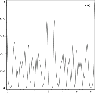
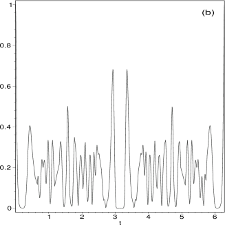
Figure 14: Squared modulus $|\langle J,0\,|\,J,\omega t\rangle|^{2}$ of the autocorrelation for the Pöschl–Teller potential with $n_{\rm max=10}$, for (a) $J=20$; (b) $J=40$.

Most interesting is the temporal behavior of the average position $\langle Q\rangle$ and of the average momentum $\langle P\rangle$ in such coherent states

$$\langle J,0\,|\,A(t)\,|\,J,0\rangle = \langle J,0\,|\,e^{\frac{i}{\hbar}Ht}Ae^{-\frac{i}{\hbar}Ht}\,|\,J,0\rangle$$ (9.23)

$$= \langle J,\omega t=\gamma\,|\,A\,|\,J,\omega t=\gamma\rangle.$$

for $A=Q$ or $A=P\equiv P_{1}$. This temporal behavior is shown in Figure 15 for the average position in the infinite square-well, for $J=2,10,50$. We note the tendency to stability around the classical mean value $\frac{1}{2}\pi a$, except for strong oscillations of ultrashort duration between the walls near $\gamma=n\pi$. The latter increase with $J$ as expected when one approaches the classical regime. For the sake of comparison, we show in Figure 16 the temporal behavior of the average position in the asymmetric Pöschl–Teller potential $(\kappa,\lambda)=(4,8)$, for $J=20$ and 50.

Figure 15: Temporal behavior of the average position of the particle in the infinite square-well (in the Heisenberg picture), $\langle J,0\,|\,Q(t)\,|\,J,0\rangle=\langle J,\omega t=\gamma\,|\,Q\,|\,J,\omega t=\gamma\rangle$, as a function of $\gamma=\omega t$, for $J=2,10,50$.

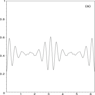
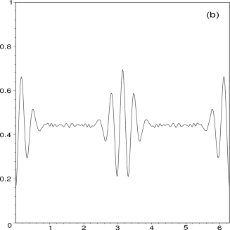
Figure 16: Temporal behavior of the average position for the asymmetric Pöschl–Teller potential $(\lambda,\kappa)=(4,8)$ with $n_{\rm max=10}$, for (a) $J=20$; and (b) $J=50$.

Figure 17: Temporal behavior of the average momentum $\langle J,0\,|\,P(t)\,|\,J,0\rangle$ in the case of the infinite square-well, for $J=2,10,50$.

Figure 17 shows the temporal behavior of the average momentum $\langle J,0\,|\,P(t)\,|\,J,0\rangle$ in the case of the infinite square-well, for $J=2,10,50$. Like in Figure 15, we note the presence of strong ultrashort oscillations at $\gamma=n\pi$, whereas a tendency to perfect stability (around the classical mean value 0) exists at intermediate values of $\gamma$ (this tendency is, however, less marked than for the average position).

Figure 18: Temporal behavior of the squared uncertainty in position $(\Delta Q)^{2}$, in the case of the infinite square-well, for $J=2,10,50$.

Figure 19: Temporal behavior of the squared uncertainty in momentum $(\Delta P)^{2}$, in the case of the infinite square-well, for $J=2,10,50$.

Next, we examine the uncertainty in position and momentum, in order to evaluate how close these CS come to saturating the uncertainty relations. Figure 18 shows the temporal behavior of the squared uncertainty in position, $(\Delta Q)^{2}$, for the infinite square-well, again for $J=2,10,50$. Figure 19 does the same for momentum, $(\Delta P)^{2}$, and Figure 20 shows the product of the two, $(\Delta Q)^{2}(\Delta P)^{2}$. We note here that the product approaches the limit value $\frac{1}{4}$ (saturation of the Heisenberg inequality) for a longer time at small $J$. This is consistent with (3.19), since at small $J$ the wave packet is centered near the ground state, for which we reach the minimal value $(0.57)^{2}$. On the other hand, we also note the strong oscillations of $(\Delta Q)^{2}(\Delta P)^{2}$ at half the revival time, a fact which is consistent with the previous figures, showing the average position and momentum. At $\frac{1}{2}t_{\rm rev}$, the quantum interferences are dominant and they enforce the spreading of the wave packet for a relatively long duration.

As a last information (but not the least!), we exhibit in Figure 21 the temporal behavior of the average position $\langle J,0\,|\,Q(t)\,|\,J,0\rangle$ for the infinite square-well, for a very high value $J=10^{6}$, near $\gamma=\omega t=0$. Here the quasiclassical behavior is striking in the range of values considered for $\gamma$. These temporal oscillations are clearly governed by $T_{\rm cl}\simeq\frac{\pi}{\sqrt{J}}=3\times 10^{-3}$ and should be compared with their purely classical counterpart of Figure 3.

Figure 20: Temporal behavior of the product of the squared uncertainties $(\Delta Q)^{2}\,(\Delta P)^{2}$, in the case of the infinite square-well, for $J=2,10,50$.

Figure 21: Temporal behavior of the average position in the case of the infinite square-well, for a very high value $J=10^{6}$.

X DISCUSSION

Coherent states have many roles to play in quantum theory. Among those roles is included the Hilbert space representation that coherent states induce, which is largely kinematical in nature, and the adaption of the coherent states themselves to some particular dynamics and the possible description that ensues. To accomodate these goals, the definition of what constitutes a “set of coherent states” has been increasingly broadened over the years. Widening the scope of coherent states also widens the range of potential applications. This basic principle lies behind the developments in this paper.

The minimal definition of a set of coherent states involves continuity of labeling and a resolution of unity, and, therefore, holomorphic representations and/or definitions via groups are just a small subset of the possibilities. In the present article, we have exploited this diversity in coherent state definition to study the motion of a particle in Pöschl–Teller potentials as well as in the closely related infinite square-well potential.

The specific choices we have made for the set of coherent states are based on two additional guiding principles besides continuity and resolution of unity [16, 17]. The first of these is “temporal stability,” which in words asserts that the temporal evolution of any coherent state always remains a coherent state. The second of these, referred to as the “action identity” in [17], chooses variables for the coherent state labels that have as close a connection as possible with classical “action-angle” variables. In particular, for a single degree of freedom, the label pair $(J,\gamma)$ is used to identify the coherent state $|J,\gamma\rangle$. Temporal stability means that, under the chosen dynamics, temporal evolution proceeds according to $|J,\gamma+\omega t\rangle$, for some fixed parameter $\omega$. To ensure that $(J,\gamma)$ describes action-angle variables, it is sufficient to require that the symplectic potential induced by the coherent states themselves is of Darboux form, or specifically that

$$i\hbar\langle J,\gamma|\,d\,|J,\gamma\rangle=J\,d\gamma$$

where $d\,|J,\gamma\rangle\equiv|J+dJ,\gamma+d\gamma\rangle-|J,\gamma\rangle$. Temporal stability is what fixes the phase behavior of the coherent states, i.e., the factor $e^{-i\gamma e_{n}}$ [cf. (7.15)], while ensuring that $(J,\gamma)$ are canonical action-angle variables is what fixes the amplitude behavior of the coherent states, i.e., $1/N\sqrt{[e_{n}]!}$ [cf. (7.19) and (7.20)]. The given amplitude behavior may be arrived at by other means [21], but requiring that $J$ and $\gamma$ be canonical classical coordinates is equivalent and tends to stress the physics of the situation.

In order for coherent states to interpolate well between quantum and classical mechanics, it is necessary for values of the action $J\gg\hbar$ that the quantum motion be well approximated by the classical motion. In particular, for a classical system with closed, localized trajectories, a suitable wave packet should, if possible, remain “coherent” for a number of classical periods. For the systems under study in this paper, we have demonstrated the tendency for improved packet coherence with increasing $J$ values within the range studied. For significantly larger values of $J$, we notice that the packet coherence substantially improves. Interesting results have been obtained independently in a related study by Fox and Choi [53], who found a similar packet coherence for $10$ or more classical periods for an infinite square-well, even though they used a different amplitude prescription for their coherent states. In both works, however, the probability distribution shows a Gaussian behavior for large values of $J$, and this explains the similarity of the results.

It would appear that allowing for generalized phase and amplitude behavior in the definition of coherent states has led us closer to the idealized goal of a set of coherent states adapted to a chosen system and having a large number of properties in common with the associated classical system, despite being fully quantum in their characteristics.

Note added: After completion of the present paper, the article [54] has come to the authors’ attention. This paper studies the dependence of various coherent states on the weighting parameters $\{\rho_{n}\}$ and how they effect various correlation functions of interest regarding general systems, and particularly for the hydrogen atom. The studies reported in [54] offer a good complement to those of the present paper.

Figure Captions

Figure 1 : The infinite square-well potential.

Figure 2 : The Pöschl–Teller potential $V(x)=\frac{1}{2}V_{o}\left[{\lambda(\lambda-1)}{\cos^{-2}\frac{x}{2a}}+{\kappa(\kappa-1)}{\sin^{-2}\frac{x}{2a}}\right],$ with $a=\pi^{-1}$ and for $(\lambda,\kappa)=(4,4),(4,8),(4,16)$ (from bottom to top).

Figure 3 : The position $x(t)$ of the particle trapped in the infinite square-well of width $\pi a$, as a function of time.

Figure 4 : The velocity $\mbox{\boldmath$v$}(t)$ of the particle in the infinite square-well: periodized Haar function.

Figure 5 : The acceleration $\gamma$(t) of the particle of the particle in the infinite square-well.

Figure 6 : Phase trajectory of the particle in the infinite square-well.

Figure 7 : The position $x(t)$ of the particle in the symmetric Pöschl–Teller potential $\lambda=\kappa=2$: (a) $E=8V_{o},T=\frac{\pi}{2}$; and (b) $E=16V_{o},T=\frac{\pi}{2\sqrt{2}}$ (compare Figure 3).

Figure 8 : The velocity $\mbox{\boldmath$v$}(t)$ of the particle in the symmetric (2,2) Pöschl–Teller potential, for the same values of $E$ and $T$ as in Figure 7 (compare Figure 4).

Figure 9 : The acceleration $\gamma$$(t)$ of the particle in the symmetric (2,2) Pöschl–Teller potential, for the same values of $E$ and $T$ as in Figure 7 (compare Figure 5).

Figure 10 : Upper part of the phase trajectory of the particle the symmetric (2,2) Pöschl–Teller system, for the same values of $E$ and $T$ as in Figure 7 (compare Figure 6).

Figure 11 : (a) The weighting distribution $|c_{n}|^{2}\equiv D(n,J,\nu)$ given in (9.18) for the infinite square-well $\nu=2$ and different values of $J$. Note the almost Gaussian shape at $J=300$, centered at $n=\langle n\rangle=\sqrt{J}-\frac{\nu}{2}-\frac{1}{4}\simeq 16$, a width equal to $2\Delta n=\sqrt{2}J^{1/4}\simeq 5.9$; (b) The same for for the harmonic oscillator: $|c_{n}|^{2}=\frac{1}{n!}|\alpha|^{2n}e^{-|\alpha|^{2}}.$ The values of $\alpha$ are chosen so as to get essentially the same mean energy values as in (a): $\alpha=\sqrt{J}$.

Figure 12 : The evolution (vs. $\gamma$) of the probability density $|\langle x|J,\gamma\rangle|^{2}$, in the case of the infinite square-well for (a) $J=2$; (b) $J=10$; and (c) $J=50$. We note the perfect revival at $\gamma=\pi=\frac{1}{2}t_{\rm rev}$ (in suitable units), symmetrically with respect to the center of the well.

Figure 13 : Squared modulus $|\langle J,0\,|\,J,\omega t\rangle|^{2}$ of the autocorrelation vs. $\gamma=\omega t$ for the infinite square-well, for $J=2,10,50$. As in Figure 12, the large $J$ regime is characterized by the occurrence of fractional revivals.

Figure 14 : Squared modulus $|\langle J,0\,|\,J,\omega t\rangle|^{2}$ of the autocorrelation for the Pöschl–Teller potential with $n_{\rm max=10}$, for (a) $J=20$; (b) $J=40$..

Figure 15 : Temporal behavior of the average position of the particle in the infinite square-well (in the Heisenberg picture), $\langle J,0\,|\,Q(t)\,|\,J,0\rangle=\langle J,\omega t=\gamma\,|\,Q\,|\,J,\omega t=\gamma\rangle$, as a function of $\gamma=\omega t$, for $J=2,10,50$.

Figure 16 : Temporal behavior of the average position for the asymmetric Pöschl–Teller potential $(\lambda,\kappa)=(4,8)$ with $n_{\rm max=10}$, for (a) $J=20$; and (b) $J=50$.

Figure 17 : Temporal behavior of the average momentum $\langle J,0\,|\,P(t)\,|\,J,0\rangle$ in the case of the infinite square-well, for $J=2,10,50$.

Figure 18 : Temporal behavior of the squared uncertainty in position $(\Delta Q)^{2}$, in the case of the infinite square-well, for $J=2,10,50$.

Figure 19 : Temporal behavior of the squared uncertainty in momentum $(\Delta P)^{2}$, in the case of the infinite square-well, for $J=2,10,50$.

Figure 20 : Temporal behavior of the product of the squared uncertainties $(\Delta Q)^{2}\,(\Delta P)^{2}$, in the case of the infinite square-well, for $J=2,10,50$.

Figure 21 : Temporal behavior of the average position in the case of the infinite square-well, for a very high value $J=10^{6}$.

References

- [1]
- [2] P. W. Atkins, Physical Chemistry, 4th ed. (Oxford University Press, Oxford, 1990).
- [3] L. Landau and E. Lifshitz, Quantum Mechanics, 2nd ed. (Addison-Wesley, Reading, MA, 1965).
- [4] S. Flügge, Practical Quantum Mechanics. I (Springer-Verlag, Berlin, Heidelberg and New York, 1971).
- [5] M. Reed and B. Simon, Methods of Modern Mathematical Physics, I. Functional Analysis, II. Fourier Analysis, Self-Adjointness, IV. Analysis of Operators (Academic Press, New York, 1972, 1975, 1978).
- [6] G. Pöschl and E. Teller, “Bemerkungen zur Quantenmechanik des anharmonischen Oszillators,” Z. Physik 83, 143–151 (1933).
- [7] A. Inomata, H. Kuratsuji, and C. C. Gerry, Path Integrals and Coherent States of SU(2) and SU(1,1) (World Scientific, Singapore, 1992).
- [8] F. L Scarf, “New soluble energy band problem,” Phys. Rev. 112, 1137–1140 (1958).
- [9] H. Li and D. Kusnezov, “Group theory approach to band structure: Scarf and Lamé Hamiltonians,” Phys. Rev. Lett. 83, 1283–1286 (1999); “Dynamical symmetry approach to periodic Hamiltonians,” J. Math. Phys. 41, 2706–2722 (2000).
- [10] N. Rosen and Ph. M. Morse, “On the vibrations of polyatomic molecules,” Phys. Rev. 42, 210–217 (1932).
- [11] C. Daskaloyannis, “Generalized deformed oscillator corresponding to the modified Pöschl–Teller energy spectrum,” J. Phys. A: Math. Gen. 25, 261–272 (1992).
- [12] Y. Alhassid, F. Gürsey, and F. Iachello, “Group theory approach to scattering,” Ann. Phys.(NY) 148, 346–380 (1983); “Potential scattering, transfer matrix, and group theory,” Phys. Rev. Lett. 50, 873–876 (1983).
- [13] A. Frank and K. B. Wolf, “Lie algebras for systems with mixed spectra. I. The scattering Pöschl–Teller potential,” J. Math. Phys. 26, 973–983 (1985).
- [14] J. R. Klauder, “Continuous-representation theory. I. Postulates of continuous-representation theory, II. Generalized relation between quantum and classical dynamics,” J. Math. Phys. 4, 1055–1073 (1963).
- [15] S. T. Ali, J-P. Antoine, and J-P. Gazeau, Coherent States, Wavelets and Their Generalizations (Springer-Verlag, New York, 2000).
- [16] J. R. Klauder, “Coherent states for the hydrogen atom,” J. Phys. A: Math. Gen. 29, L293–298 (1996).
- [17] J-P. Gazeau and J. R. Klauder, “Coherent states for systems with discrete and continuous spectrum,” J. Phys. A: Math. Gen. 32, 123–132 (1999).
- [18] J-P. Gazeau and P. Monceau, “Generalized coherent states for arbitrary quantum systems,” in Conférence Moshé Flato 1999 – Quantization, Deformations, and Symmetries, edited by G. Dito and D. Sternheimer, Vol. II, pp. 131–144 (Kluwer, Dordrecht, 2000).
- [19] F. H. Jackson, “-form of Taylor’s theorem,” Messenger Math. 38, 62–64 (1909).
- [20] C. Daskaloyannis, “Generalized deformed oscillator and nonlinear algebras,” J. Phys. A: Math. Gen. 24, L789–L794 (1991); C. Daskaloyannis and K. Ypsilantis, “A deformed oscillator with Coulomb energy spectrum,” J. Phys. A: Math. Gen. 25, 4157–4166 (1992).
- [21] A.I. Solomon, “A characteristic functional for deformed photon phenomenology,” Phys. Lett. A 196, 29–34 (1994); J. Katriel and A.I. Solomon, “Nonideal lasers, nonclassical light, and deformed photon states,” Phys. Rev. A 49, 5149–5151 (1994).
- [22] J. Blank, P. Exner, and M. Havlíček, Hilbert Space Operators in Quantum Physics (AIP Press, American Institute of Physics, New York, 1994).
- [23] M. Bouziane and Ph. A. Martin, “Bogoliubov inequality for unbounded operators and the Bose gas,” J. Math. Phys. 28, 1848–1851 (1987).
- [24] G. Lassner, G. A. Lassner, and C. Trapani, “Canonical commutation relations on the interval,” J. Math. Phys. 17, 174–177 (1976).
- [25] C. Trapani, “Quasi *-algebras of operators and their applications,” Rev. Math. Phys. 7, 1303–1332 (1995).
- [26] R. Seki, “On boundary conditions for an infinite square-well potential in quantum mechanics,” Am. J. Phys. 39, 929–931 (1971).
- [27] R. W. Robinett, “Visualizing the collapse and revival of wave packets in the infinite square well using expectation values,” Am. J. Phys. 68, 410–420 (2000).
- [28] K. Gottfried, Quantum Mechanics. Vol. I: Fundamentals (Benjamin, New York and Amsterdam, 1966).
- [29] M. Goodman, “Path integral solution to the infinite square-well,” Am. J. Phys. 49, 843–847 (1981).
- [30] R. D. Richtmayer, Principles of Advanced Mathematical Physics, Vol. I (Springer-Verlag, New York, Heidelberg, Berlin, 1978).
- [31] F. Gesztesy and W. Kirsch, “One-dimensional Schrödinger operators with interactions singular on a discrete set,” J. Reine Angew. Math. 362, 28–50 (1985); F. Gesztesy, C. Macedo, and L. Streit, “An exactly solvable periodic Schrödinger operator,” J. Phys. A: Math. Gen. 18, L503–L507 (1985).
- [32] A. O. Barut and L. Girardello, “New “coherent” states associated with non compact groups,” Commun. Math. Phys. 21, 41–55 (1971).
- [33] J-P. Gazeau and B. Champagne, “The Fibonacci-deformed harmonic oscillator,” in Algebraic Methods in Physics – A Symposium for the 60th Birthday of Jiři Patera and Pavel Winternitz, edited by Y. Saint-Aubin and L. Vinet, CRM Series in Mathematical Physics (Springer-Verlag, Berlin) (to appear).
- [34] N. Ya. Vilenkin, Special Functions and the Theory of Group Representations, (Amer. Math. Soc., Providence, RI, 1968); French transl., Fonctions Spéciales et Théorie de la Représentation des Groupes (Dunod, Paris, 1969).
- [35] I. M. Gel’fand, M. I. Graev, and N. Ya. Vilenkin, Generalized Functions. Vol. 5, Integral Geometry and Representation Theory (Academic Press, New York and London, 1966); French transl., Les distributions. Tome 5 (Dunod, Paris, 1970).
- [36] A. W. Knapp, Lie Groups Beyond an Introduction (Birkhäuser-Verlag, Basel, 1996).
- [37] K. A. Penson and A. I. Solomon, “New generalized coherent states,” J. Math. Phys. 40, 2354–2363 (1999).
- [38] J-M. Sixdeniers, K. A. Penson, and A. I. Solomon, “Mittag-Leffler coherent states,” J. Phys. A: Math. Gen. 32, 7543–7563 (1999).
- [39] J-M. Sixdeniers and K. A. Penson, “On the completeness of coherent states generated by binomial distribution,” J. Phys. A: Math. Gen. 33, 2907–2916 (2000).
- [40] J. R. Klauder, K. A. Penson, and J-M. Sixdeniers, in preparation.
- [41] W. Magnus, F. Oberhettinger, and R. P. Soni, Formulas and Theorems for the Special Functions of Mathematical Physics, 3rd ed. (Springer-Verlag, Berlin, Heidelberg and New York, 1966).
- [42] M. M. Nieto and L. M. Simmons, Jr, “Coherent states for general potentials,” Phys. Rev. Lett. 41, 207–210 (1987).
- [43] D. L. Aronstein and C. R. Stroud, “Fractional wave-function revivals in the infinite square well,” Phys. Rev. A 55, 4526–4537 (1997).
- [44] I. Sh. Averbuch and N. F. Perelman, “Fractional revivals: Universality in the long-term evolution of quantum wave packets beyond the correspondence principle dynamics,” Phys. Lett. A 139, 449–453 (1989).
- [45] W. Kinzel, “Bilder elementare Quantenmechanik,” Phys. Bl. 51, 1190–1191 (1995).
- [46] R. L. Matos Filho and W. Vogel, “Nonlinear coherent states,” Phys. Rev. A 54, 4560–4563 (1996).
- [47] F. Großmann, J-M. Rost, and W. P. Schleich, “Spacetime structures in simple quantum systems, J. Phys. A: Math. Gen. 30, L277–L283 (1997).
- [48] P. Stifter, W. E. Lamb, Jr, and W. P. Schleich, “The particle in the box revisited,” in Proceedings of the Conference on Quantum Optics and Laser Physics, edited by L. Jin and Y. S. Zhu (World Scientific, Singapore, 1997)
- [49] I. Marzoli, O. M. Friesch, and W. P. Schleich, Quantum carpets and Wigner functions, in Proceedings of the 5th Wigner Symposium (Vienna,1997), edited by P. Kasperkovitz and D. Grau, pp. 323–329 (World Scientific, Singapore, 1998).
- [50] R. Bluhm, V. A. Kosteleckỳ, and J. A. Porter, “The evolution and revival structure of localized quantum wave packets,” Am. J. Phys. 64, 944–953 (1996).
- [51] L. Mandel, “Sub-Poissonian photon statistics in resonance fluorescence,” Opt. Lett. 4, 205–207 (1979).
- [52] J. Peřina, Quantum Statistics of Linear and Nonlinear Optical Phenomena, Reidel, Dordrecht, 1984
- [53] R. Fox and M. H. Choi, “Generalized coherent states and quantum-classical correspondence,” Phys. Rev. A 61, 032107, 1–11 (2000).
- [54] M. G. A. Crawford, “Temporally stable coherent states in energy-degenerate systems: The hydrogen atom,” Phys. Rev. A 62, 012104, 1–7 (2000).