Random walks on hyperbolic groups and their Riemann surfaces

Abstract

We investigate invariants for random elements of different hyperbolic groups. We provide a method, using Cayley graphs of groups, to compute the probability distribution of the minimal length of a random word, and explicitly compute the drift in different cases, including the braid group $B_{3}$. We also compute in this case the return probability. The action of these groups on the hyperbolic plane is investigated, and the distribution of a geometric invariant, the hyperbolic distance, is given. These two invariants are shown to be related by a closed formula.

I Introduction

This paper is devoted to a systematic study of random walks on the modular group $PSL(2,{\sf Z\kern-4.49997ptZ})$ and on some closely related groups: the braid group $B_{3}$, the Hecke groups $H_{q}$ and the free groups $F_{n}$ (all definitions are given below). We study simultaneously the limiting distribution of random walks on the Cayley graphs of these groups and on their Riemann surfaces. We analyze the statistical properties of random walks on the Cayley graphs of the above mentioned groups both in a metric of words and in the natural metric of the hyperbolic plane.

The very subject of our investigation is not new—the statistics of Markov chains on the subgroups of the group $PSL(2,{\sf I\kern-1.49994ptR})$ has been extensively studied in the mathematical literature. Among the known results connected to the theme of our work we can mention: (a) the central limit theorem for Markov multiplicative processes on discrete subgroups of the group $PSL(2,{\sf I\kern-1.49994ptR})$ [14, 17], (b) some particular examples of exact results for limiting distribution functions of random walks on Cayley graphs of free and modular groups [11, 24, 25, 22] and (c) conjectures concerning the return probability and drift on the braid group $B_{3}$ [6, 7].

In the present work we rigorously compute the drift and the return probability for symmetric random walks (in metric of words) on the groups $H_{q}$ and $B_{3}$. Moreover, as it has been said, we pay a special attention to the statistics of random walks on the Riemann surfaces of the groups $PSL(2,{\sf Z\kern-4.49997ptZ}),B_{3},H_{q},F_{n}$. Namely, we study a $2\times 2$ matrix representation of these groups and consider their homographic action on the hyperbolic plane ${\cal H}$. This allows to embed the Cayley graphs in ${\cal H}$, and to define isometric hyperbolic lattices. Taking advantage of the hyperbolic metric on ${\cal H}$, we investigate the probability distribution of the geodesic distance between ends of random processes with symmetric transition probabilities on these lattices of ${\cal H}$. We show that this problem reduces to the study of the modulus of a random product of matrices. The part of our investigation is semi–analytic and is based on numerical results on the structure of the invariant distribution of geodesics at the boundary of ${\cal H}$. We found very interesting the fact that the drift on a Cayley graph in a metric of words coincides after proper normalization with the drift on the corresponding isometric lattice of ${\cal H}$ in the natural hyperbolic metric. This result establishes a nontrivial relation between two group invariants: in one hand the irreducible length of an element, which does not depend on the representation, and on the other hand, the hyperbolic distance associated to an element (directly linked to its modulus), defined only for this matrix representation.

As an application of our results, we consider the relation between the distribution of Alexander knot invariants and the asymptotic behavior of random walks over the elements of the simplest nontrivial braid group $B_{3}$. This class of problems arises naturally even beyond the aims of our particular investigation: the limiting behavior of Markov chains on braid and so-called ”local” groups can be regarded as a first step in a consistent development of harmonic analysis on branched manifolds (Teichmüller spaces are an example).

The paper is structured as follows. In section II we give the basic definitions and introduce the different groups and their Cayley graphs. A general solution of the diffusion problem on these graphs, as well as exact computations of the drift and the return probability for $B_{3}$ are developed in section III. Section IV is devoted to the study of the action of these groups in the hyperbolic plane; a discussion of our results and the relation between the different approaches are presented in section V.

II Hyperbolic groups $PSL(2,{\sf Z\kern-4.49997ptZ}),\,H_{q},\,B_{3},\,F_{n}$ and their Cayley graphs

A Basic definitions

We consider a special class of so-called hyperbolic groups – the modular group $PSL(2,{\sf Z\kern-4.49997ptZ})$, and some of its generalizations – the Hecke groups $H_{q}$ and the braid group $B_{3}$. We also recall already known properties of the free groups $F_{n}$, usefull in the context of our work.

1. The modular group $PSL(2,{\sf Z\kern-4.49997ptZ})$ is a free product ${{\sf Z\kern-4.49997ptZ}}_{2}\star{{\sf Z\kern-4.49997ptZ}}_{3}$ of two cyclic groups of 2nd (generated by $a_{2}$) and 3rd (generated by $b_{3}$ ) orders. In a standard framing using generators $S$ (inversion) and $T$ (translation), the group $PSL(2,{\sf Z\kern-4.49997ptZ})$ is defined by the following relations

$$\begin{array}[]{r}(ST)^{3}=b_{3}^{3}=1\\ S^{2}=a_{2}^{2}=1\end{array}$$ (1)

Being a discrete subgroup of the group $PSL(2,{\sf I\kern-1.49994ptR})$, the generators $T$ and $S$ of the modular group $PSL(2,{\sf Z\kern-4.49997ptZ})$ have a natural representation by unimodular matrices $\hat{T}$ and $\hat{S}$:

$$\hat{T}=\left(\begin{array}[]{cc}1&1\\ 0&1\end{array}\right);\qquad\hat{S}=\left(\begin{array}[]{cc}0&1\\ -1&0\end{array}\right)$$ (2)

2. In addition to the modular group $PSL(2,{\sf Z\kern-4.49997ptZ})$ we shall consider the so-called Hecke group $H_{q}$ which “interpolates” between the modular group (for $q=3$) and the free group $F_{3}$ with 3 generators, the so-called $\Lambda$ group (for $q=\infty$). The Hecke group $H_{q}$ is isomorphic to ${{\sf Z\kern-4.49997ptZ}}_{2}\star{{\sf Z\kern-4.49997ptZ}}_{q}$ (we denote by $a_{2}$ and $b_{q}$ the generators of orders 2 and $q$). It is defined by straightforward generalization of the relations (1)

$$\begin{array}[]{r}(ST_{q})^{q}=b_{q}^{q}=1\\ S^{2}=a_{2}^{2}=1\end{array}$$ (3)

and the generators $T_{q}$ and $S$ have the following matrix representation (compare to (2)):

$$\hat{T}_{q}=\left(\begin{array}[]{cc}1&2\cos\frac{\pi}{q}\\ 0&1\end{array}\right);\qquad\hat{S}=\left(\begin{array}[]{cc}0&1\\ -1&0\end{array}\right)$$ (4)

The parameter $q$ takes the discrete values $q=3,4,5,6,\ldots$.

3. The braid group $B_{3}$ is defined by the following commutation relations among generators $\{\sigma_{1},\sigma_{2}\}$:

$$\begin{array}[]{l}\sigma_{1}\sigma_{2}\sigma_{1}=\sigma_{2}\sigma_{1}\sigma_{2}\\ \sigma_{1}\sigma_{1}^{-1}=\sigma_{2}\sigma_{2}^{-1}=e\end{array}$$ (5)

In our further construction we shall repeatedly use the following framing:

$$\begin{array}[]{l}{\tilde{a}}=\sigma_{1}\sigma_{2}\sigma_{1}\\ {\tilde{b}}=\sigma_{1}^{-1}\sigma_{2}^{-1}\end{array}$$ (6)

The generators of the group $B_{3}$ can be represented by $PGL(2,{{\sf I\kern-1.49994ptR}})$–matrices. To be more specific, the generators $\sigma_{1}$ and $\sigma_{2}$ in the Magnus representation [9] read

$$\hat{\sigma}_{1}=\left(\begin{array}[]{cc}-t&1\\ 0&1\end{array}\right);\qquad\hat{\sigma}_{2}=\left(\begin{array}[]{cc}1&0\\ t&-t\end{array}\right)$$ (7)

where $t$ is the free parameter. We conveniently introduce the parameter $u=\sqrt{-t}$, and consider normalized generators of determinant 1:

$${}_{u}\hat{\sigma}_{1}=\left(\begin{array}[]{cc}u&1/u\\ 0&1/u\end{array}\right);\qquad{}_{u}\hat{\sigma}_{2}=\left(\begin{array}[]{cc}1/u&0\\ -u&u\end{array}\right)$$ (8)

The group generated by ${}_{u}\hat{\sigma}_{1}$ and ${}_{u}\hat{\sigma}_{2}$ will be denoted later on as $PSL(2,{\sf Z\kern-4.49997ptZ})_{u}$. Indeed it is just a deformation of $PSL(2,{\sf Z\kern-4.49997ptZ})$, which preserves all its commutation relations. For $u=1$, one has $PSL(2,{\sf Z\kern-4.49997ptZ})_{u}=PSL(2,{\sf Z\kern-4.49997ptZ})$, and the group $B_{3}$ is a central extension of $PSL(2,{\sf Z\kern-4.49997ptZ})_{u}$ of center

$$(\hat{\sigma}_{1}\hat{\sigma}_{2})^{3\lambda}=(\hat{\sigma}_{2}\hat{\sigma}_{1})^{3\lambda}=(\hat{\sigma}_{1}\hat{\sigma}_{2}\hat{\sigma}_{1})^{2\lambda}=(\hat{\sigma}_{2}\hat{\sigma}_{1}\hat{\sigma}_{2})^{2\lambda}=\left(\begin{array}[]{cc}t^{3\lambda}&0\\ 0&t^{3\lambda}\end{array}\right),\ \forall\lambda\in{\sf Z\kern-4.49997ptZ}$$ (9)

(let us note that the center is isomorphic to ${\sf Z\kern-4.49997ptZ}$). Recall that graphically, to each word of $B_{3}$ correspond a particular three–strand braid, going from above downwards. (see Fig.1). A closed braid is obtained by gluing the ”top” and ”bottom” free ends on a cylinder. Any closed braid defines a link (in particular, a knot). However the correspondence between braids and knots (links) is not one–to–one and each link (knot) can be represented by infinite number of different braids (see [8, 9]). The irreducible length of a braid gives nevertheless an interesting characteristic of the link complexity.

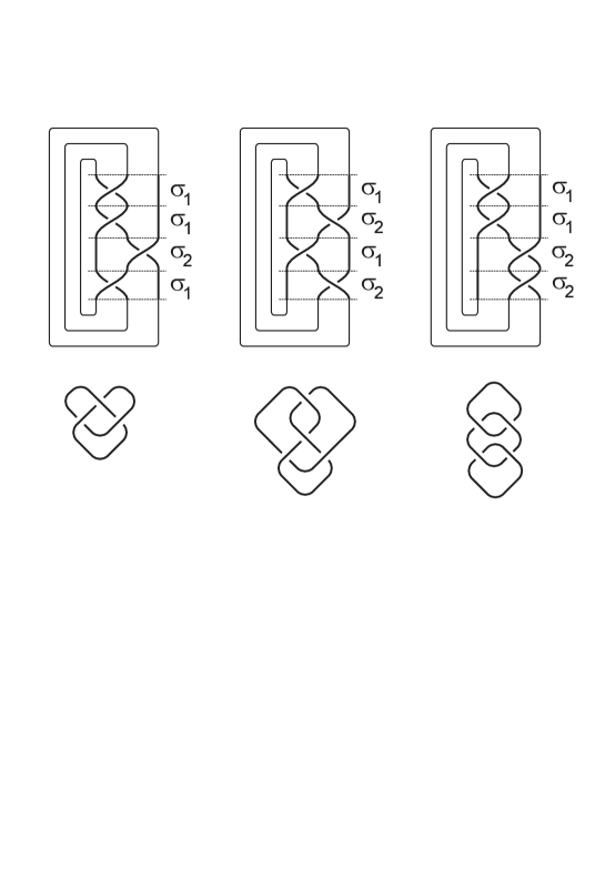
FIG. 1.: Some examples of closed braids and corresponding links.

There exists an extensive literature on general properties of braid groups—see [9]; for the last works on the normal forms of words, we shall quote [10].

Any element of the group $G=\{PSL(2,{\sf Z\kern-4.49997ptZ}),H_{q},B_{3}\}$ is defined by a word in alphabets of corresponding letters (generators):

• $\{S,T,T^{-1}\}$ or $\{a_{2},b_{3},b_{3}^{-1}\}$—for $PSL(2,{\sf Z\kern-4.49997ptZ})$

• $\{S,T_{q},T_{q}^{-1}\}$ or $\{a_{2},b_{q},b_{q}^{-1}\}$—for $H_{q}$

• $\{\sigma_{1},\sigma_{2},\sigma_{1}^{-1},\sigma_{2}^{-1}\}$ or $\{\tilde{a},\tilde{a}^{-1},\tilde{b},\tilde{b}^{-1}\}$—for $B_{3}$.

We denote by $w_{n}$ a word corresponding to a given record of length $n$, and by $L^{G}(w_{n})$ the irreducible length in the metric of words (the superscript $G$ is precised only when it is necessary), or in other terms the minimal number of generators necessary to build $w_{n}$. The irreducible length can be also viewed as a distance from the unity on the Cayley graph of the group $G$. Note that $L^{G}(w)$ depends on the set of generators we consider.

B Cayley graphs

The modular group $PSL(2,{\sf Z\kern-4.49997ptZ})$ is a particular case of the Hecke group $H_{q}$ at $q=3$. We therefore consider without any loss of generality the Cayley graphs of the groups $H_{q}$ for $q=3,4,...$. The Cayley graph of $B_{3}$ will be constructed afterwards. We investigate in this part only the abstract presentation of the groups in terms of commutation relations and do not pay attention to any representation. We recall that the Cayley graph of a group $G$ is the graph whose vertices are labeled by group elements, and whose links are as follows: $w$ and $w^{\prime}$ are linked if and only if there exists a generator $g$ such that $w^{\prime}=wg$. Following this rule, we can easily construct the Cayley graph ${\cal G}_{q}$ of the group $H_{q}$ represented by $\{a_{2},b_{q},b_{q}^{-1}\}$. For any finite values of $q$ the graph ${\cal G}_{q}$ has local $q$–cycles (because $b_{q}$ is of order $q$), while the corresponding dual (or ”backbone”) graph is the tree graph ${\sf T\kern-4.49997ptT}_{q}$, which is precisely the graph of $F_{q}$. This is due to the free product structure of $H_{q}\sim{\sf Z\kern-4.49997ptZ}_{2}\star{\sf Z\kern-4.49997ptZ}_{q}$ (see explanations below). The graph ${\cal G}_{q}$ is shown in Fig.2, where the backbone graph is marked by a dotted line.

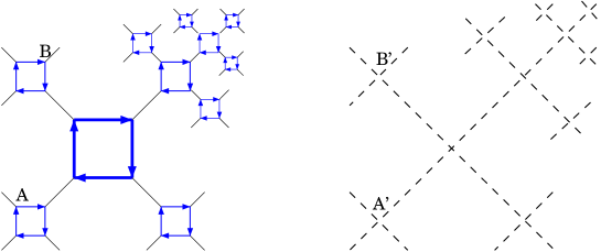
FIG. 2.: Cayley graph of $H_{q}$, with $q=4$. Arrows correspond to generator $b_{q}=ST_{q}$, thin lines to generator $a_{2}=S=S^{-1}$. The dashed graph is the corresponding backbone graph, a tree ${\sf T\kern-4.49997ptT}_{q}$, graph of $F_{q}$. The distance $d$ between A and B is $d=5$, while the distance $k$ (corresponding to the distance between A’ and B’) is $k=2$.

III Diffusion on graphs

In this section we investigate some statistical properties of random walks on the groups introduced above, using their Cayley graphs. In particular we consider simple random walks, that are walks of nearest neighbour type with symmetric transition probabilities.

A Random walk on $PSL(2,{\sf Z\kern-4.49997ptZ})$ and $H_{q}$

We consider free product groups of the form ${\sf Z\kern-4.49997ptZ}_{2}\star{\sf Z\kern-4.49997ptZ}_{q}$ (isomorphic to $H_{q}$), in the framing which uses the generators $a_{2}$ and $b_{q}$, of order $2$ and $q$ respectively. Graphs of such groups are shown in Fig.2. We define two different “metrics” of words on those graphs. The first metric is associated with the geodesic distance $d$ on the graph—the minimal number of steps between two points, and the second metric is associated with the geodesic distance $k$ (called later the ”generation”) on the backbone graph ${\sf T\kern-4.49997ptT}_{q}$. Our goal is to compute the probability $P_{q}(d,n)$ of being at a distance $d$ from the initial point (the root of the graph) after $n$ random steps. The probability ${\bar{P}}_{q}(k,n)$ of being on the backbone graph at a generation $k$ from a root point after $n$ random steps will also be of use.

First of all we compute $P_{3}(d,n)$ and ${\bar{P}}_{3}(k,n)$ for the case of $PSL(2,{\sf Z\kern-4.49997ptZ})$. In this case the graph structure ensures the relation

$$P_{3}(2x,n)={\bar{P}}_{3}(x,n)$$

Therefore we can consider only ${\bar{P}}_{3}(k,n)$. Write

$${\bar{P}}_{3}(k,n)={\bar{P}}_{3}^{i}(k,n)+{\bar{P}}_{3}^{o}(k,n)$$

distinguishing for an elementary triangular cell located at generation $k$ the vertex closest to the root (corresponding to ${\bar{P}}_{3}^{i}(k,n)$) and the two others (corresponding to ${\bar{P}}_{3}^{o}(k,n)$) (see Fig.7). A direct enumeration gives the following master equation for $k\geq 2$:

$$\left\{\begin{array}[]{l}{\bar{P}}_{3}^{i}(k,n+1)=\frac{1}{3}\left({\bar{P}}_{3}^{o}(k,n)+{\bar{P}}_{3}^{o}(k-1,n)\right)\\ {\bar{P}}_{3}^{o}(k,n+1)=\frac{2}{3}{\bar{P}}_{3}^{i}(k,n)+\frac{1}{3}\left({\bar{P}}_{3}^{o}(k,n)+{\bar{P}}_{3}^{i}(k+1,n)\right)\end{array}\right.$$ (10)

with initial conditions of the form

$$\left\{\begin{array}[]{l}{\bar{P}}_{3}^{i}(k,0)=\alpha\delta_{k,0}\\ {\bar{P}}_{3}^{o}(k,0)=(1-\alpha)\delta_{k,0}\end{array}\right.$$ (11)

where $\alpha$ is an arbitrary parameter fixing the initial condition and varying in the interval $0\leq\alpha\leq 1$. We are seeking for the asymptotic ($1\ll k\leq n$) solution to (10) near the maximum of the probability distribution, and therefore will not take into account the specific form of the boundary condition.

Define the Laplace–Fourier transform:

$$Q^{i,o}(x,s)={\cal T}\left[{\bar{P}}_{3}^{i,o}\right]=\sum_{n=0}^{\infty}s^{n}\sum_{k=-\infty}^{+\infty}e^{ikx}{\bar{P}}_{3}^{i,o}(k,n)$$ (12)

whose inverse can be written in the form

$${\bar{P}}_{3}^{i,o}(k,n)=\frac{1}{4i\pi^{2}}\oint\frac{ds}{s^{n+1}}\int_{-\pi}^{\pi}e^{-ikx}Q^{i,o}(x,s)dx$$ (13)

One straightforwardly obtains the following algebraic system of linear equations:

$$\left\{\begin{array}[]{l}\displaystyle Q^{i}(x,s)-\frac{s}{3}(1+e^{ix})Q^{o}(x,s)=\alpha\\ \displaystyle-\frac{s}{3}(2+e^{-ix})Q^{i}(x,s)+(1-\frac{s}{3})Q^{o}(x,s)=1-\alpha\end{array}\right.$$ (14)

which determines the function $Q^{i,o}(x,s)$:

$$Q^{i,o}(x,s)=\frac{a_{\alpha}^{i,o}(x)+b_{\alpha}^{i,o}(x)s}{\displaystyle s^{2}+\frac{3}{3+e^{-ix}+2e^{ix}}s-\frac{9}{3+e^{-ix}+2e^{ix}}}=\frac{a_{\alpha}^{i,o}(x)+b_{\alpha}^{i,o}(x)s}{p(x,s)}$$ (15)

where

$$\left\{\begin{array}[]{l}\displaystyle a_{\alpha}^{i}(x)=\frac{9\alpha}{3+e^{-ix}+2e^{ix}}\vskip 6.0pt plus 2.0pt minus 2.0pt\\ \displaystyle a_{\alpha}^{o}(x)=\frac{9(1-\alpha)}{3+e^{-ix}+2e^{ix}}\vskip 6.0pt plus 2.0pt minus 2.0pt\\ \displaystyle b_{\alpha}^{i}(x)=\frac{3(1-2\alpha+(1-\alpha)e^{ix})}{3+e^{-ix}+2e^{ix}}\vskip 6.0pt plus 2.0pt minus 2.0pt\\ \displaystyle b_{\alpha}^{o}(x)=\frac{3\alpha(2+e^{-ix})}{3+e^{-ix}+2e^{ix}}\end{array}\right.$$ (16)

Denote by $s_{\pm}(x)$ the roots of $p(x,s)$. Using (13) one can rewrite

$${\bar{P}}_{3}^{i,o}(k,n)=\frac{1}{2\pi}\int_{-\pi}^{\pi}dx\frac{e^{-ikx}}{s_{+}-s_{-}}\left[a_{\alpha}^{i,o}(x)\left(\frac{1}{s_{+}^{n+1}}-\frac{1}{s_{-}^{n+1}}\right)+b_{\alpha}^{i,o}(x)\left(\frac{1}{s_{+}^{n}}-\frac{1}{s_{-}^{n}}\right)\right]$$ (17)

We are interested in the $n,k\gg 1$ regime, and therefore consider the integrand in (17) for $x\to 0$. Here we expose the second order computation, keeping in mind that any order can be reached the same way. With

$$\left\{\begin{array}[]{l}\displaystyle s_{+}=-\frac{3}{2}+\frac{3ix}{20}-\frac{51x^{2}}{250}+O(x^{3})\vskip 6.0pt plus 2.0pt minus 2.0pt\\ \displaystyle s_{-}=1-\frac{ix}{15}+\frac{209x^{2}}{2250}+O(x^{3})\end{array}\right.$$ (18)

one gets

$$\begin{array}[]{lll}\displaystyle{\bar{P}}_{3}(k,n)=\frac{1}{2\pi}\int_{-\pi}^{\pi}dx\;e^{-ikx}(1-\frac{ix}{15}+\frac{209x^{2}}{2250})^{-n}&\approx&\displaystyle\frac{1}{2\pi}\int_{-\infty}^{\infty}dx\;\exp\left[-ikx-n\left(\frac{107x^{2}}{1125}-\frac{ix}{15}\right)\right]\vskip 6.0pt plus 2.0pt minus 2.0pt\\ &\approx&\displaystyle\frac{A}{n^{1/2}}\exp\left[-\frac{1125(k-\frac{n}{15})^{2}}{428n}\right]\end{array}$$ (19)

where $A$ is the normalization constant.

The expression (19) allows one to compute the limiting value of the normalized drift $\bar{l}_{3}$

$$\bar{l}_{3}=\lim_{n\to\infty}\frac{\left<k\right>_{3}}{n}$$

on the backbone graph ${\sf T\kern-4.49997ptT}_{3}$, where

$$\left<k\right>_{3}=\int_{-\infty}^{\infty}k\bar{P}_{3}(k,n)dk=\frac{n}{15}$$

and, hence, the drift $l_{3}$

$$l_{3}=\lim_{n\to\infty}\frac{\left<d\right>_{3}}{n}=2\bar{l}_{3}=\frac{2}{15}$$

on the graph $H_{3}$.

Let us generalize these computations to the case of $H_{q}$. One can write

$${\bar{P}}_{q}(k,n)=\sum_{i=1}^{[\frac{q}{2}]+1}{\bar{P}}_{q}^{i}(k,n)$$ (20)

and define the constants $\rho_{i},\ 1\leq i\leq[\frac{q}{2}]+1$ (assuming the existence of corresponding limits):

$$\rho_{i}=\lim_{k\to\infty}\left(\lim_{n\to\infty}\frac{{\bar{P}}_{q}^{i}(k,n)}{{\bar{P}}_{q}(k,n)}\right)$$ (21)

which satisfy the normalization condition

$$\sum_{i=1}^{[\frac{q}{2}]+1}\rho_{i}=1$$ (22)

FIG. 3.: Different types of vertices and their corresponding weights (here $q=6$). $\rho_{i}$ gives the asymptotic ($k,n\to\infty$) probability of being at a vertex of type $i$.

The sum (20) runs over $[\frac{q}{2}]+1$ non-equivalent vertices (the graph is locally ${\sf Z\kern-4.49997ptZ}_{2}$ symmetric, see Fig.3) of the elementary $q$–gone of the graph. Proceeding in the standard way, we define the transform

$$Q^{i}_{q}(x,s)={\cal T}\left[{\bar{P}}_{q}^{i}\right]$$ (23)

and derive the master equation, whose solution can be expressed in the following form

$${\bar{P}}_{q}^{i}={\cal T}^{-1}\left[\sum_{j=1}^{n_{q}}\alpha_{j}(M_{q}^{-1})^{ji}(x,s,\vec{\rho})\right]$$ (24)

where the $\alpha_{j}$ parametrize the initial conditions

$$\sum_{i=1}^{[\frac{q}{2}]+1}Q_{q}^{i}M_{q}^{ij}(x,s,\vec{\rho})=\alpha_{j}$$ (25)

and

$$M_{q}(x,s,\vec{\rho})=\displaystyle\pmatrix{-1&\frac{s}{3}(1+e^{ix})&\frac{s}{3}e^{ix}&\cdots&\cdots&\frac{s}{3}e^{ix}\cr\frac{s}{3}(2+\frac{\rho_{2}}{1-\rho_{1}}e^{-ix})&-1&\frac{s}{3}&0&\cdots&0\cr\frac{s}{3}\frac{\rho_{3}}{1-\rho_{1}}e^{-ix}&\frac{s}{3}&-1&\frac{s}{3}&\ddots&\vdots\cr\frac{s}{3}\frac{\rho_{4}}{1-\rho_{1}}e^{-ix}&0&\ddots&\ddots&\ddots&0\cr\vdots&\vdots&\ddots&\frac{s}{3}&-1&\frac{s}{3}\cr\frac{s}{3}\frac{\rho_{n}}{1-\rho_{1}}e^{-ix}&0&\cdots&0&\frac{s}{3}&-1+\frac{s}{3}\cr}$$ (26)

For $n,k\gg 1$ one obtains, using the same method as for $q=3$

$${\bar{P}}_{q}^{i}(k,n)={\bar{\rho}}_{i}(\vec{\rho})\delta(k-{\bar{l}}_{q}(\vec{\rho})n)$$ (27)

where

$${\bar{l}}_{q}(\vec{\rho})=\lim_{n\to\infty}\frac{\langle k\rangle_{q}}{n}=i\frac{ds^{q}_{-}}{dx}$$ (28)

and $s^{q}_{-}$ is the root of the polynomial ${\rm det}\left(M_{q}(x,s,\vec{\rho})\right)$ the closest to zero.

To make the system of equations (24)–(26) self–consistent we must set

$$\rho_{i}={\bar{\rho}}_{i}(\vec{\rho})$$ (29)

which closes a system of equations determining $\rho_{i}$. Finally, one can write the limiting drift in the following form

$$l_{q}=\lim_{n\to\infty}\frac{\left<d\right>_{q}}{n}={\bar{l}}_{q}(\vec{\rho})\left(1+\frac{\sum_{i=2}^{n_{q}}(i-1)\rho_{i}}{1-\rho_{1}}\right)$$ (30)

One can check that this formalism gives for $q=3$ the same results as has been derived above.

B Random walk on $B_{3}$: drift and return probability

1 Analytic results

We now focus on the braid group $B_{3}$ and in particular explain why some statistical characteristics of random processes on $B_{3}$ have the same asymptotic behavior as the ones on $PSL(2,{\sf Z\kern-4.49997ptZ})$. The key point is that $B_{3}$ is a central extension of $PSL(2,{\sf Z\kern-4.49997ptZ})$. Let us recall that the center $Z$ of $B_{3}$, generated by ${\tilde{a}}^{2}={\tilde{b}}^{3}=\Delta^{2}$, is isomorphic to ${\sf Z\kern-4.49997ptZ}$. We denote by $\pi$ the canonical quotient map

$$\pi:\ B_{3}\longrightarrow\frac{B_{3}}{Z}\sim PSL(2,{\sf Z\kern-4.49997ptZ})$$ (31)

One has then

$$\left\{\begin{array}[]{l}\pi(\sigma_{1})={\bar{\sigma}}_{1}=a_{2}b_{3}\\ \pi(\sigma_{2})={\bar{\sigma}}_{2}=b_{3}a_{2}\\ \pi({\tilde{a}})=a_{2}\\ \pi({\tilde{b}})=b_{3}\end{array}\right.$$ (32)

where $a_{2}$ and $b_{3}$ are defined in (1)

A natural representation of the Cayley graph of $B_{3}$ is three dimensional. As shown in Fig.4, the map $\pi$ can then be viewed as a projection from 3D to 2D.

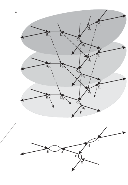
FIG. 4.: $B_{3}$ Cayley graph and its projection ($PSL(2,{\sf Z\kern-4.49997ptZ})$). Thin arrows correspond to ${\tilde{a}}$, thick ones to ${\tilde{b}}$. Note that $\pi(\alpha_{i})=\alpha$, $\pi(\beta_{i})=\beta$ and so on. Recall that $a_{2}$ has to be identified with $a^{-1}_{2}$

Consider now an $n$–letter random word $w_{n}$ written in terms of generators of the group $B_{3}$:

$$w_{n}=\prod_{i=1}^{n}\sigma_{r_{i}}$$

where we set $\sigma^{-1}_{r_{i}}=\sigma_{-r_{i}}$ and indices $r_{i}$ are uniformly distributed in $\{-2,-1,1,2\}$. We recall that $L^{B_{3}}(w_{n})$ is the irreducible length of $w_{n}$. It is evident that

$$L^{B_{3}}(w_{n})\geq L^{PSL(2,{\sf Z\kern-3.14998ptZ})}(\pi(w_{n}))$$ (33)

(keeping in mind the geometrical interpretation of $B_{3}$ shown in Fig.4, we can easily derive eq.(33) following from a triangular inequality). Consider now the irreducible decomposition in $PSL(2,{\sf Z\kern-4.49997ptZ})$:

$$\pi(w_{n})=\prod_{i=1}^{L^{PSL(2,{\sf Z\kern-2.24998ptZ})}(\pi(w_{n}))}{\bar{\sigma}}_{r^{\prime}_{i}}$$ (34)

The asymptotic value of $\left<L^{PSL(2,{\sf Z\kern-3.14998ptZ})}(\pi(w_{n}))\right>$ for $n\gg 1$ is computed in appendix A by a straightforward adaptation of the method introduced in a previous section. From (34) and the definition of the quotient map, we get:

$$w_{n}={\Delta}^{2f(n)}\prod_{i=1}^{L^{PSL(2,{\sf Z\kern-2.24998ptZ})}(\pi(w_{n}))}\sigma_{r^{\prime}_{i}}$$ (35)

where $\Delta^{2}$ is 6–letter word in the alphabet $\{\sigma_{1},...,\sigma_{2}^{-1}\}$ (see Eq.9), what implies the following condition on $f(n)$:

$$|f(n)|\leq\frac{n}{6}$$

Hence, the irreducible length of the word $w_{n}$ can be estimated from above

$$L^{B_{3}}(w_{n})\leq 6|f(n)|+L^{PSL(2,{\sf Z\kern-3.14998ptZ})}(\pi(w_{n}))$$ (36)

Let us show now that the Markovian process $f(n)$ is such that

$$\left<|f(n)|\right>=O(\sqrt{n})$$ (37)

1. The symmetry of the process implies that the words $\Delta^{2}$ and ${\Delta}^{-2}$ appear with same probability, which gives $\left<f(n)\right>=0$.

2. The increment $|f(n+1)-f(n)|$ is bounded from above by some constant.

Thus, the central limit theorem gives (37). This, together with (33) and (36) allows one to write

$$\frac{L^{PSL(2,{\sf Z\kern-3.14998ptZ})}(\pi(w_{n}))}{n}\leq\frac{L^{B_{3}}(w_{n})}{n}\leq\frac{L^{PSL(2,{\sf Z\kern-3.14998ptZ})}(\pi(w_{n}))}{n}+O\left(\frac{1}{\sqrt{n}}\right)$$ (38)

Using the result $\lim_{n\to\infty}L^{PSL(2,{\sf Z\kern-3.14998ptZ})}(\pi(w_{n}))/n=1/4$ obtained in Appendix for symmetric random walk on $PSL(2,{\sf Z\kern-4.49997ptZ})$ one arrives at the following asymptotic expression

$$l_{B_{3}}=\lim_{n\to\infty}\frac{L^{B_{3}}(w_{n})}{n}=\frac{1}{4}$$ (39)

2 Statistics of loops on $B_{3}$: return probability for ”magnetic” random walks

The investigation carried out above shows that if a random walk on the group $B_{3}$ ends in $Z(B_{3})$ (we will say in this case a $Z$–walk), it can be regarded as a closed ”magnetic” random walk on $PSL(2,{\sf Z\kern-4.49997ptZ})$. Namely, if one inserts in each elementary cell of the hyperbolic lattice a ”magnetic flux” $h$ (see Fig.4) and denotes by $\Phi$ the total flux through a closed path on $PSL(2,{\sf Z\kern-4.49997ptZ})$, then any word $w^{Z}_{n}$ corresponding to a $Z$–walk on $B_{3}$ can be written as

$$w^{Z}_{n}={\Delta}^{2\Phi/h}$$

In other words, the group $B_{3}$ being the central extension of $PSL(2,{\sf Z\kern-4.49997ptZ})$, gives rise to a fibre bundle above $PSL(2,{\sf Z\kern-4.49997ptZ})$ such that every full turn around the elementary cell leads to another sheet of the Riemann surface of $PSL(2,{\sf Z\kern-4.49997ptZ})$. The outcome of this construction is that $Z$–walks on $B_{3}$ can be decomposed into a product of elementary full turns around cells (this is due to the tree structure of the backbone). Hence the function $u_{n}(\Phi)$ giving the probability that a closed $n$–step loop on a graph $PSL(2,{\sf Z\kern-4.49997ptZ})$ carries a flux $\Phi$ is of great interest, especially because at $\Phi=0$ it defines the probability to get a trivial braid (i.e. completely reducible word) from a random braid of the record length $n$.

First of all we compute $u^{a}_{n}(\Phi)$ for a walk with local passages in a basis $\{a_{2},b_{3},a_{2}^{-1},b_{3}^{-1}\}$ (let us stress that for magnetic walks $a_{2}\not=a_{2}^{-1}$). Denote by $\sharp a_{2},\sharp a_{2}^{-1},\sharp b_{3},\sharp b_{3}^{-1}$ the total number of steps $a_{2},a_{2}^{-1},b_{3},b_{3}^{-1}$ respectively in a given closed path on $PSL(2,{\sf Z\kern-4.49997ptZ})$. The fulx $\Phi$ can be written as follows:

$$\Phi=\frac{h}{6}\left(3(\sharp a_{2}-\sharp a_{2}^{-1})+2(\sharp b_{3}-\sharp b_{3}^{-1})\right)$$ (40)

Recall that we consider an $n$–step process on $PSL(2,{\sf Z\kern-4.49997ptZ})$, conditioned by the fact that the path is closed (i.e. returns to the origin). Following (40), we rise a simultaneous process $\Phi_{i}$ (with $\Phi_{0}=0$) such that

$$\Phi_{i+1}=\Phi_{i}+\phi_{i+1}$$ (41)

with $\phi_{i}=\pm h/2$ if the corresponding step on $PSL(2,{\sf Z\kern-4.49997ptZ})$ is $a_{2}^{\pm 1}$, or $\phi_{i}=\pm h/3$ if the step is $b_{3}^{\pm 1}$. Evidently the final value $\Phi_{n}$ gives the total flux $\Phi$ through the closed path.

We show that the process $\Phi_{i}$ is not affected by the condition that the path is closed.

1. Notice that on $PSL(2,{\sf Z\kern-4.49997ptZ})$ we have $a_{2}^{-1}=a_{2}$, and therefore $p(h/2)=p(-h/2)$.

2. The sign of the magnetic field can be arbitrarily changed, hence $p(h/3)=p(-h/3)$ (i.e. positive, $b_{3}^{3}$, and negative, $b_{3}^{-3}$, elementary turns are equidistributed for closed as well as for open paths).

3. The closure condition on $PSL(2,{\sf Z\kern-4.49997ptZ})$ affects the irreducible length of words; the irreducible forms on $PSL(2,{\sf Z\kern-4.49997ptZ})$ being exactly the words of the form $a^{\pm 1}b^{\pm 1}a^{\pm 1}b^{\pm 1}a^{\pm 1}...$, setting the irreducible length of a word does not change the relative weight of $a^{\pm 1}$ and $b^{\pm 1}$ in this word. One finally obtains $p(h/2)=p(h/3)$.

The process $\Phi_{i}$ is then a classical one dimensional random walk, and therefore for $n$ large one has

$$u^{a}_{n}(\Phi)=\frac{1}{h\sigma_{a}\sqrt{2\pi n}}\exp\left(-\frac{(\Phi/h)^{2}}{2n\sigma_{a}^{2}}\right)$$ (42)

where $\sigma_{a}^{2}=\frac{1}{2}\left(\frac{1}{4}+\frac{1}{9}\right)=\frac{13}{72}$.

This result seems to be interesting in the context of lattice random walks in a transversal magnetic field which has relations to the Harper–Hofstadter problem (see [12] for review) in hyperbolic geometry.

Returning to the random walk on the braid group in the standard framing $\{\sigma_{1},\sigma_{2},\sigma_{1}^{-1},\sigma_{2}^{-1}\}$, we can compute the distribution $u^{\sigma}_{n}(\Phi)$ for a random process on $\{{\bar{\sigma}}_{1},{\bar{\sigma}}_{2},{\bar{\sigma}}_{1}^{-1},{\bar{\sigma}}_{2}^{-1}\}$. Modifying slightly the derivation carried out above, one obtains that the corresponding process $\phi_{i}$ is still not affected by the condition of return, and is such that $p(\phi_{i}=h/6)=p(\phi_{i}=-h/6)=1/2$. This yields

$$u^{\sigma}_{n}(\Phi)=\frac{1}{h\sigma_{\sigma}\sqrt{2\pi n}}\exp\left(-\frac{(\Phi/h)^{2}}{2n\sigma_{\sigma}^{2}}\right)$$ (43)

with $\sigma_{\sigma}^{2}=\frac{1}{36}$.

The decomposition introduced above allows to compute the return probability, i.e the probability $p(w_{n}=I_{d})=p_{r}(n)$ to obtain a “trivial” braid after $n$ random elementary moves. Using (35) the condition $w_{n}=I_{d}$ is equivalent to the conditions

$$L^{PSL(2,{\sf Z\kern-3.14998ptZ})}(\pi(w_{n}))=0\;\&\;f(n)=0$$

Denote

$$p\{L^{PSL(2,{\sf Z\kern-3.14998ptZ})}(\pi(w_{n}))=0\}=p^{\pi}_{r}(n)$$

and

$$p\{f(n)=0\ {\rm knowing}\ L^{PSL(2,{\sf Z\kern-3.14998ptZ})}(\pi(w_{n}))=0\}=p^{c}_{r}(n)$$

The probabilities $p^{\pi}_{r}(n)$ and $p^{c}_{r}(n)$ are independent which allows us to set

$$p_{r}(n)=p^{\pi}_{r}(n)p^{c}_{r}(n)$$ (44)

where $p^{\pi}_{r}(n)$ is computed in appendix A and $p^{c}_{r}(n)$ can be reexpressed the following way

$$p^{c}_{r}(n)=hu^{\sigma}_{n}(0)$$ (45)

Collecting (44)–(45) we arrive at the final expression for $p_{r}(n)$

$$p_{r}(n)=\frac{C}{\sigma_{\sigma}\sqrt{2\pi}}\frac{{\lambda}^{n}}{n^{2}}$$ (46)

where $\lambda$ and $C$ are given in appendix.

3 Numerical results

So far there is no constructive algorithm to find the reduced form of words of $B_{3}$ for generators $\sigma_{i}$. The existence of an algorithm depends crucialy on the set of generators we choose. Indeed, it is shown in [5] that computing the length in terms of generators $\sigma_{i}$ of a braid in $B_{n}$ is an NP–complete problem. Let us mention nevertheless that braid groups are “biautomatic” (see [4]) which basically means that there exists a set of generators, for which the reduced words are exactly known. This allows in particular to solve the word enumeration problem, and to implement methods which can compare two different braids in a polynomial time (see [3]). In our case of the simplest nontrivial group $B_{3}$ we tried a random reduction procedure, but it converges only in exponential time. Since our analytical results are obtained in the regime $(n\gg 1)$, the numerical simulations give no additionnal information.

IV Diffusion on Riemann surfaces: traces and Lyapunov exponents

We consider the representation of dimension 2 of the groups introduced above, and investigate their action on the hyperbolic Poincaré plane ${\cal H}=\{z,\ {\rm Im}\,z>0\}$. Namely, we consider the following fractional-linear transforms

$$\left(\begin{array}[]{cc}a&b\\ c&d\end{array}\right):\ z\to\frac{az+b}{cz+d}$$ (47)

We recall that $PSL(2,{\sf I\kern-1.49994ptR})$ is a subgroup of the group of isometries of ${\cal H}$. The groups $PSL(2,{\sf Z\kern-4.49997ptZ}),PSL(2,{\sf Z\kern-4.49997ptZ})_{u},H_{q},F_{n}$ admit representations as subgroups of $PSL(2,{\sf I\kern-1.49994ptR})$ and their Cayley graphs (considered in previous section) are now viewed as isometric lattices embedded into ${\cal H}$. Now one can investigate their metric properties using the natural hyperbolic (geodesic) distance in ${\cal H}$. We define the lattices under consideration the same way as we have defined the Cayley graphs:

• We construct the set of all possible orbits of a given root point (we choose the point $i=(0,1)$ for conveniency) under the action of the group.

• We denote by $d(w_{n})$ the hyperbolic distance $d(i,w_{n}(i))$ between $i$ and $w_{n}(i)$.

• We call ”lattices” the Cayley graphs of the groups involved here because of two important features:

  • they are discrete subgroups of $PSL(2,{\sf I\kern-1.49994ptR})$, the group of motion of the hyperbolic 2-space. Hyperbolic distance is a pair–point invariant, that is $d(i,w(i))=d(\gamma i,w\gamma(i))$, what jusities the term isometric;

  • they have the property of so-called lattice groups: they have no points of accumulation (for the topology of ${\cal H}$). Recall that for $H_{q}$, $q\in{\sf Z\kern-4.49997ptZ}$.

Let us add that the above description is based on well known results on Fuchsian groups theory (see [15, 14]). Properties of a Fuchsian group $G$ depend strongly on the fundamental domain of $G$, which is a minimal set of points generating ${\cal H}$ under action of $G$. The groups studied throughout this paper are all Fuchsian groups. We first remind that the fundamental domain of the Hecke group is the circular triangle with angles $\left\{0,\frac{\pi}{q},\frac{\pi}{q}\right\}$ (see Fig.5 for $H_{3}$).

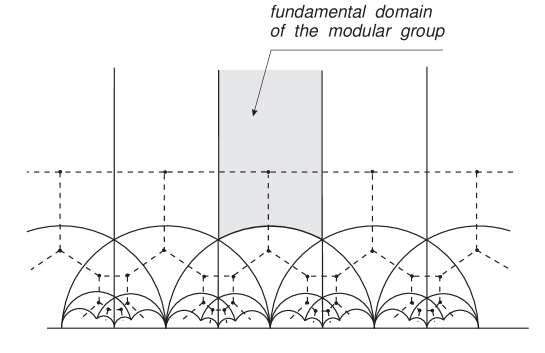
FIG. 5.: Fundamental domain of $PSL(2,{\sf Z\kern-4.49997ptZ})$

It can be shown that the fundamental domain of $F_{n}$ is a zero-angled n-gone. Our contribution to this subject concerns the construction of the fundamental domain of the deformed group $PSL(2,{\sf Z\kern-4.49997ptZ})_{u}$ (Fig.6).

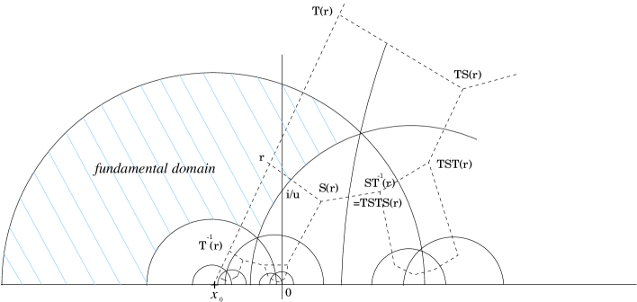
FIG. 6.: Fundamental domain of $PSL(2,{\sf Z\kern-4.49997ptZ})_{u}$, for $u=1.2$.

We omit technical details of this construction, which can be found in [14]. The outline is as follows. We first find the fixed point $i/u$ of $S_{u}$, and $x_{0}=1/(1-u^{2})$ of $T_{u}$. We then draw the only geodesic through $i/u$ which intersects its images by $T_{u}$ and $T_{u}^{-1}$ with angle $\pi/3$. Circles of center $x_{0}$ passing by these intersections complete the construction. First notice that the topology of the Cayley graph obtained this way does not depend on $u$. Recall that only commutation relations, independent of $u$, set the topological structure of the Cayley graph). Only the metric properties are affected by $u$. In particular the area of the fundamental domain is finite only for $u=1$. The group is then said to be of type I in the classification of Fuchsians groups. For $u\not=1$ it is of type II. It means that the corresponding monodromy problems are deeply different (see [16]). Solving the monodromy problem is an important issue since it allows to get the conformal transform that maps the fundamental domain onto ${\cal H}$. To our knowledge the problem is solved only for $u=1$. We have therefore to content ourselves with an existence theorem in the general case. Existence of such a transform allows to define a map $f_{u}$ from the fundamental domain of $PSL(2,{\sf Z\kern-4.49997ptZ})_{u}$ to the fundamental domain of $PSL(2,{\sf Z\kern-4.49997ptZ})$. The action of $PSL(2,{\sf Z\kern-4.49997ptZ})_{u}$ on ${\cal H}$ is in this sense conjugate to the action of $PSL(2,{\sf Z\kern-4.49997ptZ})$:

$$\forall\omega_{u}\in PSL(2,{\sf Z\kern-4.49997ptZ})_{u},\ \omega_{u}(z)=f_{u}^{-1}\circ\omega_{u=1}\circ f_{u}(z)$$ (48)

The dependence on the parameter $u$ is this way clearly expressed.

A Analytic results

Let us return to the definition of the model and recall that the groups under consideration act in the hyperbolic Poincaré upper half–plane ${\cal H}=\{z\in\kern 1.00006pt{\raise 2.0236pt\hbox{$\scriptscriptstyle|$}}\kern-3.99994pt{\sf C},\,{\rm Im}(z)>0\}$ by fractional–linear transforms. The matrix representation of the generators (denoted by $h_{i}$, $1\leq i\leq n_{g}$) of the different groups has been given in section II.

Choosing the point $(x_{0},y_{0})=(0,i)$ as the tree root—see fig.5, we associate any vertex on the lattice with an element $\displaystyle w_{n}=\prod_{k=1}^{n}h_{\alpha_{k}}$ where $1\leq\alpha_{k}\leq n_{g}$ and $w_{n}$ is parametrized by its complex coordinates $z_{n}=w_{n}\big{(}i\big{)}$ in the hyperbolic plane.

Strictly speaking ${\cal H}$ should be identified with $SL(2,{\sf I\kern-1.49994ptR})/SO(2)$; we here identify an element with its class of equivalence of $SO(2)$. The following identity holds (see [14, 18])

$$2\cosh\Big{(}d(w_{n})\Big{)}={\rm Tr}(w_{n}w_{n}^{{\dagger}})$$ (49)

where dagger denotes transposition.

We are interested in the distribution function $P_{n}(d)$, and therefore have to look for the distribution of traces of matrices $w_{n}$. The method described hereafter involves mainly the results of the paper [13]. The outline of our approach is as follows. We study the behavior of the random matrix $w_{n}$, generated by a Markov chain (which must fulfill ergodicity properties) defined as follows:

$$w_{n+1}=M_{n}h_{\alpha_{n+1}}{\rm,}\ (\alpha_{n+1}=i,\ 1\leq i\leq n_{g})\ {\rm with\ probability}\ \frac{1}{n_{g}}$$ (50)

We use the standard methods of random matrices and consider the entries of the $2\times 2$–matrix $w_{n}$ as a 4–vector ${\cal V}_{n}$. The transformation $w_{n+1}=w_{n}h_{\alpha}$ reads now

$${\cal V}_{n+1}=\left(\begin{array}[]{ll}h_{\alpha}^{{\dagger}}&0\\ 0&h_{\alpha}^{{\dagger}}\end{array}\right)\;{\cal V}_{n}$$ (51)

This block–diagonal form allows to study one of two 2–vectors composing ${\cal V}_{n}$, say $v_{n}$. Parametrizing $v_{n}=(\varrho_{n}\cos\theta_{n},\varrho_{n}\sin\theta_{n})$ and using the relation $d(w_{n})\equiv d_{n}\simeq 2\ln\varrho_{n}$ valid for $n\gg 1$, one gets a recursion relation $v_{n+1}=h_{\alpha}^{{\dagger}}v_{n}$ in terms of hyperbolic distance $d_{n}$:

$$d_{n+1}=d_{n}+\ln\,p_{\alpha}(\cos\theta)$$ (52)

where $p_{\alpha}$ is a second order polynomial depending on the specific form of transition matrices $h_{\alpha}$. While for the angles one gets straightforwardly

$$\cot\theta_{n+1}=h_{\alpha}\left(\cot\theta_{n}\right)$$ (53)

The action of $h_{\alpha}$ is fractional–linear.

One has now to study the invariant measure $\mu(\theta)$, giving the asymptotic probability to have $\theta_{n}=\theta$. Introducing $x=\cot\theta$, we are led to study the action of the group restricted on the real line parametrized by $x$. The statistical properties of $\mu$ have been discussed by Gutzwiller and Mandelbrot [1] in the case of the free group $\Lambda$. An alternative, put forward in [13], is to define $\mu(x)$ as the limit of the following recursion relation:

$$\mu^{(n+1)}(x)=\frac{1}{n_{g}}\sum_{\alpha=1}^{n_{g}}\mu^{(n)}\Big{(}h_{\alpha}(x)\Big{)}\left|\frac{dh_{\alpha}(x)}{dx}\right|$$ (54)

The convergence $\mu^{(n)}(x)\to\mu(x)$ for $n\to\infty$ is assured by ergodic properties of the functional transform (54) and has been successfully checked numerically by comparing to direct sampling of different orbits. Despite the absence of rigorous proof, we claim that $\mu$ is defined with no ambiguity by (54). This enables us to compute the desired distribution $P_{n}(d)$. The crucial point required for convergence of $\mu^{(n)}$ to the invariant distribution, is the existence of ergodic properties of $\theta_{n}$. It means that for $n\gg 1$, the distribution of $\theta_{n}$ is exactly given by $\mu(\theta)$, independently of $n$ and initial conditions. We introduce the generating function for (52); due to the Markovian structure of (52), we can perform the averaging:

$$\left<e^{ikd_{n+1}}\right>=\left<e^{ikd_{n}}\right>\left<[p_{\alpha}(\cos\theta)]^{ik}\right>$$ (55)

Thus we obtain

$$\left<e^{ikd_{n}}\right>=\left[\frac{1}{n_{g}}\sum_{\alpha=1}^{n_{g}}\int_{-\pi/2}^{\pi/2}d\theta\mu(\theta)[p_{\alpha}(\cos\theta)]^{ik}\right]^{n}$$ (56)

This form suggests that for $n$ large $P_{n}(d)$ satisfies a central limit theorem. Indeed such a theorem exists (see [17, 20]) for Markovian processes provided that the phase space is ergodic. We are then led to compute only the first two moments (Lyapunov exponents), which gives us

$$\gamma_{1}=\lim_{n\to\infty}\frac{\left<d\right>}{n}=\frac{1}{n_{g}}\sum_{\alpha=1}^{n_{g}}\int_{-\pi/2}^{\pi/2}d\theta\mu(\theta)\ln p_{\alpha}(\cos\theta)$$ (57)

and

$$\sigma^{2}=\lim_{n\to\infty}\frac{\left<(d-\left<d\right>)^{2}\right>}{n}=\gamma_{2}-\gamma_{1}^{2}$$ (58)

where

$$\gamma_{2}=\frac{1}{n_{g}}\sum_{\alpha=1}^{n_{g}}\int_{-\pi/2}^{\pi/2}d\theta\mu(\theta)\ln^{2}p_{\alpha}(\cos\theta)$$ (59)

B Numerical results

We present in this part the numerical and semi-analytical results for the invariant measure $\mu$ and the Lyapounov exponent $\gamma_{1}$. Our main goal is to compare the approach developed here with the results following from the study of random walks on graphs (see section III.

Let us call the backbone subgroup ${\cal B}(G)$ of the group $G$ such subgroup of $G$ whose Cayley graph is the backbone of the graph of $G$. It seems to be more instructive to rely on this purely geometrical caracterization of ${\cal B}$ and to avoid a formal formal definition. Let us stress that ${\cal B}(G)$ is a free subgroup of $G$. One has for example ${\cal B}(F_{n})=F_{n}$. Consider now the representation of $F_{q}$ by $q$ idempotent generators $g_{1},..,g_{q}$ with the following homomorphism $\Psi$:

$$\Psi:\left\{\begin{array}[]{lll}F_{q}&\longrightarrow&H_{q}\\ g_{i}&\longrightarrow&b_{q}^{-i}a_{2}b_{q}^{i}\end{array}\right.$$ (60)

Due to injectivity of $\Psi$, the following decomposition holds

$$H_{q}=\bigcup_{i=1}^{q}b_{q}^{i}\Psi(F_{q})$$ (61)

with

$$b_{q}^{i}\Psi(F_{q})\bigcap b_{q}^{j}\Psi(F_{q})=\emptyset\ {\rm for}\ i\not=j$$ (62)

what means that the Cayley graph of $H_{q}$ is the disjoint union of $q$ trees ${\sf T\kern-4.49997ptT}_{q}$. Thus we set ${\cal B}(H_{q})=F_{q}$.

The scale factor $s_{f}$ is the “average” irreducible length of the generators of ${\cal B}(G)$ in $G$. In other words, $L^{G}(w)\sim s_{f}L^{{\cal B}(G)}(w)$ for $w\in{\cal B}(G)$ with $L^{G}(w)\gg 1$. We have studied two different Markovian processes for each group $G$: (i) simple random walks (characterized by the Lyapunov exponent $\gamma_{1}^{s}$) and (ii) so-called directed random walks (that are walks excluding two consecutive opposite steps) on the backbone subgroup ${\cal B}(G)$ (caracterized by Lyapunov exponent $\gamma_{1}^{d}$).

By construction $\gamma_{1}^{d}/s_{f}$ gives the average hyperbolic length for an elementary step on $G$. We conjecture that $s_{f}\gamma_{1}^{s}/\gamma_{1}^{d}$ gives the number of steps to the origin (normalized by $n$) on the graph $G$. Let us point out that this result links together two definitions of the ”drift” for random walks on the groups $G$: the drift $l$ is defined on the graph in metric of words while $\gamma$ is defined in terms of hyperbolic distance for an isometric embedding of $G$ into ${\cal H}$. Thus we claim

$$\left<L^{G}(w)\right>=\frac{s_{f}}{\gamma_{1}^{d}}\left<\ln{\rm Tr}(ww^{{\dagger}})\right>$$ (63)

where a word $w$ is identified with its matrix representation. We believe that equation 63 is worth interest, since it relates properties of a group defined only trough symbolic commutation relations, to geometrical properties of a given representation.

The stochastic average $\left<...\right>$ in (63) is necessary, to wash out purely geometrical effects such as multifractality investigated in [13]. (It corresponds to fluctuations of the hyperbolic distance for words of same length on the backbone graph). One has to stress that (63) holds due to a “global” spherical symmetry (see [26] for a precise definition of this symmetry for graphs) of both models; only the “radial” part of the processes is considered, whereas the angular dependence is averaged (here again the ergodic properties play the crucial role). This has been checked numerically in the continuous case: generators have to be properly normalized, such that each elementary step should have the same hyperbolic length, ensuring spherical symmetry, else the invariant measure $\mu$ fails to converge.

All results are summarized in table I.

group	generators	${\mbox{backbone subgroup},\atop\mbox{scale factor $s_{f}$}}$	${s_{f}\gamma_{1}^{s}/\gamma_{1}^{d}\atop\mbox{numerical}}$	${s_{f}\gamma_{1}^{s}/\gamma_{1}^{d}\atop\mbox{semi--analytical}}$	${\left<d\right>/n:\atop\mbox{graph approach}}$
$F_{3}$	$h_{1},h_{2},h_{3}$	$F_{3},\ 1$	0.3334	0.332	1/3
$F_{4}$	$h_{1},h_{2},h_{1}^{-1},h_{2}^{-1}$	$F_{4},\ 1$	0.501	0.503	1/2
$H_{3}$	$a_{2},b_{3},b_{3}^{-1}$	$F_{3}$, 2	0.1334	0.132	$2/15=0.133..$
$PSL(2,{\sf Z\kern-4.49997ptZ})$	$\bar{\sigma}_{1},\bar{\sigma}_{2},\bar{\sigma}_{1}^{-1},\bar{\sigma}_{2}^{-1}$	$F_{3}$, 1	0.2501	0.248	$1/4$

TABLE I.:

V Discussion and perspectives

We have presented during this work different aspects of random walks on a family of hyperbolic groups. On one hand we studied the Cayley graphs of these groups, and briefly exposed general methods of computing the Green functions for Markovian processes on those graphs; in particular we explicitly calculate the drift in different cases. As an application, we studied Markovian processes on the braid group $B_{3}$, and explicitly showed that the drift for a symmetric random walk on this group tends at $n\to\infty$ to the drift of a process on the group $PSL(2,{\sf Z\kern-4.49997ptZ})$, which is found to be $1/4$. This means that a typical random braid of record length $n$ can be released on average by $n/4$ elementary moves. The graph approach and the introduction of “magnetic walks” enabled us also to compute explicitely the return probability on $B_{3}$, that is the probability to obtain a trivial (completely reducible) braid from a random word of record length $n$.

On the other hand we took advantage of the fact that the groups $H_{q}$ and $PSL(2,{\sf Z\kern-4.49997ptZ})_{u}$ are subgroups of $PSL(2,{\sf I\kern-1.49994ptR})$ and therefore act naturally in the hyperbolic plane $\cal H$. The Cayley graphs of these groups are then naturally embedded in $\cal H$. Instead of the usual length in metric of word, we could, thanks to this representation, use the metric structure of $\cal H$ and study the hyperbolic length of random elements of the group. This problem leads to the study of products of random matrices. The method described in [13] allows us to compute the probability distribution of the hyperbolic length. Lyapunov exponents are explicitely computed in different cases.

These two approaches are shown to be related by an equation (63). This result is a strong motivation for investigating further the geometric properties of hyperbolic groups in connexion with other topological invariants. As an example we briefly mention the Alexander polynomials.

The Alexander polynomial $\nabla_{K}(t)$ of a link $K$ represented by a closed braid $w_{n}=\prod_{j=1}^{n}\sigma_{r_{j}}$ of length $n$ is defined as follows

$$(1+t+t^{2})\,\nabla_{K}(t)=\det\left[\prod_{j=1}^{n}\hat{\sigma}_{r_{j}}-\hat{I}\right]=\det\left[\prod_{j=1}^{n}\hat{\sigma}_{r_{j}}\right]+1-{\rm Tr}\left[\prod_{j=1}^{n}\hat{\sigma}_{r_{j}}\right]$$ (64)

where $j$ runs “along the braid”, i.e. labels the number of used generators, the subscript $r_{j}\in\{-2,-1,1,2\}$ marks the set of braid generators (letters), with the prescription $\hat{\sigma_{i}}^{-1}=\hat{\sigma}_{-i}$ and $\hat{I}$ defines the $2\times 2$–identity matrix. For long words ($n\gg 1$), the following asymptotic expression holds:

$${\rm Tr}(w_{n})\sim\left({\rm Tr}(w_{n}w_{n}^{{\dagger}})\right)^{1/2}\sim e^{d(w_{n})/2}$$ (65)

One then has, with the parameter $u=\sqrt{-t}$ (recall that $\hat{\sigma_{i}}$ depends on $u$):

$$(1-u^{2}+u^{4})\,\nabla_{K}(u)=u^{2p(w_{n})}-u^{p(w_{n})}e^{d(w_{n})/2}+1$$ (66)

with $p(w_{n})=\sharp(+)-\sharp(-)$. In this regime the polynomial is therefore expressed only in terms of $p(w_{n})$ and $d(w_{n})$. The quantity $p(w_{n})$ is a “poor” invariant, in sense that it takes the same value for a large amount of links. In other words $p(w_{n})$ is just the length of the element $w_{n}$ projected onto ${\sf Z\kern-4.49997ptZ}$. Indeed there exists an obvious group homomorphism $\pi_{1}$ from $B_{3}$ to ${\sf Z\kern-4.49997ptZ}$ defined by $\pi_{1}(\sigma_{i}^{\pm 1})=\pm 1$. All non abelian properties are lost by this invariant. The geometric invariant $d(w_{n})$, described above, is much stronger. As we have shown, this invariant is related directly to the word length in the group $PSL(2,{\sf Z\kern-4.49997ptZ})$, which preserves the noncommutative structure of $B_{3}$ (recall that the random word length in $B_{3}$ has the same asymptotics as the word length in $PSL(2,{\sf Z\kern-4.49997ptZ})$). The information is nevertheless not redundant, because there is no nontrivial homorphism from $PSL(2,{\sf Z\kern-4.49997ptZ})$ to ${\sf Z\kern-4.49997ptZ}$ (there is no finite order element in ${\sf Z\kern-4.49997ptZ}$). In particular, under the condition $d(w_{n})=0$ (Z–walks), $p$ is an exact invariant having sense of a winding number.

The form (66) seems in particular convenient for possible problems of statistics of Alexander polynomials, since we know the statistics of both $p$ and $d$. In particular, for a simple random walk, the typical Alexander polynomial could be defined as ${\bar{\nabla}}_{n}(u)$:

$$(1-u^{2}+u^{4}){\bar{\nabla}}_{n}(u)=1-e^{n\gamma_{1}(u)/2}$$ (67)

where $\gamma_{1}(u)$ is the Lyapunov exponent of the random product of generators $\hat{\sigma}_{i}$.

A Drift on $PSL(2,{\sf Z\kern-4.49997ptZ})$

The goal of this appendix is to compute the drift of a random walk on $PSL(2,{\sf Z\kern-4.49997ptZ})$ in terms of generators $\bar{\sigma}_{i}$. We keep notations of III and proceed the same way, noting that the process under consideration is no longer a simple random walk, but is described by the transitions shown in fig.7.

FIG. 7.: Random walk on $PSL(2,{\sf Z\kern-4.49997ptZ})$ in terms of generators $\bar{\sigma}_{i}$. Vertices of type i and o are shown.

A direct counting gives the following master equation for $k\geq 2$:

$$\left\{\begin{array}[]{l}{\bar{P}}_{3}^{i}(k,n+1)=\frac{1}{4}\left({\bar{P}}_{3}^{i}(k+1,n)+2{\bar{P}}_{3}^{i}(k-1,n)+{\bar{P}}_{3}^{o}(k-1,n)\right)\vskip 6.0pt plus 2.0pt minus 2.0pt\\ {\bar{P}}_{3}^{o}(k,n+1)=\frac{1}{4}\left({\bar{P}}_{3}^{o}(k+1,n)+{\bar{P}}_{3}^{i}(k+1,n)+2{\bar{P}}_{3}^{o}(k-1,n)\right)\end{array}\right.$$ (A1)

with initial conditions of the form

$$\left\{\begin{array}[]{l}{\bar{P}}_{3}^{i}(k,0)=\alpha\delta_{k,0}\vskip 6.0pt plus 2.0pt minus 2.0pt\\ {\bar{P}}_{3}^{o}(k,0)=(1-\alpha)\delta_{k,0}\end{array}\right.$$ (A2)

One then straightforwardly obtains the following algebraic linear system:

$$\left\{\begin{array}[]{l}\displaystyle Q^{i}(x,s)\left(1-\frac{s}{4}(e^{-ix}+2e^{ix})\right)-\frac{s}{4}e^{ix}Q^{o}(x,s)=\alpha\vskip 6.0pt plus 2.0pt minus 2.0pt\\ \displaystyle-\frac{s}{4}e^{-ix}Q^{i}(x,s)+\left(1-\frac{s}{4}(e^{-ix}+2e^{ix})\right)Q^{o}(x,s)=1-\alpha\end{array}\right.$$ (A3)

determining $Q^{i,o}(x,s)$:

$$Q^{i,o}(x,s)=\frac{a_{\alpha}^{i,o}(x)+b_{\alpha}^{i,o}(x)s}{p(x,s)}$$ (A4)

We omit the details irrelevant for the purpose of this Appendix. We denote as $s_{\pm}(x)$ the roots of $p(x,s)$. They obey the equations

$$\left\{\begin{array}[]{l}\displaystyle s_{+}=2-ix+O(x^{2})\vskip 6.0pt plus 2.0pt minus 2.0pt\\ \displaystyle s_{-}=1-\frac{ix}{4}+O(x^{2})\end{array}\right.$$ (A5)

and one gets finally

$$\frac{\langle k\rangle_{3}}{n}=\frac{1}{4}$$ (A6)

One has now to make sure that for any word $w_{n}$ of $n$ letters in the alphabet ${\bar{\sigma}_{i}}$ the following relation holds:

$$k(w_{n})=L(w_{n})+O(1)$$ (A7)

Even if Fig.7 makes this statement clear, a more rigorous proof is as follows. Consider a given word $w$, with $k(w)=k_{0}$. Then the following decomposition holds:

$$w=b_{3}^{\epsilon_{0}}\left(\prod_{i=1}^{k_{0}}a_{2}b_{3}^{\epsilon_{i}}\right)a_{2}^{\epsilon_{f}}$$ (A8)

with $\epsilon_{0}\in\{0,1,2\},\ \epsilon_{i}\in\{1,2\},\ \epsilon_{f}\in\{0,1\}$. To prove (A7) we use the relation

$$L\left(\prod_{i=1}^{k_{0}}a_{2}b_{3}^{\epsilon_{i}}\right)=k_{0}$$ (A9)

and one has finally

$$\lim_{n\to\infty}\frac{L(w_{n})}{n}=\frac{1}{4}$$ (A10)

Let us mention that a more direct derivation of this result can be brought in if one considers the $PSL(2,{\sf Z\kern-4.49997ptZ})$ generators . The structure of the Cayley graph of $PSL(2,{\sf Z\kern-4.49997ptZ})$ depends on the basis and in the framing $S,T,T^{-1}$ it has form of the so-called hyperbolic honeycomb lattice (see Fig.8).

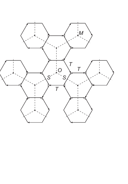
FIG. 8.: The honey-comb lattice.

Define $\kappa$—the distance on the backbone graph of $PSL(2,{\sf Z\kern-4.49997ptZ})$. The partition function $P_{n}(\kappa)$ to find the random walker at a distance in $\kappa$ steps along the backbone graph from the origin after $n$ elementary steps satisfies the master equation:

$$P_{n+1}(\kappa)=\frac{1}{4}P_{n}(\kappa+1)+\frac{1}{4}P_{n}(\kappa)+\frac{1}{2}P_{n}(\kappa-1)$$ (A11)

with the following boundary conditions:

$$P_{n+1}(0)=\frac{1}{2}(P_{n}(0)+P_{n}(1))$$ (A12)

This is a standard problem whose solution is known, and the condition $L(w_{n})=0$ is in particular equivalent to $\kappa=0$, therefore the probability to obtain a trivial word after $n$ random steps (denoted $p^{\pi}_{r}(n)$) is given by

$$p^{\pi}_{r}(n)=P_{n}(0)=C\frac{{\lambda}^{n}}{n^{3/2}}$$ (A13)

with

$$C=\frac{9+4\sqrt{2}}{7\pi}\ \mbox{and}\ \lambda=\frac{2\sqrt{2}+1}{4}$$

REFERENCES

- [1] M. Gutzwiller, B. Mandelbrot, Phys. Rev. Lett. 60, 673 (1988)
- [2] C. Series, J. London Math. Soc. (2) 31, 69 (1985)
- [3] P. Dehornoy, Advances in math. 125, 200-235 (1997)
- [4] R. Charney, Math. Ann. 301, 307-324 (1995)
- [5] M.S. Paterson, A.A. Razborov, J. Algorithms 12, 393-408 (1991)
- [6] A.M.Vershik,S.Nechaev,R.Bibkov, Commun.Math.Phys. 212, 469–501 (2000)
- [7] S.Nechaev, A.Grosberg, A.Vershik, J.Phys.A, 29, 2411 (1996)
- [8] L.H.Kauffman, On knots, (Ann. Math. Studies 115, Princeton Univ. Press, 1987)
- [9] J.Birman, Knots, Links and Mapping Class Groups (Ann. Math. Studies 82, Princeton Univ. Press, 1976)
- [10] J.Birman, K.Ko, J.Lee, Adv. Math., 139, 322 (1999)
- [11] R. Voituriez, S. Nechaev, J. Phys. A, 33, 5631 (2000)
- [12] D.R.Hofstadter, Phys. Rev. B, 14, 2239 (1976)
- [13] A.Comtet, S.Nechaev, R.Voituriez, J. Stat. Phys., 102, 1/2 (2001)
- [14] A. Terras, Harmonic Analysis on symmetric spaces and applications I (Springer, New York, 1985)
- [15] S. Katok, Fuchsians Groups (Chicago Lectures in Mathematics,1992)
- [16] H.Bateman, Higher Transcendental Functions (McGraw–Hill, 1955)
- [17] J.L. Doob, Stochastic Processes (Wiley publications in statistics, 1953)
- [18] J.Elstrodt, F.Grunewald, J.Mennicke, Groups acting on hyperbolic space (Springer, 1998)
- [19] M. Sheingorn, Illinois J. Math. 24, 3 (1980)
- [20] P. Bougerol, Probab. Th. Rel. Fields 78, 193 (1988)
- [21] Ya.Pesin, H.Weiss, Chaos, 7, 89 (1997)
- [22] S.Nechaev, A.N.Semenov, M.K.Koleva, Physica A, 140, 506 (1987)
- [23] H.Kesten, Trans.Am.Math.Soc., 92, 336 (1959)
- [24] P.Gerl, W.Woess, Prob.Theor.Rel.Fields, 71, 341 (1986)
- [25] W.Woess, Bull.London Math.Soc., 26, (1994)
- [26] R.Lyons, Ann.Prob., 20, 125 (1992)