July 13, 2001

Quantum lattice models at intermediate temperature

J. Fröhlich¹, L. Rey-Bellet², D. Ueltschi³

¹ETH, Zürich, Switzerland
²University of Virginia, USA
³Princeton University, New Jersey, USA

Abstract. We analyze the free energy and construct the Gibbs-KMS states for a class of quantum lattice systems, at low temperature and when the interactions are almost diagonal, in a suitable basis. The models we study may have continuous symmetries, our results however apply to intermediate temperatures where discrete symmetries are broken but continuous symmetries are not. Our results are based on quantum Pirogov-Sinai theory and a combination of high and low temperature expansions.

Keywords: Pirogov-Sinai theory, phase diagrams, Gibbs phase rule, low temperature Gibbs-KMS states, quantum restricted ensembles.

Dedicated to Joel Lebowitz on the occasion of his seventieth birthday.

1. Introduction

In this paper we study the low temperature phase diagram for a class of quantum lattice systems. Starting with [PS, Sin], Pirogov-Sinai theory has evolved [KP, Zah, BKL, BS, BI, BK] into a very powerful tool to study the pure phases, their coexistence and the first-order phase transitions in classical spin systems at low temperature. In recent years large part of the Pirogov-Sinai theory has been extended to quantum systems [Pir, BKU, DFF, DFFR, KU], quantum spin systems as well as fermionic and bosonic lattice gases, and applied to a variety of models [FR, DFF2, GKU] to describe insulating phases associated with discrete symmetry breaking. Here we formulate the Pirogov-Sinai theory in terms of tangent functionals to the free energy. This allows to discuss the completeness of the phase diagram avoiding the difficulties associated with boundary conditions. We reformulate results of [BKU, DFF, DFFR, KU] in this framework, and extend the theory to a class of models where discrete symmetries are broken at intermediate temperatures. This applies in particular to some systems with continuous symmetries. For this, we consider the restricted ensembles introduced in [BKL] that are very useful to analyze phases which are associated to a family of configurations rather than to a single configuration.

The models that we consider have Hamiltonians, for finite volumes $\Lambda$, of the form

$$H_{\Lambda}\,=\,V_{\Lambda}+T_{\Lambda}$$

where $V_{\Lambda}$ is a classical Hamiltonian (i.e. diagonal in a suitable basis) and $T_{\Lambda}$ is a (usually small) quantum perturbation. In typical situations the suitable basis is the basis of occupation numbers of position operators. Electronic systems provide a large class of interesting models. The classical interaction $V_{\Lambda}$ describes the many-body short range and classical interaction between the spin-$\frac{1}{2}$ fermions as well as external fields and chemical potentials:

$$V_{\Lambda}\,=\,\ \sum_{\begin{subarray}{c}x\in\Lambda\\ \sigma\in\{\uparrow,\downarrow\}\end{subarray}}J_{x,\sigma}n_{x,\sigma}+\sum_{\begin{subarray}{c}x,y\in\Lambda\\ \sigma,\sigma^{\prime}\in\{\uparrow,\downarrow\}\end{subarray}}J_{xy,\sigma\sigma^{\prime}}n_{x,\sigma}n_{y,\sigma^{\prime}}+\cdots\,.$$

A typical quantum perturbation $T_{\Lambda}$ is the kinetic energy

$$T_{\Lambda}\,=\,\sum_{\begin{subarray}{c}<\!x,y\!>\subset\Lambda\\ \sigma\in\{\uparrow,\downarrow\}\end{subarray}}t_{xy,\sigma}(c^{\dagger}_{x\sigma}c_{y\sigma}+{\rm h.c.})\,,$$

where $c^{\dagger}_{x\sigma}$ and $c_{x\sigma}$ are the creation and annihilation operators and $<\!x,y\!>$ denotes pairs of nearest neighbors.

Often, in such systems, the behavior at low temperatures arises from a subtle interplay between the (classical) potential energy and the kinetic energy. In this paper two such mechanisms are considered and combined, each of which we now illustrate with an example.

Example 1: Hubbard Model. In this case the (classical) interaction is only on-site:

$$V_{\Lambda}\,=\,\sum_{x\in\Lambda}Un_{x\uparrow}n_{x\downarrow}-\mu(n_{x\uparrow}+n_{x\downarrow})\,.$$

For suitable values of $U$ and $\mu$, the ground states of $V_{\Lambda}$ have an infinite degeneracy (in the thermodynamic limit): each site is occupied by a single particle of arbitrary spin. However the kinetic energy lifts this degeneracy and induces an effective antiferromagnetic interaction between nearest neighbors. The perturbative methods of [DFFR, DFF2] shows that, in this parameter range, this system is equivalent, in the sense of statistical mechanics, to the Heisenberg antiferromagnet, up to controlled error terms. If the hopping coefficients are asymmetric (e.g. $t_{xy,\uparrow}\ll t_{xy,\downarrow}$) then quantum Pirogov-Sinai implies the coexistence of two antiferromagnetic phases at low enough temperatures [DFFR, KU, DFF2]. Rigorous results for the Hubbard model are reviewed in [Lieb].

Example 2: Extended Hubbard Model. This variant of the Hubbard model includes a nearest neighbor interaction:

$$V_{\Lambda}\,=\,\sum_{x\in\Lambda}\Bigl{[}Un_{x\uparrow}n_{x\downarrow}-\mu(n_{x\uparrow}+n_{x\downarrow})\Bigr{]}+W\sum_{<\!x,y\!>\subset\Lambda}(n_{x\uparrow}+n_{x\downarrow})(n_{y\uparrow}+n_{y\downarrow})\,.$$

If the the interaction between nearest neighbors is repulsive then for suitable values of $U$, $W$ and $\mu$ the ground states of $V_{\Lambda}$ are chessboard configurations where empty sites alternate with sites occupied with one particle of arbitrary spin. The degeneracy of the ground states is infinite in the thermodynamic limit but we have a spatial ordering of the particle. Using restricted ensemble we associate a pure phase to this spatial ordering by neglecting the spin degrees of freedom. The methods of this paper imply the existence of only two pure phases in the intermediate temperature range

$$\beta t\ll 1\quad{\rm~{}and~{}}\quad\beta W\gg 1\,.$$

The temperature is so low that the spatial ordering of the particles survives but so high that the spin are in a disordered phase. The continuous symmetry (if $t_{xy,\uparrow}=t_{xy,\downarrow}$) is not broken in this parameter regime.

These two models illustrate some of the mechanisms arising from the competition between classical and quantum effects, where the system remains insulating and no continuous symmetry is broken. Our main result, Theorem 4.4, provides tools to describe the phase diagram of such models, in particular the coexistence of several phases and the associated first-order phase transitions.

The main technical ingredient in this paper is a combined low-temperature and high-temperature expansion for suitable contour models obtained using the perturbation theory developed in [DFFR].

This paper is organized as follows. In Section 2 we describe the general formalism of quantum lattice systems and the perturbation theory of [DFFR]. Section 3 is devoted to the Pirogov-Sinai theory. In Section 4 we state the results of Pirogov-Sinai theory for quantum systems. The extended Hubbard model is discussed in Section 5 as an illustration. In Section 6 we prove our main result by studying a contour model and deriving the required bounds on the contours.

2. General framework of quantum lattice models

2.1. Basic set-up

We consider a quantum mechanical system on a $\nu$-dimensional lattice ${\mathbb{Z}}^{\nu}$, as considered, e.g., in [Rue, Isr, BR, Sim]. We will need a slight modification of the usual formalism in order to treat fermionic lattice gases [DFFR] and to accommodate the fact that fermionic creation and annihilation operators do not commute but anticommute. A quantum lattice system is defined by the following data:

(i) Hilbert space. For convenience we choose a total ordering (denoted by the symbol $\preceq$) of the sites in ${\mathbb{Z}}^{\nu}$. We choose the spiral order, depicted in Figure 1 for $\nu=2$, and an analogous ordering for ${\nu}\geq 3$. This ordering has the property that, for any finite set $A$, the set $\overline{A}:=\{z\in{\mathbb{Z}}^{\nu},z\preceq A\}$ of lattice sites which are smaller than $A$, or belong to $A$, is finite. To each lattice site $a\in\,{\mathbb{Z}}^{\nu}$ is associated a finite-dimensional Hilbert space ${\mathcal{H}}_{a}$ and, for any finite subset $A=\{a_{1}\prec\cdots\prec a_{n}\}\subset{\mathbb{Z}}^{\nu}$, the corresponding Hilbert space ${\mathcal{H}}_{A}$ is given by the ordered tensor product

$${\mathcal{H}}_{A}\,=\,{\mathcal{H}}_{a_{1}}\otimes\cdots\otimes{\mathcal{H}}_{a_{n}}\;.$$ (2.1)

We further require that there be a Hilbert space isomorphism $\phi_{a}:{{\mathcal{H}}}_{a}\longrightarrow{{\mathcal{H}}}$, for all $a\in{\mathbb{Z}}^{\nu}$.

Figure 1. Spiral order in ${\mathbb{Z}}^{2}$

(ii) Field and observable algebras. For any finite subset $A\subset{\mathbb{Z}}^{\nu}$ an operator algebra ${{\mathcal{F}}}_{A}$, the field algebra, is given. The algebra ${{\mathcal{F}}}_{A}$ is isomorphic to the algebra ${\mathcal{B}}({\mathcal{H}}_{A})$ of bounded operators on ${\mathcal{H}}_{A}$, but in general ${{\mathcal{F}}}_{A}\not={\mathcal{B}}({\mathcal{H}}_{A})$, rather ${\mathcal{F}}_{A}\subset{\mathcal{B}}({\mathcal{H}}_{\overline{A}})$. The algebra ${{\mathcal{F}}}_{A}$ is a $*$-algebra equipped with a $C^{*}$-norm obtained from the operator norm on ${\mathcal{B}}({\mathcal{H}}_{A})$. If $A\subset B$ and $a\prec b$, for all $a\in A$ and all $b\in B\setminus A$, then there is a natural embedding of ${{\mathcal{F}}}_{A}$ into ${{\mathcal{F}}}_{B}$: An operator $K\in{{\mathcal{F}}}_{A}$ corresponds to the operator $K\otimes{\bf 1}_{{{\mathcal{H}}}_{B\backslash A}}$ in ${{\mathcal{F}}}_{B}$. In the following we denote by $K$ both operators. For the infinite system the field algebra is the $C^{*}$ algebra given by

$${{\mathcal{F}}}\,=\,\overline{\bigcup_{A\nearrow{\mathbb{Z}}^{\nu}}{{\mathcal{F}}}_{A}}^{\,{\rm norm}}\;,$$ (2.2)

(the limit being taken through a sequence of increasing subsets of ${\mathbb{Z}}^{\nu}$, where increasing refers to the (spiral) ordering defined above).

The algebras ${\mathcal{F}}_{A}$ contain the observable algebras ${\mathcal{O}}_{A}$ which have the same embedding properties as the field algebras and, moreover, satisfy the following commutativity condition: If $A\cap B=\emptyset$, then for any $K\in{{\mathcal{F}}}_{A}$, $L\in{{\mathcal{O}}}_{B}$ we have

$$[K,L]\,=\,0\;.$$ (2.3)

For the infinite system the observable algebra ${\mathcal{O}}$ is given by

$${{\mathcal{O}}}\,=\,\overline{\bigcup_{A\nearrow{\mathbb{Z}}^{\nu}}{{\mathcal{O}}}_{A}}^{\,{\rm norm}}\;.$$ (2.4)

The group of space translations ${\mathbb{Z}}^{\nu}$ acts as a $*$-automorphism group $\{\tau_{a}\}_{a\in{\mathbb{Z}}^{\nu}}$ on the algebras ${{\mathcal{F}}}$ and ${{\mathcal{O}}}$, with

$${{\mathcal{F}}}_{X+a}=\tau_{a}({{\mathcal{F}}}_{X}),\;\;\;\;{{\mathcal{O}}}_{X+a}=\tau_{a}({{\mathcal{O}}}_{X}),$$ (2.5)

for any $X\subset{{\mathbb{Z}}^{\nu}}$ and $a\in{{\mathbb{Z}}^{\nu}}$.

(iii) Interactions, dynamics and free energy An interaction ${\boldsymbol{H}}=\{H_{A}\}$ is given: This is a map from the finite sets ${A\subset{\mathbb{Z}}^{\nu}}$ to self-adjoint operators $H_{A}$ in the observable algebra ${{\mathcal{O}}}_{A}$. We assume the interaction to be translation invariant or periodic, i.e., there is a lattice $\Gamma\subseteq{\mathbb{Z}}^{\nu}$, with ${\rm dim}\Gamma=\nu$, such that $\tau_{a}H_{A}=H_{A+a}$, for all $a\in\Gamma$ and all $A\subset{\mathbb{Z}}^{\nu}$. We will consider finite range or exponentially decaying interactions. The norm of an interaction is defined as

$$\|{\boldsymbol{H}}\|_{r}\,=\,\sup_{a\in{\mathbb{Z}}^{\nu}}\sum_{A\ni a}\|H_{A}\|\,{\rm e}^{r|A|}\,\,,$$ (2.6)

for some $r>0$. Here $|A|$ denotes the cardinality of the smallest connected subset of ${\mathbb{Z}}^{\nu}$ which contains $A$. We shall denote by ${{\mathcal{B}}}_{r}=\{{\boldsymbol{H}}\colon\|{\boldsymbol{H}}\|_{r}<\infty\}$ the corresponding Banach space of interactions.

For a finite box $\Lambda$, we denote $H_{\Lambda}$ the finite-volume Hamiltonian given by $H_{\Lambda}=\sum_{A\subset\Lambda}H_{A}$. Here, we consider only periodic boundary conditions, i.e. $\Lambda$ is the $\nu$-dimensional torus $({\mathbb{Z}}/L{\mathbb{Z}})^{\nu}$, $L$ being the size of $\Lambda$. In the sequel we will consider infinite volume limits; the notation $\lim_{\Lambda\nearrow{\mathbb{Z}}^{\nu}}$ will stand for $\lim_{L\to\infty}$.

If ${\boldsymbol{H}}\in{{\mathcal{B}}}_{r}$, the interaction ${\boldsymbol{H}}$ determines a one-parameter group of $*$-automorphisms, $\{\alpha_{t}\}_{t\in{\mathbb{R}}}$ on ${\mathcal{F}}$. These automorphisms are constructed as the limit (in the strong topology) of the automorphisms $\alpha_{t}^{\Lambda}$ given by for $K\in{\mathcal{F}}_{A}$, $A\subset\Lambda$ by

$$\alpha_{t}^{\Lambda}(K)\,=\,\,{\rm e}^{{\rm i}tH_{\Lambda}}\,K\,{\rm e}^{-{\rm i}tH_{\Lambda}}\,\,.$$ (2.7)

The proof is standard (see e.g. [BR]). Note that one makes crucial use of the commutativity condition (2.3).

For an interaction ${\boldsymbol{H}}$ and at inverse temperature $\beta$ the partition function is defined as

$$Z_{\Lambda}^{\beta}={\operatorname{Tr\,}}\,{\rm e}^{-\beta H_{\Lambda}}\,;$$ (2.8)

the free energy $f({\boldsymbol{H}})$ is then

$$f({\boldsymbol{H}})\,=\,-\frac{1}{\beta}\lim_{\Lambda\nearrow{\mathbb{Z}}^{\nu}}\frac{1}{|\Lambda|}\log Z^{\beta}_{\Lambda}.$$ (2.9)

Existence of the limit is a well-known result, see [Isr, Sim]. Notice that $f({\boldsymbol{H}})$ is a concave function of the interaction ${\boldsymbol{H}}$.

(iv) KMS states and tangent functionals. A state $w$ on ${\mathcal{O}}$ is a positive normalized linear functional on ${\mathcal{O}}$. A state $w$ is periodic if $w\circ\tau_{a}=w$, for all $a$ in a lattice $\Gamma\subset{\mathbb{Z}}^{\nu}$ and invariant if $\Gamma={\mathbb{Z}}^{\nu}$. A KMS state at inverse temperature $\beta$ is a state $w_{\beta}$ which satisfy the KMS condition

$$w_{\beta}(K\alpha_{t}(L))\,=\,w_{\beta}(\alpha_{t-{\rm i}\beta}(K)L)\,.$$ (2.10)

For finite systems with periodic boundary conditions it is easy to check that the Gibbs state given by

$$w_{\beta\Lambda}(\,{\cdot}\,)\,=\,({\rm Tr}\,{\rm e}^{-\beta H_{\Lambda}}\,)^{-1}{\rm Tr}(\,{\rm e}^{-\beta H_{\Lambda}}\,\,{\cdot}\,)$$ (2.11)

satisfies the KMS condition. The set of KMS states is convex, and $w$ is called extremal if it cannot be written as linear combination of KMS states. The state $w$ is clustering if

$$\lim_{a\rightarrow\infty}w(K\tau_{a}(L))\,=\,w(K)w(\tau_{a}L)\,,$$ (2.12)

for all $K$, $L\in{\mathcal{O}}$. Note that a state $w$ is extremal if it is clustering. The state $w$ is exponentially clustering if, for any local observables $K\in{\mathcal{O}}_{A}$, $L\in{\mathcal{O}}_{B}$ we have the property

$$w(K\tau_{a}(L))-w(K)w(\tau_{a}L)\,\;\leqslant\;\,C_{K,L}\,{\rm e}^{-|a|/\xi}\,$$ (2.13)

with $\xi>0$; here $C_{K,L}$ depends on $K$ and $L$ only.

If we consider the free energy as a function of the interaction, KMS states at inverse temperature $\beta$ are in one-to-one correspondence with tangent functionals to the free energy. The free energy $f$ is a concave function of the interaction ${\boldsymbol{H}}$ and a linear functional $\alpha$ on ${\mathcal{B}}_{r}$ is said to be tangent to $f$ at ${\boldsymbol{H}}$ if for all interaction ${\boldsymbol{K}}\in{\mathcal{B}}_{r}$ we have

$$f({\boldsymbol{H}}+{\boldsymbol{K}})\,\;\leqslant\;\,f({\boldsymbol{H}})+\alpha({\boldsymbol{K}})\,.$$ (2.14)

To an invariant state $w$ we associate a tangent functional $\alpha$ defined by

$$\alpha({\boldsymbol{K}})\,=\,w(A_{\boldsymbol{K}})$$ (2.15)

where $A_{\boldsymbol{K}}=\sum_{X\ni 0}|X|^{-1}K_{X}$ (and similarly for periodic states). The results of Israel and Araki [Isr, Ara] show that if $\alpha$ is a tangent functional at ${\boldsymbol{H}}$, then the invariant state $w$ defined in (2.15) is a KMS state at temperature $\beta$ and, conversely, for any KMS state at temperature $\beta$ there is a unique tangent functional $\alpha$. The identification of KMS states with tangent functionals will be very useful to describe the phase diagrams arising from Pirogov-Sinai theory.

Example. As an illustration of the general formalism we consider spin $1/2$ fermions, as in the examples treated in this paper. The Hilbert space ${\mathcal{H}}_{a}$ is isomorphic to ${\mathbb{C}}^{4}$. We denote $c^{\dagger}_{a\sigma}$ and $c_{a\sigma}$ the creation and annihilation operators of a particle at site $a$ with spin $\sigma\in\{\uparrow,\downarrow\}$. One can construct an explicit representation of the creation and annihilation operators as operators in ${\mathcal{B}}({\mathcal{H}}_{\overline{a}})$, see e.g. Section 4.2 in [DFFR], but $c_{a\sigma},c^{\dagger}_{a\sigma}\notin{\mathcal{B}}({\mathcal{H}}_{a})$. The algebras ${\mathcal{F}}_{A}\subset{\mathcal{B}}({\mathcal{H}}_{\overline{A}})$ are chosen to be the algebras generated by $c_{a\sigma}$, $c^{\dagger}_{a\sigma}$, $a\in A$, $\sigma\in\{\uparrow,\downarrow\}$. The observable algebra ${\mathcal{O}}_{A}$ are chosen as the algebras generated by pairs of creation or annihilation operators. It is easy to check that the elements ${\mathcal{F}}_{A}$ and ${\mathcal{O}}_{A}$ satisfy the commutativity condition (2.3).

Classical interactions A particular class of interactions consists of the classical interactions. Let $\{e_{j}\}_{j\in I}$ be an orthonormal basis of ${{\mathcal{H}}}$. Then, for $A\subset{\mathbb{Z}}^{\nu}$,

$${{\mathcal{E}}}_{A}\,=\,\{\otimes_{a\in A}e_{j_{a}}^{a}\}\,,\;\;\;{\rm with}\;\;e_{j_{a}}^{a}=\phi_{a}^{-1}\,e_{j}\;,$$ (2.16)

is an orthonormal basis of ${{\mathcal{H}}}_{A}$. We denote by ${{\mathcal{C}}}({{\mathcal{E}}}_{A})$ the abelian subalgebra of ${{\mathcal{O}}}_{A}$ consisting of all operators which are diagonal in the basis ${{\mathcal{E}}}_{A}$. An interaction ${\boldsymbol{V}}$ is called classical, if there exists a basis $\{e_{j}\}_{j\in I}$ of ${{\mathcal{H}}}$ such that

$$V_{A}\in{{\mathcal{C}}}({{\mathcal{E}}}_{A}),\;\;\;{\rm for}\;\;{\rm all}\;\;A\subset{\mathbb{Z}}^{\nu}\;.$$ (2.17)

The set $\Omega_{A}$ of configurations in $A$ is defined as the set of all assignments $\{j_{a}\}_{\{a\in A\}}$ of an element $j_{a}\in I$ to each $a$. A configuration $\omega_{A}$ is an element in $\Omega_{A}$. There is a one-to-one correspondence between basis vectors $\bigotimes_{a\in A}e_{j_{a}}^{a}$ of ${{\mathcal{H}}}_{A}$ and configurations on $A$:

$$\bigotimes_{a\in A}e_{j_{a}}^{a}\longleftrightarrow\omega_{A}\equiv\{j_{a}\}_{a\in A}\;.$$ (2.18)

In the sequel we shall use the notation $e_{\omega_{A}}$ to denote the basis vector defined by the configuration $\omega_{A}$ via the correspondence (2.18). Since a classical interaction ${\boldsymbol{V}}$ only depends on the numbers

$$\Phi_{A}(\omega_{A})\,=\,\langle e_{\omega_{A}}|V_{A}|e_{\omega_{A}}\rangle$$ (2.19)

we may view $\Phi_{A}$ as a (real-valued) function on the set of configurations. Similarly the algebra ${{\mathcal{C}}}({{\mathcal{E}}}_{A})$ may be viewed as the $*$-algebra of complex-valued functions on the set of configurations $\Omega_{A}$.

2.2. Perturbation theory for interactions

The interactions we will study have the form ${\boldsymbol{H}}={\boldsymbol{V}}+\lambda{\boldsymbol{T}}$ where ${\boldsymbol{V}}$ is a classical interaction, ${\boldsymbol{T}}$ is a perturbation and $\lambda$ a small parameter. A typical situation is the following: the classical part of the interaction has infinitely many ground states, i.e the number of ground states of the finite-volume Hamiltonian $H_{\Lambda}$ diverges as $|\Lambda|\rightarrow\infty$, but the perturbation $V$ lifts this degeneracy (completely or partially). This is usually easy to check this using standard perturbation theory for the finite-volume Hamiltonian $V_{\Lambda}+\lambda T_{\Lambda}$. Standard perturbation theory however does not work in the thermodynamic limit, the norm of the error growing with $|\Lambda|$ and other methods are required. Such methods have been developed in [DFFR] and applied in [FR, DFF2] (see also [KU] for an alternative approach).

The idea is to construct an interaction ${\tilde{\boldsymbol{H}}}$ which is equivalent to ${\boldsymbol{H}}$ and which can be cast in the form

$${\tilde{\boldsymbol{H}}}\,=\,{\tilde{\boldsymbol{V}}(\lambda)}+{\tilde{\boldsymbol{T}}}(\lambda)\,,$$ (2.20)

where now the degeneracy of the ground states of ${\tilde{\boldsymbol{V}}}$ is lifted and ${\tilde{\boldsymbol{T}}}(\lambda)$ is suitably small with respect to ${\tilde{\boldsymbol{V}}}(\lambda)$.

Recall that two interactions ${\boldsymbol{H}}$ and ${\tilde{\boldsymbol{H}}}$ are equivalent if there exists a $*$-automorphism of the algebra ${\mathcal{O}}$ of local observables such that

$$\tilde{H}_{A}\,=\,\gamma(H_{A})\,,$$ (2.21)

for all $A$. In particular, if ${\boldsymbol{H}}\in{\mathcal{B}}_{r}$, there exists ${\tilde{r}}$ such that ${\tilde{\boldsymbol{H}}}\in{\mathcal{B}}_{\tilde{r}}$. A convenient way of constructing equivalent interactions is with a family of unitary transformations $U_{\Lambda}$. Let $S_{A}$, $A\subset{\mathbb{Z}}^{\nu}$, be a family of antiselfadjoint operators, periodic or translation invariant, with $S_{A}\in{\mathcal{O}}_{A}$ and $\|{\boldsymbol{S}}\|_{r}<\infty$ for some $r>0$. We set $S_{\Lambda}=\sum_{A\subset\Lambda}S_{A}$ and then $U_{\Lambda}=\exp(S_{\Lambda})$ is unitary. It is shown in [DFFR] that if $\|{\boldsymbol{S}}\|_{r}$ is small enough then the unitary equivalent Hamiltonians ${\tilde{H}}_{\Lambda}=U_{\Lambda}HU^{-1}_{\Lambda}$ define an interaction ${\tilde{\boldsymbol{H}}}\in{\mathcal{B}}_{{\tilde{r}}}$ for some ${\tilde{r}}>0$ and ${\tilde{\boldsymbol{H}}}$ is equivalent to ${\boldsymbol{H}}$.

We consider now an interaction of the form ${\boldsymbol{H}}={\boldsymbol{V}}+\lambda{\boldsymbol{T}}$ which satisfy the following conditions

• The interaction ${\boldsymbol{V}}$ is classical and of finite range. Moreover, we assume that $V$ is given by a translation-invariant $m$-potential. This last condition means that we can assume (if necessary by passing to a physically equivalent interaction) that there exists at least one configuration $\omega$ minimizing all $\Phi_{0X}$, i.e.,

  $$\Phi_{0X}(\omega)=\min_{\omega^{\prime}}\,\Phi_{0X}(\omega^{\prime})\;,$$ (2.22)

  for all $X$. For any m-potential, the set of all configurations for which Eq. (2.22) holds is the set of ground states of $\Phi_{0}$.

• The perturbation interaction ${\boldsymbol{T}}$ is in some space Banach space ${{\mathcal{B}}}_{r}$ for some $r>0$.

Since, by condition (P1), the ground states can be determined locally, there is a corresponding decomposition of the Hilbert space ${\mathcal{H}}_{A}$ for all $A$:

$${\mathcal{H}}_{A}\,=\,{\mathcal{H}}_{A}^{\operatorname{low\,}}\oplus{\mathcal{H}}_{A}^{\operatorname{high\,}}\,,$$ (2.23)

where ${\mathcal{H}}_{A}^{\operatorname{low\,}}$ is the subspace spanned by the ground states of ${\boldsymbol{V}}$. We can decompose any operator $K_{A}\in{\mathcal{B}}({\mathcal{H}}_{A})$ according to their action on ${\mathcal{H}}_{A}^{\operatorname{low\,}}$ and ${\mathcal{H}}_{A}^{\operatorname{high\,}}$:

$$K_{A}\,=\,K_{A}^{\rm ll}+K_{A}^{\rm hh}+K_{A}^{\rm lh}\,,$$ (2.24)

with

$$K_{A}^{\rm ll}{\mathcal{H}}_{A}^{\operatorname{low\,}}\subset{\mathcal{H}}_{A}^{\operatorname{low\,}} K_{A}^{\rm ll}{\mathcal{H}}_{A}^{\operatorname{high\,}}=0\,,$$

$$K_{A}^{\rm hh}{\mathcal{H}}_{A}^{\operatorname{high\,}}\subset{\mathcal{H}}_{A}^{\operatorname{high\,}} K_{A}^{\rm hh}{\mathcal{H}}_{A}^{\operatorname{low\,}}=0\,,$$

$$K_{A}^{\rm lh}{\mathcal{H}}_{A}^{\operatorname{low\,}}\subset{\mathcal{H}}_{A}^{\operatorname{high\,}} K_{A}^{\rm lh}{\mathcal{H}}_{A}^{\operatorname{high\,}}\subset{\mathcal{H}}_{A}^{\operatorname{low\,}}\,.$$ (2.25)

Accordingly we decompose any interaction ${\boldsymbol{T}}$:

$${\boldsymbol{T}}\,=\,{\boldsymbol{T}}^{\rm ll}+{\boldsymbol{T}}^{\rm hh}+{\boldsymbol{T}}^{\rm lh}$$ (2.26)

The following theorem shows that, for any integer $n\geq 1$, it is possible to construct an interaction ${\boldsymbol{H}}^{(n)}$ equivalent to ${\boldsymbol{H}}$ with the property that ${\boldsymbol{H}}^{(n)}$ is block diagonal up to order $n$. Note that this is a constructive result and a algorithm is given in [DFFR] which allows to construct the unitary transformations $U^{(n)}_{\Lambda}$ and the interactions ${\boldsymbol{H}}^{(n)}$.

Theorem 2.1.

Consider an interaction of the form

$${\boldsymbol{H}}\;=\;{\boldsymbol{V}}+\lambda{\boldsymbol{T}}$$ (2.27)

where ${\boldsymbol{V}}$ satisfies Condition (P1) and ${\boldsymbol{T}}$ satisfies Condition (P2). For any integer $n\geq 1$ there is $r_{n}>0$ and $\lambda_{n}>0$ such that for $|\lambda|<\lambda_{n}$ there is an interaction ${\boldsymbol{H}}^{(n)}={\boldsymbol{V}}+{\boldsymbol{T}}^{(n)}\in{\mathcal{B}}_{r_{n}}$, equivalent to ${\boldsymbol{H}}$, with

$$\|{\boldsymbol{T}}^{(n)\rm lh}\|_{r_{n}}\,=\,{\rm O}(\lambda^{n+1})\,.$$ (2.28)

This theorem is useful to analyze the low temperature behavior of quantum spin systems when the ground states of ${\boldsymbol{V}}$ have infinite degeneracy and ${\boldsymbol{T}}$ lifts this degeneracy (totally or partially). Consider for example the typical case where the degeneracy is lifted in second order perturbation theory. In that case we may take $n=1$ and we have ${\boldsymbol{T}}^{(1)\rm lh}=O(\lambda^{2})$:

$${\boldsymbol{H}}^{(1)}\,=\,{\boldsymbol{V}}+\sum_{j\geq 1}\lambda^{j}{\boldsymbol{T}}^{(1)\rm ll}_{j}+\sum_{j\geq 1}\lambda^{j}{\boldsymbol{T}}^{(1)\rm hh}_{j}+\sum_{j\geq 2}\lambda^{j}{\boldsymbol{T}}^{(1)\rm lh}_{j}\,.$$ (2.29)

We then decompose ${\boldsymbol{H}}^{(1)}={\tilde{\boldsymbol{V}}}+{\tilde{\boldsymbol{T}}}$ into a new “classical part” ${\tilde{\boldsymbol{V}}}$ given by

$${\tilde{\boldsymbol{V}}}\,=\,{\boldsymbol{V}}+\sum_{j=1}^{2}\lambda^{j}{\boldsymbol{T}}^{(1)\rm ll}_{j}$$ (2.30)

and ${\tilde{\boldsymbol{T}}}$ contains all remaining terms. The new perturbation satisfy the bounds ${\tilde{\boldsymbol{T}}}^{\rm ll}={\rm O}(\lambda^{3})$, ${\tilde{\boldsymbol{T}}}^{\rm hh}={\rm O}(\lambda)$, and ${\tilde{\boldsymbol{T}}}^{\rm lh}={\rm O}(\lambda^{2})$. If $\tilde{\boldsymbol{V}}$ is a classical interaction with a sufficiently regular zero-temperature phase diagram, then Pirogov-Sinai techniques can be applied to study the phase diagrams of ${\tilde{\boldsymbol{V}}}+{\tilde{\boldsymbol{T}}}$ for sufficiently small $\lambda$ (see below).

Note that this perturbation scheme is not only useful to analyze the low-temperature behavior of the model. The new “classical part” ${\tilde{\boldsymbol{V}}}$ does not need to be classical at all. For example, see [DFFR, DFF2], if one applies this perturbation scheme to the Hubbard model at half-filling, ${\tilde{\boldsymbol{V}}}$ is given by the Heisenberg model and this gives a rigorous proof of the equivalence of both models up to controlled error terms.

3. Phase diagrams, contour models, and Pirogov-Sinai theory

A phase diagram in Thermodynamics is a partition of a space of physical parameters in domains corresponding to phases; the free energy varies very smoothly inside a domain. However, first derivatives or of higher order may have discontinuities when crossing the boundary between two domains, and in this case one talks of phase transitions.

The first proof of a phase transition was proposed by Peierls for the Ising model [Pei]. It was extended by Pirogov and Sinai [PS, Sin] to situations where different phases are not related by a symmetry. Important extensions and simplifications of the Pirogov-Sinai theory include Kotecký and Preiss [KP], Zahradník [Zah], Bricmont et.al [BKL] and [BS], Borgs and Imbrie [BI], Borgs and Kotecký [BK, BK2]. An exposition of the Pirogov-Sinai theory can be found in [EFS].

Another extension of the Peierls argument was done in Fröhlich and Lieb [FL] using reflection positivity [FSS, DLS].

3.1. Phase diagrams

We consider the Banach space ${\mathcal{B}}_{r}$ of periodic interactions, with the norm defined in (2.6). Here $r$ is any positive number, but further assumptions (bounds for the weights of the contours, see below) can be verified in given models only if $r$ is large enough. To a given interaction ${\boldsymbol{H}}\in{\mathcal{B}}_{r}$ and temperature $\beta$ we associate the set of all translation invariant (or periodic) KMS states or, equivalently [Ara, Isr], the set of all tangent functionals to the free energy $f({\boldsymbol{H}})$. The set of periodic KMS states forms a simplex, so that it is enough to describe the extremal states, or the corresponding tangent functionals. We denote the set of extremal states by ${\mathcal{E}}^{\beta}({\boldsymbol{H}})$.

In order to define a phase diagram we consider a smooth $(p-1)$-dimensional manifold on the Banach space ${\mathcal{B}}_{r}$ of periodic interactions; it is described by an application $u\mapsto{\boldsymbol{H}}^{u}$, from a connected open set ${\mathcal{U}}\subset{\mathbb{R}}^{p-1}$ into ${\mathcal{B}}_{r}$. For $m=1,2,3,\dots$, we introduce $E^{(m)}=\{{\boldsymbol{H}}\in{\mathcal{B}}_{r}:|{\mathcal{E}}^{\beta}({\boldsymbol{H}})|=m\}$; accordingly, we partition the set ${\mathcal{U}}$ as

$${\mathcal{U}}=\operatorname*{\text{\large$\cup$}}_{m=1}^{\infty}{\mathcal{U}}^{(m)}$$ (3.1)

where $u\in{\mathcal{U}}^{(m)}$ iff ${\boldsymbol{H}}^{u}\in E^{(m)}$. The decomposition (3.1) is called the phase diagram of ${\boldsymbol{H}}^{u}$.

The phase diagram of ${\boldsymbol{H}}^{u}$, $u\in{\mathcal{U}}\subset{\mathbb{R}}^{p-1}$, is said to satisfy the Gibbs phase rule if the following conditions hold. Here, we call “boundary” of ${\mathcal{U}}^{(i)}$ the set $(\bar{\mathcal{U}}^{(i)}\setminus{\mathcal{U}}^{(i)})\cap{\mathcal{U}}$, with $\bar{\mathcal{U}}^{(i)}$ the closure of ${\mathcal{U}}^{(i)}$.

• ${\mathcal{U}}={\mathcal{U}}^{(1)}\cup\dots\cup{\mathcal{U}}^{(p)}$.

• • ${\mathcal{U}}^{(1)}$ consists of $p$ connected components, each of which is a $(p-1)$-dimensional manifold. The boundary of ${\mathcal{U}}^{(1)}$ is ${\mathcal{U}}^{(2)}\cup\dots\cup{\mathcal{U}}^{(p)}$.

  • ${\mathcal{U}}^{(2)}$ consists of $\bigl{(}\begin{smallmatrix}p\\ 2\end{smallmatrix}\bigr{)}$ connected components, each of which is a $(p-2)$-dimensional manifold. The boundary of ${\mathcal{U}}^{(2)}$ is ${\mathcal{U}}^{(3)}\cup\dots\cup{\mathcal{U}}^{(p)}$.

  • ${\mathcal{U}}^{(q)}$ consists of $\bigl{(}\begin{smallmatrix}p\\ q\end{smallmatrix}\bigr{)}$ connected components, each of which is a $(p-q)$-dimensional manifold. The boundary of ${\mathcal{U}}^{(q)}$ is ${\mathcal{U}}^{(q+1)}\cup\dots\cup{\mathcal{U}}^{(p)}$.

  • ${\mathcal{U}}^{(p)}$ consists of a single point $u_{0}$.

In other words, the phase diagram of ${\boldsymbol{H}}^{u}$ satisfies the Gibbs phase rule iff it is homeomorphic to a connected, open neighborhood ${\mathcal{U}}^{\prime}$ of the boundary of the positive octant of ${\mathbb{R}}^{p}$, in such a way that $u_{0}$ is mapped onto the origin, ${\mathcal{U}}^{(p-1)}$ is mapped onto the union of axis $\cup_{i}\{a_{i}>0,a_{j}=0,j\neq i\}$, and so on…

Connected components of ${\mathcal{U}}^{(1)}$ are the one-phase region, or pure phase region, ${\mathcal{U}}^{(2)}$ is the region of coexistence of two phases, …, ${\mathcal{U}}^{(p)}$ is the point of coexistence of all $p$ phases.

We will call a phase diagram which satisfies the Gibbs phase rule regular if the free energy is a real analytic function of $u$ in each one-phase region, and if all connected components of the manifold ${\mathcal{U}}^{(j)}$ are smooth ($C^{1}$).

3.2. Contour models

A contour ${\mathcal{A}}$ is a pair $(A,\alpha)$, where $A\subset{\mathbb{Z}}^{\nu}$ is a finite connected set and is the support of ${\mathcal{A}}$; to describe $\alpha$, let us introduce the closed unit cell $C(x)\subset{\mathbb{R}}^{\nu}$ centered at $x$, i.e. $C(x)=\{y\in{\mathbb{R}}^{\nu}:|y-x|_{\infty}\;\leqslant\;\frac{1}{2}\}$. The boundary $B(A)$ of $A\subset{\mathbb{Z}}^{\nu}$ is the union of plaquettes

$$B(A)=\{C(x)\cap C(y):x\in A,y\notin A\}.$$ (3.2)

The boundary $B(A)$ decomposes into connected components; each connected component $b$ is given a label $\alpha_{b}\in\{1,\dots,p\}$, and $\alpha=(\alpha_{b})$.

Let $\Lambda\subset{\mathbb{Z}}^{\nu}$ finite, with periodic boundary conditions. A set of contours $\{{\mathcal{A}}_{1},\dots,{\mathcal{A}}_{k}\}$ is admissible iff

• $A_{i}\subset\Lambda$, and ${\operatorname{dist\,}}(A_{i},A_{j})\;\geqslant\;1$ if $i\neq j$.

• Labels $\alpha_{j}$ are matching in the following sense. Let $W=\Lambda\setminus\cup_{j=1}^{k}A_{j}$; then each connected component of $W$ must have same label on its boundaries.

For $j\in\{1,\dots,p\}$, let $W_{j}$ be the union of all connected components of $W$ with labels $j$ on their boundaries.

For each $j\in\{1,\dots,p\}$, we give ourselves a complex function $g^{\beta,u}_{j}$ (“free energy of a restricted ensemble”), that is real analytic in $u\in{\mathcal{U}}$. We suppose that the limit $\beta\to\infty$ of $g^{\beta,u}_{j}$ exists, and we write

$$e^{u}_{i} =\lim_{\beta\to\infty}{\operatorname{Re\,}}g_{i}^{\beta,u},\quad 1\;\leqslant\;i\;\leqslant\;p,$$ (3.3)

$$e_{0}^{u} =\min_{i}e^{u}_{i}.$$ (3.4)

We consider the partition function (2.8) for an interaction ${\boldsymbol{H}}^{u}={\boldsymbol{V}}^{u}+{\boldsymbol{T}}$, where the periodic interaction ${\boldsymbol{T}}$ is a perturbation of ${\boldsymbol{V}}^{u}$. We assume that the partition function can be rewritten as

$$Z_{\Lambda}^{\beta,u,{\boldsymbol{T}}}=\sum_{\{{\mathcal{A}}_{1},\dots,{\mathcal{A}}_{k}\}}\prod_{j=1}^{k}w^{\beta,u,{\boldsymbol{T}}}({\mathcal{A}}_{j})\prod_{i=1}^{p}\,{\rm e}^{-\beta g_{i}^{\beta,u}|W_{i}|}\,,$$ (3.5)

where the sum is over admissible sets of contours in $\Lambda$. The weight $w^{\beta,u,{\boldsymbol{T}}}({\mathcal{A}})$ of a contour ${\mathcal{A}}$ is a complex function of $\beta$, $u$, and ${\boldsymbol{T}}$, that behaves nicely for $\beta$ large and ${\boldsymbol{T}}$ in a neighborhood of 0. Precisely, we assume that there exists a set ${\mathcal{W}}\subset{\mathbb{R}}_{+}\times{\mathcal{B}}_{r}$, that is open and connected, and whose closure contains $(\infty,0)$; furthermore, we suppose that for all $u\in{\mathcal{U}}$ and all $(\beta,{\boldsymbol{T}})\in{\mathcal{W}}$, and all contours ${\mathcal{A}}$,

• $w^{\beta,u,{\boldsymbol{T}}}$ is periodic with period $\ell$, i.e. we have $w^{\beta,u,{\boldsymbol{T}}}(\tau_{a}{\mathcal{A}})=w^{\beta,u,{\boldsymbol{T}}}({\mathcal{A}})$ for all $a\in(\ell{\mathbb{Z}})^{\nu}$ and all ${\mathcal{A}}$. Here $\tau_{a}$ is the translation operator.

• $|w^{\beta,u,{\boldsymbol{T}}}({\mathcal{A}})|\;\leqslant\;\,{\rm e}^{-\beta e_{0}^{u}|A|}\,\,{\rm e}^{-\tau|A|}\,$ for a large enough constant $\tau$ (depending on $\nu$, $p$, and $\ell$). Furthermore, $|\frac{\partial}{\partial u_{i}}w^{\beta,u,{\boldsymbol{T}}}({\mathcal{A}})|\;\leqslant\;\beta|A|C\,{\rm e}^{-\beta e_{0}^{u}|A|}\,\,{\rm e}^{-\tau|A|}\,$ and $|\frac{\partial}{\partial\eta}w^{\beta,u,{\boldsymbol{T}}+\eta{\boldsymbol{K}}}({\mathcal{A}})|\;\leqslant\;\beta|A|C\|{\boldsymbol{K}}\|_{r}\,{\rm e}^{-\beta e_{0}^{u}|A|}\,\,{\rm e}^{-\tau|A|}\,$ for a uniform constant $C$.

• $\lim_{\beta\to\infty}\lim_{{\boldsymbol{T}}\to 0}w^{\beta,u,{\boldsymbol{T}}}({\mathcal{A}})=0$. This means that the weights represent the correction to the situation $(\beta=\infty,{\boldsymbol{T}}=0)$.

• $w^{\beta,u,{\boldsymbol{T}}}({\mathcal{A}})$ is real analytic in $u$; for all ${\boldsymbol{K}}\in{\mathcal{B}}_{r}$, $w^{\beta,u,{\boldsymbol{T}}+\eta{\boldsymbol{K}}}({\mathcal{A}})$ is real analytic in $\eta$ in a neighborhood of 0 (the neighborhood depends on ${\boldsymbol{K}}$).

Finally, the free energy is

$$f^{\beta,u,{\boldsymbol{T}}}=-\frac{1}{\beta}\lim_{\Lambda\nearrow{\mathbb{Z}}^{\nu}}\frac{1}{|\Lambda|}\log Z_{\Lambda}^{\beta,u,{\boldsymbol{T}}}.$$ (3.6)

We also assume the following properties for $f^{\beta,u,{\boldsymbol{T}}}$:

• $f^{\beta,u,{\boldsymbol{T}}}$ is real, and concave as a function of ${\boldsymbol{T}}$;

• whenever ${\boldsymbol{H}}^{u}+{\boldsymbol{T}}={\boldsymbol{H}}^{u^{\prime}}+{\boldsymbol{T}}^{\prime}$, we have

  $$f^{\beta,u,{\boldsymbol{T}}}=f^{\beta,u^{\prime},{\boldsymbol{T}}^{\prime}}.$$ (3.7)

Although these properties seem difficult to verify in the context of a contour model, they are usually clear in the original physical model.

3.3. The Pirogov-Sinai theory

The results of the Pirogov-Sinai theory are usually presented in terms of existence of many Gibbs states for a given interaction. However, it is more convenient to think of the Pirogov-Sinai theory as to express the free energy in a suitable form for the description of first-order phase transitions: the free energy is given as the minimum of $C^{1}$ functions (“metastable free energies”), that intersect themselves by making angles. Hence a first-order phase transition when varying parameters so as to cross an intersection.

The free energy at zero temperature is given by (3.4); in typical situations this is the minimum over energies of some important configurations (the “potential ground states”). The Pirogov-Sinai theory shows that in contour models, this structure extends at low temperatures. In the quantum situation one is also interested in adding a perturbation to a “nice” model; the metastable free energies then depend not only on $\beta$, but also on the quantum perturbation.

We claim that the Pirogov-Sinai theory allows to construct metastable free energies that satisfy the following properties.

Properties of the metastable free energies. We consider a contour model that satisfies the structure described in Section 3.2. Then there exist $p$ real functions $f^{\beta,u,{\boldsymbol{T}}}_{i}$ for $(\beta,{\boldsymbol{T}},u)\in{\mathcal{W}}\times{\mathcal{U}}$, such that

• $f^{\beta,u,{\boldsymbol{T}}}=\min_{i}f_{i}^{\beta,u,{\boldsymbol{T}}}$;

• $\lim_{\beta\to\infty}\lim_{{\boldsymbol{T}}\to 0}f_{i}^{\beta,u,{\boldsymbol{T}}}=e_{i}^{u}$, and $\lim_{\beta\to\infty}\lim_{{\boldsymbol{T}}\to 0}\frac{\partial}{\partial u_{j}}f_{i}^{\beta,u,{\boldsymbol{T}}}=\frac{\partial}{\partial u_{j}}e_{i}^{u}$;

• for all ${\boldsymbol{K}}\in{\mathcal{B}}_{r}$, there exists a neighborhood ${\mathcal{N}}_{\boldsymbol{K}}$ of 0 such that $f^{\beta,u,{\boldsymbol{T}}+\eta{\boldsymbol{K}}}_{i}$ is $C^{1}$ as a function of $(u,\eta)$ in ${\mathcal{U}}\times{\mathcal{N}}_{\boldsymbol{K}}$, and $|\frac{\partial}{\partial\eta}f_{i}^{\beta,u,{\boldsymbol{T}}+\eta{\boldsymbol{K}}}|\;\leqslant\;C\|{\boldsymbol{K}}\|_{r}$ for a constant $C$ depending on $\nu,p,\ell$ only;

• $f_{i}^{\beta,u,{\boldsymbol{T}}}$ is a real analytic function of $u$ in ${\mathfrak{M}}_{\{i\}}=\{u:f_{i}^{\beta,u,{\boldsymbol{T}}}<f_{j}^{\beta,u,{\boldsymbol{T}}}\,\;\forall\,j\neq i\}$.

Notice that the point (d) implies that the free energy $f^{\beta,u,{\boldsymbol{T}}}$ is a real analytic function of $u$ in $\cup_{i}{\mathfrak{M}}_{\{i\}}$ (which is the region of uniqueness, as will be seen below).

The proof of these properties involves the full artillery of the Pirogov-Sinai theory. The item (c) is not really standard and may appear as superfluous technicalities, but it plays a role when establishing the properties of the phase diagram, see Theorem 3.1 below. Since the present paper is only aimed at studying a special class of quantum models, we content ourselves with an outline of the proof, so as to make it plausible for readers who have knowledge of the details of the Pirogov-Sinai theory. A review of the Pirogov-Sinai theory is expected to appear shortly and will contain a detailed proof of these properties.

Sketch of the proof of these properties.

We heavily rely on [BKU], which itself follows [PS, Sin, Zah, BI, BK, BK2]. Our metastable free energies are defined as the real part of the metastable free energies of [BKU], which are complex in general.

The first step consists in defining the metastable free energies. This can be done by introducing truncated contour activities and truncated partition functions following the inductive procedure of [BKU], Eqs (5.6)–(5.12). One obtains metastable free energies $f_{j}^{(n)}$ (that depend on $\beta,u,{\boldsymbol{T}}$). One can then prove the claims of Lemma A.1 i), iii), iv), v), vi) of [BKU]. We set then $f_{j}^{\beta,u,{\boldsymbol{T}}}=\lim_{n\to\infty}f_{j}^{(n)}$.

At this point we have well-defined metastable free energies depending on $\beta,u$ and ${\boldsymbol{T}}$ (that is, they are functionals on the Banach space of interactions), and the free energy of the system is given by the minimum of the metastable free energies, as stated in item (a). It is also clear that $\lim_{\beta\to\infty}\lim_{{\boldsymbol{T}}\to 0}f_{i}^{\beta,u,{\boldsymbol{T}}}=e_{i}^{u}$, and that $f_{i}^{\beta,u,{\boldsymbol{T}}}$ is real analytic in $u$ on ${\mathfrak{M}}_{\{i\}}$. What remains to be done is to check differentiable properties.

For given ${\boldsymbol{T}}$ and ${\boldsymbol{K}}$, we consider $f_{j}^{\beta,u,{\boldsymbol{T}}+\eta{\boldsymbol{K}}}$ as a function of $(u,\eta)$. This is a mild complication of the situation in [BKU], since the metastable free energies here depend on $p$ parameters instead of $p-1$. One then gets the items ii) and vii) of Lemma A.1 — the partial derivatives with respect to $\eta$ of the truncated contour activities and of the partition function with given external label satisfying the claims of the lemma with a constant $C_{0}\|{\boldsymbol{K}}\|_{r}$ instead of $C_{0}$.

Finally, the metastable free energies are given as convergent series of clusters of contours, the weights of those obeying suitable bounds. This leads to item (c). ∎

We show now that these metastable free energies allow for a complete characterization of tangent functionals, under the extra assumption that the situation at zero temperature and without perturbation satisfies the Gibbs phase rule in a strong sense.

The stronger condition for the Gibbs phase rule is that, for some $u_{0}\in{\mathcal{U}}$, we have that all “potential ground state energies” are equal, $e_{i}^{u_{0}}=e_{j}^{u_{0}}$ for all $i,j$, and that the matrix of derivatives

$$\Bigl{(}\frac{\partial}{\partial u_{j}}\bigl{[}e_{i}^{u}-e_{p}^{u}\bigr{]}\Bigr{)}_{1\;\leqslant\;i,j\;\leqslant\;p-1}$$ (3.8)

has an inverse that is uniformly bounded. Actually, energies $e_{i}^{u}$ may not be differentiable; in this case, we consider the same matrix with ${\operatorname{Re\,}}g_{i}^{\beta,u}$ instead of $e_{i}^{u}$, and we suppose that it has an inverse for all $\beta$ large enough, the inverse matrix being uniformly bounded with respect to $u\in{\mathcal{U}}$, and $\beta\;\geqslant\;{\text{\rm const}}$.

Theorem 3.1 (Stability of the phase diagram).

Assume that there exist metastable free energies $f^{\beta,u,{\boldsymbol{T}}}_{i}$, $1\;\leqslant\;i\;\leqslant\;p$, that satisfy all points (a)–(d) of the properties above. We assume in addition that the strong version of the Gibbs phase rule, described above, is satisfied.

Then for $\beta$ large enough and $\|{\boldsymbol{T}}\|_{r}$ small enough (depending on $p$ and on the bound of the inverse of the matrix of derivatives (3.8)), there exists ${\mathcal{U}}^{\prime}\subset{\mathcal{U}}$ such that the phase diagram for ${\boldsymbol{H}}^{u}+{\boldsymbol{T}}$, $u\in{\mathcal{U}}^{\prime}$, at inverse temperature $\beta$, satisfies the Gibbs phase rule and is regular.

Theorem 3.1 states that there exists $u_{0}^{\prime}\in{\mathcal{U}}^{\prime}$ such that the set of tangent functionals to the free energy at ${\boldsymbol{H}}^{u_{0}^{\prime}}+{\boldsymbol{T}}$ is a simplex with $p$ extremal points. More generally, we have the decomposition ${\mathcal{U}}^{\prime}={{\mathcal{U}}^{\prime}}^{(1)}\cup\dots\cup{{\mathcal{U}}^{\prime}}^{(p)}$ such that for $u\in{{\mathcal{U}}^{\prime}}^{(q)}$, the set of tangent functionals at ${\boldsymbol{H}}^{u}+{\boldsymbol{T}}$ is a $q$-dimensional simplex.

This “completeness” of the phase diagram was addressed in [Zah] and [BW]. The approach was however different and involved studying the Gibbs states, which is more intricate and does not easily extend to the quantum case. It is simpler to look at tangent functionals, and then to use existing results on their equivalence with DLR or KMS states.

Notice that the Pirogov-Sinai theory also provides various extra informations, such as the fact that the limit of ${{\mathcal{U}}^{\prime}}^{(q)}$, as ${\boldsymbol{T}}\to 0$ and $\beta\to\infty$, is equal to ${\mathcal{U}}^{(q)}$. Also, the extremal equilibrium states can be shown to be exponentially clustering. We do not claim these properties here however, because doing so would require extra assumptions and technicalities in the description of the abstract contour model.

Proof of Theorem 3.1.

Items (b) and (c) of the properties of metastable free energies (with $\eta=0$) imply that there exists $u_{0}^{\prime}$ such that $f^{\beta,u_{0}^{\prime},{\boldsymbol{T}}}_{i}=f^{\beta,u_{0}^{\prime},{\boldsymbol{T}}}_{j}$ for all $i,j$, and that the matrix of derivatives

$$\Bigl{(}\frac{\partial}{\partial u_{j}}\bigl{[}f^{\beta,u,{\boldsymbol{T}}}_{i}-f^{\beta,u,{\boldsymbol{T}}}_{p}\bigr{]}\Bigr{)}_{1\;\leqslant\;i,j\;\leqslant\;p-1}$$ (3.9)

has a bounded inverse, uniformly in $u$ in a neighborhood ${\mathcal{U}}^{\prime}$ of $u_{0}^{\prime}$. Let us define

$${\mathfrak{M}}_{i}=\{u\in{\mathcal{U}}^{\prime}:f^{\beta,u,{\boldsymbol{T}}}_{i}=\min_{j}f^{\beta,u,{\boldsymbol{T}}}_{j}\},$$ (3.10)

and, for $Q\subset\{1,\dots,p\}$,

$${\mathfrak{M}}_{Q}=\bigcap_{i\in Q}{\mathfrak{M}}_{i}\setminus\bigcup_{i\notin Q}{\mathfrak{M}}_{i}$$ (3.11)

(notice that ${\mathfrak{M}}_{\{i\}}\subsetneq{\mathfrak{M}}_{i}$). By the implicit function theorem, each ${\mathfrak{M}}_{Q}$ is described by a $C^{1}$ function from an open subset of ${\mathbb{R}}^{p-|Q|}$ into ${\mathcal{U}}^{\prime}$. If we set ${\mathcal{U}}^{(q)}=\cup_{|Q|=q}{\mathfrak{M}}_{Q}$ the phase diagram satisfies the Gibbs phase rule, provided there are exactly $|Q|$ tangent functionals at ${\boldsymbol{H}}^{u}+{\boldsymbol{T}}$ for each $u\in{\mathfrak{M}}_{Q}$.

Each metastable free energy $f^{\beta,u,{\boldsymbol{T}}}_{j}$, $j\in Q$, defines a tangent functional $\alpha_{j}$: for all ${\boldsymbol{K}}\in{\mathcal{B}}_{r}$, we set $\alpha_{j}({\boldsymbol{K}})=\frac{\partial}{\partial\eta}f_{j}^{\beta,u,{\boldsymbol{T}}+\eta{\boldsymbol{K}}}|_{\eta=0}$. Notice that item (c) ensures boundedness of the tangent functional. We show now that these tangent functionals are linearly independent, and that any other tangent functional is a linear combination of these ones.

We examine the manifold where $q$ phases coexist; without loss of generality, we can choose $\tilde{u}\in{\mathfrak{M}}_{Q}$ with $Q=\{1,\dots,q\}$. The determinant of (3.9) can be written as a linear combination of determinants of

$$\Bigl{(}\frac{\partial}{\partial u_{k_{j}}}\bigl{[}f^{\beta,\tilde{u},{\boldsymbol{T}}}_{i}-f^{\beta,\tilde{u},{\boldsymbol{T}}}_{q}\bigr{]}\Bigr{)}_{1\;\leqslant\;i,j\;\leqslant\;q-1},$$ (3.12)

with $k_{1},\dots,k_{q-1}$ being $q-1$ different indices. Since the determinant of (3.9) differs from 0, at least one of the determinants in the previous equation differs from 0. Without loss of generality we can assume that

$$\Bigl{(}\frac{\partial}{\partial u_{j}}\bigl{[}f^{\beta,\tilde{u},{\boldsymbol{T}}}_{i}-f^{\beta,\tilde{u},{\boldsymbol{T}}}_{q}\bigr{]}\Bigr{)}_{1\;\leqslant\;i,j\;\leqslant\;q-1}$$ (3.13)

is not singular.

Our analysis is local, so we can take $\tilde{u}=0$ and ${\boldsymbol{H}}^{u}={\boldsymbol{H}}^{0}+\sum_{j=1}^{p-1}u_{j}{\boldsymbol{K}}_{j}$. Then (3.7) implies that $\alpha_{j}({\boldsymbol{K}}_{i})=\frac{\partial}{\partial u_{i}}f^{\beta,u,{\boldsymbol{T}}}_{j}|_{u=0}$, and non-singularity of (3.13) shows that $\alpha_{j}$, $1\;\leqslant\;j\;\leqslant\;q$, are linearly independent. Furthermore, it also implies that for all tangent functional $\alpha^{\prime}$ the system of equations for $\xi=(\xi_{1},\dots,\xi_{q})$,

$$\alpha^{\prime}({\boldsymbol{K}}_{i})=\sum_{j=1}^{q}\xi_{j}\,\alpha_{j}({\boldsymbol{K}}_{i}),\quad i=1,\dots,q-1,$$ (3.14)

has a unique solution with $\sum_{j}\xi_{j}=1$ . Now we consider any ${\boldsymbol{K}}\in{\mathcal{B}}_{r}$; we define $g_{j}(u,\eta)=f_{j}^{\beta,u,{\boldsymbol{T}}+\eta{\boldsymbol{K}}}$, $1\;\leqslant\;j\;\leqslant\;q$, and

$$g(u,\eta)=\left(\begin{matrix}g_{1}(u,\eta)-g_{q}(u,\eta)\\ \vdots\\ g_{q-1}(u,\eta)-g_{q}(u,\eta)\end{matrix}\right).$$ (3.15)

We have $g(0,0)=0$, $\frac{\partial}{\partial u}g(0,0)$ is an isomorphism, and $g(u,\eta)$ is a map of class $C^{1}$ by item (c) of the properties of page 3.3. By the implicit function theorem there exists a map $u(\eta)$ such that $g(u(\eta),\eta)=0$. We introduce the interactions

$${\boldsymbol{R}}(\eta)={\boldsymbol{K}}+\frac{1}{\eta}\sum_{j=1}^{q-1}u_{j}(\eta){\boldsymbol{K}}_{j},$$ (3.16)

$${\boldsymbol{R}}=\lim_{\eta\to 0}{\boldsymbol{R}}(\eta)={\boldsymbol{K}}+\sum_{j=1}^{q-1}u_{j}^{\prime}(0){\boldsymbol{K}}_{j}.$$ (3.17)

Then using (3.7) we have

$$f^{\beta,0,{\boldsymbol{T}}+\eta{\boldsymbol{R}}(\eta)}=f^{\beta,0,{\boldsymbol{T}}+\eta{\boldsymbol{R}}(\eta)}_{1}=\dots=f^{\beta,0,{\boldsymbol{T}}+\eta{\boldsymbol{R}}(\eta)}_{q}.$$ (3.18)

Differentiating with respect to $\eta$, we obtain (recall that $\alpha^{\prime}$ is tangent to $f^{\beta,0,{\boldsymbol{T}}+\eta{\boldsymbol{R}}(\eta)}$ at $\eta=0$)

$$\alpha^{\prime}({\boldsymbol{R}})=\alpha_{1}({\boldsymbol{R}})=\dots=\alpha_{q}({\boldsymbol{R}}).$$ (3.19)

Then obviously $\alpha^{\prime}({\boldsymbol{R}})=\sum_{j}\xi_{j}\alpha_{j}({\boldsymbol{R}})$, and it follows by linearity of the tangent functionals that

$$\alpha^{\prime}({\boldsymbol{K}})=\sum_{j=1}^{q}\xi_{j}\,\alpha_{j}({\boldsymbol{K}}).$$ (3.20)

∎

4. Results of the quantum Pirogov-Sinai theory

We summarize in this section the results obtained in [BKU, DFF, DFFR, KU], and in the present paper. All results concern the situation where the interaction has the form ${\boldsymbol{H}}={\boldsymbol{V}}+{\boldsymbol{T}}$, where ${\boldsymbol{V}}$ is a classical interaction satisfying the standard Pirogov-Sinai framework, and ${\boldsymbol{T}}$ is a small perturbation. The temperature will be assumed to be small. The results however split into four classes, according to whether we use the perturbation methods of [DFFR] (Section 2.2), and whether we include high temperature expansions to analyze phases at intermediate temperatures.

In this section, we implicitely assume all properties of the metastable free energies, see page 3.3, to be valid — without these properties the statements below would not include completeness, i.e. we could not ascertain to have identified all the periodic Gibbs states of the systems.

4.1. Quantum perturbation of classical model with finitely many ground states

In this case the classical interaction ${\boldsymbol{V}}$ has finitely many ground states and the phase diagram of ${\boldsymbol{V}}+{\boldsymbol{T}}$ is, at low temperatures and for sufficiently small ${\boldsymbol{T}}$ a small deformation of the zero temperature phase diagram of ${\boldsymbol{V}}$. The extension of the Pirogov-Sinai theory to this class of quantum systems goes back to [Pir] and was proved in [BKU, DFF].

(a) Structure:

We denote by $\Omega=\{1,\dots,M\}^{{\mathbb{Z}}^{\nu}}$ the space of classical configurations; the dimension $\nu$ of the physical space is always supposed to be bigger or equal to 2. The interaction has the form ${\boldsymbol{H}}={\boldsymbol{V}}+{\boldsymbol{T}}$, where ${\boldsymbol{V}}$ is a block interaction and is diagonal with respect to the basis of classical configurations: if $A=U(x)\equiv\{y\,:\,|y-x|_{\infty}\;\leqslant\;R\}$ for some $x\in{\mathbb{Z}}^{\nu}$,

$$V_{A}{\,|e\rangle_{\omega}}=\Phi_{x}(\omega_{U(x)}){\,|e\rangle_{\omega}},$$ (4.1)

and $V_{A}=0$ if there is no $x$ with $U(x)=A$. The function $\Phi_{x}$ depends on ${\boldsymbol{\mu}}\in{\mathcal{U}}\subset{\mathbb{R}}^{p-1}$, and we assume that its derivatives $\frac{\partial}{\partial\mu_{j}}\Phi_{x}(\omega_{U(x)})$ are bounded uniformly in $x,{\boldsymbol{\mu}},\omega,j$.

A finite set $G=\{g^{(1)},\dots,g^{(p)}\}\subset\Omega$ of periodic configurations is given, that contains all ground states of $V$ for all ${\boldsymbol{\mu}}$ (see below the precise assumption). We write $G_{A}=\{g_{A}:g\in G\}$. We suppose that $\Phi_{x}(g_{U(x)})$ is independent of $x$, for all $g\in G$, and this value is denoted by $e^{\boldsymbol{\mu}}_{g}$ (this is the mean energy of the configuration $g$).

(b) Assumptions:

• A gap separates the excitations: for all $\omega_{U(x)}\notin G_{U(x)}$,

  $$\Phi_{x}(\omega_{U(x)})-\min_{g\in G}\Phi_{x}(g_{U(x)})\;\geqslant\;\Delta$$

  (uniformly in ${\boldsymbol{\mu}}$).

• The zero temperature phase diagram is (linearly) regular: there is ${\boldsymbol{\mu}}_{0}\in{\mathcal{U}}$ such that $e^{{\boldsymbol{\mu}}_{0}}_{g}=e^{{\boldsymbol{\mu}}_{0}}_{g^{\prime}}$ for all $g,g^{\prime}\in G$, and the inverse of the matrix of derivatives $M^{\boldsymbol{\mu}}_{G}$, see (3.8), is uniformly bounded.

(c) Properties of Gibbs states:

Theorem 4.1.

Assume (A1) and (A2) hold true. There exist $\beta_{0},c<\infty$ (depending on $\nu,R,p,M$ and on the periods of $\{g^{(j)}\}$ and ${\boldsymbol{H}}$ only) such that if $\beta\Delta\;\geqslant\;\beta_{0}$ and $\|{\boldsymbol{T}}\|_{c}/\Delta\;\leqslant\;1$, the phase diagram of the quantum model satisfies the Gibbs phase rule and is regular in a neighborhood ${\mathcal{U}}^{\prime}\subset{\mathcal{U}}$ of ${\boldsymbol{\mu}}_{0}$.

In the single phase region, i.e. if ${\boldsymbol{\mu}}\in{\mathfrak{M}}^{\beta}(\{g\})$, the KMS state $w^{\beta,{\boldsymbol{\mu}},{\boldsymbol{T}}}(\cdot)$ is close to the ground state $g$: for all $K\in{\mathcal{O}}_{A}$, $\lim_{\beta\rightarrow\infty,\|{\boldsymbol{T}}\|_{r}\rightarrow 0}w^{\beta,{\boldsymbol{\mu}},{\boldsymbol{T}}}(K)\,=\,\langle e_{g}|K|e_{g}\rangle$.

The condition $\|{\boldsymbol{T}}\|_{c}/\Delta\;\leqslant\;1$ means that ${\boldsymbol{T}}$ is a perturbation with respect to ${\boldsymbol{V}}$; $c$ plays the role of the perturbative parameter: from the definition (2.6) of the norm $\|\cdot\|_{c}$, $\|T_{A}\|$ must be very small if $c$ is very large.

The proof of this theorem follows from [BKU, DFF].

4.2. Models with infinite degeneracy

Consider a model whose classical part has infinitely many ground states, and a perturbation which lifts this degeneracy completely. The pertubation methods of [DFFR](see section 2.2) permits in certain cases to analyze this by constructing an equivalent interaction with a new classical part which has finitely many ground states. In this case the new perturbation has a slightly more complicated form than in Section 4.1 and the following theorem deals with this situation. This situation was considered in [DFFR] (for a different approach see [KU]).

(a) Structure:

The space of classical configurations is again $\Omega=\{1,\dots,M\}^{{\mathbb{Z}}^{\nu}}$. We consider two sets $G,D\subset\Omega$, with $D\subset G$ finite, $D=\{d^{(1)},\dots,d^{(p)}\}$ is a finite set of periodic configurations; $G$ may be infinite and will represent the configurations of low energy. For $A\subset{\mathbb{Z}}^{\nu}$, the Hilbert space ${\mathcal{H}}_{A}$ has the following decomposition ${\mathcal{H}}_{A}={\mathcal{H}}_{A}^{\operatorname{low\,}}\oplus{\mathcal{H}}_{A}^{\operatorname{high\,}}$ where ${\mathcal{H}}_{A}^{\operatorname{low\,}}$ is the subspace spanned by the low energy configurations $g_{A}\in G_{A}$. The interaction has the form ${\boldsymbol{H}}={\boldsymbol{V}}+{\boldsymbol{T}}$, where ${\boldsymbol{V}}$ is a classical block interaction with uniformly bounded derivatives $\frac{\partial}{\partial{\boldsymbol{\mu}}_{j}}\Phi_{x}(\omega_{U(x)})$, and ${\boldsymbol{T}}$ is a perturbation that is submitted to some restrictions, see the assumptions below.

(b) Assumptions:

• A gap separates high and low energies: for all $\omega_{U(x)}\notin G_{U(x)}$,

  $$\Phi_{x}(\omega_{U(x)})-\max_{g\in G}\Phi_{x}(g_{U(x)})\;\geqslant\;\Delta_{0}.$$

• Gap with the ground states: we assume that $\Phi_{x}(d_{U(x)})$ is independent of $x$ for $d\in D$, and for all $\omega_{U(x)}\notin D_{U(x)}$,

  $$\Phi_{x}(\omega_{U(x)})-\min_{d\in D}\Phi_{x}(d_{U(x)})\;\geqslant\;\Delta$$

  (and we assume that $\Delta\;\leqslant\;\Delta_{0}$).

• The perturbation may be decomposed ${\boldsymbol{T}}={\boldsymbol{K}}+{\boldsymbol{K}}^{\prime}+{\boldsymbol{K}}^{\prime\prime}$; for all $A$,

  $$K_{A}^{\prime}{\mathcal{H}}_{A}^{\operatorname{low\,}}=0, K_{A}^{\prime}{\mathcal{H}}_{A}^{\operatorname{high\,}}\subset{\mathcal{H}}_{A}^{\operatorname{high\,}};$$

  $$K_{A}^{\prime\prime}{\mathcal{H}}_{A}^{\operatorname{low\,}}\subset{\mathcal{H}}_{A}^{\operatorname{high\,}}, K_{A}^{\prime\prime}{\mathcal{H}}_{A}^{\operatorname{high\,}}\subset{\mathcal{H}}_{A}^{\operatorname{low\,}}$$

  (there is no assumption on ${\boldsymbol{K}}$).

• The zero temperature phase diagram is (linearly) regular, i.e. all energies $e^{\boldsymbol{\mu}}_{d}$ are equal for some ${\boldsymbol{\mu}}_{0}\in{\mathcal{U}}$, and the matrix $M^{\boldsymbol{\mu}}_{D}$ [see (3.8)] has a uniformly bounded inverse.

(c) Properties of Gibbs states:

Theorem 4.2.

Assume (B1)–(B4) hold true. There exist $\beta_{0},c<\infty$ (depending on $\nu,R,p,M$ and on the periods of $\{d^{(j)}\}$ and $H$ only) such that if $\beta\Delta\;\geqslant\;\beta_{0}$, $\|{\boldsymbol{K}}\|_{c}/\Delta\;\leqslant\;1$, $\|{\boldsymbol{K}}^{\prime}\|_{c}/\Delta_{0}\;\leqslant\;1$, $\|{\boldsymbol{K}}^{\prime\prime}\|_{c}/\Delta_{0}\;\leqslant\;1$ the phase diagram of the quantum model satisfies the Gibbs phase rule and is regular in ${\mathcal{U}}^{\prime}\subset{\mathcal{U}}$, ${\mathcal{U}}^{\prime}\ni{\boldsymbol{\mu}}_{0}$.

In the single phase region, i.e. if ${\boldsymbol{\mu}}\in{\mathfrak{M}}^{\beta}(\{d\})$, the KMS state $w^{\beta,{\boldsymbol{\mu}},{\boldsymbol{T}}}(\cdot)$ is close to the ground state $d$: for all $K\in{\mathcal{O}}_{A}$, $\lim_{\beta\rightarrow\infty,\|{\boldsymbol{T}}\|_{r}\rightarrow 0}w^{\beta,{\boldsymbol{\mu}},{\boldsymbol{T}}}(K)\,=\,\langle e_{d}|K|e_{d}\rangle$.

The proof of this theorem is given in [DFFR]. A somewhat different method yielding similar results has been developed later in [KU].

4.3. Combined high and low temperature expansions

Here we consider models whose classical part ${\boldsymbol{V}}$ has partially ordered ground states, typically described by periodic configurations of holes and particles but still with infinite degeneracy due to, e.g., degeneracy of the spin at each site. Together with the quantum perturbation the system may have a continuous symmetry. We will suppose that the temperature is low and, in addition, that $\beta\|{\boldsymbol{T}}\|_{c}$ is actually small (i.e. the temperature is large compared to ${\boldsymbol{T}}$) and we will prove that in this case one phase corresponds to each periodic configuration of holes and particles and that in this phase the spin degrees of freedom are in a disordered phase. This situation has many similarities with that of [BKL], and could be called “a theory of restricted ensembles in quantum lattice systems”.

(a) Structure:

As before, let $\Omega=\{1,\dots,M\}^{{\mathbb{Z}}^{\nu}}$. Intermediate temperature phases will be characterized by “motives” giving partial information on the underlying configurations. In order to describe this, we consider a partition of $\{1,\dots,M\}$:

$$\{1,\dots,M\}=\bigcup_{j=1}^{N}I_{j}\quad\text{with }I_{i}\cap I_{j}=\emptyset.$$ (4.2)

We denote ${\mathcal{N}}_{\Lambda}=\{1,\dots,N\}^{\Lambda}$ (and ${\mathcal{N}}\equiv{\mathcal{N}}_{{\mathbb{Z}}^{\nu}}$). For $n\in{\mathcal{N}}$, we write $\Omega_{n}=\{\omega\in\Omega:\omega_{x}\in I_{n_{x}}\;\forall x\}$. Let $G=\{g^{(1)},\dots,g^{(p)}\}\subset{\mathcal{N}}$ be a finite set of periodic configurations; this is the set of motives and a pure phase will be associated with each of these configurations. We write $\Omega_{G}=\cup_{g\in G}\Omega_{g}$.

The interaction has the form ${\boldsymbol{H}}={\boldsymbol{V}}+{\boldsymbol{T}}$, where ${\boldsymbol{V}}$ is a classical block interaction with uniformly bounded derivatives w.r.t. ${\boldsymbol{\mu}}$, and ${\boldsymbol{T}}$ is a perturbation. We introduce restricted partition functions for each $g\in G$: let

$$Z^{g}_{\Lambda}=\sum_{\omega_{\Lambda}\in\Omega_{g,\Lambda}}\,{\rm e}^{-\beta\sum_{x,U(x)\subset\Lambda}\Phi_{x}(\omega_{U(x)})}\,$$ (4.3)

and

$$h_{g}^{\beta,{\boldsymbol{\mu}}}=-\frac{1}{\beta}\lim_{\Lambda\nearrow{\mathbb{Z}}^{\nu}}\frac{1}{|\Lambda|}\log Z^{g}_{\Lambda}.$$ (4.4)

The ground energies are $e^{\boldsymbol{\mu}}_{g}=\lim_{\beta\to\infty}h_{g}^{\beta,{\boldsymbol{\mu}}}$, $g\in G$.

(b) Assumptions:

• For all configurations $\omega_{U(x)}\notin\Omega_{G,U(x)}$, we have

  $$\Phi_{x}(\omega_{U(x)})-\min_{\omega^{\prime}\in\Omega_{G}}\Phi_{x}(\omega_{U(x)}^{\prime})\;\geqslant\;\Delta.$$

  Moreover, we assume that

  $$\min_{\omega_{U(x)}\in\Omega_{g,U(x)}}\Phi_{x}(\omega_{U(x)})=e^{\boldsymbol{\mu}}(g)$$

  independently of $x$, for all $g\in G$.

• We need a condition that ensures that no phase transition takes place in a restricted ensemble $\Omega_{g}$; in other words, spatial correlations should decay quickly enough. The following condition is stronger, and amounts to saying that there is no correlation between different sites. For all $g\in G$, we suppose that there exists an on-site interaction $\Phi^{g}$ such that for all $x$:

  $$\Phi_{x}(\omega_{U(x)})=\Phi_{x}^{g}(\omega_{x})$$

  for all $\omega\in\Omega_{g}$.

• The zero temperature phase diagram is regular with $e^{{\boldsymbol{\mu}}_{0}}_{g}=e^{{\boldsymbol{\mu}}_{0}}_{g^{\prime}}$, $g,g^{\prime}\in G$, for some ${\boldsymbol{\mu}}_{0}\in{\mathcal{U}}$, and the matrix $M_{G}^{\boldsymbol{\mu}}$, see (3.8), has a uniformly bounded inverse.

(c) Gibbs states at intermediate temperature:

Theorem 4.3.

Assume (C1)–(C3) hold true. There exist $\beta_{0},c<\infty$ (depending on $\nu,R,p,M$ and on the periods of $\{g^{(j)}\}$ and ${\boldsymbol{H}}$ only) such that if $\beta_{0}\;\leqslant\;\beta\Delta<\infty$ and $\beta\|{\boldsymbol{T}}\|_{c}\;\leqslant\;1$, the phase diagram satisfies the Gibbs phase rule and is regular in ${\mathcal{U}}^{\prime}\subset{\mathcal{U}}$, ${\mathcal{U}}^{\prime}\ni{\boldsymbol{\mu}}_{0}$.

In the single phase region, i.e. if ${\boldsymbol{\mu}}\in{\mathfrak{M}}^{\beta}(\{g\})$, the KMS state $w^{\beta,{\boldsymbol{\mu}},{\boldsymbol{T}}}(\cdot)$ is close to the motive $g$: for all $K\in{\mathcal{O}}_{A}$, $\lim_{\beta\rightarrow\infty,\|{\boldsymbol{T}}\|_{r}\rightarrow 0}w^{\beta,{\boldsymbol{\mu}},{\boldsymbol{T}}}(K)\,=\,({\rm Tr}(P_{A}))^{-1}{\rm Tr}(KP_{A})$, where $P_{A}$ is the projection given by $\sum_{\omega_{A}\in\Omega_{g,A}}\,|e_{\omega_{A}}\rangle\langle e_{\omega_{A}}|\,$.

Remark:

It follows from our assumptions that ${\boldsymbol{T}}$ is small compared to ${\boldsymbol{V}}$; more precisely, $\|{\boldsymbol{T}}\|_{c}/\Delta\;\leqslant\;1/\beta_{0}$.

This theorem is actually a consequence of Theorem 4.4 below, see the remark on page 4.4.

4.4. Infinite degeneracy, high and low temperature expansions

Here we consider systems where phases result from subtle interplay between potential and kinetic energy, combining the effect described in Section 4.2 and 4.3. The quantum perturbation lifts partially the degeneracy of the classical interaction, leading at intermediate temperatures, to spatially ordered phases. Hereafter we describe the general framework in a rather abstract way; it will be illustrated in Section 5, and the reader may gain better understanding by working out a concrete application.

(a) Structure:

The space of classical configurations is $\Omega=\{1,\dots,M\}^{{\mathbb{Z}}^{\nu}}$; we consider a partition like in (4.2) and define similarly ${\mathcal{N}}$ and $\Omega_{n}$. We consider a (possibly infinite) set $G\subset{\mathcal{N}}$ that represents low energy configurations; the Hilbert spaces decompose in the following way: ${\mathcal{H}}_{A}={\mathcal{H}}_{A}^{\operatorname{low\,}}\oplus{\mathcal{H}}_{A}^{\operatorname{high\,}}$, where ${\mathcal{H}}_{A}^{\operatorname{low\,}}$ is the subspace spanned by the low-energy configurations $g_{A}\in G_{A}$. The interaction has the form ${\boldsymbol{H}}={\boldsymbol{V}}+{\boldsymbol{T}}$; ${\boldsymbol{V}}$ is a block interaction with uniformly bounded derivatives $\frac{\partial}{\partial{\boldsymbol{\mu}}_{j}}\Phi_{x}(\omega_{U(x)})$; the perturbation ${\boldsymbol{T}}$ decomposes further ${\boldsymbol{T}}={\boldsymbol{K}}+{\boldsymbol{K}}^{\prime}+{\boldsymbol{K}}^{\prime\prime}$; we shall require different assumptions on ${\boldsymbol{K}},{\boldsymbol{K}}^{\prime},{\boldsymbol{K}}^{\prime\prime}$, motivated by the perturbation theory of Section 2.2.

We suppose that a finite set $D=\{d^{(1)},\dots,d^{(p)}\}\subset G$ is given, that corresponds to possible ground states. For each $d\in D$, we define the corresponding restricted partition function

$$Z_{\Lambda}^{d}=\sum_{\omega_{\Lambda}\in\Omega_{d,\Lambda}}\,{\rm e}^{-\beta\sum_{x,U(x)\subset\Lambda}\Phi_{x}(\omega_{U(x)})}\,$$ (4.5)

and the corresponding restricted free energy

$$h_{d}^{\beta,{\boldsymbol{\mu}}}=-\frac{1}{\beta}\lim_{\Lambda\nearrow{\mathbb{Z}}^{\nu}}\frac{1}{|\Lambda|}\log Z_{\Lambda}^{d},$$ (4.6)

and $e^{\boldsymbol{\mu}}_{d}=\lim_{\beta\to\infty}h_{d}^{\beta,{\boldsymbol{\mu}}}$.

(b) Assumptions:

• A gap separates high and low energies: for all $\omega_{U(x)}\notin\Omega_{G,U(x)}$,

  $$\Phi_{x}(\omega_{U(x)})-\max_{\omega^{\prime}\in\Omega_{G}}\Phi_{x}(\omega_{U(x)}^{\prime})\;\geqslant\;\Delta_{0}.$$

• Gap with the ground states: for all $\omega_{U(x)}\notin\Omega_{D,U(x)}$,

  $$\Phi_{x}(\omega_{U(x)})-\min_{\omega^{\prime}\in\Omega_{D}}\Phi(\omega_{U(x)}^{\prime})\;\geqslant\;\Delta.$$

• For all $d\in D$, there exists an on-site interaction $\Phi^{d}$ such that for all $\omega\in\Omega_{d}$ and all $x$,

  $$\Phi_{x}(\omega_{U(x)})=\Phi_{x}^{d}(\omega_{x}).$$

  Moreover, we suppose that

  $$\min_{\omega_{x}\in I_{d_{x}}}\Phi_{x}^{d}(\omega_{x})=e^{\boldsymbol{\mu}}_{d}$$

  independently of $x$.

• The quantum perturbation ${\boldsymbol{T}}={\boldsymbol{K}}+{\boldsymbol{K}}^{\prime}+{\boldsymbol{K}}^{\prime\prime}$ has same properties as in (B3), with respect to the decomposition into low and high energy states.

• There is ${\boldsymbol{\mu}}_{0}\in{\mathcal{U}}$ such that $e^{{\boldsymbol{\mu}}_{0}}_{d}=e^{{\boldsymbol{\mu}}_{0}}_{d^{\prime}}$, $d,d^{\prime}\in D$, and the matrix of derivatives (3.8) has a uniformly bounded inverse (see the footnote of (C3) if $e_{d}^{\boldsymbol{\mu}}$ is not differentiable).

(c) Properties of Gibbs states:

Theorem 4.4.

Assume (D1)–(D5) hold true. There exist $\beta_{0},c<\infty$ (depending on $\nu,R,p,M$ and on the periods of $\{d^{(j)}\}$ and ${\boldsymbol{H}}$ only) such that if $\beta_{0}\;\leqslant\;\beta\Delta<\infty$, $\beta\|{\boldsymbol{K}}\|_{c}\;\leqslant\;1$, $\|{\boldsymbol{K}}^{\prime}\|_{c}/\Delta_{0}\;\leqslant\;1$, $\|{\boldsymbol{K}}^{\prime\prime}\|_{c}/\Delta_{0}\;\leqslant\;1$, and $\beta\|{\boldsymbol{K}}^{\prime\prime}\|_{c}^{2}/\Delta_{0}\;\leqslant\;1$, the phase diagram satisfies the Gibbs phase rule and is regular in an open set ${\mathcal{U}}^{\prime}\subset{\mathcal{U}}$ that contains ${\boldsymbol{\mu}}_{0}$.

In the single phase region, i.e. if ${\boldsymbol{\mu}}\in{\mathfrak{M}}^{\beta}(\{d\})$, the KMS state $w^{\beta,{\boldsymbol{\mu}},{\boldsymbol{T}}}(\cdot)$ is close to the motive $d$: for all $K\in{\mathcal{O}}_{A}$, $\lim_{\beta\rightarrow\infty,\|{\boldsymbol{T}}\|_{r}\rightarrow 0}w^{\beta,{\boldsymbol{\mu}},{\boldsymbol{T}}}(K)\,=\,({\rm Tr}(P_{A}))^{-1}{\rm Tr}(KP_{A})$, where $P_{A}$ is the projection given by $\sum_{\omega_{A}\in\Omega_{d,A}}\,|e_{\omega_{A}}\rangle\langle e_{\omega_{A}}|\,$.

This theorem follows from the contour representation obtained in Section 6, together with the Pirogov-Sinai theory.

Remarks:

1. Theorem 4.3 is an immediate consequence of Theorem 4.4. Indeed, we clearly recover the setting of Section 4.3 by choosing $G=\Omega$ (i.e. all configurations have low energy), and ${\boldsymbol{K}}^{\prime}={\boldsymbol{K}}^{\prime\prime}=0$.

2. These two theorems also generalize results of [Uel]: they can be applied to the Hubbard model

$$H=-t\sum_{\begin{subarray}{c}<\!x,y\!>\\ \sigma=\uparrow,\downarrow\end{subarray}}(c^{\dagger}_{x\sigma}c_{y\sigma}+{\rm h.c.})+U\sum_{x}n_{x\uparrow}n_{x\downarrow},$$ (4.7)

to show that the high temperature phase extends to

$$\bigl{\{}(\beta,t,U):\beta t\text{ small}\bigr{\}}\quad\text{ and }\quad\bigl{\{}(\beta,t,U):\beta t^{2}/U\text{ small}\bigr{\}}$$

(standard high temperature expansions apply when both $\beta t$ and $\beta U$ are small).

5. Example: Extended Hubbard model

This is a Hubbard model where particles interact among each other when their distance is smaller or equal to 1. Explicitly,

$$H_{\Lambda}=-t\sum_{\begin{subarray}{c}<\!x,y\!>\subset\Lambda\\ \sigma=\uparrow,\downarrow\end{subarray}}(c^{\dagger}_{x\sigma}c_{y\sigma}+{\rm h.c.})+U\sum_{x\in\Lambda}n_{x\uparrow}n_{x\downarrow}+W\sum_{<\!x,y\!>\subset\Lambda}n_{x}n_{y}-\mu\sum_{x\in\Lambda}n_{x}.$$ (5.1)

Here, $c^{\dagger}_{x,\sigma},c_{x\sigma}$ are creation, annihilation, operators of a fermion of spin $\sigma$ at site $x$; $<\!x,y\!>$ stands for a set of nearest neighbor sites; $n_{x\sigma}=c^{\dagger}_{x\sigma}c_{x\sigma}$ is the number of particles of spin $\sigma$ at $x$ (it has eigenvalues 0 and 1); $n_{x}=n_{x\uparrow}+n_{x\downarrow}$ is the total number of particles at $x$. The coefficient $t$ represents the hopping, and will be taken to be small compared to the nearest-neighbor repulsion $W$; $\mu$ is the chemical potential. The classical limit $t\to 0$ was studied in [Jȩd, BJK]. The stability of the chessboard phase ${\mathfrak{M}}_{(0,2)}$ (see below) with small $t$ is a straightforward application of [DFF]; a later study devoted to it is [BK3].

We start by analyzing the classical interactions. The configuration space is $\Omega=\{0,\uparrow,\downarrow,2\}^{{\mathbb{Z}}^{\nu}}$ and the corresponding classical interaction can be written as (taking $R=\tfrac{1}{2}$)

$$\Phi_{x}(\omega_{U(x)})=\frac{U}{2^{\nu}}\sum_{y\in U(x)}\delta_{\omega_{y},2}+\frac{W}{2^{\nu-1}}\sum_{<\!y,z\!>\subset U(x)}q_{y}q_{z}-\frac{\mu}{2^{\nu}}\sum_{y\in U(x)}q_{y}.$$ (5.2)

Here we introduced $q_{y}\in\{0,1,2\}$:

$$q_{y}=\begin{cases}0&\text{if }\omega_{y}=0\\ 1&\text{if }\omega_{y}=\uparrow\text{ or }\omega_{y}=\downarrow\\ 2&\text{if }\omega_{y}=2.\end{cases}$$ (5.3)

The interaction can also be written as a sum over pairs of n.n. sites; this simplifies the analysis of the zero temperature phase diagram, and the search for symmetries (see below). This pair interaction is given by

$$\Phi_{<\!x,y\!>}(q_{x},q_{y})=\frac{U}{2\nu}(\delta_{q_{x},2}+\delta_{q_{y},2})+Wq_{x}q_{y}-\frac{\mu}{2\nu}(q_{x}+q_{y}).$$ (5.4)

This model has a hole-particle symmetry. Introducing the unitary operator $U$ such that $Uc^{\dagger}_{x\sigma}U^{-1}=c_{x\sigma}$ and $Uc_{x\sigma}U^{-1}=c^{\dagger}_{x\sigma}$, we see that $UT_{\Lambda}U^{-1}=T_{\Lambda}$. As for the potential, the effect of the symmetry can be exhibited by considering classical configurations; defining $q_{x}^{\prime}=2-q_{x}$, and $\mu^{\prime}=U+4\nu W-\mu$, we easily check that

$$\Phi_{<\!x,y\!>}^{\mu^{\prime}}(q_{x}^{\prime},q_{y}^{\prime})=\Phi_{<\!x,y\!>}^{\mu}(q_{x},q_{y})+C$$ (5.5)

where $C=-U/\nu-4W+2\mu/\nu$ does not depend on $(q_{x},q_{y})$. As a result, the phase diagrams $(U,\mu)$ are symmetric along the line

$$\mu=\frac{U}{2}+2\nu W,$$ (5.6)

for any temperature.

The zero temperature phase diagrams with $t=0$ are depicted in Fig. 2, in both cases $W<0$ and $W>0$.

$\begin{matrix}\text{\epsfbox{phd_eH_0a.ps}}\\ (a)\end{matrix}\hskip 42.67912pt\begin{matrix}\text{\epsfbox{phd_eH_0b.ps}}\\ (b)\end{matrix}$

$\tfrac{U}{\nu|W|}$$\tfrac{\mu}{\nu|W|}$24-2${\mathfrak{M}}_{2}$${\mathfrak{M}}_{1}$${\mathfrak{M}}_{0}$$\tfrac{U}{\nu W}$$\tfrac{\mu}{\nu W}$242${\mathfrak{M}}_{2}$${\mathfrak{M}}_{1}$${\mathfrak{M}}_{0}$${\mathfrak{M}}_{(0,2)}$${\mathfrak{M}}_{(0,1)}$${\mathfrak{M}}_{(1,2)}$

Figure 2. Zero temperature phase diagrams of the extended Hubbard model, $(a)$ when $W<0$ and $(b)$ when $W>0$. The dashed line represents the hole-particle symmetry, see (5.6).

In the case $W<0$, it decomposes into three domains ${\mathfrak{M}}_{0}$, ${\mathfrak{M}}_{1}$, and ${\mathfrak{M}}_{2}$; ${\mathfrak{M}}_{0}$ and ${\mathfrak{M}}_{2}$ have a unique translation invariant ground state with respectively 0 and 2 particles at each site. In ${\mathfrak{M}}_{1}$, any configurations with one particle per site is a ground state; there is degeneracy $2^{|\Lambda|}$ since each particle has spin $\uparrow$ or $\downarrow$.

The situation $W>0$ presents a richer structure with six domains. Domains ${\mathfrak{M}}_{0}$, ${\mathfrak{M}}_{1}$ and ${\mathfrak{M}}_{2}$ have same features as with attractive n.n. interactions. In between appear now domains ${\mathfrak{M}}_{(0,2)}$, ${\mathfrak{M}}_{(1,2)}$ and ${\mathfrak{M}}_{(0,1)}$. ${\mathfrak{M}}_{(0,2)}$ consists in two ground states, the two chessboard configurations with alternatively 0 and 2 electrons per site. ${\mathfrak{M}}_{(0,1)}$ has $2\cdot 2^{\frac{1}{2}|\Lambda|}$ ground states of the chessboard type, one sublattice being empty, while the other has exactly one particle of spin $\uparrow$ or $\downarrow$; ${\mathfrak{M}}_{(1,2)}$ is similar, with 2 particles per site on one sublattice and one on the other.

We are interested in the case where the temperature is small, but bigger than 0, and with small hopping. The phase diagrams for large $\beta$ and small $\beta t$ are presented in Fig. 3.

$\begin{matrix}\text{\epsfbox{phd_eH_a.ps}}\\ (a)\end{matrix}\hskip 42.67912pt\begin{matrix}\text{\epsfbox{phd_eH_b.ps}}\\ (b)\end{matrix}$

$\tfrac{U}{\nu|W|}$$\tfrac{\mu}{\nu|W|}$24-2${\mathfrak{M}}_{2}^{\beta,t}$${\mathfrak{M}}_{1}^{\beta,t}$${\mathfrak{M}}_{0}^{\beta,t}$$\tfrac{U}{\nu W}$$\tfrac{\mu}{\nu W}$242${\mathfrak{M}}_{2}^{\beta,t}$${\mathfrak{M}}_{1}^{\beta,t}$${\mathfrak{M}}_{0}^{\beta,t}$${\mathfrak{M}}_{\text{cb}}^{\beta,t}$

Figure 3. Phase diagrams of the extended Hubbard model at intermediate temperature and with small hopping, (a) when $W<0$ and (b) when $W>0$. Bold lines denote first-order phase transitions. White is the region ${\mathcal{P}}_{\epsilon}$ that resists rigorous investigations, where second-order transitions are expected.

In the case $W<0$, all three domains survive at low temperature and with $t\neq 0$; a first-order phase transition occurs when crossing the border between any two domains. The point $(\frac{U}{\nu W}=2,\frac{\mu}{\nu W}=1)$ belongs to ${\mathfrak{M}}_{1}^{\beta,t}$: this phase has residual entropy (it also has more quantum fluctuations, although this has much less effect). The Gibbs state corresponding to the domain ${\mathfrak{M}}_{1}^{\beta,t}$ is thermodynamically stable and exponentially clustering. The restriction to intermediate temperatures ($\beta t\;\leqslant\;\varepsilon$) is important, because, for $\nu\;\geqslant\;3$, a phase transition is expected when the temperature decreases, leading to an antiferromagnetic phase, that breaks both symmetries of translations and of rotations of the spins.

The phase diagram at finite $\beta$ and non zero $t$ is especially interesting for $W>0$. There are not six, but only four domains ${\mathfrak{M}}_{0}^{\beta,t}$, ${\mathfrak{M}}_{1}^{\beta,t}$, ${\mathfrak{M}}_{2}^{\beta,t}$ and ${\mathfrak{M}}_{\text{cb}}^{\beta,t}$; see Fig. 3. Indeed, the three domains corresponding to chessboard phases have merged into a single domain (this was first understood and proven in [BJK] in absence of hopping). The free energy is real analytic in the whole domain ${\mathfrak{M}}_{\text{cb}}^{\beta,t}$. The transition between ${\mathfrak{M}}_{2}^{\beta,t}$ and ${\mathfrak{M}}_{\text{cb}}^{\beta,t}$ is presumably second-order, but our results do not cover the intermediate region between these domains. The boundary between ${\mathfrak{M}}_{\text{cb}}^{\beta,t}$ and ${\mathfrak{M}}_{1}^{\beta,t}$ contains a part where a first-order phase transition occurs, that can be rigorously described. Crossing the boundary elsewhere presumably results in a second-order transition. Due to the thermal fluctuations, the segment from (2,2) to (2,4) belongs to ${\mathfrak{M}}_{1}^{\beta,t}$.

Our results for this model are summarized in the next two theorems.

Theorem 5.1 (Hubbard model with attractive n.n. interactions).

Let $\nu\;\geqslant\;2$. There exist constants $\beta_{0}<\infty$ and $\varepsilon_{0}>0$ (depending on $\nu$) such that the phase diagram $(U,\mu)$ for $\beta|W|\;\geqslant\;\beta_{0}$ and $\beta t\;\leqslant\;\varepsilon_{0}$ is regular; domains ${\mathfrak{M}}_{a}^{\beta,t}$, $a\in\{0,1,2\}$ satisfy $\lim_{\beta\to\infty}\lim_{t\to 0}{\mathfrak{M}}_{a}^{\beta,t}={\mathfrak{M}}_{a}$. If $(U,\mu)$ belongs to a unique ${\mathfrak{M}}_{a}^{\beta,t}$, there is a unique Gibbs state. Furthermore, the density of the system is close to $a$,

$$\bigl{|}\langle n_{x}\rangle-a\bigr{|}\;\leqslant\;\varepsilon(\beta,t),$$

for all $x$. $\varepsilon(\beta,t)$ can be made arbitrarily small by taking $\beta$ large and $t$ small.

In order to describe the situation $W>0$ we first introduce the region of the phase diagram ${\mathcal{P}}_{\epsilon}$ where we have no results. Let

$${\mathcal{L}}=\Bigl{[}\bigl{(}{\mathfrak{M}}_{(0,2)}\cup{\mathfrak{M}}_{(1,2)}\cup{\mathfrak{M}}_{(0,1)}\bigr{)}\bigcap\bigl{(}{\mathfrak{M}}_{0}\cup{\mathfrak{M}}_{1}\cup{\mathfrak{M}}_{2}\bigr{)}\Bigr{]}\setminus\bigl{[}{\mathfrak{M}}_{(0,2)}\cap{\mathfrak{M}}_{1}\bigr{]},$$ (5.7)

and for $\epsilon>0$,

$${\mathcal{P}}_{\epsilon}=\bigcup_{(U,\mu)\in{\mathcal{L}}}{\mathcal{B}}_{\epsilon}(U,\mu)$$ (5.8)

where ${\mathcal{B}}_{\epsilon}(U,\mu)$ is the open ball of radius $\epsilon$ centered on $(U,\mu)$. We restrict our considerations to the complement of ${\mathcal{P}}_{\epsilon}$.

Theorem 5.2 (Hubbard model with n.n. repulsions).

Let $\nu\;\geqslant\;2$ and $\epsilon>0$. There exist constants $\beta_{0}<\infty$ and $\varepsilon_{0}>0$ (depending on $\nu$ and $\epsilon$) such that if $\beta_{0}\;\leqslant\;\beta W<\infty$ and $\beta t\;\leqslant\;\varepsilon_{0}$, we have the decomposition

$${\mathcal{P}}_{\epsilon}^{\text{\rm c}}={\mathfrak{M}}_{0}^{\beta,t}\cup{\mathfrak{M}}_{1}^{\beta,t}\cup{\mathfrak{M}}_{2}^{\beta,t}\cup{\mathfrak{M}}_{\rm cb}^{\beta,t},$$

and

• ${\mathfrak{M}}_{0}^{\beta,t}\subset{\mathfrak{M}}_{0}$, ${\mathfrak{M}}_{2}^{\beta,t}\subset{\mathfrak{M}}_{2}$, ${\mathfrak{M}}_{1}^{\beta,t}$ ($\not\subset{\mathfrak{M}}_{1}$) are domains with a unique Gibbs state. Densities are close to 0, 2, 1 respectively in the sense

  $$\begin{cases}\langle n_{x}\rangle\;\leqslant\;\varepsilon(\beta,t)&\text{in }{\mathfrak{M}}_{0}^{\beta,t}\\ \langle n_{x}\rangle\;\geqslant\;2-\varepsilon(\beta,t)&\text{in }{\mathfrak{M}}_{2}^{\beta,t}\\ |\langle n_{x}\rangle-1|\;\leqslant\;\varepsilon(\beta,t)&\text{in }{\mathfrak{M}}_{1}^{\beta,t}\end{cases}$$ (5.9)

  with $\varepsilon(\beta,t)$ arbitrarily close to 0 if $\beta$ is large and $t$ small.

• ${\mathfrak{M}}_{\rm cb}^{\beta,t}\subset{\mathfrak{M}}_{(0,2)}\cup{\mathfrak{M}}_{(1,2)}\cup{\mathfrak{M}}_{(0,1)}$ is a domain with two extremal Gibbs states of the chessboard type. The free energy is a real analytic function of $\beta$ and $\mu$ in the domain

  $$\bigl{\{}(\beta,\mu):\beta_{0}/W\;\leqslant\;\beta\;\leqslant\;\varepsilon_{0}/t\text{ and }(U,\mu)\in{\mathfrak{M}}_{\rm cb}^{\beta,t}\bigr{\}}.$$

• ${\mathfrak{M}}_{\rm cb}^{\beta,t}\cap{\mathfrak{M}}_{1}^{\beta,t}$ is a line of first-order phase transition, with exactly two three extremal states.

Remarks:

The proofs of Theorems 5.1 and 5.2 use Theorem 4.3. But using Theorem 4.1, one could establish stability of domains ${\mathfrak{M}}_{0},{\mathfrak{M}}_{2},{\mathfrak{M}}_{(0,2)}$ for all $\beta|W|\;\geqslant\;\beta_{0}$, without the restriction that the temperature be not too small. Another possible improvement, for $U,W>0$, would use Theorem 4.4 to replace the condition $\beta t\;\leqslant\;\varepsilon_{0}$ by $\beta t^{2}/U\;\leqslant\;\varepsilon_{0}$. The later clearly allows lower temperatures.

6. Combined high-low temperature expansions

In this section we simultaneously perform a low and a high temperature expansion. The temperature is low, in such a way that excitations above the low energy states (${\mathcal{H}}_{\Lambda}^{\operatorname{low\,}}$) are rare. At the same time, the temperature is high relatively to the quantum perturbations ${\boldsymbol{K}}$ and ${\boldsymbol{K}}^{\prime\prime}$. These expansions allow to write the partition functions as one of a contour model, that can be treated by the Pirogov-Sinai theory, see Section 3.2.

We rewrite the quantum model as a contour model, by making a mixed low and high temperature expansion (Section 6.1); we define suitable weights, so that the partition function takes the form required in Section 3.2. Section 6.2 is devoted to proving that the weights are small compared to their size. Finally, we explain in Section 6.3 how other requirements of Section 3.2 are fulfilled.

6.1. Expansion of the partition function

Our intention is to expand in ${\boldsymbol{K}}+{\boldsymbol{K}}^{\prime}+{\boldsymbol{K}}^{\prime\prime}$; in order to simplify the notation, we introduce ${\boldsymbol{B}}=(B,i)$, $B\subset{\mathbb{Z}}^{\nu}$, $i=1,2,3$, and we write $K_{B}=T_{\boldsymbol{B}}$ with ${\boldsymbol{B}}=(B,1)$, $K_{B}^{\prime}=T_{\boldsymbol{B}}$ with ${\boldsymbol{B}}=(B,2)$, and $K_{B}^{\prime\prime}=T_{\boldsymbol{B}}$ with ${\boldsymbol{B}}=(B,3)$. We refer to ${\boldsymbol{B}}$ as a transition.

Using Duhamel’s formula, we obtain

$${\operatorname{Tr\,}}\,{\rm e}^{-\beta H_{\Lambda}}\,={\operatorname{Tr\,}}\,{\rm e}^{-\beta\sum_{B\subset\Lambda}V_{B}}\,+\sum_{m\;\geqslant\;1}\sum_{{\boldsymbol{B}}_{1},\dots,{\boldsymbol{B}}_{m}}\sum_{\omega^{1}_{\Lambda},\dots,\omega^{m}_{\Lambda}}\int_{0<\tau_{1}<...<\tau_{m}<\beta}{\rm d}\tau_{1}\dots\rm d\tau_{m}\\ \,{\rm e}^{-\tau_{1}\sum_{x\in\Lambda}\Phi_{x}(\omega^{1}_{U(x)})}\,\langle\omega^{1}_{\Lambda}|\,T_{{\boldsymbol{B}}_{1}}\,|\omega^{2}_{\Lambda}\rangle\,{\rm e}^{-(\tau_{2}-\tau_{1})\sum_{x\in\Lambda}\Phi_{x}(\omega^{2}_{U(x)})}\,\dots{\\ }\dots\langle\omega_{\Lambda}^{m}|\,T_{{\boldsymbol{B}}_{m}}\,|\omega_{\Lambda}^{1}\rangle\,{\rm e}^{-(\beta-\tau_{m})\sum_{x\in\Lambda}\Phi_{x}(\omega^{1}_{U(x)})}\,.$$ (6.1)

At this point, it is natural to define the supports of contours as all sites that belong to $\cup_{j}B_{j}$, or for which there exists $\omega^{j}$ such that $\omega_{U(x)}^{j}\notin\Omega_{D,U(x)}$. But two technical difficulties arise: $d^{(1)},\dots,d^{(p)}$ are periodic rather than translation invariant; and the weight of a contour should not depend on the configuration outside of its support (but it may depend on the labeling $\alpha$). The later difficulty is specific to systems with phases given by a restricted ensemble instead of a single configuration. To account for these difficulties, we introduce a partition of the lattice into cubes of size $\ell$, where $\ell$ is the lcm of the periods of $\{d^{(i)}\}$ (considering all spatial directions).

Let $\bar{B}=\cup_{x\in B}U(x)$; we define excited cubes.

• A cube $C$ is quantum excited if there is ${\boldsymbol{B}}_{i}$ such that $C\cap\bar{B}_{i}\neq\emptyset$.

• Otherwise, it is classically excited if there is $\omega^{j}$ and $x\in C$ such that $\omega^{j}_{U(x)}\notin\Omega_{D,U(x)}$.

Consider the set ${\mathcal{Q}}$ of quantum excited cubes, the set ${\mathcal{E}}$ of classically excited cubes, and the set ${\mathcal{N}}$ of cubes that are neighbors of ${\mathcal{Q}}\cup{\mathcal{E}}$ (two cubes $C\neq C^{\prime}$ are neighbors iff there exist $x\in C$ and $y\in C^{\prime}$ with $|x-y|_{\infty}=1$). Connected components of ${\mathcal{Q}}\cup{\mathcal{E}}\cup{\mathcal{N}}$ form the supports of the contours. Connected components of the complement of ${\mathcal{Q}}\cup{\mathcal{E}}\cup{\mathcal{N}}$ are characterized by a configuration $d\in D$, and this information may be stored in the labeling $\alpha$. The union of all components corresponding to $d$ is denoted $W_{d}$. Then

$$\Lambda={\mathcal{Q}}\cup{\mathcal{E}}\cup{\mathcal{N}}\cup(\cup_{d\in D}W_{d}),$$ (6.2)

see Fig. 4 for illustration. $W_{d}$ is a union of cubes, each cube $C$ contributing in (6.1) by a factor [we use (D3)]

$$\sum_{\omega_{C}\in\Omega_{d,C}}\,{\rm e}^{-\beta\sum_{x\in C}\Phi_{x}^{d}(\omega_{x})}\,=\,{\rm e}^{-\beta h_{d}^{\beta,{\boldsymbol{\mu}}}\ell^{\nu}}\,.$$ (6.3)

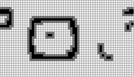
$\Lambda$${\mathcal{A}}_{1}$${\mathcal{A}}_{2}$${\mathcal{A}}_{3}$${\mathcal{A}}_{4}$

Figure 4. The space $\Lambda$ is divided into cubes; contours are formed by excited cubes (in black) and by their neighbors. There are four contours on this picture.

Summing first over admissible sets of contours $\{{\mathcal{A}}_{1},\dots,{\mathcal{A}}_{k}\}$, we can rewrite (6.1) in the following way,

$${\operatorname{Tr\,}}\,{\rm e}^{-\beta H_{\Lambda}}\,=\sum_{\{{\mathcal{A}}_{1},\dots,{\mathcal{A}}_{k}\}}\Bigl{[}\prod_{d\in D}\sum_{\omega_{W_{d}}\in\Omega_{d,W_{d}}}\,{\rm e}^{-\beta\sum_{x\in W_{d}}\Phi_{x}^{d}(\omega_{x})}\,\Bigr{]}\\ \prod_{j=1}^{k}\sum_{{\mathcal{Q}}\subset A}\sum_{m\;\geqslant\;0}\sum_{\begin{subarray}{c}{\boldsymbol{B}}_{1},\dots,{\boldsymbol{B}}_{m}\\ \bar{B}_{i}\subset{\mathcal{Q}}\end{subarray}}\sum_{\omega_{A_{j}}^{1},\dots,\omega_{A_{j}}^{m}}\int_{0<\tau_{1}<...<\tau_{m}<\beta}{\rm d}\tau_{1}\dots\rm d\tau_{m}\\ \,{\rm e}^{-\tau_{1}\sum_{x\in A_{j}}\Phi_{x}(\omega_{U(x)}^{1})}\,\langle\omega_{A_{j}}^{1}|\,T_{{\boldsymbol{B}}_{1}}\,|\omega_{A_{j}}^{2}\rangle\dots\langle\omega_{A_{j}}^{m}|\,T_{{\boldsymbol{B}}_{m}}\,|\omega_{A_{j}}^{1}\rangle\,{\rm e}^{-(\beta-\tau_{m})\sum_{x\in A_{j}}\Phi_{x}(\omega_{U(x)}^{1})}\,.$$ (6.4)

We used here the fact that the contribution of different contours factorizes. There are several restrictions to the sums over transitions $\{{\boldsymbol{B}}_{i}\}$ and configurations $\{\omega_{A_{j}}^{i}\}$: each cube of ${\mathcal{Q}}$ is intersected by at least one $\bar{B}_{i}$; $\{\omega_{A_{j}}^{i}\}$ are compatible with the labeling $\alpha_{j}$; excited cubes of $A_{j}\setminus{\mathcal{Q}}$ do not touch the boundary of ${\mathcal{A}}_{j}$; and non excited cubes in $A_{j}$ have at least one neighbor that is excited. In the last line appears configuration $\omega^{j}_{U(x)}$ with $U(x)\cap W_{d}\neq\emptyset$, hence depending on $\omega_{W_{d}}$. However, in such a case $x$ belongs to a cube that is not excited, so that $\omega^{j}_{U(x)}\in\Omega_{d,U(x)}$. From (D3) we can substitute $\Phi_{x}(\omega^{j}_{U(x)})$ with $\Phi_{x}^{d}(\omega_{x}^{j})$, which does not depend any more on the configuration outside the support of the contour. Then we obtain

$${\operatorname{Tr\,}}\,{\rm e}^{-\beta H_{\Lambda}}\,=\sum_{\{{\mathcal{A}}_{1},\dots,{\mathcal{A}}_{k}\}}\prod_{d\in D}\,{\rm e}^{-\beta h_{d}^{\beta,{\boldsymbol{\mu}}}|W_{d}|}\,\prod_{j=1}^{k}z({\mathcal{A}}_{j})$$ (6.5)

where the sum is over admissible sets of contours, and $z({\mathcal{A}})$ is the weight of the contour ${\mathcal{A}}$. The explicit expression for $z({\mathcal{A}})$ looks rather tedious, but the main point is to establish the properties of Section 3.2. The expression of $z({\mathcal{A}})$ is

$$z({\mathcal{A}})=\sum_{m\;\geqslant\;0}\sum_{{\mathcal{Q}}\subset A}\sum_{\begin{subarray}{c}{\boldsymbol{B}}_{1},\dots,{\boldsymbol{B}}_{m}\\ \bar{B}_{i}\subset{\mathcal{Q}}\end{subarray}}\sum_{\omega^{1}_{A},\dots,\omega^{m}_{A}}\int_{0<\tau_{1}<...<\tau_{m}<\beta}{\rm d}\tau_{1}\dots\rm d\tau_{m}\\ \,{\rm e}^{-\tau_{1}\sum_{x\in A}\Phi_{x}(\omega^{1}_{U(x)})}\,\langle\omega^{1}_{A}|\,T_{{\boldsymbol{B}}_{1}}\,|\omega^{2}_{A}\rangle\dots\langle\omega_{A}^{m}|\,T_{{\boldsymbol{B}}_{m}}\,|\omega_{A}^{1}\rangle\,{\rm e}^{-(\beta-\tau_{m})\sum_{x\in A}\Phi_{x}(\omega^{1}_{U(x)})}\,,$$ (6.6)

with some restrictions on the sums over $\{{\boldsymbol{B}}_{i}\}$ and $\{\omega_{A}^{i}\}$, see above.

Remark:

we constructed contours out of cubes, while the supports of contours in Section 3.2 are any connected sets. There is no contradiction, if we define the weight $z({\mathcal{A}})$ to be 0 if the support of ${\mathcal{A}}$ is not a union of cubes.

6.2. Bounds for the weights of the contours

We turn to the proof of the exponential decay of the weight of contours, as required in Section 3.2. We give the following “space-time” interpretation to the collection of sums and integrals in (6.6): we view $(\bar{B}_{j},\tau_{j})$ as a subset of $A\times[0,\beta]_{\text{\rm\,per}}$, with periodic boundary conditions along the “vertical” interval $[0,\beta]$. Furthermore, to each “time” $\tau\in[0,\beta]_{\text{\rm\,per}}$ corresponds the configuration $\omega^{j}$ for which $(\tau_{j-1},\tau_{j}]\ni\tau$. We define

$${\boldsymbol{B}}=\bigcup_{j=1}^{m}\bar{B}_{j}\times\{\tau_{j}\}\bigcup{\mathcal{Q}}\times\{0\};$$

$${\boldsymbol{E}}=\bigcup_{j=1}^{m+1}E(\omega^{j}_{\mathcal{Q}})\times[\tau_{j-1},\tau_{j}],\quad|{\boldsymbol{E}}|=\sum_{j=1}^{m+1}|E(\omega^{j}_{\mathcal{Q}})|(\tau_{j}-\tau_{j-1}),$$

(with $\tau_{0}\equiv 0$, $\tau_{m+1}\equiv\beta$, and $\omega^{m+1}\equiv\omega^{1}$). Here, we set $\bar{B}=\cup_{x\in B}U(x)$, and $E(\omega_{\mathcal{Q}})=\{x\in{\mathcal{Q}}:\omega_{U(x)}\notin\Omega_{G,U(x)}\}$.

¿From assumptions (D1) and (D2) we can bound

$$|z({\mathcal{A}})|\;\leqslant\;\,{\rm e}^{-\beta e_{0}^{\boldsymbol{\mu}}|A|}\,\sum_{m\;\geqslant\;0}\sum_{{\mathcal{Q}}\subset A}\sum_{\begin{subarray}{c}{\boldsymbol{B}}_{1},\dots,{\boldsymbol{B}}_{m}\\ \bar{B}_{i}\subset{\mathcal{Q}}\end{subarray}}\sum_{\omega^{1}_{A},\dots,\omega^{m}_{A}}\int_{0<\tau_{1}<...<\tau_{m}<\beta}{\rm d}\tau_{1}\dots\rm d\tau_{m}\\ \,{\rm e}^{-\beta\Delta|{\mathcal{E}}|/\ell^{\nu}}\,\,{\rm e}^{-\Delta_{0}|{\boldsymbol{E}}|}\,\prod_{j=1}^{m}\|T_{{\boldsymbol{B}}_{j}}\|,$$ (6.7)

where the sums over $\{{\boldsymbol{B}}_{j}\}$ and $\{\omega_{A}^{j}\}$ satisfy the restrictions explained above.

We view each $\bar{B}_{j}$ as a connected subset of ${\mathbb{R}}^{\nu+1}$ (one can e.g. add links between nearest neighbors). Then ${\boldsymbol{B}}\cup{\boldsymbol{E}}$ is a subset of ${\mathbb{R}}^{\nu+1}$ made out of vertical segments and horizontal sets. We consider connected components of ${\boldsymbol{B}}\cup{\boldsymbol{E}}$. For a connected component with $m$ horizontal sets and $m^{\prime}\;\geqslant\;m-1$ vertical segments, we deleted $m^{\prime}-m+1$ of the latters, in such a way that the component remains connected. One of these components contains ${\mathcal{Q}}\times\{0\}$, possibly with extra vertical segments and horizontal sets. Other components have $m$ horizontal sets and $m-1$ vertical segments. Because of the structure ${\bf(D4)}$, or ${\bf(B3)}$, components not linked with ${\mathcal{Q}}\times\{0\}$, either consists in a single transition of type ${\boldsymbol{K}}$, or include at least two transitions of type ${\boldsymbol{K}}$ or ${\boldsymbol{K}}^{\prime\prime}$.

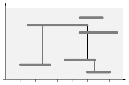
$A$$\beta$0$\bar{B}_{j}$

Figure 5. A “gather” with 6 transitions and 5 vertical segments.

A connected object with $m$ horizontal sets, and $(m-1)$ vertical segments that end on the horizontal sets, is called a gather and is denoted by the letter ${\mathcal{G}}$. It is illustrated in Fig. 5. We introduce the following sets of gathers:

• ${\mathfrak{G}}_{m}$: gathers with $m$ horizontal sets, one containing the origin $\{x=0\}\times\{\tau=0\}$; ${\mathfrak{G}}={\mathfrak{G}}_{\infty}$.

• ${\mathfrak{G}}^{\prime}$: gathers of ${\mathfrak{G}}_{1}$ that consist in a unique transition of type ${\boldsymbol{K}}$.

• ${\mathfrak{G}}_{m}^{\prime\prime}$: gathers of ${\mathfrak{G}}_{m}$, with at least two transitions of type ${\boldsymbol{K}}$ or ${\boldsymbol{K}}^{\prime\prime}$; ${\mathfrak{G}}={\mathfrak{G}}_{\infty}^{\prime\prime}$.

The connected component of ${\boldsymbol{B}}\cup{\boldsymbol{E}}$ that contains ${\mathcal{Q}}\times\{0\}$ can be viewed as a set of gathers, each gather being connected to ${\mathcal{Q}}\times\{0\}$ by a vertical segment.

Since a choice of $\{{\boldsymbol{B}}_{i}\}$ and $\{\omega_{\mathcal{Q}}^{i}\}$ leads to a set of gathers, we obtain a bound by first integrating over sets of gathers, then summing over compatible space-time configurations ${\boldsymbol{\omega}}_{A}$, and choosing which gathers are linked to ${\mathcal{Q}}\times\{0\}$. Therefore

$$|z({\mathcal{A}})|\;\leqslant\;\,{\rm e}^{-\beta e_{0}^{\boldsymbol{\mu}}|A|}\,\sum_{k\;\geqslant\;0}\frac{1}{k!}\int{\rm d}{\mathcal{G}}_{1}\dots\rm d{\mathcal{G}}_{k}\sum_{{\boldsymbol{\omega}}_{A}}\sum_{\text{links}}\,{\rm e}^{-\beta\Delta|{\mathcal{E}}|/\ell^{\nu}}\,\,{\rm e}^{-\Delta_{0}|{\boldsymbol{E}}|}\,\prod_{j=1}^{k}\Bigl{(}\prod_{{\boldsymbol{B}}\in{\mathcal{G}}_{j}}\|T_{\boldsymbol{B}}\|\Bigr{)}.$$ (6.8)

The shortcut $\int{\rm d}{\mathcal{G}}$ means a sum over the number $m$ of transitions, a sum over transitions ${\boldsymbol{B}}_{1},\dots,{\boldsymbol{B}}_{m}$, an integral over ordered times $\tau_{1},\dots,\tau_{m}$, and a sum over $(m-1)$ vertical segments that link $\bigl{\{}\bar{B}_{i}\times\{\tau_{i}\}\bigr{\}}$ together.

We define

$$\tilde{z}({\mathcal{G}})=\,{\rm e}^{-\Delta_{0}|{\mathcal{G}}|}\,\prod_{{\boldsymbol{B}}\in{\mathcal{G}}}\|T_{\boldsymbol{B}}\|\,{\rm e}^{2\nu\ell^{\nu}(\log M+\tau)|\bar{B}|}\,,$$ (6.9)

where $|{\mathcal{G}}|$ is the total length of the vertical segments of ${\mathcal{G}}$. If $\beta\Delta/\ell^{\nu}\;\geqslant\;2\nu(\log M+\tau)$, we can write

$$z({\mathcal{A}})|\,{\rm e}^{\tau|A|}\,\;\leqslant\;\,{\rm e}^{-\beta e_{0}^{\boldsymbol{\mu}}|A|}\,\sum_{k\;\geqslant\;0}\frac{(2|{\mathcal{Q}}|)^{k}}{k!}\Bigl{(}\int_{0}^{\beta}{\rm d}\tau\,{\rm e}^{-\Delta_{0}\tau}\,\int_{\mathfrak{G}}{\rm d}{\mathcal{G}}\tilde{z}({\mathcal{G}})\Bigr{)}^{k}\\ \sum_{k\;\geqslant\;0}\frac{|{\mathcal{Q}}|^{k}}{k!}\Bigl{(}\int_{0}^{\beta}{\rm d}\tau\int_{{\mathfrak{G}}^{\prime}\cup{\mathfrak{G}}^{\prime\prime}}{\rm d}{\mathcal{G}}\tilde{z}({\mathcal{G}})\Bigr{)}^{k},$$ (6.10)

where the first sum corresponds to the number of gathers linked to ${\mathcal{Q}}\times\{0\}$, and the second sum is the number of independent gathers. The shortcut $\int_{\mathfrak{G}}{\rm d}{\mathcal{G}}$ is identical to $\int{\rm d}{\mathcal{G}}$, except for the absence of an integral over $\tau_{1}$, which is set to 0; integrals over ${\mathfrak{G}}^{\prime}$ and ${\mathfrak{G}}^{\prime\prime}$ are similar.

One easily obtains an upper bound for the gathers with a unique transition:

$$\int_{{\mathfrak{G}}^{\prime}}{\rm d}{\mathcal{G}}\tilde{z}({\mathcal{G}})=\sum_{B,\bar{B}\ni 0}\|K_{B}\|\,{\rm e}^{2\nu\ell^{\nu}(\log M+\tau)|\bar{B}|}\,\;\leqslant\;(2R+1)^{\nu}\|{\boldsymbol{K}}\|_{c}$$ (6.11)

with $c=2\nu\ell^{\nu}(2R+1)^{\nu}(\log M+\tau)$; this is smaller than $\Delta_{0}$ if $c$ is large enough in the assumptions of Theorem 4.4.

For general gathers, we proceed by induction. First,

$$\int_{{\mathfrak{G}}_{1}}{\rm d}{\mathcal{G}}\tilde{z}({\mathcal{G}})\;\leqslant\;(2R+1)^{\nu}\bigl{(}\|{\boldsymbol{K}}\|_{c}+\|{\boldsymbol{K}}^{\prime}\|_{c}+\|{\boldsymbol{K}}^{\prime\prime}\|_{c}\bigr{)}.$$ (6.12)

Next, we use the recursion inequality:

$$\int_{{\mathfrak{G}}_{m}}{\rm d}{\mathcal{G}}\tilde{z}({\mathcal{G}})\;\leqslant\;\sum_{{\boldsymbol{B}},\bar{B}\ni 0}\|T_{\boldsymbol{B}}\|\,{\rm e}^{2\nu\ell^{\nu}(\log M+\tau)|\bar{B}|}\,\\ \sum_{k\;\geqslant\;0}\frac{1}{k!}\Bigl{(}2\sum_{y\in\bar{B}}\int_{0}^{\beta}{\rm d}\tau\,{\rm e}^{-\Delta_{0}\tau}\,\int_{{\mathfrak{G}}_{m-1,0}}{\rm d}{\mathcal{G}}\tilde{z}({\mathcal{G}})\Bigr{)}^{k}.$$ (6.13)

Integrating over $\tau$, and since $\|{\boldsymbol{K}}^{\boldsymbol{\cdot}}\|_{c}/\Delta_{0}\;\leqslant\;1$ for a large enough $c$, we get

$$\int_{{\mathfrak{G}}_{m}}{\rm d}{\mathcal{G}}\tilde{z}({\mathcal{G}}) \;\leqslant\;\sum_{{\boldsymbol{B}},\bar{B}\ni 0}\|T_{\boldsymbol{B}}\|\,{\rm e}^{2\nu\ell^{\nu}(\log M+\tau)|\bar{B}|}\,\,{\rm e}^{2|\bar{B}|}\,$$

$$\;\leqslant\;(2R+1)^{\nu}\bigl{(}\|{\boldsymbol{K}}\|_{c}+\|{\boldsymbol{K}}^{\prime}\|_{c}+\|{\boldsymbol{K}}^{\prime\prime}\|_{c}\bigr{)}.$$ (6.14)

This holds independently of $m$. This allows to estimate the integral over gathers that contain at least two transitions of type ${\boldsymbol{K}}$ or ${\boldsymbol{K}}^{\prime\prime}$. Let ${\mathfrak{G}}_{m}^{\prime}\subset{\mathfrak{G}}_{m}$ be gathers with at least one transition of type ${\boldsymbol{K}}$ or ${\boldsymbol{K}}^{\prime}$. One easily obtains

$$\int_{{\mathfrak{G}}_{m}}{\rm d}{\mathcal{G}}\tilde{z}({\mathcal{G}})\;\leqslant\;(2R+1)^{\nu}\bigl{(}\|{\boldsymbol{K}}\|_{c}+\|{\boldsymbol{K}}^{\prime\prime}\|_{c}\bigr{)}.$$ (6.15)

Then the integral over gathers with two transitions of type ${\boldsymbol{K}}$ or ${\boldsymbol{K}}^{\prime\prime}$ can be done by integrating first on the time for such a transition, then over vertical segments and gathers at their ends, at least one of which must belong to ${\mathfrak{G}}_{m-1}^{\prime}$. We obtain

$$\int_{0}^{\beta}{\rm d}\tau \sum_{B,\bar{B}\subset{\mathcal{Q}}}(\|K_{B}\|+\|K_{B}^{\prime\prime}\|)\,{\rm e}^{2\nu\ell^{\nu}(\log M+\tau)|\bar{B}|}\,\int_{0}^{\beta}{\rm d}\tau^{\prime}\,{\rm e}^{-\Delta_{0}\tau^{\prime}}\,\int_{{\mathfrak{G}}_{m-1}^{\prime}}{\rm d}{\mathcal{G}}\tilde{z}({\mathcal{G}})$$

$$\hskip 128.0374pt\sum_{k\;\geqslant\;0}\frac{1}{k!}\Bigl{(}2\sum_{y\in\bar{B}}\int_{0}^{\beta}{\rm d}\tau\,{\rm e}^{-\Delta_{0}\tau}\,\int_{{\mathfrak{G}}_{m-1,0}}{\rm d}{\mathcal{G}}\tilde{z}({\mathcal{G}})\Bigr{)}^{k}$$

$$\;\leqslant\;\beta|{\mathcal{Q}}|\frac{(\|{\boldsymbol{K}}\|_{c}+\|{\boldsymbol{K}}^{\prime\prime}\|_{c})^{2}}{\Delta_{0}}.$$ (6.16)

Plugging these estimates in (6.10), one easily gets

$$z({\mathcal{A}})\,{\rm e}^{\tau|A|}\,\;\leqslant\;\,{\rm e}^{-\beta e_{0}^{\boldsymbol{\mu}}|A|}\,\,{\rm e}^{3|A|}\,.$$ (6.17)

Exponential decay of the weights of the contours is now clear.

The bound on the derivative can be proven in the same way. Looking at (6.6), we see that the integrand gets a factor bounded by $\beta|A|\sup_{x,{\boldsymbol{\mu}},\omega,j}|\frac{\partial}{\partial{\boldsymbol{\mu}}_{j}}\Phi_{x}(\omega_{U(x)})|$.

6.3. Other properties of the weights

The weight of the contours can be viewed as a series in powers of $\{K_{B}\}$, $\{K_{B}^{\prime}\}$, $\{K_{B}^{\prime\prime}\}$. Since it is absolutely convergent uniformly in ${\boldsymbol{K}}$, ${\boldsymbol{K}}^{\prime}$, ${\boldsymbol{K}}^{\prime\prime}$ (provided they be small enough), we have by the dominated convergence theorem

$$\lim_{{\boldsymbol{K}},{\boldsymbol{K}}^{\prime},{\boldsymbol{K}}^{\prime\prime}\to 0}z({\mathcal{A}})=0.$$ (6.18)

Analyticity of $z({\mathcal{A}})$ as function of ${\boldsymbol{\mu}}$ and $\beta$ is clear, as well as a function of $\eta$ if we add a new perturbation $\eta{\boldsymbol{L}}$, in a neighborhood of 0 that depends on $\beta\|{\boldsymbol{L}}\|$. Periodicity is also obvious.

Acknowledgments: It is a pleasure to thank Roberto Fernández, Roman Kotecký, and Charles-Édouard Pfister for several discussions, and the referee for useful comments.

References

- [1]
- [Ara] H. Araki, On the equivalence of the KMS condition and the variational principle for quantum lattice systems, Commun. Math. Phys. 38, 1–10 (1974)
- [BI] C. Borgs and J. Imbrie, A unified approach to phase diagrams in field theory and statistical mechanics, Commun. Math. Phys. 123, 305–328 (1989)
- [BJK] C. Borgs, J. Jȩdrzejewski and R. Kotecký, The staggered charge-order phase of the extended Hubbard model in the atomic limit, J. Phys. A 29, 733–747 (1996)
- [BK] C. Borgs and R. Kotecký, A rigorous theory of finite-size scaling at first-order phase transitions, J. Stat. Phys. 61, 79–119 (1990)
- [BK2] C. Borgs and R. Kotecký, Surfaced induced finite size effects for first order phase transitions, J. Stat. Phys. 79, 43–115 (1994)
- [BK3] C. Borgs and R. Kotecký, Low temperature phase diagrams of fermionic lattice systems, Commun. Math. Phys. 208, 575–604 (2000)
- [BKU] C. Borgs, R. Kotecký and D. Ueltschi, Low temperature phase diagrams for quantum perturbations of classical spin systems, Commun. Math. Phys. 181, 409–446 (1996)
- [BW] C. Borgs and R. Waxler, First order phase transitions in unbounded spin systems. II. Completeness of the phase diagram, Commun. Math. Phys. 126, 483–506 (1990)
- [BR] O. Bratteli and D. W. Robinson, Operator Algebras and Quantum Statistical Mechanics I and II, Springer-Verlag (1981)
- [BKL] J. Bricmont, K. Kuroda and J. L. Lebowitz, First order phase transitions in lattice and continuous systems: Extension of Pirogov-Sinai theory, Commun. Math. Phys. 101, 501–538 (1985)
- [BS] J. Bricmont and J. Slawny, Phase transitions in systems with a finite number of dominant ground states, J. Stat. Phys. 54, 89–161 (1989)
- [DFF] N. Datta, R. Fernández and J. Fröhlich, Low-temperature phase diagrams of quantum lattice systems. I. Stability for quantum perturbations of classical systems with finitely-many ground states, J. Stat. Phys. 84, 455–534 (1996)
- [DFF2] N. Datta, R. Fernández and J. Fröhlich, Effective Hamiltonians and phase diagrams for tight-binding models, J. Stat. Phys. 96, 545–611 (1999)
- [DFFR] N. Datta, R. Fernández, J. Fröhlich and L. Rey-Bellet, Low-temperature phase diagrams of quantum lattice systems. II. Convergent perturbation expansions and stability in systems with infinite degeneracy, Helv. Phys. Acta 69, 752–820 (1996)
- [DLS] F. J. Dyson, E. H. Lieb and B. Simon, Phase transitions in quantum spin systems with isotropic and nonisotropic interactions, J. Stat. Phys. 18, 335–383 (1978)
- [EFS] A. van Enter, R. Fernández and A. D. Sokal, Regularity properties and pathologies of position-space renormalization-group transformations: scope and limitations of gibbsian theory, J. Stat. Phys. 72, 879–1167 (1993)
- [FL] J. Fröhlich and E. H. Lieb, Phase transitions in anisotropic lattice spin systems, Commun. Math. Phys. 60, 233-267 (1978)
- [FR] J. Fröhlich and L. Rey-Bellet, Low-temperature phase diagrams of quantum lattice systems. III. Examples, Helv. Phys. Acta 69, 821-849 (1996)
- [FSS] J. Fröhlich, B. Simon and T. Spencer, Infrared bounds, phase transitions and continuous symmetry breaking, Commun. Math. Phys. 50, 79–95 (1976)
- [GKU] Ch. Gruber, R. Kotecký and D. Ueltschi, Planar and lamellar antiferromagnetisms in Hubbard models, J. Phys. A 33, 7857–7871 (2000)
- [Isr] R. B. Israel, Convexity in the Theory of Lattices Gases, Princeton University Press (1979)
- [Jȩd] J. Jȩdrzejewski, Phase diagrams of extended Hubbard models in the atomic limit, Physica A 205, 702–717 (1994)
- [KP] R. Kotecký and D. Preiss, An inductive approach to Pirogov-Sinai theory, Suppl. ai rendiconti del circilo matem. di Palermo, ser. II 3, 161–164 (1984)
- [KU] R. Kotecký and D. Ueltschi, Effective interactions due to quantum fluctuations, Commun. Math. Phys. 206, 289–335 (1999)
- [Lieb] E. H. Lieb, The Hubbard model: some rigorous results and open problems, XIth Internat. Congress of Math. Physics (Paris, 1994), 392–412, Internat. Press (1995)
- [Pei] R. Peierls, On the Ising model of ferromagnetism, Proc. Cambridge Philos. Soc. 32, 477-481 (1936)
- [Pir] S. A. Pirogov, Phase diagrams of quantum lattice systems, Soviet Math. Dokl. 19, 1096–1099 (1978)
- [PS] S. A. Pirogov and Ya. G. Sinai, Phase diagrams of classical lattice systems, Theoretical and Mathematical Physics 25, 1185–1192 (1975); 26, 39–49 (1976)
- [Rue] D. Ruelle, Statistical Mechanics: Rigorous Results, W. A. Benjamin (1969)
- [Sim] B. Simon, The Statistical Mechanics of Lattice Gases, Princeton Univ. Press (1993)
- [Sin] Ya. G. Sinai, Theory of Phase Transitions: Rigorous Results, Pergamon Press (1982)
- [Uel] D. Ueltschi, Analyticity in Hubbard models, J. Stat. Phys. 95, 693–717 (1999)
- [Zah] M. Zahradník, An alternate version of Pirogov-Sinai theory, Commun. Math. Phys. 93, 559–581 (1984)