IHES-P/00/42

Abstract

A simple, but not widely known, mathematical fact concerning the coverings of the full Lorentz group sheds light on parity and time reversal transformations of fermions. Whereas there is, up to an isomorphism, only one Spin group which double covers the orientation preserving Lorentz group, there are two essentially different groups, called Pin groups, which cover the full Lorentz group. Pin(1,3) is to O(1,3) what Spin(1,3) is to SO(1,3). The existence of two Pin groups offers a classification of fermions based on their properties under space or time reversal finer than the classification based on their properties under orientation preserving Lorentz transformations — provided one can design experiments that distinguish the two types of fermions. Many promising experimental setups give, for one reason or another, identical results for both types of fermions. These negative results are reported here because they are instructive. Two notable positive results show that the existence of two Pin groups is relevant to physics:

• In a neutrinoless double beta decay, the neutrino emitted and reabsorbed in the course of the interaction can only be described in terms of Pin(3,1).

• If a space is topologically nontrivial, the vacuum expectation values of Fermi currents defined on this space can be totally different when described in terms of Pin(1,3) and Pin(3,1).

Possibly more important than the two above predictions, the Pin groups provide a simple framework for the study of fermions; it makes possible clear definitions of intrinsic parities and time reversal; it clarifies colloquial, but literally meaningless, statements. Given the difference between the Pin group and the Spin group it is useful to distinguish their representations, as groups of transformations on “pinors” and “spinors”, respectively.  
 
The Pin(1,3) and Pin(3,1) fermions are twin-like particles whose behaviors differ only under space or time reversal.  
 
A section on Pin groups in arbitrary spacetime dimensions is included.

The Pin Groups in Physics:
$C$, $P$, and $T$

Table of contents

• Dictionary of Notation

• Introduction

• Background

  • As seen by physicists

    • Superselection rules

    • Parity violation

    • Standard Model

  • As seen by Wigner

  • As seen by mathematicians

• The Pin groups in 3 space, 1 time dimensions

  • The Pin groups

    • Pin(1,3)

    • Pin(3,1)

  • A Spin group is a subgroup of a Pin group

  • Pin group and Spin group representations on finite-dimensional spaces; classical fields.

    • Pinors

    • Spinors

    • Helicity

    • Massless spinors, massive pinors

    • Copinors, Dirac and Majorana adjoints

    • Charge conjugate pinors in Pin(1,3)

    • Majorana pinors

    • Unitary and antiunitary transformations

    • Invariance of the Dirac equation under antiunitary transformations

    • $C\!PT$ invariance

    • Charge conjugate pinors in Pin(3,1)

  • Pin group and Spin group representations on infinite-dimensional spaces; quantum fields.

    • Particles, antiparticles

    • Fock space operators, unitary and antiunitary

    • Intrinsic parity

    • Majorana field operator

    • Majorana classical field vs. Majorana quantum field

    • $C\!PT$ transformations

  • Bundles; Fermi fields on manifolds

    • Pinor coordinates

    • Dirac adjoint in Pin(1,3)

    • Dirac adjoint in Pin(3,1)

    • Pin structures

    • Fermi fields on topologically nontrivial manifolds

  • Bundle reduction

• Search For Observable Differences

  • Computing observables with Pin(1,3) and Pin(3,1)

  • Parity and the Particle Data Group publications

    • Parity conservation

  • Determining parity experimentally

    • Selection rules: Pion decay

    • Selection rules: Three-fermion decay

    • Selection rules: Positronium

    • Decay rates; cross sections

  • Interference, reversing magnetic fields, reflection

  • Time reversal and Kramer’s degeneracy

  • Charge conjugation

    • Positronium

    • Neutrinoless double beta decay

• The Pin groups in $s$ space, $t$ time dimensions

  • The difference between $s+t$ even and $s+t$ odd

    • The twisted map

  • Chirality

  • Construction of gamma matrices; periodicity modulo 8

    • Onsager construction of gamma matrices

    • Majorana pinors, Weyl-Majorana spinors

  • Conjugate and complex gamma matrices

  • The short exact sequence $1{\rm I}\rightarrow$ Spin$(t,s)\rightarrow$ Pin$(t,s)\rightarrow{\mathbb{Z}}_{2}\rightarrow 0$

  • Grassman (superclassical) pinor fields

  • String theory and pin structures

• Conclusion

  • Some facts

  • A tutorial

    • Parity

    • Time reversal

    • Charge conjugation

    • Wigner’s classification and classification by Pin groups

    • Fock space and one-particle states

  • Avenues to explore

Appendices

• Induced transformations

• The isomorphism of $M_{4}({\mathbb{R}})$ and ${\mathbb{H}}\otimes{\mathbb{H}}$

• Other double covers of the Lorentz group

• Collected calculations

• Collected references

0 Dictionary of Notation

The article proper begins with section 1.  
 
We have occasionally changed some of our earlier notations to conform to the majority of users. As much as possible, we have tried to use the usual notation – but introducing different symbols for different objects when it is essential to distinguish them. For example, we distinguish the Spin group and the two Pin groups (sometimes still known as Spin groups) but we speak globally of spin 1/2 particles (lower case “s”) for all particles, whether they are represented by spinors or pinors of either type. This agrees with intuitive notion of spin as “the behavior of a field or a state under rotations” [88].  
 
Our primary references are Peskin and Schroeder [87], Weinberg [115] and Choquet-Bruhat et al. [28, 30].  
 
  
 
Groups

• Lorentz group

  • • O(1,3) leaves $\eta_{\alpha\beta}x^{\alpha}x^{\beta}$ invariant, $\eta_{\alpha\beta}={\rm diag}(1,-1,-1,-1)$
      with $\alpha,\beta\in\{0,1,2,3\}$, $x^{0}=t$

    • O(3,1) leaves $\hat{\eta}_{\alpha\beta}x^{\alpha}x^{\beta}$ invariant, $\hat{\eta}_{\alpha\beta}={\rm diag}(1,1,1,-1)$
      with $\alpha,\beta\in\{1,2,3,4\}$, $x^{4}=t$

  • Examples:
    Reverse $({L^{\alpha}}_{\beta})\in\mathrm{O}(1,3)$ $(\hat{L}^{\alpha}{}_{\beta})\in\mathrm{O}(3,1)$ 1 space axis $P(1)={\rm diag}(1,1,1,-1)$ $\hat{P}(1)={\rm diag}(-1,1,1,1)$ 3 space axes $P(3)={\rm diag}(1,-1,-1,-1)$ $\hat{P}(3)={\rm diag}(-1,-1,-1,1)$ time axis $T={\rm diag}(-1,1,1,1)$ $\hat{T}={\rm diag}(1,1,1,-1)$

  $${L^{\alpha}}_{\beta}{(L^{-1})^{\beta}}_{\gamma}=\delta^{\alpha}_{\beta}\;,\qquad LL^{T}=1{\rm I}\mbox{ hence }{(L^{-1})^{\beta}}_{\gamma}={L_{\gamma}}^{\beta}\;.$$

• Real Clifford algebra

  • The Clifford algebra is a graded algebra ${\mathcal{C}}={\mathcal{C}}_{+}\oplus{\mathcal{C}}_{-}\;.$
    ${\mathcal{C}}_{+}$ is generated by even products of $\gamma_{\alpha}$’s, $\Lambda^{\rm even}\in{\mathcal{C}}_{+}$
    ${\mathcal{C}}_{-}$ is generated by odd products of $\gamma_{\alpha}$’s, $\Lambda^{\rm odd}\in{\mathcal{C}}_{-}$.

  • We choose  
    $\{\gamma_{\alpha},\gamma_{\beta}\}=2\eta_{\alpha\beta}\qquad\{\hat{\gamma}_{\alpha},\hat{\gamma}_{\beta}\}=2\hat{\eta}_{\alpha\beta}$
    

  • We could also fix the signature of the metric and have $\{\hat{\gamma}_{\alpha}\hat{\gamma}_{\beta}\}=-2\eta_{\alpha\beta}$, but we prefer to associate $\hat{\gamma}_{\alpha}$ with $\hat{\eta}_{\alpha\beta}$ rather than with  $-\eta_{\alpha\beta}$.
    

• Pin groups

  • $\Lambda_{L}\in{\rm Pin}{}(1,3)$	$\Leftrightarrow$	$\Lambda_{L}\gamma_{\alpha}\Lambda_{L}^{-1}=\gamma_{\beta}{L^{\beta}}_{\alpha}$	or	$\Lambda_{L}\gamma^{\alpha}\Lambda_{L}^{-1}={(L^{-1})^{\alpha}}_{\beta}\gamma^{\beta}$
    $\hat{\Lambda}_{L}\in{\rm Pin}{}(3,1)$	$\Leftrightarrow$	$\hat{\Lambda}_{L}\hat{\gamma}_{\alpha}\hat{\Lambda}_{L}^{-1}=\hat{\gamma}_{\beta}{\left.\hat{L}^{\beta}\right.}_{\alpha}$	or	$\hat{\Lambda}_{L}\hat{\gamma}^{\alpha}\hat{\Lambda}_{L}^{-1}={(\hat{L}^{-1})^{\alpha}}_{\beta}\hat{\gamma}^{\beta}$

    
    

  • Examples:

    $$\begin{array}[]{lclclcl}\Lambda_{P(1)}&=&\pm\gamma_{0}\gamma_{1}\gamma_{2}&&\hat{\Lambda}_{P(1)}&=&\pm\hat{\gamma}_{2}\hat{\gamma}_{3}\hat{\gamma}_{4}\\ \Lambda_{P(3)}&=&\pm\gamma_{0}&&\hat{\Lambda}_{P(3)}&=&\pm\hat{\gamma}_{4}\\ \Lambda_{T}&=&\pm\gamma_{1}\gamma_{2}\gamma_{3}&&\hat{\Lambda}_{T}&=&\pm\hat{\gamma}_{1}\hat{\gamma}_{2}\hat{\gamma}_{3}\\ \Lambda_{P(1)}^{2}&=&-1{\rm I}&&\hat{\Lambda}_{P(1)}^{2}&=&+1{\rm I}\\ \Lambda_{P(3)}^{2}&=&+1{\rm I}&&\hat{\Lambda}_{P(3)}^{2}&=&-1{\rm I}\\ \Lambda_{T}^{2}&=&+1{\rm I}&&\hat{\Lambda}_{T}^{2}&=&-1{\rm I}\end{array}$$

• Spin group

  • ${\rm Spin}(1,3)\subset{\rm Pin}(1,3)\qquad{\rm Spin}(3,1)\subset{\rm Pin}(3,1)$
    

  • A Spin group consists of elements $\Lambda_{L}$ for $L$ such that $\det({L^{\beta}}_{\alpha})=1$. It consists of even elements (even products of $\gamma_{\alpha}$) of a Pin group.
    

  • $${\rm Pin}(m,n)={\rm Spin}(m,n)\ltimes{\mathbb{Z}}_{2}\qquad\mbox{for $m+n>1$}$$

    ($\ltimes$ is a semidirect product, defined in sec. 5.5).

Group representations, unitary and antiunitary

• On finite-dimensional vector spaces, real or complex:

  • $\Gamma_{\alpha}$ is a real or complex matrix representation of $\gamma_{\alpha}$.

  • $\hat{\Gamma}_{\alpha}$ is a real or complex matrix representation of $\hat{\gamma}_{\alpha}$,

    $$\hat{\Gamma}_{\alpha}=i\Gamma_{\alpha}\;.$$

  • Chiral representation

    $$\begin{array}[]{rclrcl}\Gamma_{0}&=&\left(\begin{array}[]{cccc}\;0&\;0&\;1&\;0\\ 0&0&0&1\\ 1&0&0&0\\ 0&1&0&0\end{array}\right)\;,&\Gamma_{1}&=&\left(\begin{array}[]{cccc}0&0&\;0&\;1\\ 0&0&1&0\\ 0&-1&0&0\\ -1&0&0&0\end{array}\right)\\[28.45274pt] \Gamma_{2}&=&\left(\begin{array}[]{cccc}0&\;0&\;0&-i\\ 0&0&i&0\\ 0&i&0&0\\ -i&0&0&0\end{array}\right)\;,&\Gamma_{3}&=&\left(\begin{array}[]{cccc}0&\;0&\;1&0\\ 0&0&0&-1\\ -1&0&0&0\\ 0&1&0&0\end{array}\right)\end{array}$$

    $$\Gamma_{5}=i\Gamma_{0}\Gamma_{1}\Gamma_{2}\Gamma_{3}=\left(\begin{array}[]{cccc}-1&0&\;0&\;0\\ 0&-1&0&0\\ 0&0&1&0\\ 0&0&0&1\end{array}\right)\;.$$

  • Dirac representation, exchange $\Gamma_{0}$ above for

    $$\Gamma_{0}=\left(\begin{array}[]{cccc}\;1&\;0&0&0\\ 0&1&0&0\\ 0&0&-1&0\\ 0&0&0&-1\end{array}\right)\;.$$

    $\Gamma_{1}$, $\Gamma_{2}$, $\Gamma_{3}$ are the same as in the chiral representation.  
    

  • A Majorana (real) representation in Pin(3,1):

    $$\begin{array}[]{rclrcl}\hat{\Gamma}_{1}&=&\left(\begin{array}[]{cccc}0&\;0&\;0&-1\\ 0&0&1&0\\ 0&1&0&0\\ -1&0&0&0\end{array}\right)\;,&\hat{\Gamma}_{2}&=&\left(\begin{array}[]{cccc}\;1&\;0&0&0\\ 0&1&0&0\\ 0&0&-1&0\\ 0&0&0&-1\end{array}\right)\\[28.45274pt] \hat{\Gamma}_{3}&=&\left(\begin{array}[]{cccc}0&0&-1&0\\ 0&0&0&-1\\ -1&0&0&0\\ 0&-1&0&0\end{array}\right)\;,&\hat{\Gamma}_{4}&=&\left(\begin{array}[]{cccc}0&0&\;0&\;1\\ 0&0&1&0\\ 0&-1&0&0\\ -1&0&0&0\end{array}\right)\end{array}$$

  • Pauli matrices

    $$\sigma_{1}=\left(\begin{array}[]{cc}\;0&\;1\\ 1&0\end{array}\right)\;,\quad\sigma_{2}=\left(\begin{array}[]{cc}\;0&-i\\ i&0\end{array}\right)\;,\quad\sigma_{3}=\left(\begin{array}[]{cc}\;1&0\\ 0&-1\end{array}\right)\;,\quad$$

  • Dirac equation for a massive, charged particle

    $$(i\Gamma^{\alpha}\nabla_{\alpha}-m)\psi(x)=0\qquad\qquad(\hat{\Gamma}^{\alpha}\nabla_{\alpha}-m)\hat{\psi}(x)=0$$

    $$\mbox{ with }\nabla_{\alpha}=\partial_{\alpha}+iqA_{\alpha}$$

  • Dirac adjoint (see 3.5 for Dirac adjoints on general manifolds)

    $$\bar{\psi}=\psi^{\dagger}\,\Gamma_{0}\;,\qquad\bar{\hat{\psi}}=\hat{\psi}^{\dagger}\hat{\Gamma}_{4}\;.$$

  • Charge conjugate

    $$(i\Gamma^{\alpha}(\partial_{\alpha}-iqA_{\alpha})-m)\psi^{\rm c}(x)=0\;,\qquad(\hat{\Gamma}^{\alpha}(\partial_{\alpha}-iqA_{\alpha})-m)\hat{\psi}^{\rm c}(x)=0$$

    and $\psi^{\rm c}={\mathcal{C}}\psi^{*}$, $\hat{\psi}^{\rm c}=\hat{\mathcal{C}}\hat{\psi}^{*}$, where

    $${\mathcal{C}}\,\Gamma_{\alpha}^{*}{\mathcal{C}}^{-1}=-\Gamma_{\alpha}\;,\qquad\hat{\mathcal{C}}\,\hat{\Gamma}_{\alpha}^{*}\hat{\mathcal{C}}^{-1}=\hat{\Gamma}_{\alpha}\;.$$

    In the Dirac representation ${\mathcal{C}}=\pm\Gamma_{2}$, $\hat{\mathcal{C}}=\pm\hat{\Gamma}_{2}$ and ${\mathcal{C}}{\mathcal{C}}^{*}=1{\rm I}$, $\hat{\mathcal{C}}\hat{\mathcal{C}}^{*}=1{\rm I}$.

  
  

• Two-component fermions, Weyl fermions

  $${\mathcal{P}}_{\pm}={\scriptstyle{1\over 2}}(1{\rm I}\pm\Gamma_{5})$$

  $${\mathcal{P}}_{+}\psi = \varphi_{R}\qquad\mbox{chirality $+1$}$$

  $${\mathcal{P}}_{-}\psi = \varphi_{L}\qquad\mbox{chirality $-1$}$$

• The antiunitary time reversal operator ${\mathcal{A}}_{T}$ on $\psi$ acts on the complex conjugate $\psi^{*}$,

  $${\mathcal{A}}_{T}{\mathcal{C}}^{-1}=\Lambda_{T}\;.$$

  
  

• On infinite-dimensional Hilbert spaces of state vectors:

  • Quantum fields (see 3.4)

    $$\Psi(x) = {1\over\sqrt{\Omega}}\sum_{p,s}\left(a({\bf p},s)\psi(p,s)+b^{\dagger}({\bf p},s)\psi^{\rm c}(p,s)\right)$$

    $$\Psi^{\rm c}(x) = {\xi\over\sqrt{\Omega}}\sum_{p,s}\left(b({\bf p},s)\psi(p,s)+a^{\dagger}({\bf p},s)\psi^{\rm c}(p,s)\right)\;.$$

    where $\sum_{p,s}$ combines $\sum_{s}$ and $\int d^{4}p\,\delta(p^{2}-m^{2})$, and $\xi$ is a phase, $|\xi|=1$.  
    

  • States

    • States are created by applying creation and annihilation operators on the vacuum state, e.g.

      $$\left\{\begin{array}[]{l}\Psi(x)|0\rangle={1\over\sqrt{\Omega}}\sum_{p,s}b^{\dagger}({\bf p},s)\psi^{\rm c}(p,s)|0\rangle\\ \langle b|\Psi(x)|0\rangle=\psi^{\rm c}(p,s)\end{array}\right.$$

      $\psi$, $\psi^{\rm c}$ are called classical fields even when they are fermionic; the space of classical fields is the domain of the classical action (the classical action is not to be confused with its minimum value).
      

    • $\Psi(x)|0\rangle$ is a linear superposition of one-antiparticle states of well-defined momentum $p$ and spin polarization $s$.

1 Introduction

A simple, but not widely known, mathematical fact concerning the coverings of the full Lorentz group sheds light on parity and time reversal transformations of fermions. Whereas there is, up to an isomorphism, only one Spin group which double covers the orientation preserving Lorentz group, there are two essentially different groups, called Pin groups, which cover the full Lorentz group. The name Pin is gaining acceptance because it is a useful name: Pin(1,3) is to O(1,3) what Spin(1,3) is to SO(1,3). The existence of two Pin groups explains several issues which we discuss in section 2. It offers a classification of fermions based on their properties under space or time reversal finer than the classification based on their properties under orientation preserving Lorentz transformations.  
 
For the convenience of the reader, we have divided this report into two parts: in the first part we present the Pin groups for three space dimensions and one time dimension; in the second part we present the Pin groups for $s$ space dimensions and $t$ time dimensions (with emphasis on the hyperbolic case $t=1$). In appendix E we have collected, by topic, references of related articles which we have consulted.

2 Background

2.1 As seen by physicists

Racah, in 1937 [90], and Yang and Tiomno, in 1950 [126], pointed out that under a space inversion four different transformations for fields of spin 1/2 are possible. Yang and Tiomno added, “The types of transformation properties to which the various known spin-1/2 fields belong are physical observables and could in principle be determined experimentally from their mutual interactions and their interactions with fields of integral spin.”. They wrote down a list of all possible spinor interactions using the four types of spinors, and attempted to exclude some interactions based on the guiding principle of parity conservation. Fermi even scheduled a special session at a conference he organized in Chicago (September 1951) devoted to these ideas and to the experimental distinction between the different kinds of spinors [121].  
 
Under the impact of superselection rules [120], the discovery of parity violation [62, 124], and the success of the Standard Model [97, 98, 114], the Yang and Tiomno paper fell by the wayside; its goal was rendered obsolete. Nevertheless the fact remains that there are four different kinds of spin-1/2 particles. Why has this fact, noted already in 1937, been largely ignored?  
 
a) The impact of superselection rules in the 1960s
In 1952, Wick, Wightman, and Wigner discussed limitations of the concept of intrinsic parity of elementary particles, in a paper affectionately known as W³ [120]. These limitations follow from superselection rules — rules which restrict the nature and scope of possible measurements. More precisely, there is a superselection rule if the following conditions are satisfied: i) there is an exact conservation law, and ii) the Hilbert space can be decomposed into orthogonal subspaces $\{{\mathcal{H}}_{1},{\mathcal{H}}_{2},\ldots\}$ such that there are no observables which contain matrix elements between any pair of those subspaces, thus making the relative phases between components of the state vector in different subspaces ${\mathcal{H}}_{i}$ and ${\mathcal{H}}_{j}(i\neq j)$ irrelevant.  
 
In particular, these restrictions cast a shadow on the possibility of identifying Dirac fields by their transformation properties under space inversion. But it has been shown [36] that the four choices of Pin structure are observable—admittedly in an exotic setting, but even such an example is sufficient to rule out a Pin superselection rule operating in general. Moreover, as pointed out by Weinberg [115] “the issue of superselection rules is a bit of a red herring; it may or may not be possible to prepare physical systems in arbitrary superpositions of states, but one cannot settle the question by reference to symmetry principles, because whatever one thinks the symmetry group of nature may be, there is always another group whose consequences are identical except for the absence of superselection rules.”  
 
Weinberg proceeds to give the concrete example (p. 62, p. 90) of the galilean group which introduces a superselection rule forbidding the superposition of states of different masses. However, one can add to the galilean Lie algebra one generator which commutes with all the other generators and whose eigenvalues are the masses of the various states. In the enlarged galilean group, there is no need for a mass superselection rule.  
 
In 1967, Aharanov and Susskind provided an interesting new angle on W³’s claim that there is a superselection rule between states of half-odd integer spin and states of integer spin. They proposed a slow neutron-beam experiment for ruling out a fermion-boson superselection rule [2]. In the proposed experiment, one part of a system is rotated relative to another. These experiments are now classic (a review can be found in [8]). Nevertheless, as summarized for example by Wightman in his very readable 1994 account [121], these experimental setups do not rotate the entire system — in fact the main premise of the experiments is precisely to separate the system into two parts — hence do not directly apply to the W³ fermion-boson superselection rule. Again the fact that the superselection rule stated by W³ survives is of no direct concern within the scope of our paper, for the reasons mentioned in the two previous paragraphs. Indeed in section 4.4 we investigate an experimental setup suggested by the Aharonov-Susskind experiment. Superselection rules apply neither in the Aharonov-Susskind nor in our considerations.  
 
In addition, arguments based heavily (be it implicitly or explicitly) on “exact” conservation laws have often later been subject of revision, the most obvious example being the following about parity. We will have some more to say about “exact” conservation laws in section 4.2.  
 
Finally, we are aware of the fact that much progress has been made in investigating superselection rules since the 1960s; we merely wish to recall one of the reasons for the earlier lack of interest in the Pin groups.  
 
b) The impact of parity violation. Right-left asymmetry.
The angular distribution of electrons from the beta decay of the polarized Co⁶⁰ nucleus, as well as other experiments involving weak interactions, are best interpreted in a theory of two-component spinors (see for instance T.D. Lee [63]). This theory distinguishes neutrinos, whose spins are antiparallel to their momenta (left-handed), from antineutrinos, whose spins are parallel to their momenta (right-handed). Neutrinos are emitted in $\beta^{+}$ decay, and antineutrinos in $\beta^{-}$ decays, such as Co⁶⁰ decays. In a true (massless) two-component theory, antineutrinos whose spins are antiparallel to their momenta do not exist, so the theory is “maximally” parity-violating. The two-component versus the four-component fermion theory is central to the discussion of Spin and Pin, and to the analysis of parity, which can be found in section 3. With the experimental evidence of at least one neutrino being massive, the massless two-component “maximally parity-violating” formalism has lost some of its absolute character in the Standard Model; it is therefore like conservation laws such as strangeness which were thought to be exact but are nonetheless useful in their range of validity.  
 
c) The impact of the Standard Model
In the Standard Model, all spin-1/2 particles are chiral particles defined by the Weyl representation (the two-component theory) and the concept of intrinsic parity does not apply to a chiral particle. Stated in other words, since a left particle becomes a right particle under space inversion, how does one define its parity? Indeed, the Particle Data Group publications [84] do not attribute parity to leptons, presumably for this same reason. However, quarks and leptons are not “truly” two-component, since mass terms mix left and right. The mere circumstance that the quarks and leptons of the Standard Model are written in terms of chiral fermions certainly does not rule out the existence of two Pin groups.  
 

2.2 As seen by Wigner

In a fundamental paper [122], Wigner established the fact that relativistic invariance implies that physical states are represented by unitary representations of the Poincaré group, and simple systems by irreducible ones. In an article published in 1964 [123] Wigner, using an unpublished manuscript written much earlier with Bargmann and Wightman, analyzes the representations of the full Lorentz group (see fig. 1). He recalls first the representations of the proper orthochronous Lorentz group (labelled $1{\rm I}$ in fig. 1), then includes space, time, and spacetime reflections.  
 
His analysis is anchored on $SL(2,{\mathbb{C}})$ which is a covering group of the proper orthochronous Lorentz group. The group $SL(2,{\mathbb{C}})$ is isomorphic, but not identical, to ${\rm Spin}^{\uparrow}(3,1)\in{\rm Spin}(3,1)$ (these covering groups are defined in section 3.2). Adding reflections to $SL(2,{\mathbb{C}})$, Wigner constructs four distinct covering groups. In the process of examining all the possibilities offered by adding reflections, Wigner constructs a multiplication table of reflection operators (Table I in [123]). Additional considerations eliminate some unwanted entries of the multiplication table. Wigner’s results explain the observations of Racah, Yang and Tiomno. Wigner contemplates the existence of a “whole group” as opposed to four distinct groups, but notes that it is not uniquely defined.  
 
Wigner’s work in the formalism of one-particle states has been extended to Fock space (see in particular [78, 79, 80] and references therein). An excellent presentation of Wigner’s work and its quantum field theory extension can be found in Moussa’s lecture notes [78], in which elementary methods for describing representation of the the Poincaré group are used, and the aim is to describe spin in particle physics in a natural way.  
 
Is there anything to be added to Wigner’s analysis? The answer is yes. Wigner’s interest in a “whole group” and his concern about it lacking a unique definition is taken care of in this report: there are two well-defined “whole groups”, namely the two Pin groups. In comparing our work with Wigner’s, one should keep in mind two facts:

• Superselection rules are no longer viewed the same way Wigner thought of them, as mentioned in section 2.1a.

• Wigner works with quantum mechanical operators and their projective representations on one-particle states. We work with operators on Fock space. Therefore the phases in this report are not Wigner’s, but of course the phases in quantum mechanics and the phases in quantum field theory are related, since a representation on Fock space dictates a representation on a given one-particle state.

Our discussion is structured as follows:

• The Pin groups

• Their representations on classical fields (not their projective representations on quantum one-particle states)

• Their projective representations in quantum field theory.

We can nevertheless establish correspondences between Wigner’s results and ours, namely

• Wigner’s multiplication table (his Table I) corresponds to the eight double covers of the Lorentz group listed here in appendix C. Wigner’s Table I includes unwanted possibilities which he eventually excludes, the eight double covers include double covers other than the Pin groups. The double covers which are the Pin groups are called Cliffordian. See Chamblin [24] for discussion of the non-Cliffordian double covers.

• After elimination of unwanted entries, Table I (modulo Wigner’s phases) corresponds to Pin group multiplications (our eq. (9), which includes multiplication of elements $\Lambda\in{\rm Pin}(1,3)$ and multiplication of elements $\hat{\Lambda}\in{\rm Pin}(3,1)$).

In brief Wigner works in quantum mechanics with four distinct groups based on $SL(2,{\mathbb{C}})$; we work in quantum field theory with two groups Pin(1,3) and Pin(3,1).

2.3 As seen by mathematicians

The earliest reference to Pin groups we know of is in the 1964 paper [5] of Atiyah, Bott and Shapiro on Clifford modules — a paper not likely to have come to the attention of physicists in those days. Moreover, the authors label both groups Pin($k$), rather than ${\rm Pin}(k,0)$ and ${\rm Pin}(0,k)$, so that the differences between the two groups is noticed only by a careful and motivated reader.  
 
Possibly detracting from the difference between the two Pin groups is Cartan’s book, Leçons sur la Théorie des Spineurs I [23]. We quote from the translation:  
 
Page 3. “Let $\phi$ be a quadratic form, $\phi(n-h,h)$,

$$\phi:=\ x_{1}^{2}+x_{2}^{2}+\ldots+x_{n-h}^{2}-x_{n-h+1}^{2}-\ldots-x_{n}^{2}\quad$$ (1)

we shall assume, without any loss of generality, that $n-h\geq h$”.  
 
There is no loss of generality in considering only O$(s,t)$, with $s\geq t$, but there is loss of generality in considering only Pin($s,t$) with $s\geq t$. It is little known that Cartan did distinguish spinors of the first and second kind, here identified as the two different kinds of pinors.  
 
Shortly after the Atiyah, Bott and Shapiro paper, Karoubi published in Annales Scientifiques de l’Ecole Normale Supérieure a long article on “Algèbres de Clifford et K-théorie” which contains a careful study of ${\rm Pin}(t,s)$ and ${\rm Pin}(s,t)$. However, it is not surprising that physicists did not relate Karoubi’s mathematical analysis to the experimental question of parity.  
 
When one of us (CD) could not figure out why there are different obstruction criteria for characterizing the manifolds which admit a Pin bundle, a letter from Y. Choquet-Bruhat paved the way for identifying not one but two Pin groups; a letter from S. Gutt gave us the construction of the two non-isomorphic Pin groups and a reference to Karoubi’s article. The reason for the different criteria became obvious; two groups, two bundles, each with its own criterion.  
 
The goal of this report is to clarify parity and related topics by defining them in terms of the Pin groups (sec. 3.1), and to investigate the physical consequences of the fact that there are two Pin groups.

3 The Pin groups in 3 space, 1 time dimensions

The title of this section could be “Basic Mathematics”. Here, we explain why there are two Pin groups, and we analyze their differences. For more information, see for instance [28].  
 
Let O$(1,3)$ be the Lorentz group of transformations of $({\mathbb{R}}^{4},\eta)$ which leaves invariant the quadratic form $\eta_{\alpha\beta}x^{\alpha}x^{\beta}$, where

$$(\eta_{\alpha\beta}):={\rm diag}(1,-1,-1,-1)$$ (2)

and let O$(3,1)$ be the Lorentz group of transformations of $({\mathbb{R}}^{4},\hat{\eta})$, where

$$(\hat{\eta}_{\alpha\beta}):={\rm diag}(1,1,1,-1)$$ (3)

The Lorentz groups O(1,3) and O(3,1) are isomorphic; nevertheless we shall use different symbols for their elements because $({L^{\alpha}}_{\beta})\in{\rm O(1,3)}$ is not identical to $(\hat{L}^{\alpha}{}_{\beta})\in{\rm O(3,1)}$ (see examples in the section on notation).  
 
The full Lorentz group consists of four components (fig. 1).

Figure 1: Components of the Lorentz group

Each component is labelled by a representative element:
 
$1{\rm I}$ the unit element $P$ the reversal of one or three space axes $T$ the reversal of the time axis
 
The component connected to $1{\rm I}$ is called the proper orthochronous Lorentz group. The two components connected respectively to $1{\rm I}$ and $PT$ make up the subgroup of the Lorentz group consisting of orientation preserving transformations; i.e. the matrix of the transformation has determinant 1. If it changes the time orientation, it also changes the space orientation.  
 
The Pin groups entered physics by the requirement that the Dirac equation be invariant under Lorentz transformations. For the sake of clarity and brevity we proceed in the following order:  
 

1. The Pin groups

2. A Spin group as a subgroup of a Pin group

3. Pin group and Spin group representations on finite-dimensional spaces; classical fields.

4. Pin group and Spin group representations on infinite-dimensional spaces; quantum fields.

5. Bundles; Fermi currents on topologically nontrivial manifolds

6. Bundle reduction; massless and massive neutrinos

The distinction between Pin and Spin is not always recognized. A Spin group is a subgroup of a Pin group, but the expression “Spin group” is unfortunately still often used to mean the full group. The word “Pin” was originally a joke: Pin($n$) is to O($n$) what ${\rm Spin}(n)$ is to SO($n$).

3.1 The Pin groups

Pin(1,3)

Let $\{\gamma_{\alpha}\}$ be the generators of a real Clifford algebra, such that

$$\{\gamma_{\alpha},\gamma_{\beta}\}=2\eta_{\alpha\beta}1{\rm I}\;,\qquad\eta_{\alpha\beta}={\rm diag}(1,-1,-1,-1)$$ (4)

and let $({L^{\alpha}}_{\beta})\in{\rm O(1,3)}$.  
 
Pin(1,3) consists of the invertible elements $\Lambda_{L}$ of the Clifford algebra such that

$$\Lambda_{L}\gamma_{\alpha}\Lambda_{L}^{-1}=\gamma_{\beta}{L^{\beta}}_{\alpha}\qquad\mbox{or equivalently }\qquad\Lambda_{L}\gamma^{\alpha}\Lambda_{L}^{-1}={(L^{-1})^{\alpha}}_{\beta}\gamma^{\beta}$$ (5)

and such that

$$\Lambda\Lambda^{\tau}=\pm 1{\rm I}\;.$$

Here $\tau$ is the reversion, e.g. $(\gamma_{0}\gamma_{1}\gamma_{2})^{\tau}=\gamma_{2}\gamma_{1}\gamma_{0}$.  
 
The two elements $\pm\Lambda_{L}$ of the Pin group are said to cover the single element $L$ of the Lorentz group (see fig. 2)  

Figure 2: Double cover of the Lorentz group

For future reference we solve eq. (5) in a few cases. The solution is readily obtained when $L$ is diagonal. For example, the reflection of 3 space axes in $O(1,3)$ is $P={\rm diag}(1,-1,-1,-1)$. Hence

$$\left\{\begin{array}[]{l}\Lambda_{P(3)}\,\gamma_{0}\,\Lambda_{P(3)}^{-1}=\gamma_{0}\\ \Lambda_{P(3)}\,\gamma_{i}\,\Lambda_{P(3)}^{-1}=-\gamma_{i}\quad,\quad\mbox{for }i\in\{1,2,3\}\end{array}\right.$$

and the solution is

$$\Lambda_{P(3)}=\pm\gamma_{0}\;.$$

If $L$ is an element of the proper orthochronous Lorentz group,

$$\Lambda_{L}=\exp({\scriptstyle{1\over 8}}[\gamma_{\alpha},\gamma_{\beta}]\,\theta^{\alpha\beta})$$

where $\theta^{\alpha\beta}$ is an antisymmetric tensor made of boost and rotation generators.  

Pin(3,1)

Let $\{\hat{\gamma}_{\alpha}\}$ be the generators of a real Clifford algebra, such that

$$\{\hat{\gamma}_{\alpha},\hat{\gamma}_{\beta}\}=2\hat{\eta}_{\alpha\beta}1{\rm I}\;,\qquad\hat{\eta}_{\alpha\beta}={\rm diag}(1,1,1,-1)$$ (6)

and let $(\hat{L}^{\alpha}{}_{\beta})\in{\rm O(3,1)}$.  
 
Pin(3,1) consists of the invertible elements $\hat{\Lambda}_{L}$ of the Clifford algebra such that

$$\hat{\Lambda}_{L}\hat{\gamma}_{\alpha}\hat{\Lambda}_{L}^{-1}=\hat{\gamma}_{\beta}\hat{L}^{\beta}{}_{\alpha}\qquad\mbox{or equivalently }\qquad\hat{\Lambda}_{L}\hat{\gamma}^{\alpha}\hat{\Lambda}_{L}^{-1}={(\hat{L}^{-1})^{\alpha}}_{\beta}\hat{\gamma}^{\beta}$$ (7)

and such that

$$\hat{\Lambda}\hat{\Lambda}^{\tau}=\pm 1\;.$$

We summarize in the following table some results from solving eq. (5) and eq. (7):

$$\begin{array}[]{lclclcl}\Lambda_{P(1)}&=&\pm\gamma_{0}\gamma_{1}\gamma_{2}&&\hat{\Lambda}_{P(1)}&=&\pm\hat{\gamma}_{2}\hat{\gamma}_{3}\hat{\gamma}_{4}\\ \Lambda_{P(3)}&=&\pm\gamma_{0}&&\hat{\Lambda}_{P(3)}&=&\pm\hat{\gamma}_{4}\\ \Lambda_{T}&=&\pm\gamma_{1}\gamma_{2}\gamma_{3}&&\hat{\Lambda}_{T}&=&\pm\hat{\gamma}_{1}\hat{\gamma}_{2}\hat{\gamma}_{3}\\ \end{array}$$ (8)

It follows that

$$\begin{array}[]{lclclcl}\Lambda_{P(1)}^{2}&=&-1{\rm I}&&\hat{\Lambda}_{P(1)}^{2}&=&+1{\rm I}\\ \Lambda_{P(3)}^{2}&=&+1{\rm I}&&\hat{\Lambda}_{P(3)}^{2}&=&-1{\rm I}\\ \Lambda_{T}^{2}&=&+1{\rm I}&&\hat{\Lambda}_{T}^{2}&=&-1{\rm I}\end{array}$$ (9)

equations which can be used to distinguish Pin(3,1) and Pin(3,1). We note that $P(3)$ is $P(1)$ followed by a rotation; $\Lambda^{2}_{P(3)}$ is $\Lambda^{2}_{P(1)}$ followed by the effect of a $2\pi$ rotation on the pinor, hence $\Lambda^{2}_{P(3)}=-\Lambda^{2}_{P(1)}$.

3.2 A Spin group is a subgroup of a Pin group

If $({L^{\alpha}}_{\beta})\in SO(1,3)$ then $\Lambda_{L}\in{\rm Spin}(1,3)$.  
 
${\rm Spin}(1,3)$ consists of even elements (products of an even number of $\gamma_{\alpha}$) of Pin(1,3).

Spin(1,3) is isomorphic to Spin(3,1), but Pin(1,3) is not isomorphic to Pin(3,1).

A simple but convincing argument that the two Pin groups are not isomorphic consists in writing the multiplication tables of the four generators of ${\rm Pin}(1,0)$ and ${\rm Pin}(0,1)$:  
 
$(\pm 1,\pm\gamma)$ with $\gamma^{2}=1$ is isomorphic to ${\mathbb{Z}}_{2}\times{\mathbb{Z}}_{2}$ $(\pm 1,\pm\hat{\gamma})$ with $\hat{\gamma}^{2}=-1$ is isomorphic to ${\mathbb{Z}}_{4}$
 
The proof for 1 time, 3 space dimensions is easier to carry out in terms of representations of the groups (see section 3.3).  
 
We prove in section 5.5 that  
 
Pin(1,3) = ${\rm Spin}(1,3)\ltimes{\mathbb{Z}}_{2}$ (where $\ltimes$ is a semidirect product) Pin(3,1) = ${\rm Spin}(3,1)\ltimes{\mathbb{Z}}_{2}$
 
and nevertheless Pin(1,3) is not isomorphic to Pin(3,1).  
 
The following is true for the Lie algebras of the Pin and Spin groups.  
 
The Lie algebras $\mathcal{L}({\rm Pin}(t,s))$ and $\mathcal{L}({\rm Spin}(t,s))$ are identical. The Lie algebras $\mathcal{L}({\rm Spin}(t,s))$ and $\mathcal{L}({\rm Spin}(s,t))$ are isomorphic.
 
 
Since Spin(1,3) and Spin(3,1) are isomorphic, the differences between Pin(1,3) and Pin(3,1) appear only in discussions of space or time reversals. $\Lambda_{P}$, $\Lambda_{T}$ are not in Spin(1,3) but $\Lambda_{P}^{2}$ and $\Lambda_{T}^{2}$ are in Spin(1,3) and can be used to identify a Spin group as a subgroup of either Pin(1,3) or Pin(3,1).  
 
We have come across confusion between the properties of parity and the properties of $2\pi$ and $4\pi$ rotations. Table 1 should clarify this confusion.

$$\begin{array}[]{|@{\hspace{2mm}}cclclcrlcr@{\hspace{2mm}}|}\hline\cr\hskip 5.69054pt\lx@intercol\hfil\mbox{Let}\;L&=&R(2\pi)\;\mbox{be a}\;2\pi\;\mbox{rotation}&&\mbox{then}\;\Lambda_{R(2\pi)}&=&&\!\!\!\!\hat{\Lambda}_{R(2\pi)}&=&-1{\rm I}\hskip 5.69054pt\\ \hskip 5.69054pt\lx@intercol\hfil\mbox{Let}\;L&=&R(4\pi)\;\mbox{be a}\;4\pi\;\mbox{rotation}&&\mbox{then}\;\Lambda_{R(4\pi)}&=&&\!\!\!\!\hat{\Lambda}_{R(4\pi)}&=&1{\rm I}\hskip 5.69054pt\\ \hskip 5.69054pt\lx@intercol\hfil\mbox{Let}\;L&=&P(1)\;\mbox{reverse 1 space axis}&&\mbox{then}\;\Lambda^{2}{{}_{P(1)}}&=&-1{\rm I}&,\;\hat{\Lambda}^{2}{{}_{P(1)}}&=&1{\rm I}\hskip 5.69054pt\\ \hskip 5.69054pt\lx@intercol\hfil\mbox{Let}\;L&=&P(3)\;\mbox{reverse 3 space axes}&&\mbox{then}\;\Lambda^{2}{{}_{P(3)}}&=&1{\rm I}&,\;\hat{\Lambda}^{2}{{}_{P(3)}}&=&-1{\rm I}\hskip 5.69054pt\\ \hline\cr\end{array}$$

Table 1: Parity and rotations in Pin(1,3) vs. Pin(3,1). Note that $P(3)$ is the reversal of one axis $P(1)$ together with a $\pi$ rotation.

$\Lambda_{R}$ belongs to the Spin group and does not distinguish $\psi$ and $\hat{\psi}$ particles, whereas $\Lambda_{P}$ belongs to a Pin group without belonging to the Spin group. In a nonorientable space there is no fundamental difference between rotation and reflection, but in an orientable space there is.  
 
In brief:

${\rm Spin}^{\uparrow}(s,t)$	double covers	Proper orthochronous Lorentz group	$SO^{\uparrow}(s,t)$
${\rm Spin}(s,t)$	double covers	Orientation preserving Lorentz group	$SO(s,t)$
${\rm Pin}^{\uparrow}(s,t)$	double covers	Orthochronous Lorentz group	$O^{\uparrow}(s,t)$
${\rm Pin}(s,t)$	double covers	Full Lorentz group	$O(s,t)$

Remark: It is the $Spin^{\uparrow}$ group which can be written in a $2\times 2$ complex matrix representation:

$${\rm Spin}^{\uparrow}(1,3)\simeq SL(2,{\mathbb{C}})\;.$$

3.3 Pin group and Spin group representations on finite dimensional spaces. Classical fields

We use only real Clifford algebras because we are interested in real spacetimes, but we use real or complex matrix representations. Let

• $\Gamma_{\alpha}$ be a real or complex matrix representation of $\gamma_{\alpha}$.

• $\hat{\Gamma}_{\alpha}$ be a real or complex matrix representation of $\hat{\gamma}_{\alpha}$.

We can set $\hat{\Gamma}_{\alpha}=i\Gamma_{\alpha}$ but this bijection does not define an algebra isomorphism. Indeed, let $\phi:{\rm Pin}(1,3)\rightarrow{\rm Pin}(3,1)$ ; define

$$\phi(\Gamma_{\alpha})=\hat{\Gamma}_{\alpha}\qquad\mbox{by}\qquad\hat{\Gamma}_{\alpha}=i\Gamma_{\alpha}$$

then

$$\phi(\Gamma_{\alpha})\,\phi(\Gamma_{\beta})\neq\phi(\Gamma_{\alpha}\Gamma_{\beta})\;.$$

On the other hand, the elements of the Spin subgroups consist of even products of gamma matrices; the mapping

$$\phi(\Gamma_{\alpha}\Gamma_{\beta})=\hat{\Gamma}_{\alpha}\hat{\Gamma}_{\beta}\qquad\mbox{by}\qquad\hat{\Gamma}_{\alpha}\hat{\Gamma}_{\beta}=-\Gamma_{\alpha}\Gamma_{\beta}$$

maps Spin(1,3) into itself; Spin(1,3) and Spin(3,1) are identical.

Pinors

A representation of a Pin group on a vector space defines a pinor. For example, a fermion of mass $m$ which satisfies the Dirac equation in an electromagnetic potential is a Dirac pinor $\psi$ or $\hat{\psi}$:

$$(i\Gamma^{\alpha}\nabla_{\alpha}-m)\,\psi(x) = 0\qquad\psi(x)\in{\mathbb{C}}^{4}$$ (10)

$$(\hat{\Gamma}^{\alpha}\nabla_{\alpha}-m)\,\hat{\psi}(x) = 0\qquad\hat{\psi}(x)\in{\mathbb{C}}^{4}$$ (11)

where $\nabla_{\alpha}=\partial_{\alpha}+iqA_{\alpha}$. Although they obey the same equation, $\psi$ and $\hat{\psi}$ are different objects because they transform differently under space or time reversal.  
 
We use the same notation $\Lambda_{L}$ for an element of a Pin group and its matrix representation. For instance we write the pinor transformation $\psi\mapsto\psi^{\prime}$ induced by a Lorentz transformation

$$\psi^{\prime}({L^{\alpha}}_{\beta}\,x^{\beta})=\Lambda_{L}\psi(x^{\alpha})$$ (12)

Spinors

The space of linear representations of Spin(1,3) on ${\mathbb{C}}^{4}$ (similar property for Spin(3,1)) splits into two spaces:

$$S=S_{+}\oplus S_{-}$$

$S_{+}$ and $S_{-}$ are eigenspaces of the chirality operator

$$\Gamma_{5}=i\Gamma_{0}\Gamma_{1}\Gamma_{2}\Gamma_{3}\;.$$

$\Gamma_{5}$ commutes with even elements of a Pin group, and anti-commutes with the odd elements. Let $\varphi$ be an eigenspinor of $\Gamma_{5}$, let $\Gamma_{+}$ be an even element of Pin(1,3) and $\Gamma_{-}$ be an odd element of Pin(1,3). Since $\Gamma_{5}^{2}=1{\rm I}$, the eigenvalues of $\Gamma_{5}$ are $\pm 1$:

$$\Gamma_{5}\,\varphi=\lambda\varphi\;,\qquad\mbox{where $\lambda\in\{1,-1\}$,}$$

thus

$$\Gamma_{5}\Gamma_{+}\,\varphi=\lambda\Gamma_{+}\,\varphi\qquad\mbox{ and }\qquad\Gamma_{5}\Gamma_{-}\,\varphi=-\lambda\Gamma_{-}\,\varphi\;.$$

Hence

$$\Gamma_{+}:S_{+}\rightarrow S_{+}\;\mbox{ and }\;\Gamma_{-}:S_{-}\rightarrow S_{-}\;.$$

Since the eigenvalues of $\Gamma_{5}$ are $\pm 1$, the projection matrices

$${\mathcal{P}}_{\pm}={\scriptstyle{1\over 2}}(1{\rm I}\pm\Gamma_{5})$$

project a 4-component $\psi$ into two 2-component Weyl spinors $\varphi_{\rm L}$ and $\varphi_{\rm R}$:

$$\varphi_{\rm L} = {\scriptstyle{1\over 2}}(1{\rm I}-\Gamma_{5})\psi$$

$$\varphi_{\rm R} = {\scriptstyle{1\over 2}}(1{\rm I}+\Gamma_{5})\psi\;,$$

here L and R stand for left and right; the use of the words left and right is justified in the paragraph on helicity below.  
 
A representation adapted to the splitting $S_{+}\oplus S_{-}$ is called a chiral representation; in the chiral representation $\Gamma_{5}$ is block-diagonal:

$$\Gamma_{5}=\left(\begin{array}[]{cc}-1{\rm I}&\;\;0\\ 0&1{\rm I}\end{array}\right)\;.$$

Helicity

In terms of the momentum operator $p_{\mu}=-i\,\partial/\partial x^{\mu}$, the Dirac equation (10) with $m=0$ is

$$(\Gamma^{0}p_{0}+\Gamma^{i}p_{i})\,\psi=0\qquad\qquad i\in\{1,2,3\}\;.$$

When multiplied by $\Gamma_{1}\Gamma_{2}\Gamma_{3}$, this equation reads in the chiral representation

$$(\Gamma_{5}\,p_{0}-(\sigma^{i}\otimes 1{\rm I}_{2})\,p_{i})\,\psi=0\;,$$

where $\sigma^{i}$ are the Pauli matrices (see p.  ‣ 0 Dictionary of Notation).  
 
If $\psi$ is a plane wave

$$\psi(x,s)=u(p,s)\exp(-ip\cdot x)$$

the spinor $u(p,s)$ satisfies the equation

$$(\Gamma_{5}-\sigma^{i}p_{i}/p_{0})u(p,s)=0\;.$$

The helicity operator $h={\scriptstyle{1\over 2}}\sigma^{i}\hat{p}_{i}$ (where $\hat{p}_{i}=p_{i}/|{\bf p}|=p_{i}/|p_{0}|$) tells us if the spin of the particle is

• oriented along the direction of motion

  • (“right-handed”, helicity eigenvalue +1/2), or

• oriented opposite to the direction of motion

  • (“left-handed”, helicity eigenvalue $-$1/2).

One often hears the phrase “a Weyl spinor cannot correspond to an eigenstate of parity”, but this is a meaningless statement, because the parity operator $\Lambda_{P}$ does not act on (2-component) spinors. In other words, only products of an even number of gamma matrices can be block-diagonalized; since $\Lambda_{P}$ is made of an odd number of gamma matrices, it cannot be block-diagonalized. Thus $\Lambda_{P}$ does not preserve the splitting $S_{+}\oplus S_{-}$, and is not an operator on the space of Weyl spinors.  
 
The fact that only left-handed neutrinos are emitted in Co⁶⁰ disintegration is referred to as “parity is not conserved in beta decay”. Here “parity is not conserved” means that the interaction Hamiltonian does not commute with the space reversal operator.  

Massless spinors, massive pinors

The massless Dirac operator $\Gamma^{\alpha}\nabla_{\alpha}$ changes the helicity of a Weyl fermion. The massive Dirac operator $\Gamma^{\alpha}\nabla_{\alpha}+m$ is the sum of a helicity-changing and a helicity-conserving operator; therefore a massive fermion can only be defined by the 4-component Dirac representation.  

Copinors, Dirac and Majorana adjoints in Pin(1,3)

The representation $\rho$ of Pin(1,3) on ${\mathbb{C}}^{4}$ by $\rho(\gamma_{\alpha})=\Gamma_{\alpha}$ which defines pinors as contravariant vectors is not the only useful representation. In order to make tensorial objects from spinorial objects, one needs to introduce covariant pinors, also called copinors. In the copinor representation $\rho(\gamma_{\alpha})=\Gamma_{\alpha}^{-1}$ is a right action on copinors. Let $\psi$ be a pinor with components $\{\psi^{A}\}$ in a basis $\{e_{A}\}$,

$$\psi(x)=\psi^{A}(x)\,e_{A}\;;$$

by definition, the adjoint $\bar{\psi}$ of the pinor $\psi$ is the copinor

$$\bar{\psi}(x)=\bar{\psi}_{A}(x)\,e^{A}$$

such that the duality pairing

$$\langle\bar{\psi},\psi\rangle:=\int_{\rm spacetime}dv(x)\bar{\psi}_{A}(x)\psi^{A}(x)\;,\qquad\mbox{$dv(x)$ a volume element,}$$

is invariant under Lorentz transformations:

$$\langle\bar{\psi},\psi\rangle=\langle\overline{\Lambda\psi},\Lambda\psi\rangle\;.$$

We are therefore interested in the solutions of the equation

$$\overline{\Lambda\psi}=\bar{\psi}\Lambda^{-1}\;.$$ (13)

For $\Lambda$ covering the proper orthochronous Lorentz group, the solutions of (13) most frequently used are the Dirac adjoint $\bar{\psi}$ and the Majorana adjoint $\bar{\psi}_{M}$ of a spinor $\psi$. The Dirac adjoint is

$$\bar{\psi}=\psi^{\dagger}\,\Gamma_{0}\;,$$ (14)

where a dagger stands for the complex conjugate transposed.  
 
There is another solution of eq. (13), namely $\bar{\psi}_{M}$, called the Majorana adjoint or Majorana conjugate of $\psi$; it is defined by

$$\bar{\psi}_{M}:=\tilde{\psi}\,{\mathcal{T}}$$

where $\tilde{\psi}$ is the transpose of ${\psi}$, and ${\mathcal{T}}$ defines the isomorphism of the group $\{\tilde{\Lambda}\}$ with the group $\{\Lambda\}$. The qualifier “Majorana” has been used for different purposes:

• A Majorana adjoint as defined above.

• A Majorana representation is a representation by matrices all real or purely imaginary (see Notation, and section 5.3).

• A Majorana particle is identical to its antiparticle (see next section).

The Majorana adjoint was introduced by Van Nieuwenhuizen [113] and we refer the reader to his article for the definition and uses of the Majorana adjoint in arbitrary dimensions.  
 
The Dirac adjoint for $\Lambda\in{\rm Pin}(1,3)$ and for $\hat{\Lambda}\in{\rm Pin}(3,1)$ is treated in 3.5, after we have introduced pinor coordinates.  

Charge conjugate pinors in Pin(1,3)

The Dirac pinor $\psi(x)$ satisfies the equation

$$(i\Gamma^{\alpha}(\partial_{\alpha}+iqA_{\alpha})-m)\psi(x)=0$$ (15)

The complex conjugate of this equation is

$$(-i\Gamma^{\alpha\,*}(\partial_{\alpha}-iqA_{\alpha})-m)\psi^{*}(x)=0$$ (16)

therefore we introduce a map ${\mathcal{C}}:{\mathbb{C}}^{4}\rightarrow{\mathbb{C}}^{4}$ such that

$${\mathcal{C}}\,\Gamma_{\alpha}^{*}{\mathcal{C}}^{-1}=-\Gamma_{\alpha}$$ (17)

and we define the charge conjugate pinor as

$$\psi^{\rm c}={\mathcal{C}}\psi^{*}\;.$$ (18)

which is then a solution of

$$(i\Gamma^{\alpha}(\partial_{\alpha}-iqA_{\alpha})-m)\psi^{\rm c}(x)=0\;.$$ (19)

In the Dirac representation ${\mathcal{C}}=\pm\Gamma_{2}$ so ${\mathcal{C}}{\mathcal{C}}^{*}=1{\rm I}$, which is necessary for $(\psi^{\rm c})^{\rm c}=\psi$.  
 
The operation $\psi\rightarrow\psi^{\rm c}$ defined by (18) is an antiunitary operation which consists of two steps; take the complex conjugate of $\psi$, then apply a unitary matrix.  
 
A pinor and its charge conjugate have opposite eigenvalues of the parity operator $\Lambda_{P}$. Let a pinor $\psi$ be in an eigenstate of $\Lambda_{P(3)}$, abbreviated to $\Lambda_{P}$ (reversal of 3 space axes); we have shown that $\Lambda_{P}=\pm\Gamma_{0}$. Using eq. (17) we find

$$\begin{array}[]{rcll}\Lambda_{P}\psi&=&\lambda\psi\;,&\Lambda^{2}_{P}=1{\rm I}\;,\qquad\lambda=\pm 1\\[8.53581pt] \Lambda_{P}\psi^{\rm c}&=&\Lambda_{P}({\mathcal{C}}\psi^{*})\\ &=&-{\mathcal{C}}(\Lambda_{P}^{*}\psi^{*})&\mbox{by (\ref{eq:Cdef}),}\\ &=&-\lambda\psi^{\rm c}&\mbox{by (\ref{eq:defpsic}).}\end{array}$$

To summarize, if $\psi$ is an eigenpinor of $\Lambda_{P}$,

$$\Lambda_{P}\psi=\lambda\psi\;,\qquad\Lambda_{P}\psi^{\rm c}=-\lambda\psi^{\rm c}\;.$$ (20)

We now compute $\Lambda_{P}\,\psi(p)$ which is needed in the section on intrinsic parity. Let $\Lambda({\bf p})$ be a 3-momentum boost, then we can write

$$\Lambda_{P}\,\psi(p,s) = \Lambda_{P}\Lambda({\bf p})\Lambda_{P}^{-1}\Lambda_{P}\,\psi(p_{0},0)$$

$$= \Lambda(-{\bf p})\Lambda_{P}\,\psi(p_{0},0)$$

$$= \Lambda(-{\bf p})\,\lambda\,\psi(p_{0},0)\qquad\mbox{if the ${\bf p}=0$ pinor is an eigenstate of $\Lambda_{P}$}$$

Thus, if the pinor at rest has $\Lambda_{P}$ eigenvalue $\lambda$, we may write

$$\Lambda_{P}\,\psi(p)=\lambda\,\psi(p\tilde{P})$$ (21)

where $p\tilde{P}=(p_{0},-{\bf p})$. Thus all we need to require for the pinor to transform into something proportional to itself at the new spacetime point $(x_{0},-{\bf x})$ is that the pinor at rest (${\bf p}=0$) is an eigenpinor of parity. The “eigenvalue” $\lambda$ at nonzero momentum is the same as the eigenvalue for the pinor at rest.  

Majorana pinors

By definition a Majorana pinor $\psi^{M}$ is such that

$$(\psi^{M})^{\rm c}=\psi^{M}\;.$$

To be meaningful the property must remain satisfied under a parity transformation. In Pin(1,3)

$$\Lambda_{P}\psi^{\rm c} = \Lambda_{P}{\mathcal{C}}\psi^{*}$$

$$= -{\mathcal{C}}\Lambda_{P}^{*}\psi^{*}$$

$$= -{\mathcal{C}}(\Lambda_{P}\psi)^{*}$$

$$= -(\Lambda_{P}\psi)^{\rm c}\;,$$

therefore the condition $\psi^{c}=\psi$ does not remain satisfied for the transformed pinor. On the other hand, in Pin(3,1) $\hat{\psi}^{\rm c}=\hat{\psi}$ is form invariant under a parity transformation:

$$\hat{\Lambda}_{P}\hat{\psi}^{\rm c}=(\hat{\Lambda}_{P}\hat{\psi})^{\rm c}\;.$$

Conclusion: The classical field of a Majorana fermion can only be a section of a Pin(3,1) bundle. Briefly,

a Majorana pinor can only be a Pin(3,1) pinor.

Yang and Tiomno [126] and Berestetskii, Lifschitz and Pitaevskii [12] have also concluded that, of the four possible parities $(\pm 1,\pm i)$, a Majorana pinor could be assigned only two. In these references, which bring out the particular status of Majorana particles (called “strictly neutral” in [12]), the four choices were not related to the existence of two Pin groups.  
 
Remark: In parity-asymmetric theories it may not be useful to require the Majorana condition to be invariant under parity.  
 
 
Remark: P. Van Nieuwenhuizen [113] defines a Majorana particle such that its Dirac adjoint is equal to its Majorana adjoint. According to his definition, a Majorana pinor is such that $\psi^{\rm c}=\pm\psi$, rather than the more commonly used $\psi^{\rm c}=\psi$, or $\psi^{\rm c}=-\psi$, where one sticks to one choice.  
 

Unitary and antiunitary transformations

Motion reversal (sometimes called “time reversal”) is a transformation which changes $t$ into $-t$ but, if there is an electric charge, does not change its sign. Motion reversal is an antiunitary transformation. Both the antiunitary motion reversal and the unitary time reversal are useful, but they play different roles. For example, Maxwell’s equations in the presence of charge density $\rho$ and current density ${\bf J}$ read either

$$\begin{array}[]{cclcccc}\nabla\times{\bf E}+{\displaystyle{\partial{\bf B}\over\partial t}}&=&0&&\nabla\cdot{\bf B}&=&0\\[8.53581pt] \nabla\times{\bf B}-{\displaystyle{{\partial{\bf E}\over\partial t}}}&=&{\bf J}&&\nabla\cdot{\bf E}&=&\rho\\ \end{array}$$ (22)

or, if one wants to emphasize their relativistic invariance,

$$\begin{array}[]{ccccccc}{\rm d}F&=&0&\qquad\mbox{or}&\epsilon^{\mu\nu\rho\sigma}\partial_{\nu}F_{\rho\sigma}&=&0\\ \delta F+J&=&0&\qquad\mbox{or}&\partial_{\mu}F^{\mu\nu}&=&J^{\nu}\end{array}$$ (23)

where $F$ and $J$ without indices are differential forms. If one is interested in motion reversal, eqs. (22) are the appropriate Maxwell’s equations. On the other hand, if one works with the full Lorentz group, and uses eqs. (23), the covariant current 4-vector $J_{\alpha}$ transforms under a Lorentz transformation $L$ as follows:

$$J\rightarrow J^{\prime}\qquad\mbox{such that}\qquad J_{\beta}(x)=J^{\prime}_{\alpha}(Lx){L^{\alpha}}_{\beta}\;.$$

If the Lorentz transformation $L$ is the time reversal $({T^{\alpha}}_{\beta})={\rm diag}(-1,1,1,1)$, then the charge density changes sign:

$$J_{0}({\bf x},t)=-J_{0}^{\prime}({\bf x},-t)\;.$$

Invariance of the Dirac equation under antiunitary transformations

We recall that the Dirac equation is invariant under a unitary transformation $\Lambda_{L}$ induced by a Lorentz transformation $L$ if the new pinor $\psi$ is related to the original pinor $\psi$ by

$$\psi^{\prime}(Lx)=\Lambda_{L}\psi(x)\qquad\mbox{with}\qquad\Lambda_{L}\Gamma_{\alpha}\Lambda_{L}^{-1}=\Gamma_{\beta}{L^{\beta}}_{\alpha}\;.$$

Under an antiunitary transformation $A$ the new pinor $\psi^{\prime}$ is related to the original one by

$$\psi^{\prime}(Lx)={\mathcal{A}}_{L}\psi^{*}(x)\qquad\mbox{with}\qquad{\mathcal{A}_{L}}\Gamma_{\alpha}^{*}{\mathcal{A}_{L}}^{-1}=\Gamma_{\beta}{L^{\beta}}_{\alpha}\;.$$

This condition is equivalent to

$$({\mathcal{A}}_{L}{\mathcal{C}}^{-1})\,\Gamma^{\alpha}\,({\mathcal{C}}{\mathcal{A}}_{L}^{-1})=\Gamma_{\beta}{L^{\beta}}_{\alpha}\;.$$

Therefore ${\mathcal{A}}_{L}{\mathcal{C}}^{-1}$ carries out a unitary transformation which acts on pinors, rather than their complex conjugates. For example, if ${\mathcal{A}}_{T}$ is the motion reversal, then

$${\mathcal{A}}_{T}{\mathcal{C}}^{-1}=\Lambda_{T}\;.$$

$\Lambda_{T}$ is made of an odd number of gamma matrices, and ${\mathcal{A}}_{T}$ is made of an even number of matrices.  
 
The reason for introducing the antiunitary operation $A$ performed by complex conjugation and the matrix ${\mathcal{A}}_{T}$ is the requirement, necessary in a theory free of negative energy states, that the fourth component of the energy-momentum vector does not change sign under time reversal.  

$C\!PT$ invariance

$C\!PT$ invariance means invariance under the combined transformation of charge, parity and antiunitary time reversal. It follows from the above relation between unitary and antiunitary time reversal that $C\!PT$ invariance is simply invariance under $\Lambda_{P}\Lambda_{T}$, where we emphasize that $\Lambda_{T}$ is unitary. The combination $\Lambda_{P}\Lambda_{T}$ covers the component $PT$ of the full Lorentz group, which together with the component connected to unity constitutes the component of the orientation preserving transformations (determinant 1). Thus, CPT invariance is invariance under orientation preserving Lorentz transformations.  
 
For the consistency of a relativistic formalism it is advisable to derive first the equations in the framework of Lorentz transformations before investigating the transformations of interest in a specific context. With $C\!PT$ , for example, it can be easier to work with $\Lambda_{P}\Lambda_{T}$ than with $C\!PT$ in the traditional sense. We will have more to say on $C\!PT$ in the quantum field theory section.  

Charge conjugate pinors in Pin(3,1)

The Dirac pinor $\hat{\psi}(x)$ in a Pin(3,1) representation satisfies the equation

$$(\hat{\Gamma}^{\alpha}(\partial_{\alpha}+iqA_{\alpha})-m)\hat{\psi}(x)=0$$ (24)

The charge conjugate $\hat{\psi}^{c}$ of $\hat{\psi}$ must satisfy the equation

$$(\hat{\Gamma}^{\alpha}(\partial_{\alpha}-iqA_{\alpha})-m)\hat{\psi}^{\rm c}(x)=0$$ (25)

Therefore the map $\hat{\mathcal{C}}$ such that

$$\hat{\mathcal{C}}\,\hat{\Gamma}_{\alpha}^{*}\hat{\mathcal{C}}^{-1}=\hat{\Gamma}_{\alpha}$$ (26)

defines the charge conjugate $\hat{\psi}^{\rm c}$ of $\hat{\psi}$,

$$\hat{\psi}^{\rm c}=\hat{\mathcal{C}}\hat{\psi}^{*}\;.$$ (27)

The requirement $\hat{\mathcal{C}}\hat{\mathcal{C}}^{*}=1{\rm I}$ is indeed satisfied in Pin(3,1), and ${\mathcal{C}}{\mathcal{C}}^{*}=1{\rm I}$ is satisfied in Pin(1,3). We also check that in Pin(3,1), like in Pin(1,3), a pinor and its charge conjugate have opposite eigenvalues of the parity operator $\Lambda_{P}$. Let a pinor $\hat{\psi}$ be in an eigenstate of $\hat{\Lambda}_{P(3)}\equiv\hat{\Lambda}_{P}=\pm\hat{\Gamma}_{4}$. Using eq. (26) we find

$$\hat{\Lambda}_{P}\hat{\psi} = \hat{\lambda}\hat{\psi}\;,\hskip 85.35826pt\hat{\Lambda}^{2}_{P}=-1{\rm I}\;,\qquad\hat{\lambda}=\pm i$$

$$\hat{\Lambda}_{P}\hat{\psi}^{\rm c} = \hat{\Lambda}_{P}(\hat{\mathcal{C}}\hat{\psi}^{*})=\hat{\mathcal{C}}(\hat{\Lambda}_{P}^{*}\hat{\psi}^{*})$$

$$= -\hat{\lambda}\hat{\psi}^{\rm c}\;,\hskip 113.81102pt\mbox{since $\hat{\Lambda}^{*}_{P}=-\hat{\Lambda}_{P}$.}$$

In conclusion, both $\Lambda_{P}^{2}=1{\rm I}$ and $\hat{\Lambda}_{P}^{2}=-1{\rm I}$ imply opposite eigenvalues of the parity operator for a pinor and its charge conjugate.  
 
We record the following:

$$\begin{array}[]{cccccl}{\mathcal{C}}\,\Gamma^{*}_{\alpha}\,{\mathcal{C}}^{-1}&=&-\Gamma_{\alpha}&\qquad\mbox{In the Dirac representation}\;{\mathcal{C}}&=&\pm\Gamma_{2}\\ \hat{\mathcal{C}}\,\hat{\Gamma}^{*}_{\alpha}\,\hat{\mathcal{C}}^{-1}&=&\hat{\Gamma}_{\alpha}&\qquad\mbox{In the Dirac representation}\;\hat{\mathcal{C}}&=&\pm\hat{\Gamma}_{2}\;.\\ \end{array}$$ (28)

3.4 Pin and Spin representations on infinite-dimensional spaces. Quantum fields.

Particles, antiparticles

In section 3.3, charge conjugation meant electrical charge conjugation. Here the notion of charge conjugate fields is extended to “charges” other than electric: strong isospin, strangeness, etc., charge conjugate pairs are called antiparticles. Equations (28) used in defining electrical charge conjugation are now used in defining antiparticles.  
 
“The reason for antiparticles” is the title of a lecture given by Feynman as the first Dirac Memorial lecture in 1986. This is how Feynman introduced his lecture in honor of Dirac: “Dirac with his relativistic equation for the electron was the first to, as he put it, wed quantum mechanics and relativity together” and Feynman notes that the “crucial idea necessary” for achieving this is the existence of antiparticles. In the context of quantum field theory it can be shown that antiparticles are required by causality; an antiparticle gives rise to a contribution to the commutator of two fermion fields which exactly cancels the contribution from the particle at spacelike separation, as required by causality. Antiparticles are necessary; their existence is implied in systems invariant under $C\!PT$ .  
 
The Dirac field operator $\Psi$ acts on a Fock space of particle and antiparticle states. The free field decomposes into particle and antiparticle plane wave solutions of the Dirac equation:

$$\Psi(x)={1\over\sqrt{\Omega}}\sum_{p,s}\left(a({\bf p},s)\psi(x,p,s)+b^{\dagger}({\bf p},s)\psi^{\rm c}(x,p,s)\right)$$ (29)

where $\Omega$ assigns a dimension to $\Psi$, and $\sum_{p,s}$ combines $\sum_{s}$ and $\int d^{4}p\,\delta(p^{2}-m^{2})$, and where the mode functions

$$\begin{array}[]{rcll}\psi(x,p,s)&=&u(p,s)\;\exp(-ip\cdot x)&\mbox{particle field}\\ \psi^{\rm c}(x,p,s)&=&v(p,s)\;\exp(ip\cdot x)&\mbox{antiparticle field}\end{array}$$ (30)

are free particle and antiparticle solutions of the Dirac equation, with

$$\psi^{c}={\mathcal{C}}\psi^{*}\qquad\mbox{and \quad${\mathcal{C}}^{-1}\Gamma_{\alpha}{\mathcal{C}}=-\Gamma_{\alpha}^{*}$}\;.$$

The operators $a$, $a^{\dagger}$, $b$, $b^{\dagger}$ are annihilation and creation operators on the Fock space:

$$a({\bf p},s) {\bf p} s$$ annihilates a particle of momentum and spin

$$b^{\dagger}({\bf p},s) {\bf p} s$$ creates an antiparticle of momentum and spin

and obvious definitions for $a^{\dagger}$ and $b$. The usual form of the nonzero commutation relations are

$$[a({\bf p},s),a^{\dagger}({\bf p}^{\prime},s^{\prime})] = \delta({\bf p}-{\bf p}^{\prime})\,\delta_{s\,s^{\prime}}$$

$$[b({\bf p},s),b^{\dagger}({\bf p}^{\prime},s^{\prime})] = \delta({\bf p}-{\bf p}^{\prime})\,\delta_{s\,s^{\prime}}$$

Recall that the relativistically invariant quantity is $\delta^{(3)}({\bf p}^{\prime}-{\bf p})E_{\bf p}$.  

Fock space operators, unitary and antiunitary

In section 3.3 we introduced three operators on the space of pinors $\psi$; the charge conjugation operator ${\mathcal{C}}$, the space and time reversal unitary operators $\Lambda_{P}$ and $\Lambda_{T}$. We also introduced the antiunitary operation $\psi\rightarrow\psi^{\rm c}={\mathcal{A}}_{T}\psi^{*}$ such that

$${\mathcal{A}}_{T}{\mathcal{C}}^{-1}=\Lambda_{T}\;.$$

The corresponding operators on Fock space are introduced below in eqs. (31), (33), (34) and (42).  
 
Wigner has shown that a symmetry operator on the Hilbert space of states is either linear and unitary, or antilinear and antiunitary. A detailed proof can be found in Weinberg’s book ([115] pp. 91-96).  
 
If one requires the theory to be free of negative energy states, then the time reversal operator is antiunitary (see for instance the books by Lee [63] or Weinberg [115]).  
 
Let us start from the beginning. Let $|\alpha\rangle$ and $|\beta\rangle$ be two state vectors, and $\xi$, $\eta$ two complex numbers. An operator $U$ is said to be linear if

$$U(\xi|\alpha\rangle+\eta|\beta\rangle)=\xi U|\alpha\rangle+\eta U|\beta\rangle\;,$$

isometric if $\langle\alpha|U^{\dagger}U|\beta\rangle=\langle\alpha\,|\,\beta\rangle$, and unitary if $U^{\dagger}U=UU^{\dagger}=1{\rm I}$. An operator $A$ is said to be antilinear if

$$A(\xi|\alpha\rangle+\eta|\beta\rangle)=\xi^{*}A|\alpha\rangle+\eta^{*}A|\beta\rangle$$

and antiunitary if $\langle\alpha|A^{\dagger}A|\beta\rangle=\langle\alpha\,|\,\beta\rangle^{*}$.  
 
The charge conjugation operator $U_{C}$ on Fock space is by definition the unitary operator, $U_{C}^{-1}=U_{C}^{\dagger}$, on Fock space which exchanges particles and antiparticles:

$$\begin{array}[]{rclcrcl}U_{C}\,a({\bf p},s)\,U_{C}^{\dagger}&=&\xi_{a}b({\bf p},s)&&U_{C}\,a^{\dagger}({\bf p},s)\,U_{C}^{\dagger}&=&\xi^{*}_{a}\,b^{\dagger}({\bf p},s)\\ U_{C}\,b({\bf p},s)\,U_{C}^{\dagger}&=&\xi_{b}a({\bf p},s)&&U_{C}\,b^{\dagger}({\bf p},s)\,U_{C}^{\dagger}&=&\xi^{*}_{b}\,a^{\dagger}({\bf p},s)\end{array}$$ (31)

where $\xi_{a}$ and $\xi_{b}$ are arbitrary phases at this stage. Hence the charge conjugate field operator $\Psi^{\rm c}$ of $\Psi$ is

$$\Psi^{\rm c}=U_{C}\Psi U_{C}^{\dagger}$$

and

$$\Psi^{\rm c}(x)={1\over\sqrt{\Omega}}\sum_{p,s}\left(\xi_{a}b({\bf p},s)\psi(p,s)+\xi_{b}^{*}a^{\dagger}({\bf p},s)\psi^{\rm c}(p,s)\right)\;.$$

$\Psi$	creates antiparticles and annihilates particles,
$\Psi^{\rm c}$	creates particles and annihilates antiparticles.

The matrix elements of the operator $\Psi$ take their values in the space of classical fields $\psi$. For example, $b^{\dagger}$ creates an antiparticle and

$$\langle\,b\,|\Psi(a({\bf p},s),b^{\dagger}({\bf p},s))|\,0\,\rangle=\psi^{c}_{b}(p,s)\;.$$

Given $\psi^{\rm c}={\mathcal{C}}\psi^{*}$ and the fact that ${\mathcal{C}}$ (an operator in Pin(1,3)) is different from $\hat{\mathcal{C}}$ (an operator in Pin(3,1)) we reexpress $\Psi^{\rm c}$ in terms of ${\mathcal{C}}$, and will later on express $\hat{\Psi}^{\rm c}$ in terms of $\hat{\mathcal{C}}$. With arguments suppressed

$$\Psi^{\rm c} = {1\over\sqrt{\Omega}}\sum_{p,s}\left(\xi_{a}\,b\,({\mathcal{C}}^{-1}\psi^{\rm c})^{*}+\xi^{*}_{b}\,a^{\dagger}\,{\mathcal{C}}\psi^{*}\right)$$

$$= {\mathcal{C}}\left({1\over\sqrt{\Omega}}\sum_{p,s}\left(\xi_{a}\,b\,\psi^{{\rm c}\,*}+\xi^{*}_{b}\,a^{\dagger}\,\psi^{*}\right)\right)\qquad\mbox{since ${\mathcal{CC}}^{*}=1{\rm I}$}$$

$$=: \,\xi\,{\mathcal{C}}\Psi^{*}\;,$$

if we require $\xi^{*}_{b}=\xi_{a}:=\xi$, or equivalently

$$\xi_{a}\xi_{b}=1\;.$$ (32)

We review how this fact is verified experimentally in section 4.6.  
 
In the above expression for $\Psi^{\rm c}$, the operator $\Psi^{*}$ is defined by

$$\langle\,{\rm out}\,|\Psi^{*}|\,{\rm in}\,\rangle=\left(\langle\,{\rm out}\,|\Psi|\,{\rm in}\,\rangle\right)^{*}$$

Remark: Note the difference between $\Psi^{*}$ and $\Psi^{\dagger}$ defined by

$$\left(\langle\,{\rm out}\,|\Psi|\,{\rm in}\,\rangle\right)^{*}=\langle\,{\rm in}\,|\Psi^{\dagger}|\,{\rm out}\,\rangle\;.$$

Remark: The operator $U_{C}$ on Fock space is unitary; it acts only on the creation and annihilation operators. On the other hand, the operator ${\mathcal{C}}$ on the space of pinors is antiunitary.  
 

Intrinsic parity

In section 3.3 we gave the transformation laws of classical fermion fields, eq. (12), under Lorentz transformations $L$, and thus in particular under $L=P(3)$, reflection of 3 axes; in this section we do not need $P(1)$ and we abbreviate $P(3)$ to $P={\rm diag}(1,-1,-1,-1)$. We now determine the transformation law under $P$ of the field operator

$$\Psi(x)={1\over\sqrt{\Omega}}\sum_{p,s}\left(a(p,s)\psi_{p,s}(x)+b^{\dagger}(p,s)\psi^{\rm c}_{p,s}(x)\right)$$

Let $U_{P}$ be a unitary operator, $U_{P}^{\dagger}=U_{P}^{-1}$, such that

$$U_{P}\,a(p,s)\,U_{P}^{\dagger} = \eta_{a}\,a(p\tilde{P},s)\;\;\mbox{(the components of $p\tilde{P}$ are $(p_{0},-{\bf p})$ )}$$ (33)

$$U_{P}\,b(p,s)\,U_{P}^{\dagger} = \eta_{b}\,b(p\tilde{P},s)\;.$$ (34)

The requirement

$$U_{P}\,|0\rangle=|0\rangle$$

fixes the values of $\eta_{a}$ and $\eta_{b}$ with respect to the vacuum.  
 
Remark: It is easy to convince oneself that spins do not change under a parity transformation. Intuitively one has a picture like fig. 3.

Figure 3: Spins do not change under reflection.

Another reason is that we want to add the spin operator s to an orbital angular momentum operator of the form r $\times$ p, which does not change sign under parity.  
 
 
Remark:

$$(U\eta_{a}a\,U^{-1})^{*}=U\eta_{a}^{*}a^{\dagger}\,U^{-1}\;.$$

There is obviously a relationship between $\eta_{a}$ and $\eta^{*}_{b}$ so that $\Psi(x)$ has a well-defined transformation under $P$. In order to relate $U_{P}$ to $\Lambda_{P}$ acting on $\psi$ and $\psi^{c}$, we proceed as in the section Particles, antiparticles; namely we look for a (complex) constant of proportionality such that

$$U_{P}\,\Psi(x,s)\,U_{P}^{\dagger}\;\propto\;\Lambda_{P}\Psi(Px,s)\;,$$ (35)

where the components of $Px$ are $(x^{0},-{\bf x})$. We know that $\psi$ and $\psi^{\rm c}$ depend on $x$ only through $p\cdot x$, so when $x\mapsto Px$, then $p\mapsto p\tilde{P}$; the components of $p\tilde{P}=p\tilde{P}^{-1}$ are $(p_{0},-{\bf p})$.  
 
Eq. (35) is meaningful only in local quantum field theory, and so are eqs. (42), (43) and (44), which all have the same structure as (35).  
 
Given the definition (29, 30) of $\Psi$ and the Dirac equations (15, 19, 24, 25) satisfied by $\psi(x)$, $\hat{\psi}(x)$ and their charge conjugates, we have for a particle at rest (omitting the spin label $s$)

$$\begin{array}[]{cccccc}\Gamma_{0}u({\bf p}=0)&=&u({\bf p}=0)\;,&-\Gamma_{0}v({\bf p}=0)&=&v({\bf p}=0)\\ i\hat{\Gamma}_{4}\hat{u}({\bf p}=0)&=&\hat{u}({\bf p}=0)\;,&-i\hat{\Gamma}_{4}\hat{v}({\bf p}=0)&=&\hat{v}({\bf p}=0)\end{array}$$ (36)

Therefore for a particle at rest, in momentum space $u$ is an eigenpinor of $\Gamma_{0}$ with eigenvalue $1$, and $v$ is an eigenpinor of $\Gamma_{0}$ with eigenvalue $-1$. Similarily, $\hat{u}$ is an eigenpinor of $\hat{\Gamma}_{4}$ with eigenvalue $-i$ and $\hat{v}$ is an eigenpinor of $\hat{\Gamma}_{4}$ with eigenvalue $i$.  
 
We have established (see the Dictionary of Notation) that the space reversal operator $\Lambda_{P(3)}\in{\rm Pin}(1,3)$ is $\pm\Gamma_{0}$, where the choice of pin structure dictates the sign. We have also computed in eqs. (20, 21) the action of $\Lambda_{P}$ on $\psi(x)$ when $\psi$ is an eigenpinor of $\Lambda_{P}$ at ${\bf p=0}$, with eigenvalue $\lambda$,

$$\Lambda_{P}u(p\tilde{P},s)\exp(-ip\cdot x)=\lambda u(p,s)\exp(-ip\cdot x)\;.$$

If we choose $\Lambda_{P}=\Gamma_{0}$, it follows from (36) that

$$\Lambda_{P}u(p\tilde{P}) = u(p)=\lambda u(p)$$

$$\Lambda_{P}v(p\tilde{P}) = -v(p)=-\lambda v(p)$$

We can now compute, omitting reference to $s$ since $s$ is not changed by $U_{P}$,

$$U_{P}\Psi(x)U_{P}^{-1} = {1\over\sqrt{\Omega}}\sum_{p}\left(\eta_{a}a(p\tilde{P})u(p)e^{-ip\cdot x}+\eta^{*}_{b}b^{\dagger}(p\tilde{P})v(p)e^{ip\cdot x}\right)$$

$$= {\Lambda_{P}\over\lambda\sqrt{\Omega}}\sum_{p}\left(\eta_{a}a(p\tilde{P})u(p\tilde{P})e^{-ip\cdot x}-\eta_{b}^{*}b^{\dagger}(p\tilde{P})v(p\tilde{P})e^{ip\cdot x}\right)\;.$$

The sum over $p$ is an integral, under the change of variable $p\tilde{P}\mapsto p$ we have

$$u(p\tilde{P})\exp(-ip\cdot x)\;\mapsto\;u(p)\exp(-ip\cdot Px)\;.$$

Finally,

$$U_{P}\Psi(x)U_{P}^{-1}={\Lambda_{P}\over\lambda\sqrt{\Omega}}\sum_{p}\left(\eta_{a}a(p)u(p)e^{-ip\cdot Px}-\eta_{b}^{*}b^{\dagger}(p)v(p)e^{ip\cdot Px}\right)\;.$$

For this to be proportional to $\Lambda_{P}\Psi(Px)$, we must require $\eta_{a}=-\eta^{*}_{b}=:\eta$, or equivalently

$$\eta_{a}\eta_{b}=\eta_{a}(-\eta_{a}^{*})=-1\;.$$ (37)

This sign has been experimentally verified (see section 4.3 on positronium). Thus we have

$$U_{P}\,\Psi(x)\,U_{P}^{\dagger}=(\eta/\lambda)\,\Lambda_{P}\Psi(Px)\;,\qquad\Lambda_{P}=\Gamma_{0}\;.$$ (38)

Similarly one finds for Pin(3,1)

$$U_{P}\,\hat{\Psi}(x)\,U_{P}^{\dagger}=(\eta/\hat{\lambda})\hat{\Lambda}_{P}\hat{\Psi}(Px)\;,\qquad\hat{\Lambda}_{P}=\hat{\Gamma}_{0}\;.$$ (39)

Remark: If we use $\Lambda_{P}=-\Gamma_{0}$ or $\hat{\Lambda}_{P}=-\hat{\Gamma}_{0}$, the r.h.s. of (38) and (39) simply change sign.  
We summarize the results for the two Pin groups by

$$\framebox{$U_{P}\,\Psi(x,s)\,U_{P}^{\dagger}=(\eta/\lambda)\,\Lambda_{P}\Psi(Px,s)\qquad\mbox{{\rm Pin}(1,3)}$}$$

$$\framebox{$U_{P}\,\hat{\Psi}(x,s)\,U_{P}^{\dagger}=(\eta/\hat{\lambda})\,\hat{\Lambda}_{P}\hat{\Psi}(Px,s)\qquad\mbox{{\rm Pin}(3,1)}$}$$

Remark:  

$$U_{P}^{2}\Psi(x)U_{P}^{\dagger\,2}=(\eta/\lambda)^{2}\Lambda_{P}^{2}\Psi(x)=\eta^{2}\lambda^{2}\Lambda_{P}^{2}\Psi(x)\;.$$ (40)

It has been argued that eq. (40) must give $\eta^{2}\lambda^{2}\Lambda_{P}^{2}\Psi=-\Psi$ since a fermion changes sign under a rotation of $2\pi$. However, on an orientable space, a $2\pi$ rotation (successive transformation by infinitesimal angles) is very different from the discrete symmetry $P$. For example, as we have shown, $\Lambda_{P}^{2}=1$ whereas $\hat{\Lambda}_{P}^{2}=-1$, but still $\Lambda_{R(2\pi)}=\hat{\Lambda}_{R(2\pi)}=-1$. Thus we leave $\eta$ to be determined.  
 
The definition of intrinsic parity has changed throughout the years. When the canonical reference was Bjorken and Drell [14], the intrinsic parity of a field $\psi$ was the eigenvalue of $\Lambda_{P}$:

$$\Lambda_{P}\psi=\lambda\psi\;,\qquad\mbox{for $\psi$ in an eigenstate of $\Lambda_{P}$.}$$

This is the definition used in the fundamental paper of Tripp [111] entitled “Spin and Parity Determination of Elementary Particles”. A common reference nowadays is Peskin and Schroeder [87], where intrinsic parity $\eta$ is defined by the field operator $\Psi$:

$$U_{P}\Psi(x)U_{P}^{-1}=\eta\Lambda_{P}\Psi(Px)\;,\qquad\mbox{for $\Lambda_{P}\,u=u$.}$$

Since we want to allow for both Pin groups and use the modern view of field theory, we conclude from equation (38) that the most general quantity of interest is $\eta/\lambda$, i.e.

$$\eta/\lambda$$ is intrinsic parity.

or for Pin(3,1) it would be denoted $\eta/\hat{\lambda}$. The fact that we can have four possible parities comes from $(\eta/\lambda)^{4}=(\eta/\hat{\lambda})^{4}=1$.  

Majorana field operator

By definition a Majorana field operator $\Psi^{\rm M}$ is such that

$$\Psi^{\rm M}(x)=(\Psi^{\rm M}(x))^{\rm c}=\xi\,{\mathcal{C}}\Psi^{\rm M\,*}(x)$$ (41)

hence

$$\Psi^{\rm M}(x)={1\over\sqrt{\Omega}}\sum_{p,s}\left(a({\bf p},s)\psi_{p,s}(x)+a^{\dagger}({\bf p},s)\psi^{\rm c}_{p,s}(x)\right)$$

In other words, the creation/annihilation operators $a$ and $b$ are the same: $a=b$, thus $\eta_{a}=\eta_{b}$ and eq. (37) (which is $\eta_{a}\eta_{b}=-1$) implies $\eta:=\eta_{a}=\eta_{b}$ is imaginary. Putting everything together, we have for the field operator  
 
Pin(1,3): $\lambda$ is real: $\eta/\lambda=-(\eta/\lambda)^{*}$. ${\mathcal{C}}\Lambda_{P}^{*}=-\Lambda_{P}{\mathcal{C}}$.

$$U_{P}(U_{C}\Psi(t,{\bf x})U_{C}^{-1})U_{P}^{-1} = (\eta/\lambda)\xi\,\Lambda_{P}\,{\mathcal{C}}\,\Psi^{*}(t,-{\bf x})$$

$$= -(\eta/\lambda)\xi{\mathcal{C}}\Lambda_{P}^{*}\,(\Psi(t,-{\bf x}))^{*}$$

$$= +\xi{\mathcal{C}}\,((\eta/\lambda)\Lambda_{P}\Psi(t,-{\bf x}))^{*}$$

$$= U_{C}(U_{P}\Psi(t,{\bf x})U_{P}^{-1})U_{C}^{-1}\;.$$

Pin(3,1): $\hat{\lambda}$ is imaginary: $\eta/\hat{\lambda}=(\eta/\hat{\lambda})^{*}$. $\hat{\mathcal{C}}\hat{\Lambda}_{P}^{*}=\hat{\Lambda}_{P}\hat{\mathcal{C}}$.

$$U_{P}(U_{C}\hat{\Psi}(t,{\bf x})U_{C}^{-1})U_{P}^{-1} = (\eta/\hat{\lambda})\xi\,\hat{\Lambda}_{P}\,\hat{{\mathcal{C}}}\,\hat{\Psi}^{*}(t,-{\bf x})$$

$$= (\eta/\hat{\lambda})\xi\hat{{\mathcal{C}}}\hat{\Lambda}_{P}^{*}\,(\hat{\Psi}(t,-{\bf x}))^{*}$$

$$= \xi\hat{{\mathcal{C}}}\,((\eta/\hat{\lambda})\hat{\Lambda}_{P}\hat{\Psi}(t,-{\bf x}))^{*}$$

$$= U_{C}(U_{P}\hat{\Psi}(t,{\bf x})U_{P}^{-1})U_{C}^{-1}\;.$$

Thus, in both cases, the phase $\eta/\lambda$ makes sure that the two operations $U_{C}$ and $U_{P}$ commute on Fock space. That is, we can make statements about $\Psi^{\rm c}$ (such as the Majorana condition $\Psi^{\rm c}=\Psi$) which are invariant under parity for both Pin groups.  

Majorana classical field vs. Majorana quantum field

We have established in section 3.3 that the Majorana condition on a classical Dirac field

$$\psi^{\rm c}=\psi$$

can be satisfied only by sections $\hat{\psi}$ of a Pin(3,1) bundle. We have also established that the Majorana condition on a quantum Dirac field $\Psi$

$$\Psi^{\rm c}=\Psi$$

can be satisfied by both types of operators $\Psi$ and $\hat{\Psi}$. On the other hand the classical field and field operator are of course related; the matrix elements of an operator $\Psi$ take their values in the space of classical fields $\psi$. See for instance the subsection on Fock space operators, the equation

$$\langle\,b\,|\Psi(a({\bf p},s),b^{\dagger}({\bf p},s))|\,0\,\rangle=\psi^{c}_{b}(p,s)\qquad\mbox{in {\rm Pin}(1,3).}$$

We also have

$$\langle\,b\,|\hat{\Psi}(\hat{a}({\bf p},s),\hat{b}^{\dagger}({\bf p},s))|\,0\,\rangle=\hat{\psi}^{c}_{b}(p,s)\qquad\mbox{in {\rm Pin}(3,1).}$$

The nature of observed particles (i.e. excitations of the field) is dictated by the annihilation and creation operators. Since we do not observe the operator but its matrix elements, we observe the classical fields $\psi$. Hence the Majorana condition “particle identical to its antiparticle” needs to be implemented on the classical field $\psi$ as well as the field operator $\Psi$ – and we confirm the statements made by Yang and Tiomno, Beresteskii, Lifschitz, and Pitaevskii that a Majorana particle can only be a Pin(3,1) particle.

Remark: We have seen that $\eta$ is necessarily imaginary for a Majorana field operator. This is an example of additional information which can be used to actually determine the Pin group through $\lambda$. We already showed above that a Majorana pinor must be a Pin(3,1) pinor, i.e. $\hat{\lambda}$ is imaginary, thus if we impose both $\Psi^{\rm c}=\Psi$ and $\psi^{\rm c}=\psi$ the total intrinsic parity $\eta/\hat{\lambda}$ of a Majorana particle is real.  
 
 
Remark: Weinberg [115] obtains an imaginary parity for a Majorana field operator. He works with Pin(3,1), so $\hat{\lambda}$ is imaginary as well as $\eta$, and we would expect the parity $\eta/\hat{\lambda}$ to be real as in the previous remark. However, he redefines the parity operator using other conserved quantities such as baryon number. See section 4 for our discussion of parity and conserved quantities.  
 
 
Remark: Majorana fermions may be necessary in supersymmetric theories, such as eleven-dimensional $N=1$ supergravity (see e.g. [26]). Indeed, in this theory, if the superpartner of the graviton – the gravitino – were not a Majorana fermion, the number of bosonic and fermionic degrees of freedom would not match. Even in the simplest $N=1$ theory in four dimensions, the photino is a Majorana fermion [100].  
 

$C\!PT$ transformations

There are different equivalent formulations of the $C\!PT$ theorem, combining charge conjugation, space and time reversal. See references in appendix E: Collected References. We shall compute the effect of $U_{C}U_{P}A_{T}$ on the operator $\Psi(x)$ where $U_{C}$ and $U_{P}$ are the unitary operators defined by eqs. (31), (33) and (34), and $A_{T}$ is the antiunitary operator defined by

$$A_{T}\Psi(t,{\bf x})A_{T}^{-1}=\zeta{\mathcal{A}}_{T}\Psi(-t,{\bf x})$$ (42)

where ${\mathcal{A}}_{T}$ is the operator on the space of pinors defined in section 3.3:

$${\mathcal{A}}_{T}=\Lambda_{T}{\mathcal{C}}=\pm(\Gamma_{1}\Gamma_{2}\Gamma_{3})(\pm\Gamma_{2})=\mp(\pm\Gamma_{1}\Gamma_{3})\qquad\mbox{since }(\Gamma_{2})^{2}=1{\rm I}\;.$$

The choice $\zeta\Lambda_{T}{\mathcal{C}}=-\Gamma_{1}\Gamma_{3}$ is the one used in the book by Peskin and Schroeder [87].  
 
Eq. (42) is the bridge connecting the Fock space and the space of pinors; so are the previously established relationships

$$U_{C}\Psi(x)U_{C}^{-1}=\xi{\mathcal{C}}\Psi^{*}(x)$$ (43)

$$U_{P}\Psi(x)U_{P}^{-1}=(\eta/\lambda)\Lambda_{P}\Psi(Px)\;.$$ (44)

In Pin(1,3), $\Lambda_{P}=\pm\Gamma_{0}$ and ${\mathcal{C}}=\pm\Gamma_{2}$, therefore eqs. (42), (43) and (44) give

$$(U_{C}U_{P}A_{T})\Psi(t,{\bf x})(U_{C}U_{P}A_{T})^{-1} = \pm\zeta(\eta/\lambda)\xi\,\Gamma_{0}\Gamma_{1}\Gamma_{2}\Gamma_{3}\Psi(t,{\bf x})$$

$$= {\rm(phases)}\;\Gamma_{5}\Psi(t,{\bf x})$$

$$= {\rm(phases)}\;\Lambda_{P}\Lambda_{T}\Psi(t,{\bf x})\;.$$

In conclusion, if $C\!PT$ refers to an operator on one-particle states, we have established in section 3.3 that $C\!PT$ is the unitary operator $\Lambda_{P}\Lambda_{T}$ which corresponds to orientation preserving Lorentz transformations (transformations of determinant 1). If $C\!PT$ is an operator on Fock space, it is the antiunitary transformation $U_{C}U_{P}A_{T}$ carried out by ${\rm(phases)}\cdot\Lambda_{P}\Lambda_{T}$. The determinant of ${\rm(phases)}\cdot\Lambda_{P}\Lambda_{T}$ is 1.  
 
A similar result is obtained when working with Pin(3,1).  
 
Invariance of a theory under $C\!PT$ transformations implies the existence of antiparticles in the theory.

3.5 Bundles; Fermi fields on manifolds

Given a representation $\rho$ of a Pin group on a vector space $V$, we can construct a Pin bundle on a manifold, and define a pinor as a section of such a bundle. The same is true for the Spin group and spinors. The essence of bundle theory is patching together trivial bundles

$$(\mbox{Manifold patch})\times(\mbox{Typical fibre})=U_{i}\times V$$

on the overlap of two manifold patches, $U_{i}\cap U_{j}$. The fiber $V_{x}$ at a point $x$ in the manifold consists of all the pinors at this point. A map from the fiber at $x$ to the typical fibre

$${\mathop{\varphi}^{\triangle}}_{i,x}:V_{x}\rightarrow V\;,\qquad x\in U_{i}$$

defines the coordinates of a pinor $\Psi(x)$ for $x\in U_{i}$. But if $x\in U_{i}\cap U_{j}$, the map

$${\mathop{\varphi}^{\triangle}}_{j,x}:V_{x}\rightarrow V\;,\qquad x\in U_{j}$$

defines (probably different) coordinates for the same pinor $\Psi(x)$. The patching is done by consistently choosing the maps

$${\mathop{\varphi}^{\triangle}}_{i,x}\circ{\mathop{\varphi}^{\triangle}}\,{}^{-1}_{j,x}\;:\;V\rightarrow V$$

which relate the coordinates of $\Psi(x)$ for $x\in U_{i}$ and $x\in U_{j}$. These maps are the transition functions $g_{ij}(x)$ which act on $V$ by the chosen representation on $\rho$ of the Pin group on $V$

$$g_{ij}(x)={\mathop{\varphi}^{\triangle}}_{i,x}\circ{\mathop{\varphi}^{\triangle}}\,{}^{-1}_{j,x}$$

The consistency condition is

$$g_{ik}(x)\,g_{kj}(x)=g_{ij}(x)\;.$$

Pinor coordinates

See [28] p. 415. The subtleties involved in defining the coordinates of a pinor arise from the fact that there is no unique choice of a transformation $\Lambda_{L}$ corresponding to a given Lorentz transformation $L$. Recall that if one wishes to define a vector $v$ in a $d$-dimensional vector space by its coordinates, one says that $v$ is an equivalence class of pairs $(v_{i},\rho_{i})$ with $v_{i}\in{\mathbb{R}}^{d}$ and $\rho_{i}$ a linear frame in $v$, with the equivalence relation

$$(u_{i},\rho_{i})\simeq(u_{j},\rho_{j})$$

if and only if

$$u_{i}=L\,u_{j}\;,\qquad\rho_{j}=L\,\rho_{i}\;,\qquad L\in GL(d)\;.$$

Similarly the coordinates of a pinor $\Psi$ can be defined by an equivalence class of triples $(\Psi_{i},\rho_{i},\Lambda_{i})$ with $\Psi_{i}\in{\mathbb{C}}^{4}$, $\rho_{i}$ an orthonormal frame, and $\Lambda_{i}\in{\rm Pin}(1,3)$, with the equivalence relation

$$\Psi_{i}=\Lambda_{L}\Psi_{j}\;,\quad\rho_{j}=L\rho_{i}\;,\quad\Lambda_{L}=(\Lambda_{L})_{i}\,(\Lambda_{L}^{-1})_{j}$$

The four complex components of $\Psi(x)$ in the Pin frame $(\rho_{i},\Lambda_{i})$ are the four complex numbers $\Psi_{i}(x)$.  
 
In a similar fashion, the components of a copinor are defined by the equivalence class $(\Psi_{i},\rho_{i},\Lambda_{i})$ with the equivalence relation

$$\Psi_{i}=\Psi_{j}\Lambda_{L}^{-1}\;,\quad\rho_{j}=L\rho_{i}\;,\quad\Lambda_{L}=(\Lambda_{L})_{i}\,(\Lambda_{L}^{-1})_{j}\;.$$

Dirac adjoint in Pin(1,3)

Equipped with the definition of a pinor as an equivalence class of triples $(\Psi_{(i)},\rho_{(i)},\Lambda_{(i)})$ we can extend the definition of Dirac adjoint (14) from spinors to pinors [30, p. 36]. Let $a(\Lambda)$ be a representation of Pin(1,3) in ${\mathbb{Z}}_{2}=\{1,-1\}$, such that

$$\begin{array}[]{rcll}a(\Lambda)&=&1&\qquad\mbox{for $\Lambda$ covering orthochronous Lorentz transformations}\\ a(\Lambda)&=&-1&\qquad{\rm otherwise}\\ \end{array}$$

Then

$$\bar{\Psi}_{(i)}=a(\Lambda)\Psi^{\dagger}_{(i)}\Gamma_{0}$$

is such that

$$\bar{\Psi}_{(i)}=\bar{\Psi}_{(j)}\Lambda^{-1}\;{\rm when}\;\Psi_{(i)}=\Lambda\Psi_{(j)}$$

Proof: When $\psi\mapsto\Lambda\psi$, then $\psi^{\dagger}\mapsto\psi^{\dagger}\Lambda^{\dagger}$ and

$$\bar{\psi}\;\mapsto\;a\psi^{\dagger}\Lambda^{\dagger}\,\Gamma_{0}\;.$$ (45)

When is $\Lambda^{\dagger}\,\Gamma_{0}=\Gamma_{0}\Lambda^{-1}$? Equivalently, when is $\Gamma_{0}^{-1}\Lambda^{\dagger}\,\Gamma_{0}\Lambda=1{\rm I}$ ?  
 
We can check that ${\Gamma_{0}}^{-1}\Lambda^{\dagger}\,\Gamma_{0}\Lambda$ commutes with all generators $\Gamma_{\alpha}$ in the basis of the Pin group, therefore it is a multiple of the unit matrix,

$$\Gamma_{0}^{-1}\Lambda^{\dagger}\Gamma_{0}\Lambda=a(\Lambda)1{\rm I}_{4}\;;$$

by taking the determinant of both sides one obtains

$$a^{4}(\Lambda)=1\;.$$

Since $a(\Lambda)$ takes discrete values, it is constant for $\Lambda$ in any one connected component of the Pin group. We check that $a(\Lambda)=1$ for $\Lambda=1{\rm I}$ and $\Lambda=\Gamma_{0}=\Gamma_{0}^{\dagger}$; hence

$$a(\Lambda)=1\qquad\mbox{for $\Lambda\in$ components of {\rm Pin}\ group labelled $1{\rm I}$ and $P$,}$$

in other words for $\Lambda$ covering the two components of the orthochronous Lorentz transformations. We check that

$$a(\Lambda)=-1\qquad\mbox{otherwise.}$$

Copinors, Dirac adjoints in Pin(3,1)

Following the same arguments as in the case of Pin(1,3), one defines the Dirac adjoint

$$\bar{\hat{\psi}}:=a\hat{\psi}^{\dagger}\hat{\Gamma}_{4}$$

where $a$ is determined from the fact that

$$\hat{\Gamma}_{4}^{-1}\hat{\Lambda}^{\dagger}\hat{\Gamma}_{4}\hat{\Lambda}=a(\hat{\Lambda})1{\rm I}_{4}\;.$$

With $\hat{\Gamma}_{4}^{\dagger}=-\hat{\Gamma}_{4}$ and $\hat{\Gamma}_{4}^{2}=-1$, we find that
 
  $a(\hat{\Lambda})$ $=$ $1$ for $\hat{\Lambda}$ in the component of Pin(3,1) labelled $1{\rm I}$ or $P$   $a(\hat{\Lambda})$ $=$ $-1$ otherwise.
 
For Dirac adjoints on hyperbolic manifolds, see for instance [30, p. 36].  

Pin structures

We are now in a position to define a pin structure. Let ${\mathcal{H}}$ : Pin group $\rightarrow$ Lorentz group be the 2-to-1 homomorphism defined by

$$\Lambda_{L}\Gamma_{\alpha}\Lambda_{L}^{-1}=\Gamma_{\beta}L^{\beta}{}_{\alpha}\;;\qquad{\mathcal{H}}(\Lambda_{L})=L\;.$$

A pin structure over a (pseudo-)riemannian manifold $M$ of signature $(t,s)$ is a bundle of Pin frames over $M$ together with its projection ${\mathcal{H}}$ over a given bundle of Lorentz frames over $M$. Two different Pin structures correspond to two different prescriptions for patching the pieces of the bundle of Pin groups (as a double cover of the Lorentz bundle) at the overlap of two patches on $M$ (e.g. [30, p. 152]).  

Fermi fields on topologically nontrivial manifolds

The transition functions of a Pin(1,3) bundle are elements of Pin(1,3); the transition functions of a Pin(3,1) bundle are elements of Pin(3,1). The difference between Pin(1,3) and Pin(3,1) for pinors defined on a topologically nontrivial manifold is spectacular as we shall see shortly. But one should not conclude that the difference is topological: it is a group difference with topological implications which are fairly easy to display, and which were indeed the first ones to be analyzed. In chronological order,

• Obstructions to the construction of Spin and Pin bundles ([30] p. 134). The criteria for obstruction are the nontriviality of some $n$-Stiefel-Whitney classes $w_{n}$. For example,

  • A Pin(2,0)-bundle can be constructed if $w_{2}$ is trivial

  • A Pin(0,2)-bundle can be constructed if $w_{2}+w_{1}\cup w_{1}$ is trivial

• In supersymmetric Polyakov path integrals the contributing 2-surfaces depend on the choice of the Pin group. [20]

• Quantized fermionic currents [36] on

  $${\mathbb{R}}\mbox{(time)}\times({\mathbb{R}}\times\mbox{Klein Bottle})\equiv{\mathbb{R}}^{2}\times{\mathbb{K}}^{2}\;.\quad$$

  The Klein bottle alone would have been sufficient for displaying the difference between the Pin groups, but it was convenient to use earlier works done on 3 space, 1 time manifolds [38].

The Klein bottle ${\mathbb{K}}^{2}$ is an interesting manifold for displaying the difference between the Pin groups for the following reasons:

• ${\mathbb{K}}^{2}$ is not orientable (the first Stiefel-Whitney class $w_{1}$ is not trivial), Thus a Pin bundle, if it exists, is not reducible to a Spin bundle. The Klein bottle forces one to construct Fermi fields with nontrivial transformation laws under space inversion on at least one of the overlaps of the coordinate patches.

• The Klein bottle admits both kinds of pinor fields, since both $w_{2}$ and $w_{1}\cup w_{1}$ are trivial.

We review briefly the results. In particular, we explain which types of currents (scalar, vector, …) can exist on ${\mathbb{R}}^{2}\times{\mathbb{K}}^{2}$ once a Pin group is chosen, and we review the explicit expectation values of those currents.  
 
To obtain a topology ${\mathbb{R}}^{2}\times{\mathbb{K}}^{2}$ we identify, in a cartesian coordinate system, the points

$$(x^{0},x^{1},x^{2},x^{3})\quad\mbox{with}\quad(x^{0},x^{1},x^{2}+ma,x^{3}+(-1)^{m}x^{3}+nb)$$

for all integers $m$, $n$.  
 
Schematically, one expresses the vacuum expectation values of all fermionic bilinears $\langle\bar{\Psi}(x)A\Psi(x)\rangle$ in terms of vacuum expectation values of the chronologically ordered product $\langle\bar{\Psi}(x)\Psi(x)\rangle$, i.e. in terms of the Feynman -Green function $G(x,x^{\prime})$. The Feynman-Green’s function $G$ is expressed in terms of the Feynman-Green function ${\mathcal{G}}$ of the Klein-Gordon operator. For a massless field

$$G\propto\Gamma^{\alpha}\partial_{\alpha}{\mathcal{G}}\;.$$

${\mathcal{G}}$ is infinite at the coincidence point $x=x^{\prime}$. Therefore we subtract the term which equals the Minkowski Feynman-Green function. This is a cheap and easy way to renormalize, but it is valid in this case.  
 
We find that ${\mathcal{G}}$, or rather ${\mathcal{G}}$ renormalized to eliminate the infinity at the coincidence point, is in the case of Pin(1,3)

$${\mathcal{G}}_{\rm ren} = {i\over(2\pi)^{2}}\left[\sum_{m\neq 0,n\neq 0}(-1)^{m}\left(-(x^{0}-x^{\prime 0})^{2}+(x^{1}-x^{\prime 1})^{2}+(x^{2}-x^{\prime 2}+2ma)^{2}\right.\right.$$

$$+ \left.(x^{3}-x^{\prime 3}+nb)^{2}\right)^{-1}+\sum_{m,n}(-1)^{m}(-i\Gamma_{0}\Gamma_{1}\Gamma_{2})\left(-(x^{0}-x^{\prime 0})^{2}\right.$$

$$+ \left.\left.(x^{1}-x^{\prime 1})^{2}+(x^{2}-x^{\prime 2}+(2m+1)a)^{2}+(x^{3}+x^{\prime 3}+nb)^{2}\right))^{-1}\right]\;.$$

The sum has been split into two sums, one with the contributions of $2m$, and one with the contributions of $2m+1$ because of the factor $(-1)^{m}$ affecting $x^{3}$. The “renormalization” consists in removing the $n=0$, $m=0$ term from the first term since this term is, as in the Minkowski case, infinite at $x=x^{\prime}$. The remainder goes to zero as the Klein bottle becomes large ($a,b\rightarrow\infty$); ${\mathcal{G}}$ should properly be treated as a distribution, but ${\mathcal{G}}$ is a distribution equivalent to a function. The term $\Gamma_{0}\Gamma_{1}\Gamma_{2}$ implements on the fermion field the periodic reversal of the $x^{3}$ coordinate.  
 
For Pin(3,1),

$${\mathcal{G}}_{\rm ren} = {1\over(2\pi)^{2}}\left[\sum_{m\neq 0,n\neq 0}\left(-(x^{0}-x^{\prime 0})^{2}+(x^{1}-x^{\prime 1})^{2}+(x^{2}-x^{\prime 2}+2ma)^{2}\right.\right.$$

$$+ \left.(x^{3}-x^{\prime 3}+nb)^{2}\right)^{-1}+\sum_{m,n}\Gamma_{0}\Gamma_{1}\Gamma_{2}\left(-(x^{0}-x^{\prime 0})^{2}\right.$$

$$+ \left.\left.(x^{1}-x^{\prime 1})^{2}+(x^{2}-x^{\prime 2}+(2m+1)a)^{2}+(x^{3}+x^{\prime 3}+nb)^{2}\right)^{-1}\right]\;.$$

The bilinear fermionic expectation values are expressed in terms of ${\mathcal{G}}$ by

$$\langle\bar{\Psi}A\Psi\rangle\,\propto\,\bigl{.}{\rm tr}(A\Gamma^{\alpha}\partial_{\alpha}{\mathcal{G}})\bigr{|}_{x=x^{\prime}}\qquad\mbox{for {\rm Pin}(1,3)}$$

and a similar expression for Pin(3,1). In both cases the derivatives with respect to $x^{0}$ and $x^{1}$ vanish at the coincidence points, but

• for Pin(1,3) the derivative w.r.t. $x^{3}$ vanishes,

• for Pin(3,1) the derivative w.r.t. $x^{2}$ vanishes.

It follows that

• for Pin(1,3) the only nonvanishing current is a tensor with $A=[\Gamma_{0},\Gamma_{1}]$,

• for Pin(3,1) the only nonvanishing current is a pseudoscalar with $A=\Gamma_{5}$.

We refer to [36] for the explicit expressions of the currents and their graphs. The two cases are totally different. Currents are observables and in principle one could measure them.  
 
While a spacetime with a Klein bottle topology, if it exists, would be difficult to probe, one could imagine solid-state systems for which the configuration space would be periodic like a Klein bottle.  
 
Pending such a situation, we searched for other observable differences in the Pin groups. This work, begun by two of us (SJG and EK) has been continued by MB.

3.6 Bundle reduction

We recall briefly the essence of bundle reduction. Consider a principal Pin bundle over a manifold $M$ (i.e. a bundle whose typical fiber is the Pin group) and a principal Spin bundle over the same manifold; or simply a $G$-bundle and an $H$-bundle, where $H$ is a subgroup of $G$.  
 
Let the principal $G$-bundle be labeled $(P,M,\pi,G)$, $\pi:P\rightarrow M$; and let the principal $H$-bundle be labeled $(P_{H},M,\pi_{H},H)$. One says that the $G$-bundle is reducible to the $H$-bundle if $P_{H}\subset P$, $\pi_{H}=\pi\bigr{|}_{P_{H}}$. Alternatively: the $G$-bundle is reducible to the $H$-bundle if the $G$-bundle admits a family of local trivializations with $H$-valued transition functions. One says: the structure group $G$ is reducible to $H$.  
 
A useful criterion: the $G$-bundle is reducible to an $H$-bundle if and only if the bundle $P\,\backslash\,H$ (typical fibre $G\,\backslash\,H$, associated to $P$ by the canonical left action of $G$ on $G\,\backslash\,H$) admits a cross section.  
 
An example of a reducible bundle: the structure group $GL(n,{\mathbb{R}})$ of the tangent bundle of the differentiable mainfold ${\mathbb{R}}^{n}$ is reducible to the identity. In other words, the tangent bundle is reducible to a trivial bundle. This does not mean that the action of $GL(n,{\mathbb{R}})$ on the tangent bundle is without interest.  
 
A vector bundle with typical fiber $V$ is said to be associated to a principal bundle $G$, if the transition functions act on $V$ by a representation of $G$ on $V$. Pinors are sections of vector bundles associated to a principal Pin bundle. For brevity we shall say “pinors are sections of a Pin-bundle”. The properties of a principal $G$-bundle induce corresponding properties on its associated bundles, such as reducibility.

Massless pinors are sections of Pin bundles reducible to Spin bundles,

Massive pinors are sections of Pin bundles not reducible to Spin bundles.

Consider a Pin bundle reducible to a Spin bundle, and an object, say a Lagrangian defined on the Pin bundle; let the inclusion map

$$i:\mbox{{\rm Spin}\ bundle}\rightarrow\mbox{{\rm Pin}\ bundle}\;.$$

The pullback $i^{*}$ maps forms on the Pin bundle to forms on the Spin bundle; it maps the Pin bundle Lagrangian into a Spin bundle Lagrangian — which is likely to be different from the Lagrangian obtained by replacing pinors by spinors in the original Lagrangian. For example, symmetry breaking is responsible for introducing mass terms in a Lagrangian. Bundle reduction, the mathematical expression of symmetry breaking, yields the mass terms by pulling back the original Lagrangian into the subbundle.  
 
An obvious investigation is to apply bundle reduction to a massless neutrino Lagrangian defined on a Pin bundle in order to determine its pull back on a Spin bundle. But we are temporarily putting this project aside since this paper has been a long time on the drawing board and we wish to bring it to a closure.

4 Search for Observable Differences

In section 4, we investigate what the observable consequences of the mathematical issues discussed in section 3 are. We are cautiously optimistic of finding experiments which can be used to select one Pin group over the other for a given particle. We have ruled out certain setups which seem attractive at first glance; we present them nevertheless because their failures are instructive. There are several promising ideas but it is too early to assess their chances of success. There is one iron-clad identification: the neutrino exchanged in neutrinoless double beta decay is a Pin(1,3) particle. As means for selecting a Pin group we examine experiments involving parity in section 4.3, time reversal in section 4.5 and charge conjugation in section 4.6.  
 
One conclusion which is easy to see is that Pin(3,1) fermions cannot interact with Pin(1,3) fermions via terms $\bar{\psi}M\hat{\psi}$ where $M$ is some matrix, because, as mentioned by Berestetskii et al [12] this term acquires an $i$ under parity transformations and damps the exponential of the action. Of course, Pin(3,1) and Pin(1,3) fermions could interact via nonrenormalizable four-fermion terms $\bar{\psi}M\psi\,\bar{\hat{\psi}}N\hat{\psi}$ for some matrices $M$ and $N$, but we do not consider such terms.

4.1 Computing observables with Pin(1,3) and Pin(3,1)

One of the fundamental quantities one calculates in particle physics is the scattering cross section, or alternatively decay rate. It is almost always computed using pinors from Pin(1,3). However, when using Pin(3,1), there are some changes that could potentially affect observables.  

Trace theorems

Traces of $4n+2$ gamma matrices, where $n=0,1,2,\ldots$, are equal between the two Pin groups. Traces of $4n+4$ gamma matrices differ by a sign between the two groups. Therefore, linear combinations of the following traces, for instance, are different:

$$\begin{array}[]{rcl}{\rm tr}(\Gamma_{\mu}\Gamma_{\nu})&=&4\eta_{\mu\nu}\\ {\rm tr}(\hat{\Gamma}_{\mu}\hat{\Gamma}_{\nu})&=&4\hat{\eta}_{\mu\nu}=-4\eta_{\mu\nu}\\ {\rm tr}(\Gamma_{\mu}\Gamma_{\nu}\Gamma_{\rho}\Gamma_{\sigma})&=&4\left(\eta_{\mu\nu}\eta_{\rho\sigma}-\eta_{\mu\rho}\eta_{\nu\sigma}+\eta_{\mu\sigma}\eta_{\nu\rho}\right)\\ {\rm tr}(\hat{\Gamma}_{\mu}\hat{\Gamma}_{\nu}\hat{\Gamma}_{\rho}\hat{\Gamma}_{\sigma})&=&4\left(\hat{\eta}_{\mu\nu}\hat{\eta}_{\rho\sigma}-\hat{\eta}_{\mu\rho}\hat{\eta}_{\nu\sigma}+\hat{\eta}_{\mu\sigma}\hat{\eta}_{\nu\rho}\right)\\ &=&4\left({\eta}_{\mu\nu}\eta_{\rho\sigma}-\eta_{\mu\rho}\eta_{\nu\sigma}+\eta_{\mu\sigma}\eta_{\nu\rho}\right)\end{array}$$ (46)

For example, if $A$ is proportional to ${\rm tr}\,\Gamma_{\mu}\Gamma_{\nu}$ and $B$ is proportional to ${\rm tr}\,\Gamma_{\mu}\Gamma_{\nu}\Gamma_{\rho}\Gamma_{\sigma}$, then $A+B$ in Pin(1,3) corresponds to $-\hat{A}+\hat{B}$ in Pin(3,1).  

Spin sums

When computing unpolarized cross sections, one needs to sum over spin states. Let $\Psi(x)$ in Pin(1,3) be defined by (29) and $\hat{\Psi}(x)$ in Pin(3,1) be defined similarly. With $/\!\!\!p=\Gamma^{\mu}p_{\mu}$, or $/\!\!\!p=\hat{\Gamma}^{\mu}p_{\mu}$ as the case may be, we have

$$\begin{array}[]{rclcrcl}\sum_{s}{u}\,(p,s)\bar{u}(p,s)&=&/\!\!\!p+m&&\sum_{s}{\hat{u}}\,(p,s)\bar{\hat{u}}(p,s)&=&-i/\!\!\!p+m\\[2.84526pt] \sum_{s}{v}\,(p,s)\bar{v}(p,s)&=&/\!\!\!p-m&&\sum_{s}{\hat{v}}\,(p,s)\bar{\hat{v}}(p,s)&=&-i/\!\!\!p-m\;,\end{array}$$

if we use the normalizations

$$\begin{array}[]{rclcrcl}\bar{u}\,(p,r)u(p,s)&=&2m\delta_{rs}&&\bar{\hat{u}}\,(p,r)\hat{u}(p,s)&=&2m\delta_{rs}\\ \bar{v}\,(p,r)v(p,s)&=&-2m\delta_{rs}&&\bar{\hat{v}}\,(p,r)\hat{v}(p,s)&=&-2m\delta_{rs}\;.\end{array}$$

This is shown in Appendix D.

4.2 Parity and the Particle Data Group publications

In section 3.4 we defined the intrinsic parity of a quantum field $\Psi$ as $\eta/\lambda$, where the phase $\eta$ comes from the definition (31) of the unitary operator $U_{P}$ acting on the field operators, and the phase $\lambda$ is the parity eigenvalue of the pinor $u(p,s)$ (or $\hat{u}(p,s)$) in eq. (36).  
 
Here in section 4, $P$ stands for $P(3)$, reversal of the three space axes. See eq. (8) in section 3.1 for the calculation of $\Lambda_{P}\in{\rm Pin}(1,3)$ and $\hat{\Lambda}_{P}\in{\rm Pin}(3,1)$. We recall

$$\Lambda_{P}^{2}=1{\rm I}\;,\qquad\hat{\Lambda}_{P}^{2}=-1{\rm I}\;.$$

The phase $\eta$ is usually a matter of convention, but as was shown in section 3.4, $\eta$ must be imaginary for a Majorana particle (a particle which is its own antiparticle). Thus there is at least one way of restricting the choice of phase $\eta$. In the Particle Data Group (PDG) publications, intrinsic parity is always real, so for us $\eta/\lambda=\pm 1$. The Pin group used in PDG publications is Pin(1,3), and we infer that $\eta=\pm 1$ corresponds to the PDG convention.  
 
As can be seen in eq. (36), the eigenvalue $\lambda$ of the parity operator only takes on the values $+1$ and $-i$ unless we change pin structure (see sec. 3.5 for a discussion of pin structures, see also eqs. (38) and (39) and the remark thereafter), which is only necessary on spaces with nontrivial topology (also section 3.5).  
 
One reason many physicists discard parities $\pm i$ is the intuitive, but, in the case of fermions, faulty argument that two successive reflections bring us back to the original state: fermions change sign under $2\pi$ rotations. Recall that this is true for fermions of both pin groups – see eqs. (8) and (9). As pointed out in the book by Bjorken and Drell [14], “four reflections return the spinor to itself in analogy with a rotation through $4\pi$ radians”. Indeed $(\eta/\lambda)^{4}=1$ and $(\eta/\hat{\lambda})^{4}=1$.  
 
Finally, it is clear that intrinsic parity is a “relative” concept, i.e. one needs to define some particle to have, say, parity $+1$ to fix the number for another particle transforming under ${\rm Pin}(1,3)$. In the PDG publications, three (composite) particles are chosen as “reference particles” and parities of other particles are determined by comparison with one of the three reference particles.  
 
Since we have intrinsic parity as $\eta/\lambda$, defining a reference parity still leaves some freedom in specifying $\eta$ and $\lambda$ unless there are extra conditions such as that for a Majorana particle. Examples of this freedom are given in section 4.3, for example in determining the intrinsic parity of a pion. The PDG defines

Reference Particles
Particle	Intrinsic Parity
Proton	+1
Neutron	+1
$\Lambda$	+1

These particles are not elementary particles, but the distinction seems to be insignificant; one finds experimentally that these composite particles have well-defined intrinsic parities, so they are just as good reference particles as any other. Furthermore, as far as the present set of elementary particles goes, confined quarks would be difficult to have as experimental references, and leptons are written as Weyl fermions in the Standard Model and as such cannot be acted upon by the parity operator (see 3.3).  

Parity conservation

In Appendix D, we briefly review how the observed angular distribution of scattered particles is used for concluding whether or not parity is conserved. When it is, one arrives at the expression for conservation of parity:

$$(-1)^{\ell_{\rm i}}\eta_{a}\eta_{b}=(-1)^{\ell_{\rm f}}\eta_{c}\eta_{d}$$ (47)

which says that $\eta$ is (multiplicatively) conserved in a parity-conserving interaction $H_{\rm int}$, i.e. if $H_{\rm int}$ commutes with $U_{P}$. We can use (47) to determine one unknown $\eta$, for example, using previously known or defined parities.  
 
Remark: When representing a particle by a classical field $\psi$, the eigenvalues $\lambda$ of the parity operator $\Lambda_{P}$ identify the relevant Pin group. When representing a particle by a Fock state built by creation operators, parity is not identified by $\lambda$ but by $\eta/\lambda$. Notice that $\eta$ is the quantity which appears in the conservation law.  
Clearly the fact that intrinsic parity is multiplicatively rather than additively conserved is irrelevant, we could redefine $\eta$ to be the exponential of another symbol.  
 
In the decay of Co⁶⁰, electrons are predominantly emitted in a certain direction, therefore eq. (D.4) in the appendix is not satisfied, and the interaction is said to violate parity (conservation).

4.3 Determining parity experimentally

There are two different broad approaches to determining intrinsic parity experimentally: by using selection rules, or by studying decay rates, cross sections and polarizations.  

Selection rules: Pion decay

The textbook example [46, 115] of determining intrinsic parity by a selection rule is the negative pion ($\pi^{-}$). It is reviewed in Appendix D, here we just give the result:

$$\eta_{\pi}\eta_{d}=(-1)\eta_{n}\eta_{n}$$

where $d$ is the deuteron captured by the pion, which then decays to two neutrons $n$. We study how the determination of the pion’s parity proceeds in Pin group language.  
 
First, the deuteron and the pion have integer spins, so they cannot have imaginary $\lambda$ values. We show in the positronium example below that the parity of an $s$-wave bound state of two fermions $a$ and $b$ is $\eta_{a}\eta_{b}$ (not just for positronium). Then the intrinsic parities of the pion and deuteron are $\eta_{\pi}$ and $\eta_{d}=\eta_{a}\eta_{b}$, respectively. If we assume the neutrons are Pin(1,3) particles, then $\lambda_{p}=\lambda_{n}=+1$ so $\eta_{p}=\eta_{n}=+1$ by the reference parities. With these assumptions we find

$$\eta_{\pi}=-{\eta_{n}^{2}\over\eta_{d}}=-1\;.$$

If we assume the neutrons are Pin(3,1) particles, then $\hat{\lambda}_{p}=\hat{\lambda}_{n}=-i$ so $\eta_{p}=\eta_{n}=-i$ and we obtain the same result.

From the explicit discussion in the appendix, we see that even this comparatively simple argument relies on input from various sources (orbital state of deuteron and $\pi^{-}d$ atom as a whole, fact that interaction is parity-conserving). The only three principles we invoked were angular momentum conservation, Fermi statistics and conservation of intrinsic parity. All of these are independent of the choice of Pin group. On general grounds we can therefore expect this experiment to be incapable of detecting a difference between the two Pin groups, but it is somewhat instructive.  

Selection rules: Three-fermion decay

Another example of a “selection rule” type argument can be found in the book by Sternberg [103]. There it is claimed that the following argument can determine the difference between the two Pin groups.  
 
It is mentioned that a fermion cannot decay into three fermions through a parity-conserving interaction in the Pin group for which $\lambda$, the eigenvalue of $\Lambda_{P}$, is imaginary (in our conventions, this is Pin(3,1)), because

$$(\pm 1)^{3}=\pm 1\;\mbox{ whereas }\;(\pm i)^{3}=-(\pm i)$$

There are two arguments that show why the conclusion “a Pin(3,1) fermion cannot decay into three fermions” is too hasty. First, since intrinsic parity is $\eta/\lambda$, where $\eta$ is the phase in the definition of $U_{P}$ and the quantity which appears in the parity conservation law, intrinsic parity is not directly related to Pin group through $\eta$ unless there is an extra requirement on $\eta$, such as the Majorana condition. If $\eta$ can be chosen real or imaginary by convention, we cannot determine the Pin group in this way.  
 
Second, just like a fermion with $\eta=+1$ can decay into three fermions of $\eta=-1$, $-1$ and $+1$, for example, a fermion of $\eta=+i$ can decay into three fermions with $\eta=+i$, $+i$ and $-i$. We cannot infer that three-fermion decay is always forbidden merely from $i^{3}=-i$.  

Selection rules: Positronium

There is a beautiful experiment, first proposed by Wheeler [118], to verify experimentally the relation (37) for the phase of the parity operator from section 3.4. We review the experiment in Appendix D for completeness.  

Decay rates; cross sections

There is a plethora of different accelerator experiments which are capable of determining the intrinsic parity of a particle. Actual examples include but are not limited to polarized target experiments, production experiments and electromagnetic decays. The methods for studying parity are sometimes similar to those used in determining spin, but there is no theoretical reason that we know of why the two should be related.  
 
We choose to concentrate on one particular experiment for definiteness. We have chosen the beautiful $\Sigma^{0}$-parity Steinberger experiment [3] from 1965. One could ask why we have chosen to analyze such an old experiment, given the immense progress that has been made in experimental particle physics during the last three decades. However, once a discrete attribute such as the intrinsic parity of a particle (or resonance) is determined to good accuracy, it is of course unattractive for experimentalists to construct a dedicated experiment to measure it again. The attribute might be measured as a “byproduct” of other experiments, but such determinations would, by the same token, be less straightforward for us to analyze here. Since parities of most particles were already measured in the 1960s, one finds that most of these dedicated experiments were done around 1965 or before.  
 
The experiment revolves around the electromagnetic decay

$$\Sigma^{0}\quad\rightarrow\quad\Lambda^{0}+e^{+}+e^{-}$$

where the parity of the $\Lambda^{0}$ is chosen as one of the reference parities.  
 
The simple idea, put forward by Feinberg [44], is to measure the branching ratio for the above decay relative to the main decay mode $\Sigma^{0}\rightarrow\gamma\gamma$. The QED prediction is different for the hypotheses $\Sigma^{0}$-parity $+1$ and $\Sigma^{0}$-parity $-1$ (we prefer to not use the terms “odd” and “even” due to the possible existence of four parities). We shall show very briefly how this difference arises. Let us fix $\eta$, the phase in $U_{P}$, to be $\eta=1$ for now. The tree-level diagram is shown in fig. 4.

Figure 4: Tree-level QED diagram for $\Sigma^{0}\rightarrow\Lambda^{0}+e^{+}+e^{-}$.

Using standard notation [87] we write down the matrix elements for the two hypotheses. Since we do not have an a priori $\Lambda\Sigma$ vertex, we write down all possible bilinears, and determine the coefficients of each experimentally. It turns out that the dominant contribution is the tensor or pseudotensor:

$${\mathcal{M}}_{+} = e^{2}{iF\over M}\left(\bar{u}_{\Lambda}(q)\Gamma_{\mu\nu}k^{\nu}u_{\Sigma}(p)\right){1\over k^{2}}\left(\bar{u}(k_{1})\Gamma^{\mu}v(k_{2})\right)$$

$${\mathcal{M}}_{-} = e^{2}{iF\over M}\left(\bar{u}_{\Lambda}(q)\Gamma_{5}\Gamma_{\mu\nu}k^{\nu}u_{\Sigma}(p)\right){1\over k^{2}}\left(\bar{u}(k_{1})\Gamma^{\mu}v(k_{2})\right)$$

Here $F$ is a form factor, and we have written $\Gamma^{\mu\nu}={i\over 2}[\Gamma^{\mu},\Gamma^{\nu}]$ and used the average mass $M={\scriptstyle{1\over 2}}(M_{\Lambda}+M_{\Sigma})$. There are also other terms contributing to the diagram, but the form factor $F$ is sufficiently large for terms with other form factors to be neglected.  
 
The idea is that if, for example, ${\mathcal{M}}_{-}$ is the correct matrix element, we can shift the $\Gamma_{5}$ to the right and include it in $u_{\Sigma}$. This means that $\lambda_{\Sigma}$, the eigenvalue of $\Lambda_{P}$ for the $\Sigma$ particle, switches sign due to $\Lambda_{P}\Gamma_{5}=-\Gamma_{5}\Lambda_{P}$. Thus in the case of ${\mathcal{M}}_{-}$ the relative parity of $\Lambda$ and $\Sigma$ would be $-1$.  
 
Since there is only one diagram (in this approximation), we immediately see that any phase will eventually be canceled when we take the absolute value squared. However, we summarize in Appendix D how this is manifested using the rules from section 4.1, since a similar calculation may prove important in other settings.

4.4 Interference, reversing magnetic fields, reflection

In Pin(1,3) and Pin(3,1), two successive parity transformations are given, respectively, by $\Lambda_{P}^{2}=1{\rm I}$ and $\hat{\Lambda}_{P}^{2}=-1{\rm I}$. Hence if one could construct an experiment corresponding to fig. 5, one might be able to differentiate between the two types of pinor particles. A beam must somehow be split into two beams, one of which is inverted twice while the other is left unaffected. Then the two beams must be brought back together and allowed to interfere. Where Pin(1,3) particles interfere constructively (fig. a), Pin(3,1) particles will interfere destructively (fig. b).

Figure 5: A type of experiment which should give different results for the two types of pinors.

Reversing magnetic fields

Not knowing how to construct a space reversal apparatus (the boxes in fig. 5) we considered the following experiment:  
 
A particle beam is split in two parts: One part passes through a magnetic field in the $x$ direction followed by a magnetic field in the $y$ direction as in fig. 6, the other part passes through a magnetic field in the $x$ direction followed by a magnetic field in the $-y$ direction. The two parts of the beam are then recombined and allowed to interfere.

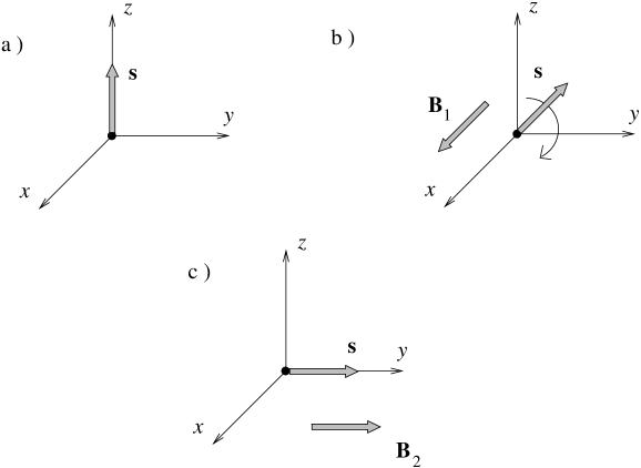
Figure 6: A $z$-polarized electron (fig. a) is placed for a while in a magnetic field ${\bf B}_{1}$ along the $x$-axis causing its spin to precess around the $x$-axis (fig. b); later on a magnetic field ${\bf B}_{2}$ in the $y$-direction is switched on (fig. c). One could also consider an electrically neutral spin 1/2 particle in a potential $\mu{\bf s}\cdot{\bf B}=\mu\epsilon_{ijk}\sigma^{ij}B^{k}\;(i,j,k\in\{1,2,3\})$ where $\mu$ is the gyromagnetic ratio and $\sigma^{ij}$ the spin angular momentum operator.

An explicit calculation by one of us (EK) showed that the interference of the two parts of the beam having experienced the two different magnetic field configurations is the same for a Pin(3,1) beam and for a Pin(1,3) beam.  
 
The explicit calculation consists in comparing the transition amplitudes for Pin (3,1) and Pin (1,3) electrons moving under the conditions described in Fig. 3. The system evolves according to the Dirac equation which reads

$$(i\Gamma^{\alpha}(\partial_{\alpha}+iqA_{\alpha})-m)\psi = 0\;\;\;\mbox{for Pin(1,3) particles}$$

$$(\hat{\Gamma}^{\alpha}(\partial_{\alpha}+iqA_{\alpha})-m)\hat{\psi} = 0\;\;\;\mbox{for Pin (3,1) particles}$$

Since $\hat{\Gamma}^{\alpha}$ may be represented as the matrices $-i\Gamma^{\alpha}$, the equations are the same. Two equivalent initial states under the same evolution remain equivalent throughout all time. Thus, both parts of the beam in the Pin (3,1) case evolve exactly the same way as their respective counterparts in the Pin (1,3) case, the interference patterns produced in either case are identical. The same will hold true for any configuration in which the matter field is required to change continuously.  

Reflection

Since the previous experiment turned out not to give a parity transformation, EK went on to study the interference between two parts of a fermion beam passing through some medium $M$ as shown in fig. 7. The part which follows path 1 is transmitted directly through the medium, whereas the part which follows path 2 is reflected twice before passing through. Such an experiment could be achieved by passing neutrons through a magnetic crystal.  
 
Although the idea of reflection from a surface might bring to mind the idea of parity transformation, the reflections involved here have nothing to do with the parity transformation $\Lambda_{P}$ (or $\hat{\Lambda}_{P}$). In other words, although the neutrons following path 2 are reflected twice, they do not undergo any parity transformations as called for in fig. 5. Hence this setup also fails to realize fig. 5.

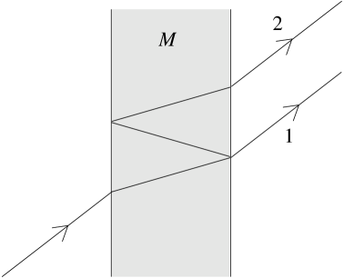
Figure 7: A reflection experiment intended to find a difference between two types of pinors.

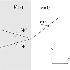
Figure 8: Reflection and transmission of a pinor particle at an interface.

That reflection at a boundary does not produce any parity transformation is best seen by just solving the problem of reflection and transmission of a plane wave between two media, one with a free-particle Dirac Hamiltonian and one with a Hamiltonian consisting of the free-particle part plus a potential $V$, as shown schematically in fig. 8. The solution of this problem can be found in several books [45]. It is done by matching coefficients of solutions and will not bring in any parity transformations; again the requirement of continuity is the stumbling block.  
 
Thus reflection at a boundary cannot be used to distinguish between particles of different Pin groups either.  
 

4.5 Time reversal and Kramers’ degeneracy

In quantum mechanics, if one requires the Hamiltonian to be invariant under time reversal, then the time reversal operator is antiunitary. Indeed the Hamiltonian $H$ generates time evolution:

$$H|\,t\,\rangle=i\partial_{t}\,|\,t\,\rangle\;;$$

$H$ is invariant under time reversal if there exists an antiunitary operator $A_{T}$ such that

$$A_{T}H^{*}A_{T}^{-1}=H$$

with the asterisk denoting complex conjugate; then $A_{T}|\,t\,\rangle^{*}$ satisfies the time reversed equation.  
 
Kramers has shown (see e.g. [115, p. 81] [96, p. 281] or [74, p. 408]; see also [6, p. 601]) that, given an antiunitary time reversal operator $A_{T}$ defined as in eq. (42) with the matrix ${\mathcal{A}}_{T}$ satisfying

$${\mathcal{A}}_{T}{\mathcal{A}}_{T}^{*}=-1{\rm I}$$

and such that it commutes with the Hamiltonian $H$ of the system, an eigenstate $(|n\rangle)$ of $H$ and the time reversed eigenstate $A_{T}(|n\rangle^{*})$ are two different states with the same energy. This degeneracy can be removed by adding an interaction which does not commute with $A_{T}$.  
 
Can Kramers’ theorem provide a method for distinguishing $\Psi$-particles (with $\Lambda^{2}_{T}=1{\rm I}$) from $\hat{\Psi}$-particles (with $\hat{\Lambda}^{2}_{T}=-1{\rm I}$)? We have established the relationship between the time reversal operator ${\mathcal{A}}_{T}$ and the unitary time reversal operator $\Lambda_{T}$ in section 3, namely

$${\mathcal{A}}_{T}{\mathcal{C}}^{-1}=\Lambda_{T}\;.$$

Kramers’ theorem cannot be used to distinguish the two Pin groups (even though $\Lambda_{T}^{2}=1{\rm I}$ and $\hat{\Lambda}_{T}^{2}=-1{\rm I}$):  
 
Let the operators ${\mathcal{A}}_{T}$ and $\hat{{\mathcal{A}}}_{T}$ correspond to $\Lambda_{T}$ and $\hat{\Lambda}_{T}$, respectively.

$$\Lambda_{T}={\mathcal{A}}_{T}{\mathcal{C}}^{-1}\;\qquad\hat{\Lambda}_{T}=\hat{{\mathcal{A}}}_{T}\hat{\mathcal{C}}^{-1}$$

where

$${\mathcal{C}}\Gamma^{*}_{\alpha}{\mathcal{C}}^{-1}=-\Gamma_{\alpha}\quad\mbox{and}\quad\hat{\mathcal{C}}\hat{\Gamma}^{*}_{\alpha}\hat{\mathcal{C}}^{-1}=\hat{\Gamma}_{\alpha}\;.$$

A double time reversal is not produced by ${\mathcal{A}}_{T}^{2}$ but by ${\mathcal{A}}_{T}{\mathcal{A}}^{*}_{T}$ since, according to the defining equation $\psi^{\prime}(Tx)={\mathcal{A}}_{T}\psi^{*}(x)$, and the field operator $\Psi$ transforms according to equation (42) as

$$A_{T}A_{T}\Psi(x)A_{T}^{-1}A_{T}^{-1}=\zeta{\mathcal{A}}_{T}(\zeta{\mathcal{A}}_{T}\Psi^{*}(x))^{*}={\mathcal{A}}_{T}{\mathcal{A}}_{T}^{*}\Psi(x)\;.$$

Whereas $\Lambda^{2}_{T}\neq\hat{\Lambda}^{2}_{T}$, the double antiunitary time reversal shows no such difference:

$${\mathcal{A}}_{T}{\mathcal{A}}_{T}^{*}=\hat{\mathcal{A}}_{T}\hat{\mathcal{A}}_{T}^{*}=-1{\rm I}\;.$$

Both $\Psi$- and $\hat{\Psi}$-particles can be used to construct degenerate time-reversed pairs. It follows that Kramer’s degeneracy cannot be used to distinguish $\Psi$-particles and $\hat{\Psi}$-particles.

4.6 Charge Conjugation; Positronium; Neutrinoless Double Beta Decay

Positronium

Once more, positronium proves to be a useful test bed for discrete symmetries. In Appendix D we briefly review from our perspective the textbook example of how charge conjugation decides the lifetimes of two different positronium states.  

Neutrinoless double beta decay

Double beta decay occurs usually with the emission of two neutrinos. However, if the neutrino associated with a beta decay is reabsorbed to produce a second beta decay, then no neutrino is emitted, and the process is called neutrinoless double beta decay. Diagrams of neutrinoless double beta decay in two different reactions are given in fig. 9 and fig. 10. If the same neutrino is emitted and absorbed, it has to be a particle identical with its antiparticle, i.e. it has to be a Majorana particle. (Recall that a Majorana particle is one for which $\psi^{\rm c}=\psi$). The possible observation of neutrinoless double beta decay has been analyzed by Klapdor-Kleingrothaus [60].  
 
The discussion in section 3.4 indicates that a Majorana particle can only be a Pin(3,1) particle. Thus the existence of Majorana neutrinos, if confirmed, would have some implication for the topology of the universe, namely that the universe is a manifold which can serve as a base for a Pin(3,1)-bundle.

Figure 9: Quark diagram for neutrinoless double beta decay ($2n\to 2p+2e^{-}$ in ${\rm{}^{82}Se}\to{\rm{}^{82}Kr}+2e^{-}$).

Figure 10: We note also another type of neutrinoless double beta decay: Quark diagram for $K^{+}\to\pi^{-}+2e^{+}$.

5 The Pin group in $s$ space, $t$ time dimensions

In order to analyze the properties of the two Pin groups in arbitrary dimensions, we first review and simplify a few topics, treated in detail in [28, 30] and [39]. This section is organized as follows.  

1. The difference between $s+t$ even and $s+t$ odd

2. Chirality

3. Construction of the gamma matrices. Periodicity modulo 8.

4. Conjugate and complex gamma matrices.

5. The short exact sequence $1{\rm I}\rightarrow{\rm Spin}(t,s)\rightarrow{\rm Pin}(t,s)\rightarrow{\mathbb{Z}}_{2}\rightarrow 0$

6. Grassman (superclassical) pinor fields

7. String theory and spin structures

In this section we will use the $P(1)$ parity transformation, which reverses only one axis instead of three.

5.1 The difference between $s+t$ even and $s+t$ odd

In this section $s+t=d=2p$ and $s^{\prime}+t^{\prime}=d+1=2p+1$. In brief:

• $t+s=2p=d$

  • • Only one irreducible faithful representation of the gamma matrices

    • The center of Pin$(t,s)$ is ${\mathbb{R}}^{+}_{\times}1{\rm I}$ (multiples of the unit element)

• $t^{\prime}+s^{\prime}=2p+1=d+1$

  • • Two inequivalent irreducible faithful representations of the gamma matrices

    • The center of Pin$(t^{\prime},s^{\prime})$ is ${\mathbb{R}}^{+}_{\times}1{\rm I}\cup{\mathbb{R}}^{+}_{\times}\Gamma_{d+2}$

    • The map ${\rm Pin}(t^{\prime},s^{\prime})\rightarrow O(t^{\prime},s^{\prime})$ is not surjective

A key element in the proofs of some of the above statements is the construction of the generators for ${\rm Pin}(t^{\prime},s^{\prime})$ given the generators $\{\Gamma_{\alpha}\}$ for ${\rm Pin}(t,s)$.  
 
We begin with $s+t=d=2p$. The algebra over the reals generated by the (possibly complex) $2^{p}\times 2^{p}$ matrices ($\Gamma_{\alpha}$) is a faithful representation of the Clifford algebra ${\mathcal{C}}(t,s)$. This representation is unique, modulo similarity transformations, and irreducible.  
 
The center (set of elements which commute with all elements) of ${\rm Pin}(t,s)$ is ${\mathbb{R}}^{+}_{\times}1{\rm I}$.  
 
We now consider the case $s^{\prime}+t^{\prime}=d+1=2p+1$, with either $s^{\prime}=s+1$ or $t^{\prime}=t+1$. Set

$$\Gamma_{d+1}:=\Gamma_{1}\Gamma_{2}...\Gamma_{d}\qquad\mbox{ and similarly for $\hat{\Gamma}_{d+1}$}\qquad\mbox{($d$ even)}.$$ (48)

We note

$$(\Gamma_{d+1})^{2}=(-1)^{s+p}1{\rm I}_{2^{p}}\;,\qquad(\hat{\Gamma}_{d+1})^{2}=(-1)^{t+p}1{\rm I}_{2^{p}}\;,\qquad d=2p.$$ (49)

We also note that $\Gamma_{d+1}$ anticommutes with all $\Gamma_{\alpha}\in{\rm Pin}(t,s)$, and that a similar statement holds for $\hat{\Gamma}_{d+1}$. Therefore we can use $k\Gamma_{d+1}$, where $k$ is a phase, to construct a basis for ${\rm Pin}(t+1,s)$ and for ${\rm Pin}(t,s+1)$ as follows; similar construction of ${\rm Pin}(s+1,t)$ and of ${\rm Pin}(s,t+1)$ can be done using $\hat{\Gamma}_{d+1}$.  
 
For

$$k^{2}=(-1)^{s+p},\qquad(k\Gamma_{d+1})^{2}=1{\rm I}$$ (50)

the set of anticommuting matrices $\{\Gamma_{\alpha},k\Gamma_{d+1}\}$ generates ${\rm Pin}(t+1,s)$. The two choices $k=\pm(-1)^{(s+p)/2}$ provide two inequivalent representations of the group ${\rm Pin}(t+1,s)$.  
 
For

$$k^{2}=(-1)^{s+p+1},\qquad(k\Gamma_{d+1})^{2}=-1{\rm I}$$ (51)

the set of anticommuting matrices $\{\Gamma_{\alpha},k\Gamma_{d+1}\}$ generates ${\rm Pin}(t,s+1)$. The two choices $k=\pm i(-1)^{(s+p)/2}$ provide two inequivalent representations of ${\rm Pin}(t,s+1)$. Similar results hold for ${\rm Pin}(s+1,t)$ and ${\rm Pin}(s,t+1)$.  
 
For $s^{\prime}+t^{\prime}$ odd, the center of ${\rm Pin}(t^{\prime},s^{\prime})$ consists of ${\mathbb{R}}^{+}_{\times}1{\rm I}$ and ${\mathbb{R}}^{+}_{\times}\Gamma_{d+2}$. Indeed the product

$$\Gamma_{d+2}=\Gamma_{1}\Gamma_{2}...\Gamma_{d}\Gamma_{d+1}\qquad\mbox{with}\qquad\Gamma_{d+1}=\Gamma_{1}\Gamma_{2}...\Gamma_{d}$$ (52)

commutes with all elements in $\{\Gamma_{\alpha},\Gamma_{d+1}\}$.  
 
For $s^{\prime}+t^{\prime}$ odd, the map ${\rm Pin}(t^{\prime},s^{\prime})\rightarrow O(t^{\prime},s^{\prime})$ is not surjective. Namely, there is no element in ${\rm Pin}(t^{\prime},s^{\prime})$ which maps into the element of $O(t^{\prime},s^{\prime})$ which reverses the axes. Indeed let $(PT)={\rm diag}(-1,...-1)$, then there is no $\Lambda_{PT}$ satisfying

$$\Lambda_{PT}\Gamma_{\alpha}\Lambda_{PT}^{-1}=\Gamma_{\beta}{(PT)^{\beta}}_{\alpha}=-\Gamma_{\alpha}\;,\qquad\mbox{for all $\Gamma_{\alpha}$}$$ (53)

since this would imply

$$\Lambda_{PT}\Gamma_{d+2}+\Gamma_{d+2}\Lambda_{PT}=0\;,$$

but $\Gamma_{d+2}$ commutes with all elements in ${\rm Pin}(t^{\prime},s^{\prime})$, and $\Lambda_{PT}\Gamma_{d+2}\neq 0$ since $\Lambda_{PT}$ and $\Gamma_{d+2}$ are invertible.

The twisted map

To eliminate some of the differences between $d$ odd and $d$ even, one can introduce a map, sometimes called the twisted map,

$$\tilde{\mathcal{H}}:{\rm Pin}(t,s)\rightarrow O(t,s)\;,$$

surjective in all dimensions, as follows. The Clifford algebra is a graded algebra

$${\mathcal{C}}(t,s)={\mathcal{C}}_{+}(t,s)+{\mathcal{C}}_{-}(t,s)$$ (54)

where ${\mathcal{C}}_{+}$ is generated by even products of elements of the basis, and ${\mathcal{C}}_{-}$ is generated by odd products. Let

$$\begin{array}[]{cccl}\alpha(\Lambda_{+})&=&\Lambda_{+}&\qquad\mbox{ for }\Lambda_{+}\in{\mathcal{C}}_{+}(t,s)\\ \alpha(\Lambda_{-})&=&-\Lambda_{-}&\qquad\mbox{ for }\Lambda_{-}\in{\mathcal{C}}_{-}(t,s)\end{array}$$ (55)

The map $\tilde{\mathcal{H}}$, defined by

$$\alpha(\Lambda_{L})\Gamma_{\alpha}\Lambda_{L}^{-1}=\Gamma_{\beta}{L^{\beta}}_{\alpha}$$ (56)

is surjective in all dimensions.  
 
We note also that $\tilde{{\mathcal{H}}}(\Gamma_{\alpha})$ reverses the $\alpha$-axis. The twisted map $\tilde{\mathcal{H}}$ seems desirable, but eq. (56) is not a similarity transformation and the invariance of the Dirac equation under Lorentz transformations requires the similarity transformation $\Lambda_{L}\Gamma_{\alpha}\Lambda^{-1}=\Gamma_{\beta}{L^{\beta}}_{\alpha}$. Attempts to find maps [58]

$$\rho:{\rm Pin}(t,s)\rightarrow{\rm Pin}(t,s)$$

to recover a similarity transformation, i.e. $\rho$ such that

$$\alpha(\Lambda_{L})\Gamma_{\alpha}\Lambda^{-1}_{L}=\rho(\Lambda){\Gamma_{\alpha}}(\rho(\Lambda))^{-1}\;,$$

obviously fail in odd dimensions, and are very awkward in even dimensions. We shall not work with the twisted map.

5.2 Chirality

In this paragraph the matrix $\Gamma_{d+1}=\Gamma_{1}\Gamma_{2}...\Gamma_{d}$ is used to define chirality for $d$ even.

$\Gamma_{d+1}$ is a linear operator on the space $S$ of spinors. We recall

$$(\Gamma_{d+1})^{2}=(-1)^{s+p}1{\rm I}_{2^{p}}\;,\qquad(\hat{\Gamma}_{d+1})^{2}=(-1)^{t+p}1{\rm I}_{2^{p}}\;.$$ (57)

The eigenvalue equation

$$\Gamma_{d+1}\psi=\alpha\psi$$

implies

$$(\Gamma_{d+1})^{2}\psi=\alpha^{2}\psi=(-1)^{s+p}\psi\qquad\mbox{ by (\ref{eq:gamma2}) }$$

hence

$$\alpha^{2}=(-1)^{s+p}\;.$$

Thus

$$\alpha = \pm 1\qquad\mbox{ if $s+p$ is even}$$

$$\alpha = \pm i\qquad\mbox{ if $s+p$ is odd (as in section \ref{sec:pinreps})}$$

One denotes by $S_{+}$ the eigenspace with eigenvalue 1 or $i$, and by $S_{-}$ the eigenspace with eigenvalue $-1$ or $-i$.

$$S=S_{+}\oplus S_{-}$$

Therefore the projection matrices

$${\mathcal{P}}_{\pm}=\left\{\begin{array}[]{ll}{\scriptstyle{1\over 2}}(1{\rm I}_{2^{p}}\pm\Gamma_{d+1})\;,&\mbox{$s+p$ even}\\ {\scriptstyle{1\over 2}}(1{\rm I}_{2^{p}}\pm i\Gamma_{d+1})\;,&\mbox{$s+p$ odd}\end{array}\right.$$ (58)

project a $2^{p}$-component pinor into two $2^{p-1}$-component spinors.  
 
$\Gamma_{d+1}$ for $s+p$ even, and $i\Gamma_{d+1}$ for $s+p$ odd, are called chirality operators.  
 
A chiral basis is a basis adapted to the splitting $S=S_{+}\oplus S_{-}$. In a chiral basis

$$\Gamma_{d+1}=\left(\begin{array}[]{cc}-1{\rm I}_{2^{p-1}}&0\\ 0&1{\rm I}_{2^{p-1}}\end{array}\right)\;.$$

Polchinski [88, app. B] gives a recursion construction of a chiral basis in terms of the Pauli matrices $\{\sigma_{i}\}$.  
 
Remark: For $s+t$ even, $\Gamma_{\alpha}\Gamma_{d+1}=-\Gamma_{\alpha}\Gamma_{d+1}$, hence the matrix $\Gamma_{d+1}$ is a solution $\Lambda_{L}$ of

$$\Lambda_{L}\Gamma_{\alpha}\Lambda_{L}^{-1}=-\Gamma_{\alpha}$$

which implies $(L)={\rm diag}(-1,...,-1)$. Since the dimension of space-time is even, this Lorentz transformation does not change the handedness of the system of coordinates.  

5.3 Construction of gamma matrices. Periodicity modulo 8.

Two useful mathematical references are the books by Gilbert and Murray [48] and by Porteous [89].  
 
The study of ${\rm Pin}(t,s)$ for arbitrary $t$ and $s$ is considerably simplified by the fact that the groups depend not on $s$ and $t$ but on $|s-t|$ modulo 8. Moreover, ${\rm Pin}(t,s)$ and ${\rm Pin}(s,t)$ are isomorphic for $|s-t|=0$ modulo 4.  
 
The proof uses the isomorphism

$$M_{4}({\mathbb{R}})\simeq{{\mathbb{H}}}\otimes_{\mathbb{R}}{{\mathbb{H}}}$$ (59)

where $M_{4}({\mathbb{R}})$ is the algebra of real $4\times 4$ matrices and ${{\mathbb{H}}}$ the quaternion algebra. This isomorphism is not trivial. It has been questioned on the grounds that the left hand side is real and the right hand side seems to be complex, given that a well known two-dimensional representation of the quaternion basis consists of the matrix $1{\rm I}_{2}$ together with $i$ times the Pauli matrices which cannot be all imaginary. This argument for the complexity of the quaternion algebra is obviously meaningless since complex representations of real algebras abound, as can be seen, for instance, in this paper. We prove the isomorphism in appendix B because it is not easily available to non-specialists.  
 
In paragraph 5.1, we constructed ${\rm Pin}(t+1,s)$ and ${\rm Pin}(t,s+1)$ by adding $k\Gamma_{d+1}$, with different values of $k^{2}$, to the basis of ${\rm Pin}(t,s)$ with $t+s=d=2p$. Now we combine $t+s=2p$ and $t^{\prime}+s^{\prime}=d^{\prime}$ arbitrary. By tensoring the Clifford algebras ${\mathcal{C}}(t,s)$ and ${\mathcal{C}}(t^{\prime},s^{\prime})$ one can obtain either one of the two Clifford algebras ${\mathcal{C}}(t+t^{\prime},s+s^{\prime})$ or ${\mathcal{C}}(t+s^{\prime},s+t^{\prime})$, depending on the sign of $k^{2}$ in $k\Gamma_{d+1}$.

$${\mathcal{C}}(t,s)\otimes_{k}{\mathcal{C}}(t^{\prime},s^{\prime}) = {\mathcal{C}}(t+t^{\prime},s+s^{\prime})\qquad\mbox{for }k^{2}=1$$ (60)

$${\mathcal{C}}(t,s)\otimes_{k}{\mathcal{C}}(t^{\prime},s^{\prime}) = {\mathcal{C}}(t+s^{\prime},s+t^{\prime})\qquad\mbox{for }k^{2}=-1$$ (61)

Let $\{1{\rm I},\Gamma_{\alpha}\}$ be a basis of ${\mathcal{C}}(t,s)$ and $\{1{\rm I}^{\prime},\Gamma_{\alpha^{\prime}}\}$ be a basis of ${\mathcal{C}}(t^{\prime},s^{\prime})$, then the $d+d^{\prime}$ elements $\{\Gamma_{\alpha}\otimes 1{\rm I}^{\prime},k\Gamma_{d+1}\otimes\Gamma_{\alpha^{\prime}}\}$ form a basis for their tensor product. Henceforth we abbreviate $\otimes_{k}$ to $\otimes$.  
 
Proof: Since $\Gamma_{\alpha}$ anticommutes with $\Gamma_{d+1}$, the elements in this basis anticommute pairwise. Their squares are

$$(\Gamma_{\alpha}\otimes 1{\rm I}^{\prime})^{2} = (\Gamma_{\alpha})^{2}\otimes 1{\rm I}^{\prime}=(1{\rm I}\otimes 1{\rm I}^{\prime})\eta_{\alpha\alpha}$$

$$(k\Gamma_{d+1}\otimes\Gamma_{\alpha^{\prime}})^{2} = k^{2}(1{\rm I}\otimes 1{\rm I}^{\prime})\eta_{\alpha^{\prime}\alpha^{\prime}}\;;$$

the sign of $k^{2}$ determines the combination $t+t^{\prime}$ or $t+s^{\prime}$ in the tensor product ${\mathcal{C}}(t,s)\otimes{\mathcal{C}}(t^{\prime},s^{\prime})$. $\Box$ 
 
 
In order to prove the periodicity of the Clifford algebra modulo 8, we prove

$${\mathcal{C}}(0,s+8) \simeq M_{16}({\mathbb{R}})\otimes{\mathcal{C}}(0,s)$$ (62)

$${\mathcal{C}}(t,s) \simeq M_{2^{t}}({\mathbb{R}})\otimes{\mathcal{C}}(0,s-t)\qquad\mbox{for $s>t$}$$ (63)

When tensoring Clifford algebras we can use either (60) or (61). Using (60) is easier but using (61) brings out interesting results. In brief, if we use (60)

$${\mathcal{C}}(0,s+8) \simeq {\mathcal{C}}(0,2)\otimes{\mathcal{C}}(0,s+6)$$

$$\simeq \left(\otimes{\mathcal{C}}(0,2)\right)^{4}\otimes{\mathcal{C}}(0,s)$$

$$\simeq M_{16}({\mathbb{R}})\otimes{\mathcal{C}}(0,s)\qquad\qquad\mbox{since ${\mathcal{C}}(0,2)\simeq M_{2}({\mathbb{R}})$}$$

But if we use (61) we bring out the quaternionic algebras since ${\mathcal{C}}(2,0)$ is isomorphic to ${{\mathbb{H}}}$; we have then enough information to construct the classification table. Using (61) we obtain

$${\mathcal{C}}(0,s+8) \simeq {\mathcal{C}}(0,2)\otimes{\mathcal{C}}(s+6,0)$$

$$\simeq {\mathcal{C}}(0,2)\otimes{{\mathbb{H}}}\otimes{\mathcal{C}}(0,s+4)\simeq\ldots$$

$$\simeq M_{2}({\mathbb{R}})\otimes{{\mathbb{H}}}\otimes M_{2}({\mathbb{R}})\otimes{{\mathbb{H}}}\otimes{\mathcal{C}}(0,s)$$

The proof of (63) is analogous. With $k^{2}=1$,

$${\mathcal{C}}(t,s) \simeq (\otimes{\mathcal{C}}(1,1))^{t}\otimes{\mathcal{C}}(0,s-t)$$

$$= M_{2^{t}}({\mathbb{R}})\otimes{\mathcal{C}}(0,s-t)\;.$$

Example: Constructing gamma matrices from Pauli matrices.

$$\sigma_{1}=\left(\begin{array}[]{cc}\;0&\;1\\ 1&0\end{array}\right)\;,\quad\sigma_{2}=\left(\begin{array}[]{cc}\;0&-i\\ i&0\end{array}\right)\;,\quad\sigma_{3}=\left(\begin{array}[]{cc}\;1&0\\ 0&-1\end{array}\right)\;,\quad$$

$$\sigma_{j}\sigma_{k}=i\epsilon_{jkl}\sigma_{l}\;,\qquad(\sigma_{i})^{2}=1{\rm I}_{2}\;,\qquad\sigma_{1}\sigma_{2}\sigma_{3}=i1{\rm I}_{2}\;.$$

In dimensions 2 and 3, the gamma matrices are $2\times 2$ matrices and we can write down table 2. Let a matrix in ${\mathcal{C}}$ be written $M=m^{0}1{\rm I}+m^{i}\Gamma_{i}+m^{ij}\Gamma_{i}\Gamma_{j}+m\Gamma_{1}\Gamma_{2}\cdots\Gamma_{d}$ ; $M$ is an element of a real vector space; the isomorphism in the last column is dictated by the properties of the vector space basis.

$$\begin{array}[]{|c|c|c|c|c|}\hline\cr\mbox{Clifford alg.}&\mbox{alg. generators}&\mbox{vector space basis}&\,{\rm dim}_{{\mathbb{R}}}&\mbox{isomorphism}\\ \hline\cr\hline\cr{\mathcal{C}}(0,1)&1,i&1,i&2&{\mathbb{C}}\\ \hline\cr{\mathcal{C}}(1,0)&1,1^{\prime}&1,1^{\prime}&2&{\mathbb{R}}\oplus{\mathbb{R}}\\ \hline\cr\hline\cr{\mathcal{C}}(0,2)&1{\rm I}_{2},i\sigma_{1},i\sigma_{3}&1{\rm I}_{2},i\sigma_{1},i\sigma_{2},i\sigma_{3}&4&{\mathbb{H}}\\ \hline\cr{\mathcal{C}}(1,1)&1{\rm I}_{2},(\sigma_{1}\mbox{ or }\sigma_{3}),i\sigma_{2}&1{\rm I}_{2},\sigma_{1},i\sigma_{2},\sigma_{3}&4&M_{2}({\mathbb{R}})\\ \hline\cr{\mathcal{C}}(2,0)&1{\rm I}_{2},\sigma_{1},\sigma_{3}&1{\rm I}_{2},\sigma_{1},i\sigma_{2},\sigma_{3}&4&M_{2}({\mathbb{R}})\\ \hline\cr\hline\cr{\mathcal{C}}(0,3)&1{\rm I}_{2},i\sigma_{1},i\sigma_{2},i\sigma_{3}&1{\rm I}_{2}+7\mbox{ matrices}&8&{\mathbb{H}}\oplus{\mathbb{H}}\\ \hline\cr{\mathcal{C}}(1,2)&1{\rm I}_{2},\sigma_{2},i\sigma_{1},i\sigma_{3}&1{\rm I}_{2}+7\mbox{ matrices}&8&{\mathbb{H}}\otimes{\mathbb{C}}\\ \hline\cr{\mathcal{C}}(2,1)&1{\rm I}_{2},\sigma_{1},\sigma_{3},i\sigma_{2}&1{\rm I}_{2}+7\mbox{ matrices}&8&M_{2}({\mathbb{R}})\oplus M_{2}({\mathbb{R}})\\ \hline\cr{\mathcal{C}}(3,0)&1{\rm I}_{2},\sigma_{1},\sigma_{2},\sigma_{3}&1{\rm I}_{2}+7\mbox{ matrices}&8&M_{2}({\mathbb{C}})\\ \hline\cr\end{array}$$

Table 2: Gamma matrices in 1,2 and 3 dimensions.

In dimensions higher than 3, equations (60) and (61) can be used for constructing gamma matrices. We work out ${\mathcal{C}}(1,3)$ and ${\mathcal{C}}(3,1)$ explicitly:

• ${\mathcal{C}}(1,3)\simeq{\mathcal{C}}(1,1)\otimes{\mathcal{C}}(0,2)$ for $k^{2}=1$, $k=\pm 1$

  • the algebra generators are: $\sigma_{1}\otimes 1{\rm I}_{2}$, $i\sigma_{2}\otimes 1{\rm I}_{2},-k\sigma_{3}\otimes(i\sigma_{1})$, $-k\sigma_{3}\otimes(i\sigma_{2})$
    consist of 3 real matrices, and 1 imaginary one.

• ${\mathcal{C}}(1,3)\simeq{\mathcal{C}}(1,1)\otimes{\mathcal{C}}(2,0)$ for $k^{2}=-1$, $k=\pm i$

  • the algebra generators are: $\sigma_{1}\otimes 1{\rm I}_{2}$, $i\sigma_{2}\otimes 1{\rm I}_{2},-k\sigma_{3}\otimes\sigma_{1}$, $-k\sigma_{3}\otimes\sigma_{3}$
    consist of 2 real matrices, and 2 imaginary ones.

• ${\mathcal{C}}(3,1)\simeq{\mathcal{C}}(1,1)\otimes{\mathcal{C}}(2,0)$ for $k^{2}=1$, $k=\pm 1$

  • Changing the value of $k$ in the previous basis yields 4 real matrices. This is a Majorana representation.

• ${\mathcal{C}}(3,1)\simeq{\mathcal{C}}(1,1)\otimes{\mathcal{C}}(0,2)$ for $k^{2}=-1$, $k=\pm i$

  • Changing the value of $k$ in the first basis yields 3 real matrices, and 1 imaginary one.

${\mathcal{C}}(1,3)$ does not admit a real representation; ${\mathcal{C}}(3,1)$ does admit a real representation.  
 
In section 3.1, the label $t$ for time is equal to 1 and the label $s$ for space is equal to 3, therefore ${\mathcal{C}}(t,s)$ signals at a glance a metric of signature $(+,-,-,-)$ and ${\mathcal{C}}(s,t)$ a metric of signature $(+,+,+,-)$. Here $t$ and $s$ are arbitrary, and we shall use $(m,n)$ rather than $(t,s)$. Table 3 lists the algebra isomorphisms of ${\mathcal{C}}(m,n)$ with $d=m+n$ for all possible values of $(m-n)$ mod 8. The vector space $M_{k}({\mathbb{R}})$ of $k\times k$ real matrices is abbreviated to ${\mathbb{R}}(k)$ and the space of $k\times k$ quaternionic matrices (the matrix elements are quaternions) is denoted ${\mathbb{H}}(k)$. For example the isomorphism

$$M_{4}({\mathbb{R}})\simeq{\mathbb{H}}\otimes{\mathbb{H}}\quad\mbox{ is abbreviated }\quad{\mathbb{R}}(4)\simeq{\mathbb{H}}(2)\;.$$

$$\begin{array}[]{|c|c|c|c|c|}\hline\cr(m-n)\,{\rm mod}\,8&0&1&2&3\\ \hline\cr{\mathcal{C}}(m,n)&{\mathbb{R}}(2^{d/2})&{\mathbb{R}}(2^{(d-1)/2})\oplus{\mathbb{R}}(2^{(d-1)/2})&{\mathbb{R}}(2^{d/2})&{\mathbb{C}}(2^{(d-1)/2})\\ \hline\cr\hline\cr(m-n)\,{\rm mod}\,8&4&5&6&7\\ \hline\cr{\mathcal{C}}(m,n)&{{\mathbb{H}}}(2^{d/2-1})&{{\mathbb{H}}}(2^{(d-1)/2-1})\oplus{{\mathbb{H}}}(2^{(d-1)/2-1})&{{\mathbb{H}}}(2^{d/2-1})&{\mathbb{C}}(2^{(d-1)/2})\\ \hline\cr\end{array}$$

Table 3: Algebra isomorphisms

This table is valid for both $m-n>0$ and $m-n<0$ since a negative number modulo 8 is equal to a positive number.  
 
Given $\hat{\Gamma}\in{\mathcal{C}}(m,n)$, $m>n$, and $\Gamma\in{\mathcal{C}}(m,n)$, $m<n$, one can use $\hat{\Gamma}=i\Gamma$ for verifying, for instance, ${\mathcal{C}}(0,5)$ given ${\mathcal{C}}(5,0)={\mathbb{H}}(2)\oplus{\mathbb{H}}(2)$; one finds ${\mathcal{C}}(0,5)={\mathbb{H}}(2)\oplus i{\mathbb{H}}(2)={\mathbb{H}}(2)\otimes{\mathbb{C}}$. Now ${\mathbb{H}}\otimes{\mathbb{C}}\simeq{\mathbb{C}}(2)$, so ${\mathcal{C}}(0,5)\simeq{\mathbb{C}}(4)$ which is correct for $-5=3$ mod 8.  
 
From table 3 we conclude the following:

• For $d$ even, the vector space isomorphisms are either with vector spaces of real matrices, or vector spaces of quaternionic matrices.

• For $n=1$, ${\mathcal{C}}(m,1)$ admits a real representation for

  $$m = 1,2,3\mbox{ mod }8$$

  $${\rm i.e.}\quad d = 2,3,4,10,11,12\mbox{ etc.}$$

• If ${\mathcal{C}}(m,1)$ admits a real representation, ${\mathcal{C}}(1,m)$ admits a purely imaginary one.

• ${\mathcal{C}}(m,n)$ and ${\mathcal{C}}(n,m)$ are not isomorphic unless $m-n=0$ mod 4.

Another technique for identifying the dimensions which admit real representations consists in assuming all the $\Gamma_{\alpha}$’s real, and seeing if it leads to a contradiction. For instance, let $d=4$, and assume $\Gamma_{1}$, $\Gamma_{2}$, $\Gamma_{3}$, $\Gamma_{4}$ to be real, with $(\Gamma_{j})^{2}=1{\rm I}$, $j\in\{1,2,3\}$ and $(\Gamma_{4})^{2}=-1{\rm I}$. The $\Gamma_{j}$ are symmetric, and $\Gamma_{4}$ is antisymmetric. The algebra generated by the $\Gamma_{\alpha}$’s consists of

• 10 symmetric matrices: $1{\rm I}$, $\Gamma_{j}$, $\Gamma_{4}\Gamma_{j}$, $\Gamma_{4}\Gamma_{j}\Gamma_{k}$

• 6 antisymmetric matrices: $\Gamma_{4}$, $\Gamma_{j}\Gamma_{k}$, $\Gamma_{j}\Gamma_{k}\Gamma_{l}$, $\Gamma_{1}\Gamma_{2}\Gamma_{3}\Gamma_{4}$

These 16 matrices make a basis for $M_{4}({\mathbb{R}})$. There is no contradiction in having assumed the $\Gamma_{\alpha}$’s to be real.  

Onsager construction of gamma matrices

In the proof of (62) and (63) we have given a construction for a basis of ${\mathcal{C}}(t+t^{\prime},s+s^{\prime})$ and ${\mathcal{C}}(t+s^{\prime},s+t^{\prime})$ given a basis for ${\mathcal{C}}(t,s)$ and ${\mathcal{C}}(t^{\prime},s^{\prime})$. It is worth mentioning another construction using the Onsager solution of the Ising model [83]; the explicit representation using this construction can be found in [39]. In particular, one sees by inspection which matrices are real, and which are imaginary both for $d$ even and $d$ odd.  

Majorana pinors, Weyl-Majorana spinors

A pinor is said to be Majorana if it is real (or purely imaginary). If a space $S$ of Majorana pinors is of even dimension, it can be split into two eigenspaces of a chirality operator

$$S=S_{+}\oplus S_{-}\;,$$

then each eigenspace is a space of Weyl-Majorana spinors.  
 
Majorana pinors have been used to avoid confusion in charge conjugation. When a real representation is not available, one replaces a $d$-dimensional complex pinor $\psi=\psi_{1}+i\psi_{2}$ by a $2d$-dimensional real pinor

$$\psi=\left(\begin{array}[]{c}\psi_{1}\\ \psi_{2}\end{array}\right)\qquad\mbox{and}\qquad\psi^{*}=\left(\begin{array}[]{cc}\;1{\rm I}&0\\ 0&-1{\rm I}\end{array}\right)\psi\;.$$

The $2d$-dimensional representation is reducible.

5.4 Conjugate and complex gamma matrices

The set of hermitian conjugate matrices $\{\pm\Gamma_{\alpha}^{\dagger}\}$, the set of inverse matrices $\{\pm\Gamma_{\alpha}^{-1}\}$ and the set of complex conjugate matrices $\{\Gamma_{\alpha}^{*}\}$ obey the same algebra as the set $\{\pm\Gamma_{\alpha}\}$ and the same normalization $\Gamma_{\alpha}\Gamma_{\alpha}^{\dagger}=\pm 1{\rm I}$ (no summation).  
 
For $d$ even there is only one irreducible faithful representation of the gamma matrices of dimension $2^{d/2}$. Hence there are similarity transformations

$$\begin{array}[]{rcll}{\mathcal{H}}^{-1}_{\pm}\Gamma^{\dagger}_{\alpha}{\mathcal{H}}_{\pm}&=&\pm\Gamma_{\alpha}&\mbox{($\Gamma_{\alpha}^{\dagger}$ operates on bras) \qquad(a)}\\ {\mathcal{C}}_{\pm}\Gamma^{*}_{\alpha}{\mathcal{C}}^{-1}_{\pm}&=&\pm\Gamma_{\alpha}&\mbox{($\Gamma_{\alpha}^{*}$ operates on kets) \qquad(b)}\end{array}$$ (64)

We shall not need the similarity transformation of inverse matrices.  
 
Remark: The similarity transformation on $\{\Gamma_{\alpha}^{\dagger}\}$ does not imply that there is a similarity transformation on products $\Gamma_{\alpha}^{\dagger}\Gamma_{\beta}^{\dagger}$. Indeed ${\mathcal{H}}^{-1}(\Gamma_{\alpha}\Gamma_{\beta})^{\dagger}{\mathcal{H}}={\mathcal{H}}^{-1}(\Gamma_{\beta}^{\dagger}\Gamma_{\alpha}^{\dagger}){\mathcal{H}}=\Gamma_{\beta}\Gamma_{\alpha}\neq\Gamma_{\alpha}\Gamma_{\beta}$. This explains the factor $a(\Lambda)$ in the definition of copinor in 3.3.  
 
For $d=2p+1$ odd there are two inequivalent irreducible faithful representations of the gamma matrices of dimension $2^{(d-1)/2}$; hence there may not exist matrices ${\mathcal{H}}_{\pm}$ and ${\mathcal{C}}_{\pm}$ satisfying those similarity transformations — in other words, we could have

$${\mathcal{H}}^{-1}_{\pm}\Gamma^{\dagger}_{\alpha}{\mathcal{H}}_{\pm}=(-1)^{\alpha}\Gamma_{\alpha}\quad\mbox{where}\quad(-1)^{\alpha}=\left\{\begin{array}[]{ll}1&\mbox{for $\alpha=0$}\\ 0&\mbox{for $\alpha\in\{1,2,3\}$}\end{array}\right.$$ (65)

In section 5.1 we gave a construction for a basis of ${\rm Pin}(t^{\prime},s^{\prime})$, $t^{\prime}+s^{\prime}=2p+1$, given a basis of ${\rm Pin}(t,s)$, $t+s=2p$. In this construction the first $2p$ elements were the same as in ${\rm Pin}(t,s)$, hence they satisfy (64a) or (64b) as the case may be. We need to check only which equation is satisfied by the new element $k\Gamma_{d+1}$, or $\hat{k}\hat{\Gamma}_{d+1}$.  
 
We recall (57) the properties of $\Gamma_{d+1}$ and $\hat{\Gamma}_{d+1}$: for $d=2p$, $\Gamma_{d+1}:=\Gamma_{1}\Gamma_{2}\ldots\Gamma_{d}$ and similarly for $\hat{\Gamma}_{d+1}$,

$$\Gamma_{d+1}^{2}=(-1)^{s+p}1{\rm I}_{2^{p}}\;,\qquad\hat{\Gamma}^{2}_{d+1}=(-1)^{t+p}1{\rm I}_{2^{p}}$$

The square of the new element, $(k\Gamma_{d+1})^{2}$, tells us which group we generate (table 4).

$$\begin{array}[]{|r|c|r|r|}\hline\cr\;(k\Gamma_{d+1})^{2}&\mbox{Group}&k^{2}&k\\ \hline\cr\hline\cr 1{\rm I}&\;{\rm Pin}(t+1,s)&(-1)^{s+p}&\pm(-1)^{(s+p)/2}\\ \hline\cr-1{\rm I}&{\rm Pin}(t,s+1)&-(-1)^{s+p}&\pm i\,(-1)^{(s+p)/2}\\ \hline\cr\end{array}$$

Table 4: Constructing a Pin group in odd dimensions.

The two choices for $k$ in their respective groups correspond to two different representations. We calculate the transformation under (64a) and (64b) of the new element $k\Gamma_{d+1}$:

$${\mathcal{H}}_{\pm}^{-1}(k\Gamma_{d+1}){\mathcal{H}}_{\pm} = (-1)^{t}\,\Gamma_{d+1}^{\dagger}$$

$${\mathcal{C}}_{\pm}(k\Gamma_{d+1}){\mathcal{C}}^{-1}_{\pm} = \left\{\begin{array}[]{rl}\Gamma_{d+1}^{*}&\mbox{if $k^{*}=k$}\\ -\Gamma_{d+1}^{*}&\mbox{if $k^{*}=-k$}\\ \end{array}\right.$$

From this, and the requirement that (64a) and (64b) extend to $\Gamma_{d+1}$, we read off

• if $t$ is even, the only choice is ${\mathcal{H}}_{+}$

• if $t$ is odd, in particular if $t=1$, the only choice is ${\mathcal{H}}_{-}$

• if $s-t+1$ mod $4=2$, the only choice is ${\mathcal{C}}_{+}$

• if $s-t+1$ mod $4=0$, the only choice is ${\mathcal{C}}_{-}$

For the corresponding ${\rm Pin}(t,s)$ transformations one finds

$$\hat{\mathcal{H}}_{\pm}={\mathcal{H}}_{\mp}\quad\mbox{and}\quad\hat{\mathcal{C}}_{\pm}={\mathcal{C}}_{\mp}$$

The details of this calculation can be found in [39], as well as properties of ${\mathcal{H}}$ and ${\mathcal{C}}$.

5.5 The short exact sequence $1{\rm I}\rightarrow$ Spin$(t,s)\rightarrow$ Pin$(t,s)\rightarrow{\mathbb{Z}}_{2}\rightarrow 0$

We shall prove that a Pin group is a semidirect product of a Spin group with ${\mathbb{Z}}_{2}$, the group consisting of two elements $\{e,z\}$, where $z^{2}=e$ :

$${\rm Pin}(t,s) = {\rm Spin}(t,s)\ltimes{\mathbb{Z}}_{2}\qquad s+t>1$$

$${\rm Pin}(s,t) = {\rm Spin}(s,t)\ltimes{\mathbb{Z}}_{2}\qquad s+t>1$$

where $\ltimes$ is defined below. Spin$(t,s)$ and Spin$(s,t)$ are isomorphic, but a semidirect product “scrambles” the elements of its components and, as we know, Pin$(t,s)$ is not necessarily isomorphic to Pin$(s,t)$. As we have shown in 5.3, they are isomorphic only when $s-t=0$ mod 4. The semidirect product construction does not work for Pin(0,1), since ${\mathbb{Z}}_{2}\ltimes{\mathbb{Z}}_{2}={\mathbb{Z}}_{2}\times{\mathbb{Z}}_{2}$.
 
a) First we prove general properties of semidirect products, then we apply them to Spin and Pin. Let

$$G = H\ltimes{\mathbb{Z}}_{2}$$

$$\hat{G} = \hat{H}\ltimes{\mathbb{Z}}_{2}$$

where there is an isomorphism $\phi:H\rightarrow\hat{H}$.  
 
Let $t:({\mathbb{Z}}_{2}\times H)\rightarrow H$ be an element of the group of automorphisms of $H$ indexed by ${\mathbb{Z}}_{2}$.

$$t_{z}:H\rightarrow H\qquad\mbox{ by }\qquad h\mapsto t_{z}(h)=t(z,h)=zhz^{-1}\;.$$

Note that $z$ is not in $H$ but acts multiplicatively on $H$. The semidirect product $G=H\ltimes{\mathbb{Z}}_{2}$ is the space of ordered pairs $(h,z)$ and $(h,e)$, $h\in H$ with the product law

$$(h_{1},z_{1})\cdot(h_{2},z_{2})=(h_{1}t(z_{1},h_{2}),z_{1}z_{2})\;;$$

here $z_{i}$, $i=1,2$, is either $e$ or $z$; when working with ${\mathbb{Z}}_{2}$, it is difficult to be correct without being pedantic.  
 
If ${\mathbb{Z}}_{2}$ and $H$ commute, $t(z_{i},h)=h$ and the semidirect product becomes a direct product. As the simplest example of semidirect product scrambling, compare (see section 3.2 and also appendix C)

$${\mathbb{Z}}_{3}\times{\mathbb{Z}}_{2}\qquad\mbox{ and }\qquad{\mathbb{Z}}_{3}\ltimes{\mathbb{Z}}_{2}=D_{3}$$

where the dihedral group $D_{3}$ is the group of symmetries of a regular triangle.  
 
Consider the short exact sequence

$$1{\rm I}\rightarrow{\rm Spin}(t,s)\rightarrow{\rm Pin}(t,s)\rightarrow{\mathbb{Z}}_{2}\rightarrow 0\;.$$

We shall show that

	if $s+t$ is odd,	$O(s,t)=SO(s,t)\times{\mathbb{Z}}_{2}$
	if $s+t$ is even,	$O(s,t)=SO(s,t)\ltimes{\mathbb{Z}}_{2}$

Since a direct product is a special case of a semidirect product, we begin with

$$(a,z_{i})\in SO(s,t)\ltimes{\mathbb{Z}}_{2}$$

The identification $(a_{i},z_{i})$ with $a_{i}z_{i}=:g_{i}\in O(s,t)$ makes sense because $z_{i}$ is not necessarily in $SO(s,t)$, and because it makes the definition of the semidirect product consistent with the group product in $O(s,t)$. Indeed

$$(a_{1},z_{1})\cdot(a_{2},z_{2}) = (a_{1}z_{1}a_{2}z_{1}^{-1},z_{1}z_{2})$$

$$\simeq a_{1}z_{1}a_{2}z_{1}^{-1}z_{1}z_{2}=g_{1}g_{2}\;.$$

The difference between $s+t$ odd and $s+t$ even stems from the fact that if $s+t$ is odd we can choose

$${\mathbb{Z}}_{2}=(1{\rm I},-1{\rm I})\qquad\mbox{ because }\qquad-1{\rm I}\notin SO(s,t)\qquad\mbox{($s+t$ odd).}$$

${\mathbb{Z}}_{2}$ commutes, then, with $SO(s,t)$ and the semidirect product is simply a direct product.  
 
If $s+t$ is even, $-1{\rm I}\in SO(s,t)$ so we cannot use $-1{\rm I}$ for $z$ (since we require $z\notin SO(s,t)$). Other options for $z\notin SO(s,t)$ are reflections. Reflections do not commute with all elements in $SO(s,t)$ and the semidirect product does not reduce to a direct product.  
 
In general, $G=H\times{\mathbb{Z}}_{2}$ if $G$ has a central element $z$ of order 2 which is not in $H$.
 
b) Given $G=H\ltimes{\mathbb{Z}}_{2}$, $\hat{G}=\hat{H}\ltimes{\mathbb{Z}}_{2}$ and an isomorphism

$$\phi:H\rightarrow\hat{H}\;,$$

we shall prove that there is an isomorphism

$$\Phi:G\rightarrow\hat{G}$$

if and only if, for every $h\in H$,

$$\Phi(h,z_{i})=(\phi(h),\hat{z}_{i})$$ (67)

where $\hat{z}_{i}$ is defined by

$$\hat{z}_{i}\phi(h)\hat{z}_{i}^{-1}=\phi(z_{i}hz_{i}^{-1})\;.$$ (68)

It may be useful to refer to this diagram:

$$\begin{array}[]{ccccc}&&\ltimes\;{\mathbb{Z}}_{2}&&\\ &H&\longrightarrow&G&\\ \phi&\downarrow&&\downarrow&\Phi\\[2.84526pt] &\hat{H}&\longrightarrow&\hat{G}&\\ &&\ltimes\;{\mathbb{Z}}_{2}&&\end{array}$$

Proof: Let $(h_{1},z)$ be identified with $g_{1}=h_{1}z$ and $(h_{2},e)$ be identified with $g_{2}=h_{2}$. $\Phi$ is an algebra isomorphism if $\Phi(g_{1})\Phi(g_{2})=\Phi(g_{1}g_{2})$. It is sufficient to choose $g_{1}=(h_{1},z)$ and $g_{2}=(h_{2},e)=h_{2}$ for identifying under which condition $\Phi$ is an isomorphism.  
 
If the condition (67) is satisfied

$$\Phi((h,z))=(\phi(h),\hat{z})\;,\qquad\Phi((h,e))=\Phi(h)=\phi(h)$$

then

$$\Phi((h_{1},z))\,\Phi(h_{2})=(\phi(h_{1}),\hat{z})\,\phi(h_{2})\;,\qquad\mbox{ identified with }\qquad\phi(h_{1})\,\hat{z}\,\phi(h_{2})\;,$$

on the other hand

$$\begin{array}[]{rcll}\Phi((h_{1},z)\cdot(h_{2},e))&=&\Phi(h_{1}zh_{2}z^{-1},ze)&\\ &=&(\phi(h_{1}zh_{2}z^{-1}),\hat{z})&\mbox{assuming (\ref{eq:Phi})}\\ &=&(\phi(h_{1})\phi(zh_{2}z^{-1}),\hat{z})&\mbox{since $\phi$ is an isomorphism}\\ \mbox{identified to}&&\phi(h_{1})\phi(zh_{2}z^{-1})\,\hat{z}\\ &=&\phi(h_{1})\,\hat{z}\,\phi(h_{2})&\mbox{by the definition (\ref{eq:z_i}) of $\hat{z_{i}}$}\\ \end{array}$$

and thus

$$\Phi(g_{1})\Phi(g_{2})=\Phi(g_{1}g_{2})\;.$$ (69)

We have proven that eq. (67) implies eq. (69). The converse follows by identification. $\Box$ 

5.6 Grassman (superclassical) pinor fields

In several studies, pinors are sections of a supervector bundle associated to a principal Pin bundle by a representation $(\rho,V)$ of the Pin group where the typical fiber $V$ is a supervector space. A supervector space is a linear space over the supernumbers. (A linear space is a module for which the ring of operators is a field, e.g. the real numbers or the complex numbers). Supernumbers are generated by a Grassman algebra; i.e. the generators of the algebra $\{\zeta^{a}\}$ with $a\in\{1,\ldots,N\}$, with possibly $N=\infty$, anticommute:

$$\zeta^{a}\zeta^{b}=-\zeta^{b}\zeta^{a}$$

and a supernumber $z$ can be expressed in the form

$$\zeta=\zeta_{B}+\zeta_{S}$$

where $\zeta_{B}$ is an ordinary complex number and

$$\zeta_{S}=\sum^{\infty}_{n=1}c_{a_{1}\cdots a_{n}}\,\zeta^{a_{n}}\cdots\zeta^{a_{1}}$$

the $c_{a_{1}\cdots a_{n}}$ being complex numbers, completely antisymmetric in the indices.  
 
It is often said (and we have done so in the past) that choosing representations of the Pin groups on supervector spaces is desirable for considering classical physics as the limit of quantum physics. In other words, if the anticommutator of a quantum field at two different causally related points goes to zero with Planck’s constant $\hbar$, then the classical pinor field at two different points anticommute when $\hbar=0$. But, as pointed out by Cartier, the anticommutator of the fermionic fields in the Lagrangian is not proportional to $\hbar$. Indeed, in QED, the electric current density ${\mathbf{j}}$ in terms of the electron field $\Psi$ is (restoring $\hbar$ and $c$ in this subsection):

$$j_{\mu}=ec\,\bar{\Psi}\Gamma_{\mu}\Psi\;.$$

The physical dimension of the current

$$J_{\mu}(t)=\int j_{\mu}(x,t)d^{3}x$$

is $[J_{\mu}(t)]=eT^{-1}$. Hence we can compare physical dimensions:

$$ec\left[\int\bar{\Psi}\Gamma_{\mu}\Psi d^{3}x\right]=eT^{-1}$$

which implies that $[\bar{\Psi}\Gamma_{\mu}\Psi]=L^{-4}$. Thus the dimension of the field operator is $[\Psi]=L^{-2}$ and so

$$[\{\Psi(x),\Psi(y)\}]=L^{-4}\;.$$

The anticommutator does not have the same physical dimension as $\hbar$, which is $[\hbar]=ML^{2}T^{-1}$. In order to have the anticommutator proportional to $\hbar$, it suffices to take the anticommutator of $\sqrt{\hbar}\,\Psi$.  
 
One important reason for treating classical pinors as supervector fields is functional integration: the functional integral needed to construct matrix elements of operators built with Fermi quantum fields is a functional integral over a space of functions with values in a Grassman algebra. In general it is convenient to have quantum fields and the corresponding classical fields taking their values in the same algebra.  
 
Having discussed the motivation for classically treating pinors as superclassical fields we refer the reader to the existing literature on supermanifolds [30, 37] and on the use of superclassical fields in studies aimed at comparing the two Pin groups [36, 39].

5.7 String theory and pin structures

The following remarks discuss string theory, where the Pin groups may be particularly relevant. Pin structures are defined in section 3.5.  
 
The concept “string theory” now encompasses more objects than the one-dimensional strings of the original string theories; those original theories emerge as different limits of modern string theory, or appear in duality relationships with other theories included in modern string theory. Of course, the original string theories are still of interest when viewed as different corners of the parameter space of modern string theory.  
 
We note briefly how spin structures enter into the Ramond-Neveu-Schwarz (RNS) formalism of closed superstrings in ten dimensions [49, 50, 88, 99]; the extension to pin structures follows the same pattern.  
 
One a priori problem in superstring theory in ten dimensions is the existence of a tachyon in the spectrum. It is solved by the projection on the space of states known as the Gliozzi-Scherk-Olive (GSO) projection:

$$P_{\rm GSO}={\scriptstyle{1\over 2}}(1+(-1)^{F})$$ (70)

where $F$ is the fermion number. This projection takes away the tachyon, and leaves an equal number of fermions and bosons, as required for a linear realization of supersymmetry. (It also solves other problems.)  
 
To show how the GSO projection involves spin structures, we study a torus diagram, which can represent the creation and annihilation of a pair of closed strings, as they move in time; a one-loop string diagram.

Figure 11: Opposite sides of the parallelogram are identified, and the parallelogram has the topology of a torus.

If we carry a fermion field around either one of the two nontrivial cycles of the torus, the spin structure dictates whether the fermion comes back to itself (periodic) or changes sign (antiperiodic). There are two cycles on the torus, so we have four combinations of “boundary conditions” for the functional integral, we label them $(P,P)$, $(P,A)$, $(A,P)$, $(A,A)$. The first letter refers to periodicity in $z$ (see fig. 11).  
 
For functional integrals of a single fermion we find, denoting by ${\rm tr}_{A}$ the trace in the antiperiodic sector,

$$(P,P) = q^{-1/48}\,{\rm tr}_{P}\,(-1)^{F}q^{L_{0}}$$

$$(P,A) = q^{-1/48}\,{\rm tr}_{P}\,q^{L_{0}}$$

$$(A,P) = q^{-1/48}\,{\rm tr}_{A}\,(-1)^{F}q^{L_{0}}$$

$$(A,A) = q^{-1/48}\,{\rm tr}_{A}\,q^{L_{0}}$$

where $L_{0}$ is the normal-ordered Hamiltonian, and $q=\exp(2\pi i\tau)$ where $\tau$ is the modular parameter on the torus. (We are not interested in the details here, just the $(-1)^{F}$ factors.) The general principle of modular invariance can be used as a guide for combining these four amplitudes. Here we simply add the four amplitudes; this amounts to inserting a factor $(1+(-1)^{F})$ in both ${\rm tr}_{A}$ and ${\rm tr}_{P}$. Inserting this factor is identical (up to the factor ${\scriptstyle{1\over 2}}$) to performing a GSO projection (70). Thus adding functional integral contributions from each spin structure (summing over spin structures), is a prescription which gives useful results, at least in weakly coupled string theory at the one-loop level.  
 
There is no reason to limit the above discussion to spin structures. In string theory one considers unoriented string diagrams (such as the Klein bottle) in addition to the torus diagram discussed above. The full Lorentz group is certainly relevant, and hence the pin structures. Criteria for the existence of pin structures on orientable and non-orientable manifolds with metrics of arbitrary signatures can be found in Karoubi [58]. The first thing one runs into is the criterion for isomorphicity: $s-t=0$ mod 4. On a Minkowski string worldsheet, there is evidently only Pin(1,1). On a Euclidean worldsheet the Pin groups are different: Pin(0,2) and Pin(2,0). Beyond the worldsheet, there are higher-dimensional hypersurfaces in string theory to which fermions may be restricted. Of these, checking the criterion we see that the two Pin groups are isomorphic only for 5+1-dimensional hypersurfaces and in 9+1-dimensional spacetime, alternatively 4-dimensional or 8-dimensional Euclidean hypersurfaces. In all other cases directly relevant to string theory (spatial dimensions 2,3,4,6,7,8 and 10 of Minkowski space or 2,3,5,6,7,9 and 11 dimensions of Euclidean space) the Pin groups are not isomorphic.  
 
There are already existing attempts in this direction in the literature. Chamblin [26] has mentioned one way of selecting pin structures in string theory. In a note on the 3D Ising model as a string theory [40], Distler pointed out that fermions used in open string theory make sense with Pin(0,2) structure but not with Pin(2,0) structure, since only Pin(0,2) structure can be defined on any 2-manifold. The discussion takes place within his approach to the 3D Ising model, which in the continuum limit is equivalent to a certain unoriented string theory. The implication of the non-existence of pin structures on some 2-dimensional surfaces has been worked out for the Polyakov path integral of the NSR superstring action [20]. Finally, a paper by Dasgupta, Gaberdiel and Green discussed Pin groups in relation to breaking of $O(16)$ to $SO(16)$ symmetry in string theory [34].

6 Conclusion

6.1 Some facts

In 3+1 dimensions, there are two Pin groups, Pin(1,3) and Pin(3,1), which come into play in the analysis of time or space reversal. In principle the existence of two Pin groups provides a finer classification of fermions than one Pin group. Such a classification is useful only if one can design experiments which distinguish the two types of fermions. Many promising experimental setups give, for one reason or another, identical results for both types of fermions. These negative results are reported here because they are instructive. Two notable positive results show that the existence of two Pin groups is relevant to physics:

• In a neutrinoless double beta decay, the neutrino emitted and reabsorbed in the course of the interaction can only be described in terms of Pin(3,1).

• If a space is topologically nontrivial, the vacuum expectation values of Fermi currents defined on this space can be totally different when described in terms of Pin(1,3) and Pin(3,1).

• Only Pin(0,2) can be used in open string theory [40]. The same conclusion applies to a 3D Ising model which is in the continuum limit equivalent to a certain unoriented string theory.

6.2 A tutorial

The Pin groups are technically useful; they provide a simple framework for the study of fermions, in the context of the full Lorentz group.  

Parity

The parity operator operates on the space of pinors. It cannot be defined on the space of spinors (Weyl fermions) for the following reason: the parity operator consists of an odd number of gamma matrices, whereas the elements of the Spin group consist of even numbers of gamma matrices. When there is no parity operator, there is no parity eigenspinor, therefore no parity eigenvalue can be assigned to a Weyl fermion. One often hears that no parity is assigned to Weyl fermions “because weak interactions do not conserve parity” but to say that an interaction does not conserve parity implies that a parity can be assigned to the initial state and to the final state. The statement is meaningless because the same word “parity” is used for two different concepts: “intrinsic parity” of a fermion (as in section 3.4) and the “parity non-conservation of an interaction” (as in section 3.3).  
 
The square of the parity operator does operate on the space of spinors. In Pin(1,3), $\Lambda^{2}_{P(3)}=+1{\rm I}$, and in Pin(3,1), $\hat{\Lambda}^{2}_{P(3)}=-1{\rm I}$, hence it is meaningful to say if a Weyl fermion belongs to a subgroup of Pin(1,3) or Pin(3,1).  

Time reversal

There are two definitions of the time reversal operator: a unitary one and an antiunitary one, which serve different purposes. The unitary one is in the toolbox of the Lorentz group. The antiunitary one is used in motion reversal, an expression which Wigner credits to Lüders [123, p. 54]. Invariance under antiunitary time reversal is required so that quantum systems are free of negative energy states.  

Charge conjugation

Charge conjugation of pinors has nothing to do with the Lorentz group, nor does antiunitary time reversal; but the “$C\!PT$” transformation on pinors correspons simply to an orientation preserving Lorentz transformation (transformation of determinant 1).  

Wigner’s classification and classification by Pin groups

To prefer one classification over another is in part a matter of taste, and in part a matter of its intended use. We prefer the classification by Pin groups because it is a straightforward consequence of the use of the full Lorentz group in physics. Wigner begins with $SL(2,{\mathbb{C}})$ which is isomorphic, but not identical, to the covering group ${\rm Spin}^{\uparrow}(3,1)\subset{\rm Spin}(3,1)$. Then he combines it with reflections and constructs four different convering groups, but needs to discard representations which are not physically admissible. He raises the question of a “whole group” but notes that it is not uniquely defined in the context of his classification. We regret that his work precedes the identification of the two Pin groups. He would have made use of this fact in a more perceptive fashion than we have done so far.  

Fock space and one-particle states

Operators on a Fock space and operators on a space of pinors are different objects. In section 3.3 we present Pin group operators acting on the space of unquantized pinor fields (classical fields) $\psi$. In section 3.4 we define charge conjugation, space and time reversal operators on quantum fields $\Psi$. The relationship between $\psi$ and $\Psi$ can be found in the dictionary of notation (section ‣ 0 Dictionary of Notation). Equations (42), (43) and (44) provide the bridges between operators on Fock space and operators on a space of pinors. These equations are necessary in the analysis of the Pin groups in the quantum field theory of particle physics.

6.3 Avenues to explore

This report is limited to the case where the inversion operators $U_{P}$ and $U_{T}$ take one-particle states into other one-particle states of the same species. Inversions may act in a more complicated way than this on degenerate multiplets of one-particle states. This possibility was first suggested by Wigner [123]. Weinberg [115] explored generalized versions of the inversion operators, in which finite matrices appear in place of the inversion phases, but without making some of Wigner’s limiting assumptions. In the “Collected References” of appendix E, under the heading “Carruther’s Theorem” we list basic references on the subject, in particular works of Moussa and Stora, which can be used as a starting point for investigating the role of the two Pin groups in the case of degenerate multiplets of one-particle states. Indeed, in section 3.3 we learn to distinguish the Pin groups; in section 3.4 we introduce the phases associated to projective representations of quantum field operators.  
 
Other investigations, such as the following, could reveal differences between ${\rm Pin}(t,s)$ and ${\rm Pin}(s,t)$ fermions:

• Time or space reversal in the complex environment of atomic and molecular physics, dipole moments, etc.

• Topologically nontrivial configuration spaces.

• To first order, decay rates and cross sections computed in this report do not depend on the choice of Pin group, but given the trace and spin sum differences, it is not excluded that higher order contributions would be different.

7 Acknowledgements

The first version was written by two of us (CD and SJG) in 1991 and then kept on the backburner while we analyzed situations in which one could observe experimentally the differences between the two Pin groups. EK joined us and worked out in detail the section on interference 4.4. Retrospectively, one can argue that the answers are obvious, but only an explicit calculation can be convincing, because the issues are subtle and the signs dictated by the choice of groups enter at various stages of the calculation.  
 
MB undertook the major project of attempting to make this work meaningful to experimental physicists. He investigated selection rules in positronium decay, three-fermion decay, positronium and decay rates, in particular $\Sigma^{0}$ decay.  
 
The new team (MB and CD) has completely rewritten the previous version.  
 
In the course of nearly a decade, many colleagues have commented on this work. We thank them for their interest, but the list of their names would necessarily be incomplete, and serve little purpose other than name dropping. Special thanks are due to Steven Carlip whose suggestions vastly improved the first draft, to Yuval Ne’eman for his support during the adventures of the second version, and to Raymond Stora who read it seriously and noticed a number of issues requiring improvement.  
 
MB wishes to thank the Sweden-America Foundation for financial support.

Appendix

Appendix A Induced transformations

We recall briefly the transformation laws induced by a Lorentz transformation $L$ of spacetime.

Figure 12: Lorentz transformation $L$.

Let $(M,g)\equiv M^{1,3}\equiv M$ be a spacetime manifold with metric $g$ of signature $\eta=(1,-1,-1,-1)$. Let $L$ map $(M,g)$ into itself. Let $T_{x}M$ and $T_{y}M$ be the tangent spaces to $M$ at $x$ and $y$ respectively, and $T^{*}_{x}M$ and $T_{y}^{*}M$ be their dual spaces (spaces of linear maps on the tangent spaces). Let $V(x)\in T_{x}M$ and $\omega(x)\in T_{x}^{*}M$, $V(x)$ is a contravariant vector, $\omega(x)$ is a covariant vector. In terms of components, the duality is

$$\langle\,\omega(x),V(x)\,\rangle=\sum_{\alpha}\omega_{\alpha}(x)\,V^{\alpha}(x)\equiv\omega_{\alpha}(x)\,V^{\alpha}(x)\;.$$

Since $L$ is a linear map, its derivative mapping $L^{\prime}(x)$ is $L$ itself, but is now a mapping from $T_{x}M$ to $T_{y}M$.  

Figure 13: Derivative mapping $L^{\prime}(x)$.

$$\begin{array}[]{rcl}W(y)&=&L\,V(x)\\ W(Lx)&=&L\,V(x)\;.\end{array}$$ (A.1)

In terms of components

$$W^{\alpha}(Lx)={L^{\alpha}}_{\beta}\,V^{\beta}(x)\;.$$

The duality is used to determine the transformation properties of elements of the dual spaces. Let $\theta(y)\in T_{y}^{*}M$, then we define $\tilde{L}(y):\theta(y)\mapsto\omega(x)$ by

$$\langle\,\omega(x),V(x)\,\rangle=\langle\,\theta(y),W(y)\,\rangle$$

Since $L^{\prime}(x)$ is independent of $x$, then $\tilde{L}(y)$ is independent of $y$.

Figure 14: Mapping $\tilde{L}(y)$ between dual spaces. $\tilde{L}(y)=\tilde{L}$.

$$\langle\,(\tilde{L}\theta)(x),V(x)\,\rangle=\langle\,\theta(y),(LV)(y)\,\rangle$$

$$\omega(x)=\tilde{L}\,\theta(Lx)$$ (A.2)

In terms of components

$$\omega_{\beta}(x)=\theta_{\alpha}(Lx)\,{L^{\alpha}}_{\beta}\;.$$

The same pattern applies to contravariant pinors (or just “pinors”) and covariant pinors (or “copinors”). Hence, under a Lorentz transformation $L$, a pinor $\psi(x)$ becomes $\psi^{\prime}(Lx)$ such that

$$\psi^{\prime}(Lx)=\Lambda_{L}\psi(x)\;,$$

a copinor $\bar{\psi}^{\prime}(Lx)$ becomes $\bar{\psi}(x)$ such that

$$\bar{\psi}(x)=\tilde{\Lambda}_{L}\bar{\psi}^{\prime}(Lx)\;.$$

Appendix B The isomorphism $M_{4}({\mathbb{R}})\simeq{{\mathbb{H}}}\otimes{{\mathbb{H}}}$

Let $M_{4}({\mathbb{R}})$ be the space of real $4\times 4$ matrices, and ${{\mathbb{H}}}$ be the quaternion algebra. Let $(1,i,j,k)$ be its basis with $i^{2}=j^{2}=k^{2}=-1$ and $ij=k$, $jk=i$, $ki=j$. Let $(a^{1},a^{2},a^{3},a^{4})$ be the coordinates of $\alpha\in{{\mathbb{H}}}$ and $(b^{1},b^{2},b^{3},b^{4})$ the coordinates of $\beta\in{\mathbb{H}}$.

$$\alpha=a^{1}+a^{2}i+a^{3}j+a^{4}k$$

$$\alpha^{\dagger}=a_{1}-a_{2}i-a_{3}j-a_{4}k\;.$$

As a vector space, ${\mathbb{H}}$ is a real 4-dimensional vector space. Let

$$I:{{\mathbb{H}}}\rightarrow V^{4}\qquad\mbox{by}\qquad I\,(a^{1}+a^{2}i+a^{3}j+a^{4}k)=\left(\begin{array}[]{c}a^{1}\\ a^{2}\\ a^{3}\\ a^{4}\end{array}\right)$$

Let $\alpha\otimes\beta$ act linearly on ${\mathbb{H}}$ by

$$(\alpha\otimes\beta)(\gamma)=(\alpha_{L}\beta_{R})(\gamma):=\alpha\gamma\beta^{\dagger}\qquad\gamma\in{\mathbb{H}}$$

We map ${\mathbb{H}}\otimes{\mathbb{H}}$ to the space of $4\times 4$ real matrices $M_{4}({\mathbb{R}})$ by

$$f:{\mathbb{H}}\otimes{\mathbb{H}}\rightarrow M_{4}({\mathbb{R}})\qquad\mbox{by}$$

$$f(\alpha\otimes\beta)=M(\alpha,\beta)\quad\mbox{where}\quad M(\alpha,\beta)I(\gamma)=I(\alpha\gamma\beta^{\dagger})\quad\mbox{for all }\gamma\in{\mathbb{H}}$$

It is straightforward to prove that $f$ is an algebra isomorphism. One can construct explicitly the matrix $M(\alpha,\beta)$ for a pair of basis elements. Each matrix $M(\alpha,\beta)$ thus obtained can be written as a tensor product of a pair of matrices from the set $\{1{\rm I}_{2},\sigma_{1},i\sigma_{2},\sigma_{3}\}$ (see example below).  
 
We recall the definitions of tensor products of algebras, and tensor products of matrices. Let $\{e_{i}\}$ and $\{e_{\alpha}\}$ be bases for the real algebras $A$ and $B$. Let $c=c^{i\alpha}e_{i}\otimes e_{\alpha}$ and $d=d^{j\beta}e_{j}\otimes e_{\beta}$, then

$$cd=c^{i\alpha}d^{j\beta}(e_{i}e_{j}\otimes e_{\alpha}e_{\beta})$$

Let $a=(a^{i}_{j})$ and $b=(b^{\alpha}_{\beta})$, then

$$(a\otimes b)^{I}_{J}=a^{i}_{j}b^{\alpha}_{\beta}$$

Here $I=(i,\alpha)$, $J=(j,\beta)$. There are two obvious choices for ordering the pairs. We choose

$$(a\otimes b)=\left(\begin{array}[]{cc}a^{1}_{1}(b)&a^{1}_{2}(b)\\[5.69054pt] a^{2}_{1}(b)&a^{2}_{2}(b)\\ \end{array}\right)$$

To prove that $M(\alpha,\beta)$ is a real matrix, we construct $M(\alpha,\beta)$ for all the elements in a basis of ${\mathbb{H}}\otimes{\mathbb{H}}$, then extend the result by linearity. Let the basis for ${\mathbb{H}}\otimes{\mathbb{H}}$ consist of $1{\rm I}\otimes 1{\rm I}$, $1{\rm I}\otimes i$, $1{\rm I}\otimes j$, $1{\rm I}\otimes k$, $i\otimes 1{\rm I}$, $i\otimes i$, etc. Let $\gamma=a+bi+cj+dk$, then

$$M(1,i)I(\gamma)=I(1\gamma(-i))=I(b-ai-dj+ck)$$

Therefore

$$M(1,i) = \left(\begin{array}[]{cccc}0&\;1&\;0&0\\ -1&0&0&0\\ 0&0&0&-1\\ 0&0&1&0\end{array}\right)=\sigma_{3}\otimes i\sigma_{2}\qquad\mbox{(on the r.h.s. $i=\sqrt{-1}$).}$$

A similar calculation for all the elements in the basis of ${\mathbb{H}}\otimes{\mathbb{H}}$ shows that $M(\alpha,\beta)\in M_{4}({\mathbb{R}})$.

Appendix C Other double covers of the Lorentz group

After having identified Pin(3,1) and Pin(1,3) as two inequivalent covers of the Lorentz group, we have to review briefly the other double covers of the Lorentz group.  
 
We can look at ${\rm Pin}(s,t)$ and ${\rm Pin}(t,s)$ as extension of $O(s,t)$ (equivalently $O(t,s)$) by ${\mathbb{Z}}_{2}$ in the short exact sequence

$$1\rightarrow{\mathbb{Z}}_{2}\rightarrow G\rightarrow O(s,t)\rightarrow 1\qquad{\mathbb{Z}}_{2}=\left\{1,-1\right\}$$

Two extensions $G$ and $G\,^{\prime}$ are equivalent if and only if $G$ and $G\,^{\prime}$ are isomorphic and the two sequences

$$\begin{array}[]{ccccccccc}1&\rightarrow&{\mathbb{Z}}_{2}&\rightarrow&G&\rightarrow&O(s,t)&\rightarrow&1\\ &&\downarrow&\circ&\wr\!\wr&\circ&\downarrow\\[2.84526pt] 1&\rightarrow&{\mathbb{Z}}_{2}&\rightarrow&G\,^{\prime}&\rightarrow&O(s,t)&\rightarrow&1\end{array}$$

are made of two commutative diagrams: the two maps ${\mathbb{Z}}_{2}\rightarrow G\rightarrow G\,^{\prime}$ and ${\mathbb{Z}}_{2}\rightarrow{\mathbb{Z}}_{2}\rightarrow G\,^{\prime}$ are identical (up to isomorphisms) — and the same property for the other diagram.  
 
There are eight double covers of the Lorentz group called Pin^abc by Dabrowski [33] and characterized by

$$\Lambda^{2}_{P}=a,\quad\Lambda^{2}_{T}=b,\quad(\Lambda_{P}\Lambda_{T})^{2}=c\;,\qquad a,b,c\in{\mathbb{Z}}_{2}\;.$$

In the fourth column of table 5, we give the names of the corresponding finite groups with elements $\pm 1{\rm I},\pm\Lambda_{P},\pm\Lambda_{T}$. The dihedral group $D_{n}$ is the group of symmetries of an $n$-sided regular polygon.

$$\begin{array}[]{|c|c|c|l|c|}\hline\cr\Lambda^{2}_{P}&\Lambda^{2}_{T}&(\Lambda_{P}\Lambda_{T})^{2}&{\rm Group}&\Lambda_{T}\Lambda_{P}=\pm\Lambda_{P}\Lambda_{T}\\ \hline\cr\hline\cr+1&+1&+1&{\mathbb{Z}}_{2}\oplus{\mathbb{Z}}_{2}\oplus{\mathbb{Z}}_{2}&+\\ \hline\cr+1&-1&-1&{\mathbb{Z}}_{2}\oplus{\mathbb{Z}}_{4}&+\\ \hline\cr-1&+1&-1&{\mathbb{Z}}_{2}\oplus{\mathbb{Z}}_{4}&+\\ \hline\cr-1&-1&+1&{\mathbb{Z}}_{2}\oplus{\mathbb{Z}}_{4}&+\\ \hline\cr-1&-1&-1&{\rm quaternion}&-\\ \hline\cr-1&+1&+1&\mbox{dihedral generating Pin (1,3)}&-\\ \hline\cr+1&-1&+1&\mbox{dihedral generating Pin (3,1)}&-\\ \hline\cr+1&+1&-1&{\rm dihedral}&-\\ \hline\cr\end{array}$$

Table 5: The eight double covers of the Lorentz group.

The following requirements identify the Pin groups, called cliffordian by Dabrowski [33]:

$$\Lambda_{T}\Lambda_{P} = -\Lambda_{P}\Lambda_{T}$$

$$\Lambda_{P}^{2} \neq \Lambda^{2}_{T}$$

By relating $\Lambda_{P},\,\Lambda_{T}\in{\rm Pin}(s,t)$ to $P,\,T\in O(s,t)$ respectively (or $\hat{\Lambda}_{P},\hat{\Lambda}_{T}$ to $P,T$) we give the explicit pin structure (see section 3.5). There is an extensive literature (see Appendix E) on pin structures, not only for Pin groups covering Lorentz groups, but also for Pin groups covering $O(s,t)$ with arbitrary values of $s$ and $t$.

Appendix D Collected calculations

In this Appendix, we collect for reference some calculations that were either too long to have in the main body of the paper, or fairly standard and only slightly generalized to accommodate the two Pin groups. For each calculation we refer to the page where the relevant discussion can be found.  

Spin sums (p. 4.1)

We compute the spin sums, using $u(p,s)$ as an example. The Dirac equation $(i\Gamma^{\alpha}\partial_{\alpha}-m)\psi(x)=0$ gives

$$(/\!\!\!p-m)\,u(p,s)=0\;.$$ (D.1)

With the given normalization, $u$ is an eigenpinor of the spin sum with eigenvalue $2m$; indeed

$$\left(\sum_{r}{u}\,(p,r)\bar{u}(p,r)\right)u(p,s) = \sum_{r}u(p,r)(2m\delta_{rs})$$

$$= 2m\,u(p,s)\;.$$

We can rewrite $2mu$ using eq. (D.1) as

$$2mu(p,s) = (m+m)u(p,s)$$

$$= (/\!\!\!p+m)u(p,s)\;.$$

Thus we have the given spin sum for $u$.  

Parity conservation (p. 4.2)

We review briefly how the observed angular distribution of scattered particles is used for concluding whether or not parity is conserved. To be specific, we study scattering of two fermions into two fermions. The argument is reviewed for a second-order contribution to the $S$-matrix, but we could of course also have considered the full $S$-matrix. Let

$$\langle{\bf p^{\prime}},{\bf k^{\prime}}|{\scriptstyle\int}d^{4}x\,H_{\rm int}\;{\scriptstyle\int}d^{4}y\,H_{\rm int}|{\bf p},{\bf k}\rangle=:{\mathcal{M}}({\bf p},{\bf k},{\bf p^{\prime}},{\bf k^{\prime}})\;.$$

The “in” and “out” states $|{\bf p},{\bf k}\rangle$ and $\langle{\bf p^{\prime}},{\bf k^{\prime}}|$ each have spin labels suppressed. The evolution of free states into states of the interacting theory is not relevant to the scattering process, so we take these states to be free states as is usual, in other words we only consider amputated Feynman diagrams.  
 
The external states are:

$$|{\bf p},s\rangle\sim a^{\dagger}({\bf p},s)|0\rangle\;.$$

Now recall $U_{P}\,a({\bf p},s)U_{P}^{-1}=\eta_{a}a(-{\bf p},s)$ and $\psi({\bf p},s)=\Lambda_{P}\psi(-{\bf p},s)$ with the four-momentum being $p=(p_{0},{\bf p})$. Thus, we have under parity for our two-particle states

$$\begin{array}[]{rcll}U_{P}|{\bf p},{\bf k}\rangle&\sim&\eta_{a}^{*}\eta_{b}^{*}\,|-{\bf p},-{\bf k}\rangle&\quad\mbox{provided }U_{P}|0\rangle=|0\rangle\\ \langle{\bf p^{\prime}},{\bf k^{\prime}}|U_{P}^{\dagger}&\sim&\langle-{\bf p^{\prime}},-{\bf k^{\prime}}|\,\eta_{c}\eta_{d}&\quad\mbox{provided }\langle 0|U_{P}^{\dagger}=\langle 0|\;.\end{array}$$ (D.2)

Now, if the operator $U_{P}$ commutes with the Hamiltonian, a parity transformation simply induces the following change in the $S$-matrix contribution:

$$\langle{\bf-p^{\prime}},{\bf-k^{\prime}}|\eta_{c}\eta_{d}\,{\scriptstyle\int}d^{4}x\,H_{\rm int}\;{\scriptstyle\int}d^{4}x\,H_{\rm int}\,\eta^{*}_{a}\eta^{*}_{b}|{\bf-p},{\bf-k}\rangle\;.$$

Under a parity transformation we now have

$${\mathcal{M}}({\bf p},{\bf k},{\bf p^{\prime}},{\bf k^{\prime}})\mapsto\eta_{c}\eta_{d}\eta^{*}_{a}\eta^{*}_{b}\,{\mathcal{M}}({\bf-p},{\bf-k},{\bf-p^{\prime}},{\bf-k^{\prime}})$$

If the matrix element has some symmetry under inversion, we use this symmetry for reexpressing the right hand side to deduce a conservation rule for the intrinsic parities. For instance, when we decompose ${\mathcal{M}}({\bf-p},{\bf-k},{\bf-p^{\prime}},{\bf-k^{\prime}})$ into partial waves (spherical harmonics) labelled by ${\ell}$, the matrix element acquires a $(-1)^{\ell}$ due to the parity of the spherical harmonics $Y_{\ell m}$:

$$Y_{\ell m}(-\hat{q})=(-1)^{\ell}\,Y_{\ell m}(\hat{q})\;;$$

with $\hat{q}$ the unit momentum transfer $\hat{q}=({\bf p}-{\bf p}^{\prime})/|{\bf p}-{\bf p}^{\prime}|$; this relation can be used in a relativistic theory as well as in non-relativistic quantum mechanics. Thus we can write

$${\mathcal{M}}({\bf p},{\bf k},{\bf p^{\prime}},{\bf k^{\prime}}) \longrightarrow \eta_{c}\eta_{d}\eta^{*}_{a}\eta^{*}_{b}\,{\mathcal{M}}({\bf-p},{\bf-k},{\bf-p^{\prime}},{\bf-k^{\prime}})$$ (D.3)

$$= \eta_{c}\eta_{d}\eta^{*}_{a}\eta^{*}_{b}\,(-1)^{\ell_{\rm i}}(-1)^{\ell_{\rm f}}{\mathcal{M}}({\bf p},{\bf k},{\bf p^{\prime}},{\bf k^{\prime}})$$ (D.4)

or

$$(-1)^{\ell_{\rm i}}(-1)^{\ell_{\rm f}}\eta^{*}_{d}\eta^{*}_{c}\eta_{a}\eta_{b}=1\;,$$

or equivalently,

$$(-1)^{\ell_{\rm i}}\eta_{a}\eta_{b}=(-1)^{\ell_{\rm f}}\eta_{c}\eta_{d}\;.$$ (D.5)

Pion decay (p. 4.3)

Consider pion capture by a deuteron followed by emission of two neutrons:

$$\pi^{-}+d\rightarrow n+n$$

In this capture, the pionic “atom” is known [27] to be in the $\ell=0$ ground state. The pion has spin 0 and the deuteron spin 1, so the initial state has total angular momentum $j=1$.  
 
There are two principles we can use for deducing the orbital angular momentum of the right-hand side

• Angular momentum conservation $(j=1)$

• Antisymmetry of neutrons under exchange

The first yields the following possibilities for orbital quantum number $\ell$ of the neutrons, and total neutron spin $s$, consistent with $j=1$:

a)	$\ell=1$		$s=0$
b)	$\ell=0$		$s=1$
c)	$\ell=1$		$s=1$
d)	$\ell=2$		$s=1$

The wave function of two neutrons $n_{1}$ and $n_{2}$ (total spin $s$) in an $\ell$-state satisfies

$$\psi(n_{1},n_{2})=(-1)^{\ell+s+1}\psi(n_{2},n_{1})\;.\\$$

Since it is required that

$$\psi(n_{1},n_{2})=-\psi(n_{2},n_{1})\;,$$

the only option in the above table is c).  
 
Now that we have $\ell$ for the two-neutron final state, it is a trivial matter to calculate the intrinsic parity of the pion. The orbital contribution is $(-1)^{\ell}=(-1)$, so the $\eta$-phases of the initial and final states are related by eq. (47) since intrinsic parity is conserved:

$$\eta_{\pi}\eta_{d}=(-1)\eta_{n}\eta_{n}\;.$$

Selection rules: Positronium (p. 4.3)

The experiment revolves around positronium, the Coulomb bound state of an electron and a positron. To analyze it, we will use a common approach to bound states [87] which uses some nonrelativistic quantum mechanics in conjunction with quantum field theory.  
 
A bound state is created by letting the operator

$$B=\int{d^{3}{\bf p}\over(2\pi)^{3}}\sum_{s_{\rm e},s_{\rm p}}\psi({\bf p},s_{\rm e},s_{\rm p})\,a^{\dagger}_{{\bf p},s_{\rm e}}b^{\dagger}_{-{\bf p},s_{\rm p}}$$

act on the vacuum state. Here, $\psi$ is the Schrödinger wavefunction obtained from solving the nonrelativistic Schrödinger equation in a Coulomb potential. The electron spin is $s_{\rm e}$ and the positron spin is $s_{\rm p}$, and we are working in the bound state CM system, hence the opposite momenta ${\bf p}$ and $-{\bf p}$.  
 
To find the parity of the system, we compute the action of parity on the bound state operator $B$, using equations (33) and (34) from the section on intrinsic parity in 3.4:

$$U_{P}B\,U_{P}^{-1} = \int{d^{3}{\bf p}\over(2\pi)^{3}}\sum_{s_{\rm e},s_{\rm p}}\psi({\bf p},s_{\rm e},s_{\rm p})\eta^{*}_{a}a^{\dagger}_{-{\bf p},s_{\rm e}}\eta_{b}^{*}b^{\dagger}_{{\bf p},s_{\rm p}}$$

$$= (\eta_{a}\eta_{b})^{*}\int{d^{3}{\bf p}\over(2\pi)^{3}}\sum_{s_{\rm e},s_{\rm p}}\psi(-{\bf p},s_{\rm e},s_{\rm p})a^{\dagger}_{{\bf p},s_{\rm e}}b^{\dagger}_{-{\bf p},s_{\rm p}}$$

$$= (\eta_{a}\eta_{b})\int{d^{3}{\bf p}\over(2\pi)^{3}}\sum_{s_{\rm e},s_{\rm p}}(-1)^{\ell}\psi({\bf p},s_{\rm e},s_{\rm p})a^{\dagger}_{{\bf p},s_{\rm e}}b^{\dagger}_{-{\bf p},s_{\rm p}}$$

$$= \eta_{a}\eta_{b}(-1)^{\ell}B$$

How can we measure this phase $\eta_{a}\eta_{b}(-1)^{\ell}$? The amplitude for annihilation into two photons is

$${\mathcal{M}}(B\rightarrow 2\gamma)=\int{d^{3}{\bf p}\over(2\pi)^{3}}\sum_{s_{\rm e},s_{\rm p}}\psi({\bf p},s_{\rm e},s_{\rm p})\,{\mathcal{M}}({\bf p},s_{\rm e},-{\bf p},s_{\rm p}\rightarrow 2\gamma)$$

where the matrix element ${\mathcal{M}}({\bf p},s_{\rm e},-{\bf p},s_{\rm p}\rightarrow 2\gamma)$ is the ordinary field theory amplitude for a free electron and positron of momenta ${\bf p}$ and $-{\bf p}$ and spins $s_{\rm e}$, $s_{\rm p}$.  
 
Nonrelativistically, we may think of this matrix element as being composed of a wavefunction overlap integral $\int\psi_{B}^{*}\psi_{2\gamma}\,d^{3}x$, and we can draw conclusions about $\psi_{2\gamma}$ from the photon part of the tree-level QED amplitude. In particular, since each photon vertex introduces a (transverse) polarization vector $e^{\mu}$, and the only other vector available is one photon momentum ${\bf k}$, we can only form the following scalar or pseudoscalar combinations:

$$\psi^{+}_{2\gamma}\; \propto \;{\bf e}_{1}\cdot{\bf e}_{2}$$

$$\psi^{-}_{2\gamma}\; \propto \;{\bf k}\cdot({\bf e}_{1}\times{\bf e}_{2})$$

If we denote by $\phi$ the angle between ${\bf e}_{1}$ and ${\bf e}_{2}$, it is clear that the probability of the photons coming out polarized at $\phi=90^{\circ}$ is zero in the first (even) case and nonzero in the second (odd) case. Wu and Shaknov [125] performed the experiment with a ${}^{64}{\rm Cu}$ positron source and found

$${{\rm rate}(\phi=90^{\circ})\over{\rm rate}(\phi=0^{\circ})}=2.04\pm 0.08\;.$$

If we write the wavefunction of the two-photon state as a product of spatial and spin wavefunctions $\psi({\rm space})\psi({\rm spin})$, the spatial part is odd under inversion. Since parity is conserved in QED, this means that experiment dictates that for $s$-wave positronium (which is predominantly the case),

$$\eta_{a}\eta_{b}=-1\;.$$

Thus the theoretical result (37) is on firm experimental ground.  

Cross sections of $\;\Sigma^{0}\rightarrow\Lambda^{0}+e^{+}+e^{-}$ (p. 4.3)

We square and sum the given matrix elements over polarizations, which introduces traces over the gamma matrices using the spin sums from section 4.1.
$\Sigma$-$\Lambda$ trace in $|{\mathcal{M}}_{+}|^{2}$:

$$[{\rm tr}(/\!\!\!q\,\Gamma_{\mu\nu}/\!\!\!p\,\Gamma_{\rho\sigma})+M_{\Sigma}M_{\Lambda}{\rm tr}(\Gamma_{\mu\nu}\Gamma_{\rho\sigma})]k^{\mu}k^{\sigma}$$

$\Sigma$-$\Lambda$ trace in $|{\mathcal{M}}_{-}|^{2}$:

$$- [ {\rm tr}(/\!\!\!q\,\Gamma_{5}\Gamma_{\mu\nu}/\!\!\!p\,\Gamma_{5}\Gamma_{\rho\sigma})+M_{\Sigma}M_{\Lambda}{\rm tr}(\Gamma_{5}\Gamma_{\mu\nu}\Gamma_{5}\Gamma_{\rho\sigma})]k^{\mu}k^{\sigma}=$$

$$[ {\rm tr}(/\!\!\!q\,\Gamma_{\mu\nu}/\!\!\!p\,\Gamma_{\rho\sigma})-M_{\Sigma}M_{\Lambda}{\rm tr}(\Gamma_{\mu\nu}\Gamma_{\rho\sigma})]k^{\mu}k^{\sigma}$$

(both of these are to be contracted with the electron-positron trace). We now see where the difference in the prediction comes in: a sign change in the $M_{\Sigma}M_{\Lambda}$ term. We can study the decay rate as a function of the invariant mass of the electron-positron pair, and compare it to experiment. The Steinberger experiment yields a curve which to good accuracy agrees with the hypothesis $\Sigma^{0}$-parity $+1$.  
 
Now for the main question: would this prediction change if we allowed for four different hypotheses $(\pm 1,\pm i)$ for the $\Sigma^{0}$ parity? That is, what if $\Sigma^{0}$ transformed under ${\rm Pin}(3,1)$ instead of the previously assumed ${\rm Pin}(1,3)$?  
 
For all particles in Pin(1,3), using the rules from section 4.1, we compute the squared matrix element:

$${\scriptstyle{1\over 4}}\sum_{ss^{\prime}rr^{\prime}}|{\mathcal{M}}_{+}|^{2} \;\propto\; \left[{\rm tr}\left(/\!\!\!q\,\Gamma_{\mu\nu}/\!\!\!p\,\Gamma_{\rho\sigma}\right)+M_{\Sigma}M_{\Lambda}{\rm tr}(\Gamma_{\mu\nu}\Gamma_{\rho\sigma})\right]\times$$

$$k^{\mu}k^{\sigma}\left[{\rm tr}\left(/\!\!\!k_{1}\Gamma^{\nu}/\!\!\!k_{2}\Gamma^{\rho}\right)-m_{e}^{2}\,{\rm tr}\left(\Gamma^{\nu}\Gamma^{\rho}\right)\right]$$

$${\scriptstyle{1\over 4}}\sum_{ss^{\prime}rr^{\prime}}|{\mathcal{M}}_{-}|^{2} \;\propto\; \left[{\rm tr}\left(/\!\!\!q\,\Gamma_{\mu\nu}/\!\!\!p\,\Gamma_{\rho\sigma}\right)-M_{\Sigma}M_{\Lambda}{\rm tr}(\Gamma_{\mu\nu}\Gamma_{\rho\sigma})\right]\times$$

$$k^{\mu}k^{\sigma}\left[{\rm tr}\left(/\!\!\!k_{1}\Gamma^{\nu}/\!\!\!k_{2}\Gamma^{\rho}\right)-m_{e}^{2}\,{\rm tr}\left(\Gamma^{\nu}\Gamma^{\rho}\right)\right]$$

Similarly, we compute for Pin(3,1):

$${\scriptstyle{1\over 4}}\sum_{ss^{\prime}rr^{\prime}}|\hat{{\mathcal{M}}}_{+}|^{2} \;\propto\; \left[{\rm tr}\left(/\!\!\!q\,\hat{\Gamma}_{\mu\nu}/\!\!\!p\,\hat{\Gamma}_{\rho\sigma}\right)-M_{\Sigma}M_{\Lambda}{\rm tr}(\hat{\Gamma}_{\mu\nu}\hat{\Gamma}_{\rho\sigma})\right]\times$$

$$k^{\mu}k^{\sigma}\left[-{\rm tr}\left(/\!\!\!k_{1}\hat{\Gamma}^{\nu}/\!\!\!k_{2}\hat{\Gamma}^{\rho}\right)-m_{e}^{2}\,{\rm tr}\left(\hat{\Gamma}^{\nu}\hat{\Gamma}^{\rho}\right)\right]$$

$$\;\propto\;{\scriptstyle{1\over 4}}\sum_{ss^{\prime}rr^{\prime}}|{\mathcal{M}}_{+}|^{2}$$

$${\scriptstyle{1\over 4}}\sum_{ss^{\prime}rr^{\prime}}|\hat{{\mathcal{M}}}_{-}|^{2} \;\propto\; \left[{\rm tr}\left(/\!\!\!q\,\hat{\Gamma}_{\mu\nu}/\!\!\!p\,\hat{\Gamma}_{\rho\sigma}\right)+M_{\Sigma}M_{\Lambda}{\rm tr}(\hat{\Gamma}_{\mu\nu}\hat{\Gamma}_{\rho\sigma})\right]\times$$

$$k^{\mu}k^{\sigma}\left[-{\rm tr}\left(/\!\!\!k_{1}\hat{\Gamma}^{\nu}/\!\!\!k_{2}\hat{\Gamma}^{\rho}\right)-m_{e}^{2}\,{\rm tr}\left(\hat{\Gamma}^{\nu}\hat{\Gamma}^{\rho}\right)\right]$$

$$\;\propto\;{\scriptstyle{1\over 4}}\sum_{ss^{\prime}rr^{\prime}}|{\mathcal{M}}_{-}|^{2}$$

where the constants of proportionality are everywhere the same. Thus we have shown how the difference in decay rates between ${\rm Pin}(1,3)$ and ${\rm Pin}(3,1)$ particles disappears in this calculation.  

Positronium (p. 4.6)

We recall from section 4.3 that the bound state operator is

$$B=\int{d^{3}{\bf p}\over(2\pi)^{3}}\sum_{s_{\rm e},s_{\rm p}}\psi({\bf p},s_{\rm e},s_{\rm p})\,a^{\dagger}_{{\bf p},s_{\rm e}}b^{\dagger}_{-{\bf p},s_{\rm p}}$$

so the action of $U_{C}$ on the bound state operator is

$$U_{C}B\,U_{C}^{-1} = \int{d^{3}{\bf p}\over(2\pi)^{3}}\sum_{s_{\rm e},s_{\rm p}}\psi({\bf p},s_{\rm e},s_{\rm p})\xi^{*}_{a}b^{\dagger}_{{\bf p},s_{\rm e}}\xi_{b}^{*}a^{\dagger}_{-{\bf p},s_{\rm p}}$$

$$= -(\xi_{a}\xi_{b})^{*}\int{d^{3}{\bf p}\over(2\pi)^{3}}\sum_{s_{\rm e},s_{\rm p}}\psi({\bf p},s_{\rm e},s_{\rm p})a^{\dagger}_{-{\bf p},s_{\rm p}}b^{\dagger}_{{\bf p},s_{\rm e}}$$

$$= (\xi_{a}\xi_{b})\int{d^{3}{\bf p}\over(2\pi)^{3}}\sum_{s_{\rm e},s_{\rm p}}(-1)^{\ell+s+1}\psi({\bf p},s_{\rm e},s_{\rm p})a^{\dagger}_{{\bf p},s_{\rm e}}b^{\dagger}_{-{\bf p},s_{\rm p}}$$

$$= \xi_{a}\xi_{b}\,(-1)^{\ell+s+1}B$$

We see that since $C$-parity, unlike $P$-parity, depends on the total positronium spin $s$, there will be different selection rules for the two spin states $s=0$ (known as “para”-positronium) and $s=1$ (“ortho”-positronium).  
 
To obtain these selection rules, we consider the $C$-parity of the final state of photons. Two photons have even $C$-parity whereas three photons have odd parity.

$$C (-1)^{2}=+1$$-parity of two photons:

$$C (-1)^{3}=-1$$-parity of three photons:

Consider $\ell=0$. Decay to three photons is suppressed by a factor of order $\alpha$ (the fine-structure constant) compared to the amplitude for two photons, and we find

Spin state	$C$-parity	exp. half-life	indicates decay mode
Para ($s=0$)	$+\xi_{a}\xi_{b}$	$\simeq 10^{-10}$   s	2 photons
Ortho ($s=1$)	$-\xi_{a}\xi_{b}$	$\simeq 10^{-7}$   s	3 photons

Thus we see agreement with experiment provided $\xi_{a}\xi_{b}=1$, which verifies equation (32) of section 3.4.  

Appendix E Collected references

So that the reader does not have to look up many different references, we have used — when possible — three basic references; Analysis, Manifolds and Physics Part I: Basics and Part II: 92 Applications by Y. Choquet-Bruhat and C. DeWitt-Morette [28, 30], and Introduction to Quantum Field Theory by M.E. Peskin and D.V. Schroeder [87]. The word Pin appears only in Part II: 92 Applications (8 entries in the index). Needless to say, the word Spin appears in all three references. Note that in this report we use the Pauli matrices commonly used in physics (see section ‣ 0 Dictionary of Notation), not the ones used in the first two references [28, 30]).  
 
We would also like to mention some related work that was not directly used for this report, but which may be of interest to the reader depending on his or her specific interest in the Pin groups.

• General discussion of the mathematics of the two Pin groups and/or $C\!PT$ [31, 32, 52, 54, 57, 75, 92, 104, 105, 112, 119, 123]

• Superselection rules [106, 107, 108, 121] (see also [1, 2, 8, 120])

• Pin structures [4, 24, 25, 29, 53]

• Spinors on non-trivial manifolds [11, 47, 51, 55]

• Solution of the Dirac equation in electromagnetic fields [9, 10]

• $C\!PT$ theorem [42, 56, 68, 69, 85, 101]

• Carruther’s theorem [21, 22, 43, 61, 77, 79, 80, 102, 127]

• $C\!PT$ and cosmology [93, 94, 95]

• Solar neutrinos [7]

• Interference and $C\!PT$ in neutron physics [117]

• Majorana neutrinos and double lepton decay [35, 59, 67, 71, 109]

• Non-trivial manifolds in condensed matter physics [73, 76, 110]

• Phase factor observation [13, 91, 116]

• Space and time reversal in atomic and molecular processes [16, 17, 70, 72]

References

• [1] Y. Aharanov and L. Susskind, Charge Superselection Rule, Phys. Rev. 155, (1967) 1428-1431.
• [2] Y. Aharanov and L. Susskind, Observability of the Sign Change of Spinors Under 2$\pi$ Rotations, Phys. Rev. 158 (1967) 1237.
• [3] C. Alff, N. Gelfand, U. Nauenberg, M. Nussbaum, J. Schultz and J. Steinberger, Determination of $\Sigma$ $\Lambda$ Relative Parity, Phys. Rev. 137, no. 4B, (1965) 1105.
• [4] L.J. Alty and A. Chamblin, Obstructions to pin structures on Kleinian manifolds, J. Math. Phys. 37 (1996) 2001-2011.
• [5] M.F. Atiyah, R. Bott and A. Shapiro, Clifford Modules, Topology 3, Suppl. 1 (1964) 3-38.
• [6] J.E. Avron, L. L. Sadun, J. Segert, and B. Simon, 1989, Chern Numbers, Quaternions, and Berry’s Phases in Fermi Systems, Comm. Math. Phys. 124 (1989) 595-627.
• [7] J.N. Bahcall, F. Calaprice, A.B. McDonald, and Y. Totsuka, Solar Neutrino Experiments: The Next Generation, Phys. Today, July issue (1996) 30.
• [8] G. Badurek, H. Rauch and J. Summhammer, Physica B 151 (1988) 82.
• [9] A.O. Barut and M. Božic, Reflection, Transmission and Spin Rotation of Dirac Neutrinos in Magnetic Fields, Int. Center for Theor. Phys.-Trieste preprint IC/89/148 (1989).
• [10] A.O. Barut and H. Becker, Exact Solution of Spin (Rabi) Precession, Transmission and Reflection in the Eckhart Potential, Int. Center for Theor. Phys.-Trieste preprint IC/90/144 (1990).
• [11] A.O. Barut and L.P. Singh, Exact Solutions of the Dirac Equation in Spatially Nonflat Robertson-Walker Space Times. II, Int. Center for Theor. Phys.-Trieste preprint IC/90/205 (1990).
• [12] V.B. Berestetskii, E.M. Lifshitz and L.P. Pitaevskii, Quantum Electrodynamics: Course of Theoretical Physics, vol. 4 (Pergamon, Oxford, 1982) p. 101. In this book, the Majorana particles are called strictly neutral particles.
• [13] H. J. Bernstein, Spin precession during interferometry of fermions and the phase factor associated with rotations through $2\pi$ radians, Phys. Rev. Lett. 18 (1967) 1102–1103.
• [14] J.D. Bjorken and S.D. Drell, Relativistic Quantum Mechanics (McGraw-Hill, New York, 1964).
• [15] J.M. Blatt and V.F. Weisskopf, Theor. Nucl. Phys. (Wiley, New York, 1952), p.614ff.
• [16] M.A. Bouchiat and C. Bouchiat, I. Parity violation induced by weak neutral currents in atomic physics, Le J. de Phys. 35 (1974) 899-927.
• [17] M.A. Bouchiat, J. Guena, L. Hunter, and L. Pottier, Observation of a parity violation in Cesium, Phys. Lett. 117B (1982) 358-364.
• [18] R. Brauer and H. Weyl, Spinors in $n$ dimensions, Amer. J. Math. 57 (1935) 425-449
• [19] L.J. Boya and M. Byrd, Clifford periodicity from finite groups, preprint math-ph/992013.
• [20] S. Carlip and C. DeWitt-Morette, Where the Sign of the Metric Makes a Difference, Phys. Rev. Lett. 60 (1988) 1599-1601.
• [21] P. Carruthers, Locality and the isospin of self-conjugate bosons, Phys. Rev. Lett. 18, (1967) 353-355.
• [22] P. Carruthers, Local Field Theory and Isospin Invariance: I. Free-field Theory of Spinless Bosons, J. Math. Phys. 9 (1968) 928-945.
• [23] E. Cartan, The Theory of Spinors (Hermann, Paris, 1966).
• [24] A. Chamblin, On the Obstructions to Non-Cliffordian Pin Structures, Comm. Math. Phys. 164 (1994) 65-87.
• [25] A. Chamblin and G.W. Gibbons, A Judgement on Sinors, Class. Quant. Grav. 12 (1995) 2243-2248.
Here “sinor” refers to an object transforming under $\{{\rm Spin}^{\uparrow},T\}$.
• [26] A. Chamblin, Existence of Majorana fermions for M-branes wrapped in space and time, preprint, hep-th/9812134.
• [27] W. Chinowsky and J. Steinberger, Absorption of Negative Pions in Deuterium: Parity of the Pion, Phys. Rev. 95 (1954) 1561.
• [28] Y. Choquet-Bruhat and C. DeWitt-Morette with M. Dillard-Bleick, Analysis, Manifolds and Physics. Vol I: Basics (North-Holland, Amsterdam, 1989).
• [29] Reference [28] pp. 134-156 and pp. 157-158, references prior to 1989.
• [30] Y. Choquet-Bruhat and C. DeWitt-Morette with M. Dillard-Bleick, Analysis, Manifolds and Physics. Vol II: 92 Applications. (North-Holland, Amsterdam, 1992).
• [31] R. Coquereaux, Modulo 8 periodicity of Clifford algebras and particle physics, Phys. Lett. 115B (1982) 389.
• [32] R. Coquereaux, Spinors, reflections, and Clifford algebras, in Spinors in Physics and Geometry, eds. G. Furlan and A. Trautman (World Scientific, Singapore, 1988).
• [33] L. Dabrowski, Group Actions on Spinors (Bibliopolis, Naples, 1988).
• [34] T. Dasgupta, M. R. Gaberdiel and M. B. Green, The Type I D-instanton and its M-theory Origin, J. High Energy Phys. 08 (2000) 004; preprint hep-th/0005211.
• [35] D. Dassié, La double désintégration bêta, une voie pour étudier le neutrino, Bull. Soc. Fr. Phys. 97 (1994) 47-50.
• [36] B.S. DeWitt, C. DeWitt, Pin Groups in Physics, Phys. Rev. D 46 (1990) 1901-1907.
• [37] B.S. DeWitt, Supermanifolds, 2nd ed, (Cambridge 1992).
• [38] B. DeWitt, C. Hart, C.J. Isham, Topology and Quantum Field Theory, Physica 96A (1979) 197.
• [39] C. DeWitt-Morette, S-J. Gwo, One Spin Group; Two Pin Groups, in Symposia Gaussiana, Series A, vol. 1: Proc. of the Int. Symposium of Math. and Theor. Physics, Guaruja, eds R.G. Lintz et. al. (Institutum Gaussianaum, Toronto 1989).
Note $\Gamma\in{\rm Pin}(3,1)$ and $\hat{\Gamma}\in{\rm Pin}(1,3)$, we have switched the hats to use primarily the dominant choice of particle physicists. Given the differences between the Pin groups one cannot simply switch hats on previous work. We redid all the calculations.
• [40] J. Distler, A note on the 3D Ising model as a string theory, Nucl. Phys. B 388 (1992) 648-670; also hep-th/9205100.
• [41] I. Duck and E.C.G. Sudarshan, Pauli and the Spin-Statistics Theorem (World Scientific, Singapore 1997). Reviewed by A. S. Wightman, Am. J. Phys. 67 (1999) 742-746.
• [42] F.J. Dyson, Connection between local commutativity and regularity of Wightman functions, Phys. Rev. 110, no. 2 (1958) 579-581.
• [43] E. Fabri, L.E. Picasso, Self-conjugate multiplets, TCP and locality, Nuovo Cimento 60 (1969) 31.
• [44] G. Feinberg and S. Weinberg, On the Phase Factors in Inversions, Nuovo Cimento Serie X, 14 (1959) 571.
• [45] S. Flügge, Practical Quantum Mechanics II (Springer, Berlin, 1971) pp. 219-225.
• [46] H. Frauenfelder and E.M. Henley, Subatomic Physics, (Prentice-Hall, Englewood Cliffs, N.J., 1974).
• [47] J.L. Friedman, N. Papastamatiou, L. Parker, and H. Zhang, Non-Orientable Foam and an Effective Planck Mass for Point-Like Fermions, Nucl. Phys. B309 (1988) 533-551.
• [48] J.E. Gilbert and M.A.M. Murray, Clifford Algebras and Dirac Operators in Harmonic Analysis (Cambridge, 1991).
• [49] P. Ginsparg, Applied Conformal Field Theory, Les Houches session XLIX, Fields, Strings and Critical Phenomena (Elsevier, Amsterdam, 1989).
• [50] M. Green, J. Schwarz and E. Witten. Superstring Theory, Vols. I and II (Cambridge, 1987).
• [51] B. Grinstein and R. Rohm, Dirac and Majorana Spinors on Non-Orientable Riemann Surfaces, Comm. Math. Phys. 111 (1987) 667-675.
• [52] F. Gürsey, ed., Group Theoretical Concepts and Methods in Elementary Particle Physics (Gordon and Breach, New York, 1964) including in particular reference [123].
• [53] S.W. Hawking and C.N. Pope, Generalized Spin Structures in Quantum Gravity, Phys. Lett 73B (1978) 42-44.
• [54] R.M.F. Houtappel, H. van Dam, and E.P. Wigner, The Conceptual Basis of Invariance Principles, Rev. Mod. Phys. 37 (1965) 595 - 632.
• [55] C.J. Isham, Spinor fields in four dimensional spacetime, Proc. Roy. Soc. of London 364 A (1978) 591-599.
• [56] R. Jost, Eine Bemerkung zum CTP-Theorem, Helv. Phys. Acta 30 (1957) 409-416.
• [57] R. Jost, Sur le Théorème CTP in Les Problèmes Mathématiques de la Théorie Quantique des Champs, Lille, 3-8 Juin, 1957 (Centre National de la Recherche Scientifique, Paris, 1959).
• [58] M. Karoubi, Algèbres de Clifford et $K$-theorie, Ann. Sci. Ecole Normale, supp. $4^{\rm e}$ sér. 1 (1968) 161-270.
• [59] B. Kayser with F. Gibrat-Debu and F. Perrier, The Physics of Massive Neutrinos (World Scientific, Singapore, 1989).
• [60] H.V. Klapdor-Kleingrothaus, Double beta decay and neutrino mass. The Heidelberg-Moscow experiment, Prog. Part. Nucl. Phys. 32 (1994) 261-280.
• [61] H. Lee, Nonexistence of self-conjugate particles with half-integral isospin, Phys. Rev. Lett 18 (1967) 1098-1101.
• [62] T.D. Lee and C.N. Yang, Question of Parity Conservation in Weak Interactions, Phys. Rev. 104 (1956) 254-258.
• [63] T.D. Lee, Elementary Particles, Phys. Today 13, no. 10 (1960) 30-36.
• [64] T.D. Lee and G.C. Wick, Space Inversion, Time Reversal, and Other Discrete Symmetries in Local Field Theories, Phys. Rev. 148 (1966) 1385-1404.
• [65] T.D. Lee, Particle Physics and Introduction to Field Theory (Harwood, New York, 1981).
• [66] H. Lehmann, Über Eigenschaften von Ausbreitungsfunktionen und Renormierungskonstanten quantisierter Felder, Nuovo Cimento 11 (1954) 342-357. W. Pauli commented on this paper in a course given at E.T.H. Zürich in the summer of 1957.
• [67] L.S. Littenberg and R.E. Shrock, Upper Bounds on Lepton-Number Violating Meson Decays, Phys. Rev. Lett. 68 (1992) 443-446.
• [68] G. Lüders, On the Equivalence of Invariance Under Time Reversal and Under Particle-Antiparticle Conjugation for Relativistic Field Theories, Dan. Mat. Fys. Medd. 28, no. 5 (1954).
• [69] G. Lüders and B. Zumino, Some consequences of TCP-Invariance, Phys. Rev. 106 (1957) 385-386.
• [70] M.J.D. Macpherson, K.P. Zetie, R.B. Warrington, D.N. Stacey, and J.P. Hoare, Precise Measurement of Parity Nonconserving Optical Rotation at 876 nm in Atomic Bismuth, Phys. Rev. Lett. 67 (1991) 2784-2787.
• [71] E. Majorana, Teoria simmetrica dell’elettrone e del positrone, Nuovo Cimento 14 (1937) 171–184.
• [72] D.M. Meekhof, P. Vetter, P.K. Majumder, S.K. Lamoreaux, and E.N. Fortson, High-Precision Measurement of Parity Nonconserving Optical Rotation in Atomic Lead, Phys. Rev. Lett. 71 (1993) 3442-3445.
• [73] N.D. Mermin, The Topological Theory of Defects in Ordered Media, Rev. Mod. Phys. 51 (1979) 591-648.
• [74] E. Merzbacher, Quantum Mechanics, 2nd ed. (Wiley, New York, 1970).
• [75] L. Michel, Selection Rules Imposed by Charge Conjugation, Nuovo Cimento 10 (1953) 319-339.
• [76] L. Michel, Symmetry Defects and Broken Symmetry Configurations. Hidden Symmetry, Rev. Mod. Phys. 52 (1980) 617 - 651.
• [77] P. Moussa, Analyses angulaires en mécanique quantique relativiste (These de doctorat 1968), rapport CEA-R-3608.
• [78] P. Moussa, Relativistic Description of Particles with Spin in Particle Physics, eds. C. DeWitt and C. Itzykson (Gordon and Breach Sc. Pub., New York, 1973)
• [79] P. Moussa and R. Stora, Angular Analysis of Elementary Particle Reactions, in Meth. in Subnucl. Phys., ed. M. Nicolic (Gordon and Breach, 1966).
• [80] P.Moussa and R. Stora, Some remarks on the product of irreducible representations of the inhomogenous Lorentz group, Lectures in Theoretical Physics VII A (University of Colorado Press, 1965).
• [81] Y. Ne’eman and D. Šijački, $\overline{\rm GL}(4,{\mathbb{R}})$ Group-Topology, Covariance and Curved-Space Spinors, Int. J. Mod. Phys. A2 (1987) 1655-1669.
• [82] M.C. Noecker, B.P. Masterson, and C.E. Wieman, Precision Measurement of Parity Nonconservation in Atomic Cesium: A Low-Energy Test of the Electroweak Theory, Phys. Rev. Lett. 61, (1988) 310-313.
• [83] The Onsager construction is decribed in K. Huang, Statistical Mechanics, 2nd ed. (Wiley, New York, 1987) pp. 371-378.
• [84] Particle Data Group publications, such as the Particle Data Booklet, the Particle Physics Review, and the PDG web page www.pdg.gov.
• [85] W. Pauli, ed., Niels Bohr and the Development of Physics (Pergamon Press, London, 1955).
• [86] D.H. Perkins, Introduction to High Energy Physics (Addison-Wesley, Menlo Park, Calif., 1987).
• [87] M. E. Peskin and D. V. Schroeder, Introduction to Quantum Field Theory (Addison-Wesley, Reading, Mass., 1995).
• [88] J. Polchinski, String Theory (Cambridge, 1998).
• [89] I.R. Porteous, Topological Geometry, (Van Nostrand, London, 1969).
• [90] G. Racah, Sulla Simmetria tra Particelle e Antiparticelle, Nuovo Cimento 14 (1937) 322-328.
• [91] Rauch, H., A. Zeilinger, G. Badured, A. Wilfing, W. Bauspiess, and U. Bonse, Verification of Coherent Spinor Rotation of Fermions, Phys. Lett. A54 (1975) 425-427.
• [92] P. Roman, Theory of Elementary Particles (North-Holland, Amsterdam, 1961) p. 246 ff.
• [93] A.D. Sakharov, Violation of CP Invariance, C Asymmetry, and Baryon Asymmetry of the Universe, JETP Lett. 5 no. 1 (1967) 32-35.
• [94] A.D. Sakharov, Cosmological Models of the Universe with Reversal of Time’s Arrow, Sov. Phys. JETP 79 (1980) 689-693.
• [95] A.D. Sakharov, Cosmological Transitions with Changes in the Signature of the Metric, Sov. Phys. JETP 87 (1984) 375-383.
• [96] J.J. Sakurai, Modern Quantum Mechanics (Addison-Wesley, Menlo Park, Calif., 1985) p. 281.
• [97] A. Salam and J. C. Ward, Electromagnetic and weak interactions, Phys. Rev. Lett., 13 (1964) 168.
• [98] A. Salam, in Elementary Particle Physics, ed. N. Svartholm (Almqvist and Wiksells, Stockholm, 1968) p. 367.
• [99] N. Seiberg and E. Witten, Spin structures in string theory, Nucl. Phys. B276 (1986) 272.
• [100] M. F. Sohnius, Introducing supersymmetry, Phys. Rep. 128, Nos. 2 & 3 (1985).
• [101] H.P. Stapp, Derivation of the CPT theorem and the connection between spin and statistics from postulates of the S-Matrix theory, Phys. Rev. 125 (1962) 2139-2162. See also Consequences of Invariances Under $C,P$ and $T$ in Reactions Involving Antiparticles, UCRL 8859.
• [102] O. Steinmann, On a Theorem by Carruthers, Phys. Lett. 25 B (1967) 234.
• [103] S. Sternberg, Group Theory and Physics (Cambridge, 1994).
• [104] S. Sternberg, On Charge Conjugation, Comm. Math. Phys. 109 (1987) 649-679.
• [105] S. Sternberg, Parity and Time Reversal for Massive Fermions, in private communication.
• [106] R.F. Streater, Gauge Fields and Superselection Rules, Acta Physica Austriaca Supplementum 11 (1973) 317-340.
• [107] R.F. Streater, Charges and Currents in the Thirring Model in Physical Reality and Mathematical Description, eds. C.P. Enz and J. Mehra (D. Reidel, Dordrecht, 1974).
• [108] F. Strocchi and A.S. Wightman, Proof of the Charge Superselection Rule in Local Relative Quantum Field Theory, J. Math. Phys. 15 (1974) 2198-2224.
• [109] T. Tomoda, Double Beta Decay, Rep. Progr. Phys. 54 (1991) 53-126.
• [110] G. Toulouse, Pourquoi et comment classer les défauts dans les milieux ordonnés, Bull. Soc. Française de Physique, Oct. (1976).
• [111] R.D. Tripp, Spin and parity determination of elementary particles, Nucl. Phys. (1965) 325-377.
• [112] I. H. Umezawa, Quantum Field Theory (North-Holland, Amsterdam 1956).
• [113] P. Van Nieuwenhuizen, An Introduction to Simple Supergravity and the Kaluza-Klein Program, in Relativity, Groups and Topology II, Les Houches, 1983, eds. B.S. DeWitt and R. Stora (North-Holland, Amsterdam 1984).
• [114] S. Weinberg, A Model of Leptons, Phys. Rev. Lett. 19 (1967) 1264-1266.
• [115] S. Weinberg, The Quantum Theory of Fields, Vol I (Cambridge, 1995).
• [116] S.A. Werner, R. Colella, A.W. Overhauser, and C.F. Eagen, Observation of the Phase Shift of a Neutron Due to Precession in a Magnetic Field, Phys. Rev. Lett. 35 (1975) 1053-1055.
• [117] S.A. Werner and A.G. Klein, Neutron Optics, Ch. 4 in Neutron Scattering. Methods of Experimental Physics, vol. 23A, eds. K. Skold and D.L. Price (Academic Press, Orlando, 1986).
• [118] J. A. Wheeler, Polyelectrons, Ann. of N.Y. Acad. Sci. (1945).
• [119] G.C. Wick, Invariance Principles of Nuclear Physics, in Annual Review of Nuclear Science, vol. 8 pp. 1-48, edited by E. Segrè, G. Friedlander, and W.E. Meyerhof (Annual Reviews, Palo Alto, Calif., 1958).
• [120] G.C. Wick, A.S. Wightman, and E.P. Wigner, The Intrinsic Parity of Elementary Particles, Phys. Rev. 88 (1952) 101-105.
• [121] A.S. Wightman, Superselection rules; old and new, Nuovo Cimento 110B, no. 5-6 (1995) 751.
• [122] E. P. Wigner, On Unitary Representations of the Inhomogenous Lorentz Group, Ann. Math. 40 (1939) 149-204.
• [123] E. P. Wigner, Unitary Representations of the Inhomogeneous Lorentz Group, Including Reflections, pp. 37–80, loc. cit. in [52].
• [124] C.S. Wu, E. Ambler, R.W. Hayward, D.D. Hopper and R.P. Hudson, Experimental Test of Parity Conservation in Beta Decay, Phys. Rev. 105 (1957) 1413-1415.
• [125] C.S. Wu and I. Shaknov, The Angular Correlation of Scattered Annihilation Radiation, Phys. Rev. 77 (1950) 136.
• [126] C.N. Yang and J. Tiomno, Reflection Properties of Spin-1/2 Fields and a Universal Fermi-Type Interaction, Phys. Rev. 79 (1950) 495-498.
• [127] B. Zumino and D. Zwanziger, Classification of Particle Multiplets, Phys. Rev. 164 (1967) 1959.