Identification of Multilayered Particles from Scattering Data by a Clustering Method

Abstract

A multilayered particle is illuminated by plane acoustic or electromagnetic waves of one or several frequencies. We consider the inverse scattering problem for the identification of the layers and of the refraction coefficients of the scatterer in a non-Born region of scattering. Local deterministic and global probabilistic minimization methods are studied. A special Reduction Procedure is introduced to reduce the dimensionality of the minimization space. Deep’s and the Multilevel Single-Linkage methods for global minimization are used for the solution of the inverse problem. Their performance is analyzed for various multilayer configurations.

1 Introduction

Many practical problems require an identification of the internal structure of an object given some measurements on its surface. In this paper we study such an identification for a multilayered particle illuminated by acoustic or electromagnetic plane waves. Thus the problem discussed here is an inverse scattering problem. A similar problem for the particle identification from the light scattering data is studied in [29]. The precise formulation of the problem is postponed till Section 2. Our approach is to reduce the inverse problem to the best fit to data multidimensional minimization. This is done in Section 3. It is also shown there that more than one frequency of the incoming waves is required to provide a stable identification. The resulting minimization is a challenging problem, since the objective function has many narrow local minima. Finding a global minimum (the sought identification) is the main subject of the study here. In Section 4 we analyze various local minimization methods and develop a special Local Minimization Method. This method, together with a specially designed Reduction Procedure, is capable of finding this type of local minima. In Section 5 Rinnooy Kan and Timmer’s Multilevel Single-Linkage Method for global minimization is presented. It is paired with the Local Minimization Method of Section 4, and, finally, gives the tool for the successful scatterer’s identification. A detailed numerical evidence of the performance of this method is presented in Section 6.

2 Direct Problem

Let $D\subset\mbox{\Bb R}^{2}$ be the circle of a radius $R>0$,

$$D_{m}=\{x\in\mbox{\Bb R}^{2}\,:r_{m-1}<|x|<r_{m}\,,\quad m=1,2,\dots,N\}$$ (2.1)

and $S_{m}=\{x\in\mbox{\Bb R}^{2}:|x|=r_{m}\}$ for $0=r_{0}<r_{1}<\cdots<r_{N}<R$. Suppose that a multilayered scatterer in $D$ has a constant refractive index $n_{m}$ in the region $D_{m}\,,\quad m=1,2,\dots,N$. If the scatterer is illuminated by a plane harmonic wave then, after the time dependency is eliminated, the total field $u(x)=u_{i}(x)+u_{s}(x)$ satisfies the Helmholtz equation

$$\Delta u+k_{0}^{2}u=0\,,\quad|x|>r_{N}$$ (2.2)

where $u_{i}(x)=e^{ik_{0}x\cdot\alpha}$ is the incident field and $\alpha$ is the unit vector in the direction of propagation. The scattered field $u_{s}$ is required to satisfy the Sommerfeld radiation condition at infinity, see [8].

Let $k_{m}^{2}=k_{0}^{2}n_{m}$. We consider the following transmission problem

$$\Delta u_{m}+k_{m}^{2}u_{m}=0\,\quad x\in D_{m}\,,$$ (2.3)

under the assumption that the fields $u_{m}$ and their normal derivatives are continuous across the boundaries $S_{m}\,,\,m=1,2,\dots,N$.

In fact, the choice of the boundary conditions on the boundaries $S_{m}$ depends on the physical model under the consideration. The above model may or may not be adequate for an electromagnetic or acoustic scattering, since the model may require additional parameters (such as the mass density and the compressibility) to be accounted for. However, since the goal of this paper is to study algorithms capable to resolve the Inverse Scattering Problem, we will accept the above simplified problem here. For more details on transmission problems, including the questions on the existence and the uniqueness of the solutions, see [27], [1] and [13].

The Inverse Problem to be solved is:

IPS: Given $u(x)$ for all $x\in S=\{x:|x|=R)$ at a fixed $k_{0}>0$, find the number $N$ of the layers, the location of the layers, and their refractive indices $n_{m}\,,\,m=1,2,\dots,N$ in (2.3).

Here IPS stands for a Single frequency Inverse Problem. Numerical experience shows that there are some practical difficulties in the successful resolution of the IPS even when no noise is present. While there are some results on the uniqueness for the IPS (see [1]), assuming that the refractive indices are known, and only the layers are to be identified, no stability estimates are available. The identification is successful, however, if the scatterer is subjected to a probe with plane waves of several frequencies. Thus we state the Multifrequency Inverse Problem:

IPM: Given $u^{p}(x)$ for all $x\in S=\{x:|x|=R)$ at a finite number $P$ of wave numbers $k_{0}^{(p)}>0$, find the number $N$ of the layers, the location of the layers, and their refractive indices $n_{m}\,,\,m=1,2,\dots,N$ in (2.3).

3 Best Fit Profiles

If the refractive indices $n_{m}$ are sufficiently close to $1$, then we say that the scattering is weak. In this case the scattering is adequately described by the Born approximation, and there are methods for the solution of the above Inverse Problems. See [8],[9], [23] and [24] for further details. However, when such an assumption is inappropriate, the preferable method is to match the given observations to a set of solutions for the Direct Problem. Since our interest is in the solution of the IPS and IPM in the non-Born region of scattering, we choose to follow the best fit to data approach. This approach is used widely in a variety of applied problems, see e. g. [4].

Note, that, by the assumption, the scatterer has the rotational symmetry. Thus we only need to know the data for one direction of the incident plane wave. For this reason we fix $\alpha=0$ in (2.2) and assume that the (complex) data functions

$$g^{(p)}(\theta)\,,\quad p=1,2,\dots,P$$ (3.1)

are given for $0\leq\theta<2\pi$, corresponding to the observations measured on the surface $S$ of the ball $D$ for a finite set of free space wave numbers $k_{0}^{(p)}$.

Fix a positive integer $M$. Given a configuration

$$Q=(r_{1},r_{2},\dots,r_{M},n_{1},n_{2},\dots,n_{M})$$ (3.2)

we solve the Direct Problem (2.2)-(2.3) (for each free space wave number $k_{0}^{(p)}$) with the layers $D_{m}=\{x\in\mbox{\Bb R}^{2}\,:r_{m-1}<|x|<r_{m}\,,\quad m=1,2,\dots,M\}$, and the corresponding refractive indices $n_{m}$, where $r_{0}=0$. Let

$$w^{(p)}(\theta)=u^{(p)}(x)\big{|}_{x\in S}\,.$$ (3.3)

Fix a set of angles $\Theta=(\theta_{1},\theta_{2},\dots,\theta_{L})$ and let

$$\|w\|_{2}=(\sum_{l=1}^{L}w^{2}(\theta_{l}))^{1/2}$$ (3.4)

Define

$$\Phi(r_{1},r_{2},\dots,r_{M},n_{1},n_{2},\dots,n_{M})=\frac{1}{P}\sum^{P}_{p=1}\frac{\|w^{(p)}-g^{(p)}\|_{2}^{2}}{\|g^{(p)}\|_{2}^{2}}\,,$$ (3.5)

where the same set $\Theta$ is used for $g^{(p)}$ as for $w^{(p)}$.

We solve the IPM by minimizing the above best fit to data functional $\Phi$ over an appropriate set of admissible parameters $A_{adm}\subset\mbox{\Bb R}^{2M}$.

It is reasonable to assume that the underlying physical problem gives some estimate for the bounds $n_{low}$ and $n_{high}$ of the refractive indices $n_{m}$ as well as for the bound $M$ of the expected number of layers $N$. Thus,

$$A_{adm}\subset\{(r_{1},r_{2},\dots,r_{M},n_{1},n_{2},\dots,n_{M})\ :\ 0\leq r_{i}\leq R\,,\ n_{low}\leq n_{m}\leq n_{high}\}\,.$$ (3.6)

Note, that the admissible configurations must also satisfy

$$r_{1}\leq r_{2}\leq r_{3}\leq\dots\leq r_{M}\,.$$ (3.7)

As it was already mentioned in Section 2, the numerical evidence shows that IPS is, practically, unresolvable. Here is an example to illustrate the situation. Let the configuration $Q_{1}$ be $(0.4,0.6,0.49,9.0)$ with $N=2$ and $R=1.0$. Thus $Q_{1}$ corresponds to the two layer cylinder

$$n(x)=\begin{cases}0.49&0\leq x<0.4\\ 9.0&0.4\leq|x|<0.6\\ 1.0&0.6\leq|x|\leq 1.0\end{cases}$$

Let $Q_{2}=(0.3794,0.5662,0.6377,0.040,8.282,5.969)$ with $N=3$ and $R=1.0$, thus $Q_{2}$ corresponds to the three layer cylinder

$$n(x)=\begin{cases}0.040&0\leq|x|<0.3794\\ 8.282&0.3794\leq|x|<0.5662\\ 5.969&0.5662\leq|x|<0.6377\\ 1.0&0.6377\leq|x|\leq 1.0\end{cases}$$

Let the data $g(\theta)$ be collected for just one wave number $k_{0}=3.0$. Figures 1 and 2 show the real and imaginary parts of the solutions for these two configurations. The solutions are practically indistinguishable, especially if noise is present. Letting $Q_{1}$ to be the original configuration for which the data $g(\theta)$ is observed, the value of $\Phi$ at the configuration $Q_{2}$ is just 0.00012. Thus, there is no way (by any method) to determine the original configuration $Q_{1}$ of the scatterer. Clearly, there are many more configurations that would produce practically identical observations. Even if it could be proven that, theoretically, there is a unique solution for this IPS, it would be useless in practice, because of this and other practically undistinguishable configurations.

Figure 1: Real part of the solutions for configurations $Q_{1}$ (solid line) and $Q_{2}$ on the circle $S$ for $k_{0}=3$, $\Phi(Q_{2})=.00012$.

Figure 2: Imaginary part of the solutions for configurations $Q_{1}$ (solid line) and $Q_{2}$ on the circle $S$ for $k_{0}=3$, $\Phi(Q_{2})=.00012$.

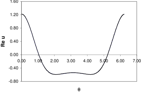
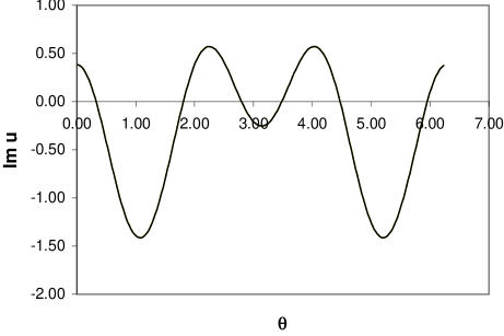
On the other hand, the situation is quite different if we allow the scatterer to be probed with waves of multiple frequencies.

Figures 3 and 4 show the real and imaginary parts for the same configurations $Q_{1}$ and $Q_{2}$ when the free space wave number $k_{0}$ is equal to $10.0$. Then $\Phi(Q_{2})=1.4307$. It is, of course, possible that there are configurations undistinguishable at this frequency, but, combining the output for several frequencies we can hope to achieve a reasonable recovery of the original scatterer. We show in the subsequent sections, that it is, indeed, the case. While there are many theoretical questions concerning the best, or a reasonable choice of frequencies, uniqueness for the IPM, stability estimates, etc., this work indicates the practicality of the multifrequency approach.

Figure 3: Real part of the solutions for configurations $Q_{1}$ (solid line) and $Q_{2}$ on the circle $S$ for $k_{0}=10$, $\Phi(Q_{2})=1.4307$.

Figure 4: Imaginary part of the solutions for configurations $Q_{1}$ (solid line) and $Q_{2}$ on the circle $S$ for $k_{0}=10$, $\Phi(Q_{2})=1.4307$.

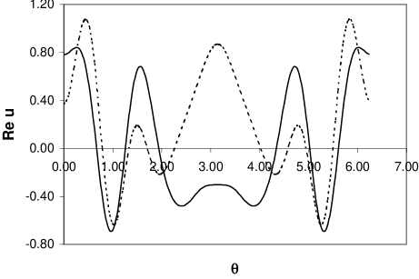
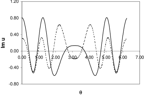
To illustrate this point further, let $P$ be the set of three free space wave numbers $k_{0}^{(p)}$ chosen to be

$$P=\{3.0,\ 6.5,\ 10.0\}\,.$$ (3.8)

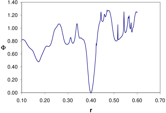
Figure 5 shows the profile of the functional $\Phi$ as a function of the variable $r\,,\,0.1\leq r\leq 0.6$ in the configurations $q_{r}$ with

$$n(x)=\begin{cases}0.49&0\leq|x|<r\\ 9.0&r\leq|x|<0.6\\ 1.0&0.6\leq|x|\leq 1.0\end{cases}$$

The best fit to data functional exhibits a sharp minimum at $r=.4$, thus there is a hope to identify the sought configuration.

Figure 5: Best fit profile for the configurations $q_{r}$; Multiple frequencies $P=\{3.0,\ 6.5,\ 10.0\}$.

4 Local Minimization Methods

Using the best fit to data functional $\Phi$ defined in (3.5), the IPM is reduced to a restrained minimization over the admissible set $A_{adm}$, defined in (3.6) and (3.7). It is well known that a multidimensional minimization is an extremely difficult problem, unless the objective function is ”well behaved”. The most important quality of such a cooperative function is the presence of just a few local minima. Unfortunately, this is, decidedly, not the case in many applied problems, and, in particular, for the problem under the consideration.

Figure 5 shows that our objective function $\Phi$ has many local minima even along this arbitrarily chosen one dimensional cross-section of the admissible set. There are sharp peaks and large gradients. Consequently, the gradient based methods (see [7], [11],[14],[17],[19],[22]) would not be successful for a significant portion of this region. It is also appropriate to notice that the dependency of $\Phi$ on its arguments is highly nonlinear. Thus, the gradient computations have to be done numerically, which makes them computationally expensive. More importantly, the gradient based minimization methods (as expected) perform poorly for these problems. These complications are avoided by considering conjugate gradient type algorithms which do not require the knowledge of the derivatives at all. One such method is the Powell’s method.

For an $N$-dimensional space the method can be described as follow (see [7]).

Powell’s Method

1. Initialize the set of directions $u_{i}$ to the basis vectors

   $$u_{i}=e_{i}\,,\quad i=1,2,\dots,N\,.$$

2. Save your starting position as $Q_{0}$.

3. For $i=1,\dots,N$ move $Q_{i-1}$ to the minimum along the direction $u_{i}$ and call this point $Q_{i}$.

4. For $i=1,\dots,N$, set $u_{i}=u_{i-1}$.

5. Set $u_{N}=P_{N}-P_{0}$.

6. Move $P_{N}$ to the minimum along direction $u_{N}$ and call this point $P_{0}$.

It can be shown that an iteration of this procedure produces a set $u_{i}$ of mutually conjugate directions, provided, as usual, that the objective function is quadratic. It also implies a quadratic convergence for nearly quadratic functions. The main difficulty here is that the obtained set of conjugate directions tends to become ”folded up”, that is linearly dependent. However, as noted in [7], the set of directions $u_{i}$ can be reset to the basis vectors $e_{i}$ after every $N$ or $N+1$ iterations of the basic procedure.

As explained in the next Section, we leave the global exploration of the admissible set to global minimization methods. A local minimization is used to explore an immediate vicinity of the initial configuration $Q\in\mbox{\Bb R}^{2M}$. With this goal in mind, given a configuration $Q\in\mbox{\Bb R}^{2M}$ and a direction $u$ in $\mbox{\Bb R}^{2M}$ we seek a minimum of $\Phi$ along this direction (by a bisection or a Golden Rule method) by restricting the probed points (at every minimization step) to the admissible set and by keeping them within a certain distance from the initial minimization point. This distance $d_{min}$ is determined a priori to be a percentage of the characteristic length of $A_{adm}$.

More precisely, the ”turtle” one-dimensional minimization is done as follows.

One-dimensional minimization

1. Let the starting position be $Q_{0}$.

2. Move from $Q_{0}$ along the given direction $u$ by the distance $d_{min}$ to obtain $Q_{1}\in A_{adm}$.

3. Find the minimum of $\Phi$ on the interval $[Q_{0},Q_{1}]$.

   If the minimum is attained inside the interval, then stop.

   If the minimum is attained at $Q_{0}$, then reverse the direction.

   If the minimum is attained at $Q_{1}$, then rename $Q_{0}=Q_{1}$, and repeat the procedure.

We have used Brent’s minimization Method [7] for the one-dimensional minimization in the step 3. This way the local minimum closest (the resolution is set up by $d_{min}$) to the starting configuration $Q_{0}$ is determined. The choise of $d_{min}$ has to be balanced between the desire to explore the fine structure of the objective function and the computational costs.

Now we can describe our Basic Local Minimization Method in $\mbox{\Bb R}^{2M}$. The above ”turtle” one-dimensional minimization procedure is used in all the minimization steps below.

Basic Local Minimization Method

1. Initialize the set of directions $u_{i}$ to the basis vectors

   $$u_{i}=e_{i}\,,\quad i=1,2,\dots,2M\,.$$

2. Save your starting position as $Q_{0}$.

3. For $i=1,\dots,2M$ move from $Q_{0}$ along the direction $u_{i}$ to find the point of minimum $Q_{i}^{t}$.

4. Reindex the directions $u_{i}$, so that (for the new indices) $\Phi(Q_{1}^{t})\leq\Phi(Q_{2}^{t})\leq,\dots,\Phi(Q_{2M}^{t})\leq\Phi(Q_{0})$.

5. For $i=1,\dots,2M$ move $Q_{i-1}$ to the minimum along the direction $u_{i}$ and call this point $Q_{i}$.

6. Set $v=Q_{2M}-Q_{0}$.

7. Move $Q_{2M}$ to the minimum along direction $v$ and call this point $Q_{0}$.

8. Repeat the above steps till a stopping criterion is satisfied.

Note, that we use the temporary points of minima $Q_{i}^{t}$ only to rearrange the initial directions $u_{i}$ in a different order. This method falls within the category of the Powell’s minimization methods, and, as mentioned above, produces conjugate directions and a quadratic convergence for nearly quadratic functions.

Still another refinement of the above algorithm has turned out to be necessary to produce a successful minimization. Since the dimension $2M$ of the minimization space was chosen a priori to be larger than $2N$, where $N$ is the (unknown) number of layers in the original scatterer, we expect that the sought point of minimum will be located in a lower dimensional subspace of the minimization space $\mbox{\Bb R}^{2M}$. This information available from the specific structure of our minimization problem appears to be nontrivial. Suffices to say, that all of our numerical experiments described in Section 6 have failed without the following (space dimension) ”reduction” procedure. The main idea behind it is to conduct the local minimization searches in as low-dimensional subspaces as possible. It is specific to the inverse scattering problem for multilayer scatterer.

If two adjacent layers have close refraction coefficients in the sense that the objective functional $\Phi$ is not changed much when the two layers assigned the same refraction coefficient, then these two layers can be replaced with just one occupying their place. The minimization problem becomes constrained to a lower dimensional subspace of $\mbox{\Bb R}^{2M}$ and the local minimization is done in this subspace. A similar procedure was used by us in [15] for the search of small subsurface objects.

Reduction Procedure

Let $\epsilon_{r}$ be a positive number.

1. Save your starting configuration $Q_{0}=(r_{1},r_{2},\dots,r_{M},n_{1},n_{2},\dots,n_{M})$ and $\Phi(Q_{0})$. Let the $M+1$-st layer be $D_{M+1}=\{r_{M}\leq|x|\leq R\}$ and $n_{M+1}=k_{0}^{2}$.

2. For $i=2,\dots,M+1$ replace $n_{i-1}$ in the layer $D_{i-1}$ by $n_{i}$. Compute $\Phi$ at the new configuration $Q_{i}^{d}$, and the difference $c_{i}^{d}=|\Phi(Q_{0})-\Phi(Q_{i}^{d})|$.

3. For $i=1,\dots,M$ replace $n_{i+1}$ in the layer $D_{i+1}$ by $n_{i}$. Compute $\Phi$ at the new configuration $Q_{i}^{u}$, and the difference $c_{i}^{u}=|\Phi(Q_{0})-\Phi(Q_{i}^{u})|$.

4. Find the smallest among the numbers $c_{i}^{d}$ and $c_{i}^{u}$. If this number is less than $\epsilon_{r}\Phi(Q_{0})$, then adjust the refraction coefficient to $n_{i}$ in the ”down” or ”up” layer accordingly. Replace the two adjacent layers with one occupying their place, and renumber the layers.

5. Repeat the above steps till no further reduction in the number of layers is occurring.

Note, that an application of the Reduction Procedure may or may not result in the actual reduction of layers.

Finally, the entire Local Minimization Method (LMM) consists of the following:

Local Minimization Method (LMM)

1. Let your starting configuration be $Q_{0}=(r_{1},r_{2},\dots,r_{M},n_{1},n_{2},\dots,n_{M})$.

2. Apply the Reduction Procedure to $Q_{0}$, and obtain a reduced configuration $Q_{0}^{r}$ containing $M^{r}$ layers.

3. Apply the Basic Minimization Method in $A_{adm}\bigcap\mbox{\Bb R}^{2M^{r}}$ with the starting point $Q_{0}^{r}$, and obtain a configuration $Q_{1}$.

4. Apply the Reduction Procedure to $Q_{1}$, and obtain a final reduced configuration $Q_{1}^{r}$.

5 Global Minimization Methods

Given an initial configuration $Q_{0}$ a local minimization method finds a local minimum near $Q_{0}$. On the other hand, global minimization methods explore the entire admissible set to find a global minimum of the objective function. While the local minimization is, usually, deterministic, the majority of the global methods are probabilistic in their nature. There is a great interest and activity in the development of efficient global minimization methods, see e.g. [4],[6]. Among them are the simulated annealing method ([20],[21]), various genetic algorithms [16], interval method, TRUST method ([2],[3]), etc. As we have already mentioned before, the best fit to data functional $\Phi$ has many narrow local minima. In this situation it is exceedingly unlikely to get the minima points by chance alone. Thus our special interest is for the minimization methods, which combine a global search with a local minimization. In [15] we developed such a method (the Hybrid Stochastic-Deterministic Method), and applied it for the identification of small subsurface particles, provided a set of surface measurements. The HSD method could be classified as a variation of a genetic algorithm with a local search with reduction. In this paper we consider the performance of two algorithms: Deep’s Method, and Rinnooy Kan and Timmer’s Multilevel Single-Linkage Method. Both combine a global and a local search to determine a global minimum. Recently these methods have been applied to a similar problem of the identification of particles from their light scattering characteristics in [29]. Unlike [29], our experience shows that Deep’s method has failed consistently for the type of problems we are considering. See [10] and [29] for more details on Deep’s Method.

Multilevel Single-Linkage Method (MSLM)

Rinnooy Kan and Timmer in [25] and [26] give a detailed description of this algorithm. Zakovic et. al. in [29] describe in detail an experience of its application to an inverse light scattering problem. They also discuss different stopping criteria for the MSLM. Thus, we only give here a shortened and an informal description of this method and of its algorithm.

In a pure Random Search method a batch $H$ of $L$ trial points is generated in $A_{adm}$ using a uniformly distributed random variable. Then a local search is started from each of these $L$ points. A local minimum with the smallest value of $\Phi$ is declared to be the global one.

A refinement of the Random Search is the Reduced Sample Random Search method. Here we use only a certain fixed fraction $\gamma<1$ of the original batch of $L$ points to proceed with the local searches. This reduced sample $H_{red}$ of $\gamma L$ points is chosen to contain the points with the smallest $\gamma L$ values of $\Phi$ among the original batch. The local searches are started from the points in this reduced sample.

Since the local searches dominate the computational costs, we would like to initiate them only when it is truly necessary. Given a critical distance $d$ we define a cluster to be a group of points located within the distance $d$ of each other. Intuitively, a local search started from the points within a cluster should result in the same local minimum, and, therefore, should be initiated only once in each cluster.

Having tried all the points in the reduced sample we have an information on the number of local searches performed and the number of local minima found. This information and the critical distance $d$ can be used to determine a statistical level of confidence, that all the local minima have been found. The algorithm is terminated (a stopping criterion is satisfied) if an a priori level of confidence is reached.

If, however, the stopping criterion is not satisfied, we perform another iteration of the MSLM by generating another batch of $L$ trial points. Then it is combined with the previously generated batches to obtain an enlarged batch $H^{j}$ of $jL$ points (at iteration $j$), which leads to a reduced sample $H^{j}_{red}$ of $\gamma jL$ points. The critical distance $d$ is reduced to $d_{j}$, (thus, the cluster’s size is redefined), a local minimization is attempted once within each cluster, the information on the number of local minimizations performed and the local minima found is used to determine if the algorithm should be terminated, etc.

The following is an adaptation of the MSLM method to the inverse scattering problem presented in Sections 2 and 3, with all the relevant notations. The LMM local minimization method introduced in the previous Section is used here to perform local searches.

MSLM

(at iteration $j$).

1. Generate another batch of $L$ trial points (configurations) from a random uniform distribution in $A_{adm}$. Combine it with the previously generated batches to obtain an enlarged batch $H^{j}$ of $jL$ points.

2. Reduce $H^{j}$ to the reduced sample $H^{j}_{red}$ of $\gamma jL$ points, by selecting the points with the smallest $\gamma jL$ values of $\Phi$ in $H^{j}$.

3. Calculate the critical distance $d_{j}$ by

   $$d_{j}^{r}=\pi^{-1/2}\left(\Gamma\left(1+\frac{M}{2}\right)R^{M}\frac{\sigma\ln jL}{jL}\right)^{1/M}\,,$$

   $$d_{j}^{m}=\pi^{-1/2}\left(\Gamma\left(1+\frac{M}{2}\right)(n_{high}-n_{low})^{M}\frac{\sigma\ln jL}{jL}\right)^{1/M}\,.$$

   $$d_{j}=\sqrt{(d_{j}^{r})^{2}+(d_{j}^{n})^{2}}$$

4. Order the sample points in $H^{j}_{red}$ so that $\Phi(Q_{i})\leq\Phi(Q_{i+1})\,,i=1,2,\dots,\gamma jL$. For each value of $i$, start the local minimization from $Q_{i}$, unless there exists an index $k<i$, such that $\|Q_{k}-Q_{i}\|\leq d_{j}$. Ascertain if the result is a known local minimum.

5. Let $K$ be the number of local minimizations performed, and $W$ be the number of different local minima found. Let

   $$W_{tot}=\frac{W(K-1)}{K-W-2}$$

   The algorithm is terminated if

   $$W_{tot}<W+0.5\,.$$ (5.1)

Here $\Gamma$ is the gamma function, and $\sigma$ is a fixed constant.

A related algorithm (the Mode Analysis) is based on a subdivision of the admissible set into smaller volumes associated with local minima. This algorithm is also discussed in [25] and [26]. From the numerical studies presented there, the authors deduce their preference for the MSLM.

6 Numerical Results

Introducing polar coordinates in (2.3) and separating the variables, equations for the total field $u(x)$ become

$$u_{1}(x)=\sum_{l=-\infty}^{\infty}a_{1,l}J_{l}(k_{1}|x|)e^{il\theta}$$

for $x\in D_{1}$,

$$u_{m}(x)=\sum_{l=-\infty}^{\infty}(a_{m,l}J_{l}(k_{m}|x|)+b_{m,l}Y_{l}(k_{m}|x|))e^{il\theta}$$

for $x\in D_{l},\,l=2,\dots,N$, and

$$u(x)=e^{ik<x,\nu>}+\sum_{l=-\infty}^{\infty}A_{l}H_{l}^{(1)}(k_{0}|x|)e^{il\theta}$$

for $x\in D:r_{N}\leq|x|\leq R$. Here $J_{l},Y_{l}$ are the Bessel functions of the first and second kind, $H_{l}^{(1)}$ is the Hankel function of the first kind, and $\nu$ is the direction vector of the incident wave. Since

$$e^{ik<x,\nu>}=\sum_{l=-\infty}^{\infty}i^{l}J_{l}(k_{0}|x|)e^{il\theta}$$

for $\nu=(1,0)$, the above equations and the conditions of continuity form a system of equations from which the field $u(x)$ can be calculated on the circle $S$. This solves the direct problem (2.2)-(2.3). Other methods of solution for such problems are known as well, see e.g. [18],[28]. Solving the direct problem for the set $P$ of three free wave numbers $k_{0}^{(p)}$ (see (3.8)), we obtain the total fields $u^{(p)}(x)$. Their restrictions to $S$ give the (simulated) data $g^{(p)}(\theta)$.

Our approach to the inverse problem IPM (see Section 2) is to recast it in the best fit to data form (3.5), and to minimize the objective functional $\Phi$ over $A_{adm}$. We have tested Deep’s global minimization method, the Multilevel Single-Linkage Method, and a Reduced Sample Random Search method. Each method was tried for three different original configurations $Q_{0}$ described below. The data $g^{(p)}(\theta)$ was computed at 120 angles $\theta_{l}=2\pi l/120,l=1,2,\dots,120$, and $\Phi$ was evaluated according to (3.4) and (3.5). This data was used with three different noise levels $\delta=0.00,0.03$ and $0.10$. More precisely, for the uniformly distributed on $[0,1]$ random variable $z$

$$g_{\delta}(\theta)=g(\theta)+\delta\|g\|(2z-1)(1+i)$$

for the noise level $\delta$.

Since our goal was to test the applicable algorithms, the values for the refraction coefficients, the size, the wave numbers, etc., were chosen arbitrarily at this time, that is without a regard for their possible physical relevancy. The original configurations are:

Configuration $Q_{0}^{(1)}$

This is a one layer cylinder $Q_{0}^{(1)}=(0.72,4.2025)$ with $N=1$ and $R=1.0$, see (3.2), that is the refraction coefficient is defined by

$$n(x)=\begin{cases}4.2025&0\leq|x|<0.72\\ 1.0&0.72\leq|x|\leq 1.0\end{cases}$$

Configuration $Q_{0}^{(2)}$

This is a two layer cylinder $Q_{0}^{(2)}=(0.4,0.6,0.49,9.0)$ with $N=2$ and $R=1.0$, that is

$$n(x)=\begin{cases}0.49&0\leq|x|<0.4\\ 9.0&0.4\leq|x|<0.6\\ 1.0&0.6\leq|x|\leq 1.0\end{cases}$$

Configuration $Q_{0}^{(3)}$

Three layer cylinder $Q_{0}^{(3)}=(0.3,0.7,0.8,4.0,25.0,9.0)$ with $N=3$ and $R=1.0$, that is

$$n(x)=\begin{cases}4.0&0\leq|x|<0.3\\ 25.0&0.3\leq|x|<0.7\\ 9.0&0.7\leq|x|<0.8\\ 1.0&0.8\leq|x|\leq 1.0\end{cases}$$

To identify these configurations we applied the global minimization methods of Section 5. In each one we let $M=4\,,R=1.0$. A priori bounds for the refraction coefficients were chosen to be $n_{low}=.04$ and $n_{high}=30.25$. Minor modifications to the description of the methods in Section 5 were introduced for the purpose of computational simplification. In particular, the minimization was done in $\sqrt{n_{m}}$ rather than in $n_{m}$ as stated there. This results in a rescaling of the admissible set. In each case, after a global minimum $Q_{min}$ was determined, the error of the identification

$$\epsilon_{err}=\frac{\int_{D}|n_{min}(x)-n(x)|}{\int_{D}n(x)}\,,$$ (6.1)

where $n(x)$ is the refraction coefficient of the original configuration $Q_{0}$, was computed to determine if the identification was successful. We distinguished between the two levels of a successful identification: $\epsilon_{err}<0.01$ and $\epsilon_{err}<0.1$.

Identification by Deep’s Method([10], [29])

Each test of the method consisted in 100 independent runs. Since $M=4$ the minimization was done in $\mbox{\Bb R}^{8}$. As we have already mentioned, the method failed every time. It seems, that the local minimization phase of Deep’s method (minimization over randomly selected parabolas) is not extensive enough to identify narrow local minima present in this problem. Also, the method does not use the Reduction Procedure (see Section 4), which, we think, is another reason for its failure. As in [29] we have also observed the cycling of the algorithm.

Identification by Reduced Sample Random Search Method

This method is presented in Section 5 in the subsection on the Multilevel Single- Linkage Method. The Local Minimization Method with the Reduction Procedure (as described in Section 4) was used in the local minimization phase. Chosen parameters $L=15000$ and $\gamma=0.01$ the performance of this method is the same as the Multilevel Single-Linkage Method. In fact, $L=15000$ is exactly the sample size in MSLM at it termination in our experiments. Since MSLM has the great advantage of a self-contained statistical stopping criteria (and from which the number 15000 was determined in the first place), it is, clearly, a preferred method.

Identification by Multilevel Single-Linkage Method

We have attempted to identify all 3 original configurations $Q_{0}^{(1)},Q_{0}^{(2)}$ and $Q_{0}^{(3)}$. Each one with no noise in the data ($\delta=0.00$) as well as with noise levels $\delta=0.03$ and $\delta=0.10$. Each of the 9 tests consisted of 10 independent runs. It took about 60 to 80 minutes on average to complete one run on a 333 MHZ PC. We used $M=4\,,R=1.0\,,\gamma=0.01$ and the sample size $L=200$. The parameter $\sigma$ was chosen to be equal to $1.0$. Value $\sigma=4.0$ was used in [26], and $\sigma=1.9$ in [12]. As in Deep’s Method above, a priori bounds for the refraction coefficients were chosen to be $n_{low}=.04$ and $n_{high}=30.25$. The value $\epsilon_{r}=0.1$ was used in the Reduction Procedure (see Section 4) during the local minimization phase.

As in other works on the clustering algorithm, we have found the stopping rule (5.1) to be unsatisfactory. In our experience the difference $W_{tot}-W$, while slightly decreasing with the number of performed minimizations, has quickly stabilized around the value of 5. Thus, the stopping criterion (5.1)

$$W_{tot}<W+0.5\,.$$

could not be attained. This issue has been discussed in [12] and [5], where a different stopping rule was suggested for functions with large number of local minima. Since the Bayesian stopping rule reflects the level of confidence in finding all the local minima, a relaxation of (5.1) would mean a smaller level of confidence, which still may be acceptable to assure that the global minimum is found among already performed local minimizations. We have chosen to replace (5.1) with

$$W_{tot}<W+0.5\quad\text{or}\quad W_{tot}<(1+\epsilon_{tot})W\,,$$ (6.2)

where $\epsilon_{tot}=0.03$.

As before

$$W_{tot}=\frac{W(K-1)}{K-W-2}\,,$$

where $K$ is the number of local minimizations performed, and $W$ is the number of different local minima found. Thus, the MSLM algorithm is terminated if (6.2) is satisfied. In our numerical experiments we have got the following average values $K=5000\,,W=150$, and $W_{tot}=155$.

Table 1: Identification by MSLM. Original configuration $Q_{0}^{(1)}$.

		Success rate1
Noise	Runs	$0.01$	$0.1$	Smallest $\Phi$
$\delta$=0.00	10	8	10	0.0000
$\delta$=0.03	10	9	10	0.0016
$\delta$=0.10	10	10	10	0.0178

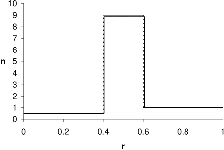
An example of a successful ($\epsilon_{err}<0.1$) identification for $Q_{0}^{(2)}$ and $\delta=0.10$ is shown on Figure 6. The identified configuration is a two layer cylinder

$$Q_{id}=(0.3966,0.5943,0.4684,9.203)\,,$$

with $\Phi(Q_{id})=0.0367,\epsilon_{err}=0.0480$. That is

$$n(x)=\begin{cases}0.4684&0\leq|x|<0.3966\\ 9.203&0.3966\leq|x|<0.5943\\ 1.0&0.5943\leq|x|\leq 1.0\end{cases}$$

Figure 6: Refraction coefficients $n(x)$ for the original $Q_{0}^{(2)}$ and the identified $Q_{id}$ (solid line) configurations. Data noise level $\delta=0.10$, $\Phi(Q_{id})=0.0367,\epsilon_{err}=0.0480$.

Table 2: Identification by MSLM. Original configuration $Q_{0}^{(2)}$.

		Success rate1
Noise	Runs	$0.01$	$0.1$	Smallest $\Phi$
$\delta$=0.00	10	10	10	0.0000
$\delta$=0.03	10	1	10	0.0034
$\delta$=0.10	10	2	9	0.0362

Table 3: Identification by MSLM. Original configuration $Q_{0}^{(3)}$.

		Success rate1
Noise	Runs	$0.01$	$0.2$	Smallest $\Phi$
$\delta$=0.00	10	2	7	0.0000
$\delta$=0.03	10	0	5	0.0071
$\delta$=0.10	10	0	5	0.0541

An example of a successful ($\epsilon_{err}<0.1$) identification for $Q_{0}^{(3)}$ and $\delta=0.03$ is a three layer cylinder

$$Q_{id}=(0.3030,0.7067,0.8079,4.071,24.528,8.857)\,,$$

with $\Phi(Q_{id})=0.00708,\epsilon_{err}=0.04125$. That is

$$n(x)=\begin{cases}4.071&0\leq|x|<0.3030\\ 24.528&0.3030\leq|x|<0.7067\\ 8.857&0.7067\leq|x|<0.8079\\ 1.0&0.8079\leq|x|\leq 1.0\end{cases}$$

7 Conclusions

The inverse scattering problem IPM is the identification of a multilayered scatterer by a set of observations on its boundary. Such problems have applications in science and engineering. In the case of the weak scattering approximation, many such problems can be solved by a linearized inversion. However, if the scattering is not weak, other methods of solution need to be developed. We have illustrated in Section 3, that an inversion based on just one frequency of the incident waves cannot be successful, since there are distinct configurations, producing practically the same observations. Introducing multiple frequencies, however, makes the inverse problem more amenable to a solution.

In this paper the inverse problem is transformed into the best fit to data minimization problem. This minimization is difficult, since the objective function is rugged and has many narrow local minima. A promising way to treat such a minimization is by a combination of global (probabilistic) and local (deterministic) minimization methods. In this paper we examined various local and global methods. Concerning the local minimization methods it was shown, that the Local Minimization Method (LMM) of Section 4 was successful, even where other considered methods failed. This method is a variation of a conjugate directions method with no use of partial derivatives. It has a quadratic convergence near quadratically shaped minima. However, even this method needs to be enhanced by a Reduction Procedure (Section 4). This procedure helps the minimization to take an advantage of the a priori available information, that the sought minima are likely to be found in certain lower dimensional subspaces of the entire minimization space.

For the global minimization part we considered Deep’s method and the Multilevel Single-Linkage Method. While Deep’s method failed, the MSLM was successful in many instances. It also has an important advantage of having termination criteria establishing a level of confidence, that the found minima contain the sought global minimum. Among the deficiencies of the MSLM are its slow execution, and inconsistency and failture to identify some configurations. There is still a problem in choosing an appropriate stopping rule. Thus, the MSLM provides a benchmark, against which the performance other methods can be judged and measured.

I would like to thank the referees for their valuable suggestions.

References

- [1] Athanasiadis C., Ramm A.G. and Stratis I.G. [1998] Inverse Acoustic Scattering by a Layered Obstacle, Inverse Problems, Tomography, and Image Processing. Ramm A. ed., Plenum Press, New York, 1-8.
- [2] Barhen J., Protopopescu V. [1996] Generalized TRUST algorithm for global optimization in State of the art in global optimization, (Floudas C., ed.), Kluwer, Dordrecht.
- [3] Barhen J., Protopopescu V., Reister D. [1997] TRUST: A deterministic algorithm for global optimization, Science, 276, May 16, 1094–1097.
- [4] Biegler L.T. (ed.) [1997] Large-scale optimization with applications. IMA volumes in mathematics and its applications. v.92-94, Springer-Verlag, New York.
- [5] Boender C.G.E. and Rinnooy Kan A.H.G. [1987] Bayesian stopping rules for multistart global optimization methods, Math. Program., 37, 59-80.
- [6] Bomze I.M. (ed.) [1997] Developments in Global Optimization, Kluwer Academia Publ., Dordrecht.
- [7] Brent P. [1973] Algorithms for minimization without derivatives, Prentice-Hall, Englewood Cliffs, NJ.
- [8] Colton D. and Kress R. [1992] Inverse Acoustic and Electromagnetic Scattering Theory, Springer-Verlag, Berlin.
- [9] Colton D. and Monk P. [1990] The Inverse Scattering Problem for acoustic waves in an Inhomogeneous Medium, Inverse problems in Partial Differential Equations. Colton D., Ewing R., Rundell W. eds., SIAM Publ. Philadelphia, 73-84.
- [10] Deep K. and Evans D.J. [1994] A parallel random search global optimization method, Technical Report 882, Computer Studies, Loughborough University of Technology.
- [11] Dennis J.E. and Schnabel R.B. [1983] Numerical methods for unconstrained optimization and nonlinear equations, Prentice-Hall, Englewood Cliffs, NJ.
- [12] Dixon L.C.W. and Jha M. [1993] Parallel algorithms for global optimization, J. Opt. Theor. Appl., 79, 385-395.
- [13] Ewing W.M, Jardetzky W.S and Press F. [1957] Elastic waves in Layered Media McGraw-Hill, New York.
- [14] Fletcher R. [1981] Practical methods of optimization v.2 John Wiley & Sons, New York.
- [15] Gutman S. and Ramm A.G. Application of the Hybrid Stochastic-deterministic Minimization Method to a Surface Data Inverse Scattering Problem, Fields Institute Communications, to appear.
- [16] Haupt R.L. and Haupt S.E. [1998] Practical genetic algorithms, John Wiley and Sons, Inc. New York.
- [17] Hestenes M. [1980] Conjugate direction methods in optimization, Applications of mathematics v.12 Springer-Verlag, New York.
- [18] Hu F.Q. [1995] A spectral boundary integral equation method for the 2D Helholtz equation J. Comp. Phys., 120, 340-347.
- [19] Jacobs D.A.H. (ed.) [1977] The state of the art in numerical analysis, Academic Press, London.
- [20] Kirkpatrick S., Gelatt C.D. and Vecchi M.P. [1983] Science, 220, 671–680.
- [21] Kirkpatrick S. [1984] Journal of Statistical Physics, 34, 975–986.
- [22] Polak E. [1971] Computational methods in optimization, Academic Press, New York.
- [23] Ramm A.G. [1986] Scattering by obstacles, D. Reidel, Dordrecht.
- [24] Ramm A.G. [1992] Multidimensional inverse scattering problems, Longman/Wiley, New York, Expanded Russian edition, MIR, Moscow, 1994.
- [25] Rinnooy Kan A.H.G. and Timmer G.T. [1987] Stochastic global optimization methods, part I: clustering methods, Mathematical Programming, 39, 27-56.
- [26] Rinnooy Kan A.H.G. and Timmer G.T. [1987] Stochastic global optimization methods, part II: multi level methods, Mathematical Programming, 39, 57-78.
- [27] Sabatier P.C. [1990] On the Scattering by Discontinuous Media. Inverse problems in Partial Differential Equations. Colton D., Ewing R., Rundell W. eds., SIAM Publ. Philadelphia, 85-100.
- [28] Schuster G.T. [1990] A fast exact numerical solution for the acoustic response of concentric cylinders with penetrable interfaces, J. Acoust. Soc. Am., 87, 495-502.
- [29] Zakovic S., Ulanowski Z. and Bartholomew-Biggs M.C. [1998] Application of global optimization to particle identification using light scattering, Inverse Problems, 14, 4, 1053–1067.