Mathematical Basis for Physical Inference

Albert Tarantola & Klaus Mosegaard Institut de Physique du Globe; 4, place Jussieu; F-75005 Paris; France; tarantola@ipgp.jussieu.frNiels Bohr Institute for Astronomy, Physics and Geophysics; Dept. of Geophysics; Haraldsgade 6; DK-2200 Copenhagen N; Denmark; klaus@osiris.gfy.ku.dk

Abstract

While the axiomatic introduction of a probability distribution over a space is common, its use for making predictions, using physical theories and prior knowledge, suffers from a lack of formalization. We propose to introduce, in the space of all probability distributions, two operations, the or and the and operation, that bring to the space the necessary structure for making inferences on possible values of physical parameters. While physical theories are often asumed to be analytical, we argue that consistent inference needs to replace analytical theories by probability distributions over the parameter space, and we propose a systematic way of obtaining such “theoretical correlations”, using the or operation on the results of physical experiments. Predicting the outcome of an experiment or solving “inverse problems” are then examples of the use of the and operation. This leads to a simple and complete mathematical basis for general physical inference.

1 Introduction

Why has mathematical physics become so universal? Does it allow the proper formulation of usual physical problems? Some reasons explain the popularity of mathematical physics. One reason is practical: mathematical physical theories may condensate a huge number of experimental results in a few functional relationships. Perhaps more importantly, these relationships usually have a tremendous power of extrapolation, allowing the prediction of the outcome of experiments never performed. Psychologically, this capacity of predicting the outcome of experiments gives the very satisfactory feeling of “understanding”.

Today, most scientists accept Popper’s (1) point of view that physics advances by postulating mathematical relations between physical parameters. While it is fully recognized that physical theories should be confronted with experiments, Popper emphasized that sucessful predictions, in whatever number, can never prove that a theory is correct, but one single observation that contradicts the predictions of the theory is enough to refute, to falsify the whole theory. He also stressed that these contradictory results are of uttermost importance for the advance of physics. When Michelson and Morley (2) could not find the predicted difference in the speed of light when the observer changes its velocity relative to the source, they broke the ground for the replacement of classical by relativistic mechanics.

Physical theories are conceptual models of reality. A good physical theory contains some or all of the following elements:

i) a modelisation of the space-time (for instance, as a four-dimensional continuum, or as a fractal entity)

ii) a modelisation of the objects of the “universe” (for instance, as point particles, or as continuous media)

iii) a recognition of the significant parameters in the experiments to be performed and a precise, operational, definition of these parameters

iv) mathematical relations postulated between these parameters, obtained by trying to obtain the best fit between observations and theoretical predictions.

While no physics is possible without points (i-iii) above, point (iv), i.e., postulating functional relations between the parameters to be used is not a necessity.

Any physical knowledge is uncertain, and estimation of uncertainties is crucial, for prosaic (e.g., preventing mechanical structures to collapse) as well as ethereal (e.g., using experimental results to decide between theories) reasons. The problem we face is that while considerable effort is spent in estimating experimental uncertainties, once a theory is postulated that is acceptable in view of these uncertainties, usual mathematical physics reasons as if the theory was exact. For instance, while we can use Gravitation Theory to predict the behaviour of space-time near the big-bang of certain models of the Universe, we have no means of estimating how uncertain are our predictions.

This is more striking when using analytical theories to solve the so-called “inverse problems” (3–6), where data, a priori information, and “physical theories” have to be used to make inferences about some parameters. The consideration of exact theories leads, at best, to inaccurate estimations, at worst, to mathematical inconsistencies (7).

This paper proposes an alternative to the common practice of postulating functional relationships between physical parameters. In fact, we propose a mathematical formalization of pure empiricism, as opposed to mathematical rationalism. Essentially, we suggest to replace functional relationships between physical parameters by well defined probability distributions over the parameter space.

The proposed formalism will, in some sense, only be a sort of “tabulation” of systematically performed experiments. In some aspects it will be less powerful than the one obtained through the use of analytical theories (it will not be able to extrapolate); in some aspects it will be more powerful (it will be able to properly handle actual uncertainties).

We will show how experiments could be, at least in principle, systematically performed so that a probability distribution in the parameter space is obtained that contains, as an analytical theory, the observed correlations between physical parameters, but, in addition, contains the full description of the attached uncertainties. We will also explain how, once such a theoretical probability distribution has been obtained, we can use it to make predictions —that will have attached uncertainties— or to use data to solve general inverse problems.

To fulfill this project we need to complete classical probability theory. Kolmogorov (8) proposed an axiomatic introduction of the notion of probability distribution over a space. The definition of conditional probability is then the starting point for doing inferences, as, for instance, through the use of the Bayes theorem. But the space of all probability distributions (over a given space) lacks structure. We argue below that there are two natural operations, the or and the and operation, to be defined over the probability distributions, that create the necessary structure: that of an inference space. We will see that while the or operation corresponds to an obvious generalization of “making histograms” from observed results, the and operation is just the right generalization of the notion of conditional probability.

2 The structure of an Inference Space

Before Kolmogorov (8), probability calculus was made using the intuitive notions of “chance” or “hazard”. Kolmogorov’s axioms clarified the underlying mathematical structure and brought probability calculus inside well defined mathematics. In this section we will recall these axioms. Our opinion is that the use in physical theories (where we have invariance requirements) of probability distributions, through the notions of conditional probability or the so-called Bayesian paradigm suffers today from the same defects as probability calculus suffered from before Kolmogorov. To remedy this, we introduce in this section, in the space of all probability distributions, two logical operations (or and and) that give the necessary mathematical structure to the space.

2.1 Kolmogorov’s concept of probability

A point ${\bf x}$ , that can materialize itself anywhere inside a domain ${\cal D}$ , may be realized, for instance, inside ${\cal A}$ , a subdomain of ${\cal D}$ . The probability of realization of the point is completely described if we have introduced a probability distribution (in Kolmogorov’s [8] sense) on ${\cal D}$ , i.e., if to every subdomain ${\cal A}$ of ${\cal D}$ we are able to associate a real number $P({\cal A})$ , called the probability of ${\cal A}$ , having the three properties:

$\bullet$ For any subdomain ${\cal A}$ of ${\cal D}$ , $P({\cal A})\geq 0$ .

$\bullet$ If ${\cal A}_{i}$ and ${\cal A}_{j}$ are two disjoint subsets of ${\cal D}$ , then, $P({\cal A}_{i}\cup{\cal A}_{j})=P({\cal A}_{i})+P({\cal A}_{j})$ .

$\bullet$ For a sequence of events ${\cal A}_{1}\supseteq{\cal A}_{2}\supseteq\cdots$ tending to the empty set, we have $P({\cal A}_{i})\rightarrow 0$ .

We will not necessarily assume that a probability distribution is normed to unity ( $P({\cal D})=1$ ). Although one refers to this as a measure, instead of a probability, we will not use this distinction. Sometimes, our probability distributions will not be normalizable at all ( $P({\cal D})=\infty$ ). We can only then compute the relative probabilities of subdomains.

These axioms apply to probability distributions over discrete or continuous spaces. Below, we will consider probability distributions over spaces of physical parameters, that are continuous spaces. Then, a probability distribution is represented by a probability density (note [9] explains the difference between a probability density and a volumetric probability).

In the next section, given a space ${\cal D}$ , we will consider different probability distributions $P\,,\,Q\dots$ Each probability distribution will represent a particular state of information over ${\cal D}$ . In what follows, we will use as synonymous the terms “probability distribution” and “state of information”.

2.2 Inference space

We will now give a structure to the space of all the probability distributions over a given space, by introducing two operations, the or and the and operation. This contrasts with the basic operations introduced in deductive logic, where the negation (“not”), nonexistent here, plays a central role. In what follows, the or and the and operation will be denoted, symbollically, by $\vee$ and $\wedge$ . They are assumed to satisfy the set of axioms here below.

The first axiom states that if an event ${\cal A}$ is possible for $(P$ or $Q)$ , then the event is either possible for $P$ or possible for $Q$ (which his is consistent with the usual logical sense for the “or”): For any subset ${\cal A}$ , and for any two probability distributions $P$ and $Q$ , the or operation satisfies

\left(P\vee Q\right)({\cal A})\neq 0\qquad\Longrightarrow\qquad P({\cal A})\neq 0\quad{\rm or}\quad Q({\cal A})\neq 0\ ,

the word “or” having here its ordinary logical sense.

The second axiom states that if an event ${\cal A}$ is possible for $(P$ and $Q)$ , then the event is possible for both $P$ and $Q$ (which is consistent with the usual logical sense for the “and”): For any subset ${\cal A}$ , and for any two probability distributions $P$ and $Q$ , the and operation satisfies

\left(P\wedge Q\right)({\cal A})\neq 0\qquad\Longrightarrow\qquad P({\cal A})\neq 0\quad{\rm and}\quad Q({\cal A})\neq 0\ ,

the word “and” having here its ordinary logical sense.

The third axiom ensures the existence of a neutral element, that will be interpreted below as the probability distribution carrying no information at all: There is a neutral element, $M$ for the and operation, i.e., it exists a $M$ such that for any probability distribution $P$ and for any subset ${\cal A}$ ,

\left(M\wedge P\right)({\cal A})=\left(P\wedge M\right)({\cal A})=P({\cal A})\ .

The fourth axiom imposes that the or and the and operations are commutative and associative, and, by analogy with the algebra of propositions of ordinary logic, have a distributivity property: the and operation is distributive with respect to the or operation.

The structure obtained when furnishing the space of all probability distributions (over a given space ${\cal D}$ ) with two operations or and and, satisfying the given axioms constitutes what we propose to call an inference space.

These axioms do not define uniquely the operations. Let $\mu({\bf x})$ be the particular probability density representing $M$ , the neutral element for the and operation, and let $p({\bf x}),q({\bf x})\dots$ be the probability densities representing the probability distributions $P,Q\dots$ Using the notations $(p\vee q)({\bf x})$ and $(p\wedge q)({\bf x})$ for the probability densities representing the probability distributions $P\vee Q$ and $P\wedge Q$ respectively, one realization of the axioms (the one we will retain) is given by

(p\vee q)({\bf x})=p({\bf x})+q({\bf x})\qquad;\qquad(p\wedge q)({\bf x})=\frac{p({\bf x})\,q({\bf x})}{\mu({\bf x})}\ ,

(1)

where one should remember that we do not impose to our probability distributions to be normalized.

The structure of an inference space, as defined, contains other useful solutions. For instance, the theory of fuzzy sets (10) uses positive functions $p({\bf x}),q({\bf x})\dots$ quite similar to probability densities, but having a different interpretation: the are normed by the condition that their maximum value equals one, and are interpreted as the “grades of membership” of a point ${\bf x}$ to the “fuzzy sets” $P,Q\dots$ . The operations or and and correspond then respectively to the union and intersection of fuzzy sets, and to the following realization of our axioms:

(p\vee q)({\bf x})={\rm max}\!\left(p({\bf x}),q({\bf x})\right)\qquad;\qquad(p\wedge q)({\bf x})={\rm min}\!\left(p({\bf x}),q({\bf x})\right)\ ,

(2)

where the neutral element for the and operation (intersection of fuzzy sets) is simply the function $\mu({\bf x})=1$ .

While fuzzy set theory is an alternative to classical probability (and is aimed at the solution of a different class of problems), our aim here is only to complete the classical probability theory. As explained below the solution given by equations 1 correspond to the natural generalisation of two fundamental operations in classical probability theory: that of “making histograms” and that of taking “conditional probabilities”. To simplify our language, we will sometimes use this correspondence between our theory and the fuzzy set theory, and will say that the or operation, when applied to two probability distributions, corresponds to the union of the two states of information, while the and operation corresponds to their intersection.

It is easy to write some extra conditions that distinguish the two solutions given by equations 1 and 2. For instance, as probability densities are normed using a multiplicative constant (this is not the case with the grades of membership in fuzzy set theory), it makes sense to impose the simplest possible algebra for the multiplication of probability densities $p({\bf x}),q({\bf x})\dots$ by constants $\lambda,\mu\dots$ :

\left[(\lambda+\mu)p\right]({\bf x})=\left(\lambda\,p\vee\mu p\right)({\bf x})\qquad;\qquad\left[\lambda(p\wedge q)\right]({\bf x})=\left(\lambda p\wedge q\right)({\bf x})=\left(p\wedge\lambda q\right)({\bf x})\ .

(3)

This is different from finding a (minimal) set of axioms characterizing (uniquely) the proposed solution, which is an open problem.

One important property of the two operations or and and just introduced is that of invariance with respect to a change of variables. As we consider probability distribution over a continuous space, and as our definitons are independent of any choice of coordinates over the space, it must happen that we obtain equivalent results in any coordinate system. Changing for instance from the coordinates ${\bf x}$ to some other coordinates ${\bf y}$ , will change a probability density $p({\bf x})$ to $\widetilde{p}({\bf y})=p({\bf x})\,|\partial{\bf x}/\partial{\bf y}|$ . It can easily be seen (11) that performing the or or the and operation, then changing variables, gives the same result than first changing variables, then, performing the or or the and operation.

Let us mention that the equivalent of equations 1 for discrete probability distributions is:

\left(p\vee q\right)_{i}=p_{i}+q_{i}\qquad;\qquad\left(p\wedge q\right)_{i}=\frac{p_{i}\,q_{i}}{\mu_{i}}\ .

(4)

Although the or and and notions just introduced are consistent with classical logic, they are here more general, as they can handle states of information that are more subtle than just the “possible” or “impossible” ones.

2.3 The interpretation of the or and the and operation

If an experimenter faces realizations of a random process and wants to investigate the probability distribution governing the process, he may start making histograms of the realizations. For instance, for realizations of a probability distribution over a continuous space, he will obtain histograms that, in some sense, will approach the probability density corresponding to the probability distribution.

A histogram is typically made by dividing the working space into cells, and by counting how many realizations fall inside each cell. A more subtle approach is possible. First, we have to understand that, in the physical sciences, when we say “a random point has materialized in an abstract space”, we may mean something like “this object, one among many that may exist, vibrates with some fixed period; let us measure as accurately as possible its period of oscillation”. Any physical measure of a real quantity will have attached uncertainties. As explained in section 3.2, this means that when, mathematically speaking, we measure “the coordinates of a point in an abstract space” we will not obtain a point, but a state of information over the space, i.e., a probability distribution.

If we have measured the coordinates of many points, the results of each measurement will be described by a probability density $p_{i}({\bf x})$ . The union of all these, i.e., the probability density

\left(p_{1}\vee p_{2}\vee\dots\right)({\bf x})=\sum_{i}p_{i}({\bf x})

(5)

is a finer estimation of the background probability density than an ordinary histogram, as actual measurement uncertainties are used, irrespectively of any division of the space into cells. If it happens that the measurement uncertainties can be described using box-car functions at fixed positions, then, the approach we propose reduces to the conventional making of histograms. This is illustrated in figure 1.

Refer to caption — Figure 1: Illustration of the or operation applied to probability distributions. A histogram is made (see top of the figure) by dividing the working space into cells, and by counting how many realizations fall inside each cell. A more subtle approach is possible. First, we have to understand that, in the physical sciences, when we say “a random point has materialized in an abstract space”, we may mean something like “this object, one among many that may exist, vibrates with some fixed period; let us measure as accurately as possible its period of oscillation”. Any physical measure of a real quantity will have attached uncertainties. This means that when, mathematically speaking, we measure “the coordinates of a point in an abstract space” we will not obtain a point, but a state of information over the space, i.e., a probability distribution. If we have measured the coordinates of many points, the results of each measurement will be described by a probability density $p_{i}(x)$ . The union of all these, i.e., the probability density $(p_{1}\vee p_{2}\vee\dots)({\bf x})=\sum_{i}p_{i}({\bf x})$ is a finer estimation of the background probability density than an ordinary histogram, as actual measurement uncertainties are used, irrespectively of any division of the space into cells. If it happens that the measurement uncertainties can be described using box-car functions (at fixed positions), then, the approach we propose reduces to the conventional making of histograms.

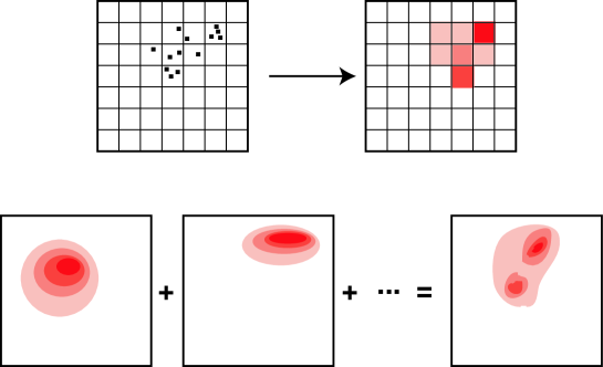
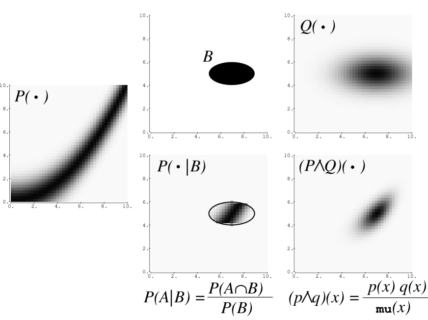
Figure 2 explains that our definition of the and operation is a generalization of the notion of conditional probability. A probability distribution $P(\ \cdot\ )$ is represented, in the figure, by its probability density. To any region ${\cal A}$ of the plane, it associates the probability $P({\cal A})$ . If a point has been realized following the probability distribution $P(\ \cdot\ )$ and we are given the information that, in fact, the point is “somewhere” inside the region ${\cal B}$ , then we can update the prior probability $P(\ \cdot\ )$ , replacing it by the conditional probability $P(\ \cdot\ |{\cal B})=P(\ \cdot\ \cap{\cal B})/P({\cal B})$ . It equals $P(\ \cdot\ )$ inside ${\cal B}$ and is zero outside (center of the figure). If instead of the hard constraint $x\in{\cal B}$ we have a soft information about the location of $x$ , represented by the probability distribution $Q(\ \cdot\ )$ (right of the figure), the intersection of the two states of information $P$ and $Q$ gives a new state of information (here, $\mu(x)$ is the probability density representing the state of null information, and, to simplify the figure, has been assumed to be constant). The comparison of the right with the center of the figure shows that the and operation generalizes the notion of conditional probability. In the special case where the probability density representing the second state of information, $Q(\ \cdot\ )$ , equals the null information probability density inside the domain ${\cal B}$ and is zero outside, then, the notion of intersection of states of information exactly reduces to the notion of conditional probability.

Now the interpretation of the neutral element for the and operation can be made clear. We postulated that the neutral probability distribution $M$ is such that for any probability distribution $P$ , $P\wedge M=P$ . This means that if a point is realized according to a probability distribution $P$ , and if a (finite accuracy) measure of the coordinates of the point produces the information represented by $M$ , the posterior probability distribution, $P\wedge M$ is still $P$ : the probability distribution $M$ is not carrying any information at all. Accordingly, we call $M$ the null information probability distribution. Sometimes, the probability density representing this state of null information is constant over all the space; sometimes, it is not, as explained in section 3.1. It is worth mentioning that this particular state of information enters in the Shannon’s definition of Information Content (12, 13).

It is unfortunate that, when dealing with probability distributions over continous spaces, conditional probabilities are often misused. Note (14) describes the so-called Borel-Kolmogorov paradox: using conditional probability densities in a space with coordinates $(x,y)$ will give results that will not be consistent with those obtained by the use of conditional probability densities on the same space but where other coordinates $(u,v)$ are used (if the change of coordinates is nonlinear). Jaynes (15) gives an excellent, explicit, account of the paradox. But his choice for resolving the paradox is different from our’s: while Jaynes just insists on the technical details of how some limits have to be taken in order to ensure consistency, we radically decide to abandon the notion of conditional probability, and replace it by the intersection of states of information (the and operation) which is naturally consistent under a change of variables, as demonstrated in note (11).

3 Physical parameters

Crudely speaking, a physical parameter is anything that can be measured. For a physical parameter, like a temperature, an electric field, or a mass, can only be defined by prescribing the experimental procedure that will measure it. Cook (16) discusses this point with lucidity.

The theory to be developed in this article will be illustrated by the analysis of objects that have a characteristic length, $L$ , affected by phenomena that have a characteristic period, $T$ . A measurement of a parameter is performed by realizing the conventional unit (i.e., the meter for a length, the second for a duration) and by comparing the parameter to the unit. We have then to turn to the definition of the units of time duration and of length.

At present, the second is defined as the duration of 9 192 631 770 periods of the radiation corresponding to the transition between the two hyperfine levels of the ground state of the cæsium-133 atom. Practically this means that a beam of cæsium-133 atoms are submitted to an electromagnetic field of adjustable frequency: when the imposed frequency is such that it causes the transition between the two hyperfine levels of the ground state of the atoms, the standard of frequency (and, thus, of period) has been realised.

Until 1991, the unit of length used to be defined independently of that of time duration. Now the meter is connected to the second by defining the value of the velocity of light as $c=$ 299 792 458 m s^-1. This means, in fact, that lengths are measured by measuring the time it takes light to traverse them (and then, converting to distance through this conventional value of $c$ ).

3.1 The noninformative probability density for physical parameters

Once a physical parameter has been defined, it is possible to associate to it a particular probability distribution, that will represent, when making a measurement, the absence of information on the possible outcome of the experiment.

Assume that, furnished with our definition of the unit of time duration, we wish to measure the period of some object. It can be the period of a rotating galaxy, or the period of a XVII-th century pendulum, or the period of a vibrating molecule: we do not know yet. Let us denote by $p(T)$ the probability density representing this state of total ignorance. The frequency $\nu$ associated to the period $T$ is $\nu=1/T$ . ¿From $p(T)$ we can, using the general rule of change of variables, deduce the probability density for the frequency: $q(\nu)=p(T)\,\left|dT/d\nu\right|=p(T)/\nu^{2}$ .

Now, the definition of the unit of time duration is undistinguishable from the definition of the unit of frequency. In fact, when trying to define the standard of time we said “when the imposed frequency is such that is causes the transition between the two hyperfine levels of the ground state of the atoms, the standard of frequency has been realised”, which shows how closely related are the reciprocal parameters period-frequency: we can not define the unit second without defining, at the same time, the unit Hertz.

We find here, at a very fundamental level, the class of reciprocal parameters analyzed by Harold Jeffreys (17). As he argued, the null information probability density must have the same form for the two parameters, i.e., $p(\cdot)$ and $q(\cdot)$ must be the same function. Then, the constraint $q(\nu)=p(T)/\nu^{2}$ , seen above, gives, up to a multiplicative constant, the solution

p(T)=\frac{1}{T}\qquad;\qquad q(\nu)=\frac{1}{\nu}\ .

(6)

The range of time durations (or of periods) considered in physics spans many orders of magnitude (from periods of atomic objects to cosmological periods). Physicists then often use a logarithmic scale, defining, for instance, $T^{\ast}=\log(T/T_{0})$ and $\nu^{\ast}=\log(\nu/\nu_{0})$ , where the two constants $\nu_{0}$ and $T_{0}$ can be arbitrary (18). Transforming the probability densities in 6 to the logarithmic variables gives $p^{\ast}(T^{\ast})=1$ and $q^{\ast}(\nu^{\ast})=1$ . The logarithmic variables (that take values on all the real line) have a constant probability density. This, is fact, is the deep interpretation of the $1/x$ probability densities in equations 6. The particular variables for which the probability density representing the state of null information is a constant over all the space can be named Cartesian: they are more “natural” than others, as are the usual Cartesian coordinates in Euclidean spaces (19). That these “Cartesian” variables are not only more natural, but also more practical than other variables, can be understood by considering that manufacturers of pianos space notes with constant increments not of frequency, but of the associated logarithmic variable.

We have seen that the definition of length is today related to that of time duration through the velocity of light. We could say that the electromagnetic wave of the radiation that defines the unit of time, defines, through its wavelength, the unit of distance. But, here again, we have a perfect symmetry between the wavelength and its inverse, the wavenumber. This is why we take the function $h(L)=1/L$ to describe the null information probability density for the length of an object (20).

3.2 Measuring physical parameters

To define the experimental procedure that will lead to a “measurement” we need to conceptualize the objects of the “universe”: do we have point particles or a continuous medium? Any instrument that we can build will have finite accuracy, as any manufacture is imperfect. Also, during the measurement act, the instrument will always be submitted to unwanted sollicitations (like uncontrolled vibrations).

This is why, even if the experimenter postulates the existence of a well defined, “true value”, of the measured parameter, she/he will never be able to measure it exactly. Careful modeling of experimental uncertainties is not easy, Sometimes, the result of a measurement of a parameter $p$ is presented as $p=p_{0}\pm\sigma$ , where the interpretation of $\sigma$ may be diverse. For instance, the experimenter may imagine a bell-shaped probability density around $p_{0}$ representing her/his state of information “on the true value of the parameter”. The constant $\sigma$ can be the standard deviation (or mean deviation, or other estimator of dispersion) of the probability density used to model the experimental uncertainty.

In part, the shape of this probability density may come from histograms of observed or expected fluctuations. In part, it will come from a subjective estimation of the defects of the unique pieces of the instrument. We postulate here that the result of any measurement can, in all generality, be described by defining a probability density over the measured parameter, representing the information brought by the experiment on the “true”, unknowable, value of the parameter. The official guidelines for expressing uncertainty in measurement, as given by the International Organization for Standardization (ISO) and the National Institute of Standards and Technology (21) although stressing the special notion of standard deviation, are consistent with the possible use of general probability distributions to express the result of a measurement, as advocated here.

Any shape of the density function is not acceptable. For instance, the use of a Gaussian density to represent the result of a measurement of a positive quantity (like an electric resistivity) would give a finite probability for negative values of the variable, which is inconsistent (a lognormal probability density, on the contrary, could be acceptable).

In the event of an “infinitely bad measurement” (like when, for instance, an unexpected event prevents, in fact, any meaningful measure) the result of the measurement should be described using the null information probability density introduced above. In fact, when the density function used to represent the result of a mesurement has a parameter $\sigma$ describing the “width” of the function, it is the limit of the density function for $\sigma\to\infty$ that should represent a measurement of infinitely bad quality. This is consistent, for instance, with the use of a lognormal probability density for a parameter like an electric resisitivity $r$ , as the limit of the lognormal for $\sigma\to\infty$ is the $1/r$ function, which is the right choice of noninformative probability density for $r$ .

Another example of possible probability density to represent the result of a measurement of a parameter $p$ is to take the noninformative probability density for $p_{1}<p<p_{2}$ and zero outside. This fixes strict bounds for possible values of the parameter, and tends to the noninformative probability density when the bounds tend to infinity.

The point of view proposed here will be consistent with the the use of “theoretical parameter correlations” as proposed in section 4.4, so that there is no difference, from our point of view, between a “simple measurement” and a measurement using physical theories, including, perhaps, sophisticated inverse methods.

4 Bayesian physical theories

Physical “laws” prevent us from setting arbitrarily some physical parameters. For instance, we can set the length of a tube where a free fall experiment will be performed, and we can also decide on the place and time of the experiment, but the time duration of the free fall is “imposed by Nature”. Physics in much about the analysis of these physical correlations between parameters.

Typically, a set ${\bf i}$ of independent parameters is identified, and experiments are performed in order to measure the values of a set ${\bf d}$ of dependent parameters (22). Analytical physical theories try then to express the result of the observations by a functional relationship ${\bf d}={\bf d}({\bf i})$ . In fact, saying that the independent parameters are “set” and the dependent parameters “measured” is an oversimplification, as all the parameters must be measured. And, as discussed in the previous section, uncertainties are present in every measurement. The values of the parameters that are set (the independent parameters) are never known exactly. The measures of the dependent parameters have always uncertainties attached. Assume we have made a large number of experiments, that show how the dependent parameters correlate with the independent ones. Within the error bars of the experimental results it will always be possible to fit an infinity of functional relationships of the form ${\bf d}={\bf d}({\bf i})$ . Adding more experimental points may help to discard some of the “theories”, but there will always remain an infinity of them.

We formalize this fact at a fundamental level, by replacing the need of a functional relationship by the use of a probability distribution in the space of all the parameters considered, representing the actual information we may have. Not only this point of view corresponds to a certain philosophy of physics, it also leads —as discussed below— to the only consistent formalism we know that is able to predict values of possible observations and of the attached uncertainties.

To be complete, we consider two cases where we may wish to analyze the physical correlations between parameters. The first case is when a repetitive phenomenon takes place spontaneously. The second case correspond to the case when an experimenter prompts a physical phenomenon, using an experimental arrangement.

4.1 The “contemplative” point of view

Consider an astronomer trying to analyze the “relationship” between the initial magnitude $m$ of shooting stars and the total distance $\Delta$ traveled by the meteors on the sky before disintegration. Each shooting star naturally appearing on the sky will allow one measurement of the two parameters $m$ and $\Delta$ to be performed (and possibly other significant parameters). As discussed above, each result of a measurement will be represented by a probability density. Let $\theta_{i}(m,\Delta)$ be the probability density representing the information obtained on the parameters $m$ and $\Delta$ of the $i$ -th shooting star.

When a large enough number of shooting starts has been observed, the correlation between the parameters $m$ and $\Delta$ is perfectly described by the probability density obtained by applying the or operation (as defined by the first of equations 1) to the probability distributions represented by $\theta_{1}(m,\Delta),\theta_{2}(m,\Delta),\dots$ , i.e., by the probability density $\theta(m,\Delta)=\sum_{i}\theta_{i}(m,\Delta)$ . If, more generally, the observed parameters are generically represented by ${\bf x}$ , and the result of the $i$ -th experiment, by the probability density $\theta_{i}({\bf x})$ , then,

\theta({\bf x})=\sum_{i}\theta_{i}({\bf x})\ .

(7)

The utility of this probability density will be explained in section 4.4.

4.2 The “experimental” point of view

Here, the independent parameters ${\bf i}$ are “set”, and the dependent parameters ${\bf d}$ measured. This case can be reduced to the previous case (the “contemplative” one) provided that the independent parameters $\bf i$ are “randomly generated” according to some reference probability distribution, as, for instance, the null information probability distribution discussed in section 3.1 (this guaranteeing, in particular, that any possible region of the space of independent parameters will eventually be sampled).

As above, if $\theta_{i}({\bf i},{\bf d})$ is the probability density representing the information on ${\bf i}$ and ${\bf d}$ obtained from the $i$ -th experiment, after a large enough number of experiments has been performed, the correlations between the dependent and the independent parameters are described by the probability density $\theta({\bf i},{\bf d})=\sum_{i}\theta_{i}({\bf i},{\bf d})$ . In general, if the whole set of parameters is generically represented by ${\bf x}=\{{\bf i},{\bf d}\}$ , and the result of the $i$ -th experiment, by the probability density $\theta_{i}({\bf x})$ , then equation 7 holds again.

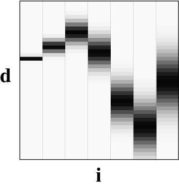
We have here assumed that the values of the independent parameters are set randomly according to their null information probability density. This directly leads to the “Bayesian theory” $\theta({\bf i},{\bf d})$ (this terminology being justified in section 4.4). A second option consists in defining physical correlations between parameters as a conditional probability density for the dependent parameters, given the independent parameters, $\theta({\bf d}|{\bf i})$ , but for the reasons explained elsewhere (14) the notion of conditional probability density, although a valid mathematical definition, is not of direct use for handling experimental results, unless enough care is taken. Assume, for instance, that the space of independent parameters is divided in boxes (multidimensional “intervals”) and that the independent parameters can be set to values that are certain to belong to one of the boxes. Performing the experiment for each of the possible “boxes” for the independent parameters, and, correspondingly, measuring the values of the dependent parameters ${\bf d}$ will produce states of information that are crudely represented in figure 3. This collection of states of information correspond to the conditional probability density $\theta({\bf d}|{\bf i})$ . The joint probability density in the $({\bf i},{\bf d})$ space that carries this information without carrying any information about the independent parameters (what we wish to call the “Bayesian theory”) is then the product of the conditional probability density $\theta({\bf d}|{\bf i})$ by the null information probability density for the independent paremeters, say $\mu_{\cal I}({\bf i})$ , i.e., the probability density

\theta({\bf i},{\bf d})=\theta({\bf d}|{\bf i})\,\mu_{\cal I}({\bf i})\ .

(8)

To be more accurate, if, in each experiment, the only thing we know about the independent parameters is the box where their value belongs, the measurement produces a probability density in the $({\bf i},{\bf d})$ space, say $\theta_{i}({\bf i},{\bf d})$ , that equals the product of a probability density over ${\bf d}$ (describing the result of the measurement of the dependent parameters) times a probability density that equals zero outside the box and equals the null information probability density inside the box. Applying the or operation to all these probability densitues will also give the result of equation 8.

Interpreting the conditional probability density $\theta({\bf d}|{\bf i})$ as simply putting some “error bars” around some “true functional relationship” ${\bf d}={\bf d}({\bf i})$ , that will always escape to our knowledge, or assuming that the experimental knowledge $\theta({\bf d}|{\bf i})$ represents is the “real thing”, and that there is no necessity of postulating the existence of a functional relationship, is a methaphysical question that will not change the manner of doing physical inference. As explained in section 4.4, inference will combine this “theoretical knowledge” represented by $\theta({\bf i},{\bf d})$ with further experiments using the and operation.

4.3 An example of Bayesian theory

The discussion on the noninformative priors, in section 3.1, was made without reference to a particular kind of object to be investigated. Let us now turn to analyze the physics of the fall of objects at the surface of the Earth.

Assume we have a tube (with vacuo inside) of length $L$ and we want to analyze the time $T$ it takes for a body to fall from the top to the bottom of the tube. Experiments readily show that

L-\frac{1}{2}\,g\,T^{2}\approx 0\ ,

(9)

where $g$ is the acceleration of gravity at the given location, but this “law” can not be exact for many reasons i) residual air resistance; ii) variation of gravity with height; iii) relativistic effects; iv) intrinsic (and so far unexplored) limitations of General Relativity; etc.

We want to replace the line $L=\frac{1}{2}\,g\,T^{2}$ by a probability density representing the actual knowledge that can be obtained from experiments. As explained in the previous section, the finite accuracy of any measurement will prevent the probability density from collapsing into a line “without thickness”.

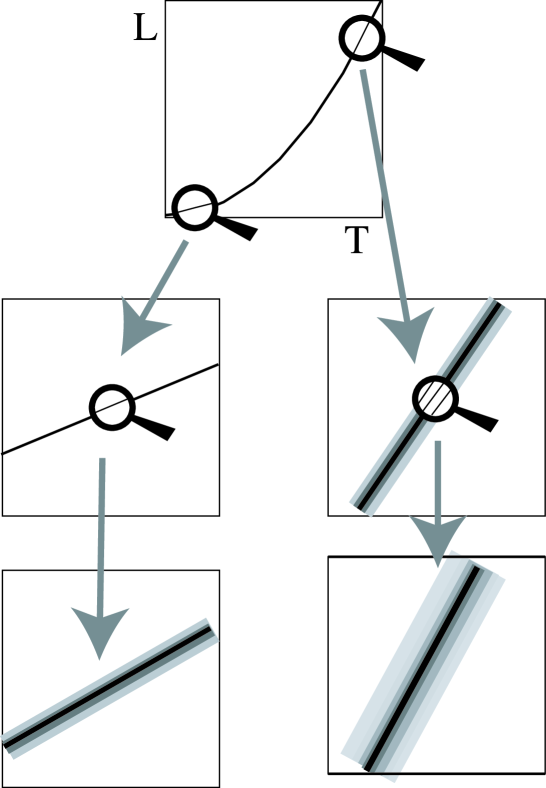
Let us face the actual problem of obtaining the probability density representing the theoretical/experimental knowledge on the physics of a falling body. In the case where the length $L$ is first set, and then the time $T$ of the fall of the body measured (this is, for instance, the way absolute gravimeters work, deducing, from the time $T$ , the local value of the acceleration of gravity $g$ ; we will later face the alternative possibility), the experimenter should receive tubes of different lengths $L_{1},L_{2}\dots$ randomly generated according to the null information probability density for the length of an object, i.e., with the probability density $1/L$ .

When the first tube is provided to him, the experimenter should perform the falling experiment and, using the best possible equipment, measure as accurately as possible the length $L$ of the tube given to him and the time $T$ it takes to the falling body to make the distance. This would provide him with a probability density $\theta_{1}(L,T)$ representing his knowledge of the realized value of the parameters. There is no reason for the uncertainties on $L$ and $T$ , as described by this probability density, to be independent. When a second tube, with random length, is provided to him, he should perform again the experiment and obtain a second probability density $\theta_{2}(L,T)$ . As already explained, the “Bayesian theory” corresponding to these experiments is then the union (in the sense defined above) of all the states of information obtained in all the individual experiments, when their number tends to infinity:

\theta(L,T)=\sum_{i=1}^{\infty}\theta_{i}(L,T)\,.

(10)

Figure 4 schematizes the sort of probability density such a method would produce (23).

We have explored the case where the length $L$ of the tube is first set and, then, the falling experiment is performed, measuring the time $T$ . The alternative is to fix the time duration $T$ first and, then, to perform the the falling experiment, measuring the length $L$ the falling body has traveled in that time. The two sorts of experiments are not identical, as the type of measurements performed will be different and will lead to different uncertainties. In this case, the experimenter is provided with time durations $T_{1},T_{2}\dots$ randomly selected according to the null information probability density for the period of a process, and obtains probability densities $\vartheta_{1}(L,T),\vartheta_{2}(L,T)\dots$ representing the results of the measurements. The union of all these states of information

\vartheta(L,T)=\sum_{i=1}^{\infty}\vartheta_{i}(L,T)\,,

(11)

would provide the “Bayesian theory” corresponding to that sort of experiment.

There is no reason for the two “Bayesian theories” thus obtained to be identical, as they correspond to a different type of experiment. We are then faced with the conclusion that the replacement of an analytical equation by a probability density will lead to probability densities attached to the precise experiment being performed. In fact, this is not so different to what would have been obtained when seeking for a functional relationship, as the “best fitting curve” for the first kind of experiments may not be the “best fitting” one for the second kind of experiments.

The formation of a “Bayesian theory” here made by summing small distributions (“histogramming”) can be understood in two ways. First, we could perfectly well proceed in this way in practice, performing systematic measurements of parameter correlations, using the best avalilable equipment. Alternatively, we can understand the proposed method as a thought experiment helping to clarify what “theoretical uncertainties” can be. These uncertainties can then be modeled using standard distributions (Gaussian, double exponential…) in such a way that usable but still realistic probability distributions in the parameter space can be defined and used as “Bayesian theories”, as in the example shown in note (23).

We will conclude this section with two remarks. First, it is not possible to sample a probability distribution that can not be normalized, as it is usually the case for the noninformative probabilities, like, for positive $x$ , the $1/x$ distribution. Then, practical lower and upper bounds have to be used. Second, the number of experimental “points” that have to be used in order to have a good practical approximation of a “Bayesian theory” depends on the accuracy of the measurements. Enough experiments have to be done so that the sum in equations 10 and 11 is smooth enough. The sharper the experimental design, the more experiments we will need (and the mode detail we will have).

4.4 Using a Bayesian physical theory

Assume that enough experiments have been made, by skilled people, using the best available equipment, following the guidelines of the previous section, so that the “Bayesian theory” $\theta(L,T)$ is available. Now a new tube is given to us, whose length has been randomly generated according to the null information probability density, $1/L$ . We perform the falling experiment, perhaps with a more modest equipment than that used to obtain the Bayesian theory, and measure the two parameters $L$ and $T$ , the result of the measurement being described by the state of information $\rho(L,T)$ . How can we combine this information with the Bayesian theory, so that we can ameliorate our knowledge on $L$ and $T$ ? We are exactly here in the situation where the notion of conditional probability (in fact, our generalization of it) applies: we know that we have a realization in the $(L,T)$ space generated according to the theoretical probability density $\theta(L,T)$ and we have a state of information on this particular realization that is described by the probability density $\rho(L,T)$ . The resulting state of information is then that obtained by applying the and operation to these two states of information (i.e., in the language defined above, by taking their intersection). This gives

\sigma(L,T)=\frac{\theta(L,T)\,\rho(L,T)}{\mu(L,T)}\quad.

(12)

In general, if ${\bf i}$ is the independent parameter set and ${\bf d}$ the dependent set,

\sigma({\bf i},{\bf d})=\frac{\theta({\bf i},{\bf d})\,\rho({\bf i},{\bf d})}{\mu({\bf i},{\bf d})}\,.

(13)

If the information content concerning $L$ contained in $\rho(L,T)$ is very high (the length of the tube is well known) while the information on $T$ is low, then, $\sigma(L,T)$ will essentially ameliorate our information on $T$ . This corresponds to the solution of a classical prediction problem in physics (how long it will take for a stone to fall from the top of the tower of Pisa?). Reciprocally, if the information content concerning $T$ contained in $\rho(L,T)$ is very high (the time of the fall is well known) while the information on the length of the tube is low, then, $\sigma(L,T)$ will essentially ameliorate our information on $L$ . Then, equation 12 corresponds to the solution of an “inverse problem”, where “data” is used to infer the values of the parameters describing some system. This use of the notion of intersection of states of information to solve inverse problems was advocated by Tarantola and Valette (5) and Tarantola (4), who showed that this method leads to results consistent with more particular techniques (like least squares of least absolute values) when some of the subtleties are ignored (theoretical uncertainties neglected, etc.).

We do not know of any alternative to our approach that solves consistently nonlinear inverse problems.

5 Discussion and Conclusion

Introducing Kolmogorov’s definition of probability distributions without introducing the two operations or and and, is like introducing the real numbers without introducing the sum and the product: we may compute, replacing clear mathematical objects by intuitive operations, but we are lacking an important structure of the space. The two operations we have introduced satisfy so obvious axioms that is difficult to imagine a simpler structure.

This structure may be used for many different inference problems, but we have chosen here an illustration in the realm of physics. We have replaced the notion of an analytical theory by the Bayesian notion of a probablity density representing all the experimentally obtained correlations between physical parameters, the space of independent parameters being visited randomly according to their null information probability density. Practically, some regions of the parameter space will not be accessible to investigation. Accordingly, the “result” of the measurement will be the null information probability density for the corresponding parameters. In other words, the “error bars” of a “Bayesian theory” may be large — or even infinite — for some regions of the parameter space. This is the typical domain where classical, analytical, theories extrapolate the equations that fit the observations made in a restricted region of the parameter space. No such extrapolation is allowed with our approach.

Although we have only shown a simple example (the Galilean experiment), the methodology has a large domain of application. As a further example, concerning tensor quantities, we could examine the dependence between stress and strain for a given medium. This would involve: i) mathematical definition of strain from displacement; ii) operational definition of stress; and iii) analysis of the stress-strain correlation using the method described in this article.

Analytical theories, when extrapolating, predict results that may not correspond to observations, when they are made. The theory is then “falsified” in the sense of Popper, and has to be corrected. A “Bayesian theory” can be indefinitely refined, as larger domains of the parameter space are accessible to experimentation, but never falsified. The present work shows that pure empiricism (as opposed to the mathematical rationalism of analytical theories) can be mathematically formalised. This formalism is the only one known by the authors that handles uncertainties consistently.

If physicists enjoy the game of extrapolation (as, for instance, when pushing Einstein’s gravity theory to the conditions prevailing in a Big Bang model of the Universe), engineers advance by performing experiments as close as possible to the conditions that will prevail “in the real thing”.

Using the approach here proposed, the “=” sign is only used for mathematical definitions, as, for instance, when defining a frequency from a period $\nu=1/T$ , or when using the mathematics associated to probability calculus. But the “=” sign is never used to describle physical correlations, that are, by nature, only approximate. These physical correlations are described by probability distributions. Some may see the systematic use of the “=” sign in mathematical physics as a misuse of mathematical concepts.

6 References and Notes

1

Popper, K.R., 1934, Logik der forschung, Viena; English translation: The logic of scientific discovery, Basic Books, New York, 1959.

2

Michelson, A.A. et E.W. Morley, 1887, Am. J. Sc. (3), 34, 333.

3

Backus, G., 1970a, Inference from inadequate and inaccurate data: I, Proc. Nat. Acad. Sci., 65, 1, 1–105; II, Proc. Nat. Acad. Sci., 65, 2, 281–287; III, Proc. Nat. Acad. Sci., 67, 1, 282–289.

4

Tarantola, A., 1987, Inverse problem theory; methods for data fitting and model parameter estimation, Elsevier; Tarantola, A., 1990, Probabilistic foundations of Inverse Theory, in: Geophysical Tomography, Desaubies, Y., Tarantola, A., and Zinn-Justin, J., (eds.), North Holland.

5

Tarantola, A., and Valette, B., 1982, Inverse Problems = Quest for Information, J. Geophys., 50, 159-170.

6

Mosegaard, K., and Tarantola, A., 1995, Monte Carlo sampling of solutions to inverse problems, J. Geophys. Res., Vol. 100, No. B7, 12,431–12,447.

7

An expression $d=d(m)$ connecting the data $d$ to the parameters $m$ is typically used with the notion of conditional probability density (through the Bayes theorem) to make inferences. As discussed in note (14), conditional probability densities do not have the necessary invariant properties when considering general (nonlinear) changes of variables.

8

Kolmogorov, A.N., 1933, Grundbegriffe der Wahrcheinlichkeitsrechnung, Springer, Berlin; Engl. trans.: Foundations of Probability, New York, 1950.

9

Usually, the probability $P({\cal A})$ of a domain ${\cal A}$ is calculated via an expression like $P({\cal A})=\int_{\cal A}dM({\bf x})\,p({\bf x})\ ,$ where $M({\cal A})$ is the volume (or measure) of ${\cal A}$ : $M({\cal A})=\int_{\cal A}dM({\bf x})\ .$ The existence of the volumetric probability $p({\bf x})$ is warranted by the Radon-Nicodym theorem if the probability $P$ is absolutely continous with respect to the measure $M$ (that is, if for any subdomain ${\cal A}$ , $M({\cal A})=0\Rightarrow P({\cal A})=0$ ). Alternatively, one may write $M({\cal A})=\int_{\cal A}{\underline{d}}{\bf x}\ {\overline{\mu}}({\bf x})$ and $P({\cal A})=\int_{\cal A}{\underline{d}}{\bf x}\ {\overline{p}}({\bf x})\ ,$ where the probability density ${\overline{p}}({\bf x})$ is defined by ${\overline{p}}({\bf x})={\overline{\mu}}({\bf x})\,p({\bf x})$ . The short notation ${\underline{d}}{\bf x}$ stands for $dx_{1}dx_{2}\dots$ . For instance, when considering a 3D Euclidean space with spherical coordinates, ${\underline{d}}{\bf x}=dr\,d\theta\,d\phi$ , ${\overline{\mu}}({\bf x})=r^{2}\,\sin\theta$ , and $dM({\bf x})={\overline{\mu}}({\bf x})\,{\underline{d}}{\bf x}=r^{2}\,\sin\theta\,dr\,d\theta\,d\phi$ . In a change of variables, a probability density ${\overline{p}}({\bf x})$ is multiplied by the Jacobian of the transformation, while the associated volumetric probability $p({\bf x})$ is invariant. The unfortunate gap existing between theoretical and practical presentations of probability theory induces frequent confusions between these two notions. The choice of the reference measure $M$ is obvious in geometrical spaces, as it is directly associated to the notion of volume. In more abstract spaces, like the spaces of physical parameters considered in this article, one has to introduce it explicitly. As explained elsewhere in the text, we interpret the probability density ${\overline{\mu}}({\bf x})$ as representing the “state of null information” on the considered parameters (interpretation consistent with the absolute continuity postulated by the Radon-Nicodym theorem). In the main text we always consider probability densities, not volumetric probabilities, and, to simplify notations, the overlines and underlines of this note are not written.

10

See, for instance, Kandel, A., 1986, Fuzzy mathematical techniques with applications, Addison-Wesley.

11

If $f$ represents a probability density function in some coordinate system, we will denote by $f^{\prime}$ the probability density in some transformed coordinates. Under such a transformation, a probability density gets its values multiplied by the Jacobian $J$ of the transformation: $f^{\prime}=J\,f$ . We have

f^{\prime}\vee g^{\prime}=(f\,J)+(g\,J)=(f+g)\,J=(p\vee q)^{\prime}\ ,

which demonstrates the invariance of the or operation under a change of variables. If $\mu$ represents the reference probability density (neutral element for the and operation), we also have

f^{\prime}\wedge g^{\prime}=\frac{(f\,J)\,(g\,J)}{\mu\,J}=\frac{f\,g}{\mu}\,J=(p\wedge q)^{\prime}\ ,

which demonstrates the invariance of the and operation under a change of variables.

12

Once one has agreed on the form of the probability density describing the state of null information, $\mu({\bf x})$ , Shannon’s (13) definition of information content of a probability density $p({\bf x})$ has to be written

I=\int_{\cal D}\!d{\bf x}\,p({\bf x})\,\log\frac{p({\bf x})}{\mu({\bf x})}\ .

Note that the “definition” $I=\int_{\cal D}\!d{\bf x}\,p({\bf x})\,\log p({\bf x})$ is not consistent, as it is not invariant under a change of variables.

13

Shannon, C.E., 1948, A mathematical theory of communication, Bell System Tech. J., 27, 379–423.

14

If ${\cal A}$ and ${\cal B}$ are two “events” (i.e., subsets of the space over which we consider a probability), with respective probability $P({\cal A})$ and $P({\cal B})$ , the conditional probability for the event ${\cal A}$ given the event $B$ is defined by $P({\cal A}|{\cal B})=P({\cal A}\cap{\cal B})/P({\cal B})$ . Consider, as an example, the Euclidean plane, with coordinates $(x,y)$ . A probability distribution over the plane can be represented by a probability density $p(x,y)$ . For finite $\Delta x$ and $\Delta y$ , one can consider the two events ${\cal A}=\left\{\matrix{x_{0}-\Delta x<x<x_{0}+\Delta x\cr-\infty<y<+\infty}\right\}$ and ${\cal B}=\left\{\matrix{-\infty<x<+\infty\cr y_{0}-\Delta y<y<y_{0}+\Delta y}\right\}$ representing respectively a “vertical” and an “horizontal” band of constant thicknesses $\Delta x$ and $\Delta y$ on the plane. In normal circumstances, the ratio $P({\cal A}\cap{\cal B})/P({\cal B})$ has a finite limit when $\Delta y\to 0$ . For variable $x$ , this defines a probability distribution over $x$ whose density is named the “conditional probability density over $x$ given $y=y_{0}$ ,” and that is given by

p(x|y=y_{0})=\frac{p(x,y_{0})}{\int_{-\infty}^{+\infty}\!dx\,p(x,y_{0})}\ .

It has to be realized that the probability density so defined depends on the fact that the limit is taken for a horizontal bar whose thickness tends to zero, this thickness being independent on $x$ . Should we, for instance, have assumed a band around $y=y_{0}$ with a thickness being a function of $x$ , we still could have defined a probability density, but it would not have been the same. The problem with this appears when changes of variables are considered. Changing for instance from the Cartesian coordinates $(x,y)$ to some other system of coordinates $(u,v)$ will change, according to the general rule, the (joint) probability density $p(x,y)$ to $q(u,v)=p(x,y)\left|\partial(x,y)/\partial(u,v)\right|$ . The line $y=y_{0}$ may become a line $v=v(u)$ , but any sensible interpretation of an expression like

q(u|v=v(u))=\frac{q(u,v(u))}{\int_{u_{\rm max}}^{u_{\rm min}}\!du\,q(u,v(u))}\ .

will consider a band of constant thickness $\Delta v$ around the line $v=v(u)$ . This band will not be (unless for linear changes of variable) the transformed of the band considered when using the variables $(x,y)$ . This implies that any computation made using conditional probability densities in a given system of cordinates will not correspond to the use of conditional probability densities in other systems of coordinates. Ignoring this fact leads to apparent paradoxes, as the so-called Borel-Kolmogorov paradox, described in detail by Jaynes(15). The approach we propose, where the notion of conditional probability is replaced by that of using the and operation on two probability distributions, is consistent with any change of variables, and will not lead, even inadvertently, to any paradoxical result.

15

Jaynes, E.T., 1995, Probability theory: the logic of science, Internet (ftp: bayes.wustl.edu).

16

Cook, A., 1994, The observational foundations of physics, Cambridge University Press.

17

Jeffreys, H., 1939, Theory of probability, Clarendon Press, Oxford.

18

For instance, they can be taken equal to the standards of time duration and of frequency, 9 192 631 770 Hz and (1/9 192 631 770) s respectively.

19

The noninformative probability density for the position of a point in an Euclidean space is easy to set in Cartesian coordinates: $p(x,y,z)=1/V$ , where $V$ is the volume of the region into consideration. Changing coordinates, one can obtain the form of the null information probability density in other coordinate systems. For instance, in spherical coordinates, $q(r,\theta,\varphi)=r^{2}\,\sin\theta/V$ .

20

There is an amusing consequence to the fact that it is the logarithm of the length (or the surface, or the volume) of an object that is the natural (i.e., Cartesian) variable. The Times Atlas of the World (comprehensive edition, Times books, London, 1983) starts by listing the surfaces of the states, territories, and principal islands of the world. The interesting fact is that the first digit of the list is far from having an uniform distribution in the range 1–9: the observed frequencies closely match the probability $p(n)=\log_{10}\left((n+1)/n\right)$ , (i.e., 30% of the occurrences are 1’s, 18% are 2’s,…, and less than 5% are 9’s), that is the theoretical distribution one should observe for a parameter whose probability density is of the form $1/x$ . A list using the logarithm of the surface should not present this effect, and all the digists 1–9 would have the same probability for appearing as first digit. This effect explains the amusing fact first reported by Frank Benford in 1939: that the books containing tables of logarithms (used, before the advent of digital computers, to make computations) have usually their first pages more damaged by use than their last pages…

21

Guide to the expression of uncertainty in measurement, International Organization of Standardization (ISO), Switzerland, 1993. B.N. Taylor and C.E. Kuyatt, 1994, Guidelines for evaluating and expressing the uncertainty of NIST measurement results, NIST technical note 1297.

22

In priciple, all the parameters of the Universe are linked, and we could say that the only possible thing to do is to observe their time evolution. Even the free will of the experimenter could be questioned. We rather take here the empirical point of view that some parameters of the Universe can be discarded, some independent parameters set (i.e., an experiment defined), and that we can observe the effects of the experiment.

23

As a matter of fact, we have simply represented the probability density

\theta(L,T)=\frac{k}{L\,T}\,\exp\left(-\frac{1}{2\,\sigma^{2}}\left(\log\frac{L}{\frac{1}{2}\,g\,T^{2}}\right)^{2}\right)

for the value $\sigma$ = 0.001 . Its marginal probability densities are $\theta_{L}(L)=\int_{T=0}^{T=\infty}dT\ \theta(L,T)=1/L$ and $\theta_{T}(T)=\int_{L=0}^{L=\infty}dL\ \theta(L,T)=1/T$ , this meaning that the probability density $\theta(L,T)$ carries no particular information on $L$ and on $T$ , but as this probability density takes significant values only when $L\approx\frac{1}{2}\,g\,T^{2}$ , it carries all the information on the physical correlation between $L$ and $T$ .

24

We thank Marc Yor for very helpful discussions concerning probability theory, and Dominique Bernardi for pointing to some important properties of real functions. Enrique Zamora helped to understand grille’s theory from an engineer point of view. B.N. Taylor and C.E. Kuyatt kindly sent us the very useful ISO’s “guide to the expression of uncertainty in measurement”. This work has been supported in part by the French Minister of National Education, the CNRS, and the Danish Natural Science Foundation.